note on the reheating temperature in starobinsky-type

General Relativity and Gravitation (2020) 52:116https://doi.org/10.1007/s10714-020-02770-3

RESEARCH ART ICLE

Note on the reheating temperature in Starobinsky-typepotentials

Jaume Haro1 · Llibert Aresté Saló2

Received: 23 July 2020 / Accepted: 18 November 2020 / Published online: 27 November 2020© The Author(s) 2020

AbstractThe relation between the reheating temperature, the number of e-folds and the spectralindex is shown for the Starobinsky model and some of its descendants through avery detailed calculation of these three quantities. The conclusion is that for viabletemperatures between 1 MeV and 109 GeV the corresponding values of the spectralindex enter perfectly in its 2σ C.L., which shows the viability of this kind of models.

Keywords Reheating · Number of e-folds · Starobinsky model

Contents

1 Introduction . . . . . . . . . . . . . . . . . . . . . . . . . . . . . . . . . . . . . . . . . . . . . 2

2 The number of e-folds . . . . . . . . . . . . . . . . . . . . . . . . . . . . . . . . . . . . . . . . 3

3 Different models . . . . . . . . . . . . . . . . . . . . . . . . . . . . . . . . . . . . . . . . . . . 4

3.1 Case n = 1: the exact Starobinsky model . . . . . . . . . . . . . . . . . . . . . . . . . . . . 7

3.2 Case n �= 1 . . . . . . . . . . . . . . . . . . . . . . . . . . . . . . . . . . . . . . . . . . . 8

4 The particular case wre = 1/3 . . . . . . . . . . . . . . . . . . . . . . . . . . . . . . . . . . . . 9

5 Conclusions . . . . . . . . . . . . . . . . . . . . . . . . . . . . . . . . . . . . . . . . . . . . . 12

References . . . . . . . . . . . . . . . . . . . . . . . . . . . . . . . . . . . . . . . . . . . . . . . . 12

B Llibert Aresté Saló[email protected]

Jaume [email protected]

1 Departament de Matemàtiques, Universitat Politècnica de Catalunya, Diagonal 647, 08028Barcelona, Spain

2 School of Mathematical Sciences, Queen Mary University of London, Mile End Road, London E14NS, UK

123

http://crossmark.crossref.org/dialog/?doi=10.1007/s10714-020-02770-3&domain=pdf

http://orcid.org/0000-0002-3812-8523

116 of 13 J. Haro, L. Aresté Saló

1 Introduction

The Starobinsky model based on R2-gravity in the Jordan frame [1], which was exten-sively studied in the literature (see for instance [2–5] and [6] for a detailed dynamicalanalysis), is one of the most promising scenarios to explain the inflationary paradigmproposed by A. Guth in [7] because it provides theoretical data about the power spec-trum of perturbations, which matches very well with the recent observational dataobtained by the Planck team [8]. In addition, contrary to the Guth’s paper, in [1] theauthor briefly details a successfully reheating mechanism based on the production ofparticles named scalarons whose decay products reheat the universe (see [3,9,10] fora detailed discussion of this mechanism), obtaining a reheating temperature around109 GeV [11] (see also [2] for the derivation of this reheating temperature when thedecay products are massless and minimally coupled with gravity).

Working in the Einstein frame, R2-gravity leads to the well-known Starobinskypotential [2], which has been recently studied as an inflationary potential, and thereheating temperature provided by the model is related to its corresponding spectralindex [12–14] (see also [15] for the calculation of the reheating temperature wheninflation come from a constant-roll era). However, contrary to [16,17] where theauthors consider the gravitational production of superheavy particles, in those papersthe reheating mechanism is not taken into account; instead of it, it is assumed that dur-ing the oscillations of the inflaton field the effective Equation of State (EoS) parameteris constant. From our viewpoint, it is difficult to understand how it is possible to makeany meaningful statements about reheating temperature without consideration of itsconcrete mechanisms, apart from the hypothesis of instant thermalization [18], whichhas to be still justified [19].

Anyway, although we do not discuss any reheating mechanism, the main goal ofthis note is to review these papers and find a very precise relation between the reheatingtemperature and the number of e-folds as a function of the spectral index of scalarperturbations, especially for the Starobinsky-type potentials that we have proposed byslightly modifying the Starobinsky potential so that its behavior near the origin is asa power law potential.

The work is organized as follows: in Sect. 2 we perform a very accurate calculationof the number of e-folds from the moment in which the pivot scale leaves the Hubblehorizon to the end of inflation, which will be used in Sect. 3 to relate the spectral indexprovided by the Starobinsky-type potentials with its reheating temperature. And weshownumerically that for temperatures between 1MeVand109 GeV the spectral indexranges in its 2σ Confidence Level, which means that these reheating temperatures arecompatiblewith themodel. Section4 is devoted to the studyof the particular casewherethe effective EoS parameter during the oscillations of the inflaton field is equal to 1/3.This is a very particular case where it is impossible to define exactly when the radiationstarts and, thus, that it is impossible to obtain the value of the reheating temperature.From what we show, we might argue that this case is physically unacceptable and allits consequences derived from it must be disregarded. However, one has to take intoaccount that a constant effective EoS during the oscillations of the inflaton is only anapproximation because the physics of this period is far from being clearly understood

123

Note on the reheating temperature in Starobinsky-type… of 13 116

and, thus, this approximation could lead to wrong conclusions. Finally, in the lastsection we discuss the obtained results.

The units used throughout the paper are � = c = 1 and the reduced Planck’s massis denoted by Mpl ≡ 1√

8πG∼= 2.44 × 1018 GeV.

2 The number of e-folds

First of all, we will assume that from the end of inflation to the beginning of theradiation era the effective Equation of State (EoS) parameter, namely wre followingthe notation of [13], is constant. However, from the end of inflation to the onset of theradiation era there is a transient period where the EoS is not constant. This period islargely unknown, as well as the mechanisms to produce and thermalize the relativisticplasma which reheats the universe. So, takingwre constant is an approximation whichin some cases could lead to incorrect results and interpretations.

In this situation, whenwre �= 1/3, the number of e-folds from the moment in whichthe pivot scale crosses the Hubble horizon to the end of inflation, namely Nk , is givenby (see formula (2.4) of [14])

Nk = ln(aeq/ak) + ln(ρeq/ρend)

3(1 + wre)+ 3wre − 1

12(wre + 1)ln(ρeq/ρre), (1)

where “eq” means the matter-radiation equality and “end” the end of the inflationaryperiod (see also [20,21]).

This expression could be written as

Nk = − ln(1 + zeq) + ln(Hk/kphys) + ln(ρeq/ρend)

3(1 + wre)

+ 3wre − 1

12(wre + 1)ln(ρeq/ρre), (2)

where z denotes the red-shift and kphy is the physical value of the pivot scale.We choose for example kphys ≡ k

a0= 0.05Mpc−1 ∼= 1.31 × 10−58Mpl , zeq =

3365, ρeq = π2

15 geqT4eq with geq = 3.36 and, from the adiabatic evolution of the

universe after reheating, we have that aeqTeq = a0T0 �⇒ Teq = (1 + zeq)T0, wherethe present CMB temperature is T0 = 2.725 K ∼= 2.35 × 10−4 eV.

We also consider ρre = ργ,re where ργ,re = π2

30 greT4re is the energy density of the

relativistic plasma (see for example the formula (3.51) of Mukhanov’s book [22]) atthe reheating time and gre = g(Tre) is the effective number of degrees of freedom atthe beginning of the radiation epoch. This is verified since after inflation the inflatonfield has completely decayed and, thus, ρφ plays no roll.

We use as well that ρend = 32Vend and, in order to get the value of Hk , we need

the spectrum of scalar perturbations when the pivot scale crosses the Hubble horizon

123


[23], namely

Pζ = H2k

8π2M2plεk

∼= 2 × 10−9, (3)

where

εk = M2pl

2

(Vφ(φk)

V (φk)

)2

, (4)

is the main slow-roll parameter at the crossing time.Then, we can write the number of e-folds as follows:

Nk = − ln(1 + zeq) + ln(Hk/kphys) + 1

4ln(ρeq/GeV

4)

+ ln(GeV4/ρend)

3(1 + wre)+ 3wre − 1

12(wre + 1)ln(GeV4/ρre)

∼= 96.5684 + 1

2ln εk + ln(GeV4/ρend)

3(1 + wre)

+ 3wre − 1

12(wre + 1)ln(GeV4/ρre), (5)

which only depends on the main slow roll parameter when the pivot scale leaves theHubble horizon, the effective EoS parameter wre, the energy density at the end ofinflation and the reheating temperature.

3 Different models

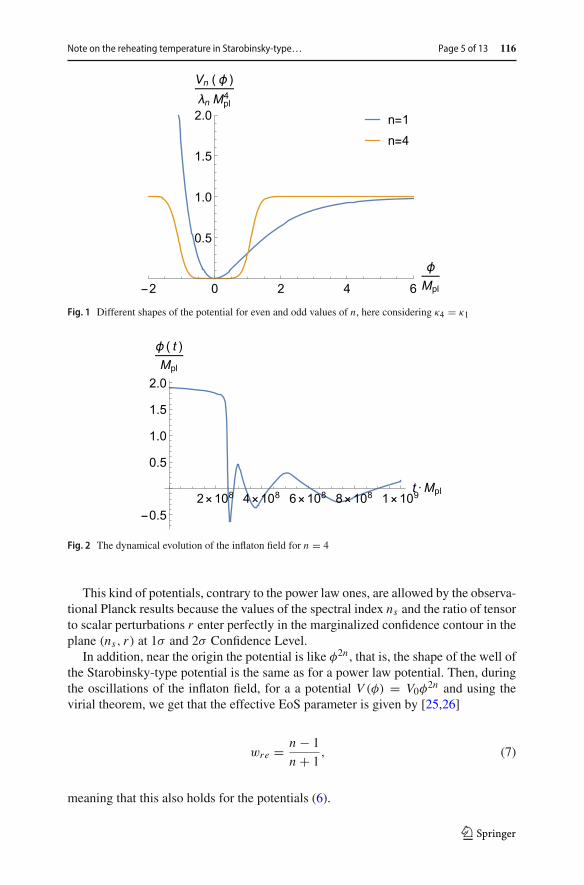
Wewill consider the following kind of Starobinsky-like potentials, depicted in Fig. 1,

Vn(φ) = λnM4pl(1 − e−κnφ

n/Mnpl )2, (6)

where λn and κn are dimensionless parameters (see also [24] for the study of otherpotentials slightly different from the Starobinsky one). As we have pointed out inthe introduction, these potentials represent a variation of the Starobinsky potential(the one when n = 1) with regards to the power of the scalar field. This n parameterenables us to mimic the behavior of a power law potential near the origin. Note that thefactor κ1 is required to be

√2/3 in the Starobinsky model in order to impose canonical

normalization of the scalar φ when passing from the R2 theory to the Einstein frame[2]. For n �= 1, given that this is not the case, we will be considering different possiblefactors so as to discuss for which ones the observations constraints are best fulfilled.

In Fig. 2 we see that for n even (the odd case is clear) the inflaton field oscillatesin the deep well potential after inflation, thus leaving its energy in order to produceenough particles to reheat the universe.

123


Fig. 1 Different shapes of the potential for even and odd values of n, here considering κ4 = κ1

Fig. 2 The dynamical evolution of the inflaton field for n = 4

This kind of potentials, contrary to the power law ones, are allowed by the observa-tional Planck results because the values of the spectral index ns and the ratio of tensorto scalar perturbations r enter perfectly in the marginalized confidence contour in theplane (ns, r) at 1σ and 2σ Confidence Level.

In addition, near the origin the potential is like φ2n , that is, the shape of the well ofthe Starobinsky-type potential is the same as for a power law potential. Then, duringthe oscillations of the inflaton field, for a a potential V (φ) = V0φ2n and using thevirial theorem, we get that the effective EoS parameter is given by [25,26]

wre = n − 1

n + 1, (7)

meaning that this also holds for the potentials (6).

123


On the other hand, dealing with the power spectrum of scalar perturbations, wehave that

εk = 2(κnn)2(

φk

Mpl

)2(n−1) e−2κnφnk /Mn

pl(1 − e−κnφ

nk /Mn

pl

)2

∼= 2(κnn)2(

φk

Mpl

)2(n−1)

e−2κnφnk /Mn

pl , (8)

and

ηk = M2plVφφ(φk)

V (φk)= 2κnn(n − 1)

(φk

Mpl

)n−2 e−κnφnk /Mn

pl

1 − e−κnφnk /Mn

pl(9)

−2(κnn)2(

φk

Mpl

)2(n−1)

e−κnφnk /Mn

pl1 − 2e−κnφ

nk /Mn

pl(1 − e−

√23φn

k /Mnpl

)2

∼= −2(κnn)2(

φk

Mpl

)2(n−1)

e−κnφnk /Mn

pl , (10)

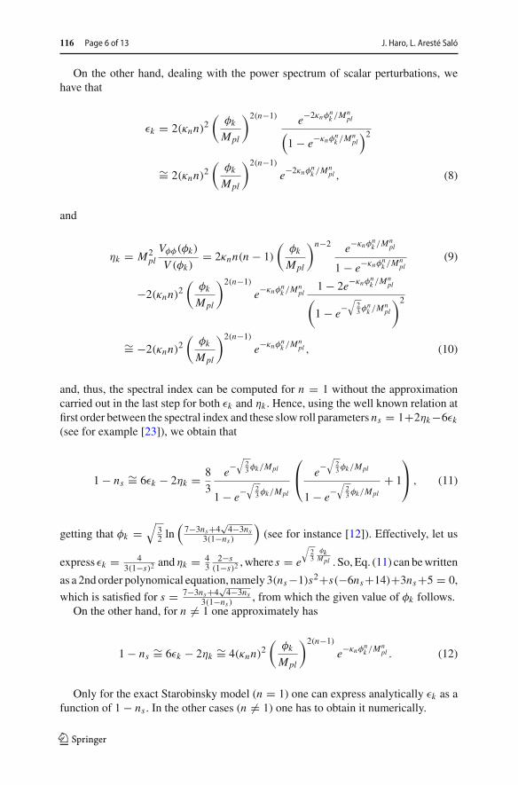
and, thus, the spectral index can be computed for n = 1 without the approximationcarried out in the last step for both εk and ηk . Hence, using the well known relation atfirst order between the spectral index and these slow roll parameters ns = 1+2ηk−6εk(see for example [23]), we obtain that

1 − ns ∼= 6εk − 2ηk = 8

3

e−√

23φk/Mpl

1 − e−√

23φk/Mpl

⎛⎝ e−

√23φk/Mpl

1 − e−√

23φk/Mpl

+ 1

⎞⎠ , (11)

getting that φk =√

32 ln

(7−3ns+4

√4−3ns

3(1−ns)

)(see for instance [12]). Effectively, let us

express εk = 43(1−s)2

andηk = 43

2−s(1−s)2

, where s = e

√23

φkMpl . So, Eq. (11) can bewritten

as a 2nd order polynomical equation, namely 3(ns−1)s2+s(−6ns+14)+3ns+5 = 0,

which is satisfied for s = 7−3ns+4√4−3ns

3(1−ns), from which the given value of φk follows.

On the other hand, for n �= 1 one approximately has

1 − ns ∼= 6εk − 2ηk ∼= 4(κnn)2(

φk

Mpl

)2(n−1)

e−κnφnk /Mn

pl . (12)

Only for the exact Starobinsky model (n = 1) one can express analytically εk as afunction of 1 − ns . In the other cases (n �= 1) one has to obtain it numerically.

123


Note also that inflation ends when

εend = 2(κnn)2(

φend

Mpl

)2(n−1) e−2κnφnend/Mn

pl(1 − e−κnφ

nend/Mn

pl

)2 = 1 (13)

and the value of φend can only be obtained analytically for the exact Starobinskymodel.

3.1 Case n = 1: the exact Starobinskymodel

Aswe have already explained in the introduction, this potential comes from R2-gravityin the Einstein frame (see for example [27] for a detailed explanation) and, since n = 1,wre = 0. In addition, from (13) one gets

φend = −√3

2ln(

√3(2 − √

3))Mpl ∼= 0.9402Mpl , (14)

obtaining

Vend = 4λ(2 − √3)2M4

pl �⇒ ρend = 6λ(2 − √3)2M4

pl , (15)

where we have used that at the end of inflation φ̇2end = V (φend) and, thus, ρend =

32V (ϕend).

To calculate the value of the parameter λ we use that H2k

∼= V (φk )

3M2pl

∼= λM2pl

3 . There-

fore, from the formula of the power spectrum of scalar perturbations (3) we obtain

λ ∼= 48π2 × 10−9εk, (16)

where εk = 43(1−s)2

, being s = 7−3ns+4√4−3ns

3(1−ns), as used in (11). With regards to the

number of e-folds, it is given by

Nk ∼= 96.5684 + 1

2ln εk + 1

3ln

(GeV3ρ

1/4re

ρend

), (17)

but can also be calculated using the formula

Nk =∫ tend

tkHdt = 1

Mpl

∫ φk

φend

1√2ε

dφ. (18)

So, using the values defined above, one gets that

Nk = 1

4

(3

(e

√23φk − e

√23φe

)− √

6(φk − φe)

), (19)

123


0.957 0.9585 0.96 0.96151

103

106

109

0.957 0.9585 0.96 0.9615

46

48

50

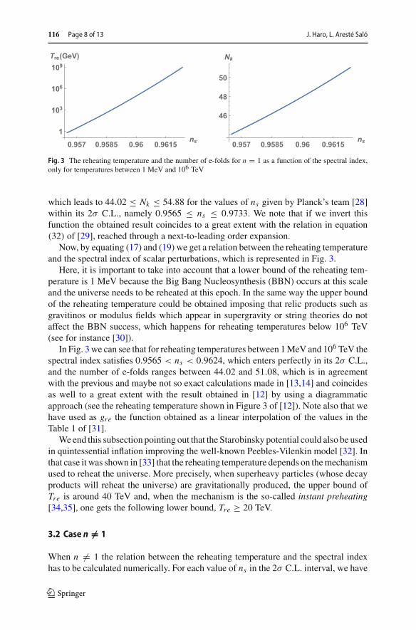
Fig. 3 The reheating temperature and the number of e-folds for n = 1 as a function of the spectral index,only for temperatures between 1 MeV and 106 TeV

which leads to 44.02 ≤ Nk ≤ 54.88 for the values of ns given by Planck’s team [28]within its 2σ C.L., namely 0.9565 ≤ ns ≤ 0.9733. We note that if we invert thisfunction the obtained result coincides to a great extent with the relation in equation(32) of [29], reached through a next-to-leading order expansion.

Now, by equating (17) and (19) we get a relation between the reheating temperatureand the spectral index of scalar perturbations, which is represented in Fig. 3.

Here, it is important to take into account that a lower bound of the reheating tem-perature is 1 MeV because the Big Bang Nucleosynthesis (BBN) occurs at this scaleand the universe needs to be reheated at this epoch. In the same way the upper boundof the reheating temperature could be obtained imposing that relic products such asgravitinos or modulus fields which appear in supergravity or string theories do notaffect the BBN success, which happens for reheating temperatures below 106 TeV(see for instance [30]).

In Fig. 3we can see that for reheating temperatures between 1MeV and 106 TeV thespectral index satisfies 0.9565 < ns < 0.9624, which enters perfectly in its 2σ C.L.,and the number of e-folds ranges between 44.02 and 51.08, which is in agreementwith the previous and maybe not so exact calculations made in [13,14] and coincidesas well to a great extent with the result obtained in [12] by using a diagrammaticapproach (see the reheating temperature shown in Figure 3 of [12]). Note also that wehave used as gre the function obtained as a linear interpolation of the values in theTable 1 of [31].

We end this subsection pointing out that the Starobinsky potential could also be usedin quintessential inflation improving the well-known Peebles-Vilenkin model [32]. Inthat case it was shown in [33] that the reheating temperature depends on themechanismused to reheat the universe. More precisely, when superheavy particles (whose decayproducts will reheat the universe) are gravitationally produced, the upper bound ofTre is around 40 TeV and, when the mechanism is the so-called instant preheating[34,35], one gets the following lower bound, Tre ≥ 20 TeV.

3.2 Case n �= 1

When n �= 1 the relation between the reheating temperature and the spectral indexhas to be calculated numerically. For each value of ns in the 2σ C.L. interval, we have

123


numerically solved Eqs. (11) and (13) in order to find the values of φk and φend . Thenwe have used the value of εk in Eq. (8) in order to calculate the number of e-folds Nk

as stated in (16). And finally we have obtained the reheating temperature by settingthis value equal to the one in Eq. (5). As in the case n = 1 we have taken as gre thelinear interpolations of the values in the table 1 of [31].

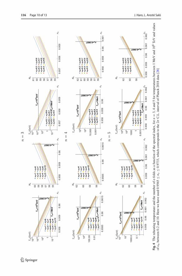
In Fig. 4, taking viable reheating temperatures from 1 MeV to 106 TeV, we havedepicted the corresponding values of the spectral index for several models and severalvalues of κn , showing that they enter in its 2σ C.L. We have also represented thecorresponding number of e-folds for these values of ns . Themodels studied correspondto the values n = 3, 4 and 5 which are respectively equal to the following values ofthe effective EoS parameter, wre = 1/2, 3/5 and 2/3. Note that in all these casesthe reheating temperature decreases as ns grows, in opposite to what happens whenn = 1. This arises from the fact that the last term in Eq. (5) vanishes for n = 2. As aconsequence, Tre is constant in ns for n = 2, thus increasing (resp. decreasing) as afunction of ns for n < 2 (resp. n > 2).

For each of these values of n we have studied the results for values of κn between0.2 and 10 and we have also drawn straight lines for the bounds for the reheatingtemperature aswell as the lower limit of the allowed interval for ns at 1σ C.L. accordingto the results of [28], given that all the depicted values of ns are already in the 2σ C.L.interval. While for all the values of n and κn that we have represented the allowedvalues of the reheating temperatures fall within the 2σ C.L. interval of ns , when both nand κn become higher a wider range of the allowed reheating temperatures correspondto a value of ns within the 1σ C.L. interval. With regards to the number of efolds, allthe obtained values (namely between 55 and 65) are feasible. And, as far as the ratio ofthe tensor to scalar perturbations is concerned, it does not influence our results sincein all the cases it is verified that r < 10−5.

Therefore, we see that by modifying the power law behavior at the origin of theStarobinsky potential, we obtain values of the reheating temperature and the numberof e-folds from the crossing of the Hubble horizon of the pivot scale until the endof inflation which continue being in accordance with the allowed ones by taking thespectral index within the 2σ CL of the Planck 2018 data [28]. So, we have found anew group of potentials which match as well as the Starobinsky potential with theobservational data and, moreover, they contain a parameter n which can be tunned inorder to adjust the behavior that we want to have near the origin.

4 The particular casewre = 1/3

This situation is obtained for our potentials when n = 2 and it has been already shownthat it is impossible to obtain neither the value of the reheating temperature Tre, northe number of e-folds from the end of inflation to the beginning of the radiation eraNre = ln( are

aend). The reason is that, in order to obtain the values of Tre and Nre, one

needs to know the beginning of the radiation epoch, i.e., when the energy density of thelight particles obtained from the decay of the inflaton field starts to dominate, whichdoes not happen in this case because during the oscillations of inflaton the effectiveEoS parameter is the same as in the radiation era [12–14].

123


Fig.4

The

reheatingtemperature

andthenu

mberof

e-foldsas

afunctio

nof

thespectralindex,

forn

=3,

4and5fortemperaturesbetw

een1MeV

and10

6TeVandvalues

ofκnbetween0.2and10

.Herewehave

used

0.95

65≤

n s≤

0.97

33,w

hich

correspo

ndsto

the2σ

C.L.intervalo

fPlanck

2018

data[28]

123


However, in this particular case it is possible to calculate the effective number ofdegrees of freedom at the beginning of reheating, which is obtained using the formula(2.12) of [13]:

gre =(43

11

)4 (π2

30

)3(

Hka0T0

eNkρ1/4endk

)12

. (20)

Now, taking into account that Hk/k = 1/ak and that akeNk = aend , one gets

gre =(43

11

)4 (π2

30

)3(

a0T0

aendρ1/4end

)12

(21)

and, using that from the end of inflation to the matter-radiation equality the effectiveEoS parameter is 1/3, which implies aendρ

1/4end = aeqρ

1/4eq , one finally obtains

gre =(43

11

)4 (π2

30

)3(

(1 + zeq)T0

ρ1/4eq

)12

. (22)

This formula is very interesting because it depends neither on the shape of thepotential during inflation, nor on the pivot scale. Instead it only depends on the numberof degrees of freedom at the matter-radiation equality. Effectively, using once againthat Teq = (1 + zeq)T0 and ρeq = π2

15 geqT4eq , with geq = 3.36 the number of degrees

of freedom at the matter-radiation equality, we get the following abnormally smallnumber

gre = 43

11

(43

22geq

)3 ∼= 0.6256, (23)

which is in contradiction with the values of the effective degrees of freedom (see forinstance Figure 1 of [31]). In fact its minimum value is approximately geq = 3.36,which is obtained at the matter-radiation equality.

Therefore, one might conclude that the case wre = 1/3 has to be disregarded,as well as all its consequences. For example, the assumption that the value of gre isapproximately 100 (see for instance the Section 2.1 of [13]) and also the consequencesderived in Section 5 of [12]. However, as we have already explained at the end of theIntroduction and at the beginning of Sect. 2, one has to be cautious with this kind ofresult because a constant effective EoS is only an approximation. Hence, in order tobe sure of their viability, one must deal with a more realistic model containing a welldefined reheating mechanism telling us which is the real evolution of the effectiveEoS parameter from the end of inflation to the beginning of the radiation era (see forexample [36] where the authors study some viable models obtaining numerically theevolution of the effective EoS parameter during this period) .

123


5 Conclusions

In this short note we have proved that for Starobinsky-type potentials of the formλnM4

pl(1−e−κnφn/Mn

pl )2 depending on twodimensionless parametersλn and κn (whichseem to be the best for predicting the values of the power spectrum of perturbationsaccording to the recent observations) the reheating temperature ranges in awide regionof its allowed values, which span below 106 TeV—in order that the production of relicssuch as gravitinos or modulus fields in supergravity theories do not affect the successof the BBN—and above 1 MeV to ensure that the reheating was previous to the BBN.In fact, as one can see from Fig. 4, the higher the values of n and κn are, a widerrange of allowed reheating temperatures enters in the 1σ C.L. of the spectral index,indicating that in this sense the model is more favored. In addition, for the special casen = 1 (the Starobinsky model) our results are in agreement with the ones obtainedindependently in [12] by following a different scheme named diagrammatic approach.

Finally, we have also studied the particular case when the effective EoS parameterduring the oscillations of the inflaton field is equal to 1/3 showing that this case leadsto an absurd value of the number of degrees of freedom at the reheating time, meaningthat this ideal situation (in a more realistic model the effective EoS is not constant)and its consequences must be disregarded.

Acknowledgements We would like to thank Professor Starobinsky for carefully reading our manuscriptand also for his comments and suggestions that have been very helpful for improving our work, to GabrielGermán for useful conversations, and also to the referee for its criticism which has been very important toimprove our work. This investigation has been supported by MINECO (Spain) Grant MTM2017-84214-C2-1-P and in part by the Catalan Government 2017-SGR-247.

OpenAccess This article is licensedunder aCreativeCommonsAttribution 4.0 InternationalLicense,whichpermits use, sharing, adaptation, distribution and reproduction in any medium or format, as long as you giveappropriate credit to the original author(s) and the source, provide a link to the Creative Commons licence,and indicate if changes were made. The images or other third party material in this article are includedin the article’s Creative Commons licence, unless indicated otherwise in a credit line to the material. Ifmaterial is not included in the article’s Creative Commons licence and your intended use is not permittedby statutory regulation or exceeds the permitted use, you will need to obtain permission directly from thecopyright holder. To view a copy of this licence, visit http://creativecommons.org/licenses/by/4.0/.

References

1. Starobinsky, A.A.: A new type of isotropic cosmological models without singularity. Phys. Lett. B 91,99 (1980)

2. De Felice, A., Tsujikawa, S.: f(R) theories. Living Rev. Rel. 13, 3 (2010). arXiv:1002.4928 [gr-qc]3. Vilenkin, A.: Classical and quantum cosmology of the Starobinsky inflationary model. Phys. Rev. D

32, 2511 (1985)4. Nojiri, S., Odintsov, S.D., Oikonomou, V.K.: Gravity theories on a nutshell: inflation, bounce and

late-time evolution. Phys. Rep. 692, 1–104 (2017). arXiv:1705.11098 [gr-qc]5. Nojiri, S., Odintsov, S.D.: Unified cosmic history in modified gravity: from F(R) theory to Lorentz

non-invariant models. Phys. Rep. 505, 59–144 (2011). arXiv:1011.0544 [gr-qc]6. Amorós, J., de Haro, J., Odintsov, S.D.: On R + αR2 loop quantum cosmology. Phys. Rev. D 89,

104010 (2014). arXiv:1402.3071 [gr-qc]7. Guth, A.: The inflationary universe: a possible solution to the horizon and flatness problems. Phys.

Rev. D 23, 347 (1981)

123

http://creativecommons.org/licenses/by/4.0/

http://arxiv.org/abs/1002.4928





8. Ade, P.A.R., et al.: Planck 2015 results. XX. Constraints on inflation. Astron. Astrophys. 594, A20(2016). arXiv:1502.02114 [astro-ph.CO]

9. Starobinsky, A.A.: Proc. of the Second Seminar Quantum Theory of Gravity (Moscow, 13–15 Oct1981), pp. 58–72. INR Press, Moscow (1982). (reprinted in: Quantum Gravity, eds. M. A. Markov, P.C. West, Plenum Publ. Co., New York, (1984), pp. 103–128)

10. Haro, J.: Gravitational particle production: a mathematical treatment. J. Phys A Math. Theor. 44,205401 (2011)

11. Gorbunov, D.S., Panin, A.G.: Scalaron the mighty: producing dark matter and baryon asymmetry atreheating. Phys. Lett. B 700, 157–162 (2011). arXiv:1009.2448 [hep-ph]

12. German, G.: Precise determination of the inflationary epoch and constraints for reheating (2020).arXiv:2002.11091 [astro-ph.CO]

13. Cook, J.L., Dimastrogiovanni, E., Easson, D.A., Krauss, L.M.: Reheating predictions in single fieldinflation. arXiv:1502.04673 [astro-ph.CO]

14. Rehagen, T., Gelmini, G.B.: Low reheating temperatures in monomial and binomial inflationary poten-tials. JCAP 06, 039 (2015). arXiv:1504.03768 [hep-ph]

15. Oikonomou, V.K.: Reheating in constant-roll F(R) gravity. Mod. Phys. Lett. A 32, 1750172 (2017).arXiv:1706.00507 [gr-qc]

16. Hashiba, S., Yokoyama, J.: Gravitational reheating through conformally coupled superheavy scalarparticles. JCAP 01, 028 (2019). arXiv:1809.05410 [gr-qc]

17. Chung, D.J.H., Kolb, E.W., Long, A.J.: Gravitational production of super-Hubble-mass particles: ananalytic approach. JHEP 01, 189 (2019). arXiv:1812.00211 [hep-ph]

18. McDonough, E.: The cosmological heavy ion collider: fast thermalization after cosmic inflation (2020).arXiv:2001.03633 [hep-th]

19. Starobinsky, A.A.: Private communication (2020)20. Dai, L., Kamionkowski, M., Wang, J.: Reheating constraints to inflationary models. Phys. Rev. Lett.

113, 041302 (2014). arXiv:1404.6704 [astro-ph.CO]21. Muñoz, J.B., Kamionkowski, M.: Equation-of-state parameter for reheating. Phys. Rev. D 91, 043521

(2015). arXiv:1412.0656 [astro-ph.CO]22. Mukhanov, V.: Physical Foundations of Cosmology. Cambridge University Press, Cambridge (2005)23. Bassett, B.A., Tsujikawa, S., Wands, D.: Inflation dynamics and reheating. Rev. Mod. Phys. 78, 537

(2006). arXiv:astro-ph/050763224. Sebastiani, L., Cognola, G., Myrzakulov, R., Odintsov, S.D., Zerbini, S.: Nearly Starobinsky inflation

from modified gravity. Phys. Rev. D 89, 023518 (2014). arXiv:1311.0744 [gr-qc]25. Turner, M.S.: Coherent scalar-field oscillations in an expanding universe. Phys. Rev. D 28, 1243 (1983)26. Ford, L.H.: Gravitational particle creation and inflation. Phys. Rev. D 35, 2955 (1987)27. Kehagias, A., Dizgah, A.M., Riotto, A.: Comments on the Starobinsky model of inflation and its

descendants. Phys. Rev. D 89, 043527 (2014). arXiv:1312.1155 [hep-th]28. Akrami, Y., et al.: Planck 2018 results. X. Constraints on inflation (2018). arXiv:1807.06211 [astro-

ph.CO]29. Roest, D.: Universality classes of inflation. JCAP 01, 007 (2014). arXiv:1309.1285 [hep-th]30. Giudice, G.F., Kolb, E.W., Riotto, A.: Largest temperature of the radiation era and its cosmological

implications. Phys. Rev. D 64, 023508 (2001). arXiv:hep-ph/000512331. Husdal, L.: On effective degrees of freedom in the early universe. Galaxies 4(4), 78 (2016).

arXiv:1609.04979 [astro-ph.CO]32. Peebles, P.J.E., Vilenkin, A.: Quintessential inflation. Phys. Rev. D 59, 063505 (1999).

arXiv:astro-ph/981050933. Haro , J., Aresté Saló, L.: The spectrum of gravitational waves, their overproduction in quintessential

inflation and its influence in the reheating temperature (2020). arXiv:2004.11843 [gr-qc]34. Felder, G., Kofman, L., Linde, A.: Instant preheating. Phys. Rev. D 59, 123523 (1999).

arXiv:hep-ph/981228935. Felder, G., Kofman, L., Linde, A.: Inflation and preheating in NO models. Phys. Rev. D 60, 103505

(1999). arXiv:hep-ph/990335036. Lozanov, K.D., Amin, M.A.: Self-resonance after inflation: oscillons, transients and radiation domi-

nation. Phys. Rev. D 97, 023533 (2018). arXiv:1710.06851 [astro-ph.CO]

Publisher’s Note Springer Nature remains neutral with regard to jurisdictional claims in published mapsand institutional affiliations.

123












http://arxiv.org/abs/astro-ph/0507632





http://arxiv.org/abs/hep-ph/0005123


http://arxiv.org/abs/astro-ph/9810509





note on the reheating temperature in starobinsky-type

Documents