note 12 of 5e statistics with economics and business applications chapter 8 test of hypotheses for...
Post on 22-Dec-2015
218 views
TRANSCRIPT

Note 12 of 5E
Statistics with Economics and Statistics with Economics and Business ApplicationsBusiness Applications
Chapter 8 Test of Hypotheses for Means and Proportions
Null and alternative hypotheses, test statistic, type I and II errors, significance level, p-value

Note 12 of 5E
ReviewReview
I. I. What’s in last lecture?What’s in last lecture?Small-Sample Estimation of a Population Mean Chapter 7
II. II. What's in the next two lectures?What's in the next two lectures?Hypotheses tests for means and proportions Read Chapter 8

Note 12 of 5E
IntroductionIntroduction• Setting up and testing hypotheses is an essential part of
statistical inference. In order to formulate such a test, usually some theory has been put forward, either because it is believed to be true or because it is to be used as a basis for argument, but has not been proved.
• Hypothesis testing refers to the process of using statistical analysis to determine if the differences between observed and hypothesized values are due to random chance or to true differences in the samples.– Statistical tests separate significant effects from
mere luck or random chance. – All hypothesis tests have unavoidable, but
quantifiable, risks of making the wrong conclusion.

Note 12 of 5E
IntroductionIntroduction
• Suppose that a pharmaceutical company is concerned that the mean potency of an antibiotic meet the minimum government potency standards. They need to decide between two possibilities:– The mean potency does not exceed the required minimum potency.– The mean potency exceeds the required minimum potency.
• This is an example of a test of hypothesistest of hypothesis..

Note 12 of 5E
IntroductionIntroduction
• Similar to a courtroom trial. In trying a person for a crime, the jury needs to decide between one of two possibilities:– The person is guilty.– The person is innocent.
• To begin with, the person is assumed innocent.• The prosecutor presents evidence, trying to
convince the jury to reject the original assumption of innocence, and conclude that the person is guilty.

Note 12 of 5E
Five Steps of a Statistical TestFive Steps of a Statistical Test A statistical test of hypothesis consist of five stepsA statistical test of hypothesis consist of five steps
1.1. Specify statistical hypothesis which include a Specify statistical hypothesis which include a null null hypothesishypothesis HH00 and a and a alternative hypothesisalternative hypothesis HHaa
2.2. Identify and calculate Identify and calculate test statistictest statistic
3.3. Identify distributionIdentify distribution and find and find p-valuep-value
4. Make a decision to reject or not to reject the null hypothesis
5. State conclusion

Note 12 of 5E
Null and Alternative HypothesisNull and Alternative Hypothesis
The null hypothesis, HThe null hypothesis, H00::– The hypothesis we wish to falsify – Assumed to be true until we can prove
otherwise.
The alternative hypothesis, HThe alternative hypothesis, Haa:: – The hypothesis we wish to prove to be true
Court trial: Pharmaceuticals:
H0: innocent H0: does not exceeds required potency
Ha: guilty Ha: exceeds required potency
Court trial: Pharmaceuticals:
H0: innocent H0: does not exceeds required potency
Ha: guilty Ha: exceeds required potency

Note 12 of 5E
Examples of HypothesesExamples of Hypotheses
You would like to determine if the diameters of the ball bearings you produce have a mean of 6.5 cm.
H0: =6.5
Ha: 6.5
(Two-sided or two tailed alternative)

Note 12 of 5E
Do the “16 ounce” cans of peaches meet the claim on the label (on the average)?
Notice, the real concern would be selling the consumer less than 16 ounces of peaches.
H0:
Ha: < 16
One-sided or one-tailed alternative
Examples of HypothesesExamples of Hypotheses

Note 12 of 5E
Comments on Setting up HypothesisComments on Setting up Hypothesis
• The null hypothesis must contain the equal sign.
This is absolutely necessary because the distribution of test statistic requires the null hypothesis to be assumed to be true and the value attached to the equal sign is then the value assumed to be true.
• The alternate hypothesis should be what you are really attempting to show to be true.
This is not always possible.
There are two possible decisions: reject or fail to reject the null hypothesis. Note we say “fail to reject” or “not to reject” rather than “accept” the null hypothesis.

Note 12 of 5E
Two Types of ErrorsTwo Types of ErrorsThere are two types of errors which can occur in a statistical test:• Type I error: reject the null hypothesis when it is true• Type II error: fail to reject the null hypothesis when it is false
Actual Fact
Jury’s Decision
Guilty Innocent
Guilty Correct Error
Innocent Error Correct
Actual Fact
Your
Decision
H0 true H0 false
Fail to reject H0
Correct Type II Error
Reject H0 Type I Error Correct

Note 12 of 5E
Error AnalogyError AnalogyConsider a medical test where the hypotheses are equivalent to
H0: the patient has a specific disease
Ha: the patient doesn’t have the diseaseThen,
Type I error is equivalent to a false negative(I.e., Saying the patient does not have the disease
when in fact, he does.)Type II error is equivalent to a false positive(I.e., Saying the patient has the disease when, in
fact, he does not.)

Note 12 of 5E
Two Types of ErrorsTwo Types of Errors
We want to keep the both α and β as small as possible. The value of is controlled by the experimenter and is called the significance level.
Generally, with everything else held constant, decreasing one type of error causes the other to increase.
Define:
= P(Type I error) = P(reject H0 when H0 is true)
P(Type II error) = P(fail to reject H0 when H0 is false)

Note 12 of 5E
Balance Between Balance Between and and • The only way to decrease both types of error
simultaneously is to increase the sample size.
• No matter what decision is reached, there is always the risk of one of these errors.
• Balance: identify the largest significance level as the maximum tolerable risk you want to have of making a type I error. Employ a test procedure that makes type II error as small as possible while maintaining type I error smaller than the given significance level .
Note 12 of 5E
Test StatisticTest Statistic
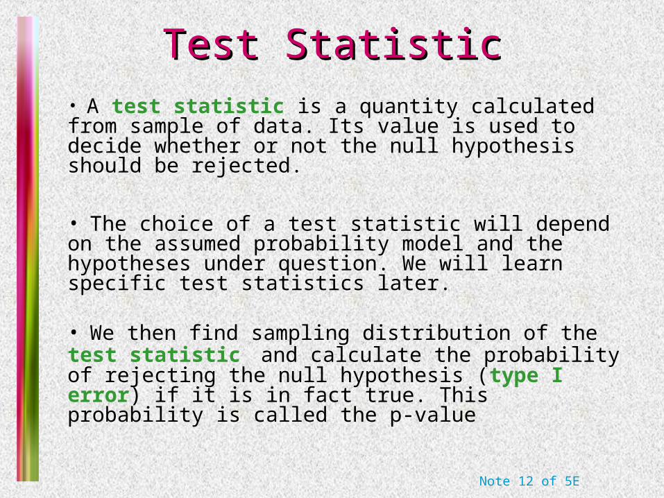
• A test statistic is a quantity calculated from sample of data. Its value is used to decide whether or not the null hypothesis should be rejected.
• The choice of a test statistic will depend on the assumed probability model and the hypotheses under question. We will learn specific test statistics later. • We then find sampling distribution of the test statistic and calculate the probability of rejecting the null hypothesis (type I error) if it is in fact true. This probability is called the p-value

Note 12 of 5E
P-valueP-value• The p-value is a measure of inconsistency between the hypothesized value under the null hypothesis and the observed sample.
• The p-value is the probability, assuming that H0 is true, of obtaining a test statistic value at least as inconsistent with H0 as what actually resulted.
• It measures whether the test statistic is likely or unlikely, assuming H0 is true. Small p-values suggest that the null hypothesis is unlikely to be true. The smaller it is, the more convincing is the rejection of the null hypothesis. It indicates the strength of evidence for rejecting the null hypothesis H0

Note 12 of 5E
DecisionDecisionA decision as to whether H0 should be rejected results from comparing the p-value to the chosen significance level :
– H0 should be rejected if p-value
– H0 should not be rejected if p-value > When p-value>α, state “fail to reject H0” or “not to reject” rather than “accepting H0”. Write “there is insufficient evidence to reject H0”.
Another way to make decision is to use critical value and rejection region, which will not be covered in this class.
Another way to make decision is to use critical value and rejection region, which will not be covered in this class.

Note 12 of 5E
Five Steps of a Statistical TestFive Steps of a Statistical Test
A statistical test of hypothesis consist of five stepsA statistical test of hypothesis consist of five steps
1.1. Specify the Specify the null hypothesisnull hypothesis HH00 and and alternative alternative
hypothesishypothesis HHa a in terms of population parametersin terms of population parameters
2.2. Identify and calculate Identify and calculate test statistictest statistic
3.3. Identify distributionIdentify distribution and find and find p-valuep-value
4. Compare p-value with the given significance level and decide if to reject the null hypothesis
5. State conclusion

Note 12 of 5E
Large Sample Test for Population MeanLarge Sample Test for Population MeanStep 1: Specify the null and alternative hypothesis
– H0: = versus Ha: two-sided test)– H0: = versus Ha: > (one-sided test)– H0: = versus Ha: < one-sided test)
Step 2: Test statistic for large sample (n≥30)
deviation standard andmean size, sample are s and n, where
/
0
x
ns
xz
deviation standard andmean size, sample are s and n, where
/
0
x
ns
xz

Note 12 of 5E
Intuition of the Test StatisticIntuition of the Test Statistic If H0 is true, the value of should be close to 0, and z
will be close to 0. If H0 is false, will be much larger or smaller than 0, and z will be much larger or smaller than 0, indicating that we should reject H0. Thus
xx
Ha:
Ha: >
Ha: <
• z is much larger or smaller than 0 provides evidence against H0 • z is much larger than 0 provides evidence against H0
• z is much smaller than 0 provides evidence against H0
How much larger (or smaller) is large (small) enough?
How much larger (or smaller) is large (small) enough?

Note 12 of 5E
Large Sample Test for Population MeanLarge Sample Test for Population Mean
Step 3: When n is large, the sampling distribution of z will be approximately standard normal under H0.
Compute sample statistic ns
xz
/* 0
ns
xz
/* 0
z is defined for any possible sample. Thus it is a random variable which can take many different values and the sampling distribution tells us the chance of each value. z* is computed from the given data, thus a fixed number.
z is defined for any possible sample. Thus it is a random variable which can take many different values and the sampling distribution tells us the chance of each value. z* is computed from the given data, thus a fixed number.

Note 12 of 5E
Large Sample Test for Population MeanLarge Sample Test for Population Mean
– Ha: < one-sided test)
*)(value-p zzP *)(value-p zzP
– Ha: > (one-sided test)
*)(value-p zzP *)(value-p zzP
|)*|(2
|)*|(|)*|(value-p
zzP
zzPzzP
|)*|(2
|)*|(|)*|(value-p
zzP
zzPzzP
– Ha: (two-sided test)
P(z>|z*|), P(z>z*) and P(z<z*) can be found from the normal tableP(z>|z*|), P(z>z*) and P(z<z*) can be found from the normal table

Note 12 of 5E
ExampleExample The daily yield for a chemical plant has averaged 880
tons for several years. The quality control manager wants to know if this average has changed. She randomly selects 50 days and records an average yield of 871 tons with a standard deviation of 21 tons. Conduct the test using α=.05.
880:H vs880:H a0 880:H vs880:H a0
03.350/21
880871
/*
21s ,871 ,50 ,880
:statisticTest
0
0
ns
xz
xn
03.350/21
880871
/*
21s ,871 ,50 ,880
:statisticTest
0
0
ns
xz
xn

Note 12 of 5E
ExampleExample
0024.)0012(.2)03.3(2value
testsided- twoa is this:value-
zPp
p0024.)0012(.2)03.3(2value
testsided- twoa is this:value-
zPp
p
Decision: since p-value<α, we reject the hypothesis that μ=880.
Conclusion: the average yield has changed and the change is statistically significant at level .05.
In fact, the p-value tells us more: the null hypothesis is very unlikely to be true. If the significance level is set to be any value greater or equal to .0024, we would still reject the null hypothesis. Thus, another interpretation of the p-value is the smallest level of significance at which H0 would be rejected, and p-value is also called the observed significance level.
In fact, the p-value tells us more: the null hypothesis is very unlikely to be true. If the significance level is set to be any value greater or equal to .0024, we would still reject the null hypothesis. Thus, another interpretation of the p-value is the smallest level of significance at which H0 would be rejected, and p-value is also called the observed significance level.

Note 12 of 5E
ExampleExample A homeowner randomly samples 64 homes similar to
her own and finds that the average selling price is $252,000 with a standard deviation of $15,000. Is this sufficient evidence to conclude that the average selling price is greater than $250,000? Use = .01.
000,250:H vs000,250:H a0 000,250:H vs000,250:H a0
07.164/000,15
000,250000,252
/*
:statisticTest
0
ns
xz
07.164/000,15
000,250000,252
/*
:statisticTest
0
ns
xz

Note 12 of 5E
ExampleExample
1423.3577.5.
)07.1(value
testsided-one a is this
:value-
zPp
p
1423.3577.5.
)07.1(value
testsided-one a is this
:value-
zPp
p
Decision: since the p-value is greater than = .01, H0 is not rejected.
Conclusion: there is insufficient evidence to indicate that the average selling price is greater than $250,000.

Note 12 of 5E
Small Sample Test for Population MeanSmall Sample Test for Population MeanStep 1: Specify the null and alternative hypothesis
– H0: = versus Ha: two-sided test)– H0: = versus Ha: > (one-sided test)– H0: = versus Ha: < one-sided test)
Step 2: Test statistic for small sample
deviation standard andmean size, sample are s and n, where
/
0
x
ns
xt
deviation standard andmean size, sample are s and n, where
/
0
x
ns
xt
Step 3: When samples are from a normal population, under H0 , the sampling distribution of t has a Student’s t distribution
with n-1 degrees of freedom

Note 12 of 5E
Small Sample Test for Population MeanSmall Sample Test for Population Mean
Step 3: Find p-value. Compute sample statistic
ns
xt
/* 0
ns
xt
/* 0
– Ha: two-sided test)
– Ha: > (one-sided test)
– Ha: < (one-sided test)
|)*|(2value-p ttP |)*|(2value-p ttP
*)(value-p ttP *)(value-p ttP
*)(value-p ttP *)(value-p ttP
P(t>|t*|), P(t>t*) and P(t<t*) can be found from the t tableP(t>|t*|), P(t>t*) and P(t<t*) can be found from the t table

Note 12 of 5E
ExampleExample
A sprinkler system is designed so that the average time for the sprinklers to activate after being turned on is no more than 15 seconds. A test of 5 systems gave the following times:
17, 31, 12, 17, 13, 25 Is the system working as specified? Test using = .05.
specified) as ng(not worki 15:H
specified) as (working 15:H
a
0
specified) as ng(not worki 15:H
specified) as (working 15:H
a
0

Note 12 of 5E
ExampleExampleData:Data: 17, 31, 12, 17, 13, 25
First, calculate the sample mean and standard deviation.
387.75
6115
2477
1
)(
167.196
115
222
nnx
xs
n
xx i
387.75
6115
2477
1
)(
167.196
115
222
nnx
xs
n
xx i
5161 38.16/387.7
15167.19
/*
:freedom of Degrees :statisticTest
0
ndfns
xt
5161 38.16/387.7
15167.19
/*
:freedom of Degrees :statisticTest
0
ndfns
xt

Note 12 of 5E
Approximating the p-valueApproximating the p-value Since the sample size is small, we need to assume a
normal population and use t distribution. We can only approximate the p-value for the test using Table 4.
Since the observed value of t* = 1.38 is smaller than t.10 = 1.476,
p-value > .10.

Note 12 of 5E
ExampleExample
Decision: since the p-value is greater than .1, than it is greater than = .05, H0 is not rejected.
Conclusion: there is insufficient evidence to indicate that the average activation time is greater than 15 seconds.
Exact p-values can be calculated by computers.

Note 12 of 5E
Large Sample Test for Difference Between Large Sample Test for Difference Between Two Population MeansTwo Population Means
. varianceand mean with 1 population
fromdrawn size of sample randomA 211
1
μ
n
. varianceand mean with 1 population
fromdrawn size of sample randomA 211
1
μ
n
. varianceand mean with 2 population
fromdrawn size of sample randomA 222
2
μ
n
. varianceand mean with 2 population
fromdrawn size of sample randomA 222
2
μ
n

Note 12 of 5E
Large Sample Test for Difference Between Large Sample Test for Difference Between Two Population MeansTwo Population Means
Step 1: Specify the null and alternative hypothesis
– H0: D0versus Ha: D
two-sided test)– H0: D0versus Ha: D
(one-sided test)– H0: D0versus Ha: D
one-sided test)
where D0 is some specified difference that you wish to test. D0=0 when testing no difference.

Note 12 of 5E
Large Sample Test for Difference Between Large Sample Test for Difference Between Two Population MeansTwo Population Means
Step 2: Test statistic for large sample sizes when
n1≥30 and n2≥30
2
22
1
21
021
ns
ns
Dxxz
2
22
1
21
021
ns
ns
Dxxz
Step 3: Under H0, the sampling distribution of z is approximately standard normal

Note 12 of 5E
Large Sample Test for Difference Between Large Sample Test for Difference Between Two Population MeansTwo Population Means
Step 3: Find p-value. Compute
– Ha: Dtwo-sided test)
– Ha: D(one-sided test)
– Ha: D(one-sided test)
|)*|(2value-p zzP |)*|(2value-p zzP
2
22
1
21
021*
ns
ns
Dxxz
2
22
1
21
021*
ns
ns
Dxxz
*)(value-p zzP *)(value-p zzP
*)(value-p zzP *)(value-p zzP

Note 12 of 5E
ExampleExample
• Is there a difference in the average daily intakes of dairy products for men versus women? Use = .05.
Avg Daily Intakes Men Women
Sample size 50 50
Sample mean 756 762
Sample Std Dev 35 30
(same) 0:H 210
2
22
1
21
21 0*
:statisticTest
ns
ns
xxz
)(different 0:H 21a
92.
5030
5035
076275622
Note 12 of 5E
ExampleExample
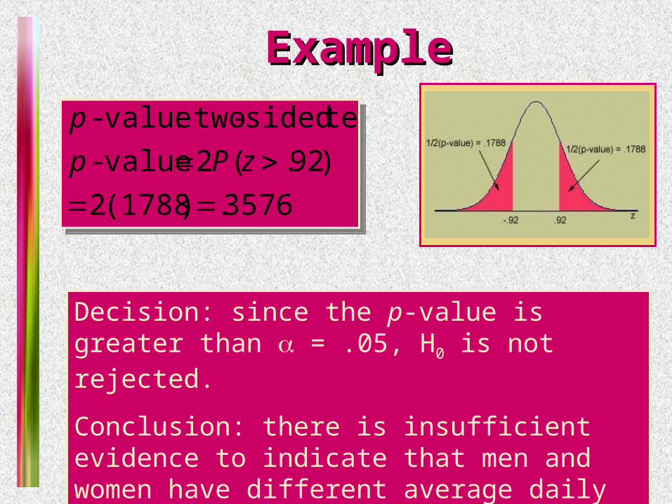
3576.)1788(.2
)92.(2value-
testsided- two:value-
zPp
p
3576.)1788(.2
)92.(2value-
testsided- two:value-
zPp
p
Decision: since the p-value is greater than = .05, H0 is not rejected.
Conclusion: there is insufficient evidence to indicate that men and women have different average daily intakes.

Note 12 of 5E
Small Sample Testing the Difference Small Sample Testing the Difference between Two Population Meansbetween Two Population Means
. varianceand mean with
on distributi normal with 1 population
fromdrawn size of sample randomA
21
1
μ
n
. varianceand mean with
on distributi normal with 1 population
fromdrawn size of sample randomA
21
1
μ
n
. varianceand mean with
on distributi normal with 2 population
fromdrawn size of sample randomA
22
2
μ
n
. varianceand mean with
on distributi normal with 2 population
fromdrawn size of sample randomA
22
2
μ
n
Note that both population are normally distributed with the same variances

Note 12 of 5E
Small Sample Testing the Difference Small Sample Testing the Difference between Two Population Meansbetween Two Population Means
Step 1: Specify the null and alternative hypothesis
– H0: D0versus Ha: D
two-sided test)– H0: D0versus Ha: D
(one-sided test)– H0: D0versus Ha: D
one-sided test)
where D0 is some specified difference that you wish to test. D0=0 when testing no difference.

Note 12 of 5E
Small Sample Testing the Difference Small Sample Testing the Difference between Two Population Meansbetween Two Population Means
Step 2: Test statistic for small sample sizes
2
)1()1(s as calculated is where
11
21
222
21122
21
021
nn
snsns
nns
Dxxt
2
)1()1(s as calculated is where
11
21
222
21122
21
021
nn
snsns
nns
Dxxt
Step 3: Under H0, the sampling distribution of t has a Student’s t distribution with n1+n2-2 degrees of freedom

Note 12 of 5E
Small Sample Testing the Difference Small Sample Testing the Difference between Two Population Meansbetween Two Population Means
Step 3: Find p-value. Compute
– Ha: Dtwo-sided test)
– Ha: D(one-sided test)
– Ha: D(one-sided test)
|)*|(2value-p ttP |)*|(2value-p ttP
*)(value-p ttP *)(value-p ttP
*)(value-p ttP *)(value-p ttP
11
*
21
021
nns
Dxxt
11*
21
021
nns
Dxxt

Note 12 of 5E
ExampleExample Two training procedures are compared by
measuring the time that it takes trainees to assemble a device. A different group of trainees are taught using each method. Is there a difference in the two methods? Use = .01.
Time to Assemble
Method 1 Method 2
Sample size 10 12
Sample mean 35 31
Sample Std Dev
4.9 4.5
0:H 210
21
2
21
11
0
:statisticTest
nns
xxt
0:H 21a

Note 12 of 5E
ExampleExampleTime to Assemble
Method 1 Method 2
Sample size 10 12
Sample mean 35 31
Sample Std Dev
4.9 4.5
99.1
121
101
942.21
3135*
:statisticTest
t
942.2120
)5.4(11)9.4(9
2
)1()1(
:Calculate
22
21
222
2112
nn
snsns

Note 12 of 5E
ExampleExample
1.value05.05.)99.1(025.
)99.1(2value- sided- two:value-
ptP
tPpp1.value05.05.)99.1(025.
)99.1(2value- sided- two:value-
ptP
tPpp
Decision: since the p-value is greater than = .01, H0 is not rejected.
Conclusion: there is insufficient evidence to indicate a difference in the population means.
Decision: since the p-value is greater than = .01, H0 is not rejected.
Conclusion: there is insufficient evidence to indicate a difference in the population means.
df = n1 + n2 – 2 = 10 + 12 – 2 = 20df = n1 + n2 – 2 = 10 + 12 – 2 = 20

Note 12 of 5E
The Paired-Difference TestThe Paired-Difference Test• We have assumed that samples from two populations are independent. Sometimes the assumption of independent samples is intentionally violated, resulting in a matched-pairsmatched-pairs or paired-difference testpaired-difference test.• By designing the experiment in this way, we can eliminate unwanted variability in the experiment • Denote data as
Pair 1 2 … n
Population 1 x11 x12 … x1n
Population 2 x21 x22 … x2n
Difference d1= x11- x21 d2=x12- x22 … dn=x1n- x2n

Note 12 of 5E
The Paired-Difference TestThe Paired-Difference Test
Step 1: Specify the null and alternative hypothesis
– H0: D0versus Ha: D
two-sided test)– H0: D0versus Ha: D
(one-sided test)– H0: D0versus Ha: D
one-sided test)
where D0 is some specified difference that you wish to test. D0=0 when testing no difference.

Note 12 of 5E
The Paired-Difference TestThe Paired-Difference Test
Step 2: Test statistic for small sample sizes
n
d
d
dd
sd
ns
Ddt
,, sdifference paired theofdeviation
standard andmean sample are and where
/
1
0
n
d
d
dd
sd
ns
Ddt
,, sdifference paired theofdeviation
standard andmean sample are and where
/
1
0
Step 3: Under H0, the sampling distribution of t has a Student’s t distribution with n-1 degrees of freedom

Note 12 of 5E
The Paired-Difference TestThe Paired-Difference Test
Step 3: Find p-value. Compute
– Ha: Dtwo-sided test)
– Ha: D(one-sided test)
– Ha: D(one-sided test)
|)*|(2value-p ttP |)*|(2value-p ttP
*)(value-p ttP *)(value-p ttP
*)(value-p ttP *)(value-p ttP
/
* 0
ns
Ddt
d
/* 0
ns
Ddt
d

Note 12 of 5E
Paired t Test ExamplePaired t Test Example
A weight reduction center advertises that participants in its program lose an average of at least 5 pounds during the first week of the participation. Because of numerous complaints, the state’s consumer protection agency doubts this claim. To test the claim at the 0.05 level of significance, 12 participants were randomly selected. Their initial weights and their weights after 1 week in the program appear on the next slide. Set up and perform an appropriate hypothesis test.

Note 12 of 5E
Paired Sample ExamplePaired Sample Example continuedcontinued
Member Initial
Weight One Week
Weight Difference Initial -1week
1 195 195 0
2 153 151 2
3 174 170 4
4 125 123 2
5 149 144 5
6 152 149 3
7 135 131 4
8 143 147 -4
9 139 138 1
10 198 192 6
11 215 211 4
12 153 152 1

Note 12 of 5E
Paired Sample ExamplePaired Sample Example continuedcontinued
Each member serves as his/her own pair. weight changes=initial weight–weight after one week
claimed) as ng(not worki 5:H
claimed) as (working 5:H
21a
210
claimed) as ng(not worki 5:H
claimed) as (working 5:H
21a
210
111121
45.312/674.2
5333.2
/*
2.674s 2.333,d 12,n
0
d
ndf
ns
Ddt
d
111121
45.312/674.2
5333.2
/*
2.674s 2.333,d 12,n
0
d
ndf
ns
Ddt
d

Note 12 of 5E
Paired Sample ExamplePaired Sample Example continuedcontinued
005.value- sided-one :value- pp 005.value- sided-one :value- pp
Decision: since the p-value is smaller than = .05, H0 is rejected.
Conclusion: there is strong evidence that the mean weight loss is less than 5 pounds for those who took the program for one week.
Decision: since the p-value is smaller than = .05, H0 is rejected.
Conclusion: there is strong evidence that the mean weight loss is less than 5 pounds for those who took the program for one week.

Note 12 of 5E
Key ConceptsKey Concepts
I. I. A statistical test of hypothesis consist of five stepsA statistical test of hypothesis consist of five steps
1.1. Specify the Specify the null hypothesisnull hypothesis HH00 and and alternative alternative
hypothesishypothesis HHa a in terms of population parametersin terms of population parameters
2.2. Identify and calculate Identify and calculate test statistictest statistic
3.3. Identify distributionIdentify distribution and find and find p-valuep-value
4. Compare p-value with the given significance level and decide if to reject the null hypothesis
5. State conclusion

Note 12 of 5E
Key ConceptsKey ConceptsII.II. Errors and Statistical Significance Errors and Statistical Significance
1. Type I error: reject the null hypothesis when it is true
2. Type II error: fail to reject the null hypothesis when it is false
3. The significance level = P(type I error)
4 =P(type II error)
5. The p-value is the probability of observing a test statistic as extreme as or more than the one observed; also, the smallest value of for which H 0 can be rejected
6. When the p-value is less than the significance level , the null hypothesis is rejected

Note 12 of 5E
Key ConceptsKey Concepts
III.III. Test for a population mean Test for a population mean HH00: : µ=µµ=µ00
ns
xz
/0
ns
xz
/0
Sample size?
Ha: µ≠µ0
p-value=
2P(z>|z*|)
Ha: µ>µ0
p-value=
P(z>z*)
Ha: µ<µ0
p-value=
P(z<z*)
Ha: µ≠µ0
p-value=
2P(t>|t*|)
Ha: µ>µ0
p-value=
2P(t>t*)
Ha: µ≠µ0
p-value=
P(t<t*)
ns
xt
/0
ns
xt
/0
large small

Note 12 of 5E
Key ConceptsKey Concepts
IV. Test for Difference Between Two IV. Test for Difference Between Two Population MeanPopulation Mean H H00: : µµ11-µ-µ22=D=D00
Sample size?
Ha: µ1-µ2≠D0
p-value=
2P(z>|z*|)
Ha: µ1-µ2>D0
p-value=
P(z>z*)
Ha: µ1-µ2<D0
p-value=
P(z<z*)
Ha:µ1-µ2≠D0
p-value=
2P(t>|t*|)
Ha: µ1-µ2>D0
p-value=
2P(t>t*)
Ha: µ1-µ2<D0
p-value=
P(t<t*)
large small
2
22
1
21
021
ns
ns
Dxxz
2
22
1
21
021
ns
ns
Dxxz
21
021
11
nns
Dxxt
21
021
11
nns
Dxxt

Note 12 of 5E
Key ConceptsKey Concepts
V. The Paired-Difference TestV. The Paired-Difference Test
ns
Ddt
d /
0
ns
Ddt
d /
0
– Ha: Dtwo-sided test)
– Ha: D(one-sided test)
– Ha: D(one-sided test)
|)*|(2value-p ttP |)*|(2value-p ttP
*)(value-p ttP *)(value-p ttP
*)(value-p ttP *)(value-p ttP