northern watch 2008 above-water sensor trials at the...
TRANSCRIPT

Northern Watch 2008 Above-Water Sensor Trials at the Naval Electronic Systems Test Range Atlantic NESTRA Experimental Set-up, Analysis, and Results for the Radar
Dan Brookes DRDC – Ottawa Research Centre
Defence Research and Development Canada Scientific Report DRDC-RDDC-2017-R156 October 2017

IMPORTANT INFORMATIVE STATEMENTS Disclaimer: Her Majesty the Queen in Right of Canada (Department of National Defence) makes no representations or warranties, express or implied, of any kind whatsoever, and assumes no liability for the accuracy, reliability, completeness, currency or usefulness of any information, product, process or material included in this document. Nothing in this document should be interpreted as an endorsement for the specific use of any tool, technique or process examined in it. Any reliance on, or use of, any information, product, process or material included in this document is at the sole risk of the person so using it or relying on it. Canada does not assume any liability in respect of any damages or losses arising out of or in connection with the use of, or reliance on, any information, product, process or material included in this document. This document was reviewed for Controlled Goods by Defence Research and Development Canada (DRDC) using the Schedule to the Defence Production Act. Endorsement statement: This publication has been peer-reviewed and published by the Editorial Office of Defence Research and Development Canada, an agency of the Department of National Defence of Canada. Inquiries can be sent to: [email protected]. Work sponsored by Project 06AB1: Northern Watch (formerly 15ej01)
Template in use: (2003) SR Advanced Template_EN (051115).dot
© Her Majesty the Queen in Right of Canada (Department of National Defence), 2017
© Sa Majesté la Reine en droit du Canada (Ministère de la Défence nationale), 2017

DRDC-RDDC-2017-R156 i
Abstract
In August 2008 a team of scientists and technicians from DRDC attempted to undertake the first Arctic field trials for the Northern Watch Technology Demonstration Program (TDP) project on Devon Island at sites in Gascoyne Inlet and on Cape Liddon. Key objectives of the operation were to deploy several above water sensor (AWS) systems on Cape Liddon and an underwater sensor (UWS) system in Barrow Strait. The aim was to evaluate their individual and collective ability to detect, track, classify and identify a cooperative vessel, or targets of opportunity. Very severe weather prevented the accomplishment of this objective, so alternative trials were arranged for the AWS at the Naval Electronic Systems Test Range Atlantic (NESTRA) near Halifax in 7–11 Dec. 2008. The main intent was to perform a comprehensive shake down of all the AWS systems and perform as many of the original Arctic system tests as possible under the constraints imposed by this southern site. This report is one of several that are anticipated to result from the analyses of the NESTRA Trials data for each of the main AW sensors; this one is focused primarily on the performance of the navigation radar system. The results of the radar data analysis were generally consistent with performance predicted by the Scenario/Shipboard Integrated Environment for Tactics and Awareness (SIESTA) for the environmental conditions and the target-sensor geometries. The CFAV Quest was tracked to a maximum distance (stern-, or bow-on) about 29 km; large container vessels were tracked up to 35 km; and small vessels were tracked to distances of 10 to 20 km. The main factor limiting the radar’s ability to track ships was the line of sight to the horizon. The indications were that this radar system would be suitable for further evaluation at the arctic trials site near Gascoyne Inlet.
Significance to Defence and Security
Background: With recent and anticipated changes in arctic climate, more shipping channels in the Canadian Arctic Archipelago are opening during the summer, and for longer periods of time. This, coupled with increased interest in exploiting northern resources, has led to a re-examination of the need for greater monitoring of, and presence in, the Arctic; the Northern Watch (NW) Technology Demonstration Program (TDP) project was initiated to support this research. Part of the original mandate of the NW project was to develop, and demonstrate, a prototype suite of integrated, complementary sensor systems for effective surveillance of surface vessel traffic at a known arctic maritime chokepoint. The system-of-systems would also be capable of limited surveillance of underwater vessels and local aircraft. Within budget constraints, the component sensors were selected based on their complementary capabilities to detect, track, classify and identify vessels of interest. The primary systems for maritime domain awareness consisted of both above water (AW) and underwater (UW) systems. The AWS systems consisted of commercial-off-the-shelf (COTS) devices, as well as systems developed by, or specifically for, Defence R&D Canada (DRDC). The COTS systems included the Rutter 100S6 X-band navigation radar, and an Automatic Identification System (AIS) receiver, whereas the DRDC systems included an in-house developed radar warning receiver (RWR), and an electro-optic/infrared imaging (camera) system developed for DRDC using COTS components. The UW sensor system was a passive sensor array based on an earlier DRDC demonstration system called the Rapidly Deployable System (RDS).

ii DRDC-RDDC-2017-R156
Developing the integrated suite was to be accomplished by iterative integration and refinement over the duration of the project, culminating with a complete system demonstration in the final year. The first step of the process was to simultaneously evaluate the capabilities of the individual stand-alone systems under identical conditions at the arctic trials site—Gascoyne Inlet (GI) and Cape Liddon (CL) overlooking Barrow Strait—during the main arctic shipping season. However, these first sensor trials in August of 2008 had to be aborted after two weeks of severe weather that prevented the deployment of both the AW and UW sensors and their associated infrastructure. Subsequently, alternative trials were arranged for the AWS at the Naval Electronic Systems Test Range Atlantic (NESTRA) near Halifax during 7–11 Dec. 2008. The intent was to perform a comprehensive shake-down of all the AWS and perform as many of the original arctic system tests as possible under the constraints imposed by this southern site. The trials also served as a very useful team building exercise by providing the first real opportunity for the multi-centre, multi-disciplinary, scientific team to work together in an operational setting.
In addition to the sensor systems and associated shelters, the resources required for the trials included the NESTRA facilities (power, lab space, and meeting rooms), and cooperative targets provided by the Canadian Forces Auxiliary Vessel (CFAV) Quest and her Rigid Hull Inflatable Boat (RHIB). The location near the entrance to the Halifax harbour also provided a wide selection of targets of opportunity, from small fishing vessels to large container ships.
Results: An extensive database of sensor data was acquired from all of the AWS systems, including data from calibrated targets, and positional “truth” of most vessels recorded from Global Position Systems (GPS) or reported via ship’s Automatic Identification System (AIS). Environmental data (e.g., weather, sea state) were also acquired from local weather stations and provided by imagery recorded during the trials. With respect to the radar system, this data was used to provide a preliminary evaluation of the system’s capability under conditions very similar to those experienced at GI earlier in August 2008. The radar’s detection and tracking capabilities were consistent with predictions provided by software developed by DRDC called Shipborne/Scenario Integrated Environment for Tactics and Awareness (SIESTA).
It was also discovered that, under certain conditions, the Rutter 100S6 radar system could be used as a rudimentary RWR to detect and provide bearing tracks on vessels that were using similar X-band navigation radars.
Significance: These trials provided the first real opportunity for DRDC to test the radar system, and become familiar with its functioning under challenging operational conditions. The added benefits of co-testing the other AWS systems under identical conditions, becoming familiar with the large scale logistics required for such trials, and the team building opportunity, were essential to the future success of the arctic field trials specifically, and of the project in general. The radar results from these trials supported the belief that a non-coherent 25 kW peak-power radar system, such as the Rutter 100S6, deployed to the top of Cape Liddon at a height of 320 m above mean sea level might be capable of detecting and tracking medium to large ships up to the full distance (~70 km) across Barrow Strait choke-point.
Also, with the belief that it would be useful for developing new target detection, tracking, classification and identification algorithms, and new sensor integration concepts, the database collected from all of the sensors and supporting systems was later shared amongst the participants of SEN TP-1, the technical panel (TP) responsible for Sensor Integration research within The

DRDC-RDDC-2017-R156 iii
Technical Cooperation Program (TTCP). TTCP member nations include Canada, the United States, the United Kingdom, Australia and New Zealand.
Future plans: Follow-on work will involve further analysis of the NESTRA data from all of the AW systems (individually and collectively) to aid in the development of system integration concepts. Additional system trials and evaluations are also anticipated to be performed in the south and at the arctic test site. In the near term, specifically with respect to the radar, additional trials in the south are planned in order to determine its stand-alone system capability for detecting and tracking aircraft.

iv DRDC-RDDC-2017-R156
Résumé
En août 2008, une équipe de scientifiques et de techniciens de RDDC a voulu mener en Arctique, plus précisément à Gascoyne Inlet et Cap Liddon, sur l’île Devon, les premiers essais sur le terrain du Projet de démonstration de technologies Surveillance du Nord (PDT NW). Cette opération visait principalement à déployer plusieurs systèmes de capteurs au-dessus de la surface (AWS) à Cap Liddon et un système de capteurs sous-marins (UWS) au détroit de Barrow, afin d’évaluer leur utilité collective et individuelle à détecter, poursuivre, classifier et identifier un navire ami ou des objectifs inopinés. Comme des conditions météorologiques extrêmes ont empêché d’atteindre cet objectif, on a plutôt tenu du 7 au 11 décembre 2008 des essais des systèmes AWS au Centre d’essai des systèmes électroniques naval de l’Atlantique (NESTRA), près d’Halifax. Ils ont surtout visé à faire des essais exhaustifs des systèmes AWS et de mener autant des tests prévus en environnement arctique que l’a permis ce site plus éloigné du pôle. Le présent rapport est le premier de plusieurs prévus sur les analyses des données des essais NESTRA visant chacun des principaux capteurs de surface, et il porte surtout sur les performances du système radar de navigation. Les résultats de cette analyse concordent en gros avec les performances prévues selon un scénario du système embarqué d’environnement intégré de tactique et de connaissance de la situation (SIESTA), dans les conditions environnementales et avec la configuration des cibles et des capteurs simulées. On a poursuivi le NAFC Quest jusqu’à une distance maximale de 29 km, de poupe ou de proue; des grand navires transporteurs de conteneurs, jusqu’à 35 km; et des navires plus petits, de 10 à 20 km. Le facteur déterminant dans la capacité de poursuite du radar s’est révélé être la visibilité jusqu’à la ligne d’horizon. Ces essais indiquent que ce système radar se prêterait bien à des essais plus poussés au site d’essai arctique près de Gascoyne Inlet.
Importance pour la défense et la sécurité
Contexte: Vu les changements observés et prévus au climat de l’Arctique, les voies maritimes dans l’archipel Arctique du Canada se multiplient pendant l’été et restent ouvertes plus longtemps. En parallèle avec un intérêt accru d’exploiter les ressources naturelles du Nord, cela a mené à réévaluer le besoin d’une surveillance et d’une présence accrue dans l’Arctique; le Projet de démonstration de technologies Surveillance du Nord (NW) vise à appuyer ces recherches. L’un des mandats de ce projet était d’élaborer puis de faire la démonstration du prototype d’un ensemble de systèmes de capteurs intégrés et complémentaires afin de surveiller les navires de surface à un goulot d’étranglement maritime connu. Ce système de systèmes devait aussi pouvoir jusqu’à un certain point surveiller les sous-marins et les aéronefs locaux. En respectant les contraintes budgétaires, les composantes ont été choisies en fonction de leurs capacités complémentaires de détecter, poursuivre, classifier et identifier les navires ciblés. Les principaux systèmes choisis pour la connaissance du domaine maritime consistaient tant en systèmes de surface (AW) que sous-marins (UW). Les systèmes AW consistait en appareils commerciaux, et en systèmes développés par, ou spécifiquement pour, Recherche et développement pour la Défense Canada (RDDC). Les systèmes commercial comportait notamment le radar de navigation en bande X Rutter 100S6 et un récepteur de système d’identification automatique (AIS), et les systèmes de RDDC comptaient notamment un Récepteur d’alerte radar (RWR) développé à

DRDC-RDDC-2017-R156 v
l’interne et un système d’imagerie (une caméra) électro-optique infrarouge développée pour RDDC à partir de composantes commerciales. Le système sous-marin était un réseau de capteurs passifs fondé sur un système de démonstration antérieur du RDDC nommé le « système rapidement déployable » (RDS).
Élaborer la suite intégrée devait résulter de l’intégration et du perfectionnement itératifs au cours du projet, afin de pouvoir, la dernière année, faire la démonstration d’un système complet. Première étape : évaluer en parallèle les capacités des systèmes distincts dans des conditions environnementales identiques aux sites d’essai arctiques, c’est-à-dire Gascoyne Inlet (GI) et Cap Liddon (CL), au-dessus du détroit de Barrow, pendant la saison de navigation en arctique. Il a toutefois fallu abandonner ces premiers essais d’août 2008, car des conditions météorologiques extrêmes pendant deux semaines ont empêché le déploiement des capteurs de surface et sous-marins et de l’infrastructure connexe. Par conséquent, des essais d’appoint des capteurs de surface ont eu lieu du 7 au 11 décembre 2008, au Centre d’essai des systèmes électroniques naval de l’Atlantique (NESTRA), près d’Halifax. Ils ont visé à faire des essais exhaustifs des systèmes AWS et de mener autant des tests prévus en environnement arctique que l’a permis ce site plus éloigné du pôle. Ils ont aussi servi d’exercice très utile de renforcement de l'esprit d'équipe, car ce fut la première occasion pour l’équipe scientifique pluridisciplinaire et provenant de plusieurs centres de travailler ensemble dans un contexte opérationnel.
Outre les systèmes de capteurs et les abris connexes, les ressources nécessaires aux essais ont comporté les installations du NESTRA (alimentation électrique, laboratoires et salles de réunion), et des cibles coopératives : le navire auxiliaire des Forces canadiennes (NAFC) Quest et son embarcation pneumatique à coque rigide (RHIB). L’emplacement du NESTRA, près du port d’Halifax, a aussi permis de poursuivre un grand nombre d’objectifs inopinés; allant des petits bateaux de pêche à des grands navires transporteurs de conteneurs.
Résultats: Les systèmes de capteurs de surface ont produit une grande quantité de données, notamment des données de cibles calibrées, et l’emplacement « réel » de la plupart des navires, enregistré à partir de systèmes GPS ou transmis par le système d’identification automatique (AIS) du navire. Les données environnementales, comme les conditions météorologiques et l’état de la mer, ont été enregistrées à partir des stations météo locales et fournies par images acquises pendant les essais. Pour le système radar, ces données ont permis de faire une évaluation préliminaire des capacités du système dans des conditions très proches de celles observées plus tôt à Gascoyne Inlet, en août 2008. Les capacités mesurées de détection et de poursuite du radar se sont révélées comparables à celles prévues par un logiciel de simulation développé par RDDC nommé le Système embarqué d’environnement intégré de tactique et de connaissance de la situation (SIESTA).
On a aussi découvert que le système radar Rutter 100S6 peut, dans certaines conditions, servir de récepteur d’alerte radar rudimentaire, et ainsi détecter et indiquer la direction (à savoir la piste d'azimuts) de navires qui émettent en utilisant des radars de navigation en bande X semblables.
Importance: Ces essais ont donné à RDDC la première occasion concrète de mettre à l’essai ce système radar et se familiariser avec son fonctionnement en conditions opérationnelles difficiles. Les avantages connexes, soit la mise à l’essai simultanée d’autres systèmes AWS dans des conditions identiques, l’expérience acquise dans la logistique d’envergure nécessaire pour ces essais, et l’exercice de renforcement de l'esprit d'équipe, se sont révélés essentiels à la réussite

vi DRDC-RDDC-2017-R156
tant des essais subséquents en Arctique en particulier que de façon plus générale du projet complet. Les résultats de ces essais radar appuient l’opinion qu’un système radar non cohérent d’une puissance de crête de 25 kW, comme le Rutter 100S6, déployé au sommet du Cap Liddon (320 m au-dessus du niveau moyen de la mer), serait en mesure de détecter et de poursuivre les navires de dimensions moyennes et les gros navires jusqu’à la distance totale (70 km environ) dans le goulet d'étranglement du détroit de Barrow.
En outre, l’équipe a pensé que la base des données recueillies de tous les capteurs et les systèmes de soutien serait utile au développement de nouveaux algorithmes de détection, poursuite, classification et identification des cibles ainsi que de nouveaux concepts d’intégration des capteurs; elle l’a donc rendue accessible aux participants de SEN TP-1, le groupe d’experts chargé de la recherche en intégration des capteurs du Programme de coopération technique (TTCP). Parmi les pays membres du TTCP, on compte le Canada, les États-Unis, le Royaume-Uni, l’Australie et la Nouvelle-Zélande.
Recherches futures: Les travaux subséquents porteront sur d’autres analyses des données tirées des essais NESTRA provenant de tous les systèmes de surface, séparément et en groupe, afin d’aider à l’élaboration de concepts d’intégration de systèmes. D’autres essais et évaluations des systèmes sont prévus tant au site d’essai de l’Arctique que plus au sud. À court terme, plus précisément au sujet du radar, d’autres essais sont prévus ailleurs qu’en Arctique afin d’évaluer sa capacité à détecter et poursuivre les aéronefs.

DRDC-RDDC-2017-R156 vii
Table of Contents
Abstract . . . . . . . . . . . . . . . . . . . . . . . . . . . . . . . . . i Significance to Defence and Security . . . . . . . . . . . . . . . . . . . . . . i Résumé . . . . . . . . . . . . . . . . . . . . . . . . . . . . . . . . iv
Importance pour la défense et la sécurité . . . . . . . . . . . . . . . . . . . . iv
Table of Contents . . . . . . . . . . . . . . . . . . . . . . . . . . . . vii List of Figures . . . . . . . . . . . . . . . . . . . . . . . . . . . . . ix
List of Tables . . . . . . . . . . . . . . . . . . . . . . . . . . . . . . xix
Acknowledgements . . . . . . . . . . . . . . . . . . . . . . . . . . . xx
1 Introduction . . . . . . . . . . . . . . . . . . . . . . . . . . . . . 1
2 Sensor Selection Rationale . . . . . . . . . . . . . . . . . . . . . . . 7
2.1 RADARSAT-2, RADARSAT Constellation Mission (RCM) and Space-Based AIS 11
2.2 The North Warning System . . . . . . . . . . . . . . . . . . . . . 12
2.3 Low Cost Marine Navigation Radars for Arctic Surveillance. . . . . . . . . 14
2.4 High Frequency Surface Wave Radar (HFSWR) . . . . . . . . . . . . . 21
2.5 Airborne Radar Systems and Platforms . . . . . . . . . . . . . . . . 23
3 Scientific Objectives . . . . . . . . . . . . . . . . . . . . . . . . . . 25
3.1 Trials Objectives . . . . . . . . . . . . . . . . . . . . . . . . . 26
4 Experimental Equipment Setup . . . . . . . . . . . . . . . . . . . . . . 29
4.1.1 Radar Data Collection Plan . . . . . . . . . . . . . . . . . . 36
4.1.1.1 Radar Calibration . . . . . . . . . . . . . . . . . . 36
5 SIESTA Radar Performance Prediction for NESTRA . . . . . . . . . . . . . 42
6 Data Collection and Analysis . . . . . . . . . . . . . . . . . . . . . . 46
6.1 Results . . . . . . . . . . . . . . . . . . . . . . . . . . . . 46
6.1.1 Environmental Data . . . . . . . . . . . . . . . . . . . . . 46
6.1.2 AIS Data Collection and Analysis . . . . . . . . . . . . . . . . 55
6.1.3 Radar Data Collection and Analysis . . . . . . . . . . . . . . . 75
6.1.3.1 Results of the Rutter 100S6 Radar Post Processing . . . . . . 77
6.1.4 Power Consumption . . . . . . . . . . . . . . . . . . . . . 95
6.1.5 Sigma S6 Radar as a Radar Warning Receiver (RWR) . . . . . . . . 96
7 Observations and Conclusions . . . . . . . . . . . . . . . . . . . . . 102
References . . . . . . . . . . . . . . . . . . . . . . . . . . . . . . 105
Planned CFAV Quest Course Waypoints . . . . . . . . . . . . . . 113 Annex A Rutter 100S6 Radar System Description and Specifications . . . . . . . . 115 Annex B Trials Notes and Data Files . . . . . . . . . . . . . . . . . . . . 120 Annex C

viii DRDC-RDDC-2017-R156
Typical Marine Vessel Traffic observed in the NWP 2003–2008 . . . . . . 124 Annex D Typical East Coast Fishing Boats . . . . . . . . . . . . . . . . . 140 Annex E
List of Symbols/Abbreviations/Acronyms/Initialisms . . . . . . . . . . . . . . 142

DRDC-RDDC-2017-R156 ix
List of Figures
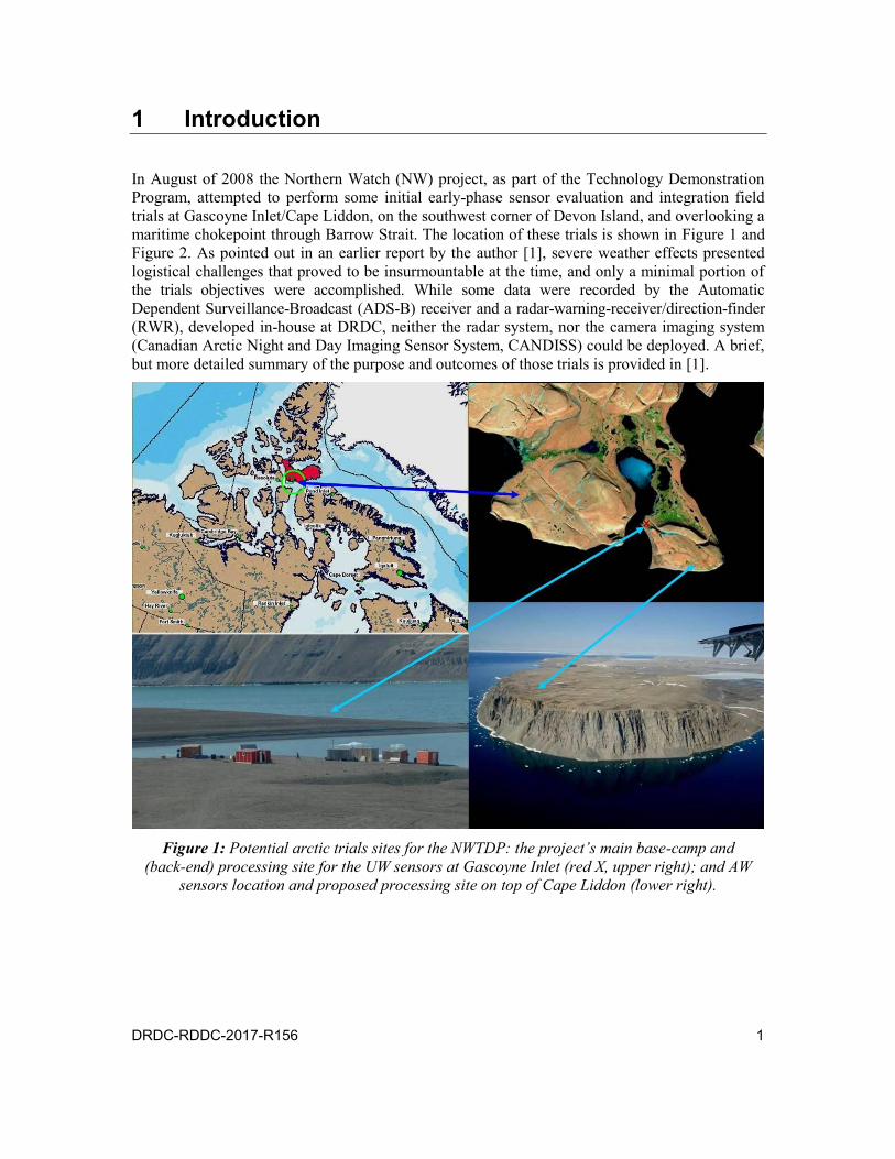
Figure 1: Potential arctic trials sites for the NWTDP: the project’s main base-camp and (back-end) processing site for the UW sensors at Gascoyne Inlet (red X, upper right); and AW sensors location and proposed processing site on top of Cape Liddon (lower right). . . . . . . . . . . . . . . . . . . . . . . . . 1
Figure 2: An aerial perspective of the arctic trials sites based on a photo taken in 2008 by Mr. Nelson McCoy. Radstock Bay, and Gascoyne Inlet were coloured light blue in order to provide a higher land-sea contrast; sea ice is visible in the foreground. . . . . . . . . . . . . . . . . . . . . . . . . . . . 2
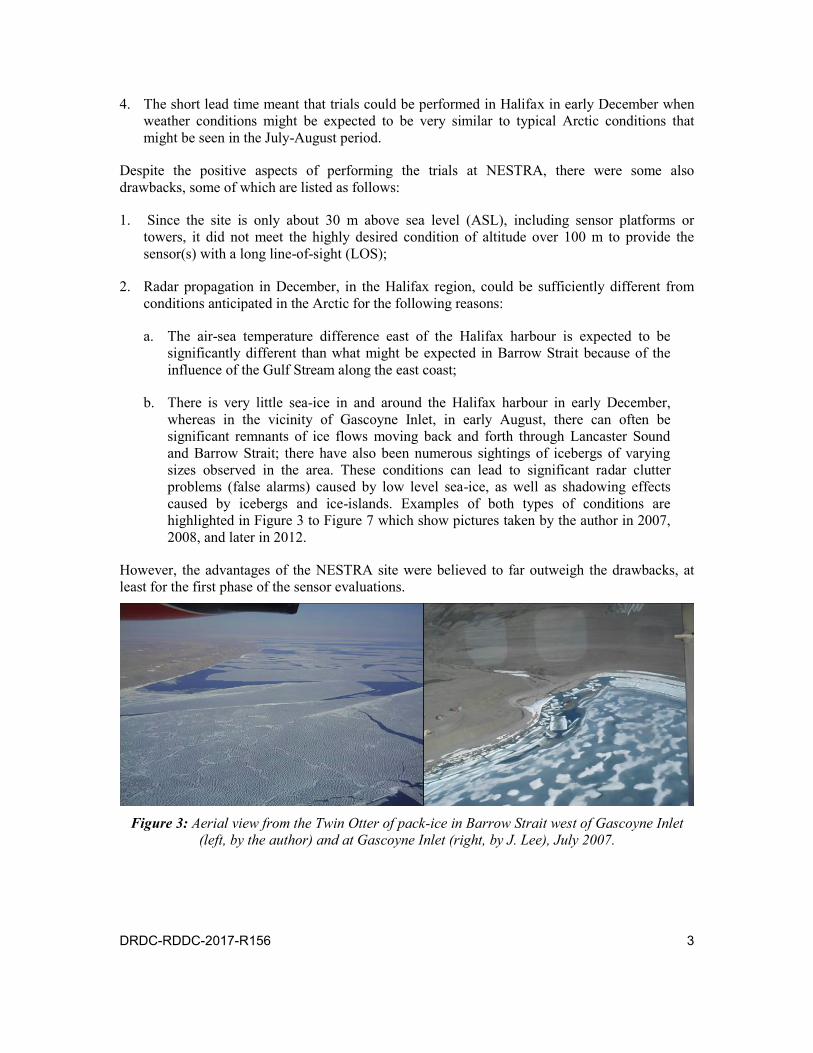
Figure 3: Aerial view from the Twin Otter of pack-ice in Barrow Strait west of Gascoyne Inlet (left, by the author) and at Gascoyne Inlet (right, by J. Lee), July 2007. . . . . . . . . . . . . . . . . . . . . . . . . . . . . 3
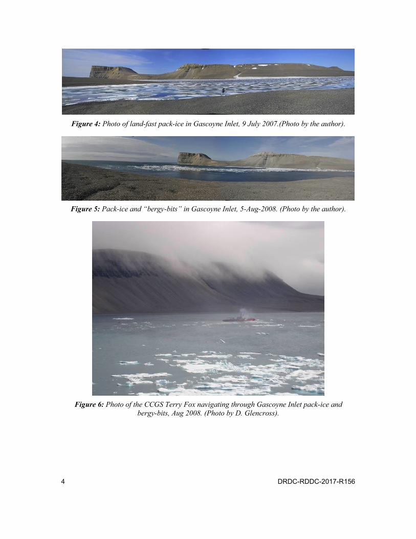
Figure 4: Photo of land-fast pack-ice in Gascoyne Inlet, 9 July 2007.(Photo by the author). . . . . . . . . . . . . . . . . . . . . . . . . . . . . . 4
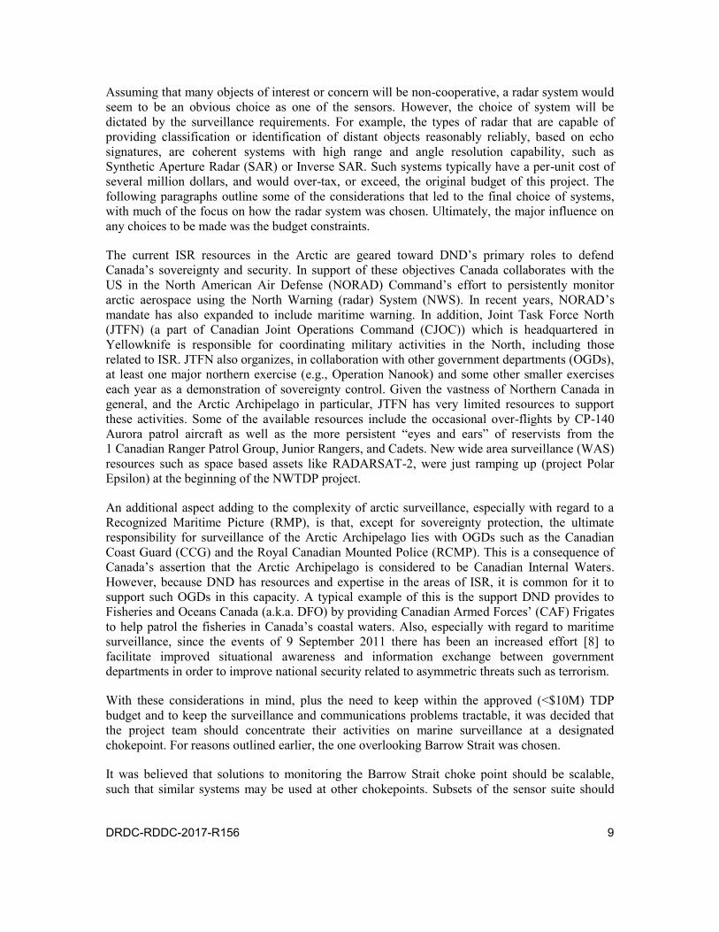
Figure 5: Pack-ice and “bergy-bits” in Gascoyne Inlet, 5-Aug-2008. (Photo by the author). . . . . . . . . . . . . . . . . . . . . . . . . . . . . . 4
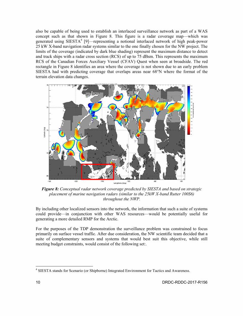
Figure 6: Photo of the CCGS Terry Fox navigating through Gascoyne Inlet pack-ice and bergy-bits, Aug 2008. (Photo by D. Glencross). . . . . . . . . . . . . . 4
Figure 7: Photo of a large 40 m tall grounded iceberg (foreground) and ~12 m tall 2 km by 6 km ice-island (background) near the mouth of Gascoyne Inlet, 4-Aug.-2012. (Photo by the author). . . . . . . . . . . . . . . . . . . . . . 5
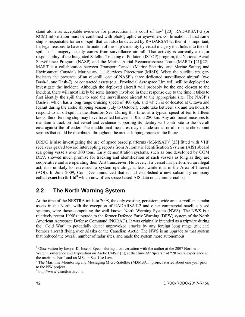
Figure 8: Conceptual radar network coverage predicted by SIESTA and based on strategic placement of marine navigation radars (similar to the 25kW X-band Rutter 100S6) throughout the NWP. . . . . . . . . . . . . . . . . . 10
Figure 9: Nominal NWS radar coverage map of Canada and Alaska. Red is associated with the FPS-117 long range radars, and the blue is associated with the FPS-124 short range (gap filler) radars. The “push-pin” icons represent former DEW line sites no longer a part of the NWS. (Sites and geographic locations obtained from [24]). . . . . . . . . . . . . . . . . . . . . . . . . 13
Figure 10: Potential marine surveillance coverage (red circles) that might be provided by appropriate modification of selected NWS radar systems. This potential coverage can be compared to merchant shipping traffic (upper right) reported during 1 July–31 Oct 2003. . . . . . . . . . . . . . . . . . . . . . 14
Figure 11: Empirical data showing effective RCS of various merchant ship sizes when viewed at low grazing angles with a marine navigation radar similar to the one used at NESTRA [35][36]. . . . . . . . . . . . . . . . . . . . . . 18
Figure 12: SIESTA range and coverage predictions for a 25kW X-band radar placed on top of Cape Liddon at 74.62861°N, 91.168333°W at an altitude of 320 m ASL. The green dots show the approximate maximum range to detect the vessels on the right, for their average RCS. . . . . . . . . . . . . . . . . . . . 18
x DRDC-RDDC-2017-R156
Figure 13: (from [56]) RCS profile [58][60] for a full-scale B-26 Marauder two-engine medium-bomber aircraft at a radar frequency of 3 GHz as a function of azimuth angle. The photos to the right compare the B-26 with a similar sized, but smaller DHC-6 Twin Otter. . . . . . . . . . . . . . . . . . . . 20
Figure 14: (from [56]) Low flying aircraft geometry with respect to a Rutter 100S6 radar on Cape Liddon. . . . . . . . . . . . . . . . . . . . . . . . . . 21
Figure 15: Canadian Forces Auxiliary Vessel (CFAV) Quest, used as a platform for experiments with ship based sensors for operational vessels (such as frigates and destroyers) and acting as a cooperative “target.” . . . . . . . . . . . 27
Figure 16: Theoretical azimuthal radar cross section profile of the CFAV Quest at a range of 20 km for a grazing angle of 0.1; the dashed circle represents the overall mean RCS. The prediction compares favourably with actual experimental observations [64]. . . . . . . . . . . . . . . . . . . . . . . . . . 27
Figure 17: Broadside RCS estimates for the Quest as a function of grazing angle; the blue curve is for the starboard side facing the radar and the red curve is for the port side. The graph on the right is an expanded view of the graph on the left for a grazing angle of 0 to 1°. . . . . . . . . . . . . . . . . . . . . . . 28
Figure 18: End-on RCS estimates for the Quest as a function of grazing angle; the blue curve is for the bow facing the radar and the red curve is for the stern. The graph on the right is an expanded view of the graph on the left for a grazing angle of 0 to 1°. . . . . . . . . . . . . . . . . . . . . . . . . . . 28
Figure 19: Area around Halifax Harbour showing the location of Osborne Head (inset upper left) and NESTRA (inset upper right); the NESTRA photo also shows the relative locations of the Radar/RWR truck and the CANDISS truck indicated by white rectangles. . . . . . . . . . . . . . . . . . . . . 31
Figure 20: Panoramic photos of the NESTRA site overlooking the Atlantic during a calm day in Oct. 2008 prior to the Trials. The pictures were taken at roughly the same location as the DRDC Valcartier van for CANDISS. . . . . . . . . 32
Figure 21: One view of the Radar/RWR truck showing the set-up of the RWR, Radar and communications antennas. The photo was taken on the relatively calm Tues. morning of Dec. 9 after the previous night’s storm. . . . . . . . . . . . 33
Figure 22: A view of relative set-up for all of the AW sensors at NESTRA (excluding AIS) on the morning of Tues. 9 Dec (photo by the author). . . . . . . . . 33
Figure 23: External photo of the Radar/RWR truck during the tail end of one of the early morning runs (12 am to 12 noon) on Wednesday, 10-Dec; notice the shimmed metal stabilizer (two on the opposite side) used to suppress truck rocking and vibration due to wind action. The inset shows how the Radar/RWR truck was configured for the trials. . . . . . . . . . . . . . . . . . . . . . . 34
Figure 24: Inside the rental truck used to house the Radar/RWR processors and personnel (photos taken by the author on the morning of 9 Dec. 2008). . . . . . . . . 35
Figure 25: Connections for the watts up?PRO power meter. . . . . . . . . . . . . 35

DRDC-RDDC-2017-R156 xi
Figure 26: Duplicate of the trihedral corner reflector used on the RHIB for radar calibration purposes. . . . . . . . . . . . . . . . . . . . . . . . . 37
Figure 27: Theoretical RCS profiles of a 0.7 m triangular trihedral corner reflector at 9.41GHz for incidence angles, , of 90 (red), 80, 70, 60, 50, and 40 and horizontally polarized on transmit and receive. . . . . . . . . . . . . . 38
Figure 28: Theoretical RCS profiles of a 0.7 m triangular trihedral corner reflector at 9.41GHz for incidence angles,, of 90 (red), 100, 110, 120, 130, and 140 and horizontally polarized on transmit and receive. . . . . . . . . . . . 38
Figure 29: Theoretical RCS profiles of a 0.7 m triangular trihedral corner reflector at 9.41GHz for incidence angles, , of 90 (red), 800, 70, 60, 50, and 40 and vertically polarized on transmit and receive. . . . . . . . . . . . . . . 39
Figure 30: Theoretical RCS profiles of a 0.7 m triangular trihedral corner reflector at 9.41GHz for incidence angles,, of 90 (red), 100, 110, 120, 130, and 140 and vertically polarized on transmit and receive. . . . . . . . . . . . . 39
Figure 31: Triangular Trihedral Corner Reflector geometry associated with the previous four figures. The maximum RCS value occurs along the axis of symmetry where =90 . . . . . . . . . . . . . . . . . . . . . . . . . . . 40
Figure 32: Measured RCS patterns (left) from a triangular corner reflector; note that the maximum RCS for this corner reflector’s measurements should be only 34.4 dBsm according to Equation (3). The above figures are from Skolnik [66] but originated by Robertson [67]. . . . . . . . . . . . . . . . . . . . . 41
Figure 33: SIESTA radar coverage predictions plots (minimum detectable RCS) for NESTRA based on an antenna at an altitude of 27 m ASL and assuming a distributed target height of up to 20 m ASL. . . . . . . . . . . . . . . 43
Figure 34: Predicted radar coverage for a 27 m ASL antenna and a point target of 2 m ASL, at SS1 with no precipitation. The plot to the left is a corresponding slice along a bearing radial of 140. . . . . . . . . . . . . . . . . . . . . 44
Figure 35: Predicted radar coverage as in Figure 34 but assuming a distributed target (not a point source) up to 2 m ASL. The predicted maximum range to detect a small vessel of 10 to 15 dBsm is 14 to 16 km. The maximum detectable range of a 75 dBsm target is 31.4 km. . . . . . . . . . . . . . . . . . . . . . 44
Figure 36: Predicted radar coverage as in Figures 34 and 35 except that it was generated assuming a distributed target up to 2 m above the surface, a Sea State of 4, and a precipitation rate of 1 mm/hr. The maximum detection range for a 75 dBsm target is 28.2 km. . . . . . . . . . . . . . . . . . . . . . . . . . 45
Figure 37: Predicted radar coverage as in Figures 34 to 36 except that it was generated assuming a distributed target up to 20 m above the surface, a Sea State of 4, and a precipitation rate of 1 mm/hr. The maximum detection range for a target of 75 dBsm is predicted to be 42.7 km. . . . . . . . . . . . . . . . . 45
Figure 38: Locations of six weather stations (indicated by cloud/rain symbols), in and around Halifax, that contribute to Environment Canada’s archival database. . 47

xii DRDC-RDDC-2017-R156
Figure 39: Temperature variation recorded at Osborne Head DND from 7–12 Dec. 2008. 48
Figure 40: Wind Speed profile recorded at Osborne Head DND from 7–12 Dec. 2008. The green shaded areas represent the times during which radar data was collected. . . . . . . . . . . . . . . . . . . . . . . . . . . . . 48
Figure 41: Stitched panorama from pictures taken at 7:55 am Monday morning at NESTRA. . . . . . . . . . . . . . . . . . . . . . . . . . . . . 50
Figure 42: High surf directly east of Osborne Head (NESTRA) at approximately 8:00 am on Monday morning (photo by the author). . . . . . . . . . . . . . . . 50
Figure 43: Photos by the author showing the wind-blown surf just east of NESTRA (top left) and about 3 km south of NESTRA (top right, and bottom), just east of Hartlen Point. These can be compared to the photos in Figure 20. . . . . . . 50
Figure 44: View looking east from NESTRA at 1:18 pm on Monday showing the surf due to the high winds; the CFAV Quest can also be seen in the centre of the photo with an expanded view shown in the inset (photo by the author). . . . . . . 51
Figure 45: Photo of the AWS with the main NESTRA building in the background; taken at 4:21 pm Monday afternoon (courtesy of Dr. V. Larochelle). . . . . . . . 51
Figure 46: RHIB approaching the Quest after the calibration run on Tuesday afternoon, 9 Dec. 2008. . . . . . . . . . . . . . . . . . . . . . . . . . . . . 52
Figure 47: Photo taken by the author looking eastward from NESTRA on Tuesday morning, 9 Dec. 2008. The inset is a blow-up of the CFAV Quest (on the left) and a freighter (Atlantic Superior) heading to Halifax Harbour.. . . . . . . 52
Figure 48: Photo by the author taken on the calmest day of the trials, Tues. 9 Dec. 2008. The inset shows the Quest and a smaller fishing vessel to its right. . . . . . 53
Figure 49: Photo by the author taken at 11:23 local time, Tues. 9 Dec. 2008. The inset on the right shows a blow-up of the Quest, and the one on the left shows a couple of the local fishing vessels. . . . . . . . . . . . . . . . . . . . . . 53
Figure 50: Surf east of Osborne Head, about 200 m from the radar site, on Thursday afternoon around 1:30 pm. Notice that all of the snow has melted by this point. (Photo by the author). . . . . . . . . . . . . . . . . . . . . . . . 54
Figure 51: Photo taken by the author from NESTRA on Thursday afternoon 11, Dec. 2008, showing the weather conditions on the last day of data collection. The inset shows one of the small craft used by local lobster fishermen. . . . . . 54
Figure 52: Valcartier AIS tracks; the legend displays the MMSI number associated with each ship track during the period from 13:09 to 17:35 on Monday Dec. 8. . . 57
Figure 53: Valcartier AIS tracks; the legend displays the MMSI number associated with each ship track during the period from 17:35 on Dec. 8 to 08:57 Dec. 9. . . . 58
Figure 54: Valcartier AIS tracks including Quest with manoeuvres; the legend displays the MMSI number associated with each ship track during the period from 08:57 to 14:44 on Dec. 9. . . . . . . . . . . . . . . . . . . . . . . 59

DRDC-RDDC-2017-R156 xiii
Figure 55: Valcartier AIS tracks; the legend displays the MMSI number associated with each ship track during the period from 14:44 on Dec. 9 to 01:41 on Dec. 10. . 60
Figure 56: Valcartier AIS tracks; the legend displays the MMSI number associated with each ship track during the period from 01:41 to 09:38 on Dec. 10. . . . . . 60
Figure 57: AIS tracks; the legend displays the MMSI number associated with each ship track during the period from 09:39 on Dec. 10 to 02:01 on Dec. 11. . . . . . 61
Figure 58: AIS tracks; the legend displays the MMSI number associated with each ship track during the period from 02:01 to 04:42 on Dec. 11. . . . . . . . . . 62
Figure 59: AIS tracks for the period from 04:42 to 07:50 on Dec. 11; the legend displays the MMSI number associated with each ship track. . . . . . . . . . . . 63
Figure 60: AIS tracks for the period from 07:50 to 09:15 on Dec. 11; the legend displays the MMSI number associated with each ship track. . . . . . . . . . . . 63
Figure 61: AIS tracks for the period from 09:15 to 10:32 on Dec. 11; the legend displays the MMSI number associated with each ship track. . . . . . . . . . . . 64
Figure 62: AIS tracks for the period from 10:32 to 12:51 on Dec. 11; the legend displays the MMSI number associated with each ship track. . . . . . . . . . . . 65
Figure 63: AIS tracks for the period from 12:51 to 16:00 on Dec. 11; the legend displays the MMSI number associated with each ship’s track. . . . . . . . . . . . 66
Figure 64: Photo of the Antwerp Express container ship; from [68]. . . . . . . . . . 69
Figure 65: Sir William Alexander, Canadian Coast Guard Ship (CCGS) ice-breaker; from [69]. . . . . . . . . . . . . . . . . . . . . . . . . . . . . . . 70
Figure 66: Photographs of the CCGS Louis St. Laurent from the CCG web-site [69]. . . 70
Figure 67: Photos of Skandi Bergen; from [70]. . . . . . . . . . . . . . . . . . 70
Figure 68: Photos of the cargo ship Rega; from [71]. . . . . . . . . . . . . . . . 71
Figure 69: Photos of the container ship Undine; from [72]. . . . . . . . . . . . . . 71
Figure 70: Photo of the Atlantic Bear tugboat, from an Atlantic Towing Ltd brochure [73]. . . . . . . . . . . . . . . . . . . . . . . . . . . . . . . 71
Figure 71: Photos of the OOCL San Francisco, container ship; from [74]. . . . . . . . 72
Figure 72: Photos of the cargo/container ship Sirius Highway; from [75]. . . . . . . . 72
Figure 73: Photo of the container ship Atlantic Concert; (photo by the author, 20 Oct. 2005). . . . . . . . . . . . . . . . . . . . . . . . . . . . . . . 72
Figure 74: Photos of the container ship Zim Pusan; from [76] (Photo by K. Watson). . . 73
Figure 75: Photographs of the cargo ship British Courtesy; from [77] (Left photo by D. Kannengießer). . . . . . . . . . . . . . . . . . . . . . . . . . . 73
Figure 76: Photos of the tanker ship Maria Desgagnes; from [78]. . . . . . . . . . . 73
Figure 77: Photo of the container ship Atlantic Superior; from [79] (Photo by K. Watson). 74
xiv DRDC-RDDC-2017-R156
Figure 78: A photograph of the Nirint Force, a container vessel in the Halifax area during the NESTRA Trials; from [80] (Photo by M. Schindler). . . . . . . . . . 74
Figure 79: Photograph of the tug Svitzer Bedford (Photo by M. MacKay [81]). . . . . . 74
Figure 80: Photo of the crude-oil shuttle tanker Kometik; image from “Capnkens Blog” [82]. . . . . . . . . . . . . . . . . . . . . . . . . . . . . . . 75
Figure 81: Photo (by M. MacKay [83]) of the tug Atlantic Oak (very similar to Atlantic Bear). . . . . . . . . . . . . . . . . . . . . . . . . . . . . . . 75
Figure 82: SeaScan Server software GUI to select a default data file for raw data collection or playback prior to starting the data logging using SeaView. . . . 77
Figure 83: This chart shows the approach to Halifax harbour, including four stationary buoys that were detected by the radar system and used to help calibrate its pointing direction. The blue circles represent the recorded positions of the buoys [85][86], and the purple flags represent their respective radar tracks. . . 79
Figure 84: The maximum detection range for the pilot-boat APA No. 1 was 12.0 km, observed at around 11:06 am Dec. 10 while the conditions were SS 3 to 4 with cloudy conditions but very little precipitation. (Note: the picture of APA 1 on the right, courtesy of Tim Hammond of DRDC – Atlantic Research Centre, was taken during different set of trials.) . . . . . . . . . . . . . . . . 80
Figure 85: Chart (upper left) showing plotted radar tracks for a number of fishing vessels (black ellipses), four tethered marker buoys (red flags), and a number of larger vessels including the Quest (coloured polygons).The fishing/lobster boats were detected to a range of over 10 km. Photos of typical vessels seen in the area under day and night conditions (extracted from CANDISS video from the trials) are shown around the periphery. . . . . . . . . . . . . . . . . 81
Figure 86: SeaView radar display (medium range mode) of mostly small boats in the NESTRA area. The display n the upper left is with the track display on while the upper right is with it off, and the lower image is an expanded view. . . . 82
Figure 87: SeaView Radar track (MR mode) of the RHIB from 15:12:45 to 15:26:25 on 9 December 2008. The RHIB remained on station (5.23 nmi from NESTRA at bearing 115T) until approximately 15:20 before returning to the Quest. . . . 83
Figure 88: SeaView radar display during a slightly earlier RHIB recording (track 202) at about 15:06; like Figure 87 but with a 0 min. “Target Trail Length” resulting in a much cleaner view. . . . . . . . . . . . . . . . . . . . . . . 84
Figure 89: Radar (blue) and GPS (red) tracks for the RHIB; the white ellipses represent the radar track for the Quest. There was a slight bearing (0.22) and range offset (~80 m) between the radar and GPS locations, as well as a slight displacement in time (<3min.). The series of plots are gradually zoomed in to show the most detail in the lower right. . . . . . . . . . . . . . . . . 85
Figure 90: The last contact range for the CFAV Quest in this run (taken on Dec. 11 at 4:50 am AST, Halifax time) was 28.6 km. This is consistent with SIESTA predictions for SS 3 and rain rate of about 1 mm/hr for a stern RCS of between 40 and 65 dBsm. . . . . . . . . . . . . . . . . . . . . . . . . . 86

DRDC-RDDC-2017-R156 xv
Figure 91: Rutter 100S6 SeaView PPI display with an expanded portion from showing the CFAV Quest radar track (#19) which also plotted in Figure 90. . . . . . 87
Figure 92: Radar (light & dark blue ellipses) and AIS (black dots) tracks for the CFAV Quest on the morning of 11-Dec. 2008. The inset in the lower left is an expanded view of vessel manoeuvre showing how well the radar tracked the ship during a complex manoeuvre with a turn radius of less than 120 m. . . . 88
Figure 93: Tight turn of radius 150 m executed by the CFAV Quest, captured by both the AIS (light blue triangles) and the radar (purple and white). The purple and white markers are respectively before and after slight corrections were made to the radar range and bearing estimates. The centre of the circle is at 14.5 km from NESTRA. . . . . . . . . . . . . . . . . . . . . . . . . . . 89
Figure 94: More radar (white ellipses) and AIS (red) tracks for the Quest from the morning of 11-Dec. The radar began tracking the ship at around 25 km when the Sea-State was between 2 and 3 with a rain rate of about 1 mm/hr. . . . . 89
Figure 95: AIS (green) and Radar (red) tracks for the Algoscotia on the morning of 11-Dec. The Sea State was 2 to 3 and rain rate was roughly 1 mm/hr. The maximum detection range of 28.2 km is consistent with a vessel of this size and aspect with respect to the radar-to-target geometry. The photos of the Algoscotia on the right are courtesy of Tim Hammond. . . . . . . . . . . 90
Figure 96: PPI display from SeaView for the inbound Algoscotia plotted in Figure 95. . . 90
Figure 97: Radar+AIS tracks of two large container ships, the inbound OOCL San Francisco (two photos, upper right) and outbound Zim Pusan (two photos, lower right). The first was detected at 9:49 am Dec. 10 at 33.6 km; the latter at 10:02 am the same day at a range of 35 km. The conditions were SS 1 to 2 with no precipitation. (Photos courtesy of Tim Hammond). . . . . . . . . 91
Figure 98: Radar+AIS tracks of the outbound OOCL San Francisco on Thursday morning, 11-Dec. 2008 with SS 2-3 and a rain rate of 1–2 mm/hr. The maximum detection range of the ship is consistent with its size (stern approx. 26 m ASL) and the SIESTA predictions in Figure 37. . . . . . . . . . . 92
Figure 99: Track (green) of an aircraft bisecting the red automatic target acquisition zone, the apparent heading to Shearwater AFB at about 110 knots. Although the radar could easily detect the target, the tracker had difficulty maintaining the track. Each range ring is spaced by 3 Nm. . . . . . . . . . . . . . . . 93
Figure 100: Track of an aircraft/helicopter (MR mode) heading toward Shearwater AFB. The target course is outlined with a white polygon to highlight the radar tracks, and where the radar lost track as the aircraft made a sharp manoeuvre around the CFAV Quest (yellow dot at the bend). Each range ring is spaced 3nmi (5.6 km). . . . . . . . . . . . . . . . . . . . . . . . . . . . . . . 93
Figure 101: Series of radar plots showing the progress of an aircraft (highlighted in each image by a white circle centred on the aircraft echo) of unknown type. The series of plots is used to show the aircraft location because the tracker had a problem locking on due to fades and land clutter interference. The sequence of plots is ordered by the number shown in the upper right corner of each display. 94
xvi DRDC-RDDC-2017-R156
Figure 102: Screen capture from the WUP GUI display showing the power consumption of the 100S6 radar over a period of 2 h on 10-Dec.-2008. The plot shows the radar’s average power consumption while rotating at 45 rpm, during relatively high wind conditions as well as when the transmitter and antenna drive were turned off and the surge on initial turn on. . . . . . . . . . . . . . . . 95
Figure 103: Screen captures showing the 100S6 radar control and display GUI when the “Pulse Filter” option was turned off (left), and then on (right) over the same period (9 Dec. 2008, 14:28:02). The red oval in the upper left of each disp lay shows the location and status of the control “button.” Most of the “false” plots on the left align with two green bearing lines (135 and 184) that also coincide with the bearings of ships presumably with similar X-band navigation radars. . . . . . . . . . . . . . . . . . . . . . . . . . . . . . 97
Figure 104: Screen captures from the 100S6 radar control and display GUI when the “Pulse Filter” option was turned off (left), and when it was turned on (right) during the same period (9 Dec. 2008, 14:29:44). The left bearing line aligned with the unfiltered contacts in the image to the left has moved to 187, corresponding to a single target, whereas the right bearing line appears stationary, possibly due to two targets going in opposite directions. . . . . . 98
Figure 105: Screen captures from the 100S6 radar control and display GUI when the “Pulse Filter” option was turned off (left), and when it was turned on (right) during the same period (9 Dec. 2008, 14:32:37). As the target ship on the right changes bearing (e.g.,185 to 190), the “false” plots accumulate over the sector swept out by the bearing line. . . . . . . . . . . . . . . . . . 99
Figure 106: Relative geometry for estimating the synchronization constraints between the local and target radar antennas to use the local radar as an RWR. . . . . . 101
Figure A.1: Run A (outbound: RED; inbound: BROWN). The GREEN circle and BLUE lines defines the laser radiation zone. . . . . . . . . . . . . . . . . 113
Figure A.2: Run B (outbound: RED; inbound: BROWN). The GREEN circle and BLUE lines defines the laser radiation zone. . . . . . . . . . . . . . . . . 114
Figure B.1: Rutter 100S6 radar network architecture. . . . . . . . . . . . . . . 117
Figure B.2: The photo on the left shows the Rutter radar at a temporary testing location at DRDC – Ottawa Research Centre. The photo on the right shows the 16 ft tower that the radar will be mounted on in the Arctic, as it was being test-installed at DRDC; the tower was not available for NESTRA. . . . . 119
Figure D.1: CCGS Louis St. Laurent. . . . . . . . . . . . . . . . . . . . . . 130
Figure D.2: CCGS Henry Larsen. . . . . . . . . . . . . . . . . . . . . . . 130
Figure D.3: CCGS Des Groseilliers. . . . . . . . . . . . . . . . . . . . . . 130
Figure D.4: CCGS Amundsen. . . . . . . . . . . . . . . . . . . . . . . . . 131
Figure D.5: CCGS Terry Fox. . . . . . . . . . . . . . . . . . . . . . . . . 131
Figure D.6: CCGS Sir Wilfred Laurier. . . . . . . . . . . . . . . . . . . . . 131
Figure D.7: Akademik Ioffe. . . . . . . . . . . . . . . . . . . . . . . . . 131
DRDC-RDDC-2017-R156 xvii
Figure D.8: (M/V) Explorer. Note that this ship actually sank in the Antarctic in 2008, but that doesn’t preclude cruise ships of similar size transiting the Arctic in the future. . . . . . . . . . . . . . . . . . . . . . . . . . . . . 132
Figure D.9: Kapitan Khlebnikov. . . . . . . . . . . . . . . . . . . . . . . . 132
Figure D.10: Alexander Von Humboldt. . . . . . . . . . . . . . . . . . . . . 132
Figure D.11: Hanseatic. . . . . . . . . . . . . . . . . . . . . . . . . . . . 132
Figure D.12: M/V Bremen. . . . . . . . . . . . . . . . . . . . . . . . . . 133
Figure D.13: National Geographic Explorer. . . . . . . . . . . . . . . . . . . . 133
Figure D.14: Prince Albert II.. . . . . . . . . . . . . . . . . . . . . . . . . 133
Figure D.15: Ocean Nova. . . . . . . . . . . . . . . . . . . . . . . . . . . 133
Figure D.16: Lyubov Orlova and sister ship Clipper Adventurer. . . . . . . . . . . 133
Figure D.17: Akademik Sholkaskiy. . . . . . . . . . . . . . . . . . . . . . . 134
Figure D.18: R/V Xuelong. . . . . . . . . . . . . . . . . . . . . . . . . . 134
Figure D.19: Amazon Express. . . . . . . . . . . . . . . . . . . . . . . . . 134
Figure D.20: Oden. . . . . . . . . . . . . . . . . . . . . . . . . . . . . . 134
Figure D.21: Aliacmon River. . . . . . . . . . . . . . . . . . . . . . . . . 135
Figure D.22: Algosoo. . . . . . . . . . . . . . . . . . . . . . . . . . . . 135
Figure D.23: Anna Desgagnés. . . . . . . . . . . . . . . . . . . . . . . . . 135
Figure D.24: Brouwersgracht/Scheldegracht. . . . . . . . . . . . . . . . . . . 135
Figure D.25: Ken Ryn. . . . . . . . . . . . . . . . . . . . . . . . . . . . 135
Figure D.26: Camilla Desgagnés. . . . . . . . . . . . . . . . . . . . . . . . 135
Figure D.27: (M/T) Tellus. . . . . . . . . . . . . . . . . . . . . . . . . . . 136
Figure D.28: Umiavut. . . . . . . . . . . . . . . . . . . . . . . . . . . . 136
Figure D.29: M/V Astron. . . . . . . . . . . . . . . . . . . . . . . . . . . 136
Figure D.30: Alex Gordon. . . . . . . . . . . . . . . . . . . . . . . . . . . 136
Figure D.31: Edgar Kotokak. . . . . . . . . . . . . . . . . . . . . . . . . . 136
Figure D.32: M/V Keewatin. . . . . . . . . . . . . . . . . . . . . . . . . . 136
Figure D.33: Atlantic Teak. . . . . . . . . . . . . . . . . . . . . . . . . . 137
Figure D.34: Kelly Ovayuak. . . . . . . . . . . . . . . . . . . . . . . . . . 137
Figure D.35: Eastern Tugger. . . . . . . . . . . . . . . . . . . . . . . . . . 137
Figure D.36: Arctic Endurance. . . . . . . . . . . . . . . . . . . . . . . . . 137
Figure D.37: R/V Knorr.. . . . . . . . . . . . . . . . . . . . . . . . . . . 138
Figure D.38: R/V Geolog Dmitri. . . . . . . . . . . . . . . . . . . . . . . . 138
xviii DRDC-RDDC-2017-R156
Figure D.39: Bin Hai 517. . . . . . . . . . . . . . . . . . . . . . . . . . . 138
Figure D.40: R/V Strait Signet. . . . . . . . . . . . . . . . . . . . . . . . . 138
Figure D.41: Aurora Magnetica. . . . . . . . . . . . . . . . . . . . . . . . 138
Figure D.42: Baloum Gwen. . . . . . . . . . . . . . . . . . . . . . . . . . 138
Figure D.43: R/V White Holly. . . . . . . . . . . . . . . . . . . . . . . . . 139
Figure D.44: Arctic Wanderer. . . . . . . . . . . . . . . . . . . . . . . . . 139
Figure D.45: Southern Star. . . . . . . . . . . . . . . . . . . . . . . . . . 139
Figure D.46: Geraldine. . . . . . . . . . . . . . . . . . . . . . . . . . . . 139
Figure E.1: Schooner sailboat. . . . . . . . . . . . . . . . . . . . . . . . . 141
Figure E.2: Royal Lowell lobster boat. . . . . . . . . . . . . . . . . . . . . 141
Figure E.3: Stanley Greenwood lobster boat . . . . . . . . . . . . . . . . . . 141
Figure E.4: Atkinson lobster boat. . . . . . . . . . . . . . . . . . . . . . . 141
Figure E.5: Multipurpose fishing boat. . . . . . . . . . . . . . . . . . . . . 141
Figure E.6: Scallop boat (ex Marine Patrol Boat). . . . . . . . . . . . . . . . . 141
DRDC-RDDC-2017-R156 xix
List of Tables
Table 1: RCS for point like targets [2]. . . . . . . . . . . . . . . . . . . . . 7
Table 2: Empirical Ship RCS estimates related to ship size and type [35]. . . . . . . 17
Table 3: Chart comparing a Kenn Borek Airlines Twin Otter DHC-6 [57] to a B-26 Marauder [59]. . . . . . . . . . . . . . . . . . . . . . . . . . . 21
Table 4: Cost/Endurance comparison for persistent surveillance platforms based on information up to 2007 [61][62]. . . . . . . . . . . . . . . . . . . . 23
Table 5: Some examples of solid state coherent airborne radar systems; the L-88 variants are usually on an aerostat whereas the SeaSpray variants have been used in aerostats, fixed and rotary wing manned aircraft, and UAVs (e.g., Predator). . . . . . . . . . . . . . . . . . . . . . . . . . . . . 24
Table 6: Weather Conditions at Osborne Head & Shearwater Airport for Monday 7-Dec. through Thursday 11-Dec 2008. . . . . . . . . . . . . . . . . . 49
Table 7: Time periods and number of ships observed during each period associated with each set of AIS tracks in Figure 52 to Figure 63. . . . . . . . . . . . . 55
Table 8: List of ships tracked by AIS in the NESTRA AOI during the AWS trials; the dimensions of each ship—identified by MMSI#, call-sign, and ship’s name—are provided, along with their gross tonnage and, where possible, their RCS estimates based on Equation (2). . . . . . . . . . . . . . . . . . . . 67
Table 9: Radar detection ranges—both observed and predicted by SIESTA for three environmental cases—for ships listed in Table 8. . . . . . . . . . . . . 68
Table 10: Marine Buoys in the Approach to Halifax harbour; the values in parenthesis represent the averaged “tracked” positions from the radar data. . . . . . . . 78
Table B.1: Radar system description. . . . . . . . . . . . . . . . . . . . . . 118
Table B.2: Mechanical dimensions. . . . . . . . . . . . . . . . . . . . . . 118
Table C.1: NESTRA Trials radar data files and notes. . . . . . . . . . . . . . . 120
Table D.1: Listing of vessels observed to operate in arctic waters during the period 2003 to 2008 obtained from DND’s “Global Position Warehouse;” also included are their respective sizes, RCS estimates, the sources of the ship’s information, and any associated pictures. . . . . . . . . . . . . . . . . . . . . 124
Table E.1: Listing of typical small vessel types (lobster, fishing, etc.) that might be expected in the NESTRA AOI along with any available size or construction information, the sources of the information, and associated photographs. . . 140

xx DRDC-RDDC-2017-R156
Acknowledgements
The author would like to thank the following people for their valuable assistance:
Mr. Ed Riseborough for his help with analysis of the radar data; his MATLAB software for extracting and recording the target track data from the radar system manufacturer’s SeaTrack tracking program was invaluable;
Dr. Silvester Wong, for his help generating the RCS profiles for the triangular trihedral corner reflector shown in Figures 27 to 30;
Dr. Luc Forand and Dr. Vincent Larochelle of DRDC Valcartier, for the photos and CANDISS video data they provided as well as the AIS and GPS data they provided for use as ground-truth for the radar detections and tracks;
Mr Denis Lamothe, for his valuable technical and logistical assistance during the deployment and performance of the radar portion of the trials;
Mr Nathan Kashyap, for his assistance in extracting the arctic ship traffic information from the Global Position Warehouse database; and
Dr Tim Hammond, who provided photographs for several of the ships, which he had acquired using DRDC Atlantic’s Automated Ship Image Acquisition (ASIA) system located near the entrance to Halifax Harbour.
DRDC-RDDC-2017-R156 1
1 Introduction
In August of 2008 the Northern Watch (NW) project, as part of the Technology Demonstration Program, attempted to perform some initial early-phase sensor evaluation and integration field trials at Gascoyne Inlet/Cape Liddon, on the southwest corner of Devon Island, and overlooking a maritime chokepoint through Barrow Strait. The location of these trials is shown in Figure 1 and Figure 2. As pointed out in an earlier report by the author [1], severe weather effects presented logistical challenges that proved to be insurmountable at the time, and only a minimal portion of the trials objectives were accomplished. While some data were recorded by the Automatic Dependent Surveillance-Broadcast (ADS-B) receiver and a radar-warning-receiver/direction-finder (RWR), developed in-house at DRDC, neither the radar system, nor the camera imaging system (Canadian Arctic Night and Day Imaging Sensor System, CANDISS) could be deployed. A brief, but more detailed summary of the purpose and outcomes of those trials is provided in [1].
Figure 1: Potential arctic trials sites for the NWTDP: the project’s main base-camp and
(back-end) processing site for the UW sensors at Gascoyne Inlet (red X, upper right); and AW sensors location and proposed processing site on top of Cape Liddon (lower right).

2 DRDC-RDDC-2017-R156
Figure 2: An aerial perspective of the arctic trials sites based on a photo taken in 2008 by
Mr. Nelson McCoy.1 Radstock Bay, and Gascoyne Inlet were coloured light blue in order to provide a higher land-sea contrast; sea ice is visible in the foreground.
Since the original NW test and development schedule was so tightly constrained by the preparation required for each year’s planned Arctic field trials (i.e., originally once per summer for three years), the NW Science Team decided it needed to quickly organize a coordinated Above Water Sensors (AWS) field trial somewhere in the South. This would allow them to perform some of the testing that was initially scheduled for the Arctic, and where logistical concerns could be more easily addressed. The site that was chosen was the Naval Electronic Systems Test Range Atlantic (NESTRA). The NESTRA site was chosen for the following reasons:
1. Because it met all of the power, accommodations, accessibility, availability, safety and cost requirements specified in [1];
2. A cooperative target (i.e., CFAV Quest) could be procured within a short lead time;
3. There would be a large number of targets of opportunity available because of the proximity to a major port and shipping lanes; and
1 Mr. McCoy was the Deputy Project Manager and Trials Coordinator at the time of the first Arctic Trials in August 2008.
DRDC-RDDC-2017-R156 3
4. The short lead time meant that trials could be performed in Halifax in early December when weather conditions might be expected to be very similar to typical Arctic conditions that might be seen in the July-August period.
Despite the positive aspects of performing the trials at NESTRA, there were some also drawbacks, some of which are listed as follows:
1. Since the site is only about 30 m above sea level (ASL), including sensor platforms or towers, it did not meet the highly desired condition of altitude over 100 m to provide the sensor(s) with a long line-of-sight (LOS);
2. Radar propagation in December, in the Halifax region, could be sufficiently different from conditions anticipated in the Arctic for the following reasons:
a. The air-sea temperature difference east of the Halifax harbour is expected to be significantly different than what might be expected in Barrow Strait because of the influence of the Gulf Stream along the east coast;
b. There is very little sea-ice in and around the Halifax harbour in early December, whereas in the vicinity of Gascoyne Inlet, in early August, there can often be significant remnants of ice flows moving back and forth through Lancaster Sound and Barrow Strait; there have also been numerous sightings of icebergs of varying sizes observed in the area. These conditions can lead to significant radar clutter problems (false alarms) caused by low level sea-ice, as well as shadowing effects caused by icebergs and ice-islands. Examples of both types of conditions are highlighted in Figure 3 to Figure 7 which show pictures taken by the author in 2007, 2008, and later in 2012.
However, the advantages of the NESTRA site were believed to far outweigh the drawbacks, at least for the first phase of the sensor evaluations.
Figure 3: Aerial view from the Twin Otter of pack-ice in Barrow Strait west of Gascoyne Inlet
(left, by the author) and at Gascoyne Inlet (right, by J. Lee), July 2007.
4 DRDC-RDDC-2017-R156
Figure 4: Photo of land-fast pack-ice in Gascoyne Inlet, 9 July 2007.(Photo by the author).
Figure 5: Pack-ice and “bergy-bits” in Gascoyne Inlet, 5-Aug-2008. (Photo by the author).
Figure 6: Photo of the CCGS Terry Fox navigating through Gascoyne Inlet pack-ice and
bergy-bits, Aug 2008. (Photo by D. Glencross).

DRDC-RDDC-2017-R156 5
Figure 7: Photo of a large 40 m tall grounded iceberg (foreground) and ~12 m tall 2 km by 6 km ice-island (background) near the mouth of Gascoyne Inlet, 4-Aug.-2012. (Photo by the author).
Although several years have elapsed between the time these trials first took place, and the completion of this report, it is felt that this report is nevertheless justified for the following reasons:
1. It provides a record of some of the initial project objectives, research objectives, and lessons-learned that guided subsequent NW decisions regarding research on sensor capabilities, sensor integration, and trials logistics, especially with regard to arctic applications;
2. The ground-truthed data sets acquired from the combined AWS systems constitute a database, mostly unclassified, that may be useful for researchers developing future sensor integration concepts;2
The purpose of this report is to describe the following itemized list, primarily from the radar perspective:
1. The rationale behind the choice of the Northern Watch sensors, with specific attention to the selection of the radar sensor (Section 2);
2. The scientific objectives of the NESTRA trials (Section 3);
3. The experimental equipment set-up (Section 4);
4. The expected performance of the radar at the NESTRA site as predicted by the radio frequency (RF) segment of the Scenario/Shipboard Integrated Environment System for Tactics and Awareness (SIESTA) (Section 5);
5. The environmental conditions encountered during the trials (Section 6);
2 Several Terabytes of radar (raw digitized), AIS, GPS and CANDISS datasets were provided to The Technical Cooperation Program (TTCP) Technical Panel-1 (TP-1) on Sensor Integration in 2010.

6 DRDC-RDDC-2017-R156
6. The initial analyses of the Rutter 100 S6 navigation radar detection and tracking capability as compared to ground truth provided by the ship self reports via Automatic Identification System (AIS) and Global Positioning System (GPS) (Section 7); and
7. The observations and conclusions given in Section 7.
This report also contains five annexes of supplementary information on the following:
1. Brief description of the different NESTRA Trial scenarios showing the planned waypoints and potential courses that would be followed by the CFAV Quest (Annex A);
2. A description of the Rutter 100S6 radar system (Annex B);
3. A listing of radar data files collected, along with associated trials notes (Annex C)
4. A listing and description of typical vessel traffic observed operating in arctic waters during 2003 to 2008 (Annex D); and
5. A listing and description of typical east coast fishing vessels that might have been observed by radar in the NESTRA area during the trials (Annex E).

DRDC-RDDC-2017-R156 7
2 Sensor Selection Rationale
In general, the sensor requirements for Arctic surveillance will strongly depend on the following considerations:
The targets of interest (size, speed, location (land, air or sea)); Table 1 [2] is a comparison chart of some typical radar cross section (RCS) values for targets of various physical sizes that nonetheless may look like point-like targets at X-band (8–12 GHz);
The desired persistence criteria such as time on target, update rate, etc.;
Sensor reliability (i.e., mean time before sensor system or platform failure);
Area of Interest (wide area vs. local surveillance);
System power requirements;
Degree of automation required;
The sensor operational environment (e.g., local climate characteristics, sensor mobility, and whether it is operating on land, sea, air or in space); and
Local infrastructure, including:
Shelter (including environmental control such as heating);
Power sources;
Communications to remotely access the sensor information and provide some measure of remote control plus system “health monitoring;” and
Proximity to communities or bases of operation to facilitate equipment maintenance.
Table 1: RCS for point like targets [2].
Targets RCS (m2) RCS (dBsm) Bird 0.01 -20 Man 1 0
Cabin cruiser 10 >10 Automobile 100 20
Truck 200 23 Corner reflector 203793 43.1
Following consultation with military sponsors, industry, and academia [3]–[7] and after due consideration by the project’s scientific team, the decision was made to scope the project’s main objective to be local surveillance of a maritime choke-point in the High Arctic on Barrow Strait. Some of the reasons behind this decision, and the subsequent selection of appropriate sensors will be provided in the rest of this section; special emphasis will be placed on the selection of the radar sensor.
3 At 9.41 GHz this would correspond to the maximum reflection from a trihedral corner reflector with a front edge about 1.6 m long or similarly at 3 GHz a TCR with a 2.84 m front edge.

8 DRDC-RDDC-2017-R156
With regard to the suitability of various radar systems and associated platforms to support surveillance of maritime vessel traffic in the High Arctic, the following list provides a few examples for consideration:
Conventional (low-cost, non-coherent) marine navigational radars (such as the Rutter 100S6 which was ultimately chosen for this project);
Airborne systems (patrol aircraft, aerostats, etc.) or similar systems converted for deployment to land based sites;
North Warning System radars such as the FPS-117 and FPS-124 modified for surface surveillance;
Satellite borne systems such as Synthetic Aperture Radar (domestic and foreign), e.g., RADARSAT 1 & 2, Envisat, TerraSAR-X, etc.; and
Over The Horizon (OTH) Radar, such as High Frequency Surface Wave Radar (HFSWR).
All such systems have associated strengths and weaknesses, not least of which is their overall cost of deployment and maintenance. Of the radar types mentioned, the focus of this report will be on the conventional, non-coherent, marine navigation radar. Due to its relatively low capital cost compared to more expensive coherent systems, this type of radar was chosen as one of the components of the choke-point surveillance suite that will be tested in the High Arctic as part of the Northern Watch TDP project. Some of the reasons for the selection of this system will be presented in the following paragraphs and sub-sections.
At the beginning of the NWTDP, there were few, if any, “officially” stated requirements for persistent arctic surveillance by DND, especially with regard to maritime surveillance. Until recently, most passages through the Arctic Archipelago were ice-bound and non-navigable for most of the year so shipping traffic was relatively low. These considerations, coupled with DND’s budget constraints, meant that maritime surveillance of the Arctic was low on DND’s list of priorities. However, with recent changes in climate, more shipping channels are opening and for longer periods of time. Now, increased interest in exploiting northern resources has led to a re-examination of the need for greater monitoring of, and presence in, the Arctic.
With this in mind, the NW project decided to examine the Intelligence, Surveillance and Reconnaissance (ISR) capabilities that were available in the Arctic, at that time, in order to identify potential cost-effective prototype solutions that might improve operational capabilities. The new capabilities to be demonstrated under this TDP had to fit within Canada’s “layered” defence concept—a combination of Wide Area Surveillance coupled with more localized resources. However, without stated requirements to use as guidelines, it was initially challenging to chart the course of the project with such an open ended problem statement.
For example, such requirements would normally identify the objects of interest (e.g., potential threats), the areas of concern, the level(s) of persistence, and the level(s) of detail (e.g., classification and/or identification) required. The requirements might also indicate the budget that would be available to solve the problem. With such information, ISR concepts could be developed and appropriate sensors, systems and resources could be identified and evaluated.
DRDC-RDDC-2017-R156 9
Assuming that many objects of interest or concern will be non-cooperative, a radar system would seem to be an obvious choice as one of the sensors. However, the choice of system will be dictated by the surveillance requirements. For example, the types of radar that are capable of providing classification or identification of distant objects reasonably reliably, based on echo signatures, are coherent systems with high range and angle resolution capability, such as Synthetic Aperture Radar (SAR) or Inverse SAR. Such systems typically have a per-unit cost of several million dollars, and would over-tax, or exceed, the original budget of this project. The following paragraphs outline some of the considerations that led to the final choice of systems, with much of the focus on how the radar system was chosen. Ultimately, the major influence on any choices to be made was the budget constraints.
The current ISR resources in the Arctic are geared toward DND’s primary roles to defend Canada’s sovereignty and security. In support of these objectives Canada collaborates with the US in the North American Air Defense (NORAD) Command’s effort to persistently monitor arctic aerospace using the North Warning (radar) System (NWS). In recent years, NORAD’s mandate has also expanded to include maritime warning. In addition, Joint Task Force North (JTFN) (a part of Canadian Joint Operations Command (CJOC)) which is headquartered in Yellowknife is responsible for coordinating military activities in the North, including those related to ISR. JTFN also organizes, in collaboration with other government departments (OGDs), at least one major northern exercise (e.g., Operation Nanook) and some other smaller exercises each year as a demonstration of sovereignty control. Given the vastness of Northern Canada in general, and the Arctic Archipelago in particular, JTFN has very limited resources to support these activities. Some of the available resources include the occasional over-flights by CP-140 Aurora patrol aircraft as well as the more persistent “eyes and ears” of reservists from the 1 Canadian Ranger Patrol Group, Junior Rangers, and Cadets. New wide area surveillance (WAS) resources such as space based assets like RADARSAT-2, were just ramping up (project Polar Epsilon) at the beginning of the NWTDP project.
An additional aspect adding to the complexity of arctic surveillance, especially with regard to a Recognized Maritime Picture (RMP), is that, except for sovereignty protection, the ultimate responsibility for surveillance of the Arctic Archipelago lies with OGDs such as the Canadian Coast Guard (CCG) and the Royal Canadian Mounted Police (RCMP). This is a consequence of Canada’s assertion that the Arctic Archipelago is considered to be Canadian Internal Waters. However, because DND has resources and expertise in the areas of ISR, it is common for it to support such OGDs in this capacity. A typical example of this is the support DND provides to Fisheries and Oceans Canada (a.k.a. DFO) by providing Canadian Armed Forces’ (CAF) Frigates to help patrol the fisheries in Canada’s coastal waters. Also, especially with regard to maritime surveillance, since the events of 9 September 2011 there has been an increased effort [8] to facilitate improved situational awareness and information exchange between government departments in order to improve national security related to asymmetric threats such as terrorism.
With these considerations in mind, plus the need to keep within the approved (<$10M) TDP budget and to keep the surveillance and communications problems tractable, it was decided that the project team should concentrate their activities on marine surveillance at a designated chokepoint. For reasons outlined earlier, the one overlooking Barrow Strait was chosen.
It was believed that solutions to monitoring the Barrow Strait choke point should be scalable, such that similar systems may be used at other chokepoints. Subsets of the sensor suite should
10 DRDC-RDDC-2017-R156
also be capable of being used to establish an interlaced surveillance network as part of a WAS concept such as that shown in Figure 8. This figure is a radar coverage map—which was generated using SIESTA4 [9]—representing a notional interlaced network of high peak-power 25 kW X-band navigation radar systems similar to the one finally chosen for the NW project. The limits of the coverage (indicated by dark blue shading) represent the maximum distance to detect and track ships with a radar cross section (RCS) of up to 75 dBsm. This represents the maximum RCS of the Canadian Forces Auxiliary Vessel (CFAV) Quest when seen at broadside. The red rectangle in Figure 8 identifies an area where the coverage is not shown due to an early problem SIESTA had with predicting coverage that overlaps areas near 68°N where the format of the terrain elevation data changes.
Figure 8: Conceptual radar network coverage predicted by SIESTA and based on strategic
placement of marine navigation radars (similar to the 25kW X-band Rutter 100S6) throughout the NWP.
By including other localized sensors into the network, the information that such a suite of systems could provide—in conjunction with other WAS resources—would be potentially useful for generating a more detailed RMP for the Arctic.
For the purposes of the TDP demonstration the surveillance problem was constrained to focus primarily on surface vessel traffic. After due consideration, the NW scientific team decided that a suite of complementary sensors and systems that would best suit this objective, while still meeting budget constraints, would consist of the following set:.
4 SIESTA stands for Scenario (or Shipborne) Integrated Environment for Tactics and Awareness.
Figure 1

DRDC-RDDC-2017-R156 11
1. Above Water Sensors (AWS) and Systems:5
a. A 25 kW X-Band non-coherent marine navigation radar (Rutter 100S6);
b. A radar intercept and direction finding system (i.e., a radar warning receiver or RWR);
c. An EO/IR active and passive imaging system called the Canadian Arctic Night and Day Imaging Surveillance System (CANDISS) [7][10]–[11]; and
d. One or more AIS receivers.
2. Under Water Sensor (UWS) system—A version of the Rapidly Deployable (underwater) System (RDS) [7][12]–[18] modified for more long term deployment in the Arctic. The system consists of arrays of acoustic, electric and magnetic sensors connected to a central “backbone” cable for communications, and power.
This combination of systems would be complementary, with the ability to detect and track surface vessels, and the potential to classify and identify them. With the inclusion of the UWS, there is also the added potential to detect and track sub-surface targets like submarines.
These concepts and constraints have the potential to greatly reduce the scope of the radar surveillance problem to mainly detecting and tracking objects with significantly larger RCS than typically associated with aircraft or surface contacts such as people or small vehicles. However, detecting and tracking low flying aircraft such as helicopters or bush planes over more limited areas would be an added bonus.
2.1 RADARSAT-2, RADARSAT Constellation Mission (RCM) and Space-Based AIS
The space based synthetic aperture radar (SAR) of the RADARSAT-2 satellite system and its proposed successor—the RADARSAT Constellation Mission (RCM)—promise to provide extremely useful WAS capabilities. However, because of their currently small numbers, they are also limited in persistence (e.g., orbital period of about 90 min) and capability and cannot stand alone; they must be part of a larger integrated and layered system. This shortfall may be alleviated in the future by a constellation of such satellites (e.g., RCM or larger constellation), but such a capability may be many years from fruition; the RCM constellation of three satellites is currently scheduled for deployment in 2018 [19]. However, even with RCM, persistence will still be a concern given that it is only expected to be able to provide full coverage of the NWP and the Arctic every 10 hours [19].
One example of a possible gap in this type of surveillance is reflected by the following scenario: although RADARSAT-2 may be able to detect a ship transiting a portion of the NWP, and be able to classify it based on physical characteristics (length, width etc.) and polarimetric signature, it is questionable whether it can make a unilateral unambiguous identification of that vessel that will 5 After the NESTRA trials it was decided that an Automatic Dependent Surveillance-Broadcast (ADS-B) receiver would be added to the suite in order to provide a limited local air picture along with the RMP.
12 DRDC-RDDC-2017-R156
stand alone as acceptable evidence for prosecution in a court of law6 [20]. RADARSAT-2 (or RCM) information must be combined with photographic or eyewitness confirmation. If that same ship is responsible for an oil-spill that can also be detected by RADARSAT-2, then it is important, for legal reasons, to have confirmation of the ship’s identity by visual imagery that links it to the oil-spill; such imagery usually comes from surveillance aircraft. That activity is currently a major responsibility of the Integrated Satellite Tracking of Polluters (ISTOP) program, the National Aerial Surveillance Program (NASP) and the Marine Aerial Reconnaissance Team (MART) [21][22]. MART is a collaboration between Transport Canada (Marine Security, and Marine Safety) and Environment Canada’s Marine and Ice Services Directorate (MISD). When the satellite imagery indicates the presence of an oil-spill, one of NASP’s three dedicated surveillance aircraft (two Dash-8, one Dash-7), or contracted assets (e.g., Provincial Aerospace Limited), will be deployed to investigate the incident. Although the deployed aircraft will probably be the one closest to the incident, there will most likely be some latency involved in their response due to the time it takes to first identify the spill then to send the surveillance aircraft to the appropriate site. The NASP’s Dash-7, which has a long range cruising speed of 400 kph, and which is co-located at Ottawa and Iqaluit during the arctic shipping season (July to October), could take between six and ten hours to respond to an oil-spill in the Beaufort Sea. During this time, at a typical speed of ten to fifteen knots, the offending ship may have travelled between 110 and 280 km. Any additional measures to maintain a track on that vessel and evidence supporting its identity will contribute to the overall case against the offender. These additional measures may include some, or all, of the chokepoint sensors that could be distributed throughout the arctic shipping routes in the future.
DRDC is also investigating the use of space based platforms (M3MSAT)7 [23] fitted with VHF receivers geared toward intercepting reports from Automatic Identification Systems (AIS) aboard sea going vessels over 300 tons. Early demonstration systems, such as one developed by COM DEV, showed much promise for tracking and identification of such vessels as long as they are cooperative and are operating their AIS transceiver. However, if a vessel has performed an illegal act, it is unlikely to leave such a system operating, at least while it is in the Area of Interest (AOI). In June 2009, Com Dev announced that it had established a new subsidiary company called exactEarth Ltd8 which now offers space-based AIS data on a commercial basis.
2.2 The North Warning System At the time of the NESTRA trials in 2008, the only existing, persistent, wide area surveillance radar assets in the North, with the exception of RADARSAT-2 and other commercial satellite based systems, were those comprising the well known North Warning System (NWS). The NWS is a relatively recent 1990’s upgrade to the former Defence Early Warning (DEW) system of the North American Aerospace Defense Command (NORAD). It was originally intended as a tripwire during the “Cold War” to potentially detect unprovoked attacks by any foreign long range (nuclear) bomber aircraft flying over Alaska or the Canadian Arctic. The NWS is an upgrade to that system that reduced the overall number of radar sites, and made the system more autonomous.
6 Observation by lawyer K. Joseph Spears during a conversation with the author at the 2007 Northern Watch Conference and Exposition on Arctic C4ISR [5]; at that time Mr Spears had “20 years experience at the maritime bar,” and an MSc in Sea-Use Law. 7 The Maritime Monitoring and Messaging Micro-Satellite (M3MSAT) project started about one year prior to the NW project. 8 http://www.exactEarth.com.
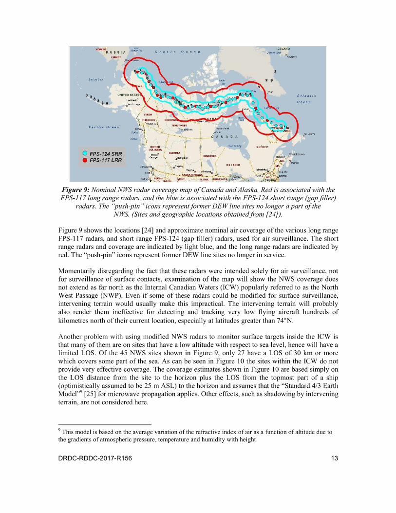
DRDC-RDDC-2017-R156 13
Figure 9: Nominal NWS radar coverage map of Canada and Alaska. Red is associated with the FPS-117 long range radars, and the blue is associated with the FPS-124 short range (gap filler)
radars. The “push-pin” icons represent former DEW line sites no longer a part of the NWS. (Sites and geographic locations obtained from [24]).
Figure 9 shows the locations [24] and approximate nominal air coverage of the various long range FPS-117 radars, and short range FPS-124 (gap filler) radars, used for air surveillance. The short range radars and coverage are indicated by light blue, and the long range radars are indicated by red. The “push-pin” icons represent former DEW line sites no longer in service.
Momentarily disregarding the fact that these radars were intended solely for air surveillance, not for surveillance of surface contacts, examination of the map will show the NWS coverage does not extend as far north as the Internal Canadian Waters (ICW) popularly referred to as the North West Passage (NWP). Even if some of these radars could be modified for surface surveillance, intervening terrain would usually make this impractical. The intervening terrain will probably also render them ineffective for detecting and tracking very low flying aircraft hundreds of kilometres north of their current location, especially at latitudes greater than 74N.
Another problem with using modified NWS radars to monitor surface targets inside the ICW is that many of them are on sites that have a low altitude with respect to sea level, hence will have a limited LOS. Of the 45 NWS sites shown in Figure 9, only 27 have a LOS of 30 km or more which covers some part of the sea. As can be seen in Figure 10 the sites within the ICW do not provide very effective coverage. The coverage estimates shown in Figure 10 are based simply on the LOS distance from the site to the horizon plus the LOS from the topmost part of a ship (optimistically assumed to be 25 m ASL) to the horizon and assumes that the “Standard 4/3 Earth Model”9 [25] for microwave propagation applies. Other effects, such as shadowing by intervening terrain, are not considered here.
9 This model is based on the average variation of the refractive index of air as a function of altitude due to the gradients of atmospheric pressure, temperature and humidity with height
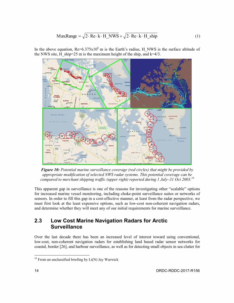
14 DRDC-RDDC-2017-R156
H_shipkRe2H_NWSkRe2RangeMax. (1)
In the above equation, Re=6.375x10⁶ m is the Earth’s radius, H_NWS is the surface altitude of the NWS site, H_ship=25 m is the maximum height of the ship, and k=4/3.
Figure 10: Potential marine surveillance coverage (red circles) that might be provided by appropriate modification of selected NWS radar systems. This potential coverage can be
compared to merchant shipping traffic (upper right) reported during 1 July–31 Oct 2003.10
This apparent gap in surveillance is one of the reasons for investigating other “scalable” options for increased marine vessel monitoring, including choke-point surveillance suites or networks of sensors. In order to fill this gap in a cost-effective manner, at least from the radar perspective, we must first look at the least expensive options, such as low-cost non-coherent navigation radars, and determine whether they will meet any of our initial requirements for marine surveillance.
2.3 Low Cost Marine Navigation Radars for Arctic Surveillance
Over the last decade there has been an increased level of interest toward using conventional, low-cost, non-coherent navigation radars for establishing land based radar sensor networks for coastal, border [26], and harbour surveillance, as well as for detecting small objects in sea clutter for
10 From an unclassified briefing by Lt(N) Jay Warwick
DRDC-RDDC-2017-R156 15
ship self defence [29] and for Search and Rescue (SaR) operations at sea [30]. These types of radar are also in use by organizations such as the Canadian Coast Guard for Vessel Traffic Services (VTS) or—as they are now known—Marine Communications and Traffic Services (MCTS). An X-band radar similar to that purchased for NW is currently in use at the Port-aux-Basques MCTS site along the NL coast of Cabot Strait [31].
Typical basic radar systems originally intended for installation on both small and larger vessels can be purchased for a few tens of thousands of dollars and, with modest low cost upgrades, can provide enhanced capabilities for detection of targets in cluttered environments for SaR. Some of this research has been carried out by Transport Canada at the Transportation Development Centre (TDC) where they were also investigating modifications to enable such radars to identify multi-year sea ice that often poses a significant navigational hazard [31]. Some typical providers of such navigation radar systems include such well know companies as Northrop Grumman (Sperry Marine), Raytheon (Raymarine), Furuno, Lowrance, Sci-tex, Garmin, Simrad and Nobletec.
There are significant benefits to using these types of radars for surveillance, if they are sufficiently capable to meet requirements:
1. The transceiver and antenna systems are relatively simple and therefore easier to repair than most coherent radar systems, thus requiring less skill to maintain in remote locations;
2. The components are commercial-off-the-shelf (COTS) and therefore easily, and readily procured;
3. Because of the relative simplicity of the design, they tend to be more robust and less prone to failure,11 a significant advantage for unmanned sites; e.g., the magnetron used as the RF power amplifier in a non-coherent radar system will typically last over 3000 hours and some over 10000 hours before failure. They are much cheaper ($700–$2000) than a coherent RF power amplifier such as a Travelling Wave Tube (TWT) which often cost over $100k by themselves, and often require long procurement lead times (6 mo. to 1 year). There are also companies that will repair and refurbish damaged magnetrons for about 50% of the original retail cost, i.e., about $300. Typical lifetimes (mean time between failures or MTBF) of airborne radar systems that might be modified for land use are usually less than 400 hours. However, the primary mode of failure for these radars may be due to the gimbals which are highly stressed in airborne use, and might last longer for maritime surveillance. It should also be noted that the MTBF for the FPS-117 and FPS-124 are >1000 hours and >4000 hours respectively, according to the on-line Jane’s Radar and Electronic Warfare Systems.
4. Typical non-coherent marine navigation radars tend to be much less expensive than coherent systems, usually by a factor of 10 to 100. Many coherent radars cost well over 1 million dollars, excluding infrastructure costs. However, it should be noted that with computer and cellular phone technologies driving advances in miniaturized electronic components (e.g., smaller antennas, faster and more powerful processors, and monolithic microwave integrated circuits
11 Possible exceptions might be new lines of radar systems like the Kelvin Hughes SharpEye that employ solid state RF amplifiers that are reported to have a mtbf of up to 50 kh. The SharpEye was not yet on the market at the beginning of the NWTDP project.

16 DRDC-RDDC-2017-R156
(MMIC)), there is a growing trend toward the development of lower-cost coherent radar systems that use Software Defined Radio/Radar (SDR) concepts, high-power solid-state amplifiers and active aperture antennas that will lead to MTBFs well over 10000 hours. SDR concepts also facilitate follow-on system upgrades. At the beginning of the NW project Kelvin Hughes was developing a new solid state, coherent navigational radar called the SharpEye (both X and S-band versions) [32]–[34] which would use lower average and peak powers (<200 W) than the Rutter 100S6 (<300 W average, 25 kW peak) while attaining similar performance. However, they didn’t go to market until more than a year after the start of the project. In addition, when they did come onto the market, they cost about twice as much as a turn-key ship-ready Rutter 100S6 system. So, by purchasing two Rutter systems, the project was able to have a complete fully operational backup system if one had a catastrophic failure.
The maximum detection range of a typical non-coherent marine navigation system depends primarily on the following factors:
Radar RF carrier frequency
Peak transmitting power
Antenna gain
Radar cross section (RCS) of the target
RF Propagation conditions
Relative Antenna to Target geometry (including terrain/sea surface)
P.D.L. Williams et al [35][36] in the mid-1970s used a shore based 9 GHz band HH12 polarized marine radar to measure targets of opportunity at very low grazing angles passing Dungeness, on the north shore of the English Channel. In his experiments the aspect changed from nearly bow-on through broadside to the starboard quarter as the ships passed. Based on the data collected during their experiments and their subsequent analysis they developed a “rule-of-thumb” for the effective RCS of extended merchant vessel targets that was a simple function of the ship’s gross tonnage. This empirical estimate of the RCS was given by the following relationship:
8.4∙log10(T) dB m2 ≤ RCS ≤11.9∙log10(T) dB m2 (2)
This is based on the information shown in Table 2 and plotted in Figure 11. This empirical formula, along with the RF SIESTA software allows one to estimate the range detection and coverage at a given sensor location. Figure 12 shows a radar range coverage map based on SIESTA predictions for a 25 kW X-band radar placed on top of Cape Liddon at 74.62861°N, 91.168333°W at an altitude of 320 m ASL. The green dots show the approximate maximum range to detect vessels like those shown on the right, based on their average RCS as predicted by (2).
Annex D contains information on typical types and sizes of maritime vessels that have been observed to operate within the waters of the NWP over several years from 2003 to 2008. The information was compiled from reports used to produce the Recognized Maritime Picture (RMP) during that period, as well as analysis of shipping activity by Joint Task Force North (JTFN) J2
12 Horizontal polarization on transmit and horizontal polarization on receive.

DRDC-RDDC-2017-R156 17
[37], and from sources on the Internet. It is useful to compare this information to some of the vessels observed in the vicinity of Halifax Harbour and NESTRA during the trials in 2008, some of which will be shown in Sections 6.1.2 and 6.1.3.
The average RCS at X band for various vessel sizes, based on empirical observations, is given by the range of values shown in Table 2. Based on this information, a small craft such as a small inshore fishing vessel, up to a small tug boat may have an RCS between 5 and 15 dBsm, a small vessel under 300 tons would be between 15 and 20 dBsm, a large vessel between 300 and 20,000 tons would have an RCS between 20 and 45 dBsm and a very large ship would have an RCS between 45 and 75 dBsm. Note, that all of the values given above are average values, not peaks that exceed the average by 20 or 30 dBsm depending on the ship configuration or relative aspect with respect to the radar. As will be shown in Sections 6.1.2 and 6.1.3 this full extreme of vessel sizes was observed and tracked, with varying degrees of success, at the NESTRA 2008 Trials.
Table 2: Empirical Ship RCS estimates related to ship size and type [35]. Ship Type Ref
. GT
(tons) Length LOA (m)
RCS min.
(dB m2)
RCS max.
(dB m2)
Deviation from LHS of
Eq. 1 (Max. dB)
Deviation from RHS of
Eq. 1 (Min. dB)
Merchant Ships Inshore F/V 13 5 8.5 5 10 1.7 -0.9 Small coaster 18 225 42.6 14 29 1.0 -5.8 Coaster 3 500 54.9 17 33 0.9 -5.7 Coaster 1 500 54.9 25 36 3.9 2.3 Coaster 16 500 56.7 30 41 8.9 7.3 Large Coaster 2 1000 67.1 30 37 1.3 4.8 Collier 4 1570 73.5 25 33 -5.0 -1.8 Cargo Liner 10 5000 114.0 40.5 42 -2.0 9.44 Cargo Liner 11 8000 136.6 36 42 -4.4 3.2
Bulk Carrier 6 8200 166.4 28 41 -5.6 -4.9
Cargo 9 9400 154.5 32 41 -63 -1.4
Cargo 7 10430 166.1 28.5 42 -5.8 -5.3
Bulk Carrier 12 17500 198.1 30 45 -5.5 -5.6
Ore Carrier 8 25400 205.7 32 45 -7.4 -5.0 Container Carrier w/large deck cargo
9 26436 208.8 40 48 -4.6 2.9
Medium Tanker 15 32500 221 47 59 53 9.1 Medium Tanker 17 44700 251.2 43 62 6.7 3.9 Warship Frigate 14 2000 103 38 50 10.7 10.3
GT=Gross Tonnage. Coaster= coastal trading vessel; usually shallow hulled, small cargo ships, often containerships, that run on feeder routes along the coast. F/V=fishing vessel. Collier=an historical term used to describe a bulk cargo ship designed to carry coal.

18 DRDC-RDDC-2017-R156
Figure 11: Empirical data showing effective RCS of various merchant ship sizes when viewed at low grazing angles with a marine navigation radar similar to the one used at NESTRA [35][36].
Figure 12: SIESTA range and coverage predictions for a 25kW X-band radar placed on top of
Cape Liddon at 74.62861°N, 91.168333°W at an altitude of 320 m ASL. The green dots show the approximate maximum range to detect the vessels on the right, for their average RCS.
100 101 102 103 104 1050
10
20
30
40
50
60
70
Cargo Volume (gross tons)
RC
S (d
Bm2 )
Williams' Ship RCS Measurements

DRDC-RDDC-2017-R156 19
A practical lower limit on RCS for sea going vessels is provided by regulations adhered to by countries that follow the Safety Of Life At Sea (SOLAS) Conference: all ships within the SOLAS Convention built after 2002 and under 150 gt, are required to carry a radar reflector or other means to enhance detectability to marine radars at 3 and 9 GHz. The specific regulation, i.e., Chapter V, Regulation 19.2.1.7 [38][39] states that a ship shall have:
“if less than 150 gross tonnage, and if practicable, a radar reflector, or other means, to enable detection by ships navigating by radar at both 9 and 3 GHz.”
Further guidance on implementing this capability is provided by British Standards BS EN ISO 8729:1998 (ISO 8729:1997) [39] and later versions of the ISO standard. The test standard for type approval of passive or active radar target enhancers (RTE) according to ISO 8927:1997 is that they meet the following criteria:
1. Provide a peak RCS of at least 10 m2 (10 dBsm);
2. Provide an RCS of at least 2.5 m² (4 dBsm) over an azimuth angle of at least 240° when the reflector is vertical (i.e., not heeled over);
3. Provide an RCS of at least 0.625 m² over an azimuth angle of at least 240° for angles of heel up to +/- 15°.
An evaluation and comparison [40] of several passive RTE and one active RTE commonly used on small boats in British waters was carried out in the UK by Qinetiq in 2007 at the request of the Marine Accident Investigation Branch (MAIB). The MAIB commissioned the study following the loss of a yacht named ‘Ouzo’ in August 2006. That study was particularly relevant to this report because their modelling was based on a 25 kW X-band BridgeMaster transceiver and antenna with very similar characteristics to the one used in the NESTRA trials.
This requirement also applies to any passenger vessels irrespective of size. For vessels over 15 m in length, the reflector should be located on a mast or in the rigging of the ship at a height of 4 m or higher, if possible; however, for vessels less than 15 m, they should be fitted with the most efficient reflector that the vessel can accommodate.
One caveat that must be considered is the strong possibility that small vessels such as sailboats may not always have such corner reflectors or other RTE devices deployed at all times, as suggested by IMO and other safety standards organizations. For various reasons, they might only deploy these devices during periods of poor visibility such as during foggy conditions, or at night.
Since most maritime vessel traffic in the Arctic maintain speeds that are significantly less than 100 knots (typically <20 knots) then if the vessels of interest (VOI) are large enough and/or are moving slowly enough, scan-to-scan video integration can be performed to reduce the effects of sea-clutter and improve the signal to noise ratio for vessel detection and tracking. This is the basis of the scan averaging technique employed by Rutter in their 100S6 radar system. This scan averaging technique is also potentially useful for detecting and tracking ice flows through Barrow Strait or other locations, which might aid ship navigation in the area. The same technique may also assist with oil-spill detection [42]–[55] at ranges less than 10 km.
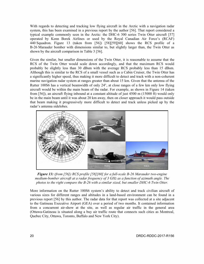
20 DRDC-RDDC-2017-R156
With regards to detecting and tracking low flying aircraft in the Arctic with a navigation radar system, this has been examined in a previous report by the author [56]. That report considered a typical example commonly seen in the Arctic: the DHC-6 300 series Twin Otter aircraft [57] operated by Kenn Borek Airlines or used by the Royal Canadian Air Force’s (RCAF) 440 Squadron. Figure 13 (taken from [56]) [58][59][60] shows the RCS profile of a B-26 Marauder bomber with dimensions similar to, but slightly larger than, the Twin Otter as shown by the aircraft comparison in Table 3 [56].
Given the similar, but smaller dimensions of the Twin Otter, it is reasonable to assume that the RCS of the Twin Otter would scale down accordingly, and that the maximum RCS would probably be slightly less than 30 dBsm with the average RCS probably less than 15 dBsm. Although this is similar to the RCS of a small vessel such as a Cabin Cruiser, the Twin Otter has a significantly higher speed, thus making it more difficult to detect and track with a non-coherent marine navigation radar system at ranges greater than about 15 km. Given that the antenna of the Rutter 100S6 has a vertical beamwidth of only 24, at close ranges of a few km only low flying aircraft would be within the main beam of the radar. For example, as shown in Figure 14 (taken from [56]), an aircraft flying inbound at a constant altitude of just 4500 m (15000 ft) would only be in the main beam until it was about 20 km away, then on closer approach it would pass outside that beam making it progressively more difficult to detect and track unless picked up by the radar’s antenna sidelobes.
Figure 13: (from [56]) RCS profile [58][60] for a full-scale B-26 Marauder two-engine
medium-bomber aircraft at a radar frequency of 3 GHz as a function of azimuth angle. The photos to the right compare the B-26 with a similar sized, but smaller DHC-6 Twin Otter.
More information on the Rutter 100S6 system’s ability to detect and track civilian aircraft of various sizes for different ranges and altitudes in a land-based environment can be found in a previous report [56] by this author. The radar data for that report was collected at a site adjacent to the Gatineau Executive Airport (GEA) over a period of two months. It contained information from a concurrent air-show at the site, as well as regular air traffic in the general area (Ottawa-Gatineau is situated along a buy air traffic route that connects such cities as Montreal, Quebec City, Ottawa, Toronto, Buffalo and New York City).

DRDC-RDDC-2017-R156 21
Figure 14: (from [56]) Low flying aircraft geometry with respect to
a Rutter 100S6 radar on Cape Liddon.
Table 3: Chart comparing a Kenn Borek Airlines Twin Otter DHC-6 [57] to a B-26 Marauder [59].
Parameter Twin Otter (DHC-6 300 series) Martin B-26 Marauder Bomber Length 51 ft 9 in (15.77 m) 58 ft 3 in (17.8 m) Wingspan 65 ft (19.8 m) 71 ft 0 in (21.65 m) Height 19 ft 6 in (5.9 m) 21 ft 6 in (6.55 m) Wing area 420 ft² (39 m²) 658 ft2 (61.1 m2) Aileron area 33 Flap area 112 Fin area 48 Rudder area 34 Elevator area 100 Empty weight 7,000 lb (3,363 kg) to 8,000 lb
(3,628 kg) 24,000 lb (11,000 kg)
Speed 143–183 kn 216–287 kn Operational Ceiling (2 engine)
6780 m (26700 ft) 6400 m (21000 ft)
2.4 High Frequency Surface Wave Radar (HFSWR) At the beginning of the NW project 2006–2007, the HFSWR was the only sensor in Canada capable of long range, persistent, Over-the Horizon (OTH) ship detection; two demonstration systems existed that were being used operationally, for a short period, to provide input to the RMP. The two sites were on the coast of Newfoundland, at Cape Race and Cape Bonavista. However, the two sites were decommissioned, partly due to fears about interference with other communications systems in the 3–15 MHz band, and a new project was undertaken to address such issues. The new project, which was called Persistent Active Surveillance of the Exclusive-Economic-Zone (PASE) came to a successful conclusion in 2015.

22 DRDC-RDDC-2017-R156
As part of its initial sensor evaluation phase for the Arctic, the NW project considered testing a portable version of the HFSWR that was available at DRDC Ottawa. However, after consulting the scientist responsible for the device, Dr. R. Riddolls, the idea was quickly abandoned for the following reasons:
1. Since the HFSWR is primarily designed for long range OTH ship detection and tracking, its usefulness or suitability as a choke point sensor may be doubtful given that a conventional maritime radar with a much smaller footprint, and greater azimuth resolution, might be used instead.
2. The HFSWR radar would consume about 15 kW, including shelter heating. This would require about 30–40 gallons of diesel/day.
3. Depending on the gain and directionality required of the antenna array, the real-estate footprint of the system might be a logistical problem at the remote site (the PASE demonstration array is over 500 m long and 50 m wide).
4. Providing physical security for the transmitter and receiver arrays for unattended operation would be difficult given the harsh environment, and wildlife issues (e.g., polar bears).
5. For unattended operation, a Ku-band satellite communication system would need to be established. This would cost around $30k to set up and $1500/month to run. The speeds available at the time were typically 128kbit/s up and 512kbit/s down, which is fast enough for unattended operation, and possibly retrieval of raw data from the local hard drive. Thus communications costs will be about $40k.
6. With regards to the radar hardware itself, some reconfiguration would be needed to allow for unattended operation. The portable radar system was configured to send plots to an IP socket connection and the tracker typically ran in a remote location, such as Raytheon in Waterloo, Ontario. However, there was no way to remotely monitor the health of the hardware in the transportable HF radar. For the East Coast systems, a condition monitoring system (CMS) was devised that consists of populating the hardware with sensors, and running the sensors into a data acquisition (DAQ) card on a PC running Labview. The effort for installing a CMS in the transportable radar was estimated to be in the $150k range.
7. The transportable radar contained only a single frequency generator (as opposed to two in each of the East Coast systems) and one 16-channel receiver set (as opposed to two sets of 16-channels in each of the East Coast systems). The problem with single frequency operation is that there are blind velocities corresponding to the Doppler frequencies of the Ocean Bragg scatter lines. Correcting this deficiency would either involve building a second frequency upgrade for the transportable system (estimated to cost $700k) to allow pulse-to-pulse dual frequency, or going with a scheme where frequencies were switched on a dwell-to-dwell basis (perhaps a $200k effort to get working). Solutions would depend on the available funding.
8. A further issue was that the transportable system operated at 12–18 MHz. Depending on ship targets and ranges, a preferable band would probably be in the 2–6 MHz range. This would require building some sort of new transmit antenna. The log-periodic antennas on the east coast are rather large, and cost around $200k to build/install. However, if you choose not to go with dual frequency to save money, you could settle for a narrowband monopole antenna.

DRDC-RDDC-2017-R156 23
This could be as simple as a few assembled tower sections, driven at resonance, which might cost $50k to install.
9. At the time of consideration, the shelter for the back-end electronics was a modified shipping container that weighted several tons, which presented a considerable logistical/cost challenge for deployment to a remote arctic site;
10. The overall cost, excluding transportation and power generation, and just settling for a single-frequency operation, would amount to at least $600k.
These issues coupled with other unknowns, such as the possible effects of auroral and ionospheric interference, resulted in the decision to discontinue any serious consideration of using this system.
2.5 Airborne Radar Systems and Platforms
Airborne sensor systems, whether they are carried by manned or unmanned fixed wing aircraft or lighter than air (LTA) vessels would present logistical (e.g., piloting, support, maintenance) and/or cost issues that would exceed the capacity of the NW project. Also, with the possible exception of aerostats, time-on-station and persistence would also be a difficulty. Table 4 provides some information and estimates of cost per flight hour of each of the systems. Table 5 provides a few examples of solid-state coherent airborne radar systems along with some of their specifications, including approximate unit costs for two of the systems. The L-88 variants are usually on an aerostat whereas the SeaSpray variants have been used in aerostats, fixed and rotary wing manned aircraft, and MALE UAVs (e.g., Predator).
Table 4: Cost/Endurance comparison for persistent surveillance platforms based on information up to 2007 [61][62].
PLATFORM COST/FLIGHT HOURS ($103 USD)
ENDURANCE (UNREFUELLED)
AWACS* 20 11 hrs
JSTARS* 20 11hrs
E-2C* 18.7 4.7 hrs
Global Hawk* 26.5 35 hrs
Predator* 5.0 40 hrs
420K TARS* 0.3–0.5 15–30 days (barring weather)
Manned Airship (e.g., Zeppelin) 1.8 (with 1yr lease) Few days (payload/fuel restricted)
CP-140 Aurora (Maritime Patrol Aircraft)†
> 10 10–14
Provincial Aerospace Ltd (King Air 220+sensor suite)†
~1.5 ~5 hours
* US systems † Does not assume Arctic deployment, in which case costs would increase.

24 DRDC-RDDC-2017-R156
Table 5: Some examples of solid state coherent airborne radar systems; the L-88 variants are usually on an aerostat whereas the SeaSpray variants have been used in aerostats, fixed and
rotary wing manned aircraft, and UAVs (e.g., Predator).
Radar L-88A L-88(V)3 SeaSpray 5000E Seaspray 7500E Manufacturer Lockheed Martin Lockheed Martin Selex Galileo Selex Galileo Type Coherent solid
state transceiver with parabolic antenna
Coherent solid state transceiver with parabolic antenna
Coherent Active Electronically Scanned Array (AESA) radar
Coherent AESA radar
Frequency L-band (1200–1400 MHz)
L-band (1200–1400 MHz)
X-band (8–12 GHz)
X-band (8–12 GHz)
Antenna dimensions (m)
Width: 7.63 Height: 3.96
Width: 7.63 Height: 3.96
Width:0.5 or 0.43 Height:0.26 or 0.28 Depth:0.21 or 0.14
Weight (kg) 1021 590 45 110 Power 16.6 kW peak 8.5 kW peak Nominal Detection Range
370 km (for direct LOS to 1 m2 target at 3660 m altitude)
370 km (for direct LOS to 1 m2 target at 3660 m altitude)
185.2 km (for direct LOS to 1 m2)
592.6 km (for direct LOS to 1 m2)
MTBF 1000 h 1000 h 2000 h >2000 h Modes of operation
Long and short range pulses, with Linear FM (chirp) pulse compression, MTI
Long and short range pulses, with Linear FM (chirp) pulse compression, MTI
Multifunction, SAR, ISAR MTI (air to air), GMTI (air to ground), track while scan
Multifunction, SAR, ISAR MTI (air to air), GMTI (air to ground), track while scan
Beam Characteristics
2D search Elevation: 5° cosec2. Azimuth: 2.3° Scanning: mechanical 360° azimuth scan
2D search Elevation: 5° cosec2. Azimuth: 2.3° Scanning: mechanical 360° azimuth scan
3D search Pencil Beam; Scanning: Vertical Electronic Scan and mechanical tilt; mechanical azimuth scan
3D search Pencil Beam; Scanning: Vertical Electronic Scan and mechanical tilt; mechanical azimuth scan
Cost per unit (million $US)
~$4 $2 to $3
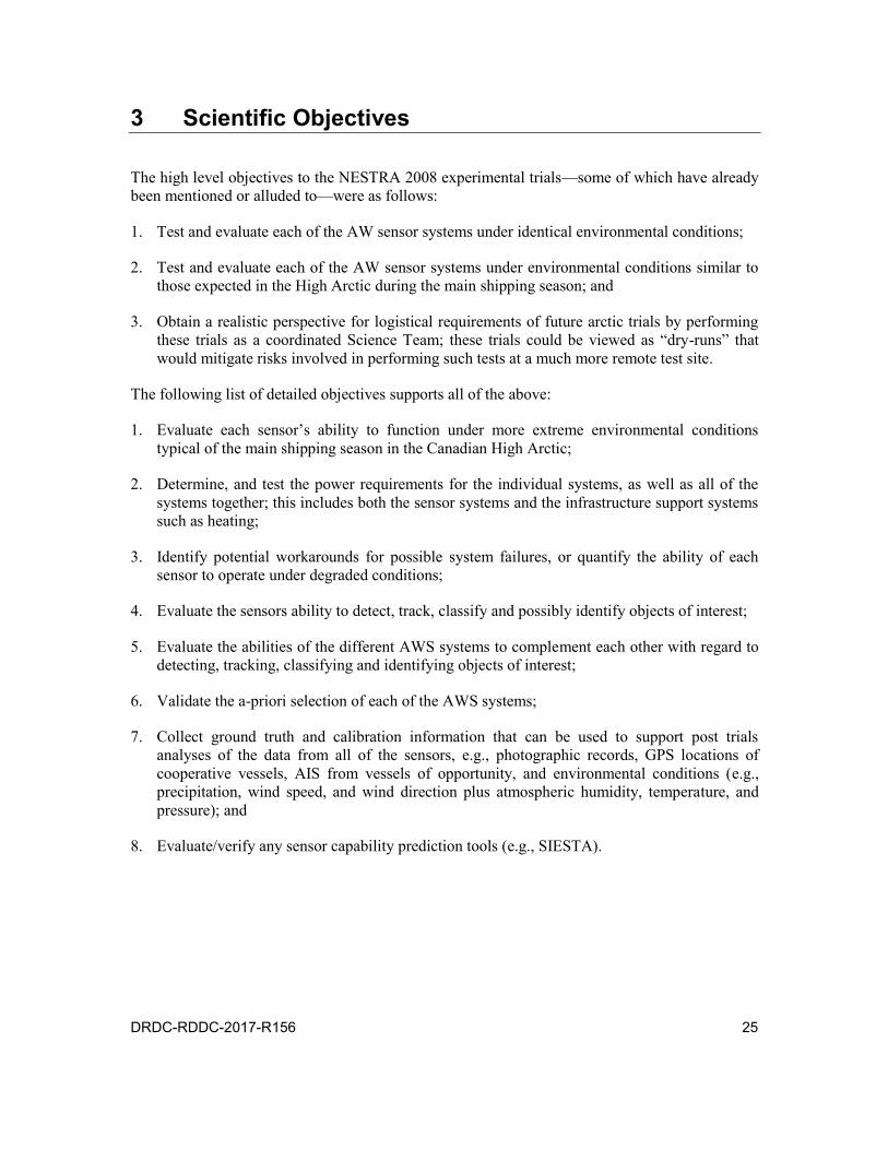
DRDC-RDDC-2017-R156 25
3 Scientific Objectives
The high level objectives to the NESTRA 2008 experimental trials—some of which have already been mentioned or alluded to—were as follows:
1. Test and evaluate each of the AW sensor systems under identical environmental conditions;
2. Test and evaluate each of the AW sensor systems under environmental conditions similar to those expected in the High Arctic during the main shipping season; and
3. Obtain a realistic perspective for logistical requirements of future arctic trials by performing these trials as a coordinated Science Team; these trials could be viewed as “dry-runs” that would mitigate risks involved in performing such tests at a much more remote test site.
The following list of detailed objectives supports all of the above:
1. Evaluate each sensor’s ability to function under more extreme environmental conditions typical of the main shipping season in the Canadian High Arctic;
2. Determine, and test the power requirements for the individual systems, as well as all of the systems together; this includes both the sensor systems and the infrastructure support systems such as heating;
3. Identify potential workarounds for possible system failures, or quantify the ability of each sensor to operate under degraded conditions;
4. Evaluate the sensors ability to detect, track, classify and possibly identify objects of interest;
5. Evaluate the abilities of the different AWS systems to complement each other with regard to detecting, tracking, classifying and identifying objects of interest;
6. Validate the a-priori selection of each of the AWS systems;
7. Collect ground truth and calibration information that can be used to support post trials analyses of the data from all of the sensors, e.g., photographic records, GPS locations of cooperative vessels, AIS from vessels of opportunity, and environmental conditions (e.g., precipitation, wind speed, and wind direction plus atmospheric humidity, temperature, and pressure); and
8. Evaluate/verify any sensor capability prediction tools (e.g., SIESTA).
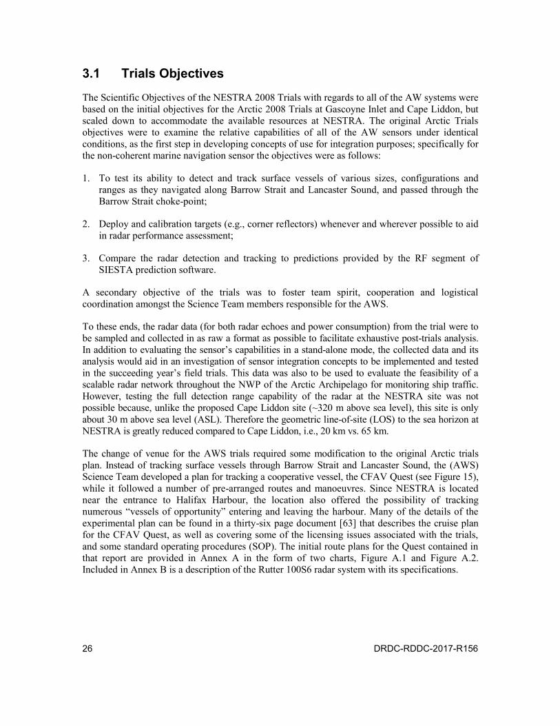
26 DRDC-RDDC-2017-R156
3.1 Trials Objectives
The Scientific Objectives of the NESTRA 2008 Trials with regards to all of the AW systems were based on the initial objectives for the Arctic 2008 Trials at Gascoyne Inlet and Cape Liddon, but scaled down to accommodate the available resources at NESTRA. The original Arctic Trials objectives were to examine the relative capabilities of all of the AW sensors under identical conditions, as the first step in developing concepts of use for integration purposes; specifically for the non-coherent marine navigation sensor the objectives were as follows:
1. To test its ability to detect and track surface vessels of various sizes, configurations and ranges as they navigated along Barrow Strait and Lancaster Sound, and passed through the Barrow Strait choke-point;
2. Deploy and calibration targets (e.g., corner reflectors) whenever and wherever possible to aid in radar performance assessment;
3. Compare the radar detection and tracking to predictions provided by the RF segment of SIESTA prediction software.
A secondary objective of the trials was to foster team spirit, cooperation and logistical coordination amongst the Science Team members responsible for the AWS.
To these ends, the radar data (for both radar echoes and power consumption) from the trial were to be sampled and collected in as raw a format as possible to facilitate exhaustive post-trials analysis. In addition to evaluating the sensor’s capabilities in a stand-alone mode, the collected data and its analysis would aid in an investigation of sensor integration concepts to be implemented and tested in the succeeding year’s field trials. This data was also to be used to evaluate the feasibility of a scalable radar network throughout the NWP of the Arctic Archipelago for monitoring ship traffic. However, testing the full detection range capability of the radar at the NESTRA site was not possible because, unlike the proposed Cape Liddon site (~320 m above sea level), this site is only about 30 m above sea level (ASL). Therefore the geometric line-of-site (LOS) to the sea horizon at NESTRA is greatly reduced compared to Cape Liddon, i.e., 20 km vs. 65 km.
The change of venue for the AWS trials required some modification to the original Arctic trials plan. Instead of tracking surface vessels through Barrow Strait and Lancaster Sound, the (AWS) Science Team developed a plan for tracking a cooperative vessel, the CFAV Quest (see Figure 15), while it followed a number of pre-arranged routes and manoeuvres. Since NESTRA is located near the entrance to Halifax Harbour, the location also offered the possibility of tracking numerous “vessels of opportunity” entering and leaving the harbour. Many of the details of the experimental plan can be found in a thirty-six page document [63] that describes the cruise plan for the CFAV Quest, as well as covering some of the licensing issues associated with the trials, and some standard operating procedures (SOP). The initial route plans for the Quest contained in that report are provided in Annex A in the form of two charts, Figure A.1 and Figure A.2. Included in Annex B is a description of the Rutter 100S6 radar system with its specifications.
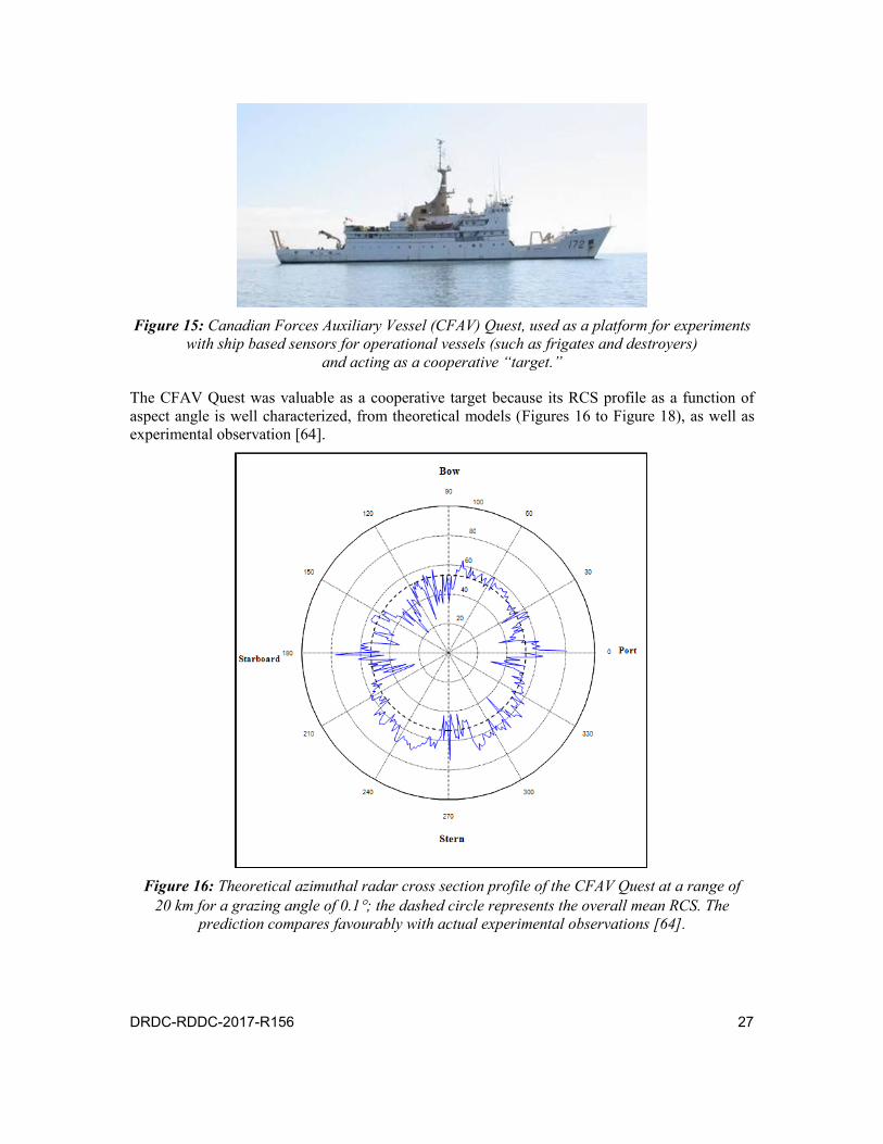
DRDC-RDDC-2017-R156 27
Figure 15: Canadian Forces Auxiliary Vessel (CFAV) Quest, used as a platform for experiments
with ship based sensors for operational vessels (such as frigates and destroyers) and acting as a cooperative “target.”
The CFAV Quest was valuable as a cooperative target because its RCS profile as a function of aspect angle is well characterized, from theoretical models (Figures 16 to Figure 18), as well as experimental observation [64].
Figure 16: Theoretical azimuthal radar cross section profile of the CFAV Quest at a range of
20 km for a grazing angle of 0.1; the dashed circle represents the overall mean RCS. The prediction compares favourably with actual experimental observations [64].
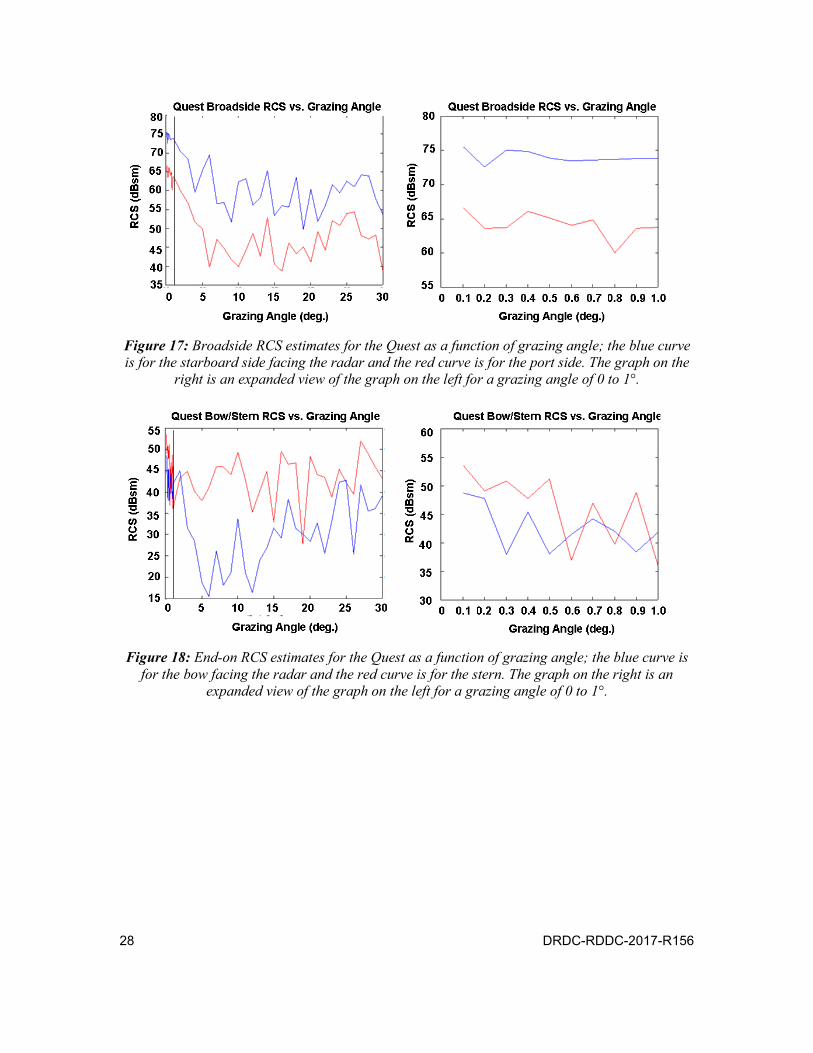
28 DRDC-RDDC-2017-R156
Figure 17: Broadside RCS estimates for the Quest as a function of grazing angle; the blue curve is for the starboard side facing the radar and the red curve is for the port side. The graph on the
right is an expanded view of the graph on the left for a grazing angle of 0 to 1°.
Figure 18: End-on RCS estimates for the Quest as a function of grazing angle; the blue curve is
for the bow facing the radar and the red curve is for the stern. The graph on the right is an expanded view of the graph on the left for a grazing angle of 0 to 1°.
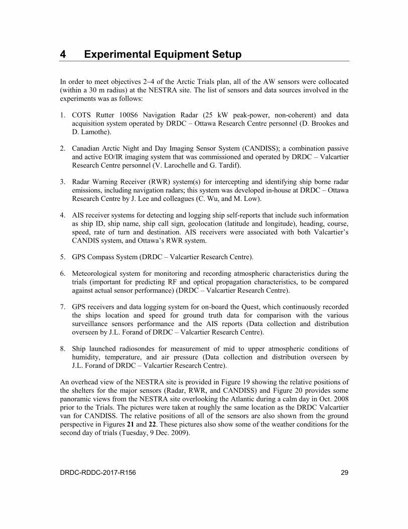
DRDC-RDDC-2017-R156 29
4 Experimental Equipment Setup
In order to meet objectives 2–4 of the Arctic Trials plan, all of the AW sensors were collocated (within a 30 m radius) at the NESTRA site. The list of sensors and data sources involved in the experiments was as follows:
1. COTS Rutter 100S6 Navigation Radar (25 kW peak-power, non-coherent) and data acquisition system operated by DRDC – Ottawa Research Centre personnel (D. Brookes and D. Lamothe).
2. Canadian Arctic Night and Day Imaging Sensor System (CANDISS); a combination passive and active EO/IR imaging system that was commissioned and operated by DRDC – Valcartier Research Centre personnel (V. Larochelle and G. Tardif).
3. Radar Warning Receiver (RWR) system(s) for intercepting and identifying ship borne radar emissions, including navigation radars; this system was developed in-house at DRDC – Ottawa Research Centre by J. Lee and colleagues (C. Wu, and M. Low).
4. AIS receiver systems for detecting and logging ship self-reports that include such information as ship ID, ship name, ship call sign, geolocation (latitude and longitude), heading, course, speed, rate of turn and destination. AIS receivers were associated with both Valcartier’s CANDIS system, and Ottawa’s RWR system.
5. GPS Compass System (DRDC – Valcartier Research Centre).
6. Meteorological system for monitoring and recording atmospheric characteristics during the trials (important for predicting RF and optical propagation characteristics, to be compared against actual sensor performance) (DRDC – Valcartier Research Centre).
7. GPS receivers and data logging system for on-board the Quest, which continuously recorded the ships location and speed for ground truth data for comparison with the various surveillance sensors performance and the AIS reports (Data collection and distribution overseen by J.L. Forand of DRDC – Valcartier Research Centre).
8. Ship launched radiosondes for measurement of mid to upper atmospheric conditions of humidity, temperature, and air pressure (Data collection and distribution overseen by J.L. Forand of DRDC – Valcartier Research Centre).
An overhead view of the NESTRA site is provided in Figure 19 showing the relative positions of the shelters for the major sensors (Radar, RWR, and CANDISS) and Figure 20 provides some panoramic views from the NESTRA site overlooking the Atlantic during a calm day in Oct. 2008 prior to the Trials. The pictures were taken at roughly the same location as the DRDC Valcartier van for CANDISS. The relative positions of all of the sensors are also shown from the ground perspective in Figures 21 and 22. These pictures also show some of the weather conditions for the second day of trials (Tuesday, 9 Dec. 2009).

30 DRDC-RDDC-2017-R156
In order to maintain minimal interference with the NESTRA facilities during the Trials, most of the AW sensors and equipment were sheltered in vehicles either belonging to DRDC, or rented for this purpose. The only building facilities and resources that were needed from NESTRA were: external power to the vehicles/shelters, access to heated shop facilities for temporary indoor shelter of equipment and personnel, and washroom facilities. NESTRA also graciously loaned the trials team a marine radio for communication and coordination with the CFAV Quest and access to a small meeting room for a post trials wash-up meeting.
In anticipation of these trials, the team developed a communication plan which identified offices of primary interest (OPI), the points of contact (POC), and the standard operating procedures for point to point communications (e.g., ship-to-shore). Under this plan, one of the duties of project’s Lead Scientist (D. Brookes), and as the trials coordinator, was to warn the airstrip at Shearwater, and the Operations Centre at Trinity via telephone prior to any plans to start using the active laser imaging system for CANDISS. This allowed them to either warn the NESTRA Trials Team against proceeding due to emergencies or other unavoidable circumstances, or to warn aircraft out of the immediate risk area as originally planned. This was required because the active imaging system of CANDISS employs a laser that is not eye safe within a nominal optical hazard distance (NOHD) of about 700 m, or an extended optical hazard zone (EOHD) of about 3 km. According to the communications plan, Mr Brookes and Dr. Forand also served as the local points of contact for coordinating activities at, and between, NESTRA and the Quest respectively.
As part of the initial radar set-up, the transceiver and antenna were bolted to a 4 ft by 6 ft piece of ¾ inch plywood, then deployed to the top of the cargo box of the truck and held securely in place with two guy ropes on each side, as shown in Figure 20. Despite wind gusts as high as 70 kph (shown later in Figure 37), the radar antenna remained securely fastened. The placement of the radar transceiver on top of the truck’s cargo container minimized exposure of ground personnel to the radar’s main beam during operation. A photograph plus a descriptive diagram of the trucks configuration is shown in Figure 23. As part of the Standard Operating Procedures (SOP) to ensure personnel safety, an orange strobe light with a magnetic base was placed on the truck cab to act as a warning beacon. It was turned on whenever the radar was in operation (see Figure 23).
The physical orientation or the antenna base containing the transceiver and drive motor was important because it determined the “apparent” North-Up for the radar display while it was in operation. However, due to difficulties in accurately aligning the system prior to operation, it was decided that the display orientation would be calibrated in post processing. This would be accomplished by using the location of known landmarks, such as several buoys in the NESTRA AOR, relative to the radar’s GPS location.

DRDC-RDDC-2017-R156 31
Figure 19: Area around Halifax Harbour showing the location of Osborne Head (inset upper left) and NESTRA (inset upper right); the
NESTRA photo also shows the relative locations of the Radar/RWR truck and the CANDISS truck indicated by white rectangles.

32 DRDC-RDDC-2017-R156
Figure 20: Panoramic photos of the NESTRA site overlooking the Atlantic during a calm day in Oct. 2008 prior to the Trials. The pictures
were taken at roughly the same location as the DRDC Valcartier van for CANDISS.

DRDC-RDDC-2017-R156 33
Figure 21: One view of the Radar/RWR truck showing the set-up of the RWR, Radar and
communications antennas. The photo was taken on the relatively calm Tues. morning of Dec. 9 after the previous night’s storm.
Figure 22: A view of relative set-up for all of the AW sensors at NESTRA (excluding AIS)
on the morning of Tues. 9 Dec (photo by the author).
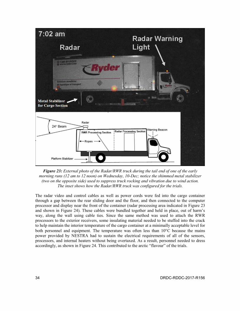
34 DRDC-RDDC-2017-R156
Figure 23: External photo of the Radar/RWR truck during the tail end of one of the early
morning runs (12 am to 12 noon) on Wednesday, 10-Dec; notice the shimmed metal stabilizer (two on the opposite side) used to suppress truck rocking and vibration due to wind action.
The inset shows how the Radar/RWR truck was configured for the trials.
The radar video and control cables as well as power cords were fed into the cargo container through a gap between the rear sliding door and the floor, and then connected to the computer processor and display near the front of the container (radar processing area indicated in Figure 23 and shown in Figure 24). These cables were bundled together and held in place, out of harm’s way, along the wall using cable ties. Since the same method was used to attach the RWR processors to the exterior receivers, some insulating material needed to be stuffed into the crack to help maintain the interior temperature of the cargo container at a minimally acceptable level for both personnel and equipment. The temperature was often less than 10C because the mains power provided by NESTRA had to sustain the electrical requirements of all of the sensors, processors, and internal heaters without being overtaxed. As a result, personnel needed to dress accordingly, as shown in Figure 24. This contributed to the arctic “flavour” of the trials.
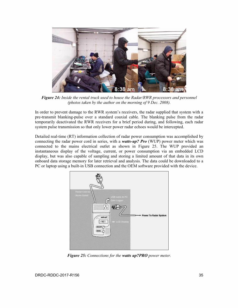
DRDC-RDDC-2017-R156 35
Figure 24: Inside the rental truck used to house the Radar/RWR processors and personnel
(photos taken by the author on the morning of 9 Dec. 2008).
In order to prevent damage to the RWR system’s receivers, the radar supplied that system with a pre-transmit blanking-pulse over a standard coaxial cable. The blanking pulse from the radar temporarily deactivated the RWR receivers for a brief period during, and following, each radar system pulse transmission so that only lower power radar echoes would be intercepted.
Detailed real-time (RT) information collection of radar power consumption was accomplished by connecting the radar power cord in series, with a watts-up? Pro (WUP) power meter which was connected to the mains electrical outlet as shown in Figure 25. The WUP provided an instantaneous display of the voltage, current, or power consumption via an embedded LCD display, but was also capable of sampling and storing a limited amount of that data in its own onboard data storage memory for later retrieval and analysis. The data could be downloaded to a PC or laptop using a built-in USB connection and the OEM software provided with the device.
Figure 25: Connections for the watts up?PRO power meter.
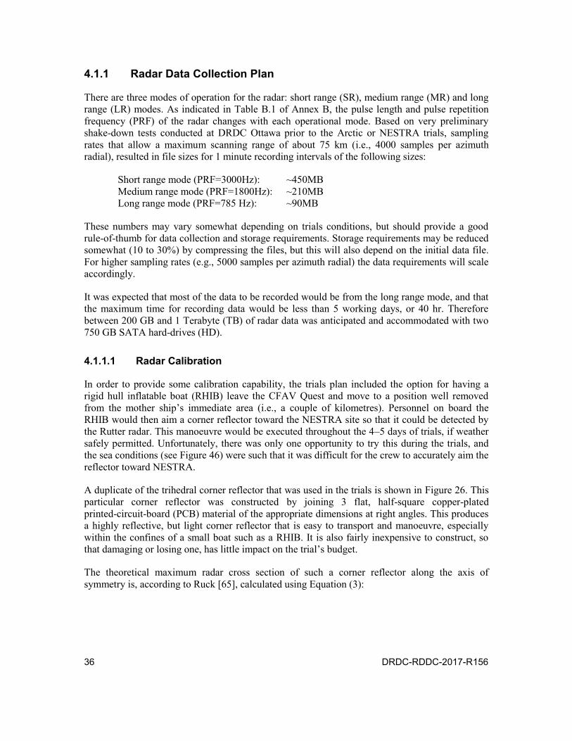
36 DRDC-RDDC-2017-R156
4.1.1 Radar Data Collection Plan
There are three modes of operation for the radar: short range (SR), medium range (MR) and long range (LR) modes. As indicated in Table B.1 of Annex B, the pulse length and pulse repetition frequency (PRF) of the radar changes with each operational mode. Based on very preliminary shake-down tests conducted at DRDC Ottawa prior to the Arctic or NESTRA trials, sampling rates that allow a maximum scanning range of about 75 km (i.e., 4000 samples per azimuth radial), resulted in file sizes for 1 minute recording intervals of the following sizes:
Short range mode (PRF=3000Hz): ~450MB Medium range mode (PRF=1800Hz): ~210MB Long range mode (PRF=785 Hz): ~90MB
These numbers may vary somewhat depending on trials conditions, but should provide a good rule-of-thumb for data collection and storage requirements. Storage requirements may be reduced somewhat (10 to 30%) by compressing the files, but this will also depend on the initial data file. For higher sampling rates (e.g., 5000 samples per azimuth radial) the data requirements will scale accordingly.
It was expected that most of the data to be recorded would be from the long range mode, and that the maximum time for recording data would be less than 5 working days, or 40 hr. Therefore between 200 GB and 1 Terabyte (TB) of radar data was anticipated and accommodated with two 750 GB SATA hard-drives (HD).
4.1.1.1 Radar Calibration
In order to provide some calibration capability, the trials plan included the option for having a rigid hull inflatable boat (RHIB) leave the CFAV Quest and move to a position well removed from the mother ship’s immediate area (i.e., a couple of kilometres). Personnel on board the RHIB would then aim a corner reflector toward the NESTRA site so that it could be detected by the Rutter radar. This manoeuvre would be executed throughout the 4–5 days of trials, if weather safely permitted. Unfortunately, there was only one opportunity to try this during the trials, and the sea conditions (see Figure 46) were such that it was difficult for the crew to accurately aim the reflector toward NESTRA.
A duplicate of the trihedral corner reflector that was used in the trials is shown in Figure 26. This particular corner reflector was constructed by joining 3 flat, half-square copper-plated printed-circuit-board (PCB) material of the appropriate dimensions at right angles. This produces a highly reflective, but light corner reflector that is easy to transport and manoeuvre, especially within the confines of a small boat such as a RHIB. It is also fairly inexpensive to construct, so that damaging or losing one, has little impact on the trial’s budget.
The theoretical maximum radar cross section of such a corner reflector along the axis of symmetry is, according to Ruck [65], calculated using Equation (3):

DRDC-RDDC-2017-R156 37
4
2
24
24
/4RCS
a
L
(3)
In Equation (3) above, L is the length of one of the corner edges, a is the length of one of the aperture edges on the front face, and =3.189 cm is the radar wavelength. This yields an effective RCS for the corner reflector of 743.7 m2 or 28.71 dBsm.
Figure 26: Duplicate of the trihedral corner reflector used on the RHIB
for radar calibration purposes.
The theoretical RCS patterns (based on FACETS13 code) as a function of aspect angle, for a triangular trihedral corner reflector with the dimensions shown in Figure 26 at 9.41 GHz, are provided in Figures 27 to 30. The first two sets of plots are for a radar transmitting a (linear) horizontally polarized wave (electric I field vector in the x-direction) and receiving at that polarization (referred to as HH mode), whereas the last two sets of plots are for vertical polarization (E field in the z-direction) on transmit and vertical polarization on receive (i.e., VV). The relevant geometry associated with the corner reflector RCS patterns is shown in Figure 31. It is important to note that Equation (3) overestimates the maximum RCS of our corner reflector by about 4.7 dBsm compared to the FACETS code estimate. Regardless of this offset, it can be seen that as long as the corner reflector is directed toward the radar within about 20 of its axis of symmetry, the RCS will not vary by much more than about 5 dBsm.
13 Frequency Asymptotic Code for Electromagnetic Target Scattering: RCS prediction code that relies on physical optics, physical theory of diffraction and geometric optics ray tracing.
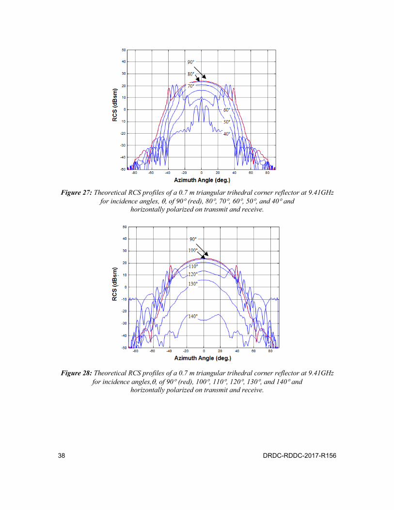
38 DRDC-RDDC-2017-R156
Figure 27: Theoretical RCS profiles of a 0.7 m triangular trihedral corner reflector at 9.41GHz
for incidence angles, , of 90 (red), 80, 70, 60, 50, and 40 and horizontally polarized on transmit and receive.
Figure 28: Theoretical RCS profiles of a 0.7 m triangular trihedral corner reflector at 9.41GHz
for incidence angles,, of 90 (red), 100, 110, 120, 130, and 140 and horizontally polarized on transmit and receive.

DRDC-RDDC-2017-R156 39
Figure 29: Theoretical RCS profiles of a 0.7 m triangular trihedral corner reflector at 9.41GHz
for incidence angles, , of 90 (red), 800, 70, 60, 50, and 40 and vertically polarized on transmit and receive.
Figure 30: Theoretical RCS profiles of a 0.7 m triangular trihedral corner reflector at 9.41GHz
for incidence angles,, of 90 (red), 100, 110, 120, 130, and 140 and vertically polarized on transmit and receive.
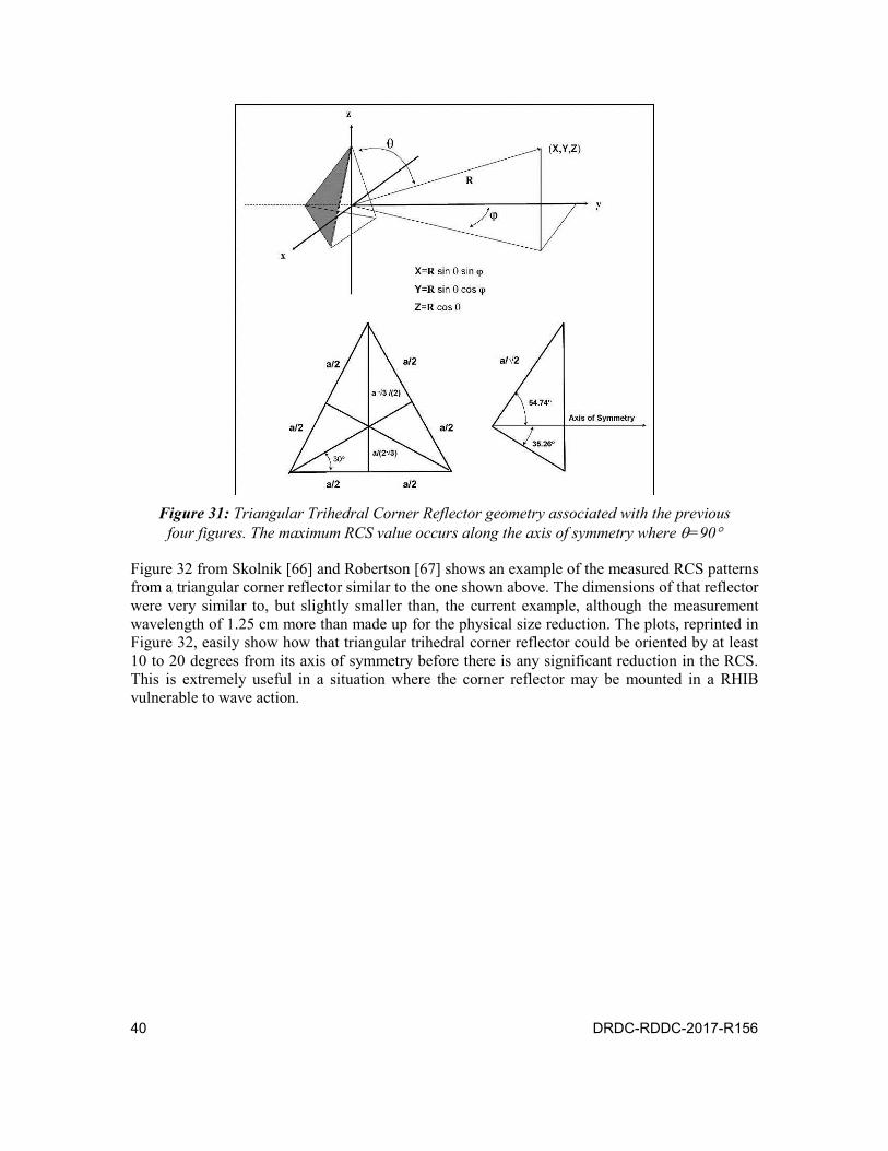
40 DRDC-RDDC-2017-R156
Figure 31: Triangular Trihedral Corner Reflector geometry associated with the previous
four figures. The maximum RCS value occurs along the axis of symmetry where =90
Figure 32 from Skolnik [66] and Robertson [67] shows an example of the measured RCS patterns from a triangular corner reflector similar to the one shown above. The dimensions of that reflector were very similar to, but slightly smaller than, the current example, although the measurement wavelength of 1.25 cm more than made up for the physical size reduction. The plots, reprinted in Figure 32, easily show how that triangular trihedral corner reflector could be oriented by at least 10 to 20 degrees from its axis of symmetry before there is any significant reduction in the RCS. This is extremely useful in a situation where the corner reflector may be mounted in a RHIB vulnerable to wave action.
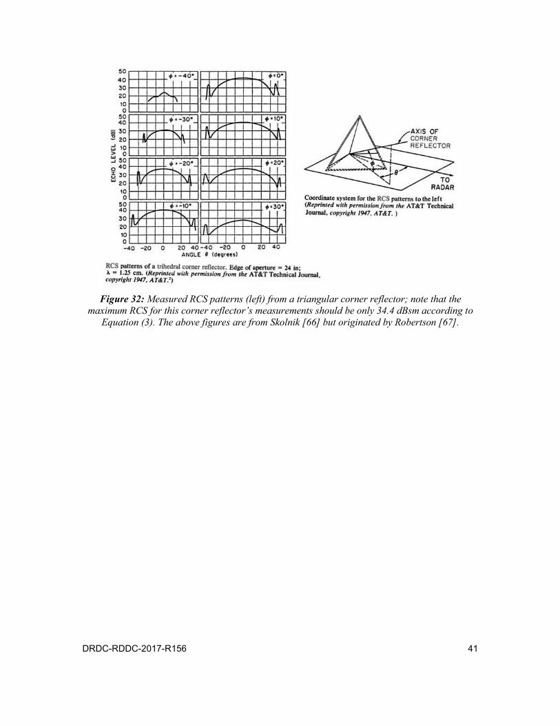
DRDC-RDDC-2017-R156 41
Figure 32: Measured RCS patterns (left) from a triangular corner reflector; note that the
maximum RCS for this corner reflector’s measurements should be only 34.4 dBsm according to Equation (3). The above figures are from Skolnik [66] but originated by Robertson [67].

42 DRDC-RDDC-2017-R156
5 SIESTA Radar Performance Prediction for NESTRA
The RF SIESTA software was used to generate a number of radar coverage plots (i.e., two dimensional Constant Altitude Plan Position Indicator (CAPPI) plots) to predict the performance and coverage areas of the Rutter 100S6 radar system in detecting different maritime targets under various environmental conditions. The analysis was based on the specifications of the Sperry BridgeMaster E transceiver and eight foot antenna that were used as the Rutter system’s front-end, combined with the use of Canadian Digital Elevation Data (CDED, scale 1:250000) with a resolution of 1 m vertically and 100 m grid spacing horizontally. Each coverage plot predicts the minimum detectable RCS of a target as a function of range, azimuth and environmental conditions (including terrain effects) for a given sensor location and target height (i.e., “constant altitude”). The different environmental conditions considered were: sea-state (SS), rain rate (mm/hr), wind direction (wd) relative to true North (°T), and wind-speed (ws). Although an exhaustive evaluation was not carried out, the plots provided in this section were representative of different times over the full trials period.
Figure 33 shows a comparison sequence of such plots, assuming a distributed target with a height of up to 20 m ASL and the radar antenna at an altitude of 27 m ASL. The sequence corresponds to sea-states between 1 and 4 (SS1 to SS4), precipitation rates of 1, 2 and 10 mm/h, wind-speeds of up to 10.9 m/s.
Figures 34 to 37 show SIESTA CAPPI plots corresponding to different environmental conditions for point, and distributed targets of 2 m ASL and 20 m ASL respectively. The right side of each figure also shows the expected minimum detectable RCS along a single radial direction from the radar site (e.g., 140° T) along with the expected maximum detection range of a small and large vessel (i.e., Quest) relative to the LOS range to the horizon.
Although not presented in this report, a more detailed and exhaustive set of predictions can be made based on the radar to target geometries, higher resolution terrain models (e.g., CDED scale 1:50000) and more detailed environmental data collected from local environmental sensors and Environment Canada weather models. Included in the following section on data collection and analysis is a brief overview of some of the weather data that was collected during the trials, and what the sources were. Also included are some photographs of the rapidly changing weather conditions from day-to-day.

DRDC-RDDC-2017-R156 43
Figure 33: SIESTA radar coverage predictions plots (minimum detectable RCS) for NESTRA
based on an antenna at an altitude of 27 m ASL and assuming a distributed target height of up to 20 m ASL.

44 DRDC-RDDC-2017-R156
Figure 34: Predicted radar coverage for a 27 m ASL antenna and a point target of 2 m ASL,
at SS1 with no precipitation. The plot to the left is a corresponding slice along a bearing radial of 140.
Figure 35: Predicted radar coverage as in Figure 34 but assuming a distributed target (not a point source) up to 2 m ASL. The predicted maximum range to detect a small vessel of 10 to
15 dBsm is 14 to 16 km. The maximum detectable range of a 75 dBsm target is 31.4 km.
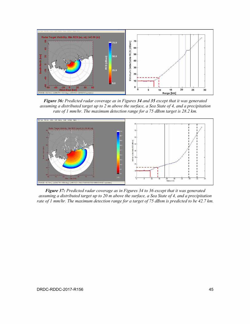
DRDC-RDDC-2017-R156 45
Figure 36: Predicted radar coverage as in Figures 34 and 35 except that it was generated
assuming a distributed target up to 2 m above the surface, a Sea State of 4, and a precipitation rate of 1 mm/hr. The maximum detection range for a 75 dBsm target is 28.2 km.
Figure 37: Predicted radar coverage as in Figures 34 to 36 except that it was generated
assuming a distributed target up to 20 m above the surface, a Sea State of 4, and a precipitation rate of 1 mm/hr. The maximum detection range for a target of 75 dBsm is predicted to be 42.7 km.

46 DRDC-RDDC-2017-R156
6 Data Collection and Analysis
6.1 Results
6.1.1 Environmental Data
During the Trials, a number of different sources of environmental data were collected with the goal of using the information to help characterize the performance of the sensors, and to predict their future capabilities. The sources of environmental data included the following:
1. HPAC data: the name is an acronym derived from Hazard Prediction and Assessment Capability for Chemical, Biological, Radiological and Nuclear (CBRN) prediction of fallout patterns, growth patterns etc. However, it is also useful for propagation prediction because it consists of a geographic grid of vertical profiles for temperature, pressure, humidity and wind velocity generated from high fidelity weather models. This data was published daily on a website set up by Dr. Forand in cooperation with DND’s Directorate of Meteorology and Oceanography (DMetOc).
2. Buoy data: Buoys located in the NESTRA AOR provided temporal information on tides, and wave characteristics such as wave height, and wave spectrum. They also provided other standard atmospheric parameters such as wind speed, wind direction, atmospheric pressure, and temperature at, or near, sea level. One such buoy was designated as Buoy 44258, which, coincidentally was one of the buoys used as a landmark to orient the radar display during post processing. This buoy is owned, maintained and used by Environment Canada, but is also used by the (U.S.) National Oceanographic and Atmospheric Administration’s (NOAA) National Data Buoy Center (NDBC) as an important source of real-time environmental data.
3. Valcartier Meteorological sensors (Vaisala probes) (see Figure 22).
4. Environment Canada Archives-National Climate Data and Information Archive (www.climate.weatheroffice.ec.gc.ca/climateData/canada_e.html) maintains an archival database of weather information of varying fidelity (temporal and parametric) from points at, and around, the NESTRA site (see Figure 38), such as:
a. Osborne Head DND (a.k.a. NESTRA): 44 36.767’N, 63 25.383’W, Altitude=30 m
b. Shearwater A (airport): 44 38.0’ N, 63 30.0’ W, Altitude=50.9 m
c. Shearwater Jetty: 44 37.67’ N, 63 31.4’ W, Altitude=5.50 m
d. Shearwater Auto: 44 38.18’ N, 63 30.4’ W, Altitude=53 m
e. Shearwater RCS: 44 37.78’ N, 63 30.8’ W, Altitude=24 m
f. Halifax Dockyard: 44 39.32’ N, 63 34.6’ W, Altitude=3.0 m

DRDC-RDDC-2017-R156 47
Figure 38: Locations of six weather stations (indicated by cloud/rain symbols), in and around
Halifax, that contribute to Environment Canada’s archival database.
The weather conditions varied greatly over the course of the trials period, covering a spectrum of conditions similar to those experienced by the author in the Arctic during field trials earlier in August 2008. The NESTRA conditions for the Trials period are summarized by Figure 39 and Figure 40 and in Table 6. However, the information in Table 6 does not cover the entire 24 hour period of each day because the information was recorded manually, and the airfield was typically only open between 06:00 and 19:00 each day. Further evidence of the weather conditions is indicated by the scene variation evident in the photographs taken by the author throughout the trials period, specifically Figure 21 to Figure 24, and Figure 41 to Figure 51.

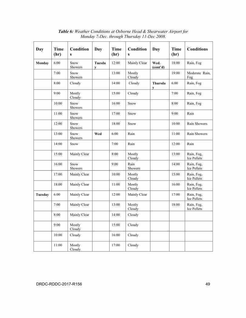
DRDC-RDDC-2017-R156 49
Table 6: Weather Conditions at Osborne Head & Shearwater Airport for Monday 7-Dec. through Thursday 11-Dec 2008.
Day Time (hr)
Conditions
Day Time (hr)
Conditions
Day Time (hr)
Conditions
Monday 6:00 Snow Showers
Tuesday (cont’d)
12:00 Mainly Clear Wed. (cont’d)
18:00 Rain, Fog
7:00 Snow Showers
13:00 Mostly Cloudy
19:00 Moderate Rain, Fog
8:00 Cloudy 14:00 Cloudy Thursday
6:00 Rain, Fog
9:00 Mostly Cloudy
15:00 Cloudy 7:00 Rain, Fog
10:00 Snow Showers
16:00 Snow 8:00 Rain, Fog
11:00 Snow Showers
17:00 Snow 9:00 Rain
12:00 Snow Showers
18:00 Snow 10:00 Rain Showers
13:00 Snow Showers
Wed 6:00 Rain 11:00 Rain Showers
14:00 Snow 7:00 Rain 12:00 Rain
15:00 Mainly Clear 8:00 Mostly Cloudy
13:00 Rain, Fog, Ice Pellets
16:00 Snow Showers
9:00 Rain Showers
14:00 Rain, Fog, Ice Pellets
17:00 Mainly Clear 10:00 Mostly Cloudy
15:00 Rain, Fog, Ice Pellets
18:00 Mainly Clear 11:00 Mostly Cloudy
16:00 Rain, Fog, Ice Pellets
Tuesday 6:00 Mainly Clear 12:00 Mainly Clear 17:00 Rain, Fog, Ice Pellets
7:00 Mainly Clear 13:00 Mostly Cloudy
18:00 Rain, Fog, Ice Pellets
8:00 Mainly Clear 14:00 Cloudy
9:00 Mostly Cloudy
15:00 Cloudy
10:00 Cloudy 16:00 Cloudy
11:00 Mostly Cloudy
17:00 Cloudy

50 DRDC-RDDC-2017-R156
Figure 41: Stitched panorama from pictures taken at 7:55 am Monday morning at NESTRA.
Figure 42: High surf directly east of Osborne Head (NESTRA) at approximately 8:00 am on
Monday morning (photo by the author).
Figure 43: Photos by the author showing the wind-blown surf just east of NESTRA (top left) and
about 3 km south of NESTRA (top right, and bottom), just east of Hartlen Point. These can be compared to the photos in Figure 20.

DRDC-RDDC-2017-R156 51
Figure 44: View looking east from NESTRA at 1:18 pm on Monday showing the surf due to the
high winds; the CFAV Quest can also be seen in the centre of the photo with an expanded view shown in the inset (photo by the author).
Figure 45: Photo of the AWS with the main NESTRA building in the background; taken at
4:21 pm Monday afternoon (courtesy of Dr. V. Larochelle).

52 DRDC-RDDC-2017-R156
Figure 46: RHIB approaching the Quest after the calibration run on
Tuesday afternoon, 9 Dec. 2008.
Figure 47: Photo taken by the author looking eastward from NESTRA on Tuesday morning,
9 Dec. 2008. The inset is a blow-up of the CFAV Quest (on the left) and a freighter (Atlantic Superior) heading to Halifax Harbour.

DRDC-RDDC-2017-R156 53
Figure 48: Photo by the author taken on the calmest day of the trials, Tues. 9 Dec. 2008.
The inset shows the Quest and a smaller fishing vessel to its right.
Figure 49: Photo by the author taken at 11:23 local time, Tues. 9 Dec. 2008. The inset
on the right shows a blow-up of the Quest, and the one on the left shows a couple of the local fishing vessels.
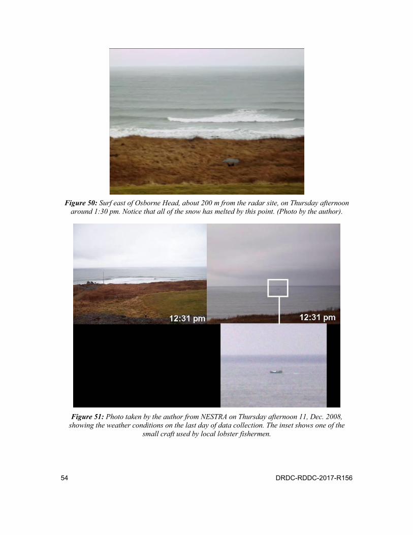
54 DRDC-RDDC-2017-R156
Figure 50: Surf east of Osborne Head, about 200 m from the radar site, on Thursday afternoon
around 1:30 pm. Notice that all of the snow has melted by this point. (Photo by the author).
Figure 51: Photo taken by the author from NESTRA on Thursday afternoon 11, Dec. 2008,
showing the weather conditions on the last day of data collection. The inset shows one of the small craft used by local lobster fishermen.
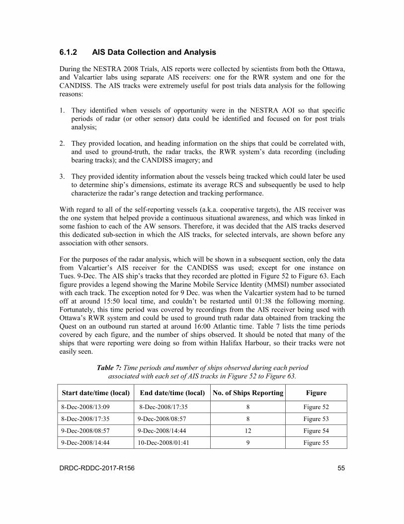
DRDC-RDDC-2017-R156 55
6.1.2 AIS Data Collection and Analysis
During the NESTRA 2008 Trials, AIS reports were collected by scientists from both the Ottawa, and Valcartier labs using separate AIS receivers: one for the RWR system and one for the CANDISS. The AIS tracks were extremely useful for post trials data analysis for the following reasons:
1. They identified when vessels of opportunity were in the NESTRA AOI so that specific periods of radar (or other sensor) data could be identified and focused on for post trials analysis;
2. They provided location, and heading information on the ships that could be correlated with, and used to ground-truth, the radar tracks, the RWR system’s data recording (including bearing tracks); and the CANDISS imagery; and
3. They provided identity information about the vessels being tracked which could later be used to determine ship’s dimensions, estimate its average RCS and subsequently be used to help characterize the radar’s range detection and tracking performance.
With regard to all of the self-reporting vessels (a.k.a. cooperative targets), the AIS receiver was the one system that helped provide a continuous situational awareness, and which was linked in some fashion to each of the AW sensors. Therefore, it was decided that the AIS tracks deserved this dedicated sub-section in which the AIS tracks, for selected intervals, are shown before any association with other sensors.
For the purposes of the radar analysis, which will be shown in a subsequent section, only the data from Valcartier’s AIS receiver for the CANDISS was used; except for one instance on Tues. 9-Dec. The AIS ship’s tracks that they recorded are plotted in Figure 52 to Figure 63. Each figure provides a legend showing the Marine Mobile Service Identity (MMSI) number associated with each track. The exception noted for 9 Dec. was when the Valcartier system had to be turned off at around 15:50 local time, and couldn’t be restarted until 01:38 the following morning. Fortunately, this time period was covered by recordings from the AIS receiver being used with Ottawa’s RWR system and could be used to ground truth radar data obtained from tracking the Quest on an outbound run started at around 16:00 Atlantic time. Table 7 lists the time periods covered by each figure, and the number of ships observed. It should be noted that many of the ships that were reporting were doing so from within Halifax Harbour, so their tracks were not easily seen.
Table 7: Time periods and number of ships observed during each period associated with each set of AIS tracks in Figure 52 to Figure 63.
Start date/time (local) End date/time (local) No. of Ships Reporting Figure
8-Dec-2008/13:09 8-Dec-2008/17:35 8 Figure 52
8-Dec-2008/17:35 9-Dec-2008/08:57 8 Figure 53
9-Dec-2008/08:57 9-Dec-2008/14:44 12 Figure 54
9-Dec-2008/14:44 10-Dec-2008/01:41 9 Figure 55
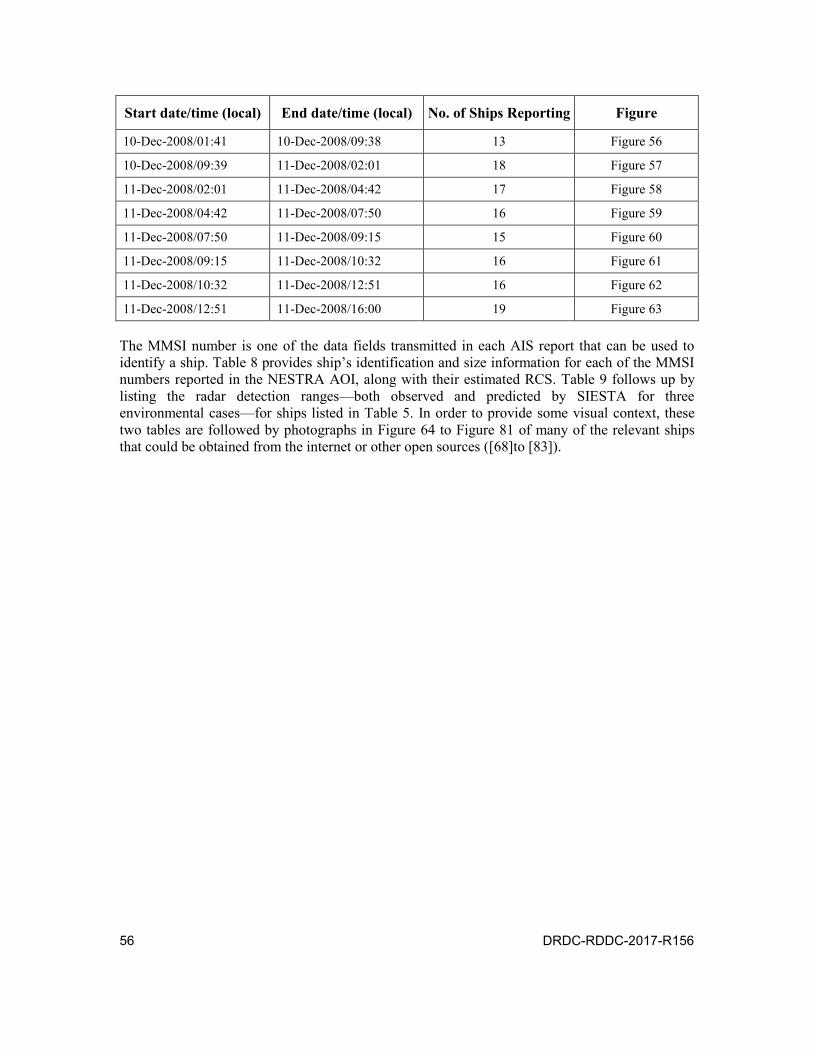
56 DRDC-RDDC-2017-R156
Start date/time (local) End date/time (local) No. of Ships Reporting Figure
10-Dec-2008/01:41 10-Dec-2008/09:38 13 Figure 56
10-Dec-2008/09:39 11-Dec-2008/02:01 18 Figure 57
11-Dec-2008/02:01 11-Dec-2008/04:42 17 Figure 58
11-Dec-2008/04:42 11-Dec-2008/07:50 16 Figure 59
11-Dec-2008/07:50 11-Dec-2008/09:15 15 Figure 60
11-Dec-2008/09:15 11-Dec-2008/10:32 16 Figure 61
11-Dec-2008/10:32 11-Dec-2008/12:51 16 Figure 62
11-Dec-2008/12:51 11-Dec-2008/16:00 19 Figure 63
The MMSI number is one of the data fields transmitted in each AIS report that can be used to identify a ship. Table 8 provides ship’s identification and size information for each of the MMSI numbers reported in the NESTRA AOI, along with their estimated RCS. Table 9 follows up by listing the radar detection ranges—both observed and predicted by SIESTA for three environmental cases—for ships listed in Table 5. In order to provide some visual context, these two tables are followed by photographs in Figure 64 to Figure 81 of many of the relevant ships that could be obtained from the internet or other open sources ([68]to [83]).

DRDC-RDDC-2017-R156 57
Figure 52: Valcartier AIS tracks; the legend displays the MMSI number associated with each
ship track during the period from 13:09 to 17:35 on Monday Dec. 8.
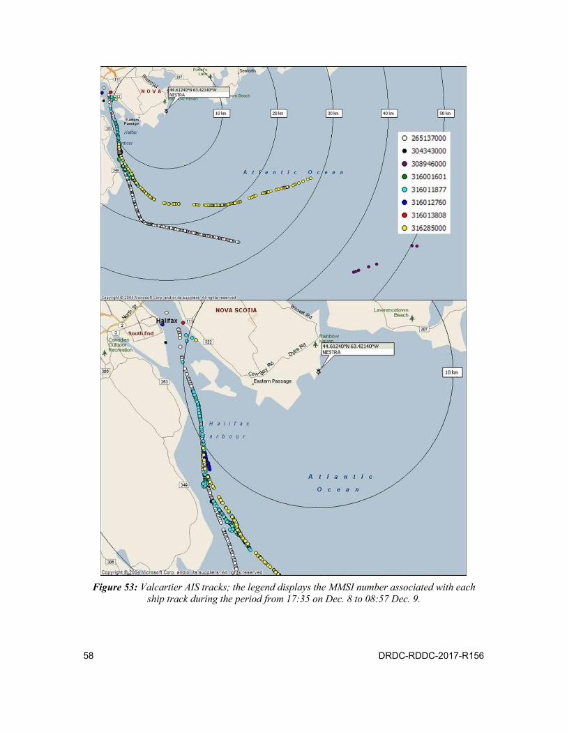
58 DRDC-RDDC-2017-R156
Figure 53: Valcartier AIS tracks; the legend displays the MMSI number associated with each
ship track during the period from 17:35 on Dec. 8 to 08:57 Dec. 9.

DRDC-RDDC-2017-R156 59
Figure 54: Valcartier AIS tracks including Quest with manoeuvres; the legend displays the MMSI
number associated with each ship track during the period from 08:57 to 14:44 on Dec. 9.

60 DRDC-RDDC-2017-R156
Figure 55: Valcartier AIS tracks; the legend displays the MMSI number associated with each
ship track during the period from 14:44 on Dec. 9 to 01:41 on Dec. 10.
Figure 56: Valcartier AIS tracks; the legend displays the MMSI number associated with each
ship track during the period from 01:41 to 09:38 on Dec. 10.

DRDC-RDDC-2017-R156 61
Figure 57: AIS tracks; the legend displays the MMSI number associated with each ship track
during the period from 09:39 on Dec. 10 to 02:01 on Dec. 11.

62 DRDC-RDDC-2017-R156
Figure 58: AIS tracks; the legend displays the MMSI number associated with each ship track
during the period from 02:01 to 04:42 on Dec. 11.
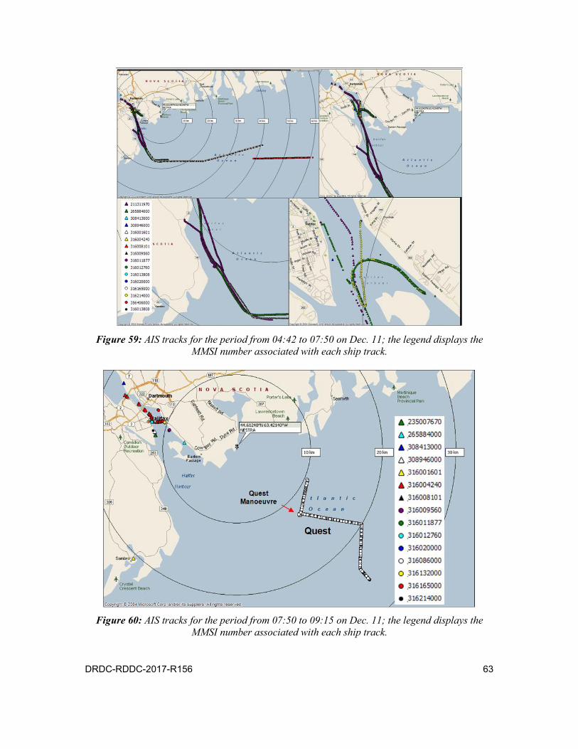
DRDC-RDDC-2017-R156 63
Figure 59: AIS tracks for the period from 04:42 to 07:50 on Dec. 11; the legend displays the
MMSI number associated with each ship track.
Figure 60: AIS tracks for the period from 07:50 to 09:15 on Dec. 11; the legend displays the
MMSI number associated with each ship track.

64 DRDC-RDDC-2017-R156
Figure 61: AIS tracks for the period from 09:15 to 10:32 on Dec. 11; the legend displays the
MMSI number associated with each ship track.

DRDC-RDDC-2017-R156 65
Figure 62: AIS tracks for the period from 10:32 to 12:51 on Dec. 11; the legend displays the
MMSI number associated with each ship track.
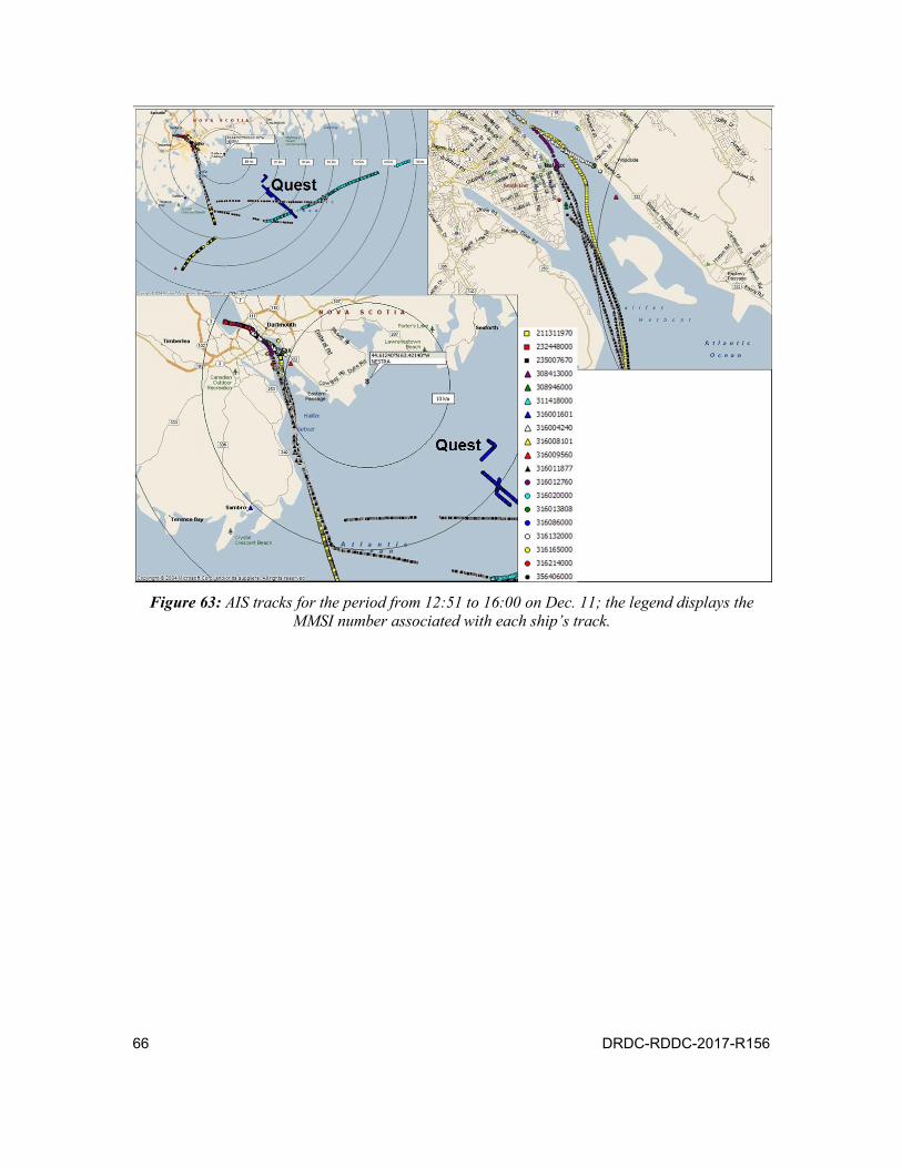
66 DRDC-RDDC-2017-R156
Figure 63: AIS tracks for the period from 12:51 to 16:00 on Dec. 11; the legend displays the
MMSI number associated with each ship’s track.

DRDC-RDDC-2017-R156 67
Table 8: List of ships tracked by AIS in the NESTRA AOI during the AWS trials; the dimensions of each ship—identified by MMSI#, call-sign, and ship’s name—are provided, along with their
gross tonnage and, where possible, their RCS estimates based on Equation (2).
MMSI # Call Sign
Ship’s Name Length (m)
Width (m)
Stack Ht/ Bridge Ht/ Deck Ht
(m)
Gross tons
RCS Estimate
dBsm
211311970 DGAF Antwerp Express 295 32 37.8/33.6/10.3 67145 41 to 57
232448000 MHNL6 British Courtesy 184 32 31.4/26.9/12 29214 38 to 53
235007670 MFAU5 Zim Pusan 292 32 42.3/37.9/10.5 62740 40 to 57
265137000 SKOZ Atlantic Concert 292 31 36.8/32.8/15.2 57255 40 to 57
265884000 SHJC Undine 228 32 33.5/33.5/22.9 28388 37 to 53
304343000 V2009 Nirint Force 134 20 35.6/30.0/6.1 8861 33 to 47
308413000 C6VE6 Atlantic Superior 222 23 28.0/26.0/8.6 38510 39 to 55
308946000 C6WI6 Skandi Bergen 106 22 31.3/24.1/3.2 6596 32 to 44
311418000 C6SP2 Rega 149 24 16880 36 to 50
316001601 CG 2613 CCGC SAMBRO 16 9.6/5.1/1.6 36 13 to 19
316004240 CFH8945 Atlantic Oak 31 11 15.4/8.2/2.7 402 22 to 31
316008101 n/a APA No. 20 20 5 8.7/4.4/1.0
316009560 VAAP Algoscotia 148.8 23.8 23.7/23.7/8.3 13352 35 to 49
316011877 VC9066 APA No. 1 20 5 11.2/6.0/2.3
316012760 XJAG Svitzerbedford 29 10.5 11.6/9.0/3.0 370 22 to 31
316013808 CFH8990 Atlantic Bear 28.8 12 15.4/8.2/2.7 399 22 to 31
316020000 n/g CCGS Edward Cornwallis
83 16.2 19.5/14.3/6.2 3727 30 to 42
316053000 CGUM CCGS Sir William Alexander
83 16.2 19.5/14.3/6.2 3727 30 to 42
316086000 CZDO CFAV Quest 76 12.6 21.1/13.0/5.2 2130 28 to 40
316132000 VORM Hebron Sea 78 16 15.4/14.4/6.3 1374 26 to 37
316165000 CGBN CCGS Louis S. St Laurent
120 24 28.8/18.6/9.3 11345 34 to 48
316214000 VCRT Kometik 261 46 39.3/33.3/14.4 76216 41 to 58
316285000 VCWL Maria Desgagnes 114 21 23.3/21.9/6.7 14335 35 to 50
356406000 3ELV3 Sirius Highway 172 32 34.7/35.5/29.4 44576 39 to 55
477806000 VRWN4 OOCL San Francisco
227 40 38.0/31.4/11.5 67286 41 to 57
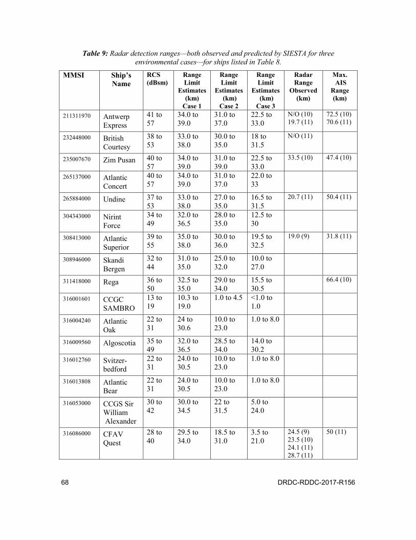
68 DRDC-RDDC-2017-R156
Table 9: Radar detection ranges—both observed and predicted by SIESTA for three environmental cases—for ships listed in Table 8.
MMSI Ship’s Name
RCS (dBsm)
Range Limit
Estimates (km)
Case 1
Range Limit
Estimates (km)
Case 2
Range Limit
Estimates (km)
Case 3
Radar Range
Observed (km)
Max. AIS
Range (km)
211311970 Antwerp Express
41 to 57
34.0 to 39.0
31.0 to 37.0
22.5 to 33.0
N/O (10) 19.7 (11)
72.5 (10) 70.6 (11)
232448000 British Courtesy
38 to 53
33.0 to 38.0
30.0 to 35.0
18 to 31.5
N/O (11)
235007670 Zim Pusan 40 to 57
34.0 to 39.0
31.0 to 39.0
22.5 to 33.0
33.5 (10) 47.4 (10)
265137000 Atlantic Concert
40 to 57
34.0 to 39.0
31.0 to 37.0
22.0 to 33
265884000 Undine 37 to 53
33.0 to 38.0
27.0 to 35.0
16.5 to 31.5
20.7 (11) 50.4 (11)
304343000 Nirint Force
34 to 49
32.0 to 36.5
28.0 to 35.0
12.5 to 30
308413000 Atlantic Superior
39 to 55
35.0 to 38.0
30.0 to 36.0
19.5 to 32.5
19.0 (9) 31.8 (11)
308946000 Skandi Bergen
32 to 44
31.0 to 35.0
25.0 to 32.0
10.0 to 27.0
311418000 Rega 36 to 50
32.5 to 35.0
29.0 to 34.0
15.5 to 30.5
66.4 (10)
316001601 CCGC SAMBRO
13 to 19
10.3 to 19.0
1.0 to 4.5 <1.0 to 1.0
316004240 Atlantic Oak
22 to 31
24 to 30.6
10.0 to 23.0
1.0 to 8.0
316009560 Algoscotia 35 to 49
32.0 to 36.5
28.5 to 34.0
14.0 to 30.2
316012760 Svitzer-bedford
22 to 31
24.0 to 30.5
10.0 to 23.0
1.0 to 8.0
316013808 Atlantic Bear
22 to 31
24.0 to 30.5
10.0 to 23.0
1.0 to 8.0
316053000 CCGS Sir William Alexander
30 to 42
30.0 to 34.5
22 to 31.5
5.0 to 24.0
316086000 CFAV Quest
28 to 40
29.5 to 34.0
18.5 to 31.0
3.5 to 21.0
24.5 (9) 23.5 (10) 24.1 (11) 28.7 (11)
50 (11)
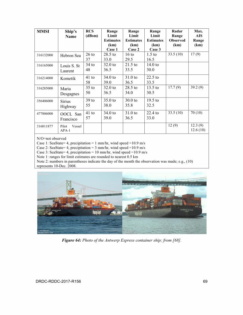
DRDC-RDDC-2017-R156 69
MMSI Ship’s Name
RCS (dBsm)
Range Limit
Estimates (km)
Case 1
Range Limit
Estimates (km)
Case 2
Range Limit
Estimates (km)
Case 3
Radar Range
Observed (km)
Max. AIS
Range (km)
316132000 Hebron Sea 26 to 37
28.5 to 33.0
16 to 29.5
1.5 to 16.5
33.5 (10) 17 (9)
316165000 Louis S. St Laurent
34 to 48
32.0 to 36.5
21.5 to 33.5
14.0 to 30.0
316214000 Kometik 41 to 58
34.0 to 39.0
31.0 to 36.5
22.5 to 33.5
316285000 Maria Desgagnes
35 to 50
32.0 to 36.5
28.5 to 34.0
13.5 to 30.5
17.7 (9) 39.2 (9)
356406000 Sirius Highway
39 to 55
35.0 to 38.0
30.0 to 35.8
19.5 to 32.5
477806000 OOCL San Francisco
41 to 57
34.0 to 39.0
31.0 to 36.5
22.4 to 33.0
33.5 (10) 70 (10)
316011877 Pilot Vessel APA-1
12 (9) 12.3 (9) 12.6 (10)
N/O=not observed Case 1: SeaState= 4, precipitation = 1 mm/hr, wind speed =10.9 m/s Case 2: SeaState= 4, precipitation = 3 mm/hr, wind speed =10.9 m/s Case 3: SeaState= 4, precipitation = 10 mm/hr, wind speed =10.9 m/s Note 1: ranges for limit estimates are rounded to nearest 0.5 km Note 2: numbers in parentheses indicate the day of the month the observation was made; e.g., (10) represents 10-Dec. 2008.
Figure 64: Photo of the Antwerp Express container ship; from [68].

70 DRDC-RDDC-2017-R156
Figure 65: Sir William Alexander, Canadian Coast Guard Ship (CCGS) ice-breaker; from [69].
Figure 66: Photographs of the CCGS Louis St. Laurent from the CCG web-site [69].
Figure 67: Photos of Skandi Bergen; from [70].
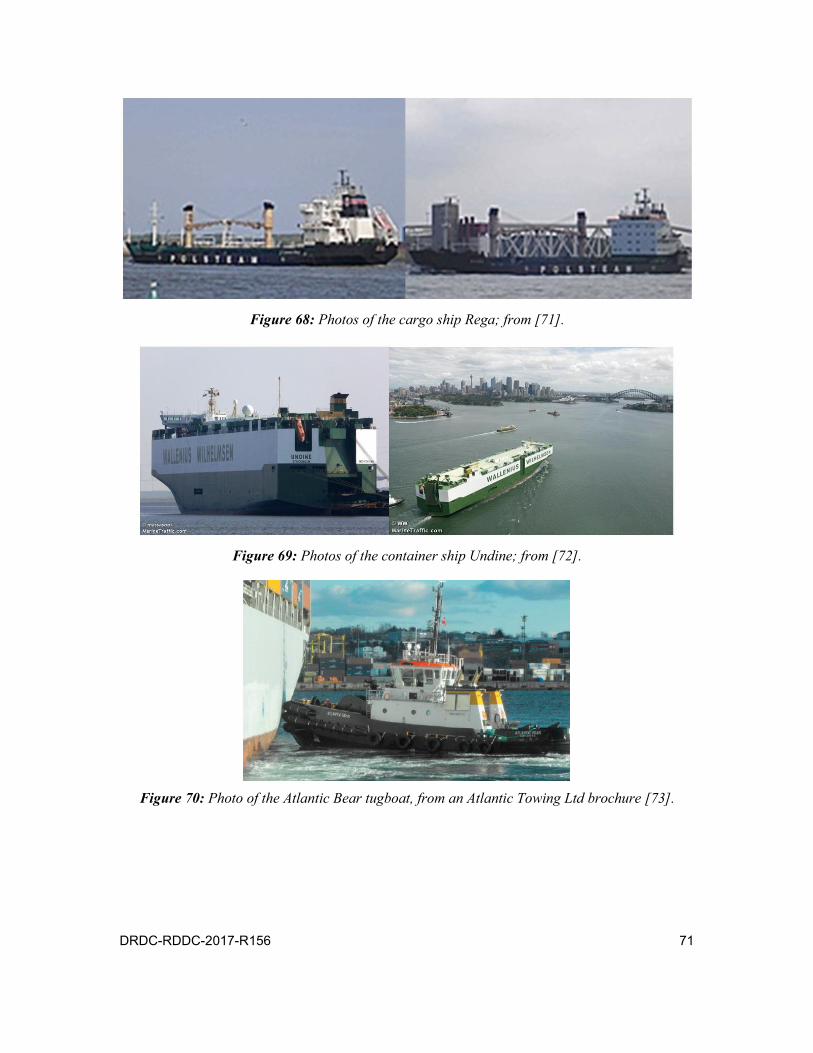
DRDC-RDDC-2017-R156 71
Figure 68: Photos of the cargo ship Rega; from [71].
Figure 69: Photos of the container ship Undine; from [72].
Figure 70: Photo of the Atlantic Bear tugboat, from an Atlantic Towing Ltd brochure [73].

72 DRDC-RDDC-2017-R156
Figure 71: Photos of the OOCL San Francisco, container ship; from [74].
Figure 72: Photos of the cargo/container ship Sirius Highway; from [75].
Figure 73: Photo of the container ship Atlantic Concert; (photo by the author, 20 Oct. 2005).

DRDC-RDDC-2017-R156 73
Figure 74: Photos of the container ship Zim Pusan; from [76] (Photo by K. Watson).
Figure 75: Photographs of the cargo ship British Courtesy; from [77]
(Left photo by D. Kannengießer).
Figure 76: Photos of the tanker ship Maria Desgagnes; from [78].

74 DRDC-RDDC-2017-R156
Figure 77: Photo of the container ship Atlantic Superior; from [79] (Photo by K. Watson).
Figure 78: A photograph of the Nirint Force, a container vessel in the Halifax area during the
NESTRA Trials; from [80] (Photo by M. Schindler).
Figure 79: Photograph of the tug Svitzer Bedford (Photo by M. MacKay [81]).
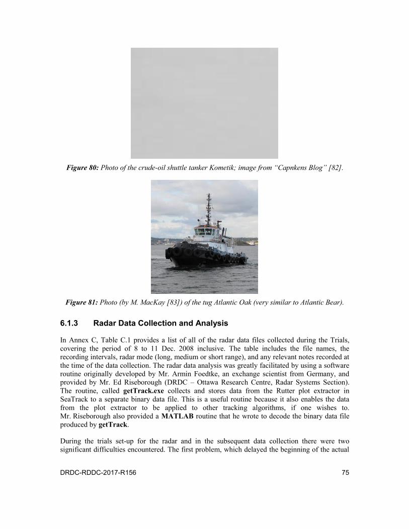
DRDC-RDDC-2017-R156 75
Figure 80: Photo of the crude-oil shuttle tanker Kometik; image from “Capnkens Blog” [82].
Figure 81: Photo (by M. MacKay [83]) of the tug Atlantic Oak (very similar to Atlantic Bear).
6.1.3 Radar Data Collection and Analysis
In Annex C, Table C.1 provides a list of all of the radar data files collected during the Trials, covering the period of 8 to 11 Dec. 2008 inclusive. The table includes the file names, the recording intervals, radar mode (long, medium or short range), and any relevant notes recorded at the time of the data collection. The radar data analysis was greatly facilitated by using a software routine originally developed by Mr. Armin Foedtke, an exchange scientist from Germany, and provided by Mr. Ed Riseborough (DRDC – Ottawa Research Centre, Radar Systems Section). The routine, called getTrack.exe collects and stores data from the Rutter plot extractor in SeaTrack to a separate binary data file. This is a useful routine because it also enables the data from the plot extractor to be applied to other tracking algorithms, if one wishes to. Mr. Riseborough also provided a MATLAB routine that he wrote to decode the binary data file produced by getTrack.
During the trials set-up for the radar and in the subsequent data collection there were two significant difficulties encountered. The first problem, which delayed the beginning of the actual

76 DRDC-RDDC-2017-R156
data collection until the latter portion of the Dec. 8, appeared to be a problem with communication between the radar transceiver and the back-end processor. The result was that the radar PPI display could not be generated by the computer on the SeaView GUI. After some systems troubleshooting, it was discovered that there may have been a problem with the “seating” of the Sigma 6 processor card in the host computer as a result of vibration during shipping. This was finally fixed by opening the computer chassis and re-seating the card on the PC motherboard.
The second, more subtle, difficulty that was encountered during the data analysis stemmed from an incorrect procedure in the original data collection which was due to insufficient familiarity with the system (one of the reasons for these shake-down trials). As part of the data collection procedure, it had been decided from the onset that data files should be kept to a reasonable size, to facilitate archiving, and data exchange. Therefore data collection periods tended to be less than one hour in length with the subsequent file sizes usually less than 10 GB and often less than 4 GB. In an attempt to improve the speed and efficiency of the radar data collection, and to minimize the loss of radar data between successive files, a number of pre-named “empty” files were created in advance, then “selected” at the start of a new data acquisition run. The confusion (and problems) occurred because there are two different routines controlling separate aspects of the data collection process that require a start/stop control for each new data file. Under normal procedures, the SeaScan Server software must be activated first, and a default file selected for recording or playing back data (see Figure 82). However, it was learned later that for each new data run, the SeaScan Server software must be stopped and then restarted for each new data file. According to Section 4.2.3 of the SeaScan Technical Manual [84] for recording data to a disk:
“The system records to ARCHIVE.DAT in the current directory... Currently the server does not support changing data files. If it is necessary to record to a different file, the server must be stopped and ARCHIVE.DAT renamed as appropriate.”
In practice it is actually less restrictive to name files than is implied by the above statement, because the default file to which one will record the data can have any name as long as it doesn’t exceed a maximum length and doesn’t contain special characters. However, to correctly log raw radar data without corruption, the SeaScan routine must first be stopped, and then restarted, followed by selecting a new data file as the default before initiating data collection to the new data file. This problem may be corrected in subsequent releases of the radar software suite.

DRDC-RDDC-2017-R156 77
Figure 82: SeaScan Server software GUI to select a default data file for raw data collection or
playback prior to starting the data logging using SeaView.
While a few of the raw radar data files were collected in the correct manner, the majority had corrupted header information associated with the time stamps on the data. This made subsequent playback using the most recent version of SeaView (supplied with the radar) impossible. However, for analysing the corrupted files a work-around was identified, with the help of Mr. Ed Riseborough, whereby an earlier version of SeaView could be used to post-process the data. This work-around was used to analyse some of the files while some of the more important ones were sent to Rutter to fix the corrupted sections and return the corrected data. For reasons that are too lengthy to explain here, the work-around was not perfect because in some cases it only allowed about a third to a half of the data to be accessed and processed. This problem was captured in the table in Annex C which lists the start and stop times of each file along with the actual playback time that could be processed. In addition to the requirement of playing back the data in an earlier version of SeaView, because some of the timing data was corrupted the getTrack.exe routine had problems associating the correct time stamp for each point from the plot extractor, despite the fact that the correct time was displayed in the SeaView GUI. A separate work-around was used to solve this problem by using the number of scans since the beginning of the data collection to estimate the time. This was compared to the time displayed in the SeaView GUI, and was never off by more than a few seconds.
It would be possible to have all of the data files corrected, but it was not deemed necessary as part of the current data analysis since enough information was available to meet the requirements.
6.1.3.1 Results of the Rutter 100S6 Radar Post Processing
As indicated earlier in Sections 2.2.1 and 3.1.1, the weather conditions during the trials were quite varied, ranging from clear visibility, with relatively low sea state (< SS 2) and no precipitation to the opposite extreme of high wind and significant amounts of precipitation in the form of rain, snow or a mixture of both.
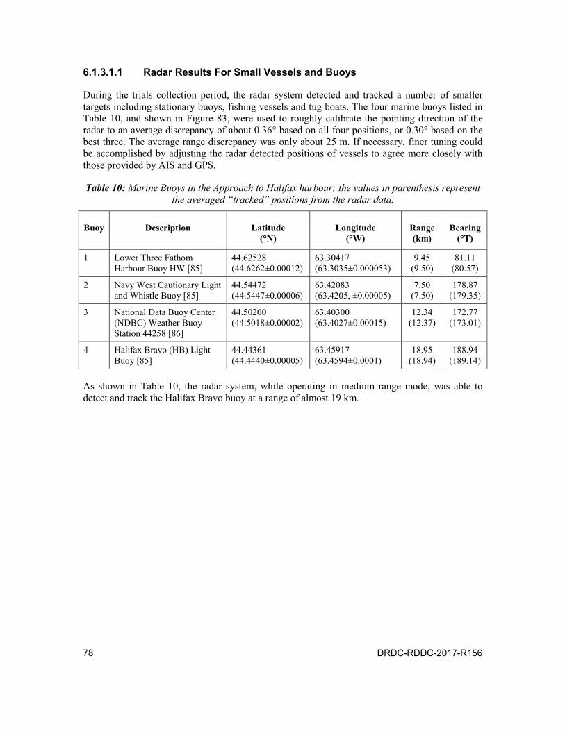
78 DRDC-RDDC-2017-R156
6.1.3.1.1 Radar Results For Small Vessels and Buoys
During the trials collection period, the radar system detected and tracked a number of smaller targets including stationary buoys, fishing vessels and tug boats. The four marine buoys listed in Table 10, and shown in Figure 83, were used to roughly calibrate the pointing direction of the radar to an average discrepancy of about 0.36° based on all four positions, or 0.30° based on the best three. The average range discrepancy was only about 25 m. If necessary, finer tuning could be accomplished by adjusting the radar detected positions of vessels to agree more closely with those provided by AIS and GPS.
Table 10: Marine Buoys in the Approach to Halifax harbour; the values in parenthesis represent the averaged “tracked” positions from the radar data.
Buoy Description Latitude (°N)
Longitude (°W)
Range (km)
Bearing (°T)
1 Lower Three Fathom Harbour Buoy HW [85]
44.62528 (44.6262±0.00012)
63.30417 (63.3035±0.000053)
9.45 (9.50)
81.11 (80.57)
2 Navy West Cautionary Light and Whistle Buoy [85]
44.54472 (44.5447±0.00006)
63.42083 (63.4205, ±0.00005)
7.50 (7.50)
178.87 (179.35)
3 National Data Buoy Center (NDBC) Weather Buoy Station 44258 [86]
44.50200 (44.5018±0.00002)
63.40300 (63.4027±0.00015)
12.34 (12.37)
172.77 (173.01)
4 Halifax Bravo (HB) Light Buoy [85]
44.44361 (44.4440±0.00005)
63.45917 (63.4594±0.0001)
18.95 (18.94)
188.94 (189.14)
As shown in Table 10, the radar system, while operating in medium range mode, was able to detect and track the Halifax Bravo buoy at a range of almost 19 km.

DRDC-RDDC-2017-R156 79
Figure 83: This chart shows the approach to Halifax harbour, including four stationary buoys
that were detected by the radar system and used to help calibrate its pointing direction. The blue circles represent the recorded positions of the buoys [85][86], and the purple flags
represent their respective radar tracks.
A radar track from the pilot tugboat, APA No. 1, while the system was operating in MR mode, is shown in Figure 84 and compared with its respective AIS track. APA No. 1 was tracked to a maximum range of 12.0 km during Sea-State 3–4 conditions when there was very little precipitation.
Figure 85 shows plotted radar tracks for a number of fishing vessels (represented by the black ellipses), the four stationary buoys (red flags) and a number of larger vessels including the Quest (coloured polygons). Although the buoy locations were known, there were no AIS tracks for the fishing vessels to correlate with the radar data to provide ground-truthed locations in order to ensure against false tracks. However, as implied by the 10 km range rings in the AOI, the fishing/lobster boats appeared to be tracked to a maximum range of between 10 km and 12 km. As implied by the accompanying photos of common fishing vessels in Figure 85 they were believed to be typically 13 to 17 m in length, and 5 to 6 m wide.

80 DRDC-RDDC-2017-R156
Figure 84: The maximum detection range for the pilot-boat APA No. 1 was 12.0 km, observed at
around 11:06 am Dec. 10 while the conditions were SS 3 to 4 with cloudy conditions but very little precipitation. (Note: the picture of APA 1 on the right, courtesy of Tim Hammond of
DRDC – Atlantic Research Centre, was taken during different set of trials.)
Of the four buoys that were detected in the AOI the farthest one (circled) was detected at 18.95 km from NESTRA. Such buoys usually carry an RCS enhancer (e.g., set of corner reflectors) to give them at least an RCS of about 10 dBsm. This provides a good estimate of the radar’s ability to detect and track a target of this size. Since they are relatively stationary, scan-to-scan averaging was also able to significantly enhance their detection.
Figure 86 to Figure 88 show some typical screen captures of the radar display while the radar was in MR mode and tracks were being collected. The screen capture of the SeaView radar display, which shows some of the echoes from the fishing/lobster vessels, is shown in Figure 86 and was generated using the more recent SeaView GUI. In contrast, the screen captures in Figure 87 and Figure 88 were generated using an earlier version of the GUI which seemed to be able to accommodate some of the radar data problems.
Figure 87 shows a SeaView radar display in MR mode while tracking the Quest’s RHIB over the period from 15:12:45 to 15:26:25 of 9 December. The RHIB remained on station at about 5.23 nmi from NESTRA and at a bearing of 115T until approximately 15:20 before returning to the Quest. The large number of plots on the screen within the auto-acquisition zone (red polygon) was because a low radar detection threshold was required to detect and track the RHIB, and as a result of maintaining the track “tails” for the entire observation period. This maintained the persistence of all detections that were promoted to “plots” or tentative tracks as well as established tracks. Figure 88 shows a screen capture of the SeaView display during a slightly earlier RHIB recording (track 202) at about 15:06; similar to Figure 87 but with a “Target Trail Length” of 0 minutes resulting in a much cleaner view.

DRDC-RDDC-2017-R156 81
Figure 85: Chart (upper left) showing plotted radar tracks for a number of fishing vessels (black
ellipses), four tethered marker buoys (red flags), and a number of larger vessels including the Quest (coloured polygons).The fishing/lobster boats were detected to a range of over 10 km.
Photos of typical vessels seen in the area under day and night conditions (extracted from CANDISS video from the trials) are shown around the periphery.

82 DRDC-RDDC-2017-R156
Figure 86: SeaView radar display (medium range mode) of mostly small boats in the NESTRA area. The display n the upper left is with
the track display on while the upper right is with it off, and the lower image is an expanded view.
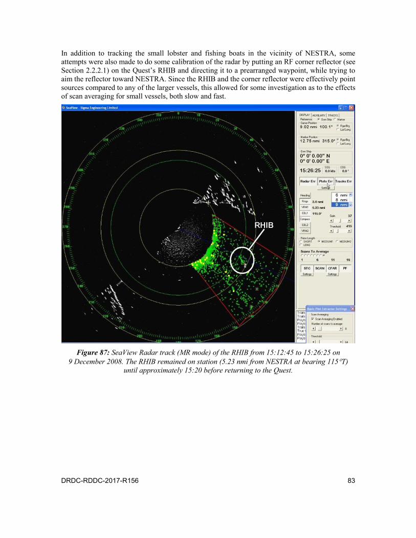
DRDC-RDDC-2017-R156 83
In addition to tracking the small lobster and fishing boats in the vicinity of NESTRA, some attempts were also made to do some calibration of the radar by putting an RF corner reflector (see Section 2.2.2.1) on the Quest’s RHIB and directing it to a prearranged waypoint, while trying to aim the reflector toward NESTRA. Since the RHIB and the corner reflector were effectively point sources compared to any of the larger vessels, this allowed for some investigation as to the effects of scan averaging for small vessels, both slow and fast.
Figure 87: SeaView Radar track (MR mode) of the RHIB from 15:12:45 to 15:26:25 on
9 December 2008. The RHIB remained on station (5.23 nmi from NESTRA at bearing 115T) until approximately 15:20 before returning to the Quest.
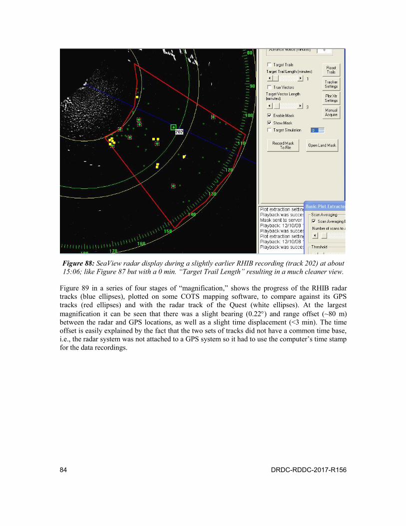
84 DRDC-RDDC-2017-R156
Figure 88: SeaView radar display during a slightly earlier RHIB recording (track 202) at about 15:06; like Figure 87 but with a 0 min. “Target Trail Length” resulting in a much cleaner view.
Figure 89 in a series of four stages of “magnification,” shows the progress of the RHIB radar tracks (blue ellipses), plotted on some COTS mapping software, to compare against its GPS tracks (red ellipses) and with the radar track of the Quest (white ellipses). At the largest magnification it can be seen that there was a slight bearing (0.22) and range offset (~80 m) between the radar and GPS locations, as well as a slight time displacement (<3 min). The time offset is easily explained by the fact that the two sets of tracks did not have a common time base, i.e., the radar system was not attached to a GPS system so it had to use the computer’s time stamp for the data recordings.

DRDC-RDDC-2017-R156 85
Figure 89: Radar (blue) and GPS (red) tracks for the RHIB; the white ellipses represent the radar track for the Quest. There was a slight
bearing (0.22) and range offset (~80 m) between the radar and GPS locations, as well as a slight displacement in time (<3min.). The series of plots are gradually zoomed in to show the most detail in the lower right.
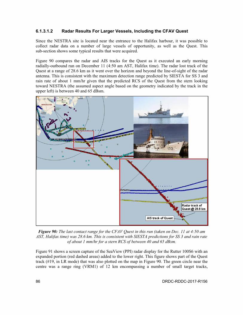
86 DRDC-RDDC-2017-R156
6.1.3.1.2 Radar Results For Larger Vessels, Including the CFAV Quest
Since the NESTRA site is located near the entrance to the Halifax harbour, it was possible to collect radar data on a number of large vessels of opportunity, as well as the Quest. This sub-section shows some typical results that were acquired.
Figure 90 compares the radar and AIS tracks for the Quest as it executed an early morning radially-outbound run on December 11 (4:50 am AST, Halifax time). The radar lost track of the Quest at a range of 28.6 km as it went over the horizon and beyond the line-of-sight of the radar antenna. This is consistent with the maximum detection range predicted by SIESTA for SS 3 and rain rate of about 1 mm/hr given that the predicted RCS of the Quest from the stern looking toward NESTRA (the assumed aspect angle based on the geometry indicated by the track in the upper left) is between 40 and 65 dBsm.
Figure 90: The last contact range for the CFAV Quest in this run (taken on Dec. 11 at 4:50 am
AST, Halifax time) was 28.6 km. This is consistent with SIESTA predictions for SS 3 and rain rate of about 1 mm/hr for a stern RCS of between 40 and 65 dBsm.
Figure 91 shows a screen capture of the SeaView (PPI) radar display for the Rutter 100S6 with an expanded portion (red dashed areas) added to the lower right. This figure shows part of the Quest track (#19, in LR mode) that was also plotted on the map in Figure 90. The green circle near the centre was a range ring (VRM1) of 12 km encompassing a number of small target tracks,

DRDC-RDDC-2017-R156 87
presumably from lobster or fishing boats. Note that the date shown in the upper right corner of the figure was ahead by 1 day; it should have displayed 09/12/2008. This was due to an incorrect initial setting on the computer that was maintained during the trials for consistency.
Figure 91: Rutter 100S6 SeaView PPI display with an expanded portion from showing the CFAV
Quest radar track (#19) which also plotted in Figure 90.
Figure 92 shows the same outbound track (with a timeline) as well as some earlier manoeuvres performed by the Quest at 3:42:32 Atlantic Time, on 11-Dec. It is clear from the plot, that the radar was easily able to maintain a track on the Quest as it executed a complex 360° turn with a radius of less than 120 m at a range of about 12.5 km.
Figure 93 compares the AIS and radar tracks (LR mode) of the Quest as it executed a simple 360° manoeuvre at a range of 14.5 km from NESTRA. The purple and white markers for the radar tracks are respectively before and after slight corrections were made to the radars range and bearing estimates to make the tracks align with the AIS reports.
Figure 94 shows a radar track (LR mode) of the Quest for the early morning (just after sunrise) of 11-Dec. as it made a radially inbound run from 50 km out at sea. The radar began tracking the ship at around 25 km which was reasonable considering that the bow aspect angle presents a much smaller RCS of 35 to 45 dBsm; it is also easier for the tracker to maintain an outbound track than it is to initiate an inbound track. The Sea State at this time was between 2 and 3 with a rain rate of about 1 mm/hr.
As mentioned earlier, a number of vessels of opportunity were tracked during the NESTRA trials. Figure 95 shows the radar track (LR mode) acquired for the Algoscotia on the morning of 11-Dec when the Sea-State was 2 to 3 and the rain rate was roughly 1 mm/hr. The radar started tracking the vessel at a range of 28.2 km, which is consistent with the maximum detection range of a vessel

88 DRDC-RDDC-2017-R156
of this size which (based on photo dimensions) has deck housing up to 29 m above the sea surface. Also, the ship’s longitudinal axis was at an oblique angle to the radar beam which usually results in a lower RCS than at broadside or end-on. Tracking the Algoscotia—as with the Quest—was limited by the LOS afforded by the low altitude of the NESTRA radar site. Figure 96 shows a screen capture of the radar display while the Algoscotia was being tracked in LR mode.
Figure 92: Radar (light & dark blue ellipses) and AIS (black dots) tracks for the CFAV Quest on the morning of 11-Dec. 2008. The inset in the lower left is an expanded view of vessel manoeuvre
showing how well the radar tracked the ship during a complex manoeuvre with a turn radius of less than 120 m.

DRDC-RDDC-2017-R156 89
Figure 93: Tight turn of radius 150 m executed by the CFAV Quest, captured by both the AIS
(light blue triangles) and the radar (purple and white). The purple and white markers are respectively before and after slight corrections were made to the radar range and bearing
estimates. The centre of the circle is at 14.5 km from NESTRA.
Figure 94: More radar (white ellipses) and AIS (red) tracks for the Quest from the morning of
11-Dec. The radar began tracking the ship at around 25 km when the Sea-State was between 2 and 3 with a rain rate of about 1 mm/hr.

90 DRDC-RDDC-2017-R156
Figure 95: AIS (green) and Radar (red) tracks for the Algoscotia on the morning of 11-Dec.
The Sea State was 2 to 3 and rain rate was roughly 1 mm/hr. The maximum detection range of 28.2 km is consistent with a vessel of this size and aspect with respect to the radar-to-target
geometry. The photos of the Algoscotia on the right are courtesy of Tim Hammond.
Figure 96: PPI display from SeaView for the inbound Algoscotia plotted in Figure 95.

DRDC-RDDC-2017-R156 91
Figure 97 and Figure 98 provide plots of the radar tracks (LR mode) acquired from two large container ships, the OOCL San Francisco and the Zim Pusan, observed on the morning of 10-Dec. The OOCL ship was tracked to a maximum range of 42.5 km and the Zim Pusan was tracked to a maximum range of 35 km during SS 1-2 conditions with no precipitation. These ranges are consistent with SIESTA predictions for the coverage, with given the target-to-radar geometry.
Figure 97: Radar+AIS tracks of two large container ships, the inbound OOCL San Francisco
(two photos, upper right) and outbound Zim Pusan (two photos, lower right). The first was detected at 9:49 am Dec. 10 at 33.6 km; the latter at 10:02 am the same day at a range of 35 km.
The conditions were SS 1 to 2 with no precipitation. (Photos courtesy of Tim Hammond).

92 DRDC-RDDC-2017-R156
Figure 98: Radar+AIS tracks of the outbound OOCL San Francisco on Thursday morning,
11-Dec. 2008 with SS 2-3 and a rain rate of 1–2 mm/hr. The maximum detection range of the ship is consistent with its size (stern approx. 26 m ASL) and the SIESTA predictions in Figure 37.
6.1.3.1.3 Radar Results for Aircraft
While the primary objective of the NESTRA trials was to evaluate the sensors against marine targets, there were at least three or four air targets of opportunity observed. Based on their apparent course two of these (shown in Figure 99 and Figure 100) were probably destined for Shearwater AFB and were probably Sea Kings helicopters that were travelling at rates of speed between 50 and 110 knots.
Figure 101 provides a series of image captures of the radar display showing the progress of an aircraft of unknown type detected by the radar. The series of plots is used to show the aircraft location because the alpha-beta tracker for the Rutter 100S6 had a problem locking on due to echo fades and land clutter interference. The sequence of plots is ordered by the number shown in the upper right corner of each display.

DRDC-RDDC-2017-R156 93
Figure 99: Track (green) of an aircraft bisecting the red automatic target acquisition zone, the
apparent heading to Shearwater AFB at about 110 knots. Although the radar could easily detect the target, the tracker had difficulty maintaining the track. Each range ring is spaced by 3 Nm.
Figure 100: Track of an aircraft/helicopter (MR mode) heading toward Shearwater AFB. The
target course is outlined with a white polygon to highlight the radar tracks, and where the radar lost track as the aircraft made a sharp manoeuvre around the CFAV Quest (yellow dot at the
bend). Each range ring is spaced 3nmi (5.6 km).

94 DRDC-RDDC-2017-R156
Figure 101: Series of radar plots showing the progress of an aircraft (highlighted in each image by a white circle centred on the aircraft echo) of unknown type. The series of plots is used to show the aircraft location because the tracker had a problem locking on due to fades
and land clutter interference. The sequence of plots is ordered by the number shown in the upper right corner of each display.
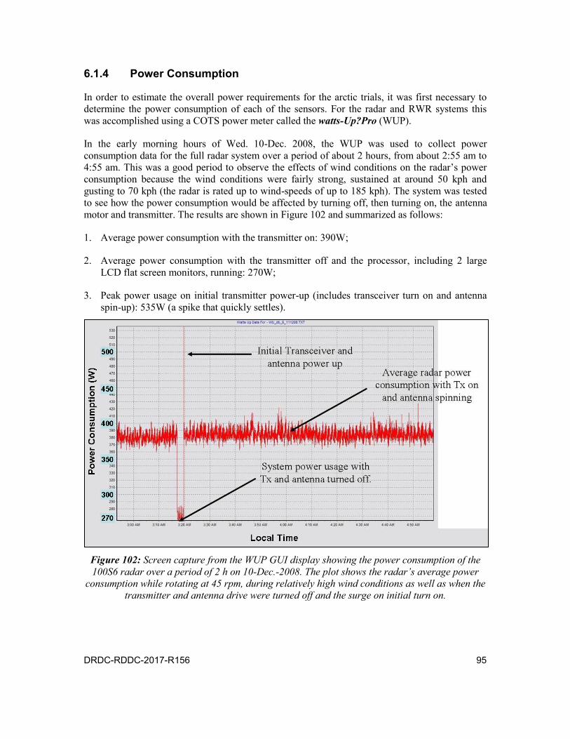
DRDC-RDDC-2017-R156 95
6.1.4 Power Consumption
In order to estimate the overall power requirements for the arctic trials, it was first necessary to determine the power consumption of each of the sensors. For the radar and RWR systems this was accomplished using a COTS power meter called the watts-Up?Pro (WUP).
In the early morning hours of Wed. 10-Dec. 2008, the WUP was used to collect power consumption data for the full radar system over a period of about 2 hours, from about 2:55 am to 4:55 am. This was a good period to observe the effects of wind conditions on the radar’s power consumption because the wind conditions were fairly strong, sustained at around 50 kph and gusting to 70 kph (the radar is rated up to wind-speeds of up to 185 kph). The system was tested to see how the power consumption would be affected by turning off, then turning on, the antenna motor and transmitter. The results are shown in Figure 102 and summarized as follows:
1. Average power consumption with the transmitter on: 390W;
2. Average power consumption with the transmitter off and the processor, including 2 large LCD flat screen monitors, running: 270W;
3. Peak power usage on initial transmitter power-up (includes transceiver turn on and antenna spin-up): 535W (a spike that quickly settles).
Figure 102: Screen capture from the WUP GUI display showing the power consumption of the 100S6 radar over a period of 2 h on 10-Dec.-2008. The plot shows the radar’s average power
consumption while rotating at 45 rpm, during relatively high wind conditions as well as when the transmitter and antenna drive were turned off and the surge on initial turn on.
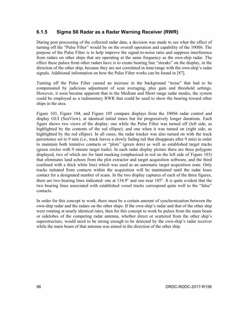
96 DRDC-RDDC-2017-R156
6.1.5 Sigma S6 Radar as a Radar Warning Receiver (RWR)
During post processing of the collected radar data, a decision was made to see what the effect of turning off the “Pulse Filter” would be on the overall operation and capability of the 100S6. The purpose of the Pulse Filter is to help improve the signal-to-noise ratio and suppress interference from radars on other ships that are operating at the same frequency as the own-ship radar. The effect these pulses from other radars have is to create bearing line “streaks” on the display, in the direction of the other ship, because they are not correlated in time/range with the own-ship’s radar signals. Additional information on how the Pulse Filter works can be found in [87].
Turning off the Pulse Filter caused an increase in the background “noise” that had to be compensated by judicious adjustment of scan averaging, plus gain and threshold settings. However, it soon became apparent that in the Medium and Short range radar modes, the system could be employed as a rudimentary RWR that could be used to show the bearing toward other ships in the area.
Figure 103, Figure 104, and Figure 105 compare displays from the 100S6 radar control and display GUI (SeaView), at identical initial times but for progressively longer durations. Each figure shows two views of the display: one while the Pulse Filter was turned off (left side, as highlighted by the contents of the red ellipse); and one when it was turned on (right side, as highlighted by the red ellipse). In all cases, the radar tracker was also turned on with the track persistence set to 9 min (i.e., track leaves a slowly fading tail that disappears after 9 min) in order to maintain both tentative contacts or “plots” (green dots) as well as established target tracks (green circles with 9 minute target trails). In each radar display picture there are three polygons displayed, two of which are for land masking (emphasized in red on the left side of Figure 103) that eliminates land echoes from the plot extractor and target acquisition software, and the third (outlined with a thick white line) which was used as an automatic target acquisition zone. Only tracks initiated from contacts within the acquisition will be maintained until the radar loses contact for a designated number of scans. In the two display captures of each of the three figures, there are two bearing lines indicated: one at 134.9 and one near 185. It is quite evident that the two bearing lines associated with established vessel tracks correspond quite well to the “false” contacts.
In order for this concept to work, there must be a certain amount of synchronization between the own-ship radar and the radars on the other ships. If the own-ship’s radar and that of the other ship were rotating at nearly identical rates, then for this concept to work be pulses from the main beam or sidelobes of the competing radar antenna, whether direct or scattered from the other ship’s superstructure, would need to be strong enough to be detected by the own-ship’s radar receiver while the main beam of that antenna was aimed in the direction of the other ship.

DRDC-RDDC-2017-R156 97
Figure 103: Screen captures showing the 100S6 radar control and display GUI when the
“Pulse Filter” option was turned off (left), and then on (right) over the same period (9 Dec. 2008, 14:28:02). The red oval in the upper left of each disp lay shows the
location and status of the control “button.” Most of the “false” plots on the left align with two green bearing lines (135 and 184) that also coincide with the bearings of ships
presumably with similar X-band navigation radars.
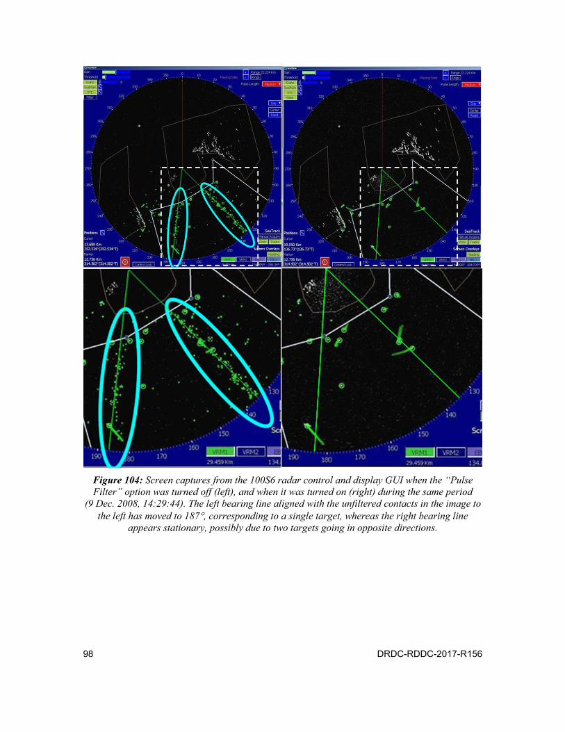
98 DRDC-RDDC-2017-R156
Figure 104: Screen captures from the 100S6 radar control and display GUI when the “Pulse Filter” option was turned off (left), and when it was turned on (right) during the same period
(9 Dec. 2008, 14:29:44). The left bearing line aligned with the unfiltered contacts in the image to the left has moved to 187, corresponding to a single target, whereas the right bearing line
appears stationary, possibly due to two targets going in opposite directions.
DRDC-RDDC-2017-R156 99
Figure 105: Screen captures from the 100S6 radar control and display GUI when the “Pulse Filter” option was turned off (left), and when it was turned on (right) during the same period
(9 Dec. 2008, 14:32:37). As the target ship on the right changes bearing (e.g.,185 to 190), the “false” plots accumulate over the sector swept out by the bearing line.
There are only certain conditions under which the radar will be capable of providing a bearing line to other radar emitters and associated platforms:
1. The transmitted carrier frequencies of the “target” radar emitters must be within the bandwidth of the local radar receiver (note: most non-coherent X-band navigation radars operate at a frequency of 9410 MHz within a bandwidth of 20 to 30 MHz);
2. There must be a direct line of sight between the local radar and the target emitters; and
3. The target emitters must be transmitting toward the local radar either through their main beams, sufficiently strong sidelobes, or from pulses reflected from the ship’s superstructure while the local radar’s main beam is pointed at them; this means that for the first two

100 DRDC-RDDC-2017-R156
conditions the pointing angles of the local and target systems must be appropriately synchronized to the extent that the following relationship is true:
Pointing-Direction Local Radar ± 0.5 BW=Pointing-Direction Target Radar ± Nth sidelobe-direction (4)
In Equation (4), BW is the azimuthal beamwidth of the radar and the value of N will depend on the strength of the sidelobe and the distance between the local and the target radar systems.
If the local radar is only to act as a tripwire at a shipping chokepoint, then the synchronization requirement in the last constraint will be less stringent:
Pointing-DirectionLocal Radar ±(0.5 BW+)=Pointing-DirectionTarget Radar ± Nth sidelobe-direction (5)
The value of will depend on the heading of the target emitter’s platform/vessel, the heights of above sea level of the local and target radar antennas and the distance between the two antennas. Since it is a one way propagation path between the target emitter and the local radar, the maximum observable LOS range of the target emitter is only limited by the horizon and is given by Equation (1). For example, if the local radar was sited on top of Cape Liddon at 300 m ASL, the ship’s radar was at a height of 20 m ASL, and the ship was on an East to West course 45 km south of Cape Liddon, then the maximum LOS range would be about 90 km, resulting in a value of about 60°. Therefore, in this case, even though the two radar systems could have antennas that were out of synchronization by more than 120° the local radar would detect the target radar at some point along the course shown by the green arrow in Figure 106.

DRDC-RDDC-2017-R156 101
Figure 106: Relative geometry for estimating the synchronization constraints between the local
and target radar antennas to use the local radar as an RWR.

102 DRDC-RDDC-2017-R156
7 Observations and Conclusions
The following general observations can be made from the results of the NESTRA 2008 trials:
1. Based on the observed performance, under normal conditions the radar should be able to detect and track small vessels (e.g., small tugboats, and fishing vessels) to a distance of about 12 km;
2. The radar was able to accurately track the Quest through complex manoeuvres at distances of up to 15 km; complex manoeuvres were not performed beyond this range except for course changes performed at ~50 km which were well beyond the LOS distance to the horizon;
3. The radar was able to track the Quest to just beyond the LOS distance to the horizon which is, under Standard Earth conditions, about 22 km from the radar site;
4. Larger container vessels could be tracked by the radar to distances over 40 km, which was almost twice the LOS distance to the horizon. This is due to the fact that the superstructure of such ships are roughly the same height above the water as the radar sensor;
5. The radar was able to track a stationary marine buoy out to a distance of 19 km, showing the utility of scan averaging for slow moving or stationary targets;
6. The radar was able to detect and accurately track the RHIB at a distance of up to 11 km although it was difficult to know definitively whether the corner reflector on the RHIB was trained toward the radar site all of the time and how much it contributed to this tracking capability;
7. Only one RHIB tracking run was possible during the trial because of the adverse weather conditions, therefore it was not possible to do an accurate calibration trial with the corner reflector;
8. Unfortunately the radar was not in continuous operation so during some shut-down periods some large vessels of opportunity, as shown by the recorded AIS tracks, were not tracked.
9. In general, coverage area, and the target detection capability of the Rutter radar system was predicted reasonably well using the SIESTA prediction software.
It may be useful to have multiple processors to process the data in parallel in order to optimize tracking of different types of targets and at different ranges for the following reasons:
1. For a quickly moving target (e.g., air target or fast boat) scan averaging will have little benefit and in fact may prove a hindrance. One of the reasons for using scan averaging is to reduce the effects of clutter echoes from the sea surface due to wave action. Since wave action is non-stationary, scan averaging tends to enhance the detection of a stationary or slow moving target, by “averaging” away the wave echoes. While it won’t remove them completely, it will improve the effective signal to clutter ratio. On the other hand for fast moving targets that are small compared to the a typical range-azimuth cell, scan averaging will have a detrimental

DRDC-RDDC-2017-R156 103
effect on target tracking by reducing the effective signal strength by a target. It will result in smearing the target or in the worst case for a scan average value of N it will create N-1 ghost images each with 1/N of the original strength.
2. For fast moving targets, as long as pulse integration is not sufficiently degraded, the fastest scan rate available should be chosen since it will provide the best update rate for the tracker. In this case it was set to a scan rate of 45 rpm.
3. Depending on the size and range of the target to be detected and tracked, it may be more effective to have different threshold settings for different range intervals. For example, despite the use of STC to improve the dynamic range of the radar display and reduce near-in sea clutter, the background still tends to be higher at close ranges thus requiring the detection threshold to be set high enough to remove the clutter, while not removing the target. However, for targets at greater ranges where the background clutter is reduced, the signal may also be relatively weak and would be removed if the detection threshold is set too high. On the other hand, a threshold that is set to optimize the detection and tracking of a weak target at longer ranges may result in unacceptable numbers of false plots and tracks at close range that can saturate the tracker capacity.
4. For the Arctic, it may be useful to determine some pre-arranged settings for automatic acquisition zones, sensitivity-time-control (STC) settings and constant-false-alarm-rate (CFAR) settings depending on the weather conditions at the time. For example, if wind conditions (speed and direction) and sea state are known, then different acquisition zones might be automatically selected to optimize the radars effectiveness.
When the “Pulse Filter” is turned off, it is possible to use the navigation radar as a rudimentary radar warning receiver (RWR) system for identifying the bearing of other X-band navigation radars operating in same frequency. The system will also perform best when operating in either short range mode or medium range mode because the radar will be sampling at a higher rate than in long range mode, i.e., 3000 Hz for short range and 1800 Hz for medium range versus only 785 Hz in the long range mode. Although there would have been no safety concerns related to transmitting over a full 360 of azimuth, during the trial’s data collection, the radar transmission was blanked over a sector of about 180, facing West of the system, to avoid irradiating the NESTRA building and personnel directly behind the radar. The remaining un-blanked arc of 180 still allowed for monitoring the Quest, as well as vessel traffic in the NESTRA and Halifax Harbour areas. If one wanted to operate the system in a stealth mode, i.e., no transmission, but passively receiving signals from other radars, the blanking sector could be increased to a full 360.
Whenever possible, the radar should be operated with a GPS signal feed in order to provide an accurate time base and site location. At a minimum the radar’s position should be manually input to the system, to avoid tracking errors.
In future it would be useful to have an orientation sensor (e.g., compass) attached to the radar’s base or to have at least two stationary targets or landmarks of known position to serve as calibration for orienting the radar display. Normally the orientation of the display is based on input from the ship’s other navigation sensors and the actual orientation of the radar’s base consisting of the transceiver and drive box. However, during the 2008 NESTRA trials, there were

104 DRDC-RDDC-2017-R156
no other external sensors, GPS or otherwise, attached to the radar, and because of the way the radar was mounted on top of the truck, it may have been vulnerable to slight changes in orientation due to the buffeting of the wind; the effects of the wind on the truck were easily felt, and this was one of the reasons for the metal stabilizers placed beneath the trucks cargo section (one on the left side and 2 on the right), to reduce rocking from the wind.
Scan averaging is mostly only useful for targets affected by sea clutter and that have a speed or size such that at least part of their radar echo remains in the same range-azimuth cell during multiple scans.
Some aircraft were observed during a couple of the runs, showing the potential for this system to track low flying aircraft. One was detected over the land to the Northeast, whereas two others were observed heading into the Shearwater AFB, approaching from the harbour entrance.
It is beyond the intended scope of this report to go into any detail, especially since there was a re-scoping of the NW Project’s objectives in 2009, but the AWS data that were collected and analysed from this set of trials were critical to understanding some of the technical and logistical challenges that the NW Science Team would later encounter in other Arctic trials in 2012 and during the final demonstration in 2015. More information on the outcomes of these trials and a summary of the project’s final accomplishments can be found in [88][89][90].
DRDC-RDDC-2017-R156 105
References
[1] Brookes, D., Forand, J.L., Northern Watch: Options Analysis to Select a Southern Test Site for Above Water Sensors, Technical Memorandum, DRDC Ottawa TM 2013-141, Defence R&D Canada – Ottawa, December 2013, 104 pages.
[2] Skolnik, M.I. (1980), Introduction to Radar Systems, 2nd ed., McGraw-Hill Inc., p. 44.
[3] Brookes, D., Campbell, B., Helleur, C., Jassemi-Zargani, R., Gingel, M. (2007), A Case for Service Oriented Architecture in Support of Arctic C4ISR, Fusion 2007 Conference, 8 pages.
[4] Brookes, D., Campbell, B., Helleur, C., Jassemi-Zargani, R., Gingel, M. (2007), An Examination of Service Oriented Architecture in Support of Arctic C4ISR, In Proceedings of the First Northern Watch Conference and Exposition on Arctic C4ISR.
[5] Brookes, D. (editor/organizer/co-author), The First Northern Watch Conference and Exposition on Arctic C4ISR, Dalhousie University, Halifax, Canada, 22–23 October 2007, Conference Proceedings on CD-ROM, CP-2008-003.
[6] Forand, J.L., Brookes, D., Lee, J., Heard, G., McCoy, N., MacLeod, M., Dao, R., Kollenberg, K. (2008), Surveillance of Canada’s High Arctic, Oceans ‘08 Conference, Quebec City.
[7] Forand, J.L (presenter/co-author)., Brookes, D., Lee, J., Heard, G., McCoy, N., MacLeod, M., Dao, R., Kollenberg K. (2008), Surveillance of Canada’s High Arctic, Oceans ‘08 Conference, Quebec City, Presentation http://www.arcticnet.ulaval.ca/pdf/talks2007/Forand.pdf (Access date: 25-Oct-2011).
[8] Avis, P. (Captain (N)), Surveillance and Canadian Maritime Domestic Security, Canadian Military Journal, Spring 2003, 6 pages, (Date Modified: 2008-07-14) http://www.journal.forces.gc.ca/vo4/no1/policy-police-eng.asp (Access date: 10-Aug-2014).
[9] Szeker, R.G. (2009), RF SIESTA software user manual: Version V09-4, Contractor Report, DRDC Ottawa CR 2009-138, Defence R&D Canada – Ottawa.
[10] Technologies OBZERV Inc (2008), CANDISS CDR Document W7701-7-1678; Northern Watch EO Imaging Systems, Technical Specifications.
[11] Turcotte, C.S. (Spectral and Geospatial Exploitation) (2009), Optics at Defence R&D Canada – Valcartier: Photonics Toolkit, PowerPoint Presentation, 27 slides http://www.repol.copl.ulaval.ca/toolkit/ressources/DRDC_Valcartier_(Turcotte).pdf (Access date: 13-Aug-2015).
[12] Heard, G.J., Kennedy, T., McInnis, J. (2006), Rapid Deployable Systems (RDS) for Underwater Surveillance: Final Report (MacDonald Detwiler), DRDC Contractor Report, CR 2006-223, Defence R&D Canada.

106 DRDC-RDDC-2017-R156
[13] Ebbeson, G.R., Heard, G., Desharnais, F., Matthews, M.R., Dosso, S. (2007), Array Element Localization of a Rapidly Deployable System of Sensors: AEL Final Report for the RDS TDP, Technical Memorandum, DRDC Atlantic TM 2007-009, Defence R&D Canada – Atlantic.
[14] Ebbeson, G.R., Heard, G.J., Desharnais, F., Lucas, C.E., Matthews, M-N.R. (2007), Hardware and Software Progress in Deployable Systems, In Proceedings of the 36th Technical Cooperation Program Maritime Panel TP-9, The Technical Cooperation Program.
[15] Heard, G.J. (2008), Rapidly Deployable Systems Array Technology. DRDC Atlantic Fact Sheet NetALS0108, http://www.omnitechelectronics.ca/products/under-watersystems/custom-sensor-arrays.html (Access date: 13-Jul-2015).
[16] http://www.omnitechelectronics.ca/products/digital-arrays.html (Access date: 13-Jul-2015).
[17] Heard, G.J., Pelavas, N., Lucas, C.E., Peraza, I., Clark, D., Cameron, C., Shepeta, V. (2011), Development Of Low-Cost Underwater Acoustic Array Systems For The Northern Watch Technology Demonstration Project, In Canadian Acoustics Proceedings of the Acoustics Week in Canada 2011, Canadian Acoustical Association, Vol. 39 No. 3 (2011), pp. 200–201 http://jcaa.caa-aca.ca/index.php/jcaa/article/viewFile/2480/2229 (Access date: 13-Jul-2015).
[18] Heard, G.J., Pelavas, N., Lucas, C.E., Peraza, I., Schattschneider, G., Clark, D., Cameron, C., Shepeta, V. (2011), Developing An Underwater Acoustic Array System For The Northern Watch Technology Demonstration Project, In Proceedings of the 40th Technical Cooperation Program Maritime Panel TP-9, The Technical Cooperation Program, 2011.
[19] Canadian Space Agency (2013), The RADARSAT Constellation Mission, Brochure http://www.asc-csa.gc.ca/pdf/RADARSAT_constellation_eng.pdf (Access date: 24-Jan-2014).
[20] McHugh-Warren, S.L, Simms, É.L., Eye in the sky—Radar Images in the Prosecution of Illegal Oil Discharges: Opportunities and a Case Study, Journal of Ocean Technology 2012, Oil on Water, Vol. 7, No. 4, 2012, 14 pages, http://core.ac.uk/download/pdf/11701025.pdf (Access date: 14-Aug-2015).
[21] Transport Canada, Spill Prevention: National Aerial Surveillance Program, (Date Modified: 24-Feb-2012) http://www.tc.gc.ca/eng/marinesafety/oep-ers-nasp-2195.htm (Access date: 1-Nov-2013).
[22] Brookes, D., Campbell, B., Helleur, C., Jassemi-Zargani, R., Gingell, M., A Case for Service-Oriented Architecture in Support of Arctic C4ISR, Proceedings of 10th International Conference on Information Fusion, 9–12 July 2007, 8 pages.
DRDC-RDDC-2017-R156 107
[23] Canadian Space Agency, Maritime Monitoring and Messaging Micro-Satellite (M3MSat), (Date Modified: 24 April 2015), http://www.asc-csa.gc.ca/eng/satellites/m3msat/ (Access date: 12-Oct-2015).
[24] Wilson, L.S., The DEW LINE Sites in Canada, Alaska & Greenland, http://www.lswilson.ca/dewline.htm (Access date: 10-Dec-2013).
[25] Kerr, D.E. (1951), Propagation of Short Radio Waves (Volume 13 of the MIT Radiation Laboratory Series), New York: McGraw Hill Book Co., Chapter 7.
[26] Nohara, T., “Homeland Security Low-cost AccipiterTM Radar Surveillance Along Waterways,” December 2004, http://www.sicomsystems.com (Access date: 30-Aug-2006).
[27] IHS Global Limited (IHS.com), C4ISR & Mission Systems: Air: AN/FPS-117 air defence radar (Date Posted: 01-Sep-2005) https://janes.ihs.com/CustomPages/Janes/DisplayPage.aspx?DocType=Reference&ItemId=+++1541264 (Access date: 17-Nov-2014).
[28] IHS Global Limited (HIS.com), C4ISR & Mission Systems: Land: AN/FPS-124(V) surveillance radar (Date Posted: 22-Jun-2005) https://janes.ihs.com/CustomPages/Janes/DisplayPage.aspx?DocType=Reference&ItemId=+++1532596&Pubabbrev=JC4IL (Access date: 17-Mar-2015).
[29] Riseborough, E.S. (2008), Detection of low observables with a low cost navigation radar, Technical Report, DRDC Ottawa TR 2008-267, Defence R&D Canada – Ottawa.
[30] Scarlett, P. (2001), “Search and Rescue Tracker, Radar Data Processing and Performance Analysis,” Raytheon TP#13803, prepared for Transport Canada by Raytheon Canada Limited.
[31] Bhattacharya, T.K., Nohara, T.J., Premji, A., Weber, P., Currie, B. (McMaster University), Ryan, J. (Sigma Engineering Ltd.) (1998), Cross-Polarized Radar Processing, SICOM Systems Ltd, TP-13263e http://www.tc.gc.ca/innovation/tdc/publication/13200/13263e.pdf (Access date: 25 Sept. 2009).
[32] Surveillance Systems Press Releases: New SharpEye™ Coastal Surveillance/VTS Radar from Kelvin Hughes, (Date Posted: 20 Sep 2007) http://www.kelvinhughes.com/surveillance/news/press-releases/202-new-sharpeye-coastal-surveillancevts-radar-from-kelvin-hughes (Access date: 6-June-2009).
[33] Hughes, K. (2008), SharpEye: Technical Specifications, Brochure http://www.shipserv.com/ShipServ/pages/attachments/82347/SharpEye_issue4.pdf (Access date: 6-June-2009).
[34] https://www.kelvinhughes.com/news/204-type-approval-for-latest-sharpeye (Access date: 11-Oct-2015).
[35] Briggs, J.N. (2004), Target Detection by Marine Radar, Stylus Publishing, LLC, pp. 379–385.

108 DRDC-RDDC-2017-R156
[36] Williams, P.D.L., Cramp, H.D., Curtis, K. (1978), Experimental study of the radar cross section of maritime targets, IEE Electronic Circuits and Systems, Vol. 2. No 4, pp. 121–136.
[37] Joint Task Force North (JTFN) J2, 2008 Shipping Summary.
[38] IMO Pilot 2006 (The periodical information on technical and operational IMO legislation) Results from IMO sessions MSC80 and MEP 53included, 6th edition, Germanischer Lloyd 2006 http://www.tes.bam.de/aktuelles/news_docs_2006/IMO_Pilot_2006.pdf (Access date: 30-Nov-2007).
[39] MCA Marine and Coastal Agency, Marine Guidance Note MGN 349 (M+F): Carriage and Use of Radar Reflectors on Small Vessels-Notice to all Owners, Operators, Masters and Skippers of small vessels under 150 tons including Pleasure craft. http://www.sea-me.co.uk/pdf/Guidance.pdf (Access date: 29-Jan-2009).
[40] Luke, S. (QINETIQ/D&TS/SEA/CR0704527/2.0) (2007), Performance investigation of marine radar reflectors on the market, QinetiQ Ltd, Cody Technology Park, Farnborough, Hampshire http://www.ussailing.org/wp-content/uploads/daroot/Offshore/SAS Studies/2007 Radar Reflector Test.pdf (Access date: 19-Feb-2011).
[41] Brookes, D., Campbell, B., Helleur, C., Jassemi-Zargani, R., Gingell, M., A Case for Service-Oriented Architecture in Support of Arctic C4ISR, In Proceedings of 10th International Conference on Information Fusion, 9–12 July 2007.
[42] Sea-Hawk, Sea-Hawk Radar-SHN4000 Radar, Brochure, 14-May-2011 http://sea-hawk.com/products/shn-4000/Sea-Hawk_SHN_4000_Oil_Spill_Rev_C1_May_2011.pdf (Access date: 19-Oct-2012).
[43] Sea-Hawk, Sea-Hawk Radar-SHN3300 Radar, Brochure, 14 May 2011, 3 pages http://sea-hawk.com/products/shn-3300/Sea-Hawk_SHN_3300_Rev_C1_May_2011.pdf (Access date: 19-Oct-2012).
[44] Hughes, K., Delivering Detection Solutions: Mantadigital- Radar Detection Systems for Navigation, Oil Spill Detection and Security, Brochure (Manta Digital Oil Spill Detection System) (Date Posted: 13-Mar-2011), http://kelvinhughes.com/marine/applications/Oil_spill_detection_and_security_oil-spotting.pdf (Access date: 19-Oct-2012).
[45] Safer, A. (2011), Marine Technology Reporter (MTR) magazine (17 February 2011), The View from St. John’s: Ice and Oil-Spill Detection, MTR#1, pp. 14–17 http://andrew.safer.com/Ice_Oil_Spill_Detection.pdf or Specialized_Radar_for_Ice_and_Oil-Spill_Detection.pdf (Access date: 19-Oct-2012).
[46] Rutter Inc. (2012), Port Technology International magazine (www.porttechnology.org), Detecting oil on water using microwave radar http://www.rutter.ca/wp-content/uploads/2012/01/Detecting_oil_on_water_using_microwave_radar.pdf (Access date: 17 Jan 2013).

DRDC-RDDC-2017-R156 109
[47] Rutter Inc (2012, Specialized Radar for Ice and Oil-Spill Detection http://www.rutter.ca/wp-content/uploads/2012/01/Specialized_Radar_for_Ice_and_Oil-Spill_Detection1.pdf (Access date: 17-Jan-2013).
[48] Rutter Inc. (2012), Detecting Oil Using Combined Radar and Infrared Sensors by Aptomar, http://www.rutter.ca/wp-content/uploads/2012/01/Detecting_Oil_Using_Combined_Radar_and_Infrared_Sensors_by_Aptomar.pdf (Access date: 17-Jan-2013).
[49] Rutter Inc. (2012), Detecting Offshore Oil Spills with Rutter Technologies Sigma S6 Radar Technology http://www.rutter.ca/wp-content/uploads/2012/01/Detecting_Offshore_Oil_Spills_with_Rutter_Technologies_Sigma_S6_Radar_Technology.pdf (Access date: 17-Jan-2013).
[50] Rutter Inc. (2012), Innovation in Rutter’s Oil Spill Management System http://www.rutter.ca/wp-content/uploads/2012/01/Innovation_in_Rutters_Oil_Spill_Management_System.pdf (Access date: 17-Jan-2013).
[51] Rutter Inc., sigma S6 Oil Spill Detection (OSD) System, White Paper, 8-Nov-2013, 7 pages http://www.rutter.ca/uploads/default/files/d861a18f697b9c677d852330adacaac5.pdf (Access date: 15-Aug-2015).
[52] Rutter Inc. http://www.rutter.ca/sigma_s6_oil_spill_response/ (Access date: 15-Aug-2015).
[53] Batelle Memorial Institute (Batelle) (2014), “Report: Capabilities and Uses of Sensor-Equipped Ocean Vehicles for Subsea and Surface Detection and Tracking of Oil Spills, OGP-IPIECA Oil Spill Response Joint Industry Project, Surveillance, Modelling & Visualization Work Package 1: In Water Surveillance” http://oilspillresponseproject.org/sites/default/files/uploads/report_ogp-ipieca_osr_jip_wp1____in_water_surveillance_13nov2014_v1.0.pdf (Access date: 15-Aug-2015).
[54] http://www.porttechnology.org/technical_papers/detecting_oil_on_water_using_microwave_radar/#download_article (Access date: 15-Aug-2015).
[55] Rutter Inc. (2013), sigma S6 Oil Spill Detection (OSD) System, White Paper http://www.rutter.ca/uploads/default/files/d861a18f697b9c677d852330adacaac5.pdf (Access date: 15-Aug-2015).
[56] Brookes, D. (2013), Northern Watch: Air Surveillance With a Rutter 100S6 Radar—System-Trials, Analysis, and Results, Technical Memorandum, DRDC Ottawa TM 2013-152, Defence R&D Canada – Ottawa.
[57] Specification for the DHC-6 Twin Otter, Copyright 2002, XdH Aviation Services Inc., http://www.xdh.ca/DHC_Aircraft/DHC-6/dhc-6.html (Access date: 20-Jun-2009).
110 DRDC-RDDC-2017-R156
[58] Ridenour, L.N. (ed.): Radar System Engineering, MIT Radiation Laboratory Series, Vol. 1, McGraw-Hill Book Company, New York, 1947, page 76.
[59] B-26 Marauder Historical Society, Copyright 2005-2013, Mote Marketing Inc. http://www.b-26mhs.org (Access date: 12-Jun-2013).
[60] Skolnik, M.I. (2008), Radar Handbook, 3rd Edition, New York: McGraw-Hill, p. 14.13.
[61] Naval Research Advisory Committee: Lighter-Than-Air Systems for Future Naval Missions, Brief given to Flag Officers and Senior Executive Service, 4-Oct.-2005 Pentagon Auditorium, from http://www.onr.navy.mil/nrac/docs/2005_brief_lighter_than_air.pdf (Access date: Dec-2007).
[62] Brookes, D., Scott, D.F., Rudkin, P. (2013), Arctic Surveillance: Civilian Commercial Aerial Surveillance of the Arctic, Technical Report, DRDC Ottawa TR 2013-142, Defence R&D Canada – Ottawa.
[63] Forand, J.L., Larochelle, V., Brookes, D., Lee, J. (2009), “Northern Watch Halifax 2008 Test: Q-317A Cruise Plan,” Technical Note, DRDC Valcartier TN 2008-363, Defence R&D Canada – Valcartier.
[64] Legault, S., Boivin, D. (2006), “Summary of RCS measurements for Q289A, September 13–15 2005,” Technical Note, DRDC Ottawa TN 2006-277, Defence R&D Canada – Ottawa.
[65] Ruck, G.T. (1970), Radar Cross Section Handbook, New York: Plenum Press, Vol. 2, p. 591.
[66] Skolnik, M.I. (2008), Radar Handbook, 3rd Ed., New York: McGraw-Hill, p. 14.11.
[67] Robertson, S.D. (1947), Targets for Microwave Radar Navigation, Bell System Technical Journal, Vol. 26, pp 852–869.
[68] http://syros-observer.aegean.gr/ais/showallphotos.aspx?mmsi=211311970&language=_GR&language=_GR#top_photo (Access date: 6-Jan-2009).
[69] Photographs and ship’s specifications for CCGS Sir William Alexandre http://www.ccg-gcc.gc.ca/eng/Fleet/Vessels?id=968&info=6 and www.vesseltracker.com/en/ShipPhotos/252092-Sir-William-Alexandr-8320482.html (Access date: 1-Jun-2009).
[70] Photographs of the Skandi Bergen http://www.vesseltracker.com/en/ShipPhotos/123798-Skandi-Bergen-9374260.html (Access date: 1-Jun-2009).
[71] Photographs and ship’s specifications for the Rega http://www.digital-seas.com/vessel_search/vessel_details/on/c6sp2_rega_q51039.html?tx_fleetmonportal_pi1%5Bposition%5D=8#photos (Access date: 1-Jun-2009).

DRDC-RDDC-2017-R156 111
[72] Photographs and ship’s specifications for the Undine http://www.marinetraffic.com/ais/showallphotos.aspx?mmsi=265884000#top_photo (Access date: 11-Jun-2009).
[73] Atlantic Towing Limited (brochure): Atlantic Bear Specifications (bear_2009.pdf) http://www.atlantictowing.com (Access date: 11-Jun-2009).
[74] Photographs and ship’s specifications for the OOCL San Francisco http://www.vesseltracker.com/en/ShipPhotos/24079-Oocl-San-Francisco-9199268.html (Access date: 11-Jun-2009).
[75] Photographs and ship’s specifications for the Sirius Highway http://www.vesseltracker.com/en/ShipPhotos/88128-Sirius-Highway-8406042.html (Access date: 11-Jun-2009).
[76] Photographs and ship’s specifications for the Zim Pusan http://www.marinetraffic.com/AIS/shipdetails.aspx?MMSI=235007670 (Access date: 1-Jun-2009).
[77] Photographs and ship’s specifications for the British Courtesy http://www.vesseltracker.com (Access date: 11-Jun-2009).
[78] Photographs and ship’s specifications for the Maria Desgagnes http://www.marinetraffic.com/ais/shipdetails.aspx?mmsi=316285000 (Access date: 1-Jun-2009).
[79] Photographs and ship’s specifications for the Atlantic Superior http://www.marinetraffic.com/ais/shipdetails.aspx?mmsi=311000171 (Access date: 11-Jun-2009).
[80] Photographs and ship’s specifications for the Nirint Force http://www.vesseltracker.com (Access date: 11-Jun-2009).
[81] Photographs and ship’s specifications for the Svitzer Bedford (photo by M. MacKay) http://tugfaxblogspotcom.blogspot.ca/2010_07_01_archive.html (Access date: 7-Oct-2010).
[82] Capnkens Blog: Tanker Traffic at Halifax, (Photograph of the Kometik) http://capnkensblog.blogspot.ca/2010/07/tanker-traffic-at-halifax.html (Access date: 7-Oct-2010).
[83] Photograph and ship’s specifications for the Atlantic Oak (photo by M. MacKay) http://tugfaxblogspotcom.blogspot.ca/2010_09_01_archive.html (Access date: 7-Oct-2010).
[84] Sigma S6 / SeaScan Technical Manual, Rutter Technologies Inc., SIG-UM-04-001 Rev.2.0, Initial Issue Date: 20 March 1998, Revision Issue Date: 24 February 2005.
112 DRDC-RDDC-2017-R156
[85] Atlantic Coast 2009 – List of Lights, Buoys and Fog Signals: Nova Scotia Southeast Coast, Fisheries and Oceans Canada – Canadian Coast Guard, (Date Modified: 1-Sep-2013) http://www.notmar.gc.ca/eng/services/list/2009-atlantic-coast/a327e2009.pdf (Access date: 20-Sep-2013).
[86] National Data Buoy Center – Station 44258, National Oceanic and Atmospheric Administration (NOAA) http://www.ndbc.noaa.gov/station_page.php?station=44258 (Access date: 15-Jan-2009).
[87] Rutter Technologies Inc., Sigma S6 /SeaView Operators Manual-E-SP-01180 Rev. 2.0; Appendix 1: Theory of Operation, p. 61.
[88] Flatt, G. (MDA Systems Ltd), System Design Description for Northern Watch Technology Demonstration Project: CDRL TR 003, Contractor Report, DRDC-RDDC-2016-C305, Defence Research and Development Canada, October 2014, 101 pages.
[89] McArthur, B., Pelavas, N., Heard, G., Cross, R., Brookes, D., Lee, J., Roy, S., Forand, L., Northern Watch sensor performance trial—Summary of collected data and preliminary findings; Scientific Report, DRDC-RDDC-2015-R252, Defence Research and Development Canada, December 2015, 238 pages.
[90] Heard, G.J., McArthur, B., Inglis, G., Overview of the technical results of the Northern Watch Project, Scientific Report, DRDC-RDDC-2016-R115, Defence Research and Development Canada, June 2016, 106 pages.
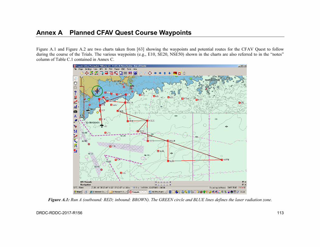
DRDC-RDDC-2017-R156 113
Planned CFAV Quest Course Waypoints Annex A
Figure A.1 and Figure A.2 are two charts taken from [63] showing the waypoints and potential routes for the CFAV Quest to follow during the course of the Trials. The various waypoints (e.g., E10, SE20, NSE50) shown in the charts are also referred to in the “notes” column of Table C.1 contained in Annex C.
Figure A.1: Run A (outbound: RED; inbound: BROWN). The GREEN circle and BLUE lines defines the laser radiation zone.

114 DRDC-RDDC-2017-R156
Figure A.2: Run B (outbound: RED; inbound: BROWN). The GREEN circle and BLUE lines defines the laser radiation zone.

DRDC-RDDC-2017-R156 115
Rutter 100S6 Radar System Description and Annex BSpecifications
The radar system used for the NESTRA 2008 Trials was a non-coherent marine navigation radar purchased from Rutter Technologies Inc. of St. John’s NL. The major components of the system are comprised of Rutter’s proprietary “back-end” processing system and a Sperry-Marine BridgeMaster-E “front end” antenna and transceiver. The core of the back-end processing unit is the Sigma S6 card which digitizes the analog output from the transceiver front-end allowing for further signal processing, such as scan averaging to reduce the effects of sea and weather clutter, to enhance persistent, slower moving targets. The card also facilitates storage of raw radar data for later playback and post-processing as if in real-time (RT).
Although known generically as the Rutter 100S6 Radar system, it can come in any of several possible combinations of software and hardware depending on the user’s requirements. The configuration that was purchased for the Northern Watch project consisted of the following:
Hardware: Server Processor:
2.8 GHz Pentium 4 Processor with 2 GB RAM. Sigma S6 video signal processor card;
Sperry-Marine BridgeMaster-E 25 kW (peak) X-band (941030 MHz) radar transceiver with antenna drive and gearbox: item# RUT-01034-AA-0091; Meets Industry Canada Type Approval certification requirements
(spec. RSS138) as evidenced by IC Certificate No. 2907381104 issued to LITTON MARINE SYSTEMS B.V. on 20 April 1999.
2.4 m (8 foot) slotted waveguide antenna.
Software: Operating System:
Windows XP-Pro, Service Pack 2. Rutter Software:
Sigma S6 server (12 bit and 8 bit options): SeaScan12.exe or SeaScan8.exe; SeaScanRCU.exe: configuration utility for Sigma S6; SeaView: GUI for controlling the radar, signal processing options and providing
radar PPI display with plots and tracks; SeaTrack version 2.07.50: tracking software.
ICAN:
Horizon Electronic Chart System (ECS): shore based management software for Vessel Traffic Services (VTS) centres that can be interfaced with AIS and ARPA radar systems to track marine vessel traffic.

116 DRDC-RDDC-2017-R156
Some of the key features of the Rutter system are as follows:
Through its client-server architecture, it allows the operator to network radar data and send it to multiple PCs at different locations where the radar image display may be viewed and manipulated according to each user’s preference. This facilitates a scalable interconnected radar network. The system architecture is shown in Figure B.1.
The system offers optional tracking software, including SeaTrack 15, SeaTrack 50 (our version), SeaTrack 300, and SeaTrack 1000. The latter is capable of tracking up to 1024 targets and includes a dual-mode plot extractor that enables it to detect and track small, slow- and high-speed targets at the same time.
The system offers optional recording capabilities for recording raw data at the full dynamic range and resolution. The recordings can be played back to show real incidents as if they were occurring in RT thus supporting post-trials analysis.
For maximum flexibility, the system also came with a switch to choose between two optional antenna rotation speeds, either 28 rpm or 45 rpm scanning rates. And a 2.4 m (8 foot) antenna was acquired with the system to provide the highest directional gain available from the company. Tracking software (SeaTrack50) was also provided with the system which was capable of handling 50 target tracks at a time.
The heart of the radar processor is based on Rutter’s Sigma S6 Radar Signal input (Rsi) video processor card which is plugged into a standard desktop PC and performs the high speed digitization (up to 80M samples/sec, as required) and signal processing of the analog video output from the transceiver. This allows the radar data to be stored in a very raw format so that a very realistic copy of the original analog signal can be re-generated later for post processing as if it were the original transceiver video signal.
As stated, an important consideration when purchasing this radar system was its stated capability to be networked over a TC/IP connection. To quote from their Operator’s Manual:
“Through its client-server architecture, the Sigma S6 System allows the operator to network radar data and send it to multiple PCs at different locations where the radar image display may be viewed and manipulated according to each user’s preferences.” The Sigma S6 architecture is shown in Figure B.1.
“The server PC runs the sigma S6 Server software which communicates directly with the Rsi card. The server PC retrieves the radar data and forwards it to the sigma S6 SeaView software. SeaView displays the processed digital radar images and is the main operator interface.
The SeaView software can run on the server PC or on a Client PC that is connected to the server PC through a local area network (LAN) or over the internet. In this way multiple networked Client PCs can display radar images from multiple radar scanners.
The sigma S6 System also includes plot extraction and target tracker software (SeaTrack) modules. These modules can be used with the SeaView software for target tracking. The sigma S6 System plot extractor and SeaTrack software run in the PC background and display their output in the SeaView application window.

DRDC-RDDC-2017-R156 117
The sigma S6 plot extractor takes digitized radar data directly from the sigma S6 Server software and determines the parts of the image that fit the defined values to upgrade it to a plot (precursor to a track). It sends the upgraded data as plot images to the sigma S6 SeaTrack software. SeaTrack assesses the plot images to determine if the plot should be upgraded to a track. The SeaTrack software then extracts the upgraded tracking information and sends it to the SeaView software for display.”
Radar Hardware (Composite
or Separate Signals)
CVD Card Hardware
RSi Card Hardware
S6 Server Software Plot
Extractor Software
SeaTrack Software
Composite
SeaView Software
Scan Image
Scan Image
Separated Signals
Radar Server PC Client PC(s)
Figure B.1: Rutter 100S6 radar network architecture.
The specifications for the radar are provided in Table B.1 and Table B.2.
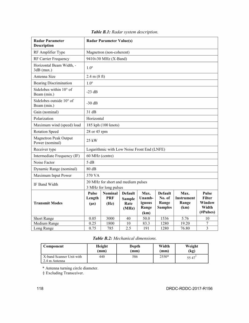
118 DRDC-RDDC-2017-R156
Table B.1: Radar system description.
Radar Parameter Description
Radar Parameter Value(s)
RF Amplifier Type Magnetron (non-coherent) RF Carrier Frequency 9410±30 MHz (X-Band) Horizontal Beam Width, -3dB (max.) 1.0
Antenna Size 2.4 m (8 ft) Bearing Discrimination 1.0 Sidelobes within 10° of Beam (min.) -23 dB
Sidelobes outside 10° of Beam (min.) -30 dB
Gain (nominal) 31 dB Polarization Horizontal Maximum wind (speed) load 185 kph (100 knots) Rotation Speed 28 or 45 rpm Magnetron Peak Output Power (nominal) 25 kW
Receiver type Logarithmic with Low Noise Front End (LNFE) Intermediate Frequency (IF) 60 MHz (centre) Noise Factor 5 dB Dynamic Range (nominal) 80 dB Maximum Input Power 370 VA
IF Band Width 20 MHz for short and medium pulses 3 MHz for long pulses
Transmit Modes
Pulse Length
(µs)
Nominal PRF (Hz)
Default Sample
Rate (MHz)
Max. Unamb-iguous Range (km)
Default No. of Range
Samples
Max. Instrument
Range (km)
Pulse Filter
Window Width
(#Pulses) Short Range 0.05 3000 40 50.0 1536 5.76 10 Medium Range 0.25 1800 10 83.3 1280 19.20 7 Long Range 0.75 785 2.5 191 1280 76.80 3
Table B.2: Mechanical dimensions.
Component Height (mm)
Depth (mm)
Width (mm)
Weight (kg)
X-band Scanner Unit with 2.4 m Antenna
440 586 2550* 55 47‡
* Antenna turning circle diameter. ‡ Excluding Transceiver.
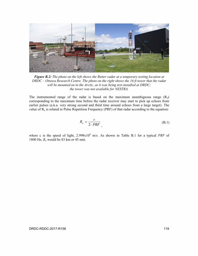
DRDC-RDDC-2017-R156 119
Figure B.2: The photo on the left shows the Rutter radar at a temporary testing location at
DRDC – Ottawa Research Centre. The photo on the right shows the 16 ft tower that the radar will be mounted on in the Arctic, as it was being test-installed at DRDC;
the tower was not available for NESTRA.
The instrumented range of the radar is based on the maximum unambiguous range (Ru) corresponding to the maximum time before the radar receiver may start to pick up echoes from earlier pulses (a.k.a. very strong second and third time around echoes from a large target). The value of Ru is related to Pulse Repetition Frequency (PRF) of that radar according to the equation:
PRFcRu
2 , (B.1)
where c is the speed of light, 2.998x10⁸ m/s. As shown in Table B.1 for a typical PRF of 1800 Hz, Ru would be 83 km or 45 nmi.
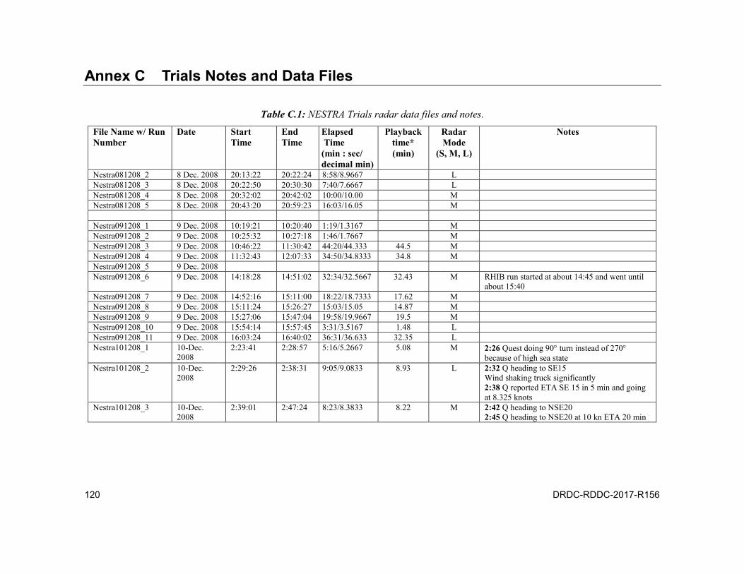
120 DRDC-RDDC-2017-R156
Trials Notes and Data Files Annex C
Table C.1: NESTRA Trials radar data files and notes.
File Name w/ Run Number
Date Start Time
End Time
Elapsed Time (min : sec/ decimal min)
Playback time* (min)
Radar Mode
(S, M, L)
Notes
Nestra081208_2 8 Dec. 2008 20:13:22 20:22:24 8:58/8.9667 L Nestra081208_3 8 Dec. 2008 20:22:50 20:30:30 7:40/7.6667 L Nestra081208_4 8 Dec. 2008 20:32:02 20:42:02 10:00/10.00 M Nestra081208_5 8 Dec. 2008 20:43:20 20:59:23 16:03/16.05 M Nestra091208_1 9 Dec. 2008 10:19:21 10:20:40 1:19/1.3167 M Nestra091208_2 9 Dec. 2008 10:25:32 10:27:18 1:46/1.7667 M Nestra091208_3 9 Dec. 2008 10:46:22 11:30:42 44:20/44.333 44.5 M Nestra091208_4 9 Dec. 2008 11:32:43 12:07:33 34:50/34.8333 34.8 M Nestra091208_5 9 Dec. 2008 Nestra091208_6 9 Dec. 2008 14:18:28 14:51:02 32:34/32.5667 32.43 M RHIB run started at about 14:45 and went until
about 15:40 Nestra091208_7 9 Dec. 2008 14:52:16 15:11:00 18:22/18.7333 17.62 M Nestra091208_8 9 Dec. 2008 15:11:24 15:26:27 15:03/15.05 14.87 M Nestra091208_9 9 Dec. 2008 15:27:06 15:47:04 19:58/19.9667 19.5 M Nestra091208_10 9 Dec. 2008 15:54:14 15:57:45 3:31/3.5167 1.48 L Nestra091208_11 9 Dec. 2008 16:03:24 16:40:02 36:31/36.633 32.35 L Nestra101208_1 10-Dec.
2008 2:23:41 2:28:57 5:16/5.2667 5.08 M 2:26 Quest doing 90 turn instead of 270
because of high sea state Nestra101208_2 10-Dec.
2008 2:29:26 2:38:31 9:05/9.0833 8.93 L 2:32 Q heading to SE15
Wind shaking truck significantly 2:38 Q reported ETA SE 15 in 5 min and going at 8.325 knots
Nestra101208_3 10-Dec. 2008
2:39:01 2:47:24 8:23/8.3833 8.22 M 2:42 Q heading to NSE20 2:45 Q heading to NSE20 at 10 kn ETA 20 min
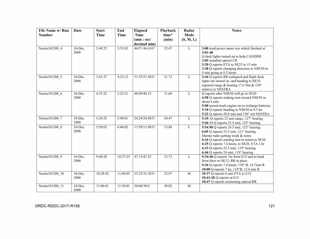
DRDC-RDDC-2017-R156 121
File Name w/ Run Number
Date Start Time
End Time
Elapsed Time (min : sec/ decimal min)
Playback time* (min)
Radar Mode
(S, M, L)
Notes
Nestra101208_4 10-Dec. 2008
2:48:25 3:35:02 4637:/46.6167 32.47 L 3:00 tried power meter test which finished at 3:01:40 Q deck lights turned on to help CANDISS 3:05 installed optical CR 3:20 Q reports ETA to SE25 in 15 min 3:38 Q reports changing direction to NSE30 in 4 min going at 8.5 knots
Nestra101208_5 10-Dec. 2008
3:41:37 4:33:12 51:35/51.5833 31.73 L 3:44 Q reports RR realigned and flight deck lights are turned on, and heading to SE35, reported range & bearing 17.6 Nm & 130 relative to NESTRA
Nestra101208_6 10-Dec. 2008
4:35:22 5:23:31 48:09/48.15 31.68 L Q reports after NSE50 will go to SE20 4:58 Q reports making turn toward NSE50 in about 4 min 5:00 turned truck engine on to recharge batteries 5:10 Q reports heading to NSE50 at 8.5 kn 5:22 Q reports 20.8 nmi and 130 wrt NESTRA
Nestra101208_7 10-Dec. 2008
5:24:32 5:49:01 24:29/24.4833 24.47 L 5:35: Q reports 22 nmi range, 127 bearing 5:46:34 Q reports 23.5 nmi, 125 bearing
Nestra101208_8 10-Dec. 2008
5:50:03 6:04:02 13:59/13.9833 13.88 L 5:54:50 Q reports 24.5 nmi, 123 bearing 6:05 Q reports 25.5 nmi, 121 bearing Marine radio getting weak & noisy 6:16 Q reports starting turn to return to SE20 6:25 Q reports 7.4 knots, to SE20, ETA 2 hr 6:33 Q reports 22.5 nmi, 119 bearing 6:46 Q reports 24 nmi, 119 bearing
Nestra101208_9 10-Dec. 2008
9:40:20 10:27:35 47:15/47.25 32.73 L 9:34:46 Q reports 1hr from E15 and to head from there to SE12; RR in place 9:36 Q reports 7.4 knots, 118 B, 14.7nmi R 10:00 Q reports 7 kn, 118B, 12.6 nmi R
Nestra101208_10 10-Dec. 2008
10:28:42 11:04:05 35:23/35.3833 32.97 M 10:37 Q reports 6 min ETA to E15 10:41:20 Q reports at E15 10:47 Q reports reorienting optical RR
Nestra101208_11 10-Dec. 2008
11:06:01 11:36:01 30:00/30.0 30.02 M

122 DRDC-RDDC-2017-R156
File Name w/ Run Number
Date Start Time
End Time
Elapsed Time (min : sec/ decimal min)
Playback time* (min)
Radar Mode
(S, M, L)
Notes
Nestra101208_12 10-Dec. 2008
11:45:38 11:59:23 13:45/13.75 13.67 L 11:55:30 Q reports 6.45kn 132B
Nestra111208_1 11-Dec. 2008
2:15:01 3:24:03 69:02/69.0333 33.33 L 3:01 Q reports heading to NSE20 to do a 180 turn and head back to SE15, then to SE12 and will orient optical RR from Port to Starboard 3:08:30 Q reports 8.3 knots, turned to head to SE15 3:13 Q reports ETA 20 min 3:30 Q reports ETA SE12 in 1 min and proceeding at 8 knots 3:40:48 Q reports starting 540 turn 3:42 Had problem with SeaTrack S/W and had to reboot to see if it would fix the problem
Nestra111208_2 11-Dec. 2008
3:42:26 4:04:03 21:37/21.6167 21.62 L 3:48:11 Q reports heading to SE15 at 7.5kn with deck lights on and RR oriented to NESTRA 3:50 Q reports 7 min ETA to SE15 Sea Temp 6.5C and Air 4.3C and dropping from earlier reading of 5.5C.
Nestra111208_3 11-Dec. 2008
4:05:02 5:10:01 64:59/64.9833 32.83 L 4:16 Q reports reaching SE20 and proceeding to SE25 with ETA 20 min at 8.3 knots 4:27 Q at 8.4 kn with ETA 7 min to SE25 Decision made for Q to head to NSE50 to get back to SE25 by approx 7:00 to be ready for arrival of visitors from MWC. 4:43:53 last position of Q seen on radar at about 27 km range 5:05:50 Q reports 135T, 17.5 nmi
Nestra111208_4 11-Dec. 2008
5:17:02 6:07:02 50:00/50 32.77 L 5:18:45 Q reports 19.5 nmi, 135T 5:37 AlgoScotia detected at 25.6 km by Jim Lee. Q reports 135T, 21.7 nmi 5 :47 Q reports 135T, and 23 nmi 5 :49 Q reports ETA 20 min to SE50 6 :02 Q reports 25 nmi, 135T
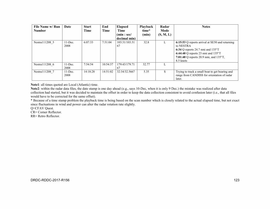
DRDC-RDDC-2017-R156 123
File Name w/ Run Number
Date Start Time
End Time
Elapsed Time (min : sec/ decimal min)
Playback time* (min)
Radar Mode
(S, M, L)
Notes
Nestra111208_5 11-Dec. 2008
6:07:33 7:51:04 103:31/103.5167
32.8 L 6:15:53 Q reports arrival at SE50 and returning to NESTRA 6:34 Q reports 24.7 nmi and 135T 6:44:40 Q reports 23 nmi and 135T 7:01:40 Q reports 20.9 nmi, and 135T, 8.5 knots
Nestra111208_6 11-Dec. 2008
7:54:54 10:54:37 179:43/179.7167
32.77 L
Nestra111208_7 11-Dec. 2008
14:18:28 14:51:02 32:34/32.5667 5.35 S Trying to track a small boat to get bearing and range from CANDISS for orientation of radar later.
Note1: all times quoted are Local (Atlantic) time. Note2: within the radar data files, the date stamp is one day ahead (e.g., says 10-Dec, when it is only 9 Dec.) the mistake was realized after data collection had started, but it was decided to maintain the offset in order to keep the data collection consistent to avoid confusion later (i.e., that all files would have to be corrected for the same offset). * Because of a time stamp problem the playback time is being based on the scan number which is closely related to the actual elapsed time, but not exact since fluctuations in wind and power can alter the radar rotation rate slightly. Q=CFAV Quest. CR= Corner Reflector. RR= Retro Reflector.

124 DRDC-RDDC-2017-R156
Typical Marine Vessel Traffic observed in the NWP 2003–2008 Annex D
Table D.1 provides a list of typical vessels that have been observed operating in arctic waters during the shipping season; the list is based on information covering the period of 2003 to 2008 that was obtained from DND’s “Global Position Warehouse,” a database of ships information and locations maintained by DND for the purposes of Maritime Domain Awareness (MDA). The table also includes information related to their size, the source of the size information (and pictures), and estimates of their RCS based on their gross tonnage (when available). Only some of the listed vessels have been seen in the vicinity of Resolute, or Barrow Strait during the period of 2005 to 2008, but the overall list does provide a good overview of the types of vessels that have operated in the Arctic Archipelago recently. Many of them have made repeated trips there or may be stationed there year round (e.g., tugboats). In general, for each category of vessel, they are listed in descending order of size based on gt, or on the ship’s length. It is likely true that most if not all of the sailboats listed will fall under 10dBsm due to their small size, and because in most instances their construction material is either predominantly wood or fibreglass. Their RCS will probably be determined mostly by the presence or absence of corner reflectors that are typically used as RCS enhancers for small vessels so that they can be seen by larger ships to avoid collisions in foggy conditions.
Table D.1: Listing of vessels observed to operate in arctic waters during the period 2003 to 2008 obtained from DND’s “Global Position Warehouse;” also included are their respective sizes, RCS estimates, the sources of the ship’s information, and any associated pictures.
Name Vessel Type
Length
(m)
Width (m)
Depth/ Draft (m)
Ship Size (gt)
RCS Estimate (dBsm)
Information Source Figure No.
Canadian Coast Guard Ship (CCGS)
Louis St. Laurent CCGS Icebreaker
119 24.4 9.8draft 6.4 fb
11345 34.0 to 48.3 http://www.ccg-gcc.gc.ca/eng/Fleet/Vessels?id=1111
Figure D.1
Henry Larsen CCGS Icebreaker
100 19.5 7.2 draft 3.8 fb
6166 31.8 to 45.1 http://www.ccg-gcc.gc.ca/e0003342 Figure D.2
Des Groseilliers CCGS Icebreaker
98.2 19.8 7.4draft 3.43 fb
6098 31.8 to 45.0 http://www.ccg-gcc.gc.ca/eng/Fleet/Vessels?id=1127
Figure D.3
Amundsen CCGS Icebreaker
98 19.5 7.2 draft 3.66 fb
5911 31.7 to 44.9 http://www.ccg-gcc.gc.ca/eng/Fleet/Vessels?id=1112&info=4
Figure D.4
Terry Fox CCGS Icebreaker
88 17.8 8.3draft 0.75fb
4234 30.5 to 43.2 http://www.ccg-gcc.gc.ca/eng/Fleet/Vessels?id=982&info=4
Figure D.5
Sir Wilfred Laurier CCGS Icebreaker
83 16.2 6 draft 3812 30.1 to 42.6 http://www.ccg-gcc.gc.ca/eng/Fleet/Vessel_pdf?id=1114&no_build=1
Figure D.6
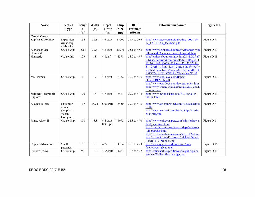
DRDC-RDDC-2017-R156 125
Name Vessel Type
Length
(m)
Width (m)
Depth/ Draft (m)
Ship Size (gt)
RCS Estimate (dBsm)
Information Source Figure No.
Cruise Vessels Kapitan Khlebnikov Expedition
cruise ship /icebreaker
134 26.8 8.6 draft 18000 35.7 to 50.6 http://www.zeco.com/upload/pdfac_2008-10-17_123113/KK_factsheet.pdf
Figure D.9
Alexander von Humboldt
Cruise Ship 152.5 20.6 4.5 draft 15271 35.1 to 49.8 http://www.shipparade.com/az/Alexander_von_Humboldt/Alexander_von_Humboldt.htm
Figure D.10
Hanseatic Cruise ship 123 18 4.8draft 8378 33.0 to 46.7 http://cruises.about.com/gi/o.htm?zi=1/XJ&zTi=1&sdn=cruises&cdn=travel&tm=38&gps=110_26_1163_996&f=00&su=p531.50.336.ip_&tt=29&bt=1&bts=1&st=24&zu=http%3A//www.hlkf.de/redwork/do.php%3Flayoutid%3D100%26node%3D39735%26language%3D2
Figure D.11
MS Bremen Cruise Ship 111 17 4.8 draft 6752 32.2 to 45.6 http://www.eurolloyd.com/Hapag-Lloyd/BREMEN.pdf http://www.eurolloyd.com/bremenreview.htm http://www.cruiseserver.net/travelpage/ships/hl_bremen.asp
Figure D.12
National Geographic Explorer
Cruise Ship 100 16 4.7 draft 6471 32.2 to 45.6 http://www.beyondships.com/NG-Explorer-Profile.html
Figure D.13
Akademik Ioffe
Passenger /research (geophys. /ocean biology)
117 18.24 6.09draft 6450 32.0 to 45.3 http://www.adventurefleet.com/fleet/akademik_ioffe http://www.newzeal.com/theme/Ships/Akademik/ioffe.htm
Figure D.7
Prince Albert II Cruise Ship 108 15.8 4.4 draft 8.9 depth
6072 31.8 to 45.0 http://www.cruisecompete.com/ships/prince_albert_ii_cruises.html http://silverseaships.com/cruiseships/silversea_albertcruise.html http://www.search2cruise.com/ship-1122.html http://z.about.com/d/cruises/1/0/k/H/4/Prince_Albert_II_2_Monaco.jpg
Figure D.14
Clipper Adventurer Small passenger
101 16.3 4.72 4364 30.6 to 43.3 http://www.quarkexpeditions.com/our-fleet/clipper-adventurer
Figure D.16
Lyubov Orlova Cruise Ship 90 16.2 4.65draft 4251 30.5 to 43.2 http://cruisenorthexpeditions.com/gallery/images/JeanWeller_Ship_ice_jpg.jpg
Figure D.16

126 DRDC-RDDC-2017-R156
Name Vessel Type
Length
(m)
Width (m)
Depth/ Draft (m)
Ship Size (gt)
RCS Estimate (dBsm)
Information Source Figure No.
(M/V) Explorer Cruise ship 75 14.2 4.5 draft 2398 28.4 to 40.2 http://www.adventurecanada.com/pdfs/antarctic2005.pdf http://www.shippingtimes.co.uk/images/explorer.jpg http://farm2.static.flickr.com/1082/941124452_e698de13f1.jpg
Figure D.8
Ocean Nova 73 11 3.7 draft 2118 27.9 to 39.6 http://www.travelwild.com/shipd/Ocean%20Nova/10004/ShipDetails.aspx
Figure D.15
Akademik Shokalskiy Cruise ship 71.6 12.6 4.5 draft 1764 27.3 to 38.7 http://www.quarkexpeditions.com/our-fleet/akademik-shokalskiy http://www.travelwild.com/shipd/Akademik%20Shokalskiy/10009/ShipDetails.aspx http://www.arctictopcruises.com/shokalskiy/ http://www.deepoceanexpeditions.com/tuamotu.pdf
Figure D.17
Amazon Express Yacht 67.3 10.6 4.82 1004 25.2 to 35.7 http://www.yachttrails.com/yachtspecs/see-yacht/amazon-express-397.html
Figure D.19
Icebreakers (not CCGS)
M/V Xue Long (a.k.a. Xuelong)
Research 167 22.6 9 draft 13.5 depth
10255 33.7 to 47.7 http://www.globalsecurity.org/military/systems/ship/icebreaker.htm http://www.chinare.cn/en/index.html?pid=stations&st=xuelong http://www.polarconservation.org/education/antarctic-ships/research-and-supply-vessels-arctic/china/M/V-xue-long
Figure D.18
Oden Icebreaker 108 29.4 12 depth to upper decks
9438 33.4 to 47.3 http://www.sjofartsverket.se/templates/SFVXPage____1077.aspx http://en.wikipedia.org/wiki/File:Swedish_icebreaker_Oden.jpg
Figure D.20
Arctic Kalvik/ Vladimir Ignatyuk (sister to Terry Fox)
Icebreaking tug
88 17.8 8.3draft 4234 30.5 to 43.2 http://www.journalofoceantechnology.com/getFile.asp?file=AHistoryOfIcebreakingShips.pdf&article=True&vol=3&issue=1
Cargo/Tanker Vessels

DRDC-RDDC-2017-R156 127
Name Vessel Type
Length
(m)
Width (m)
Depth/ Draft (m)
Ship Size (gt)
RCS Estimate (dBsm)
Information Source Figure No.
Aliacmon River Bulk Cargo /Fishing
181 30.5 15.3 depth 10.9 draft
22147 36.5 to 51.7 http://www.shipspotting.com/modules/myalbum/photo.php?lid=362225 http://www.clydesite.co.uk/articles/ship_management.asp http://www.iacs.org.uk/document/public/Ship_data/Suspension/PDF/Suspension_Dec_2005_pdf400.pdf
Figure D.21
Algosoo Cargo 219 23 12.6 21716 36.4 to 51.6 http://forms.cta-otc.gc.ca/sins-cvis/navire-ship_eng.cfm?ShipID=346839
Figure D.22
Anna Desgagnés
Cargo 173.5 23.1 13.7 moulded depth
17850 35.7 to 50.6 http://www.innovationmaritime.ca/An/droit/bulletin/Bulletin-pdf/33992%20Bulletin%20BioShip%20ang.pdf
Figure D.23
Brouwersgracht/ Scheldegracht
Cargo 172 24 16641 35.5 to 50.2 http://www.vesseltracker.com/en/Ships/Scheldegracht-9202510.html http://www.fleetmon.com/images/references/2780.jpg http://www.fleetmon.com/images/references/9182.jpg http://clydesights.com/2007_09_30_archive.html
Figure D.24
Key Ryu Bulk carrier 172 13706 34.8 to 49.2 http://www.shipsupply.ru/?xml=news&news_id=7566&news_cat=2
Figure D.25
Camilla Desgagnés Cargo 133 20.93 14.13 10085 33.6 to 47.6 http://www.wellandcanal.ca/shiparc/desgagnes/camilla/camilla.htm
Figure D.26
(M/T) Tellus Tanker 124 18 8.12 draft 7515 32.6 to 46.1 http://www.sirius-rederi.se/tellus.htm Figure D.27 Umiavut Bulk carrier 113 19.23 11.3 6037 31.8 to 45.0 http://www.wellandcanal.ca/salties/u/umiavut/
umiavut.htm Figure D.28
M/V Astron Small cargo 82 13.7 4.7 1746 27.2 to 38.6 http://forms.cta-otc.gc.ca/sins-cvis/navire-ship_eng.cfm?ShipID=341427
Figure D.30
Alex Gordon Off-shore supply
62.5 13.7 5.56 depth 4.33 draft
1190 25.8 to 36.6 http://www.ntcl.com/marine_operations/vessels.html
Figure D.29
Tugboats

128 DRDC-RDDC-2017-R156
Name Vessel Type
Length
(m)
Width (m)
Depth/ Draft (m)
Ship Size (gt)
RCS Estimate (dBsm)
Information Source Figure No.
Edgar Kotokak Tug 45.2 15.8 2.7 783 24.3 to 34.4 http://forms.cta-otc.gc.ca/sins-cvis/navire-ship_eng.cfm?ShipID=347537 http://www.ntcl.com/marine_operations/vessels.html http://www.ntcl.com/pdf/vessel-specs-edgar-henry.pdf
Figure D.31
Kitikmeot
Tug 48.8 12.2 2.8 669 23.7 to 33.6 http://forms.cta-otc.gc.ca/sins-cvis/navire-ship_eng.cfm?ShipID=330881
M/V Keewatin Tug 36.9 11.6 3.1 476 22.5 to 31.9 http://forms.cta-otc.gc.ca/sins-cvis/navire-ship_eng.cfm?ShipID=348028
Figure D.32
Atlantic Teak tug 29.8 9.1 4.3 draft) 310 20.9 to 29.6 http://www.shipspotting.com/modules/myalbum/photo-181224-Atlantic+Teak, http://www.atlantictowing.com/uploadedFiles/TEAK_2009_revised%20copy.pdf
Figure D.33
Eastern Tugger Tug 25.6 6.6 3.3 136 17.9 to 25.4 http://forms.cta-otc.gc.ca/sins-cvis/navire-ship_eng.cfm?ShipID=320753 http://www.shipspotting.com/modules/myalbum/photo-691923-EASTERN+TUGGER http://wwwapps.tc.gc.ca/saf-sec-sur/4/vrqs-srib/d.aspx?lang=e&vesselid=12769
Figure D.35
Kelly Ovayuak Tug 45.2 15.9 2.7 45.2 13.9 to 19.7 http://forms.cta-otc.gc.ca/sins-cvis/navire-ship_eng.cfm?ShipID=347535
Figure D.34
Other R/V Polar Stern (a.k.a. Polarstern)
Research Vessel
118 25 11.2 draft 17300 35.6 to 50.4 http://www.researchvessels.org/ship_info_display.asp?shipID=260 http://de.wikipedia.org/wiki/Polarstern_(Schiff) http://www.bsh.de/de/Meeresnutzung/Wissenschaft/Forschungsschiffe/Schiffseinsatzplaene/1085.jsp http://data.aad.gov.au/aadc/voyages/display_transport.cfm?transport_id=167
Arctic Endurance Arctic Shrimp Trawler
70 14.6 11.3 2793 29.0 to 41.0 http://www.st-as.no/arcticendurance.html Figure D.36

DRDC-RDDC-2017-R156 129
Name Vessel Type
Length
(m)
Width (m)
Depth/ Draft (m)
Ship Size (gt)
RCS Estimate (dBsm)
Information Source Figure No.
R/V Knorr Research Vessel
85 14 5 2518 28.6 to 40.5 http://www.whoi.edu/page.do?pid=8496 Figure D.37
R/V Geolog Dmitriy (Nalivkin)
Research Vessel
71.6 12.6 5.4 draft 1932 27.6 to 39.1 http://www.mage.ru/pic/nalb.jpg
Bin Hai 517 Oil exploration
60 15 1240 26.0 to 36.8 http://www.cosl.com.cn/full-range/binhai517.jsp
Figure D.39
M/V Paamiut Research vessel
53 722 24.0 to 34.0 http://archive.nafo.int/open/sc/2002/scr02-047.pdf
Aurora Magnetica Research Vessel
18.5 5.2 1.4 draft 40.5 13.5 to 19.1 http://www.researchvessels.org/ship_info_display.asp?shipID=989 http://www.auroramagnetica.com/architectural-characteristics/ http://www.auroramagnetica.com/labrador-07/labrador-kauk-harbour/
Figure D.41
R/V Strait Signet Seismic research/fishing vessel
32.1 8.6 4.3 322 21.1 to 29.8 http://forms.cta-otc.gc.ca/sins-cvis/navire-ship_eng.cfm?ShipID=328504
Figure D.40
Tiira Small trimaran
13.3 3.25 1.00 11 8.8 to 12.4 http://www.djurgardsvarvet.se/tugs/tiira/index.e.php?sold=true
R/V White Holly Research Vessel
40.5 9.1 2.7 draft N/K http://www.uscg.mil/history/webcutters/NPS_133_HAER_Report.pdf
Figure D.43
Southern Star Sailboat 23.7 5.6 2.4-4.2 N/K http://www.69nord.com/english/boat/index_eng.htm
Figure D.45
Baloum Gwen Sailboat 14.9 4.4 0.4-2.9 N/K http://www.arcticcalling.net/sailboat.html Figure D.42 Geraldine Converted
Maine Lobster boat
14 N/K http://www.M/Vgeraldine.com/the-boat/ Figure D.46
Arctic Wanderer Sailboat 11.9 N/K Figure D.44 Amodino Sailboat? N/K
gt= gross tonnage (volumetric measure); fb= freeboard; N/K=not known; M/V= motorized vessel; R/V= research vessel; CCGS=Canadian Coast Guard Ship.
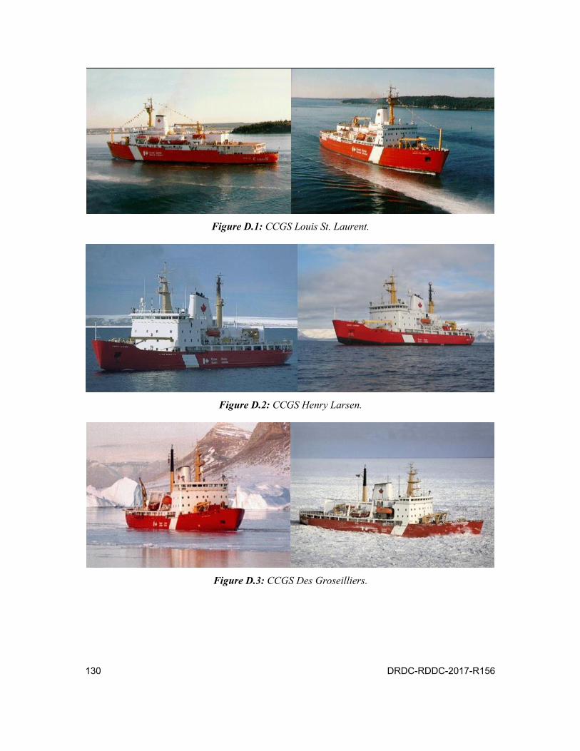
130 DRDC-RDDC-2017-R156
Figure D.1: CCGS Louis St. Laurent.
Figure D.2: CCGS Henry Larsen.
Figure D.3: CCGS Des Groseilliers.

DRDC-RDDC-2017-R156 131
Figure D.4: CCGS Amundsen.
Figure D.5: CCGS Terry Fox. Figure D.6: CCGS Sir Wilfred Laurier.
Figure D.7: Akademik Ioffe.
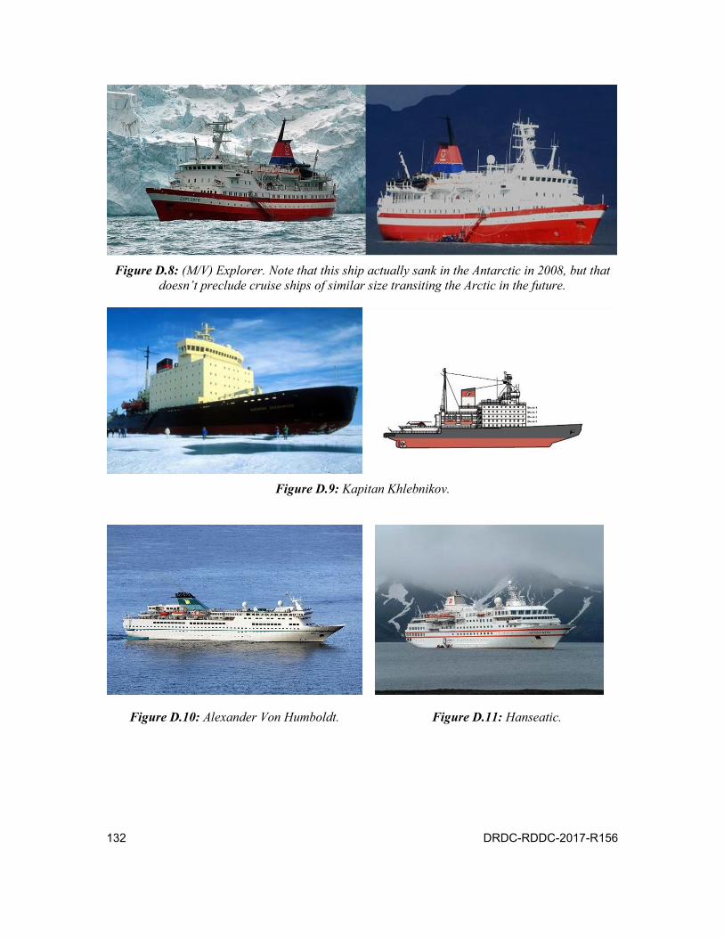
132 DRDC-RDDC-2017-R156
Figure D.8: (M/V) Explorer. Note that this ship actually sank in the Antarctic in 2008, but that
doesn’t preclude cruise ships of similar size transiting the Arctic in the future.
Figure D.9: Kapitan Khlebnikov.
Figure D.10: Alexander Von Humboldt. Figure D.11: Hanseatic.
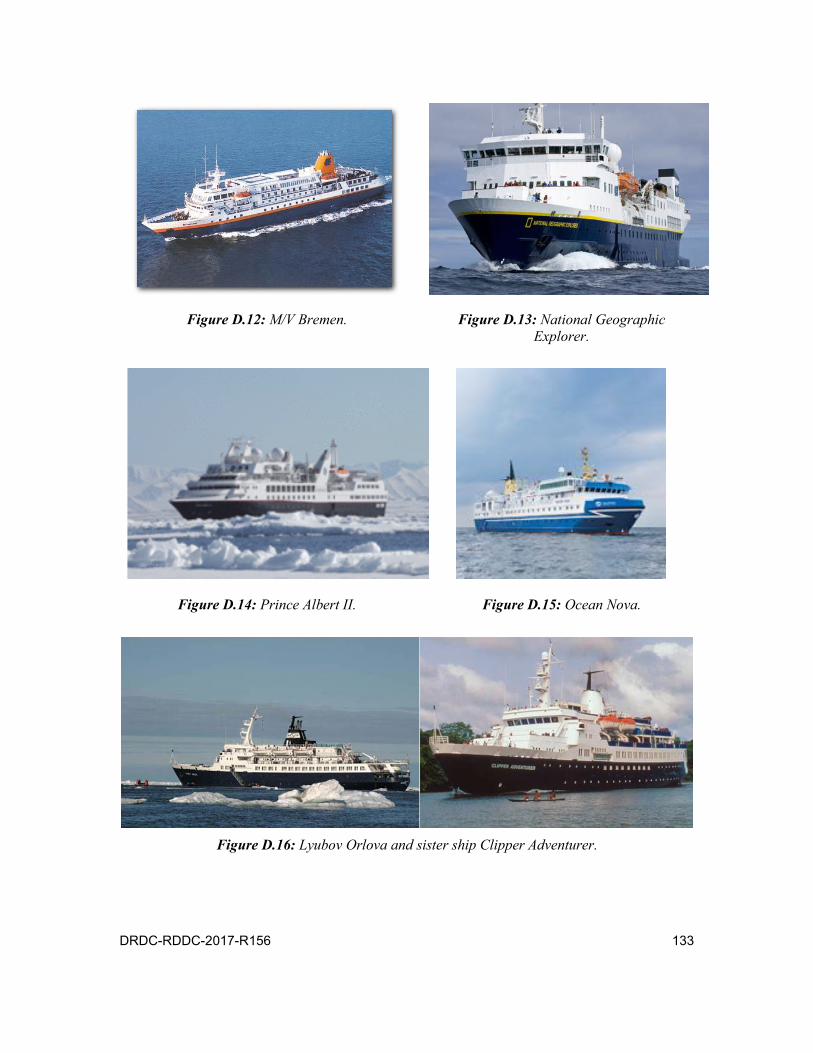
DRDC-RDDC-2017-R156 133
Figure D.12: M/V Bremen. Figure D.13: National Geographic Explorer.
Figure D.14: Prince Albert II. Figure D.15: Ocean Nova.
Figure D.16: Lyubov Orlova and sister ship Clipper Adventurer.

134 DRDC-RDDC-2017-R156
Figure D.17: Akademik Sholkaskiy. Figure D.18: R/V Xuelong.
Figure D.19: Amazon Express.
Figure D.20: Oden.
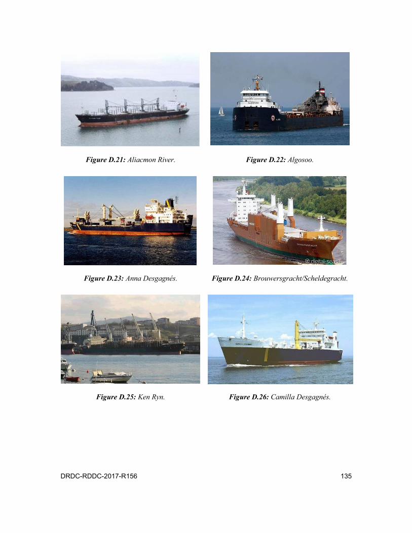
DRDC-RDDC-2017-R156 135
Figure D.21: Aliacmon River. Figure D.22: Algosoo.
Figure D.23: Anna Desgagnés. Figure D.24: Brouwersgracht/Scheldegracht.
Figure D.25: Ken Ryn. Figure D.26: Camilla Desgagnés.

136 DRDC-RDDC-2017-R156
Figure D.27: (M/T) Tellus. Figure D.28: Umiavut.
Figure D.29: M/V Astron. Figure D.30: Alex Gordon.
Figure D.31: Edgar Kotokak. Figure D.32: M/V Keewatin.

DRDC-RDDC-2017-R156 137
Figure D.33: Atlantic Teak. Figure D.34: Kelly Ovayuak.
Figure D.35: Eastern Tugger.
Figure D.36: Arctic Endurance.

138 DRDC-RDDC-2017-R156
Figure D.37: R/V Knorr. Figure D.38: R/V Geolog Dmitri.
Figure D.39: Bin Hai 517. Figure D.40: R/V Strait Signet.
Figure D.41: Aurora Magnetica. Figure D.42: Baloum Gwen.
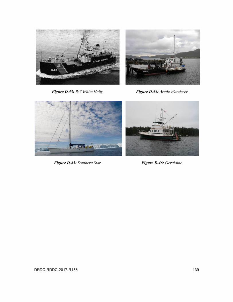
DRDC-RDDC-2017-R156 139
Figure D.43: R/V White Holly. Figure D.44: Arctic Wanderer.
Figure D.45: Southern Star. Figure D.46: Geraldine.
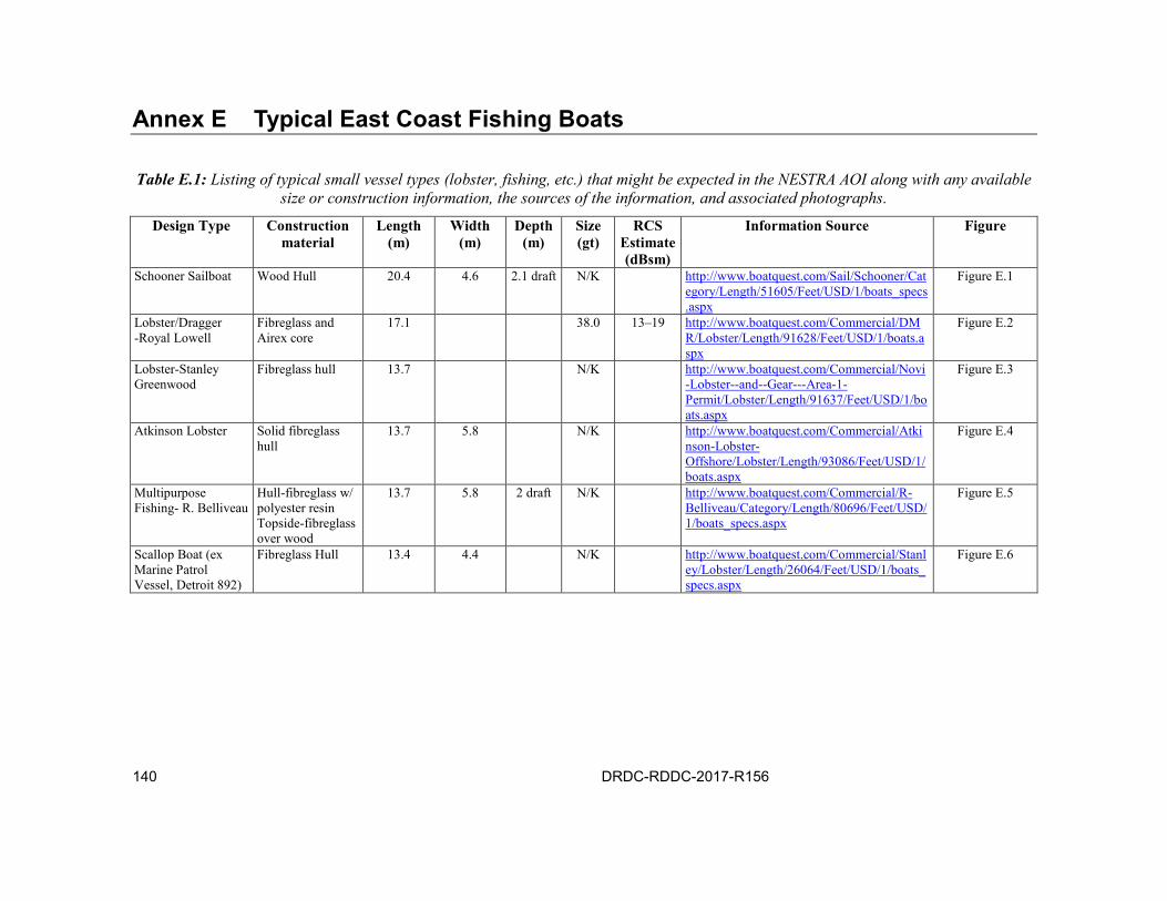
140 DRDC-RDDC-2017-R156
Typical East Coast Fishing Boats Annex E
Table E.1: Listing of typical small vessel types (lobster, fishing, etc.) that might be expected in the NESTRA AOI along with any available size or construction information, the sources of the information, and associated photographs.
Design Type Construction material
Length (m)
Width (m)
Depth (m)
Size (gt)
RCS Estimate (dBsm)
Information Source Figure
Schooner Sailboat Wood Hull 20.4 4.6 2.1 draft N/K http://www.boatquest.com/Sail/Schooner/Category/Length/51605/Feet/USD/1/boats_specs.aspx
Figure E.1
Lobster/Dragger -Royal Lowell
Fibreglass and Airex core
17.1 38.0 13–19 http://www.boatquest.com/Commercial/DMR/Lobster/Length/91628/Feet/USD/1/boats.aspx
Figure E.2
Lobster-Stanley Greenwood
Fibreglass hull 13.7 N/K http://www.boatquest.com/Commercial/Novi-Lobster--and--Gear---Area-1-Permit/Lobster/Length/91637/Feet/USD/1/boats.aspx
Figure E.3
Atkinson Lobster Solid fibreglass hull
13.7 5.8 N/K http://www.boatquest.com/Commercial/Atkinson-Lobster-Offshore/Lobster/Length/93086/Feet/USD/1/boats.aspx
Figure E.4
Multipurpose Fishing- R. Belliveau
Hull-fibreglass w/ polyester resin Topside-fibreglass over wood
13.7 5.8 2 draft N/K http://www.boatquest.com/Commercial/R-Belliveau/Category/Length/80696/Feet/USD/1/boats_specs.aspx
Figure E.5
Scallop Boat (ex Marine Patrol Vessel, Detroit 892)
Fibreglass Hull 13.4 4.4 N/K http://www.boatquest.com/Commercial/Stanley/Lobster/Length/26064/Feet/USD/1/boats_specs.aspx
Figure E.6
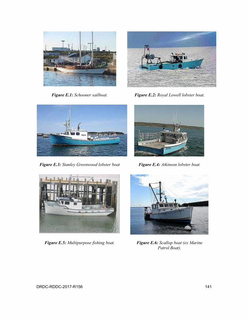
DRDC-RDDC-2017-R156 141
Figure E.1: Schooner sailboat. Figure E.2: Royal Lowell lobster boat.
Figure E.3: Stanley Greenwood lobster boat Figure E.4: Atkinson lobster boat.
Figure E.5: Multipurpose fishing boat. Figure E.6: Scallop boat (ex Marine Patrol Boat).
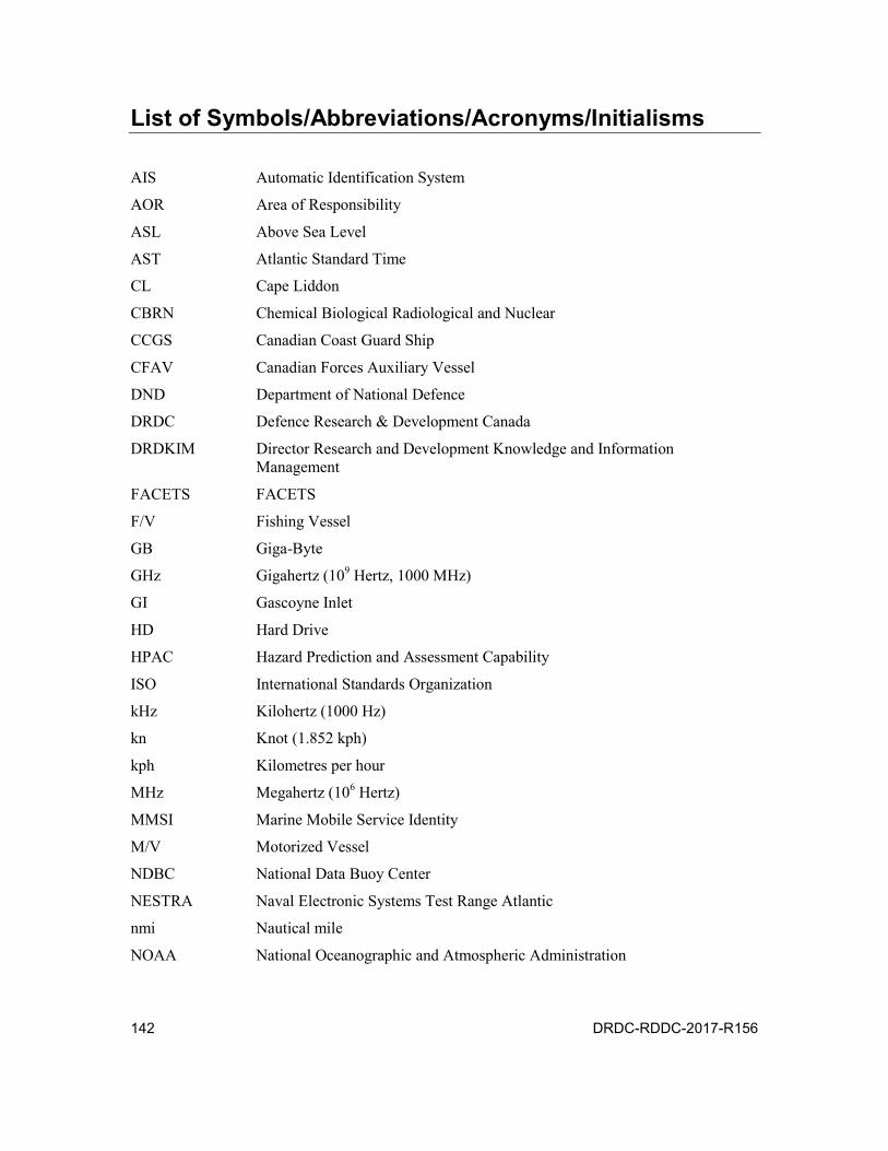
142 DRDC-RDDC-2017-R156
List of Symbols/Abbreviations/Acronyms/Initialisms
AIS Automatic Identification System
AOR Area of Responsibility
ASL Above Sea Level
AST Atlantic Standard Time
CL Cape Liddon
CBRN Chemical Biological Radiological and Nuclear
CCGS Canadian Coast Guard Ship
CFAV Canadian Forces Auxiliary Vessel
DND Department of National Defence
DRDC Defence Research & Development Canada
DRDKIM Director Research and Development Knowledge and Information Management
FACETS FACETS
F/V Fishing Vessel
GB Giga-Byte
GHz Gigahertz (109 Hertz, 1000 MHz)
GI Gascoyne Inlet
HD Hard Drive
HPAC Hazard Prediction and Assessment Capability
ISO International Standards Organization
kHz Kilohertz (1000 Hz)
kn Knot (1.852 kph)
kph Kilometres per hour
MHz Megahertz (106 Hertz)
MMSI Marine Mobile Service Identity
M/V Motorized Vessel
NDBC National Data Buoy Center
NESTRA Naval Electronic Systems Test Range Atlantic
nmi Nautical mile
NOAA National Oceanographic and Atmospheric Administration

DRDC-RDDC-2017-R156 143
NW Northern Watch
NWP Northwest Passage
RCMP Royal Canadian Mounted Police
RCS Radar Cross Section
R&D Research & Development
RHIB Rigid Hull Inflatable Boat
RMP Recognized Maritime Picture
RT Real-Time
RTE Radar Target Enhancer
R/V Research Vessel
SaR Search and Rescue
SAR Synthetic Aperture Radar
SATA Serial Advanced Technology Attachment
SIESTA Scenario (Shipborne) Integrated Environment for Tactics and Awareness
SS Sea State
S/V Sailing Vessel
TB Terabyte
UAV Unmanned Aerial Vehicle
UK United Kingdom
VOI Vessel of Interest
WUP watts-up? ProTM
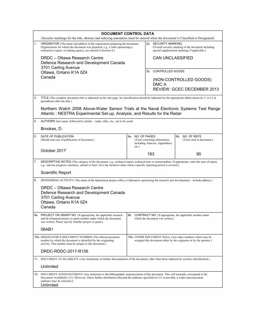
DOCUMENT CONTROL DATA (Security markings for the title, abstract and indexing annotation must be entered when the document is Classified or Designated)
1. ORIGINATOR (The name and address of the organization preparing the document. Organizations for whom the document was prepared, e.g., Centre sponsoring a contractor's report, or tasking agency, are entered in Section 8.) DRDC – Ottawa Research Centre Defence Research and Development Canada 3701 Carling Avenue Ottawa, Ontario K1A 0Z4 Canada
2a. SECURITY MARKING (Overall security marking of the document including special supplemental markings if applicable.)
CAN UNCLASSIFIED
2b. CONTROLLED GOODS
(NON-CONTROLLED GOODS) DMC A REVIEW: GCEC DECEMBER 2013
3. TITLE (The complete document title as indicated on the title page. Its classification should be indicated by the appropriate abbreviation (S, C or U) in
parentheses after the title.) Northern Watch 2008 Above-Water Sensor Trials at the Naval Electronic Systems Test Range Atlantic : NESTRA Experimental Set-up, Analysis, and Results for the Radar
4. AUTHORS (last name, followed by initials – ranks, titles, etc., not to be used) Brookes, D.
5. DATE OF PUBLICATION (Month and year of publication of document.) October 2017
6a. NO. OF PAGES (Total containing information, including Annexes, Appendices, etc.)
163
6b. NO. OF REFS (Total cited in document.)
90 7. DESCRIPTIVE NOTES (The category of the document, e.g., technical report, technical note or memorandum. If appropriate, enter the type of report,
e.g., interim, progress, summary, annual or final. Give the inclusive dates when a specific reporting period is covered.) Scientific Report
8. SPONSORING ACTIVITY (The name of the department project office or laboratory sponsoring the research and development – include address.) DRDC – Ottawa Research Centre Defence Research and Development Canada 3701 Carling Avenue Ottawa, Ontario K1A 0Z4 Canada
9a. PROJECT OR GRANT NO. (If appropriate, the applicable research and development project or grant number under which the document was written. Please specify whether project or grant.)
06AB1
9b. CONTRACT NO. (If appropriate, the applicable number under which the document was written.)
10a. ORIGINATOR’S DOCUMENT NUMBER (The official document number by which the document is identified by the originating activity. This number must be unique to this document.) DRDC-RDDC-2017-R156
10b. OTHER DOCUMENT NO(s). (Any other numbers which may be assigned this document either by the originator or by the sponsor.)
11. DOCUMENT AVAILABILITY (Any limitations on further dissemination of the document, other than those imposed by security classification.)
Unlimited
12. DOCUMENT ANNOUNCEMENT (Any limitation to the bibliographic announcement of this document. This will normally correspond to the Document Availability (11). However, where further distribution (beyond the audience specified in (11) is possible, a wider announcement audience may be selected.)) Unlimited
13. ABSTRACT (A brief and factual summary of the document. It may also appear elsewhere in the body of the document itself. It is highly desirable that the abstract of classified documents be unclassified. Each paragraph of the abstract shall begin with an indication of the security classification of the information in the paragraph (unless the document itself is unclassified) represented as (S), (C), (R), or (U). It is not necessary to include here abstracts in both official languages unless the text is bilingual.)
In August 2008 a team of scientists and technicians from DRDC attempted to undertake the first Arctic field trials for the Northern Watch Technology Demonstration Program (TDP) project on Devon Island at sites in Gascoyne Inlet and on Cape Liddon. Key objectives of the operation were to deploy several above water sensor (AWS) systems on Cape Liddon and an underwater sensor (UWS) system in Barrow Strait. The aim was to evaluate their individual and collective ability to detect, track, classify and identify a cooperative vessel, or targets of opportunity. Very severe weather prevented the accomplishment of this objective, so alternative trials were arranged for the AWS at the Naval Electronic Systems Test Range Atlantic (NESTRA) near Halifax in 7–11 Dec. 2008. The main intent was to perform a comprehensive shake down of all the AWS systems and perform as many of the original Arctic system tests as possible under the constraints imposed by this southern site. This report is one of several that are anticipated to result from the analyses of the NESTRA Trials data for each of the main AW sensors; this one is focused primarily on the performance of the navigation radar system. The results of the radar data analysis were generally consistent with performance predicted by the Scenario/Shipboard Integrated Environment for Tactics and Awareness (SIESTA) for the environmental conditions and the target-sensor geometries. The CFAV Quest was tracked to a maximum distance (stern-, or bow-on) about 29 km; large container vessels were tracked up to 35 km; and small vessels were tracked to distances of 10 to 20 km. The main factor limiting the radar’s ability to track ships was the line of sight to the horizon. The indications were that this radar system would be suitable for further evaluation at the arctic trials site near Gascoyne Inlet.
---------------------------------------------------------------------------------------------------------------
En août 2008, une équipe de scientifiques et de techniciens de RDDC a voulu mener en Arctique, plus précisément à Gascoyne Inlet et Cap Liddon, sur l’île Devon, les premiers essais sur le terrain du Projet de démonstration de technologies Surveillance du Nord (PDT NW). Cette opération visait principalement à déployer plusieurs systèmes de capteurs au-dessus de la surface (AWS) à Cap Liddon et un système de capteurs sous-marins (UWS) au détroit de Barrow, afin d’évaluer leur utilité collective et individuelle à détecter, poursuivre, classifier et identifier un navire ami ou des objectifs inopinés. Comme des conditions météorologiques extrêmes ont empêché d’atteindre cet objectif, on a plutôt tenu du 7 au 11 décembre 2008 des essais des systèmes AWS au Centre d’essai des systèmes électroniques naval de l’Atlantique (NESTRA), près d’Halifax. Ils ont surtout visé à faire des essais exhaustifs des systèmes AWS et de mener autant des tests prévus en environnement arctique que l’a permis ce site plus éloigné du pôle. Le présent rapport est le premier de plusieurs prévus sur les analyses des données des essais NESTRA visant chacun des principaux capteurs de surface, et il porte surtout sur les performances du système radar de navigation. Les résultats de cette analyse concordent en gros avec les performances prévues selon un scénario du système embarqué d’environnement intégré de tactique et de connaissance de la situation (SIESTA), dans les conditions environnementales et avec la configuration des cibles et des capteurs simulées. On a poursuivi le NAFC Quest jusqu’à une distance maximale de 29 km, de poupe ou de proue; des grand navires transporteurs de conteneurs, jusqu’à 35 km; et des navires plus petits, de 10 à 20 km. Le facteur déterminant dans la capacité de poursuite du radar s’est révélé être la visibilité jusqu’à la ligne d’horizon. Ces essais indiquent que ce système radar se prêterait bien à des essais plus poussés au site d’essai arctique près de Gascoyne Inlet.
14. KEYWORDS, DESCRIPTORS or IDENTIFIERS (Technically meaningful terms or short phrases that characterize a document and could be helpful in cataloguing the document. They should be selected so that no security classification is required. Identifiers, such as equipment model designation, trade name, military project code name, geographic location may also be included. If possible keywords should be selected from a published thesaurus, e.g., Thesaurus of Engineering and Scientific Terms (TEST) and that thesaurus identified. If it is not possible to select indexing terms which are Unclassified, the classification of each should be indicated as with the title.) radar; Arctic; sensor integration; sensor suite; Gascoyne Inlet; Cape Liddon; Northern Watch; Technology Demonstration Program; TDP; above-water sensors; AWS; underwater sensors; UWS; NESTRA; AIS; CANDISS; North Warning System