north field, qatar: a study of condensate blockage and...
TRANSCRIPT
North Field, Qatar: A Study of Condensate Blockage and Petroleum
Streams Management
M.Sc. Thesis
BY ARIF KUNTADI
SUPERVISOR: PROF. CURTIS H. WHITSON
Trondheim, June 2004
DEPARTMENT OF PETROLEUM ENGINEERING AND APPLIED GEOPHYSICS
NORWEGIAN UNIVERSITY OF SCIENCE AND TECHNOLOGY
North Field, Qatar: A Study of Condensate Blockage and Petroleum Streams Management
NTNU
Norges teknisk-naturvitenskapelige universitet
Fakultet for ingeniørvitenskap og teknologi Faculty of Engineering and Technology
Studieprogram i Geofag og petroleumsteknologi Study Programme in Earth Sciences and Petroleum Engineering
Institutt for petroleumsteknologi og anvendt geofysikk Department of Petroleum Engineering and Applied Geophysics
HOVEDOPPGAVEN/DIPLOMA THESIS/MASTER OF SCIENCE THESIS
Kandidatens navn/ The candidate’s name: ARIF KUNTADI Oppgavens tittel, engelsk/Title of Thesis, English: North Field, Qatar: A Study of Condensate Blockage and Petroleum Streams Management Utfyllende tekst/Extended text: This thesis aims to study the behaviour North Field gas condensate reservoir mainly in term of condensate blockage phenomenon near the wellbore which gives very significant well deliverability loss. Radial and Full Field reservoir model are simulated and some observations at the region near the wellbore have been done. Petroleum streams management has been developed for North Field to generate a complete compositional streams database. Studieretning/Area of specialization: Reservoir Engineering Fagområde/Combination of subjects: PVT, Reservoir Simulation and Petroleum
Streams Engineering Tidsrom/Time interval: January –June 2004
Faglærer/Teacher Original: Student Kopi: Fakultet Kopi: Institutt
M.Sc. Thesis, IPT, 2004 Page 2 of 125
North Field, Qatar: A Study of Condensate Blockage and Petroleum Streams Management
Acknowledgments I wish to express my sincerest gratitude to my supervisor Professor Curtis H. Whitson for his invaluable personal and academic guidance throughout the whole work of this thesis and also for his fresh ideas and insights when discussing every topic in this thesis. I especially thank to Dr. Mohammad Faiz ul Hoda and Dr. Knut Uleberg who helped me to develop petroleum streams management of North Field and with whom I had interesting discussions for improving the quality of this thesis. I also thank to QUOTA Programme for giving me financial support in two years studying at the Department of Petroleum Engineering and Applied Geophysics of the Norwegian University of Science and Technology. I would like to give my thanks to the office staffs at IPT, NTNU, and also all my friends for their cares and “smart” discussions in this latest two years. Finally, I would like to dedicate this thesis to my parents who always give me constant encouragement. I am indebted to my wife, Astri, who always be patient to stand by me and encourage me to finish my study and thesis. Last but not least, I am also indebted to my son, Akhtar, a “little star” who has been my new spirit to finish this thesis.
Trondheim, June 2004
Arif Kuntadi
M.Sc. Thesis, IPT, 2004 Page 3 of 125
North Field, Qatar: A Study of Condensate Blockage and Petroleum Streams Management
Table of Contents
ACKNOWLEDGMENTS.........................................................................................................3
TABLE OF CONTENTS ..........................................................................................................4
ABSTRACT ...............................................................................................................................6
1. INTRODUCTION .........................................................................................................7
2. EQUATION OF STATE (EOS) AND RESERVOIR MODEL ................................8 2.1. EOS MODEL.....................................................................................................................8 2.2. RESERVOIR MODEL ..........................................................................................................8
3. CONDENSATE BLOCKAGE PHENOMENON.....................................................10
3.1. INTRODUCTION ...............................................................................................................10 3.2. GAS CONDENSATE RATE EQUATION ................................................................................10
3.2.1. Flow Regions .........................................................................................................11 3.2.2. Calculating Pseudopressure..................................................................................11
3.3. RELATIVE PERMEABILITY NEAR WELLBORE....................................................................13 3.4. RELATIVE PERMEABILITY IN KHUFF FORMATION............................................................14
4. RADIAL MODEL SIMULATION ............................................................................17 4.1. RESERVOIR MODEL DESCRIPTION....................................................................................17
4.1.1. Gridding and Layering ..........................................................................................17 4.1.2. Permeability distribution.......................................................................................17
4.2. RADIAL MODEL SIMULATION AND RESULTS ..................................................................18 4.3. OBSERVATION AT AREA NEAR WELL BORE......................................................................18
4.3.1. Gas Rate distribution.............................................................................................18 4.3.2. Capillary number profile .......................................................................................19 4.3.3. Oil Gas Ratio (OGR) profile .................................................................................19 4.3.4. Oil Saturation profile ............................................................................................19 4.3.5. Correlations...........................................................................................................19 4.3.6. Permeability Effect ................................................................................................20
5. SKIN FACTOR PREDICTION.................................................................................23
5.1. CONDENSATE SKIN FACTOR PREDICTION ........................................................................23 5.2. EFFECTIVE SKIN FACTOR PREDICTION.............................................................................25
6. SENSITIVITY ANALYSIS ........................................................................................27
6.1. COREY-LIKE EQUATION EXPONENT AND PRODUCTION TUBING SIZE...............................27 6.2. PRESSURE CONSTRAINTS AND TUBING SIZE ...................................................................27 6.3. PERMEABILITY DISTRIBUTION.........................................................................................28
6.3.1. Radial Model Simulation.......................................................................................28 6.3.2. Full Field Model Simulation .................................................................................28
7. PETROLEUM STREAM MANAGEMENT ............................................................30
7.1. PETROLEUM STREAMS MANAGEMENT IN NORTH FIELD..................................................30 7.2. GENERATING STREAMS DATABASE OF NORTH FIELD......................................................32
M.Sc. Thesis, IPT, 2004 Page 4 of 125

North Field, Qatar: A Study of Condensate Blockage and Petroleum Streams Management
7.3. SOME APPLICATIONS IN STREAMS DATABASE .................................................................33
8. CONCLUSIONS..........................................................................................................35
NOMENCLATURE ................................................................................................................36
REFERENCES ........................................................................................................................39
TABLES ...................................................................................................................................40
FIGURES .................................................................................................................................47
APPENDIX A.........................................................................................................................106 1. FULL FIELD RESERVOIR MODEL DATASET ...................................................................106 2. RADIAL RESERVOIR MODEL DATASET .........................................................................112
APPENDIX B.........................................................................................................................119 1. EXTRACT OF MAIN STREAM FILE WHICH IS CONVERTED FROM THE SIMULATION RESULT
STREAMS.......................................................................................................................119 2. EXTRACT OF WELL STREAM FILES WHICH IS THE RESULT OF FILTERING OPERATION OF
MAIN STREAM FILE.......................................................................................................120 3. EXTRACT OF AVERAGE WELL STREAM FILES WHICH IS THE RESULT OF AGGREGATION AND
AVERAGING OPERATIONS OF WELL STREAM FILE. .........................................................121 4. EXTRACT OF AVERAGE WELL LAYER STREAM FILES WHICH IS THE RESULT OF
AGGREGATION AND AVERAGING OPERATIONS OF WELL LAYER STREAM FILE. ..............122
APPENDIX C.........................................................................................................................123 1. SPREADSHEET CALCULATION EXAMPLE FOR PREDICTING THE GAS RATE WITH EXCLUDING
AND INCLUDING THE CAPILLARY NUMBER EFFECT........................................................123 2. SPREADSHEET CALCULATION EXAMPLE FOR PREDICTING THE DRY GAS RATE ..............123
M.Sc. Thesis, IPT, 2004 Page 5 of 125
North Field, Qatar: A Study of Condensate Blockage and Petroleum Streams Management
Abstract North Field is a giant gas condensate reservoir in Qatar which has estimated gas reserves more than 900 Tcf. This field is a part of Khuff formation and has four main productive layers: K1, K2, K3 and K4. The main objectives of this thesis are to study the condensate blockage phenomenon in this reservoir and to develop petroleum streams management procedures for given production line structure. This thesis uses an Equation of State (EOS) model and reservoir model which have been developed previously3. The developed EOS model was a Soave-Redlich-Kwong (SRK) EOS with 24 components. The developed reservoir model was a full field Cartesian model, no communication layering system between geological layers, uniform porosity and permeability in each geological layer and produced by 20 wells. A radial well model is developed as a representation of one production well in the full field reservoir model. This model then is run for different permeability distributions to study the effect of condensate blockage. Near well region observations have been made specifically for gas rate, oil saturation, producing OGR and capillary number profiles. Observation in the log normal permeability distribution model simulation shows that there are some correlations between capillary number, oil saturation and producing OGR at the near-well region. The very low permeability model gives higher producing OGR and oil saturation compared than the moderate low model (the original model). In both permeability models the capillary number is proportional to the production gas rate. Another observation result from the radial model simulation shows that most well deliverability loss happens in the region near the wellbore where both gas and condensate are flowing. The krg dramatically drops in this region due to condensate banking. The ratio krg/kro(P) and krg(krg/kro) are the most important parameter to describe the phenomena in this region. The krg/kro(P) can be predicted by PVT simulation of the developed EOS model. Both PVT simulation and reservoir simulation give the same range of this parameter from 1 – 100. This thesis demonstrates how to use the spreadsheet calculation to accurately reproduce the gas production rate of the radial simulation model when the produced GOR is given. The condensate blockage skin factor is also able to be predicted by this hand-calculation. The effective skin factor which represents the condensate blockage effect in the full field model simulation is predicted by matching the full field simulation to the radial model simulation. This matching gives effective skin factor ranges from 3 (for high capillary number) to 15 (not including capillary number effect). This range is independent of the permeability distribution. Some sensitivity analyses have been done to see the effect of permeability distribution, capillary number and tubing size in the simulation of North Field. The capillary number gives significant improvement of the gas production plateau period when simulated in the very low permeability model but it doesn’t for moderate low permeability model. Log normal and uniform permeability model give almost identical simulation result. Petroleum streams management has been developed by performing some sequences to generate the streams database from the simulation output file for one block concession of North Field. The streams database gives a complete description of the streams in all production nodes of the model and could be used to perform a reservoir production optimization. Some plots are generated to show the usefulness of the developed streams database. All data used in this thesis was based directly or founded on information in the public domain. Complete references are given at the end of this thesis.
M.Sc. Thesis, IPT, 2004 Page 6 of 125
North Field, Qatar: A Study of Condensate Blockage and Petroleum Streams Management
1. Introduction North Field, firstly discovered in 1971, is situated just offshore to the North East of the peninsular landmass of Qatar as shown in Fig. 1 and, geologically, in communication with Iran's South Pars. North Field has gas reserves estimated more than 900 Tcf and considered as the world's second largest holder of gas reserves after Russia or the largest single gas field in the world. This field covers an area of more than 6000 square kilometers which is nearly half the size of Qatar land. North Field reservoir which is a part of Permian Khuff formation mainly consists of mixture of dolomite and limestone and has 4 geological layers (starting from the top): K1, K2, K3 and K48.
Previous work3 developed an Equation of State (EOS) model and reservoir model for North Field. In the following chapter there will be a brief description about the developed EOS model and full field reservoir model. Condensate blockage phenomenon in the near-wellbore can be important issue in the deliverability of a gas condensate reservoir. This phenomenon significantly reduces the well deliverability and for a given pressure constraint (e.g. bottom hole flowing pressure) it gives reductions in the recovery both of gas and condensate accordingly. The radial model with single production well and fine grid is run to capture the effect of condensate banking in the near-wellbore during the field production life. The log normal distribution model of permeability is introduced to study the effect on gas rate, capillary number, oil gas ratio (OGR) and oil saturation at the first radial block. The very low and uniform permeability model is also run and then compared to the log normal model. Fevang and Whitson1 described how significant the ratio krg/kro in the region near the wellbore is. They mentioned that by being given an accurate OGR it is possible to reproduce the gas rate almost exact as the gas rate which was produced from the radial and fine grid model simulation. This thesis work will demonstrate how the spreadsheet calculation is able to reproduce the simulation gas rate for a given OGR and predict the condensate blockage skin factor. The full field model (FFM) which has been developed in the previous work has a coarse grid model that can not capture the condensate banking near the wellbore. To include this near well phenomenon it needs to put some skin factor in the FFM which then makes the FFM simulation behaves like the radial model simulation. The procedures to match FFM wells to a fine gridded radial model will also be discussed in this thesis. In the sensitivity analysis there will be discussions about some parameters which are considered important factors to understand the behavior of a gas condensate reservoir. Corey-like exponents, production tubing size, pressure constraints and permeability distribution have been examined. Petroleum streams management is basically not only important to study in gas condensate reservoir, but in gas condensate reservoir the compositional streams are more valuable than in oil reservoir because the compositional streams determine how much the part of the produced reservoir fluids will be as natural gas or Liquefied Natural Gas (LNG), Liquefied Petroleum Gas (LPG) and as condensate. This thesis work has developed an early step of a complicated petroleum stream management of North Field, Qatar. A further study is still needed to be done to develop a comprehensive petroleum streams management in such huge gas condensate reservoir.
M.Sc. Thesis, IPT, 2004 Page 7 of 125
North Field, Qatar: A Study of Condensate Blockage and Petroleum Streams Management
2. Equation of State (EOS) and Reservoir Model Cubic equations of state (EOS’s) are simple equations relating pressure, volume, and temperature (PVT). They accurately describe the volumetric and phase behavior of pure compounds and mixtures, requiring only critical properties and acentric factor of each component. The same equation is used to calculate the properties of all phases, thereby ensuring consistency in reservoir processes that approach critical conditions (e.g., miscible-gas injection and depletion of volatile-oil/gas-condensate reservoirs). Problems involving multiphase behavior, such as low-temperature CO2 flooding, can be treated with an EOS, and even water-/hydrocarbon-phase behavior can be predicted accurately with a cubic EOS13. Due to its huge gas reserves so an appropriate development of North Field is needed to be done carefully in order the gas reserves which have been discovered in this field could be recovered optimally. One of the tools usually used in petroleum engineering to give comprehensive evaluation of the potentiality of the reservoir is reservoir simulation. Simulation will give accurate result if uses an accurate description of the reservoir fluid phase behavior and the appropriate reservoir model. This chapter gives the description about the EOS model and the full field reservoir model which have been developed in Ref. 3.
2.1. EOS Model Almarry and Al-Saadoon6 developed an EOS model for North Field fluids, particularly for K4 formation fluids. They used the Peng Robinson (PR) EOS model but unfortunately they did not provide the detail component properties of their model. The new EOS model was developed with SRK EOS as described in Ref. 3. SPE 13715 only provided the composition of original reservoir fluids which dealing with single carbon number up to C6 and one heaviest fraction of C7+. This heaviest fraction was characterized by Gamma distribution model to get 13 new components with the heaviest components C30+. The developed SRK EOS model had 24 components which then it was named SRK EOS24. Ref. 3 discussed the procedure to characterize the C7+ fraction using PhazeComp and it also explained the way to match this SRK EOS24 model to some experiment data which were obtained from SPE 13175. Fig. 2 - Fig. 3 show the agreements between the CVD experiments data and what the SRK EOS24 model predicted. The final SRK EOS24 model parameters resulted from C7+ fraction characterization and EOS model matching are presented in Table 1 and its complete BIPs are presented in Table 2. The SRK EOS24 model was developed from the reservoir fluid properties of K4 formation but then it was also used to model the reservoir fluid of the other three formations: K1, K2 and K3. Some papers8,9 mentioned that K2 and K3 have H2S contents slightly higher than K4 so the difference then only at initial composition of K2/K3 and K4, still can use the same EOS model. The reservoir fluid of K1 is basically similar to K4. The calculated initial gas compositions of North Field’s fluids are presented in Table 3.
2.2. Reservoir Model The full field reservoir model (FFM) which was developed in Ref. 3 only modeled one block concession of North Field since it is really needed numerous grid blocks to model the whole area which covers more than 6000 sq km. The FFM covers the area of 100 sq km or equivalent to 10 km x 10 km. Both the previous work and this thesis work use the free version of Sensor simulator which has maximum active grid blocks of 6000. The North Field FFM was a grid coarse Cartesian model with DX = DY = 500 m. The geological layers K1, K2 and K3 were divided into 3 numerical layers each and then K4 was
M.Sc. Thesis, IPT, 2004 Page 8 of 125
North Field, Qatar: A Study of Condensate Blockage and Petroleum Streams Management
divided into 4 numerical layers. So finally the reservoir model had dimension of 20 x 20 x 17 including the 3 seal layers between each geological layer and one bottom seal layer. The final layering model of North Field (Khuff formation) is presented in Fig. 4. Al-Shiddiqi and Dawe8 explained that this formation has porosity ranging from 4–20%, and average permeability of 30 md. They also described that the permeability of K2/K3 ranging from 3 – 1800 md and K1/K4 have somewhat lower permeability. The FFM used permeability of 45 md for K2/K3 and 15 md for K1/K4. It used uniform porosity for each geological layer which were 10% for K1/K4 and 15% for K2/K3. The vertical permeability used was 10% of the horizontal permeability. The analytical relative permeability correlation used was a Corey-like equation. Detail formation properties and relative permeability correlation parameters are presented in Table 4. As previously discussed, the PVT properties used in the FFM were the SRK EOS24 model with two different initial gas compositions of K1/K4 and K2/K3. Since the FFM had 2 different initial gas composition then it was initialized by two different initialization regions, one was for K1/K4 and the other was for K2/K3. The gas plateau rate was set at 2000 MMSCF/D with 20 production wells which means each well producing 100 MMSCF/D. The wells positions are shown at Fig. 5 and all wells were perforated in all numerical layers. Detail description of the North Field FFM is presented at Table 4.
M.Sc. Thesis, IPT, 2004 Page 9 of 125

North Field, Qatar: A Study of Condensate Blockage and Petroleum Streams Management
3. Condensate Blockage Phenomenon
3.1. Introduction The typical chemical composition of a gas-condensate mixture is dominated by volatile components such as methane, and a rather ‘small’ amount of heavy hydrocarbon components (<15 mol-%), though these heavier components make up a considerably larger percentage of the liquid phase (‘retrograde condensate’) formed during pressure decrease below an upper dew point. For practically any retrograde condensate reservoir, the condensate saturation is, throughout most of the reservoir, so low that its mobility is much less than gas mobility and for practical purposes can be considered immobile. Nevertheless, this gas-dominated flow behavior is not correct in the near-well vicinity where condensate saturations often reach high values (>50%), and oil permeability may exceed gas permeability (krg/kro< 1)2. Condensate blockage near the wellbore may reduce gas well deliverability appreciably, though the severity depends on a number of reservoir and well parameters. Condensate blockage is important if the pressure drop from the reservoir to the wellbore is a significant percentage of the total pressure drop from reservoir to delivery point (e.g. a surface separator) at the time (and after) a well goes on decline. Reservoirs with low-to-moderate permeability (<10–50 md) are often ‘problem’ wells where condensate blockage must be handled properly. Wells with high kh products (>5–10,000 md-ft) are typically not affected by reservoir pressure drop because the well’s deliverability is constrained almost entirely by the tubing. In this case, condensate blockage is a non-issue2.
3.2. Gas condensate rate equation The general volumetric rate equation for a gas condensate well of any geometry (e.g. radial, vertically fractured, or horizontal) is, for a compositional formulation,
PR g rgSC o rog S Pwf
o o g gSC
kRT kq C dP M M
ρρβµ µ
⎛ ⎞⎛ ⎞ ⎛ ⎞⎜ ⎟⎜ ⎟ ⎜ ⎟⎜ ⎟ ⎜ ⎟⎝ ⎠⎝ ⎠ ⎝ ⎠
= +∫ p .............................................................................. (1)
or in terms of black-oil PVT,
s
PR rgrog Pwf
o o ggdR
kkq C dB Bµ µ
⎛ ⎞⎛ ⎞⎜ ⎟⎜ ⎟ ⎜ ⎟⎝ ⎠ ⎝ ⎠
= +∫ p ..................................................................................................(2)
where
( )12
ln / 0.75e w
a khr r s
C π− +
= ........................................................................................................(3)
a1=1/(2π 141.2) for field units, and a1=1 for pure SI units. The constant C includes basic reservoir properties such as permeability k, thickness h, drainage radius re, wellbore radius rw, and other constants. Skin s is a composite factor that includes non-ideal flow effects such as damage, stimulation, drainage geometry, and partial penetration. Fevang and Whitson1 mentioned that relative permeabilities krg and kro are defined relative to absolute permeability, and not relative to permeability at irreducible water saturation.
M.Sc. Thesis, IPT, 2004 Page 10 of 125
North Field, Qatar: A Study of Condensate Blockage and Petroleum Streams Management
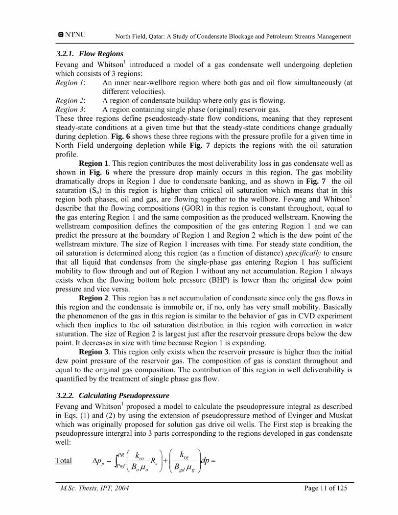
3.2.1. Flow Regions Fevang and Whitson1 introduced a model of a gas condensate well undergoing depletion which consists of 3 regions: Region 1: An inner near-wellbore region where both gas and oil flow simultaneously (at
different velocities). Region 2: A region of condensate buildup where only gas is flowing. Region 3: A region containing single phase (original) reservoir gas. These three regions define pseudosteady-state flow conditions, meaning that they represent steady-state conditions at a given time but that the steady-state conditions change gradually during depletion. Fig. 6 shows these three regions with the pressure profile for a given time in North Field undergoing depletion while Fig. 7 depicts the regions with the oil saturation profile. Region 1. This region contributes the most deliverability loss in gas condensate well as shown in Fig. 6 where the pressure drop mainly occurs in this region. The gas mobility dramatically drops in Region 1 due to condensate banking, and as shown in Fig. 7 the oil saturation (So) in this region is higher than critical oil saturation which means that in this region both phases, oil and gas, are flowing together to the wellbore. Fevang and Whitson1 describe that the flowing compositions (GOR) in this region is constant throughout, equal to the gas entering Region 1 and the same composition as the produced wellstream. Knowing the wellstream composition defines the composition of the gas entering Region 1 and we can predict the pressure at the boundary of Region 1 and Region 2 which is the dew point of the wellstream mixture. The size of Region 1 increases with time. For steady state condition, the oil saturation is determined along this region (as a function of distance) specifically to ensure that all liquid that condenses from the single-phase gas entering Region 1 has sufficient mobility to flow through and out of Region 1 without any net accumulation. Region 1 always exists when the flowing bottom hole pressure (BHP) is lower than the original dew point pressure and vice versa. Region 2. This region has a net accumulation of condensate since only the gas flows in this region and the condensate is immobile or, if no, only has very small mobility. Basically the phenomenon of the gas in this region is similar to the behavior of gas in CVD experiment which then implies to the oil saturation distribution in this region with correction in water saturation. The size of Region 2 is largest just after the reservoir pressure drops below the dew point. It decreases in size with time because Region 1 is expanding. Region 3. This region only exists when the reservoir pressure is higher than the initial dew point pressure of the reservoir gas. The composition of gas is constant throughout and equal to the original gas composition. The contribution of this region in well deliverability is quantified by the treatment of single phase gas flow.
3.2.2. Calculating Pseudopressure Fevang and Whitson1 proposed a model to calculate the pseudopressure integral as described in Eqs. (1) and (2) by using the extension of pseudopressure method of Evinger and Muskat which was originally proposed for solution gas drive oil wells. The First step is breaking the pseudopressure intergral into 3 parts corresponding to the regions developed in gas condensate well:
Total p s
PR rgroPwf
o o ggdp R
kk dpB Bµ µ
⎛ ⎞⎛ ⎞∆ =⎜ ⎟⎜ ⎟ ⎜ ⎟⎝ ⎠ ⎝ ⎠
= +∫
M.Sc. Thesis, IPT, 2004 Page 11 of 125
North Field, Qatar: A Study of Condensate Blockage and Petroleum Streams Management
Region 1 *
s
P rgroPwf
o o ggdR
kk dpB Bµ µ
⎛ ⎞⎛ ⎞+⎜ ⎟⎜ ⎟ ⎜ ⎟⎝ ⎠ ⎝ ⎠
+∫
Region 2 *
Pd rg
Pggd
kdp
B µ+∫
Region 3 ( ) 1rg wi
PR
Pdggd
k S dpB µ∫ .........................................................................................(4)
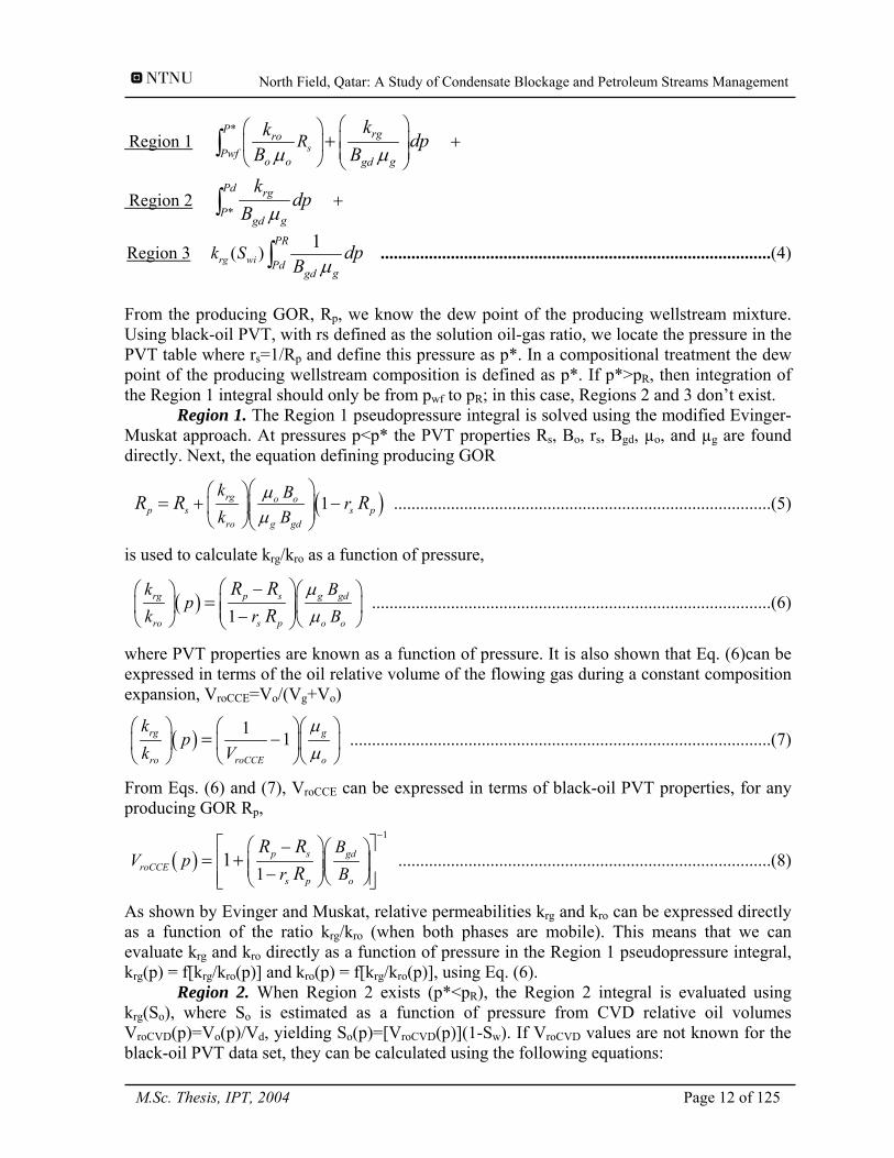
From the producing GOR, Rp, we know the dew point of the producing wellstream mixture. Using black-oil PVT, with rs defined as the solution oil-gas ratio, we locate the pressure in the PVT table where rs=1/Rp and define this pressure as p*. In a compositional treatment the dew point of the producing wellstream composition is defined as p*. If p*>pR, then integration of the Region 1 integral should only be from pwf to pR; in this case, Regions 2 and 3 don’t exist.
Region 1. The Region 1 pseudopressure integral is solved using the modified Evinger-Muskat approach. At pressures p<p* the PVT properties Rs, Bo, rs, Bgd, µo, and µg are found directly. Next, the equation defining producing GOR
(1rg o op s s p
ro g gd
k B rk B
R R Rµµ
⎛ ⎞⎛ ⎞+ ⎜ ⎟⎜ ⎟⎜ ⎟⎝ ⎠⎝ ⎠
= )− ......................................................................................(5)
is used to calculate krg/kro as a function of pressure,
( )1
rg p s g gd
ro s p o o
k Bp
k rR R
Rµµ
⎛ ⎞−⎛ ⎞ ⎛⎜ ⎟⎜ ⎟ ⎜⎜ ⎟−⎝ ⎠ ⎝⎝ ⎠
=B
⎞⎟⎠
...........................................................................................(6)
where PVT properties are known as a function of pressure. It is also shown that Eq. (6)can be expressed in terms of the oil relative volume of the flowing gas during a constant composition expansion, VroCCE=Vo/(Vg+Vo)
( ) 1 1rg g
ro roCCE o
kp
k Vµµ
⎛ ⎞ ⎛ ⎞⎛−⎜ ⎟ ⎜ ⎟⎜
⎝ ⎠ ⎝ ⎠⎝=
⎞⎟⎠
................................................................................................(7)
From Eqs. (6) and (7), VroCCE can be expressed in terms of black-oil PVT properties, for any producing GOR Rp,
( )1
11 p s gd
roCCEs p o
BV p
r BR R
R
−⎡ ⎤⎛ ⎞− ⎛ ⎞⎢ ⎜ ⎟⎜ ⎟⎜ ⎟−⎢ ⎥⎝ ⎠⎝ ⎠⎣ ⎦
= + ⎥ .....................................................................................(8)
As shown by Evinger and Muskat, relative permeabilities krg and kro can be expressed directly as a function of the ratio krg/kro (when both phases are mobile). This means that we can evaluate krg and kro directly as a function of pressure in the Region 1 pseudopressure integral, krg(p) = f[krg/kro(p)] and kro(p) = f[krg/kro(p)], using Eq. (6).
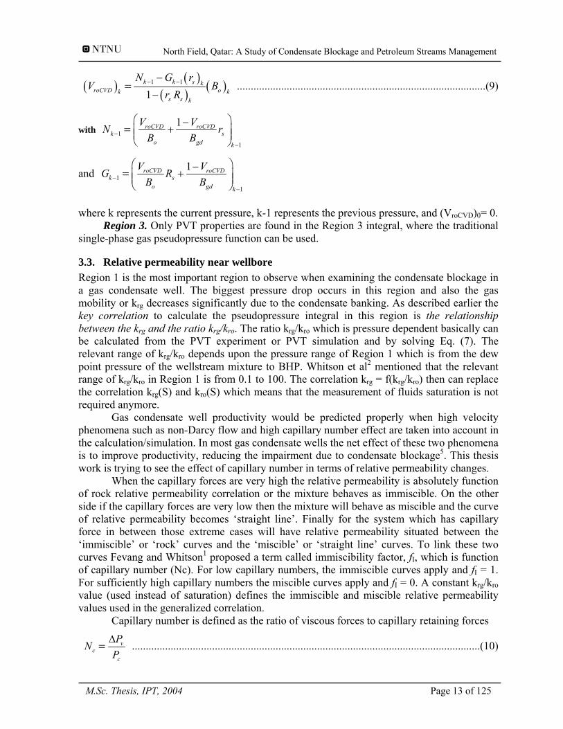
Region 2. When Region 2 exists (p*<pR), the Region 2 integral is evaluated using krg(So), where So is estimated as a function of pressure from CVD relative oil volumes VroCVD(p)=Vo(p)/Vd, yielding So(p)=[VroCVD(p)](1-Sw). If VroCVD values are not known for the black-oil PVT data set, they can be calculated using the following equations:
M.Sc. Thesis, IPT, 2004 Page 12 of 125
North Field, Qatar: A Study of Condensate Blockage and Petroleum Streams Management
( ) ( )( ) ( )1 1
1k k s k
roCVD oks s k
N G rV
r R− −−
−=
kB ..........................................................................................(9)
with 1
1
1roCVD roCVDk s
o gd k
V VN rB B−
−
⎛ ⎞−+⎜ ⎟⎜ ⎟
⎝ ⎠=
and 1
1
1roCVD roCVDk s
o gd k
V VG RB B−
−
⎛ ⎞−+⎜ ⎟⎜ ⎟
⎝ ⎠=
where k represents the current pressure, k-1 represents the previous pressure, and (VroCVD)0= 0.
Region 3. Only PVT properties are found in the Region 3 integral, where the traditional single-phase gas pseudopressure function can be used.
3.3. Relative permeability near wellbore Region 1 is the most important region to observe when examining the condensate blockage in a gas condensate well. The biggest pressure drop occurs in this region and also the gas mobility or krg decreases significantly due to the condensate banking. As described earlier the key correlation to calculate the pseudopressure integral in this region is the relationship between the krg and the ratio krg/kro. The ratio krg/kro which is pressure dependent basically can be calculated from the PVT experiment or PVT simulation and by solving Eq. (7). The relevant range of krg/kro depends upon the pressure range of Region 1 which is from the dew point pressure of the wellstream mixture to BHP. Whitson et al2 mentioned that the relevant range of krg/kro in Region 1 is from 0.1 to 100. The correlation krg = f(krg/kro) then can replace the correlation krg(S) and kro(S) which means that the measurement of fluids saturation is not required anymore. Gas condensate well productivity would be predicted properly when high velocity phenomena such as non-Darcy flow and high capillary number effect are taken into account in the calculation/simulation. In most gas condensate wells the net effect of these two phenomena is to improve productivity, reducing the impairment due to condensate blockage5. This thesis work is trying to see the effect of capillary number in terms of relative permeability changes. When the capillary forces are very high the relative permeability is absolutely function of rock relative permeability correlation or the mixture behaves as immiscible. On the other side if the capillary forces are very low then the mixture will behave as miscible and the curve of relative permeability becomes ‘straight line’. Finally for the system which has capillary force in between those extreme cases will have relative permeability situated between the ‘immiscible’ or ‘rock’ curves and the ‘miscible’ or ‘straight line’ curves. To link these two curves Fevang and Whitson1 proposed a term called immiscibility factor, fI, which is function of capillary number (Nc). For low capillary numbers, the immiscible curves apply and fI = 1. For sufficiently high capillary numbers the miscible curves apply and fI = 0. A constant krg/kro value (used instead of saturation) defines the immiscible and miscible relative permeability values used in the generalized correlation.
Capillary number is defined as the ratio of viscous forces to capillary retaining forces
vc
c
PNP∆= ..............................................................................................................................(10)
M.Sc. Thesis, IPT, 2004 Page 13 of 125
North Field, Qatar: A Study of Condensate Blockage and Petroleum Streams Management
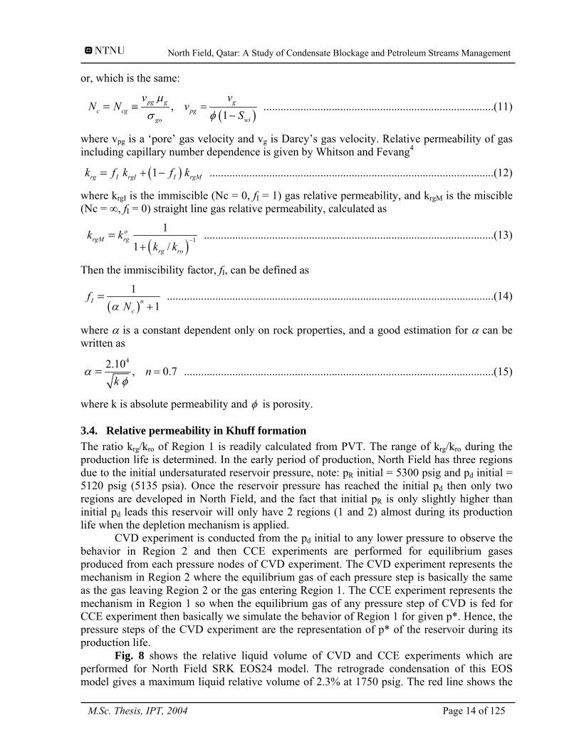
or, which is the same:
( ),
1pg g g
c cg pggo w
v vN N v
S i
µσ φ
≡ =−
= .................................................................................(11)
where vpg is a ‘pore’ gas velocity and vg is Darcy’s gas velocity. Relative permeability of gas including capillary number dependence is given by Whitson and Fevang4
( )1rg I rgI I rgMk f k f k+ −= ....................................................................................................(12)
where krgI is the immiscible (Nc = 0, fI = 1) gas relative permeability, and krgM is the miscible (Nc = ∞, fI = 0) straight line gas relative permeability, calculated as
( ) 1
1
1 /o
rgM rg
rg ro
k kk k
−+
= ......................................................................................................(13)
Then the immiscibility factor, fI, can be defined as
( )1
1I n
c
fNα +
= ...................................................................................................................(14)
where α is a constant dependent only on rock properties, and a good estimation for α can be written as
42.10 , 0nk
αφ
== .7 .............................................................................................................(15)
where k is absolute permeability and φ is porosity.
3.4. Relative permeability in Khuff formation The ratio krg/kro of Region 1 is readily calculated from PVT. The range of krg/kro during the production life is determined. In the early period of production, North Field has three regions due to the initial undersaturated reservoir pressure, note: pR initial = 5300 psig and pd initial = 5120 psig (5135 psia). Once the reservoir pressure has reached the initial pd then only two regions are developed in North Field, and the fact that initial pR is only slightly higher than initial pd leads this reservoir will only have 2 regions (1 and 2) almost during its production life when the depletion mechanism is applied. CVD experiment is conducted from the pd initial to any lower pressure to observe the behavior in Region 2 and then CCE experiments are performed for equilibrium gases produced from each pressure nodes of CVD experiment. The CVD experiment represents the mechanism in Region 2 where the equilibrium gas of each pressure step is basically the same as the gas leaving Region 2 or the gas entering Region 1. The CCE experiment represents the mechanism in Region 1 so when the equilibrium gas of any pressure step of CVD is fed for CCE experiment then basically we simulate the behavior of Region 1 for given p*. Hence, the pressure steps of the CVD experiment are the representation of p* of the reservoir during its production life. Fig. 8 shows the relative liquid volume of CVD and CCE experiments which are performed for North Field SRK EOS24 model. The retrograde condensation of this EOS model gives a maximum liquid relative volume of 2.3% at 1750 psig. The red line shows the
M.Sc. Thesis, IPT, 2004 Page 14 of 125

North Field, Qatar: A Study of Condensate Blockage and Petroleum Streams Management
behavior in Region 1 when pR is equal to pd initial or the first time in the production history when only 2 regions are developed in this reservoir. This plot gives us the maximum liquid relative volume of 1.5% at 2750 psig. The relevant range of fluids behavior in Region 1 depends upon how high the pressure constraint we put as the BHP is. The behavior of flowing reservoir fluids in Region 1 for p* lower than pd initial are represented by the others CCE relative liquid volume plots. Eq. (7) is used to calculate the relative permeability ratio krg/kro, Fig. 9 shows the range of krg/kro for the whole production life of Khuff formation. It is seen that the relevant range of krg/kro is from 2 – 100. There are some krg/kro higher than 100 but these occur for very low p*s. The p* of 1750 psig or lower practically only happens in the late of reservoir production history or under depletion production scenario it is the period when the reservoir could not produce the plateau production rate any longer (note: in the original scenario of this thesis the plateau rate is set at 100 MMSCF/D/well). The developed reservoir model of North Field applied analytical permeability correlation. The Corey-like correlation which is used in Sensor simulator is described below
11
nog
org wi gorog rocw
org wi
S S Sk k
S S⎛ ⎞− − −⎜⎜ − −⎝ ⎠
= ⎟⎟ ........................................................................................(16)
1
ng
g gcorg rgro
org gc wi
S Sk k
S S S⎛ ⎞−⎜⎜ − − −⎝ ⎠
= ⎟⎟ ..........................................................................................(17)
11
nowo orw w
row rocworw wi
S Sk kS S
⎛ ⎞− −⎜ − −⎝ ⎠
= ⎟ ...............................................................................................(18)
1
nwo w wi
rw rwroorw wi
S Sk kS S
⎛ ⎞−⎜ − −⎝ ⎠
= ⎟ .................................................................................................(19)
The correlation parameters used are presented in Table 4. This model uses exponent nog=no=3; the exponent parameter (n) basically affects the curvature of the plot of saturation vs. relative permeability; n=1 gives a ‘straight line’ correlation and the higher exponent (e.g. 3 or 4) have significant curvature. Exponent equal to 1.5 could be considered as the representation of relative permeability model for a system which has high capillary number and the infinity capillary number is represented by exponent 1. Fig. 10 shows the relative permeability vs. gas saturation of the developed model (n=3) and the representation of high capillary number model (n=1.5), while Fig. 11 depicts the relationship between krg vs. krg/kro for both models. Simple 1D radial model simulation with a single well has been done for Layer K4 to see the condensate blockage effect in Khuff formation in general. The results of the simulation are shown in Fig. 12 - Fig. 15. Again, it is clearly seen in Fig. 12 that the most pressure drop occurs in the region near the wellbore (Region 1) and three regions exist in early production period (40 days) where pR > 5135 psia (pd initial) and afterward only two regions (1 and 2) exist in the reservoir. The exact boundary of Region 1 and Region 2 is predicted by calculating the dew point of producing wellstream (p*) at a given time, but one quick way to locate this position is by pointing out where the oil start flowing or when So is already higher than Soc (Soc=20%). Fig. 13 shows that these boundaries are located at around 10 ft from the wellbore
M.Sc. Thesis, IPT, 2004 Page 15 of 125
North Field, Qatar: A Study of Condensate Blockage and Petroleum Streams Management
after 40 days simulation and around 50 ft after 500 days. It means that Region 1 is expanding by time and Region 2 is reducing accordingly. Fig. 15 also gives indication that the position where condensate begins being mobile is getting farther from the wellbore. Fig. 14 tells us how big the krg drops when gas flows near the wellbore, this is the key reason explaining why Region 1 contributes the most productivity loss in gas condensate well production history. This figure also shows that in Region 1 the relevant range of krg is 0.05 - 0.2 and then if we confirm this krg range to Fig. 11 we will get the ratio krg/kro situated from 1 – 100. This range of krg/kro, which is calculated from radial simulation, is very close to the range predicted from PVT simulation. This agreement becomes the evidence that the most relevant range of krg/kro in practical is from 1 – 100.
M.Sc. Thesis, IPT, 2004 Page 16 of 125
North Field, Qatar: A Study of Condensate Blockage and Petroleum Streams Management
4. Radial Model Simulation The fine grid model is required to study condensate blockage phenomenon in gas condensate reservoir. Radial reservoir model with one production well in the center is the suitable reservoir model when fine grid is needed. Basically full field model is still able to use to capture the condensate blockage effect but it needs to have local grid refinement in the area near the production wells. This thesis work has developed a radial model for North Field and then simulated this model to observe some phenomena near wellbore such as oil saturation, capillary number, oil gas ratio, and production gas rate.
4.1. Reservoir model description The main purpose of developing the radial model in this thesis work is to study gas condensate reservoir behavior in appropriate way which then its result could be taken into account in the FFM. The developed radial model is a representation of one production well in the FFM where the volumetric drainage used in radial model is equal to 1/20 of the FFM volumetric drainage. All the parameters used in the radial model are the same as the FFM except the gridding, layering and permeability distribution. Detail description of North Field radial model is presented in Table 5.
4.1.1. Gridding and Layering To capture the phenomena near wellbore this radial model uses fine grid at the region near well and getting larger for the area far away from the wellbore. Logarithmic propagation is used to generate 25 radial blocks. This model has well radius, rw, equal to 0.583 ft (7”) and outer boundary radius, re, equal to 4140 ft. Radial coordinate of this model is presented in Table 5. This radial model still uses the same reservoir thickness as used in the FFM but the numerical layers in this model has 10 ft thickness where K1, K2, K3 and K4 are divided into 20, 32, 25 and 64 numerical layers respectively. Totally this model has 145 numerical layers with 141 active layers and 4 sealing layers. This model only has one block in the θ direction. Finally the developed radial model has grid model as 25x1x145.
4.1.2. Permeability distribution The FFM has the uniform permeability distribution in each geological layer where K1/K4 have permeability 15 md and K2/K3 have 45 md. The log normal permeability distribution is introduced in the radial model for each geological layer. Al-Shiddiqi and Dawe8 explained that the permeability in Khuff formation has extreme vertical variation, for example they mentioned that in interval of 1 meter the permeability can change from 3 to 1800 md. To include this extreme variation phenomenon, during generating the permeability distribution for each geological layer we set at least one layer has very high permeability and one other layer has very low permeability, in addition we tried to keep the average permeability as used in FFM.
Fig. 16 shows the permeability distribution in K1 which has average permeability of 16.7 md, minimum permeability 0.1 md and maximum permeability 299 md. Fig. 17 - Fig. 19 show the permeability distribution of K2, K3 and K4 respectively. The summary of the permeability distribution of Khuff formation radial model is presented in Table 6.
M.Sc. Thesis, IPT, 2004 Page 17 of 125
North Field, Qatar: A Study of Condensate Blockage and Petroleum Streams Management
4.2. Radial Model Simulation and Results The developed radial model was simulated for 50 years with plateau rate of 100 MMSCF/D, the same scenario as used in FFM simulation. This radial simulation has pressure constraint of minimum bottom hole pressure (BHP) at 2800 psia. There is a feature in Sensor simulator where we can run the simulation in Black Oil (BO) model but we still can put the EOS model in the dataset. This feature basically will generate the BO tables of fluid properties based on the EOS model we specified in the dataset. This feature was used to run the radial model under BO model. Fig. 20 - Fig. 22 show the results of the radial simulation. As shown in Fig. 20 this simulation gives the plateau period of around 17.5 years where afterward the BHP has already reached its constraint and consequently the production gas rate decreases until it goes to zero at year 35 when the model doesn’t have enough pressure to produce gas from the formation (pR already drops to 2800 psia). Fig. 20 also shows that the condensate rate practically decreases since the beginning because the condensation already happens at the area near wellbore (Region 1 and 2) at the beginning and once the pR is already below the pd initial then the condensation happens at the whole parts of the reservoir. The ultimate recovery of gas and condensate are 40% and 33% respectively as seen in Fig. 22. The difference between the ultimate gas recovery and oil recovery indicates how much condensate is left in the formation during the production life of the reservoir. 7 out of 40 means around 17.5% of the condensate should be produced is lost due to retrograde condensation and immobile condensate.
4.3. Observation at area near well bore The condensate blockage happens since the beginning because the model used the BHP constraint lower than pR. To observe this phenomenon we might choose any time we desire but probably the appropriate time to choose is at the end of the plateau period. This time basically will represent the ultimate accumulation of the condensate blockage effect in the near wellbore. The observation then was done at year 17. This observation intends to see the effect of condensate blockage near well region and also the effect of the log normal permeability distribution used in the model.
4.3.1. Gas Rate distribution Since this radial model used the same numerical layer thickness (h) then the gas production rate, as described in Eq. (2), is proportional to the absolute permeability. Hence the distribution of the gas rate in each individual geological layer is also proportional to the permeability distribution. Fig. 23 shows the distribution of numerical layer gas rate in K1 at year 17. There are only 5 out of 20 layers which have contribution higher than 1%. Layer 9 which is the highest k layer in K1 has the biggest contribution to the total gas rate of K1. The contribution of this layer is almost 90% which means that almost all the gas produced from K1 is produced from this layer. Fig. 24 tells the contribution of each numerical layer in K2 which is exactly proportional to its permeability distribution as shown in Fig. 17. K2 has total production gas rate of 28.86 MMSCF/D. The highest k layer, layer 41, contributes around 74% of K2 total gas rate. There are only 10 out of 32 layers which have rate contribution higher than 1%. The same situation is also depicted by Fig. 25 for K3, layer 67 as the highest k layer contributes 74% of K3 total gas rate and only few layers contribute more than 1%. Layer 98, the highest k layer in K4, contributes only 34% of total rate as shown in Fig. 26. This contribution is not as high as the others highest k layer because the k distribution in K4 has more high k layers as
M.Sc. Thesis, IPT, 2004 Page 18 of 125
North Field, Qatar: A Study of Condensate Blockage and Petroleum Streams Management
seen in Fig. 19 which leads the total gas production rate of K4 is not too dominated by the highest layer as in other geological layers. All the geological layers, as explained above, are dominated by their highest k layer in term of production gas rate. The consequence of such domination is that the vertical cross flow in the formation becomes important phenomenon particularly in the highest k layer where it’s surrounding layers always feeding reservoir gas to this highest k layer.
4.3.2. Capillary number profile The gas velocity, either Darcy’s velocity or pore velocity, is the main factor which determines the capillary number (Nc) profile in each geological layer as described in Eq. (11). The linier velocity itself is proportional to the gas rate since all the layers have the same cross-section area due to the uniform h used in the radial model then basically Nc profile is similar to the gas rate profile where the high k will have high Nc. Fig. 27 - Fig. 30 show the Nc profile of K1, K2, K3 and K4 respectively. These profiles are similar to the k distribution of the geological layers as shown from Fig. 16 - Fig. 19. The calculated Nc for the whole layers have the Nc ranging from in the order of 10-8 to 10-4.
4.3.3. Oil Gas Ratio (OGR) profile The two parameters previously explained, gas rate and Nc, have explicit correlation to the permeability which then give clear analogous profile to the k distribution. OGR profiles resulted from the radial model simulation, which are presented in Fig. 31 - Fig. 34, do not give clear correlation particularly related to the k distribution. The highest k layers do not always have highest OGR but they still belong to the layers which have high OGR. The highest k layers which have highest OGR are only found in K1 and K3. There are other facts found in K1 and K3 that the 5 highest k layers also belong to the 5 highest OGR, but again these facts can not be seen in K2 and K4.
4.3.4. Oil Saturation profile The oil saturation profiles as depicted in Fig. 35 - Fig. 38 are calculated at the first radial block from the wellbore in the model. In K1 as shown in Fig. 35 the big five of the highest k layers are also the big five of So, the order of the five highest So is also the same to the order of the five highest k layers. But this trend doesn’t apply for K2, K3, and K4. Particularly in K4 there are many layers which have almost no correlation between So and k profile.
4.3.5. Correlations The observations which have made to see the profile of some properties are only related to the distribution of the k, so we haven’t tried yet to correlate the properties between each others. In this part the correlations between each property are studied. The first correlation to study is between gas rate and capillary number which is shown in Fig. 39. This figure tells us that Nc is proportional to gas rate for all geological layers. The more gas produced from particular numerical layer will imply to have higher Nc. The plot of K1 exactly falls on the top of K4 plot, the reason of this agreement is that both layers have the same formation and fluids properties which leads giving the same gas rate and exactly the same Nc as described in Eq. (11). This condition also applies for K2 and K3 so that they also have the same Qg vs. Nc plots. The correlation between OGR and Nc is the second correlation to study. As explained in the part when we discussed about the OGR profile that there were only very few numerical
M.Sc. Thesis, IPT, 2004 Page 19 of 125
North Field, Qatar: A Study of Condensate Blockage and Petroleum Streams Management
layers which have clear correlation to the k distribution, this also applies to the correlation of OGR and Nc. Fig. 40 shows this correlation. From this figure it is found that K1 gives the clearest correlation that the OGR is proportional to Nc. Even though in this layer not all numerical layers give proportional correlation between OGR and Nc but it has strong proportional trend. K3 gives quite clear trend to the correlation. Basically K2 and K4 also have the same trend as K1 and K3 but there are many scattered points mainly in K4 which do not strongly support this trend. Fig. 41 depicts the correlation between Nc and oil saturation (So) in all geological layers. Clearly seen that So is propositional to Nc for all geological layers. The more gas produced from a given layer is the more oil condensing in this layer which will lead the more condensate banking in near well region. And again it is shown that this correlation has much more agreement in K1 and K3 while K2 and K4 have many scattered points. From the second and third correlations have been developed, both show that OGR and So have a trend to be propositional to Nc. If then we make correlation between OGR and So it should have the similar trend and even be stronger than to Nc itself. The fourth correlation is developed to investigate this hypothesis. The correlation between OGR and So is depicted in Fig. 42. This figure proves above hypothesis that in general the OGR is proportional to So. The higher OGR indicates the higher p* in the given layer, and since the BHP of each perforated block could be considered as the same then the higher p* will give more condensation in Region 1 of this layer. So in general the high OGR will contribute to the high oil saturation in Region 1. As the phenomena happened in the previous correlations that OGR-So correlation also has clear trend in K1 and K3 but not so in K2 and K4. We suspect that these phenomena are related to the thickness of the geological layers. As described in the reservoir model that the order of geological layer based on its thickness from the thickest to the thinnest are K4, K2, K3 and K1. There is a trend that when the formation has thick productive zone it leads to have more scattered points in the correlations between Nc, OGR, and So. Inversely, when the formation is not so thick then the correlation developed becomes quite clear. We suspect that the gravity contributes to the scattering because basically the gravity will give more affect in the thick formation. We did not develop further examination about the possibility of this gravity effect since we did not see essential reason so far to do so in term of improving the understanding about condensate blockage phenomenon.
4.3.6. Permeability Effect In the previous section we have discussed about the permeability distribution effect to some property profiles at the region around the wellbore. In this section we will discuss the permeability effect along gas flow path from the outer boundary to the wellbore but only for some numerical layers. Observation at the highest k layer and its surrounding layers has been done and K3 was chosen to be geological layer to examine. The observation then is extended to see the permeability effect when it is altered from the original model (moderate low permeability). The very low permeability is chosen to be the new case to run radial model simulation. The comparison between the simulation results for both cases will be presented in the second part of this section. Permeability effect in pressure, oil saturation and krg profile. K3 was arbitrarily chosen as the observed geological layer. The highest k layer was examined since it is the most important layer in the geological layer production history. The surrounding layers investigated are 2
M.Sc. Thesis, IPT, 2004 Page 20 of 125
North Field, Qatar: A Study of Condensate Blockage and Petroleum Streams Management
layers upper and 2 layers below the highest k. Layer 65, 66, 67, 68 and 69 are observed after simulated for 17 years. The permeability of these layers are 1 md, 6 md, 907 md, 0.33 md and 12 md respectively. The observations are done for pressure, oil saturation and gas relative permeability profile.
Fig. 44 shows the oil saturation profile for those 5 layers. Layer 67 which is the highest k layer reaches the critical oil saturation first at the radius around 100 ft. Then it is followed by layer 66 and 69 (almost at the same radius), 65 and finally 68. This order is basically proportional to the order of the k value; the highest k has the highest oil saturation. Layer 67 is where almost all the gas in K3 is produced through, the more gas flowing in this layer leads the more oil condensed along its flow path so that in the 100 ft from the wellbore after 17 years simulation it has already reached Soc where the condensate starts flowing from this radius to the wellbore. Layer 68 which has the lowest k needs longer flow path to have enough condensation to reach Soc and it happens at the radius 5 ft from the wellbore. The interesting fact is that layer 66 (6 md) has the same radius as layer 69 (12 md) at when they reach Soc.
The krg profile is shown in Fig. 45. Basically this figure is similar to oil saturation profile because the krg is strongly affected by the oil saturation. Once the oil saturation already reaches Soc the krg will drop sharply and the gas will loss most of its mobility. Layer 67 is the first layer which has big drop of krg and layer 68 is the last one. Fig. 43 tells us the profile of pressure in the five interest layers. The interesting observation is only at Region 1, the region after So already reaches Soc or higher. At Region 2, where the condensate is immobile, the pressure profile is affected by gravity where the upper layer has lower pressure and so forth. The slope of pressure becomes sharper in Region 1 due to more krg loss. Layer 67 is the first layer which has sharp drop in pressure and finally layer 68 becomes the last one. Again, layer 66 gives interesting phenomenon. This layer should have sharp pressure drop since radius 24 ft, where its So is higher than Soc, but in fact it has the first change in pressure slope at the around 100 ft where layer 67 starts having mobile condensate. To simplify the pressure profile of layer 66 we can divide it into 3 regions as below:
• Region A (100 ft < r < 4140 ft) : slow pressure drop (Region 2) • Region B (24 ft < r < 100 ft) : quite sharp pressure slope (Region 2) • Region C (0.69 ft < r < 24 ft) : sharp pressure drop (Region 1)
Region A and C are not interesting to discuss because these are exactly the same as Region 1 and 2 where have been well-discussed earlier. We suspect that there is significant cross-flow in Region B from layer 66 to 67. The cross flow causes more gas produced from layer 66 which lead to have higher pressure drop than it should be. The other impact is more condensate produced in this region which implies the increasing of oil saturation is faster and even faster than layer 69 which has absolute permeability two times higher. Eventually layer 66 reaches the Soc at the same radius (24 ft) as layer 69. Layer 68 doesn’t have pressure drop as big as layer 66 in Region B because it only has very low permeability (0.33 md) so the cross-flow from layer 68 to layer 67 is not so significantly seen compared to layer 66. Low permeability effect. This part will discuss about the effect of altering permeability to some properties such as oil saturation, OGR, capillary number and gas rate. The original radial model used log normal permeability distribution. The permeability magnitude and the uniformity effects are tried to analyze for the next case. The sensitivity analysis study has been done in this thesis and discussed elsewhere in this report gives result that the distribution of permeability doesn’t have significant contribution to the production history. Log normal distribution and uniform distribution where both have the same average permeability will have
M.Sc. Thesis, IPT, 2004 Page 21 of 125
North Field, Qatar: A Study of Condensate Blockage and Petroleum Streams Management
almost the same simulation results. Due to that result in this part we didn’t compare the original case to the uniform distribution case but we directly compare to the different magnitude of the permeability used. The quite extreme case is introduced which has permeability ¼ lower than original case. To simplify the model, the uniform permeability distribution in each geological layer is used. The comparison between average permeability between original and new models is presented in Table 7. The very low permeability model (new model) is simulated for 50 years period and still using the BHP constraint at 2800 psia and gas well rate at 100 MMSCF/D. The observations are done for each geological layer since the very low model uses the uniform distribution so the numerical layer based observation becomes not relevant. The new observation is also done for original case to equalize what have been done in the very low case. For oil saturation and OGR we used average value in each geological layer, and then for calculating capillary number (Nc) we used total gas rate and the overall thickness of each geological layer. Both observations are done at the end of their plateau period, the difference is that original k model is evaluated at year 17 while the very low k model is observed at year 11 since it only has around 11 years plateau period. The comparisons of the simulation result of both models are depicted in Fig. 46 - Fig. 50. Fig. 46 shows the comparison between two models in term of production gas contribution. The contributions of K1/K4 become smaller in the very low k model and inversely K2/K3 give bigger contribution when simulated in the very low k. The similar phenomenon is also found in term of capillary number as shown in Fig. 47. Since in the very low k model K2/K3 have more gas flowing then it leads those layers to have higher Nc, while K1/K4 have lower Nc due to production gas rate reduction in the very low model. The similarity trend between K1 and K4 is not surprising because basically those layers are almost identical both in reservoir description and fluids composition. The similar reason is given for K2 and K3. OGR profile comparison for different permeability model is shown in Fig. 48. There are increasing OGR for all layers when simulated in the very low k model. K1, K2 and K3 have an increasing around 3 STB/MMSCF while K4 has a bit higher at 4 STB/MMSCF. Fig. 49 depicts the similar trend when the average oil saturation of the first radial block from the wellbore is compared. All layers have higher So in the very low k model, the increasing of So is almost same for all layers at around 0.04. Since the very low k model has to produce the gas as much as the original model, the very low model will be forced to increase its pressure drop to compensate the lack of permeability. The higher pressure drop in the very low model will lead increasing of oil condensed in the formation or the higher oil saturation in the formation. If the plot of oil saturation vs. radius is developed then it will be seen that for the very low k model Soc is reached farther (from the wellbore) than in original model. Or in other word Region 1 in the very low model is larger which means the condensate blockage effect becomes more important issue in the very low k system. From the last two observations, once again, it is found that there is close relationship between the changing of OGR and So. The increasing in So will be followed by the increasing of producing OGR. If this phenomenon is correlated to the existence of Region 1 and 2 in the flow region development theory in gas condensate well there is an explanation as follows: producing OGR is basically proportional to p*. From Fig. 50 it is shown that the very low k model has lower BHP in all geological layers. Higher p* and lower BHP means bigger pressure drop, and it gives more condensation or more oil saturation in Region 1.
M.Sc. Thesis, IPT, 2004 Page 22 of 125
North Field, Qatar: A Study of Condensate Blockage and Petroleum Streams Management
5. Skin Factor Prediction Skin factor is always associated to the reduction or improvement of well productivity. By convention if the skin factor is positive then it will be considered as the productivity reduction and inversely when it is negative then the improvement of well productivity is defined. There are some factors that could be included as the parameters which will give skin factor in the well deliverability calculation such as near-well bore damaged, vertical fracture and flow improvement due to horizontal well trajectory. Condensate blockage which only happens in the gas condensate well basically also gives reduction in term of well productivity or well deliverability. So by definition condensate blockage is also able to be included as the parameter which gives contribution in skin factor calculation. However, including the condensate blockage in radial model simulation which using fine grid model is not relevant because this radial model can capture the effect of condensate blockage in the simulation which means that the productivity loss due to condensate blockage is automatically included in the simulation. In the full field simulations where usually use coarse grid model the effect of condensate blockage becomes very difficult to capture since this effect only develops in the near well region. So in order the FFM being able to include this effect in the simulation then including this effect as a skin factor would be reasonable. In this chapter the some procedures to predict the skin factor due to condensate blockage are demonstrated. In the first part the spreadsheet calculation is done to predict the “condensate blockage skin factor” in the radial simulation. The term skin factor here is predicted by comparing the gas rate of the gas condensate reservoir to dry gas rate which is free from condensate blockage effect. In the second part the effective skin factor is predicted to generate a representation of the condensate blockage effect in the full field model simulation.
5.1. Condensate skin factor prediction Based on the theory proposed by Fevang and Whitson1 as discussed earlier, the spreadsheet calculation becomes possible to use to predict the gas rate of any given time when GOR/OGR is known. This part will demonstrate how to use spreadsheet to predict the production gas rate for given OGR/GOR and the improvement of gas rate due to capillary number, and finally to compare the calculated gas rate to the dry gas rate which then gives an approximation of “condensate blockage skin factor”. The predicted skin factor basically will give description about how much well productivity will loose due to condensate blockage. The procedure has been applied in this work is detailed as follows:
1. Develop radial simulation model and run simulation 2. Pick up any time step from the simulation result 3. Collect data of gas rate, GOR, BHP and average pR 4. Predict the exact p* for given GOR from PVT properties used in the simulation 5. Select any pressure steps for Region 1 (p* to BHP) and Region 2 and 3, if exists, from
pR to p* 6. Determine all PVT properties for all pressure nodes such as Bo, Bgd, Rs, etc 7. Calculate the krg/kro using Eq. (6) for all pressure nodes in Region 1 8. By using plot krg/kro from relative permeability correlation (e.g. Corey-like), calculate
krg = f(krg/kro) for Region 1 and for Region 2 as approximation it may use maximum krg from the correlation
9. Since all parameters are known the pseudopressure integral can be calculated using Eq. (4).
M.Sc. Thesis, IPT, 2004 Page 23 of 125
North Field, Qatar: A Study of Condensate Blockage and Petroleum Streams Management
10. Calculate gas rate using Eq. (2)
To calculate the improved gas rate due to capillary number basically we just need to modify the krg using Eqs. (10) - (15) and as an approximation we can use correlation pi=f(ln ri) to estimate the radius of each pressure node. Unfortunately the trial and error procedure is required to calculate the gas rate which is dependent on capillary number. Skin factor due to condensate blockage is predicted by comparing the calculated dry gas rate to the gas rate calculated from procedure (10). Again it is required to do trial and error calculation to get skin factor which will give the modified dry gas equal to the simulated gas rate. Two radial models are prepared as presented in Table 8 to predict condensate blockage skin factor. We only developed two models since in our reservoir model K1 is similar to K4 as K2 to K3, by predicting for K3 and K4 these will have represented the whole Khuff formation. The example of the detail spreadsheet calculation is presented in Appendix C. In the calculation has been done for both models we picked data which basically have similar OGR around 22.6 STB/MMSCF. The ranges of krg/kro in Region 1 from the calculation are shown in Fig. 51 which are between 1-100 for both models. The spreadsheet calculations show that the predicted gas rate are very similar to the simulated gas rate which only have differences around 2% as presented in Table 9. These similarities give good evidence that basically the gas rate of radial model simulation can be reproduced using simple spreadsheet calculation without loosing the accuracy.
The pseudopressure integral, or could be termed as gas mobility, vs. pressure in K3 model calculation is depicted in Fig. 52. There are 2 regions exist at the given OGR, Region 1 and 2. The gas mobility shown in this figure is calculated by using rock relative permeability correlation, and this result is then compared to other cases, which are calculated using rate dependent krg and dry gas equation, as shown in Fig. 53. The same comparison is done for K4 model and shown in Fig. 54. From both comparisons above it is seen that by including the effect of capillary number can improve the gas mobility which then gives higher gas rate. In addition, these figures also show how big the condensate blockage reduces the well deliverability in both models are. The effect of condensate blockage is shown by the differences between gas mobility of dry gas and others or could be termed as condensate blockage skin factor. The gas rate comparison and correspond predicted skin factors are presented in Table 10. The condensate blockage at OGR 22.6 STB/MMSCF gives well productivity loss equivalent to skin factor of 20 and 27 for K3 and K4 respectively. When including capillary number effects then the skin factors reduce to 16 and 20. Capillary number only gives considered small improvement in production gas rate for both models, which is equivalent to the range of 4 - 6 skin factor, compared to the total well productivity loss due to blockage.
We might use these range of skin factor to describe the magnitude of condensate blockage effect in Khuff formation but to include this skin factor as a representation in coarse grid reservoir simulation is not so relevant because basically the condensate blockage will vary for varying producing OGR. To include the exact effect of condensate blockage in full field model simulation we need to repeat the calculation procedure to predict gas rate (including Nc if needed) for some given OGRs and then we use these results to develop a correlation table between OGR and gas rate which then could be included in the simulation dataset as a table similar to tubing performance table. But, when the simulation applies the real tubing performance table then it becomes not possible to incorporate the condensate blockage effect table. To solve this problem in the next part there will be a discussion about a term
M.Sc. Thesis, IPT, 2004 Page 24 of 125
North Field, Qatar: A Study of Condensate Blockage and Petroleum Streams Management
called effective skin factor to represent condensate blockage effect in the full field model simulation.
5.2. Effective skin factor prediction One alternative way to include the blockage effect in the full field model is by incorporating this effect to the skin factor which then termed by effective skin factor. Radial model with fine grid model simulation is able to capture the blockage effect, so to represent this effect in the FFM it just needs to match the FFM simulation to the radial simulation by putting the effective skin factor. As mentioned earlier that the radial model has been used in Chapter 4 is a representation of one production well in the FFM. By multiplying the production rate of the radial model by factor 20 basically this will be equal to the FFM simulation result which including condensate blockage effect. Then the matching is done by adjusting the effective skin factor put in the dataset of FFM until the simulation output is equal to 20 times radial simulation result. To get the effective skin factor which includes Nc effect in the FFM, the reservoir model that uses Corey-like exponent 1.5 is introduced. Finally there are 2 reservoir models used in this effective skin factor prediction, one has Corey-like exponent 3 and the other does 1.5. The simulations are done for 50 years and with BHP constraint at 2800 psia. The plots used to perform the matching are gas production rate, condensate production rate, GOR, gas recovery and condensate recovery plots. We didn’t only examine those plots in the field level but we also did in the regional level (geological layer level) K1, K2, K3 and K4. But due to these numerous plots examined then in this report we only display some of them. Fig. 55 - Fig. 57 show the matching plots of exponent 3 model for some effective skin factors. Those figures show that the skin factor set of 17, 13, 15, and 12 for K1, K2, K3, and K4 respectively gives the best agreement to the radial model. For exponent 1.5 the uniform skin factor of 3 is the best skin factor set to match to the radial model as shown in Fig. 58 - Fig. 60. To assure that the predicted skin factors are reliable for any others simulation case then the new reservoir models with including tubing performance table of 5.5” production tubing are simulated for both exponent 3 and 1.5 cases. The plots yielded from the matching procedure for both cases are depicted in Fig. 61 - Fig. 64. Those figures show good agreements between the radial model and the FFM which means that the predicted effective skin factor are also reliable for other reservoir simulation cases. The very low permeability model (¼ lower than the original permeability set) had significant effect specifically in the production plateau period. Hence the effective skin factors of lower permeability model are also predicted. The condensate blockage effect in extreme low permeability model is studied. The matching plots of this model are presented in Fig. 65 - Fig. 68. The predicted effective skin factors of exponent 3 are little bit different from the original permeability model. However, the exponent 1.5 gives the same result of 3, uniform for all layers. The summary of the results of the effective skin factor prediction is presented in Table 11. Even though the predicted effective skin factors are different for the two permeability models but basically those differences are not so significant when compared to the magnitude difference of the permeability models. Four times lower in permeability but only gives skin factor difference at around 3 and in addition, for exponent 1.5 the predicted skin factors are exactly the same. These results give indication that the condensate blockage is not so sensitive to the permeability model but very sensitive to the effect of capillary number where the optimistic high capillary number effect, represented by exponent 1.5, can reduce the well deliverability loss due to condensate blockage equivalent to the effective skin factor of 12
M.Sc. Thesis, IPT, 2004 Page 25 of 125
North Field, Qatar: A Study of Condensate Blockage and Petroleum Streams Management
(difference between skin factor exponent 3 and 1.5). From the observations done for North Field FFM effective skin prediction we might conclude that basically the magnitude of condensate blockage in this reservoir is equivalent to effective skin factor ranges from 3 (for optimistic case or high capillary number) to 15 (for pessimistic case or neglecting high capillary number effect). The discussion of capillary number effect from the previous section gave indication that it only contributed small improvement to the well productivity loss due to blockage, while in this section the effect of capillary number is very significant. The different approximation to represent the capillary number is the reason for this difference. The correlation proposed by Whitson et al.2 seems to give pessimistic capillary number effect in radial model simulation of North Field, while the Corey-like exponent 1.5 gives optimistic effect.
M.Sc. Thesis, IPT, 2004 Page 26 of 125
North Field, Qatar: A Study of Condensate Blockage and Petroleum Streams Management
6. Sensitivity Analysis This chapter intends to see the sensitivity of some parameters either in full field model or radial model simulation. The Corey-like exponent is studied since this parameter might be used to see the effect of capillary number in term of field productivity, while production tubing size basically tells its contribution to the total pressure drop from the formation to the surface. Permeability distribution effect has been discussed earlier but those are associated to the condensate blockage effect which is mainly only in the area near wellbore. In this chapter the effect of permeability is studied in term of fluids production rate and ultimate recovery for field level.
6.1. Corey-like equation exponent and Production Tubing size This section discusses about the effect of Corey-like exponent used in the analytical relative permeability correlation and production tubing size. The North Field FFM which including effective skin factor is used in this sensitivity analysis and there are 4 cases to run as follows:
A. Exponent 3 and Tubing size 5.5” B. Exponent 3 and Tubing size 7” C. Exponent 1.5 and Tubing size 5.5” D. Exponent 1.5 and Tubing size 7”
As mentioned earlier that exponent 3 is the original Corey-like exponent used in the FFM and 1.5 is an approximation of high capillary number model. Production tubing size of 5.5” and 7” are the sizes which have been used in the actual production well in North Field for North Field Alpha (NFA) Project and North Field Bravo (NFB) Project7. Including the production tubing in the simulation is done by putting additional tubing performance table in the dataset and for all cases tubing head pressure constraint (THP) at 2000 psia is applied. Fig. 69 - Fig. 73 show the simulation results of all cases. From all figures it is shown that the exponent different is not sensitive for both tubing sizes used. Fig. 69 shows that the gas rate of exponent 3 and 1.5 for the same tubing size almost don’t have any difference or the difference is not significant. It means that the capillary number is not an issue in this reservoir model because it doesn’t improve the field production rate so much. The production string of 7” gives additional plateau period of 4.5 years compared to 5.5” tubing as shown in Fig. 69. In term of recovery both sizes have the same ultimate recovery both in gas (44%) and condensate (34%), but the 7” case has better performance since it can give shorter period to reach the ultimate recovery.
6.2. Pressure Constraints and Tubing Size In reservoir simulation there are two types of pressure constraint usually used: bottom hole pressure (BHP) and tubing head pressure (THP). In this part the effect those pressure constraint are studied and for THP constraint production tubing sizes of 7” and 5.5” are used. So the cases to be compared are:
A. BHP at 2800 psia. B. THP at 2000 psia with 5.5” tubing. C. THP at 2000 psia with 7” tubing.
All cases then are run in the FFM with exponent 3 and including effective skin factor. The simulation results of those cases are depicted in Fig. 75 - Fig. 80. The THP 5.5” 2000 psia tubing has plateau period of 14 years. BHP 2800 psia and THP 7” 2000 psia cases give almost the same gas production plateau period at around 18 years as shown in Fig. 75, but after the pressure constraint is reached then 7” tubing has better gas
M.Sc. Thesis, IPT, 2004 Page 27 of 125
North Field, Qatar: A Study of Condensate Blockage and Petroleum Streams Management
rate. Fig. 76 show the similar condition for condensate rate that after the plateau period is over THP 7” 2000 psia has better rate than BHP 2800 psia. In term of GOR as shown in Fig. 77 the THP cases (7” and 5.5”) have higher GOR after the plateau period compared than BHP case. Accordingly, as shown in Fig. 78 - Fig. 79 THP cases give the ultimate recoveries of gas and condensate 4.5% and 3% higher respectively. Fig. 80 explains the reason why BHP case has lower recovery, the average reservoir pressure in BHP case is still 250 psia higher than THP cases.
6.3. Permeability distribution Permeability sensitivity is studied for radial model and full field model simulation. In radial model sensitivity analysis the log normal permeability distribution is compared to the uniform distribution and ¼ lower uniform permeability distribution. In the FFM only uniform distribution is used. The original permeability model is compared to ¼ lower permeability model. Different Corey-like exponent is also introduced in the FFM simulation.
6.3.1. Radial Model Simulation The radial model used in this sensitivity analysis is exactly the same as the radial model discussed in Chapter 4. The cases to be compared are:
A. Log normal permeability distribution The original permeability set with log normal permeability distribution in each geological layer.
B. Uniform permeability distribution The uniform permeability distribution in each geological layer, which has exactly the same average permeability as the log normal distribution case.
C. Lower permeability model The ¼ lower permeability model which has uniform distribution in each geological layer.
BHP constraint at 2800 psia and well production rate of 100 MMSCF/D are used. Fig. 81 - Fig. 86 show the simulation results comparison between all cases. For the original permeability set, log normal distribution case practically has the same simulation result as the uniform permeability case. All figures show the agreement between those permeability distributions. This means that the permeability distribution is not so important in the gas condensate reservoir. But the magnitude of the permeability is an issue in this case because when the permeability is reduced until ¼ lower the plateau period becomes 7 years shorter than the original set as shown in Fig. 81. As shown in Fig. 83 the very low permeability model gives higher GOR or lower OGR than the original permeability set mainly in the plateau period, it indicates that this case has more condensate left in the formation since it has bigger pressure to compensate the low permeability which will give more condensation in the formation. The very low permeability model is slower to produce both gas and oil than the original one but they have the same ultimate recovery as shown in Fig. 84 - Fig. 85. The consequence of faster recovering is that the original permeability cases have lower average pressure than the very low case as shown in Fig. 86 particularly just after reaching the pressure constraint, but eventually all cases have the same average reservoir pressure.
6.3.2. Full Field Model Simulation The FFM with including effective skin factor is used to study the sensitivity of permeability and Corey-like exponent. The cases to be compared are:
M.Sc. Thesis, IPT, 2004 Page 28 of 125
North Field, Qatar: A Study of Condensate Blockage and Petroleum Streams Management
A. Exponent 3 and Original permeability model B. Exponent 3 and Original permeability model C. Exponent 1.5 and Lower permeability model D. Exponent 1.5 and Lower permeability model
The simulation results of those cases are shown in Fig. 87 - Fig. 92. The different results between the original and the very low permeability model are not surprising and it has been discussed in the previous sensitivity analysis for radial model. The more interesting fact to discuss is the difference between exponent 3 and 1.5 is bigger in the very low permeability model. As concluded from the previous chapter that different permeability is not as issue in condensate blockage phenomenon because both original permeability model and very low model have predicted effective skin factor 3 for exponent 1.5 and 15 for exponent 3. The gas rate equation, as described in Eqs. (2) - (3), explains that the gas rate is proportional to absolute permeability and inversely proportional to skin factor. The skin factor difference between exponent 3 and 1.5, which is equal to 12, will have bigger impact to the lower absolute permeability in term of production gas rate. It means that the high Nc case which is represented by exponent 1.5 gives better improvement in gas rate than in exponent 3 and it leads the additional plateau period in exponent 1.5 is longer than in exponent 3 as shown in Fig. 87. The bigger differences in other figures basically are related to the better gas rate improvement in the very low permeability model.
M.Sc. Thesis, IPT, 2004 Page 29 of 125
North Field, Qatar: A Study of Condensate Blockage and Petroleum Streams Management
7. Petroleum Stream Management Reservoir simulation produces hundreds or thousands or even millions streams where each stream contains the quantity of the reservoir fluids either in black oil or compositional description. The streams produced from simulation will be much more numerous when the simulation uses the complicated reservoir model such as including multiple reservoirs description, using single reservoir description but there are many regions or sub-regions in this reservoir, and etc. Usually the streams resulted from simulator are generated in the simulation output file. Having defined the regions or sub-regions in the simulation dataset leads the reservoir simulator to be able to generate the streams of any well connections (perforated blocks), sub-regions, regions, well or field levels. Some difficulties might come up when it is desired to filter some streams with quite complicated specification, for instance the streams of some production wells which are the contribution of particular region. We might use the North Field FFM to give real example. This reservoir model has specified 4 regions to represent the geological layer K1, K2, K3 and K4. Each region is defined by connecting the corresponding numerical layers to each geological layer. In the simulation output file the streams of each region is clearly presented in all specified time steps, so it readily shows how much the gas production rate of Region K1 at any time step is. However, when it is desired to get information about how much gas production rate of well P-0203 which is produced from K1 is then the simulation output file can not give immediate data. The extra filtering procedure is needed to do to get such information. Moreover, the extra work will be more complicated when the field has complex production line structure such as subsea manifolds (which cover some production wells), surface manifold (which covers some subsea manifolds), and etc. Obtaining information how much gas rate of a given subsea manifold which is produced from Region K1 becomes really need an extra time-consumed work. There are some others issue, besides filtering, in the petroleum streams management which are basically beyond the ability of reservoir simulator to handle. Those issues are aggregation, averaging, and optimization. Hoda in his dr.ing. thesis14 explained about the engineering of petroleum streams including discussion about those important issues except optimization. This thesis has studied about three out of four main issues in the petroleum stream management. Streams management procedure including filtering, aggregation, and averaging operations are developed for the North Field FFM to give the early step of complicated work of petroleum streams management in such huge gas condensate reservoir which will be basically dealing with millions of streams if the whole North Field reservoir is modeled.
7.1. Petroleum streams management in North Field Petroleum streams management mainly consists of 4 main issues as discussed earlier: averaging, filtering, aggregation and optimization. Petroleum streams used in this streams management usually are produced from reservoir simulation but these may be collected from the real field stream data. The streams generated from the reservoir simulation are used in this thesis to develop a petroleum streams management procedure in North Field or specifically in one block concession of North Field. The study of petroleum management in this thesis is based on the ability of streams management software developed by PERA a/s. called PetroStream Management (PSM) which has internal “engine” software developed by Zick Technologies named Streamz to handle some streams operations such as filtering or aggregation. The FFM with effective skin factor is used to run the simulation to generate the streams. The procedure of streams management
M.Sc. Thesis, IPT, 2004 Page 30 of 125
North Field, Qatar: A Study of Condensate Blockage and Petroleum Streams Management
proposed in this thesis basically includes the main operations (filtering, averaging and aggregation). Optimization operation is not performed in this thesis but discussed as a part of petroleum streams management procedure so then this operation is recommended to do in the next step of the streams management in North Field following this thesis work. The main idea to develop stream management in North Field is that the limitation of reservoir simulation to satisfy complicated production constraints which might exist in such huge gas condensate reservoir. To satisfy some production constraints such as field plateau rates, well rates or well bottom hole pressure the reservoir simulation is still able to handle, but when the constraints is growing to the specific and complicated constraints such as maximum H2S contents or minimum heating value of produced gas then the simulator might have some limitations to do so. The first step to develop petroleum streams management is setting up the complete production aggregation level from the lowest up to the highest level in our production line structure. This thesis proposes a simple production line structure from the well connection level to the surface process level, the schematic of this structure is presented in Fig. 93 - Fig. 95. The production line structure from well connection to well level is shown in Fig. 93 and then from the well connection (in this case represented by geological layers) up to the sub sea manifold is depicted in Fig. 94. Fig. 95 shows the higher level from well level to the surface process as the highest level. From these three figures we can get clear description about the production nodes in each aggregation level. The production node is basically the node where it has petroleum streams either black oil or compositional streams. The second step is running the North Field FFM simulation to produce streams for the well connections level, well level, and field level. In the simulation dataset some regions which are related to the geological layers (K1, K2, K3, and K4) have been introduced to get streams based on those regions. But unfortunately in the simulation output files those streams can not be used directly to give detail description about the regional contribution in the well level because those streams are based on field level, which means that the produced streams are the streams produced from given region in the whole reservoir. The third step is completing all production nodes of the developed production line structure as described in Fig. 93 - Fig. 95 with its the petroleum streams. So far what we have had are the petroleum streams produced from the reservoir simulation. From Sensor we have well connections streams, well streams and field streams. But to get the streams in Subsea manifold and Surface manifold level, the filtering and aggregation operations are needed to apply. The additional filtering operation has to perform when we want to put regional contribution in each production line level (e.g. the gas rate in well P-0203 which is produced from K1). Finally what produced from this third step are the streams of all developed production line structure which include the regional contribution streams. The fluids rate in the database streams generated from the third step is still similar to what have been produced by the simulation. It means that those streams have flow rate at every time step as used in the simulation. Then the forth step is done by performing aggregation and averaging operations in the streams database generated from the previous step to get average flow rate in a given time period (e.g. average flow rate of H2S in the first month of the simulation period). This procedure is very useful to give the description of the average production when the production rate is highly varied for given period. The fifth step is determining how many constraints (with its constraint value) needed during the reservoir production life and in which production nodes those constraints are applied. There are some constraints which might be applied for North Field such as:
M.Sc. Thesis, IPT, 2004 Page 31 of 125
North Field, Qatar: A Study of Condensate Blockage and Petroleum Streams Management
1. Field gas plateau rate. 2. Gas sales rate. 3. H2S contents of produced gas. 4. Heating value of produced gas. 5. Water production rate.
The final step is performing optimization based on the streams of all the production nodes to satisfy the developed constraints. This final step is probably the most difficult and complicated step during applying the petroleum streams management of North Field.
The procedure from the first until the forth steps have been done in this thesis but the last two steps which are mainly dominated by optimization operation are not done yet. Those four steps will be discussed further in the following part.
7.2. Generating streams database of North Field The first step of the petroleum streams management has been discussed and done earlier. Fig. 93 - Fig. 95 are the result of this step. The second step has a sequence work as presented in Fig. 96. The FFM simulation which has been run to generate the streams is a compositional simulation and accordingly gives the compositional streams in well connection level, well level and field level. The output streams from Sensor have different format with the streams file could be read by PSM. Then the format conversion needs to perform in this second step, this operation is handled by one feature in PSM called Sen2Str. The result of this step is the big streams file (termed as Main Stream File) which contains all the streams information of each well connection of all production wells of the North Field FFM for all time steps. In the well connection level stream there is additional data about the pressure of each individual perforated grid block. In this section, the third and forth steps are demonstrated, Fig. 97 - Fig. 102 show the sequences used in PSM to generate streams database of North Field FFM including the average flow rate for monthly based. The Main stream file generated from the second step is the main source to generate the streams in all production nodes. Fig. 97 explains the sequence to generate the streams in well level. The Main stream file is being filtered based on a given well name to get only the streams related to this well name. All of these streams then are copied in the well stream file which means that all information from the Main stream file are saved including the pressure of each perforated block of the given well name. The pressure needs to keep because it becomes important data when we want to convert the streams into volumetric rate format which is dealing with formation volume factor dependent on pressure. The well stream file has the stream rate for every time step used in the simulation, to get average stream rate these streams needs to be aggregated for some time period and the divided by that time period. The time period used in this thesis is monthly basis. The well stream file then is tabulated into monthly time step by aggregating the streams in each monthly time step, afterward the averaging is done for those monthly basis streams to get average stream rate in the given well name. The final result of this well sequence is the average well stream file which contains the average streams rate of all 24 components in monthly time step for given well name. This sequence is repeated for some other production wells in the North Field production line structure. Fig. 98 tells the similar sequence as described earlier for the subsea manifold level. As shown in Fig. 94 that one subsea manifold covers five production wells which mean that the streams of one subsea manifold are the aggregation of the streams of the five wells covered by. Again, as the starting point, the Main stream file is being filtered based on the five given
M.Sc. Thesis, IPT, 2004 Page 32 of 125
North Field, Qatar: A Study of Condensate Blockage and Petroleum Streams Management
wells name which are covered by the given subsea manifold. The filtered streams are stored in the subsea manifold streams file. The same tabulating and averaging operations as applied in well sequence are done to get the average subsea manifold stream file which contains the average streams rate of all 24 components in monthly time step for given subsea manifold name. This sequence is repeated for three other subsea manifolds in the North Field production line structure. The slight different sequence is developed for generating the streams of surface manifold. Since the surface manifold is exactly the same as the field level then the filtering is not needed to perform. Fig. 99 shows the sequence used in this case. The Main stream file is only tabulated into the daily time step instead of being filtered, and then saved into surface manifold stream file. The same tabulating and averaging operations as applied in well sequence are done to get the average surface manifold stream file which contains the average streams rate of all 24 components in monthly time step for given surface manifold name. Fig. 100 shows the sequence to generate the regional contribution streams for given production well name. This procedure uses the well stream file, which is produced from the filtering step in the well streams generation procedure, as the source stream file. The well stream file is being filtered based on a given geological layer name and then tabulated into daily time step. The result of this step is stored in well layer stream file. The same tabulating and averaging operations as applied in the well streams generation procedure are done to get the average regional well stream file (average well layer stream file) which contains the average streams rate of all 24 components in monthly time step for given geological layer and well name. The daily tabulating, monthly tabulating and averaging operations are repeated to generate the same well layer stream file and average well layer stream file for different regional contribution (e.g. K2, K3 or K4). The whole sequence is again repeated for some other production wells in the North Field production line structure. The similar sequence as shown in Fig. 101 is developed for subsea manifold level to generate the regional contribution stream file and average stream file. For surface manifold the developed sequence is depicted in Fig. 102 which is similar to the sequence applied in the well and subsea manifold level. Having done all the sequences as explained above then the streams database of the developed production line structure in North Field FFM is completed. All the production nodes have own compositional streams description both in actual rate (as produced from the simulation) and average rate based on monthly time step. In addition, the regional contribution streams rates from all geological layers are also ready for all production nodes in both actual rate and average rate.
7.3. Some applications in streams database There are many possibilities to do after getting the streams database of a production line structure. The most common and important further step to follow the generation of streams database is by conducting the optimization to satisfy some production constraints as explained at the earlier section. Since in this thesis the optimization is not performed than the advantages of having streams database related to the optimization step can not be presented. However, there are still some other applications to do to use this streams database to describe the result of the North Field FFM simulation. This section demonstrates how easy to make analysis in any production nodes after the streams database is completed. Supposed we want to have description about how much methane and H2S are produced from well P-1003 and also how much the regional contribution rates for those components in the same production well are. The streams database easily gives those expected plots as shown
M.Sc. Thesis, IPT, 2004 Page 33 of 125
North Field, Qatar: A Study of Condensate Blockage and Petroleum Streams Management
in Fig. 103 - Fig. 104. The methane (C1) molar rates for the whole simulation period are presented in four different plots; one is the total rate in P-1003 and the others are regional contribution rate from K1, K2, K3 and K4. Fig. 104 tells the same plots for H2S molar rate. From those figures it is found that the C1 production rate in well P-1003 is dominated by the C1 rate from K4, while for H2S production rate K2 gives the biggest contribution for the total H2S well rate. So when the production constraint used in the optimization is the maximum H2S contents of the produced gas then the production rate from both K2 and K3 need to be controlled carefully. Fig. 105 shows the molar rate of some heavy components (C6 - C10) in well P-1003, it shows that C7 gives the highest rate compared than the others. Those heavy components molar rate from Region K4 are plotted in Fig. 106. The orders of those components molar rate are still the same for both total well rate and regional rate which give C7 as the highest production rate. The total rate and regional rate of methane and H2S in subsea manifold (SSM) A are depicted in Fig. 107 - Fig. 108. K2 and K3 are still the regions which give the biggest contribution in H2S production rate while K4 which has the thickest formation still gives the biggest methane production rate in SSM A. Some heavy components production rates are plotted in Fig. 109. Fig. 110 gives regional molar rate contribution of those components from Region K4. Both figures basically have the similar result in term of the rate contribution of individual components where C7 has the highest production rate. Fig. 111 - Fig. 114 show the similar observation results, as yielded in SSM A, for surface manifold (SFM). From the similarity of the observations done for well level, SSM level and SFM level then we might conclude that the uniformity model set for each geological layer (i.e. permeability, porosity, fluids composition) and the uniformity of the plateau well rate and well completion for all production wells lead the streams rate in all the production nodes have the similar trends almost for all cases. K2 and K3 which has initial H2S content higher than K1/K4 give the biggest contribution of H2S production rate in all production line nodes.
M.Sc. Thesis, IPT, 2004 Page 34 of 125
North Field, Qatar: A Study of Condensate Blockage and Petroleum Streams Management
8. Conclusions Condensate blockage phenomenon in North Field and Petroleum Streams Management have been studied and based on these works there are some conclusions can be drawn as follows:
1. Radial model simulation can give description about blockage phenomenon around the wellbore. Almost in the whole production history of North Field only Regions 1 and 2 are developed.
2. The region near the well (Region 1), where both gas and condensate are flowing, is the most important region in gas condensate reservoir simulation since it strongly affects the well deliverability.
3. The krg(krg/kro) and krg/kro(p) are the key correlations to observe the condensate blockage phenomenon in Region 1. The ratio krg/kro in North Field ranges from 1 - 100 during the reservoir production life.
4. There are strong correlations between the permeability distribution, oil saturation and OGR profile. The very low permeability model gives higher oil saturation and OGR.
5. Spreadsheet calculation can reproduce accurately the production gas rate of radial model simulation when OGR data are given. The condensate blockage skin factor is also can be predicted by this calculation.
6. The condensate blockage near-well phenomenon might be captured in the full field model by including the predicted effective skin factor. The range of this skin factor is from 3 – 15 and independent the permeability distribution.
7. In the moderate low permeability model the capillary number effect is not so significant to improve the production gas rate. In the very low permeability model (1/4 lower than the moderate low model), the capillary number effect becomes more significant and hence lengthens the plateau period.
8. The BHP constraint at 2800 psia and the 7” THP constraint at 2000 psia have almost the same plateau period at 18 years but the THP constraint has higher ultimate recovery both for gas and condensate. The 5.5” THP constraint at 2000 psia give 4 years shorter plateau period that the 7” one but both have almost the same ultimate recovery.
9. There is almost no difference between the simulation result of log normal and uniform permeability distribution.
10. Petroleum streams management gives a streams database which contains complete description of the compositional streams in all production line nodes including the regional contribution for both production rate and monthly average production rate.
M.Sc. Thesis, IPT, 2004 Page 35 of 125
North Field, Qatar: A Study of Condensate Blockage and Petroleum Streams Management
Nomenclature ∆pp = total pseudopressure, psi/cp Bgd = dry gas formation volume factor BHP = bottom hole flowing pressure, psia or pa BIP = binary interaction parameter Bo = oil formation volume factor C = gas rate constant CCE = Constant Composition Expansion experiment CVD = Constant Volume Depletion experiment D = day DX = length of grid blocks respect to x-axis DY = length of grid blocks respect to y-axis DZ = height of grid blocks EOS = equation of state EOS24 = the equation of state model developed for North Field fI = immiscibility factor FVF = formation volume factor GASREC = gas recovery, % GOR = gas oil ratio, SCF/STB h = formation thickness, ft or m k = absolute permeability, md ko
rg = gas relative permeability at Swikrg = gas relative permeability krgI = immiscible gas relative permeability krgM = miscible gas relative permeability krgro = relative permeability of gas at Sw=Swi, So=Sorg kro = oil relative permeability krocw = relative permeability of oil at Sw=Swi, Sg=0 krwro = relative permeability of water at Sw=1-Sorw, Sg=0 kx = horizontal permeability respect to x-axis ky = horizontal permeability respect to y-axis kz = vertical permeability md = mili Darcy Mg = gas molecular weight MMSCF = million standard cubic feet MMSTB = million stock tank barrels Mo = oil molecular weight MSCF = thousand standard cubic feet MSTB = thousand stock tank barrels Nc = capillary number Ncg = capillary number based on gas velocity nw,now,ng,nog = exponents for analytical kr OGR = oil gas ratio, STB/MMSCF OILREC = condensate recovery, % p* = pressure at outer boundary of Region 1, psia or Pa PAVGHC = hydrocarbon pore volume average pressure, psia PBH = well bottom hole pressure, psia
M.Sc. Thesis, IPT, 2004 Page 36 of 125
North Field, Qatar: A Study of Condensate Blockage and Petroleum Streams Management
Pc = capillary pressure Pc = critical pressure Pchor = parachor pd = dew point pressure, psia or Pa PI = productivity index pR = average reservoir pressure pSC = standard condition pressure, 1 atm PSM = PetroStream Management software Pv = viscous (Dracy) pressure drop pwf = well flowing pressure qg = surface gas rate, SCF/D R = gas constant RB = reservoir barrels re = outer drainage radius, ft Rp = producing GOR, SCF/STB Rs = solution GOR, SCF/STB rs = solution OGR, STB/SCF rw = well radius, ft s = dimensionless volume translation, skin factor SCF = standard cubic feet Sgc = critical gas saturation Soc = critical oil saturation = Sorg Sorg = residual oil saturation to gas Sorw = residual oil saturation to water SRK = Soave-Redlich-Kwong STB = stock tank barrels Swi = irreducible water saturation Tb = boiling point temperature Tc = critical temperature THP = tubing head pressure, psia or pa TSC = standard condition temperature, 60 F Vd = dewpoint volume, ft3 or m3 vg = Darcy gas velocity Vo = CVD oil relative volume, Vo/Vd vp = pore velocity vpg = pore gas velocity Vro = CCE oil relative volume, Vo/(Vg+Vo) Vro = CVD oil relative volume, Vo/Vd yi = molar fraction of component i Zc = critical Z-factor zi = mole fraction of the ith fraction or component α = scaling parameter for NcβSC = surface gas mole fraction in wellstream ρg = gas density, lb/cuft or kg/m3 ρo = oil density, lb/cuft or kg/m3 σgo = interfacial tension (IFT) ω = acentric factor
M.Sc. Thesis, IPT, 2004 Page 37 of 125

North Field, Qatar: A Study of Condensate Blockage and Petroleum Streams Management
Ωa, Ωb = constant in cubic EOS φ = porosity µg = gas viscosity, cp µo = oil viscosity, cp
M.Sc. Thesis, IPT, 2004 Page 38 of 125
North Field, Qatar: A Study of Condensate Blockage and Petroleum Streams Management
References 1. Fevang, Ø., and Whitson, C.H.: “Modeling Gas Condensate Well Deliverability” paper
SPE 30714 presented at the SPE Annual Technical Conference & Exhibition held in Dallas, U.S.A., 22-25 October, 1995.
2. Whitson, C.H., Fevang, Ø., Sævareid, A.: ”Gas Condensate Relative Permeability for Well Calculations” Transport in Porous Media 52: 279–311, 2003.
3. Kuntadi, A.: North Field Qatar: Fluids Characterization and Reservoir Modeling, Semester Project Report, Dept. of Petroleum Engineering and Applied Geophysics, Norwegian University of Science and Technology (NTNU), (Dec 2003).
4. Whitson, C.H. and Fevang, Ø.: “Generalized Pseudopressure Well Treatment in Reservoir Simulation” in Proc. IBC Conference on Optimization of Gas Condensate Fields, 1997.
5. Mott, R.: “Engineering Calculations of Gas Condensate Well Productivity” paper SPE 77551 presented at the SPE Annual Technical Conference & Exhibition held in San Antonio, Texas, 29 September-2 October, 2002.
6. Almarry, J.A, and Al-Saadoon, F.T.: "Prediction of Liquid Hydrocarbon Recovery from a Gas Condensate Reservoir", paper SPE 13715 presented at the SPE 1985 Middle East Oil Technical Conference and Exhibition held in Bahrain, March 11-14.
7. Martin, B.L., III: " 7” Monobore Completion Design for Qatar's Offshore North Field", paper SPE/IADC 39272 presented at the 1997 SPE/IADC Middle East Drilling Technology Conference held in Bahrain, November 23-25.
8. Al-Shiddiqi, A., Dawe, R.A.: "Qatar's Oil and Gas Reservoirs" (2003). 9. Al-Maslamani, M.: "Performance of (UNS 8028) Production Tubing Material in Sour
Service Environment of Khuff Gas Formation", paper SPE 29785 presented at the SPE 1995 Middle East Oil Show held in Bahrain, March 11-14.
10. Khalaf, A.S.: "Prediction of Flow Units of The Khuff Gas Formation", paper SPE 37739 presented at the SPE 1997 Middle East Oil Show held in Bahrain, March 15-18.
11. Martin Jr., T.B., McKinnell, D., Labrugere, P., Besson, A.: "Optimization of Bit Performance for Qatar's Offshore North Field", paper SPE 39253 presented at the 1997 SPE/IADC Middle East Drilling Technology Conference held in Bahrain, November 23-25.
12. The U.S. Energy Administration Information: ”Qatar, A Country Analysis Briefs” (November 2003).
13. Whitson, C.H., and Brule, M.R.: Phase Behavior, SPE Monograph Volume 20, Henry L. Doherty Series (2000).
14. Hoda, M.F.: The Engineering of Petroleum Streams, Dr. Ing Thesis, Dept. of Petroleum Engineering and Applied Geophysics, NTNU, (June 2002).
15. Whitson, C.H.: Petroleum Engineering Fluid Properties Data Book, Dept. of Petroleum Engineering and Applied Geophysics, NTNU, (May 1994).
16. Coats Engineering, Inc.: Sensor Manual (March 2001). 17. Zick, A.A.: "PhazeComp: Zick Technologies' program for compositional phase behavior
computations using equation of state (EOS)" (2003) 18. Coats Engineering, Inc.: SensorPlot Manual (March 2001). 19. TotalFinaElf:" SOUTH PARS: A giant gas field off the Iranian coast ", a project
description from www.total.com (2003). 20. Hoda, M.F.: PetroStream Management - Getting Started with PSM Toolkit, Pera a/s. (June
2001).
M.Sc. Thesis, IPT, 2004 Page 39 of 125
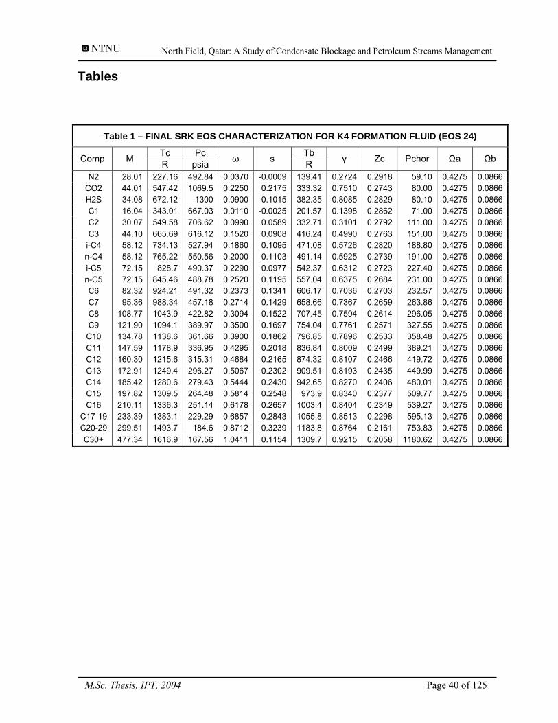
North Field, Qatar: A Study of Condensate Blockage and Petroleum Streams Management
Tables
Table 1 – FINAL SRK EOS CHARACTERIZATION FOR K4 FORMATION FLUID (EOS 24)
Tc Pc Tb Comp M R psia ω s R γ Zc Pchor Ωa Ωb
N2 28.01 227.16 492.84 0.0370 -0.0009 139.41 0.2724 0.2918 59.10 0.4275 0.0866 CO2 44.01 547.42 1069.5 0.2250 0.2175 333.32 0.7510 0.2743 80.00 0.4275 0.0866 H2S 34.08 672.12 1300 0.0900 0.1015 382.35 0.8085 0.2829 80.10 0.4275 0.0866 C1 16.04 343.01 667.03 0.0110 -0.0025 201.57 0.1398 0.2862 71.00 0.4275 0.0866 C2 30.07 549.58 706.62 0.0990 0.0589 332.71 0.3101 0.2792 111.00 0.4275 0.0866 C3 44.10 665.69 616.12 0.1520 0.0908 416.24 0.4990 0.2763 151.00 0.4275 0.0866
i-C4 58.12 734.13 527.94 0.1860 0.1095 471.08 0.5726 0.2820 188.80 0.4275 0.0866 n-C4 58.12 765.22 550.56 0.2000 0.1103 491.14 0.5925 0.2739 191.00 0.4275 0.0866 i-C5 72.15 828.7 490.37 0.2290 0.0977 542.37 0.6312 0.2723 227.40 0.4275 0.0866 n-C5 72.15 845.46 488.78 0.2520 0.1195 557.04 0.6375 0.2684 231.00 0.4275 0.0866 C6 82.32 924.21 491.32 0.2373 0.1341 606.17 0.7036 0.2703 232.57 0.4275 0.0866 C7 95.36 988.34 457.18 0.2714 0.1429 658.66 0.7367 0.2659 263.86 0.4275 0.0866 C8 108.77 1043.9 422.82 0.3094 0.1522 707.45 0.7594 0.2614 296.05 0.4275 0.0866 C9 121.90 1094.1 389.97 0.3500 0.1697 754.04 0.7761 0.2571 327.55 0.4275 0.0866
C10 134.78 1138.6 361.66 0.3900 0.1862 796.85 0.7896 0.2533 358.48 0.4275 0.0866 C11 147.59 1178.9 336.95 0.4295 0.2018 836.84 0.8009 0.2499 389.21 0.4275 0.0866 C12 160.30 1215.6 315.31 0.4684 0.2165 874.32 0.8107 0.2466 419.72 0.4275 0.0866 C13 172.91 1249.4 296.27 0.5067 0.2302 909.51 0.8193 0.2435 449.99 0.4275 0.0866 C14 185.42 1280.6 279.43 0.5444 0.2430 942.65 0.8270 0.2406 480.01 0.4275 0.0866 C15 197.82 1309.5 264.48 0.5814 0.2548 973.9 0.8340 0.2377 509.77 0.4275 0.0866 C16 210.11 1336.3 251.14 0.6178 0.2657 1003.4 0.8404 0.2349 539.27 0.4275 0.0866
C17-19 233.39 1383.1 229.29 0.6857 0.2843 1055.8 0.8513 0.2298 595.13 0.4275 0.0866 C20-29 299.51 1493.7 184.6 0.8712 0.3239 1183.8 0.8764 0.2161 753.83 0.4275 0.0866 C30+ 477.34 1616.9 167.56 1.0411 0.1154 1309.7 0.9215 0.2058 1180.62 0.4275 0.0866
M.Sc. Thesis, IPT, 2004 Page 40 of 125
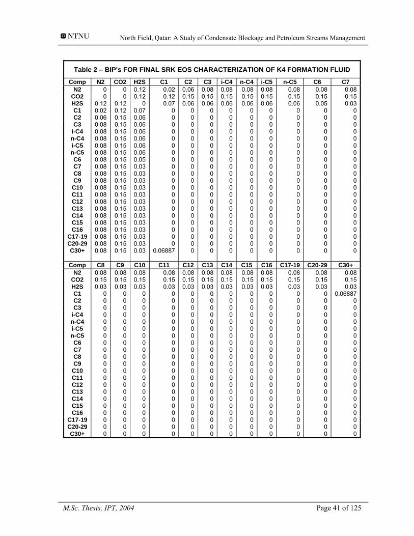
North Field, Qatar: A Study of Condensate Blockage and Petroleum Streams Management
Table 2 – BIP's FOR FINAL SRK EOS CHARACTERIZATION OF K4 FORMATION FLUID
Comp N2 CO2 H2S C1 C2 C3 i-C4 n-C4 i-C5 n-C5 C6 C7 N2 0 0 0.12 0.02 0.06 0.08 0.08 0.08 0.08 0.08 0.08 0.08
CO2 0 0 0.12 0.12 0.15 0.15 0.15 0.15 0.15 0.15 0.15 0.15H2S 0.12 0.12 0 0.07 0.06 0.06 0.06 0.06 0.06 0.06 0.05 0.03C1 0.02 0.12 0.07 0 0 0 0 0 0 0 0 0C2 0.06 0.15 0.06 0 0 0 0 0 0 0 0 0C3 0.08 0.15 0.06 0 0 0 0 0 0 0 0 0
i-C4 0.08 0.15 0.06 0 0 0 0 0 0 0 0 0n-C4 0.08 0.15 0.06 0 0 0 0 0 0 0 0 0i-C5 0.08 0.15 0.06 0 0 0 0 0 0 0 0 0n-C5 0.08 0.15 0.06 0 0 0 0 0 0 0 0 0C6 0.08 0.15 0.05 0 0 0 0 0 0 0 0 0C7 0.08 0.15 0.03 0 0 0 0 0 0 0 0 0C8 0.08 0.15 0.03 0 0 0 0 0 0 0 0 0C9 0.08 0.15 0.03 0 0 0 0 0 0 0 0 0
C10 0.08 0.15 0.03 0 0 0 0 0 0 0 0 0C11 0.08 0.15 0.03 0 0 0 0 0 0 0 0 0C12 0.08 0.15 0.03 0 0 0 0 0 0 0 0 0C13 0.08 0.15 0.03 0 0 0 0 0 0 0 0 0C14 0.08 0.15 0.03 0 0 0 0 0 0 0 0 0C15 0.08 0.15 0.03 0 0 0 0 0 0 0 0 0C16 0.08 0.15 0.03 0 0 0 0 0 0 0 0 0
C17-19 0.08 0.15 0.03 0 0 0 0 0 0 0 0 0C20-29 0.08 0.15 0.03 0 0 0 0 0 0 0 0 0C30+ 0.08 0.15 0.03 0.06887 0 0 0 0 0 0 0 0
Comp C8 C9 C10 C11 C12 C13 C14 C15 C16 C17-19 C20-29 C30+
N2 0.08 0.08 0.08 0.08 0.08 0.08 0.08 0.08 0.08 0.08 0.08 0.08CO2 0.15 0.15 0.15 0.15 0.15 0.15 0.15 0.15 0.15 0.15 0.15 0.15H2S 0.03 0.03 0.03 0.03 0.03 0.03 0.03 0.03 0.03 0.03 0.03 0.03C1 0 0 0 0 0 0 0 0 0 0 0 0.06887C2 0 0 0 0 0 0 0 0 0 0 0 0C3 0 0 0 0 0 0 0 0 0 0 0 0
i-C4 0 0 0 0 0 0 0 0 0 0 0 0n-C4 0 0 0 0 0 0 0 0 0 0 0 0i-C5 0 0 0 0 0 0 0 0 0 0 0 0n-C5 0 0 0 0 0 0 0 0 0 0 0 0C6 0 0 0 0 0 0 0 0 0 0 0 0C7 0 0 0 0 0 0 0 0 0 0 0 0C8 0 0 0 0 0 0 0 0 0 0 0 0C9 0 0 0 0 0 0 0 0 0 0 0 0
C10 0 0 0 0 0 0 0 0 0 0 0 0C11 0 0 0 0 0 0 0 0 0 0 0 0C12 0 0 0 0 0 0 0 0 0 0 0 0C13 0 0 0 0 0 0 0 0 0 0 0 0C14 0 0 0 0 0 0 0 0 0 0 0 0C15 0 0 0 0 0 0 0 0 0 0 0 0C16 0 0 0 0 0 0 0 0 0 0 0 0
C17-19 0 0 0 0 0 0 0 0 0 0 0 0C20-29 0 0 0 0 0 0 0 0 0 0 0 0C30+ 0 0 0 0 0 0 0 0 0 0 0 0
M.Sc. Thesis, IPT, 2004 Page 41 of 125
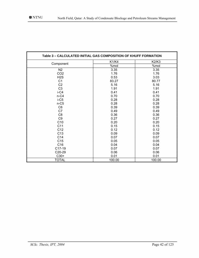
North Field, Qatar: A Study of Condensate Blockage and Petroleum Streams Management
Table 3 – CALCULATED INITIAL GAS COMPOSITION OF KHUFF FORMATION
K1/K4 K2/K3 Component %mol %mol N2 3.35 3.35
CO2 1.76 1.76 H2S 0.53 3.03 C1 83.27 80.77 C2 5.16 5.16 C3 1.91 1.91
i-C4 0.41 0.41 n-C4 0.70 0.70 i-C5 0.28 0.28 n-C5 0.28 0.28 C6 0.39 0.39 C7 0.49 0.49 C8 0.36 0.36 C9 0.27 0.27
C10 0.20 0.20 C11 0.15 0.15 C12 0.12 0.12 C13 0.09 0.09 C14 0.07 0.07 C15 0.05 0.05 C16 0.04 0.04
C17-19 0.07 0.07 C20-29 0.06 0.06 C30+ 0.01 0.01 TOTAL 100.00 100.00
M.Sc. Thesis, IPT, 2004 Page 42 of 125

North Field, Qatar: A Study of Condensate Blockage and Petroleum Streams Management
Table 4 – FULL FIELD RESERVOIR MODEL DESCRIPTION
GEOMETRY Surface Area 10 km x 10 km Gridding of Cartesian Model 20 x 20 x 17 Size of total reservoir, cuft 32808 x 32808 x 1721 DX = DY, ft 1640 (500 m) Depth to top of formation, ft 8050 ROCK AND FLUIDS PROPERTIES Porosity K1/K4 K2/K3
10 % 15 %
Permeability Layer kx=ky, md kz, md
K1 15 1.5 K2 45 4.5 K3 45 4.5 K4 15 1.5
Rock Compressibility, 1/psi 5.0E-06 Reservoir Temperature, F 220 Water compressibility, 1/psi 2.64E-06 Water FVF, RB/STB 1.0375 Water density, lbs/cuft 62.37 Water viscosity, cP 0.65 INITIAL CONDITION K4 Layer Initial Pressure, psig 5300 Reference Depth, ft 9600 Dew point pressure, psig 5120 K3 Layer Initial Pressure, psig 5180 Reference Depth, ft 8500 Dew point pressure, psig 4930 RELATIVE PERMEABILITY ANALYTICAL DATA Connate water saturation (Swi) 0.2 Residual oil saturation to water (Sorw) 0.2 Residual oil saturation to gas (Sorg) 0.2 Critical gas saturation (Sgc) 0.1 Relative permeability of water at Sw=1-Sorw, Sg=0 (krwro) 0.5 Relative permeability of gas at Sw=Swi, So=Sorg (krgro) 0.33 Relative permeability of oil at Sw=Swi, Sg=0 (krocw) 0.9 Exponent for krw curve (nw) 3 Exponent for krow curve (now) 3 Exponent for krg curve (ng) 3 Exponent for krog curve (nog) 3
M.Sc. Thesis, IPT, 2004 Page 43 of 125
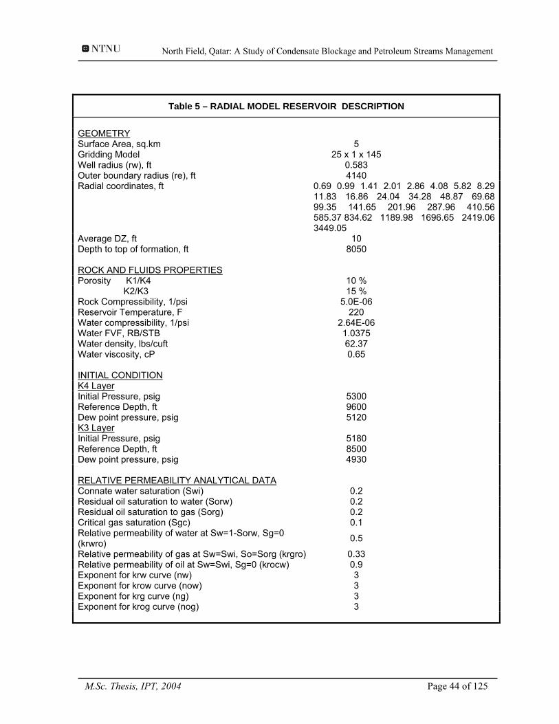
North Field, Qatar: A Study of Condensate Blockage and Petroleum Streams Management
Table 5 – RADIAL MODEL RESERVOIR DESCRIPTION
GEOMETRY Surface Area, sq.km 5 Gridding Model 25 x 1 x 145 Well radius (rw), ft 0.583 Outer boundary radius (re), ft 4140 Radial coordinates, ft 0.69 0.99 1.41 2.01 2.86 4.08 5.82 8.29
11.83 16.86 24.04 34.28 48.87 69.68 99.35 141.65 201.96 287.96 410.56 585.37 834.62 1189.98 1696.65 2419.06 3449.05
Average DZ, ft 10 Depth to top of formation, ft 8050 ROCK AND FLUIDS PROPERTIES Porosity K1/K4 10 % K2/K3 15 % Rock Compressibility, 1/psi 5.0E-06 Reservoir Temperature, F 220 Water compressibility, 1/psi 2.64E-06 Water FVF, RB/STB 1.0375 Water density, lbs/cuft 62.37 Water viscosity, cP 0.65 INITIAL CONDITION K4 Layer Initial Pressure, psig 5300 Reference Depth, ft 9600 Dew point pressure, psig 5120 K3 Layer Initial Pressure, psig 5180 Reference Depth, ft 8500 Dew point pressure, psig 4930 RELATIVE PERMEABILITY ANALYTICAL DATA Connate water saturation (Swi) 0.2 Residual oil saturation to water (Sorw) 0.2 Residual oil saturation to gas (Sorg) 0.2 Critical gas saturation (Sgc) 0.1 Relative permeability of water at Sw=1-Sorw, Sg=0 (krwro) 0.5
Relative permeability of gas at Sw=Swi, So=Sorg (krgro) 0.33 Relative permeability of oil at Sw=Swi, Sg=0 (krocw) 0.9 Exponent for krw curve (nw) 3 Exponent for krow curve (now) 3 Exponent for krg curve (ng) 3 Exponent for krog curve (nog) 3
M.Sc. Thesis, IPT, 2004 Page 44 of 125

North Field, Qatar: A Study of Condensate Blockage and Petroleum Streams Management
Table 6 – PERMEABILITY DISTRIBUTION FOR RADIAL MODEL
Permeability, md Geological Layer Average Minimum Maximum K1 16.7 0.1 299 K2 52.43 0.22 1295 K3 46.77 0.1 907 K4 17.7 0.1 429
Table 7 – PERMEABILITY DISTRIBUTION COMPARISON
Average Permeability, md Geological Layer Moderate Low Model Very Low Model K1 16.7 4.2 K2 52.43 13.11 K3 46.77 11.7 K4 17.7 4.43
Table 8 – RADIAL MODEL DESCRIPTION FOR CONDENSATE SKIN PREDICTION
Description K3 K4 Gridding Model 25 x 1 x 1 25 x 1 x 1 Well radius (rw), ft 0.583 0.583 Outer boundary radius (re), ft 4140 4140 Thickness, ft 170.07 160.71 Porosity 0.15 0.10 Permeability, md 46.77 17.70 Gas plateau rate,MMSCF/D 30 30
M.Sc. Thesis, IPT, 2004 Page 45 of 125

North Field, Qatar: A Study of Condensate Blockage and Petroleum Streams Management
Table 9 – GAS RATE COMPARISON
Time OGR Gas Rate, MMSCF/D Geological Layer
days STB/MMSCF Simulation Calculated %Diff K3 2735 22.54 30 30.62 2.1
K4 1825 22.72 17.12 17.43 1.8
Table 10 – CONDENSATE SKIN PREDICTION RESULT
Time OGR Gas Rate, MMSCF/D Skin factor Geological Layer days STB/MMSCF Simulation Rate
Dependent Dry Gas Simulation Rate
Dependent K3 2735 22.54 30 34.93 102.7 19.7 15.8
K4 1825 22.72 17.12 21.15 73.11 26.5 20
Table 11 – EFFECTIVE SKIN PREDICTION RESULT
Moderate Low Permeability Case Very Low Permeability Case Exponent K1 K2 K3 K4 K1 K2 K3 K4
3 17 13 15 12 16 18 18 16 1.5 3 3 3 3 3 3 3 3
M.Sc. Thesis, IPT, 2004 Page 46 of 125
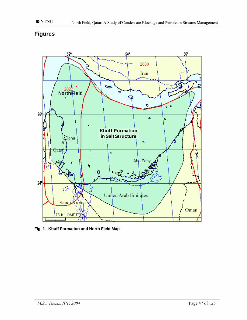
North Field, Qatar: A Study of Condensate Blockage and Petroleum Streams Management
Figures
Khuff Formationin Salt Structure
North Field
Fig. 1– Khuff Formation and North Field Map
M.Sc. Thesis, IPT, 2004 Page 47 of 125
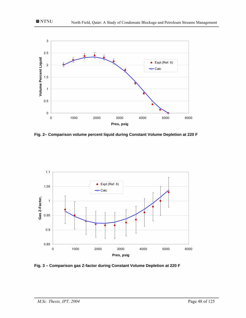
North Field, Qatar: A Study of Condensate Blockage and Petroleum Streams Management
0
0.5
1
1.5
2
2.5
3
0 1000 2000 3000 4000 5000 6000
Pres, psig
Volu
me
Perc
ent L
iqui
d
Expt (Ref. 6)
Calc
Fig. 2– Comparison volume percent liquid during Constant Volume Depletion at 220 F
0.85
0.9
0.95
1
1.05
1.1
0 1000 2000 3000 4000 5000 6000
Pres, psig
Gas
Z-F
acto
r,
Expt (Ref. 6)
Calc
Fig. 3 – Comparison gas Z-factor during Constant Volume Depletion at 220 F
M.Sc. Thesis, IPT, 2004 Page 48 of 125
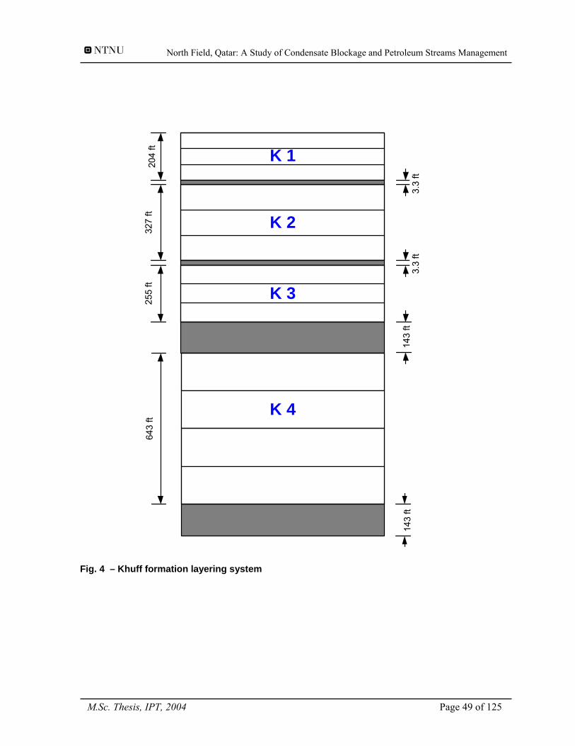
North Field, Qatar: A Study of Condensate Blockage and Petroleum Streams Management
K 2
204
ft K 1
K 4
K 3
327
ft25
5 ft
643
ft
3.3
ft3.
3 ft
143
ft14
3 ft
Fig. 4 – Khuff formation layering system
M.Sc. Thesis, IPT, 2004 Page 49 of 125

North Field, Qatar: A Study of Condensate Blockage and Petroleum Streams Management
Fig. 5 – North Field Production Well Position
M.Sc. Thesis, IPT, 2004 Page 50 of 125
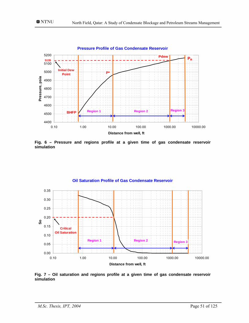
North Field, Qatar: A Study of Condensate Blockage and Petroleum Streams Management
Pressure Profile of Gas Condensate Reservoir
4400
4500
4600
4700
4800
4900
5000
5100
5200
0.10 1.00 10.00 100.00 1000.00 10000.00
Distance from well, ft
Pres
sure
, psi
a
5135
Initial Dew Point
Region 1 Region 2 Region 3BHFP
PR
P*
Pdew
Fig. 6 – Pressure and regions profile at a given time of gas condensate reservoir simulation
Oil Saturation Profile of Gas Condensate Reservoir
0.00
0.05
0.10
0.15
0.20
0.25
0.30
0.35
0.10 1.00 10.00 100.00 1000.00 10000.00
Distance from well, ft
So
Region 1 Region 2 Region 3
Critical Oil Saturation
Fig. 7 – Oil saturation and regions profile at a given time of gas condensate reservoir simulation
M.Sc. Thesis, IPT, 2004 Page 51 of 125
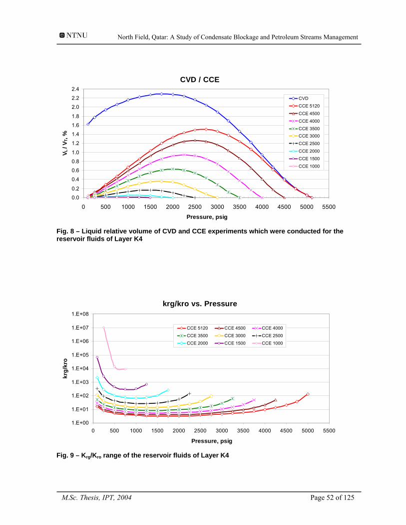
North Field, Qatar: A Study of Condensate Blockage and Petroleum Streams Management
CVD / CCE
0.0
0.2
0.4
0.6
0.8
1.0
1.2
1.4
1.6
1.8
2.0
2.2
2.4
0 500 1000 1500 2000 2500 3000 3500 4000 4500 5000 5500
Pressure, psig
V L /
V T, %
CVD
CCE 5120
CCE 4500
CCE 4000
CCE 3500CCE 3000
CCE 2500
CCE 2000
CCE 1500
CCE 1000
Fig. 8 – Liquid relative volume of CVD and CCE experiments which were conducted for the reservoir fluids of Layer K4
krg/kro vs. Pressure
1.E+00
1.E+01
1.E+02
1.E+03
1.E+04
1.E+05
1.E+06
1.E+07
1.E+08
0 500 1000 1500 2000 2500 3000 3500 4000 4500 5000 5500
Pressure, psig
krg/
kro
CCE 5120 CCE 4500 CCE 4000
CCE 3500 CCE 3000 CCE 2500
CCE 2000 CCE 1500 CCE 1000
Fig. 9 – Krg/Kro range of the reservoir fluids of Layer K4
M.Sc. Thesis, IPT, 2004 Page 52 of 125
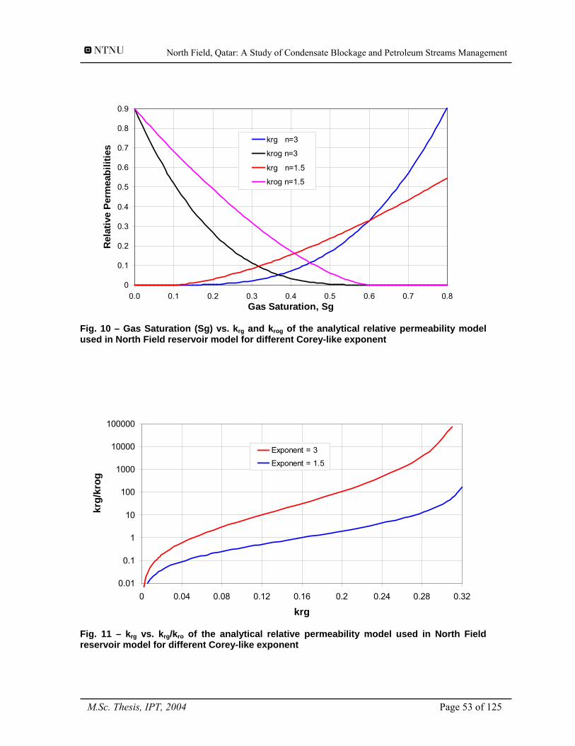
North Field, Qatar: A Study of Condensate Blockage and Petroleum Streams Management
0
0.1
0.2
0.3
0.4
0.5
0.6
0.7
0.8
0.9
0.0 0.1 0.2 0.3 0.4 0.5 0.6 0.7 0.8Gas Saturation, Sg
Rel
ativ
e Pe
rmea
bilit
ies
krg n=3
krog n=3
krg n=1.5
krog n=1.5
Fig. 10 – Gas Saturation (Sg) vs. krg and krog of the analytical relative permeability model used in North Field reservoir model for different Corey-like exponent
0.01
0.1
1
10
100
1000
10000
100000
0 0.04 0.08 0.12 0.16 0.2 0.24 0.28 0.32
krg
krg/
krog
Exponent = 3Exponent = 1.5
Fig. 11 – krg vs. krg/kro of the analytical relative permeability model used in North Field reservoir model for different Corey-like exponent
M.Sc. Thesis, IPT, 2004 Page 53 of 125
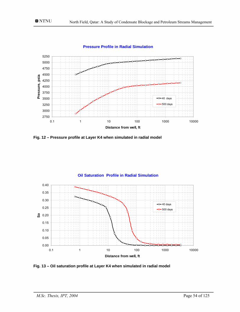
North Field, Qatar: A Study of Condensate Blockage and Petroleum Streams Management
Pressure Profile in Radial Simulation
2750
3000
3250
3500
3750
4000
4250
4500
4750
5000
5250
0.1 1 10 100 1000 10000
Distance from well, ft
Pres
sure
, psi
a
40 days
500 days
Fig. 12 – Pressure profile at Layer K4 when simulated in radial model
Oil Saturation Profile in Radial Simulation
0.00
0.05
0.10
0.15
0.20
0.25
0.30
0.35
0.40
0.1 1 10 100 1000 10000
Distance from well, ft
So
40 days
500 days
Fig. 13 – Oil saturation profile at Layer K4 when simulated in radial model
M.Sc. Thesis, IPT, 2004 Page 54 of 125
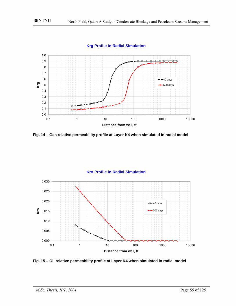
North Field, Qatar: A Study of Condensate Blockage and Petroleum Streams Management
Krg Profile in Radial Simulation
0.0
0.1
0.2
0.3
0.4
0.5
0.6
0.7
0.8
0.9
1.0
0.1 1 10 100 1000 10000
Distance from well, ft
Krg
40 days
500 days
Fig. 14 – Gas relative permeability profile at Layer K4 when simulated in radial model
Kro Profile in Radial Simulation
0.000
0.005
0.010
0.015
0.020
0.025
0.030
0.1 1 10 100 1000 10000
Distance from well, ft
Kro
40 days
500 days
Fig. 15 – Oil relative permeability profile at Layer K4 when simulated in radial model
M.Sc. Thesis, IPT, 2004 Page 55 of 125

North Field, Qatar: A Study of Condensate Blockage and Petroleum Streams Management
Absolute Permeability Distribution in K1k avg = 16.7 mD
0.01
0.1
1
10
100
1000
1 2 3 4 5 6 7 8 9 10 11 12 13 14 15 16 17 18 19 20
Layer No
k, m
D
Absolute Permeability
Fig. 16 – Absolute Permeability Distribution in K1
Absolute Permeability Distribution in K2k avg = 52.43 mD
0.1
1
10
100
1000
10000
22 24 26 28 30 32 34 36 38 40 42 44 46 48 50 52
Layer No
k, m
D
Absolute Permeability
Fig. 17 – Absolute Permeability Distribution in K2
M.Sc. Thesis, IPT, 2004 Page 56 of 125
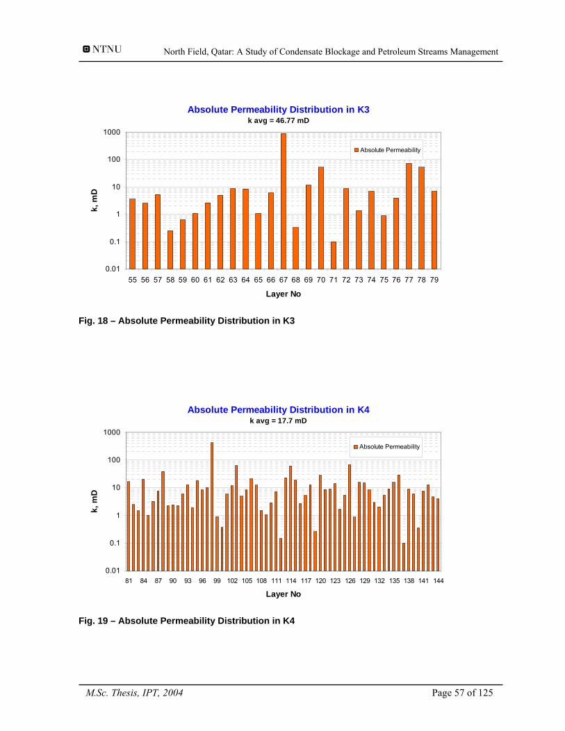
North Field, Qatar: A Study of Condensate Blockage and Petroleum Streams Management
Absolute Permeability Distribution in K3k avg = 46.77 mD
0.01
0.1
1
10
100
1000
55 56 57 58 59 60 61 62 63 64 65 66 67 68 69 70 71 72 73 74 75 76 77 78 79
Layer No
k, m
D
Absolute Permeability
Fig. 18 – Absolute Permeability Distribution in K3
Absolute Permeability Distribution in K4k avg = 17.7 mD
0.01
0.1
1
10
100
1000
81 84 87 90 93 96 99 102 105 108 111 114 117 120 123 126 129 132 135 138 141 144
Layer No
k, m
D
Absolute Permeability
Fig. 19 – Absolute Permeability Distribution in K4
M.Sc. Thesis, IPT, 2004 Page 57 of 125
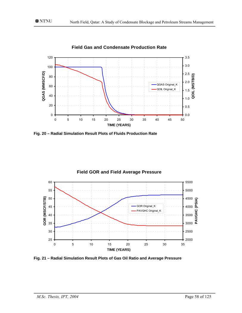
North Field, Qatar: A Study of Condensate Blockage and Petroleum Streams Management
Field Gas and Condensate Production Rate
0
20
40
60
80
100
120
0 5 10 15 20 25 30 35 40 45 50
TIME (YEARS)
QG
AS
(MM
SCF/
D)
0.0
0.5
1.0
1.5
2.0
2.5
3.0
3.5
QO
IL (M
STB
/D)
QGAS Original_K
QOIL Original_K
Fig. 20 – Radial Simulation Result Plots of Fluids Production Rate
Field GOR and Field Average Pressure
25
30
35
40
45
50
55
60
0 5 10 15 20 25 30 35
TIME (YEARS)
GO
R (M
SCF/
STB
)
2000
2500
3000
3500
4000
4500
5000
5500
PAVG
HC
(PSI
A)
GOR Original_K
PAVGHC Original_K
Fig. 21 – Radial Simulation Result Plots of Gas Oil Ratio and Average Pressure
M.Sc. Thesis, IPT, 2004 Page 58 of 125
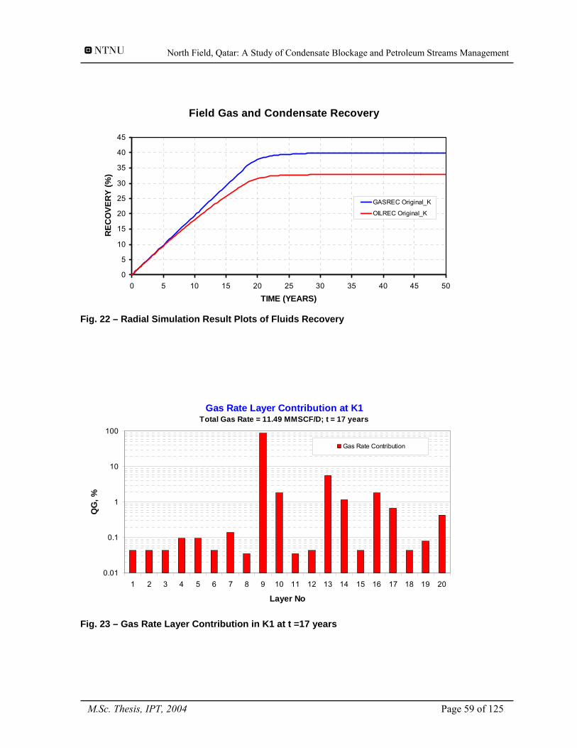
North Field, Qatar: A Study of Condensate Blockage and Petroleum Streams Management
Field Gas and Condensate Recovery
0
5
10
15
20
25
30
35
40
45
0 5 10 15 20 25 30 35 40 45 50
TIME (YEARS)
REC
OVE
RY
(%)
GASREC Original_K
OILREC Original_K
Fig. 22 – Radial Simulation Result Plots of Fluids Recovery
Gas Rate Layer Contribution at K1Total Gas Rate = 11.49 MMSCF/D; t = 17 years
0.01
0.1
1
10
100
1 2 3 4 5 6 7 8 9 10 11 12 13 14 15 16 17 18 19 20
Layer No
QG
, %
Gas Rate Contribution
Fig. 23 – Gas Rate Layer Contribution in K1 at t =17 years
M.Sc. Thesis, IPT, 2004 Page 59 of 125
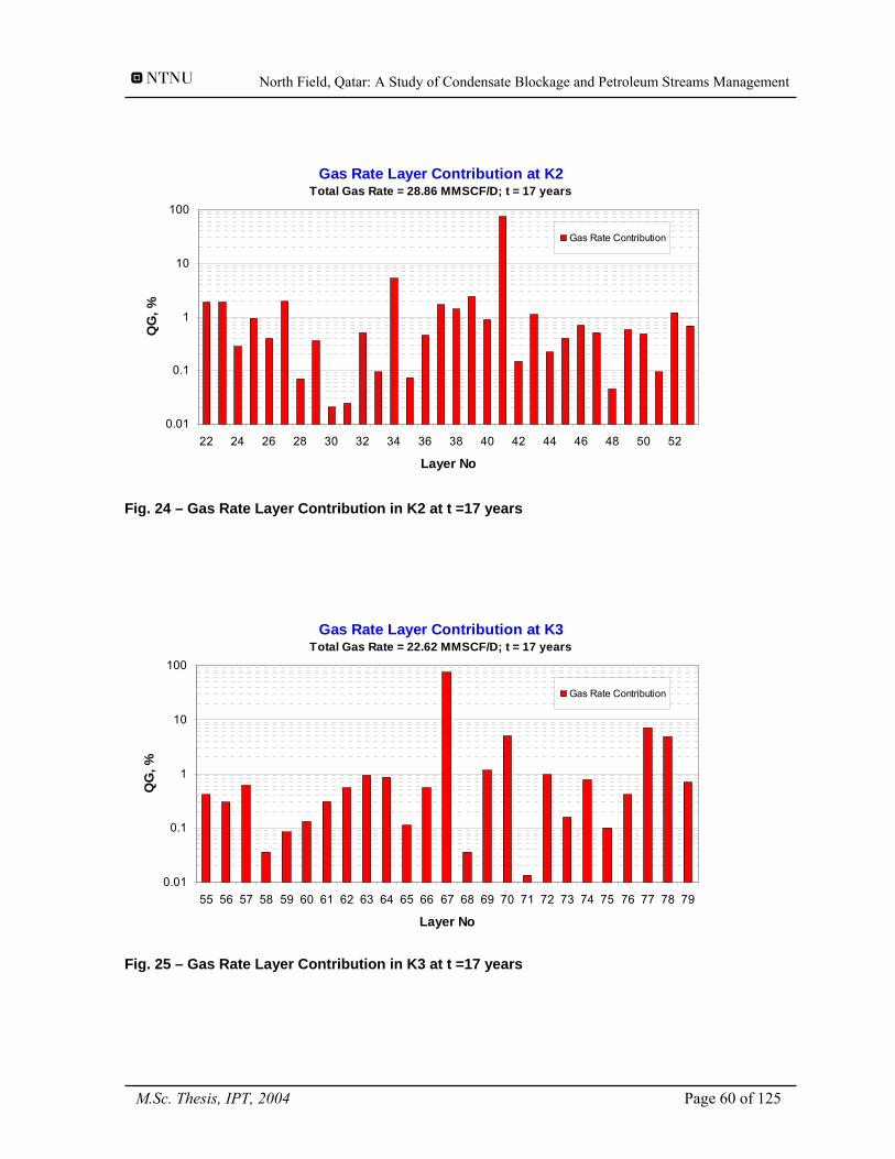
North Field, Qatar: A Study of Condensate Blockage and Petroleum Streams Management
Gas Rate Layer Contribution at K2Total Gas Rate = 28.86 MMSCF/D; t = 17 years
0.01
0.1
1
10
100
22 24 26 28 30 32 34 36 38 40 42 44 46 48 50 52
Layer No
QG
, %
Gas Rate Contribution
Fig. 24 – Gas Rate Layer Contribution in K2 at t =17 years
Gas Rate Layer Contribution at K3Total Gas Rate = 22.62 MMSCF/D; t = 17 years
0.01
0.1
1
10
100
55 56 57 58 59 60 61 62 63 64 65 66 67 68 69 70 71 72 73 74 75 76 77 78 79
Layer No
QG
, %
Gas Rate Contribution
Fig. 25 – Gas Rate Layer Contribution in K3 at t =17 years
M.Sc. Thesis, IPT, 2004 Page 60 of 125
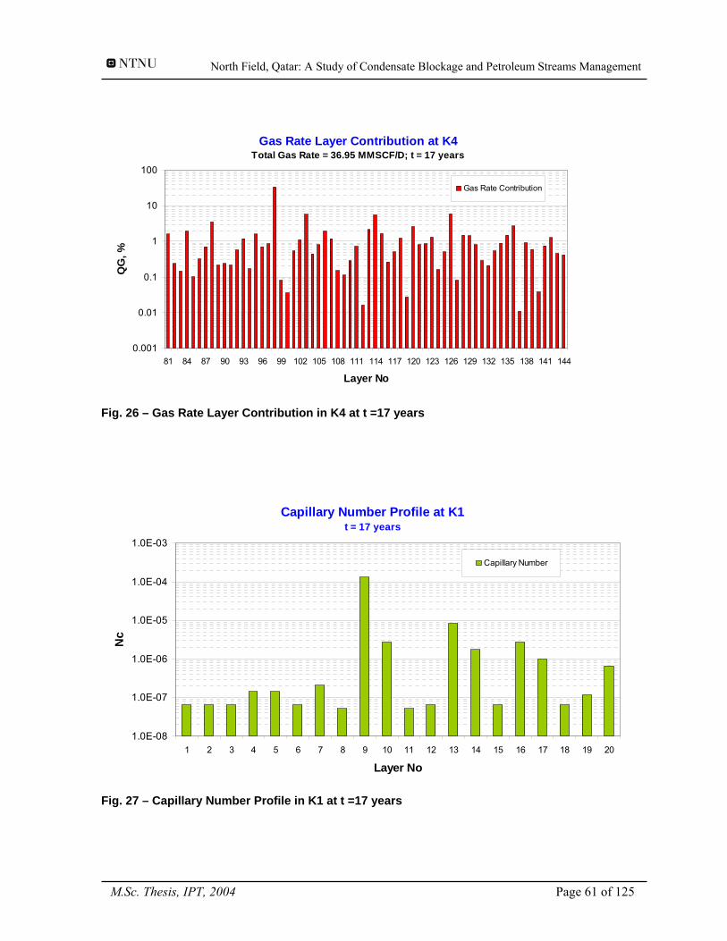
North Field, Qatar: A Study of Condensate Blockage and Petroleum Streams Management
Gas Rate Layer Contribution at K4Total Gas Rate = 36.95 MMSCF/D; t = 17 years
0.001
0.01
0.1
1
10
100
81 84 87 90 93 96 99 102 105 108 111 114 117 120 123 126 129 132 135 138 141 144
Layer No
QG
, %
Gas Rate Contribution
Fig. 26 – Gas Rate Layer Contribution in K4 at t =17 years
Capillary Number Profile at K1t = 17 years
1.0E-08
1.0E-07
1.0E-06
1.0E-05
1.0E-04
1.0E-03
1 2 3 4 5 6 7 8 9 10 11 12 13 14 15 16 17 18 19 20
Layer No
Nc
Capillary Number
Fig. 27 – Capillary Number Profile in K1 at t =17 years
M.Sc. Thesis, IPT, 2004 Page 61 of 125
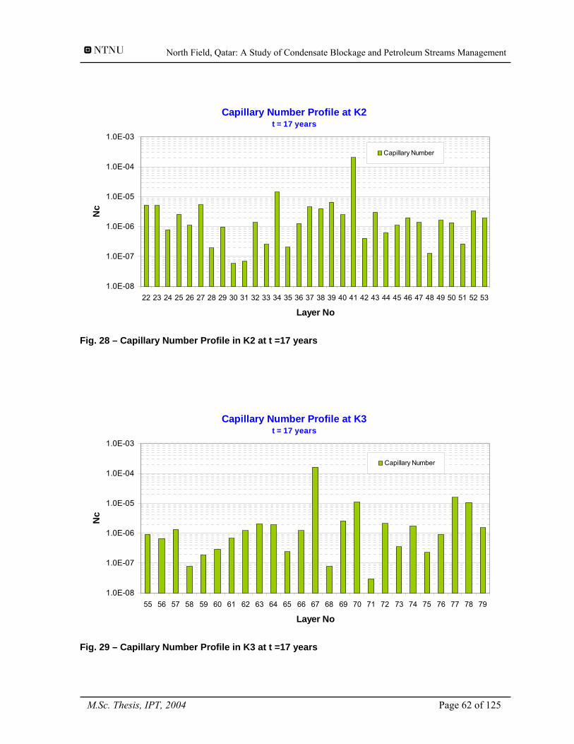
North Field, Qatar: A Study of Condensate Blockage and Petroleum Streams Management
Capillary Number Profile at K2t = 17 years
1.0E-08
1.0E-07
1.0E-06
1.0E-05
1.0E-04
1.0E-03
22 23 24 25 26 27 28 29 30 31 32 33 34 35 36 37 38 39 40 41 42 43 44 45 46 47 48 49 50 51 52 53
Layer No
Nc
Capillary Number
Fig. 28 – Capillary Number Profile in K2 at t =17 years
Capillary Number Profile at K3t = 17 years
1.0E-08
1.0E-07
1.0E-06
1.0E-05
1.0E-04
1.0E-03
55 56 57 58 59 60 61 62 63 64 65 66 67 68 69 70 71 72 73 74 75 76 77 78 79
Layer No
Nc
Capillary Number
Fig. 29 – Capillary Number Profile in K3 at t =17 years
M.Sc. Thesis, IPT, 2004 Page 62 of 125
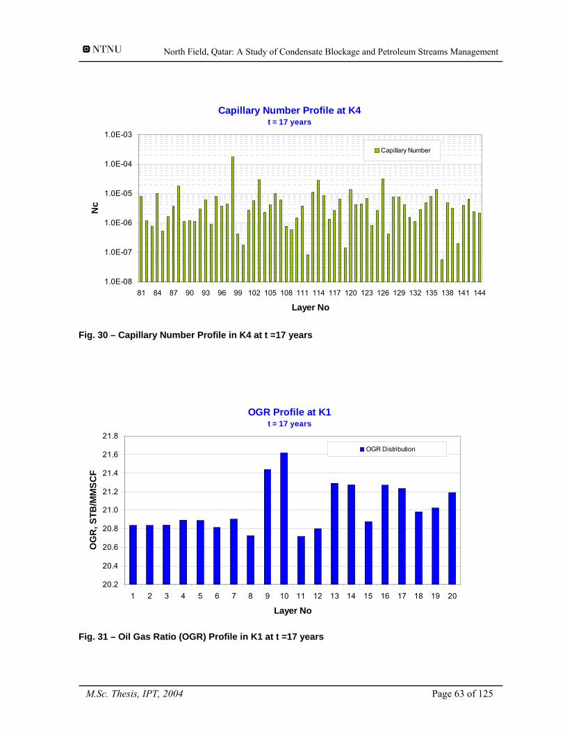
North Field, Qatar: A Study of Condensate Blockage and Petroleum Streams Management
Capillary Number Profile at K4t = 17 years
1.0E-08
1.0E-07
1.0E-06
1.0E-05
1.0E-04
1.0E-03
81 84 87 90 93 96 99 102 105 108 111 114 117 120 123 126 129 132 135 138 141 144
Layer No
Nc
Capillary Number
Fig. 30 – Capillary Number Profile in K4 at t =17 years
OGR Profile at K1t = 17 years
20.2
20.4
20.6
20.8
21.0
21.2
21.4
21.6
21.8
1 2 3 4 5 6 7 8 9 10 11 12 13 14 15 16 17 18 19 20
Layer No
OG
R, S
TB/M
MSC
F
OGR Distribution
Fig. 31 – Oil Gas Ratio (OGR) Profile in K1 at t =17 years
M.Sc. Thesis, IPT, 2004 Page 63 of 125
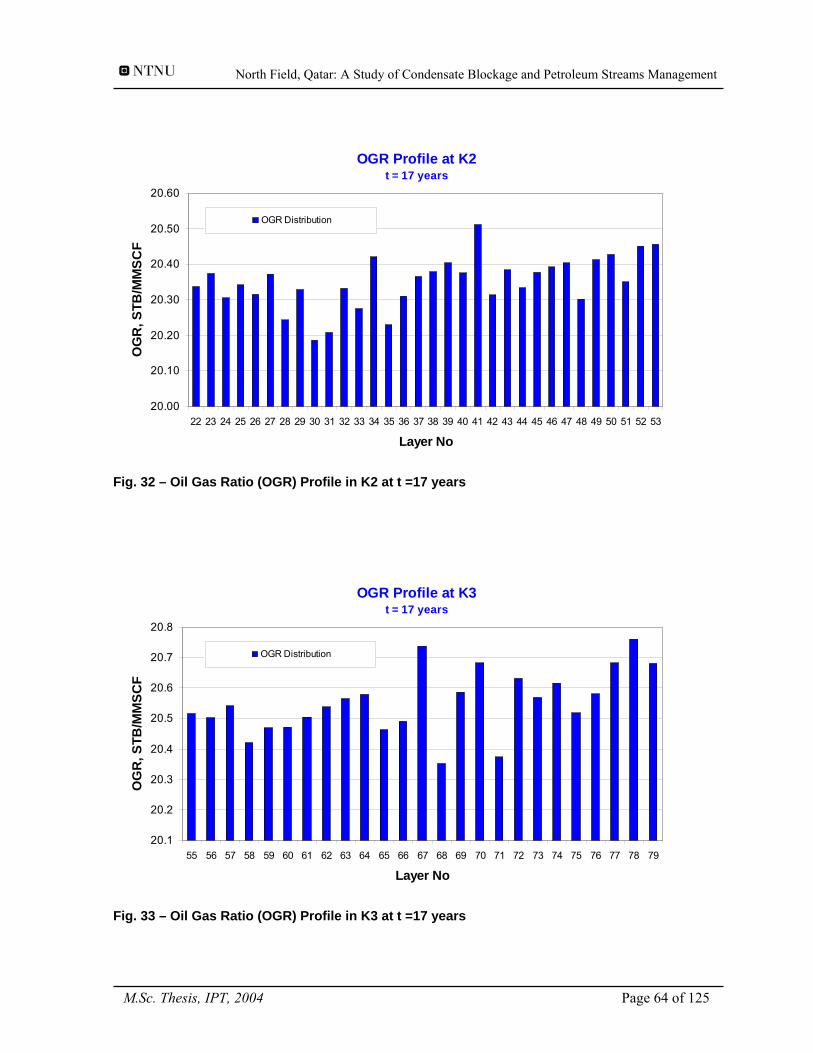
North Field, Qatar: A Study of Condensate Blockage and Petroleum Streams Management
OGR Profile at K2t = 17 years
20.00
20.10
20.20
20.30
20.40
20.50
20.60
22 23 24 25 26 27 28 29 30 31 32 33 34 35 36 37 38 39 40 41 42 43 44 45 46 47 48 49 50 51 52 53
Layer No
OG
R, S
TB/M
MSC
F
OGR Distribution
Fig. 32 – Oil Gas Ratio (OGR) Profile in K2 at t =17 years
OGR Profile at K3t = 17 years
20.1
20.2
20.3
20.4
20.5
20.6
20.7
20.8
55 56 57 58 59 60 61 62 63 64 65 66 67 68 69 70 71 72 73 74 75 76 77 78 79
Layer No
OG
R, S
TB/M
MSC
F
OGR Distribution
Fig. 33 – Oil Gas Ratio (OGR) Profile in K3 at t =17 years
M.Sc. Thesis, IPT, 2004 Page 64 of 125
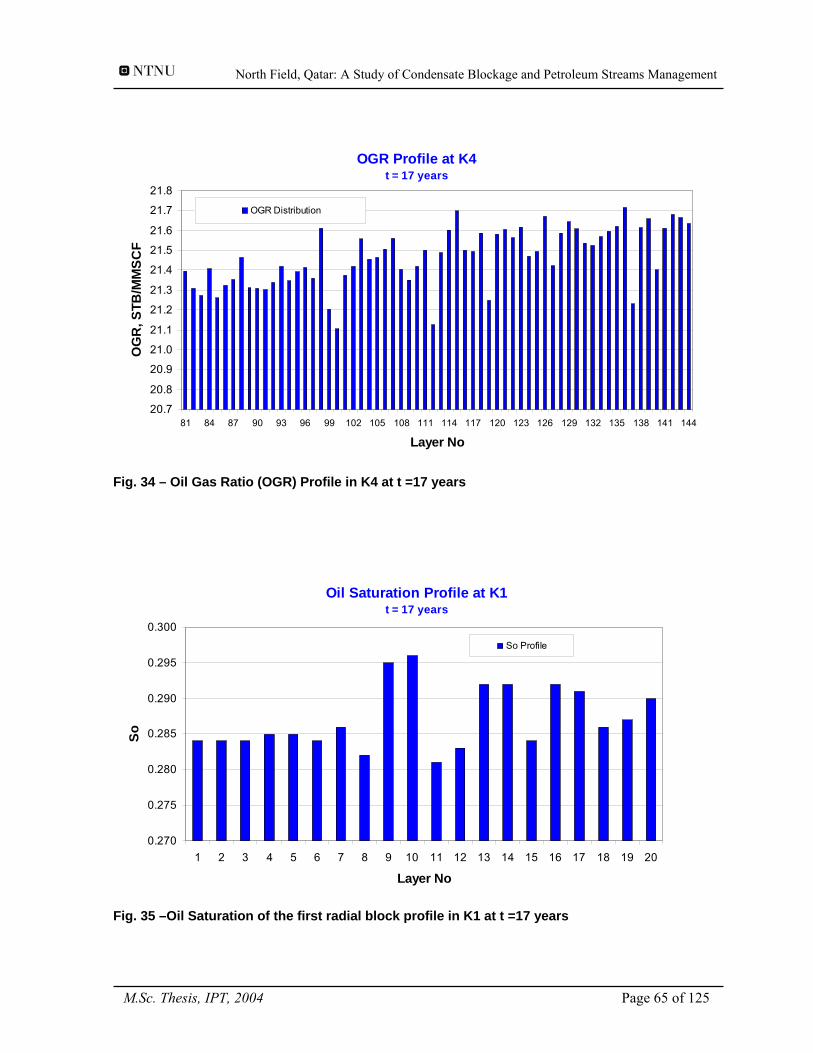
North Field, Qatar: A Study of Condensate Blockage and Petroleum Streams Management
OGR Profile at K4t = 17 years
20.7
20.8
20.9
21.0
21.1
21.2
21.3
21.4
21.5
21.6
21.7
21.8
81 84 87 90 93 96 99 102 105 108 111 114 117 120 123 126 129 132 135 138 141 144
Layer No
OG
R, S
TB/M
MSC
F
OGR Distribution
Fig. 34 – Oil Gas Ratio (OGR) Profile in K4 at t =17 years
Oil Saturation Profile at K1t = 17 years
0.270
0.275
0.280
0.285
0.290
0.295
0.300
1 2 3 4 5 6 7 8 9 10 11 12 13 14 15 16 17 18 19 20
Layer No
So
So Profile
Fig. 35 –Oil Saturation of the first radial block profile in K1 at t =17 years
M.Sc. Thesis, IPT, 2004 Page 65 of 125
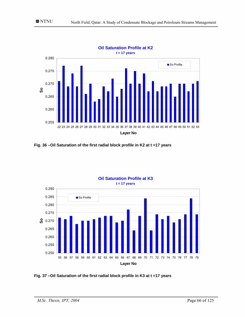
North Field, Qatar: A Study of Condensate Blockage and Petroleum Streams Management
Oil Saturation Profile at K2t = 17 years
0.255
0.260
0.265
0.270
0.275
0.280
22 23 24 25 26 27 28 29 30 31 32 33 34 35 36 37 38 39 40 41 42 43 44 45 46 47 48 49 50 51 52 53
Layer No
So
So Profile
Fig. 36 –Oil Saturation of the first radial block profile in K2 at t =17 years
Oil Saturation Profile at K3t = 17 years
0.250
0.255
0.260
0.265
0.270
0.275
0.280
0.285
0.290
55 56 57 58 59 60 61 62 63 64 65 66 67 68 69 70 71 72 73 74 75 76 77 78 79
Layer No
So
So Profile
Fig. 37 –Oil Saturation of the first radial block profile in K3 at t =17 years
M.Sc. Thesis, IPT, 2004 Page 66 of 125
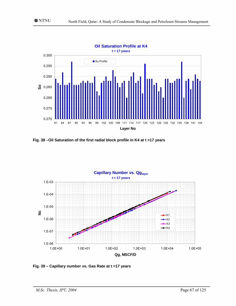
North Field, Qatar: A Study of Condensate Blockage and Petroleum Streams Management
Oil Saturation Profile at K4t = 17 years
0.270
0.275
0.280
0.285
0.290
0.295
0.300
81 84 87 90 93 96 99 102 105 108 111 114 117 120 123 126 129 132 135 138 141 144
Layer No
So
So Profile
Fig. 38 –Oil Saturation of the first radial block profile in K4 at t =17 years
Capillary Number vs. Qglayert = 17 years
1.E-08
1.E-07
1.E-06
1.E-05
1.E-04
1.E-03
1.0E+00 1.0E+01 1.0E+02 1.0E+03 1.0E+04 1.0E+05
Qg, MSCF/D
Nc
K1K2K3K4
Fig. 39 – Capillary number vs. Gas Rate at t =17 years
M.Sc. Thesis, IPT, 2004 Page 67 of 125
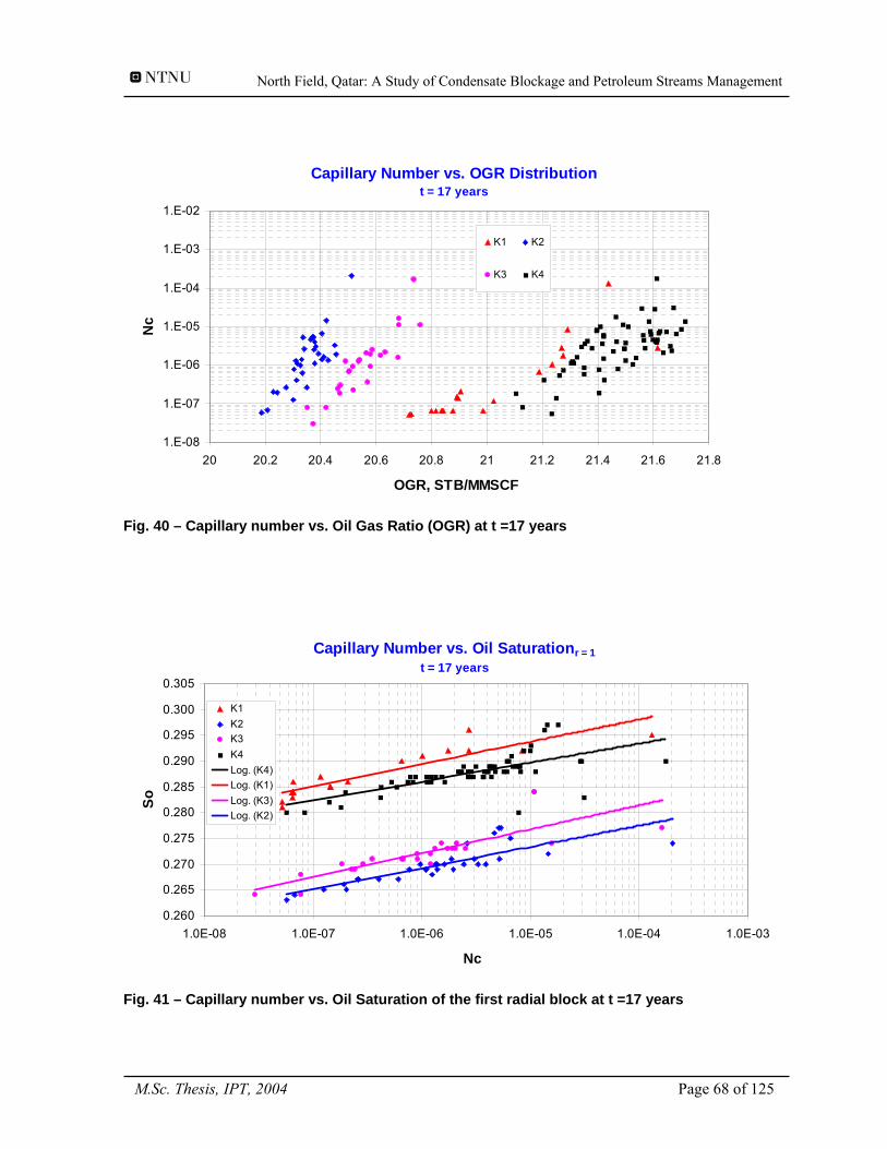
North Field, Qatar: A Study of Condensate Blockage and Petroleum Streams Management
Capillary Number vs. OGR Distributiont = 17 years
1.E-08
1.E-07
1.E-06
1.E-05
1.E-04
1.E-03
1.E-02
20 20.2 20.4 20.6 20.8 21 21.2 21.4 21.6 21.8
OGR, STB/MMSCF
Nc
K1 K2
K3 K4
Fig. 40 – Capillary number vs. Oil Gas Ratio (OGR) at t =17 years
Capillary Number vs. Oil Saturationr = 1t = 17 years
0.260
0.265
0.270
0.275
0.280
0.285
0.290
0.295
0.300
0.305
1.0E-08 1.0E-07 1.0E-06 1.0E-05 1.0E-04 1.0E-03
Nc
So
K1K2K3K4Log. (K4)Log. (K1)Log. (K3)Log. (K2)
Fig. 41 – Capillary number vs. Oil Saturation of the first radial block at t =17 years
M.Sc. Thesis, IPT, 2004 Page 68 of 125
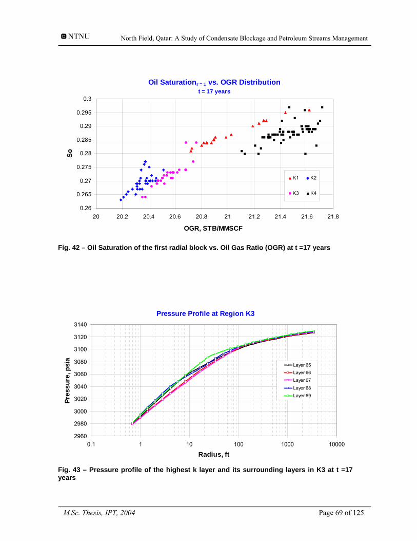
North Field, Qatar: A Study of Condensate Blockage and Petroleum Streams Management
Oil Saturationr = 1 vs. OGR Distributiont = 17 years
0.26
0.265
0.27
0.275
0.28
0.285
0.29
0.295
0.3
20 20.2 20.4 20.6 20.8 21 21.2 21.4 21.6 21.8
OGR, STB/MMSCF
So
K1 K2
K3 K4
Fig. 42 – Oil Saturation of the first radial block vs. Oil Gas Ratio (OGR) at t =17 years
Pressure Profile at Region K3
2960
2980
3000
3020
3040
3060
3080
3100
3120
3140
0.1 1 10 100 1000 10000
Radius, ft
Pres
sure
, psi
a
Layer 65Layer 66Layer 67
Layer 68Layer 69
Fig. 43 – Pressure profile of the highest k layer and its surrounding layers in K3 at t =17 years
M.Sc. Thesis, IPT, 2004 Page 69 of 125
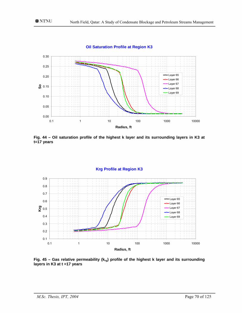
North Field, Qatar: A Study of Condensate Blockage and Petroleum Streams Management
Oil Saturation Profile at Region K3
0.00
0.05
0.10
0.15
0.20
0.25
0.30
0.1 1 10 100 1000 10000
Radius, ft
So
Layer 65Layer 66Layer 67
Layer 68Layer 69
Fig. 44 – Oil saturation profile of the highest k layer and its surrounding layers in K3 at t=17 years
Krg Profile at Region K3
0.1
0.2
0.3
0.4
0.5
0.6
0.7
0.8
0.9
0.1 1 10 100 1000 10000
Radius, ft
Krg
Layer 65Layer 66Layer 67
Layer 68Layer 69
Fig. 45 – Gas relative permeability (krg) profile of the highest k layer and its surrounding layers in K3 at t =17 years
M.Sc. Thesis, IPT, 2004 Page 70 of 125
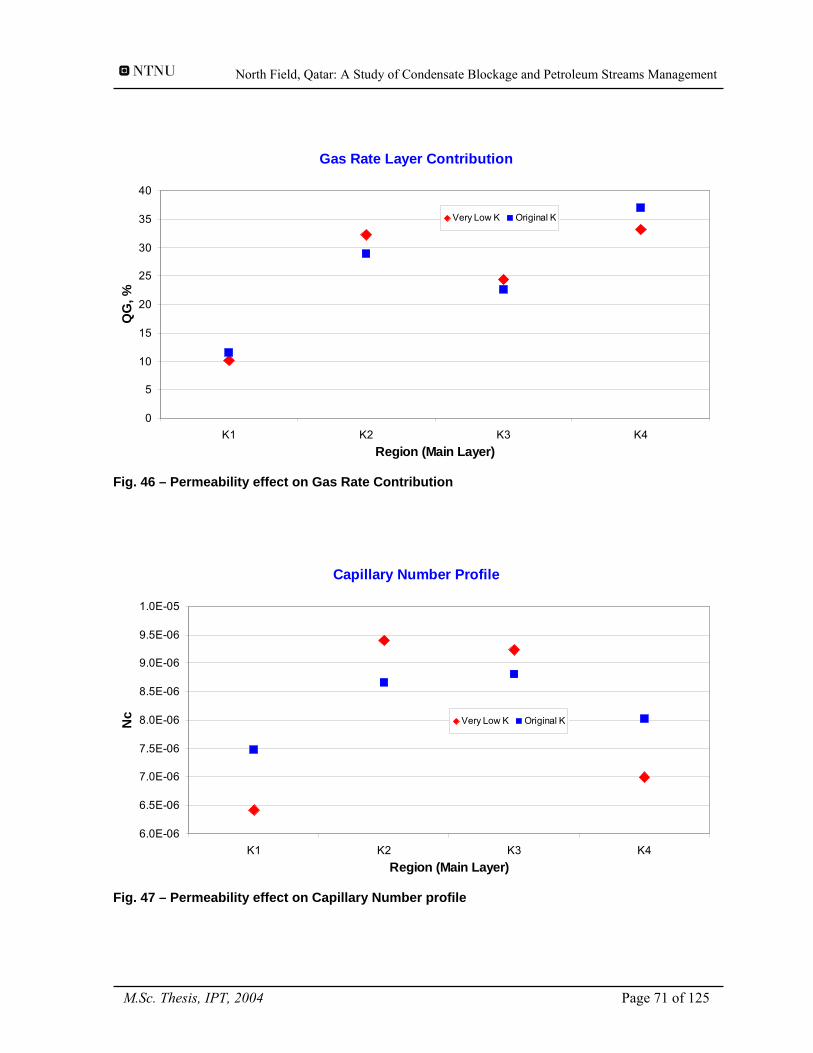
North Field, Qatar: A Study of Condensate Blockage and Petroleum Streams Management
Gas Rate Layer Contribution
0
5
10
15
20
25
30
35
40
K1 K2 K3 K4Region (Main Layer)
QG
, %
Very Low K Original K
Fig. 46 – Permeability effect on Gas Rate Contribution
Capillary Number Profile
6.0E-06
6.5E-06
7.0E-06
7.5E-06
8.0E-06
8.5E-06
9.0E-06
9.5E-06
1.0E-05
K1 K2 K3 K4Region (Main Layer)
Nc Very Low K Original K
Fig. 47 – Permeability effect on Capillary Number profile
M.Sc. Thesis, IPT, 2004 Page 71 of 125
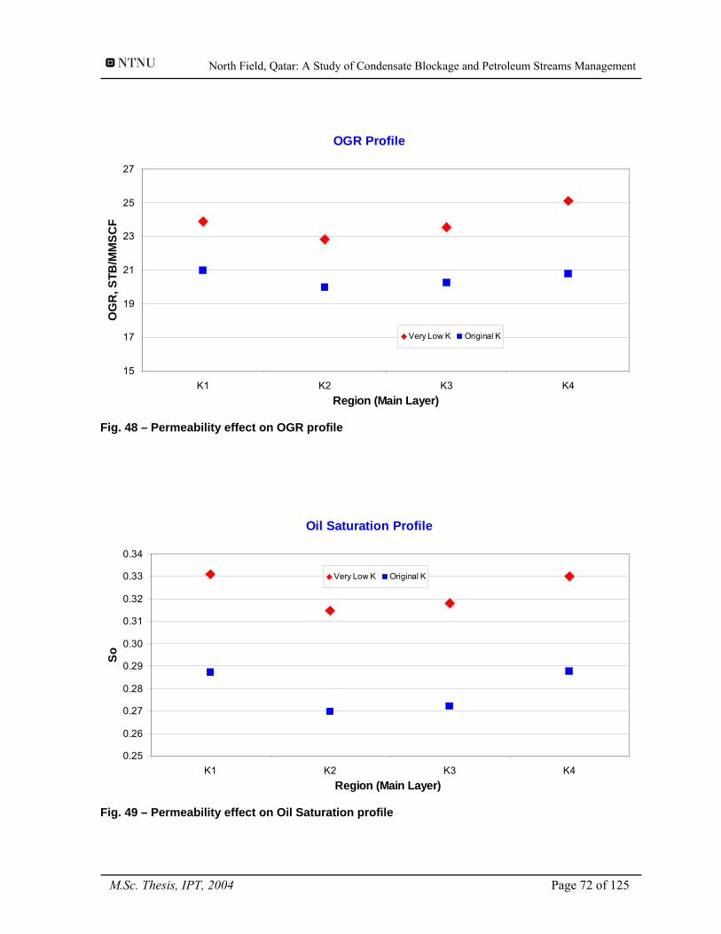
North Field, Qatar: A Study of Condensate Blockage and Petroleum Streams Management
OGR Profile
15
17
19
21
23
25
27
K1 K2 K3 K4Region (Main Layer)
OG
R, S
TB/M
MSC
F
Very Low K Original K
Fig. 48 – Permeability effect on OGR profile
Oil Saturation Profile
0.25
0.26
0.27
0.28
0.29
0.30
0.31
0.32
0.33
0.34
K1 K2 K3 K4Region (Main Layer)
So
Very Low K Original K
Fig. 49 – Permeability effect on Oil Saturation profile
M.Sc. Thesis, IPT, 2004 Page 72 of 125
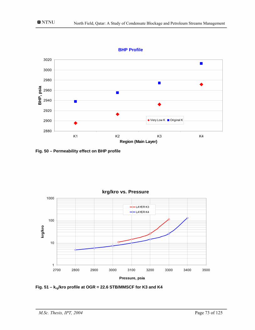
North Field, Qatar: A Study of Condensate Blockage and Petroleum Streams Management
BHP Profile
2880
2900
2920
2940
2960
2980
3000
3020
K1 K2 K3 K4Region (Main Layer)
BH
P, p
sia
Very Low K Original K
Fig. 50 – Permeability effect on BHP profile
krg/kro vs. Pressure
1
10
100
1000
2700 2800 2900 3000 3100 3200 3300 3400 3500
Pressure, psia
krg/
kro
LAYER K3
LAYER K4
Fig. 51 – krg/kro profile at OGR = 22.6 STB/MMSCF for K3 and K4
M.Sc. Thesis, IPT, 2004 Page 73 of 125
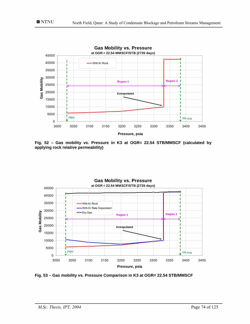
North Field, Qatar: A Study of Condensate Blockage and Petroleum Streams Management
Gas Mobility vs. Pressureat OGR = 22.54 MMSCF/STB (2735 days)
0
5000
10000
15000
20000
25000
30000
35000
40000
45000
3000 3050 3100 3150 3200 3250 3300 3350 3400 3450
Pressure, psia
Gas
Mob
ility
With Kr Rock
Extrapolated
PBH PR avg
Region 1 Region 2
Fig. 52 – Gas mobility vs. Pressure in K3 at OGR= 22.54 STB/MMSCF (calculated by applying rock relative permeability)
Gas Mobility vs. Pressureat OGR = 22.54 MMSCF/STB (2735 days)
0
5000
10000
15000
20000
25000
30000
35000
40000
45000
3000 3050 3100 3150 3200 3250 3300 3350 3400 3450
Pressure, psia
Gas
Mob
ility
With Kr RockWith Kr Rate DependentDry Gas
Extrapolated
PBH PR avg
Region 1 Region 2
Fig. 53 – Gas mobility vs. Pressure Comparison in K3 at OGR= 22.54 STB/MMSCF
M.Sc. Thesis, IPT, 2004 Page 74 of 125
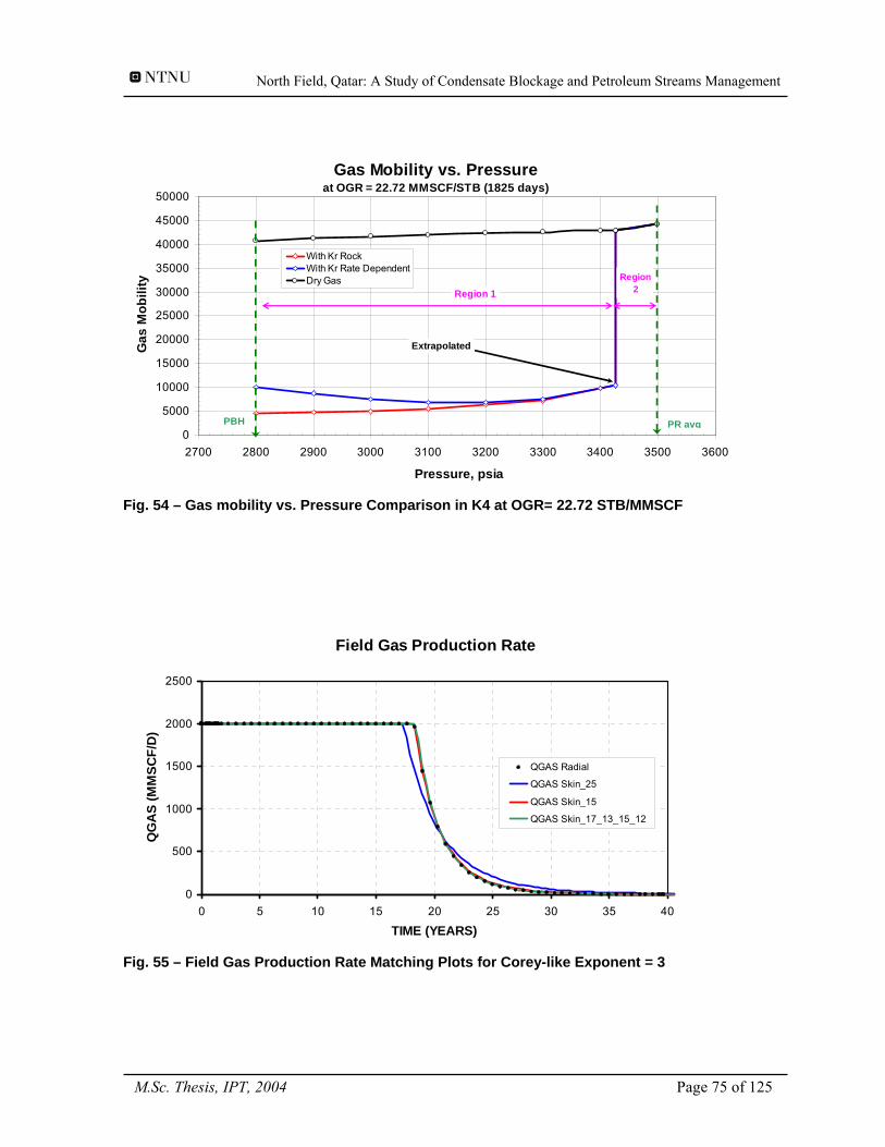
North Field, Qatar: A Study of Condensate Blockage and Petroleum Streams Management
Gas Mobility vs. Pressureat OGR = 22.72 MMSCF/STB (1825 days)
0
5000
10000
15000
20000
25000
30000
35000
40000
45000
50000
2700 2800 2900 3000 3100 3200 3300 3400 3500 3600
Pressure, psia
Gas
Mob
ility
With Kr RockWith Kr Rate DependentDry Gas
Extrapolated
PBH PR avg
Region 1
Region 2
Fig. 54 – Gas mobility vs. Pressure Comparison in K4 at OGR= 22.72 STB/MMSCF
Field Gas Production Rate
0
500
1000
1500
2000
2500
0 5 10 15 20 25 30 35 40
TIME (YEARS)
QG
AS
(MM
SCF/
D)
QGAS Radial
QGAS Skin_25
QGAS Skin_15
QGAS Skin_17_13_15_12
Fig. 55 – Field Gas Production Rate Matching Plots for Corey-like Exponent = 3
M.Sc. Thesis, IPT, 2004 Page 75 of 125
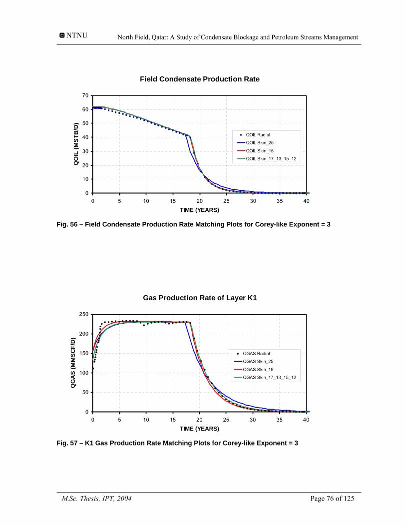
North Field, Qatar: A Study of Condensate Blockage and Petroleum Streams Management
Field Condensate Production Rate
0
10
20
30
40
50
60
70
0 5 10 15 20 25 30 35 40
TIME (YEARS)
QO
IL (M
STB
/D)
QOIL Radial
QOIL Skin_25
QOIL Skin_15
QOIL Skin_17_13_15_12
Fig. 56 – Field Condensate Production Rate Matching Plots for Corey-like Exponent = 3
Gas Production Rate of Layer K1
0
50
100
150
200
250
0 5 10 15 20 25 30 35 40
TIME (YEARS)
QG
AS
(MM
SCF/
D)
QGAS Radial
QGAS Skin_25
QGAS Skin_15
QGAS Skin_17_13_15_12
Fig. 57 – K1 Gas Production Rate Matching Plots for Corey-like Exponent = 3
M.Sc. Thesis, IPT, 2004 Page 76 of 125
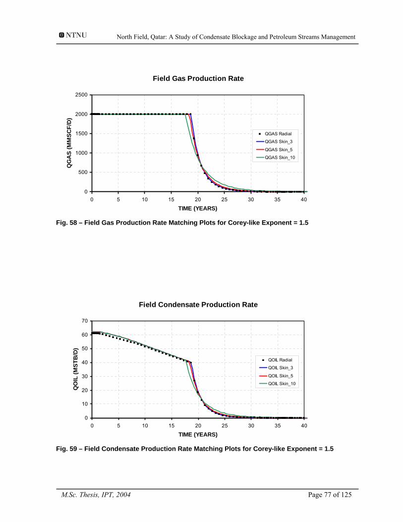
North Field, Qatar: A Study of Condensate Blockage and Petroleum Streams Management
Field Gas Production Rate
0
500
1000
1500
2000
2500
0 5 10 15 20 25 30 35 40
TIME (YEARS)
QG
AS
(MM
SCF/
D)
QGAS Radial
QGAS Skin_3
QGAS Skin_5
QGAS Skin_10
Fig. 58 – Field Gas Production Rate Matching Plots for Corey-like Exponent = 1.5
Field Condensate Production Rate
0
10
20
30
40
50
60
70
0 5 10 15 20 25 30 35 40
TIME (YEARS)
QO
IL (M
STB
/D)
QOIL Radial
QOIL Skin_3
QOIL Skin_5
QOIL Skin_10
Fig. 59 – Field Condensate Production Rate Matching Plots for Corey-like Exponent = 1.5
M.Sc. Thesis, IPT, 2004 Page 77 of 125
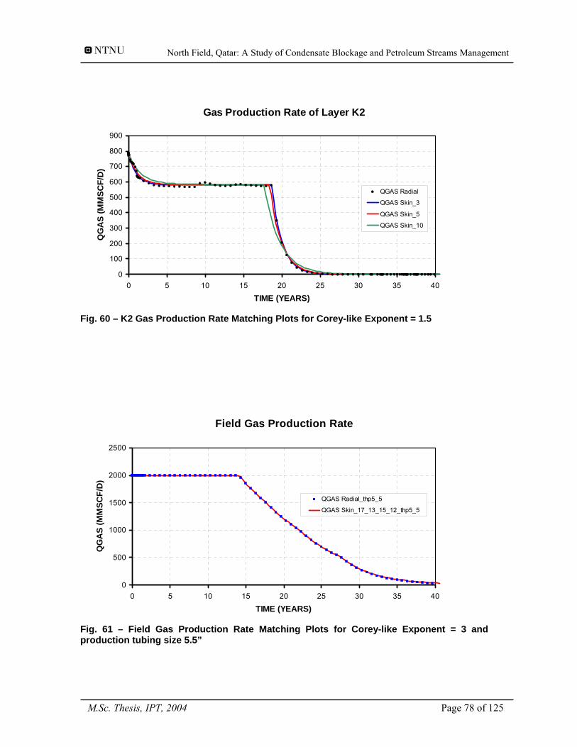
North Field, Qatar: A Study of Condensate Blockage and Petroleum Streams Management
Gas Production Rate of Layer K2
0
100
200
300
400
500
600
700
800
900
0 5 10 15 20 25 30 35 40
TIME (YEARS)
QG
AS
(MM
SCF/
D)
QGAS Radial
QGAS Skin_3
QGAS Skin_5
QGAS Skin_10
Fig. 60 – K2 Gas Production Rate Matching Plots for Corey-like Exponent = 1.5
Field Gas Production Rate
0
500
1000
1500
2000
2500
0 5 10 15 20 25 30 35 40
TIME (YEARS)
QG
AS
(MM
SCF/
D)
QGAS Radial_thp5_5
QGAS Skin_17_13_15_12_thp5_5
Fig. 61 – Field Gas Production Rate Matching Plots for Corey-like Exponent = 3 and production tubing size 5.5”
M.Sc. Thesis, IPT, 2004 Page 78 of 125
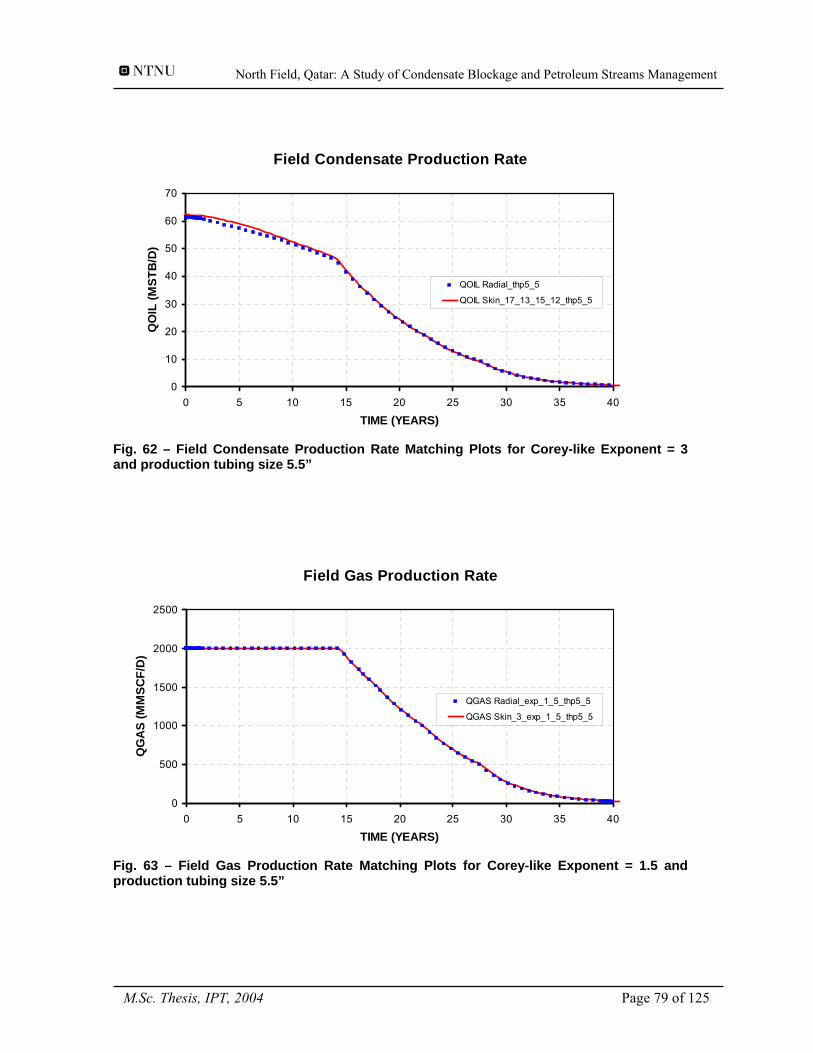
North Field, Qatar: A Study of Condensate Blockage and Petroleum Streams Management
Field Condensate Production Rate
0
10
20
30
40
50
60
70
0 5 10 15 20 25 30 35 40
TIME (YEARS)
QO
IL (M
STB
/D)
QOIL Radial_thp5_5
QOIL Skin_17_13_15_12_thp5_5
Fig. 62 – Field Condensate Production Rate Matching Plots for Corey-like Exponent = 3 and production tubing size 5.5”
Field Gas Production Rate
0
500
1000
1500
2000
2500
0 5 10 15 20 25 30 35 40
TIME (YEARS)
QG
AS
(MM
SCF/
D)
QGAS Radial_exp_1_5_thp5_5
QGAS Skin_3_exp_1_5_thp5_5
Fig. 63 – Field Gas Production Rate Matching Plots for Corey-like Exponent = 1.5 and production tubing size 5.5”
M.Sc. Thesis, IPT, 2004 Page 79 of 125
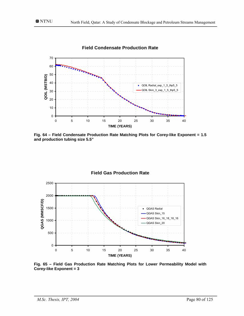
North Field, Qatar: A Study of Condensate Blockage and Petroleum Streams Management
Field Condensate Production Rate
0
10
20
30
40
50
60
70
0 5 10 15 20 25 30 35 40
TIME (YEARS)
QO
IL (M
STB
/D)
QOIL Radial_exp_1_5_thp5_5
QOIL Skin_3_exp_1_5_thp5_5
Fig. 64 – Field Condensate Production Rate Matching Plots for Corey-like Exponent = 1.5 and production tubing size 5.5”
Field Gas Production Rate
0
500
1000
1500
2000
2500
0 5 10 15 20 25 30 35 40
TIME (YEARS)
QG
AS
(MM
SCF/
D)
QGAS Radial
QGAS Skin_15
QGAS Skin_16_18_18_16
QGAS Skin_20
Fig. 65 – Field Gas Production Rate Matching Plots for Lower Permeability Model with Corey-like Exponent = 3
M.Sc. Thesis, IPT, 2004 Page 80 of 125
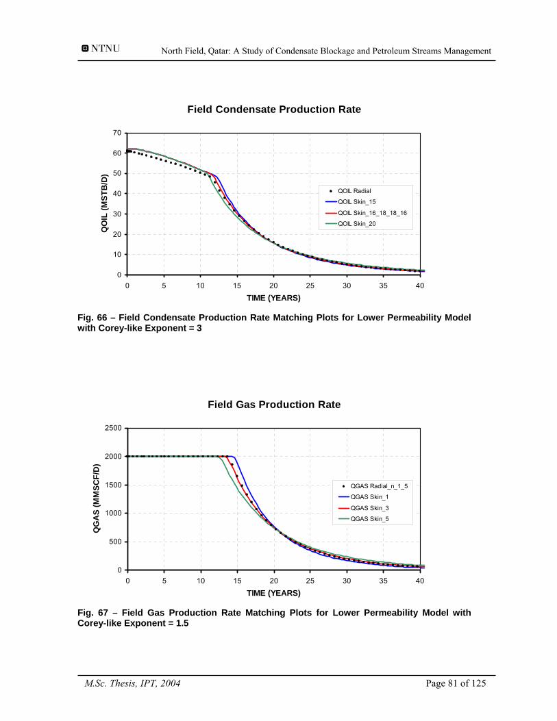
North Field, Qatar: A Study of Condensate Blockage and Petroleum Streams Management
Field Condensate Production Rate
0
10
20
30
40
50
60
70
0 5 10 15 20 25 30 35 40
TIME (YEARS)
QO
IL (M
STB
/D)
QOIL Radial
QOIL Skin_15
QOIL Skin_16_18_18_16
QOIL Skin_20
Fig. 66 – Field Condensate Production Rate Matching Plots for Lower Permeability Model with Corey-like Exponent = 3
Field Gas Production Rate
0
500
1000
1500
2000
2500
0 5 10 15 20 25 30 35 40
TIME (YEARS)
QG
AS
(MM
SCF/
D)
QGAS Radial_n_1_5
QGAS Skin_1
QGAS Skin_3
QGAS Skin_5
Fig. 67 – Field Gas Production Rate Matching Plots for Lower Permeability Model with Corey-like Exponent = 1.5
M.Sc. Thesis, IPT, 2004 Page 81 of 125
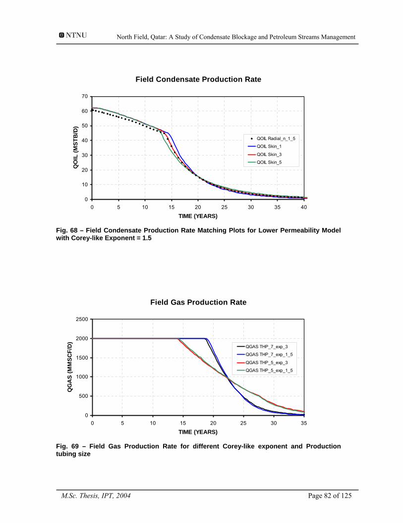
North Field, Qatar: A Study of Condensate Blockage and Petroleum Streams Management
Field Condensate Production Rate
0
10
20
30
40
50
60
70
0 5 10 15 20 25 30 35 40
TIME (YEARS)
QO
IL (M
STB
/D)
QOIL Radial_n_1_5
QOIL Skin_1
QOIL Skin_3
QOIL Skin_5
Fig. 68 – Field Condensate Production Rate Matching Plots for Lower Permeability Model with Corey-like Exponent = 1.5
Field Gas Production Rate
0
500
1000
1500
2000
2500
0 5 10 15 20 25 30 35
TIME (YEARS)
QG
AS
(MM
SCF/
D)
QGAS THP_7_exp_3
QGAS THP_7_exp_1_5
QGAS THP_5_exp_3
QGAS THP_5_exp_1_5
Fig. 69 – Field Gas Production Rate for different Corey-like exponent and Production tubing size
M.Sc. Thesis, IPT, 2004 Page 82 of 125
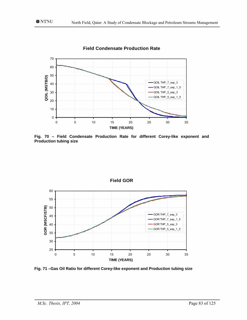
North Field, Qatar: A Study of Condensate Blockage and Petroleum Streams Management
Field Condensate Production Rate
0
10
20
30
40
50
60
70
0 5 10 15 20 25 30 35
TIME (YEARS)
QO
IL (M
STB
/D)
QOIL THP_7_exp_3
QOIL THP_7_exp_1_5
QOIL THP_5_exp_3
QOIL THP_5_exp_1_5
Fig. 70 – Field Condensate Production Rate for different Corey-like exponent and Production tubing size
Field GOR
25
30
35
40
45
50
55
60
0 5 10 15 20 25 30 35
TIME (YEARS)
GO
R (M
SCF/
STB
)
GOR THP_7_exp_3
GOR THP_7_exp_1_5
GOR THP_5_exp_3
GOR THP_5_exp_1_5
Fig. 71 –Gas Oil Ratio for different Corey-like exponent and Production tubing size
M.Sc. Thesis, IPT, 2004 Page 83 of 125
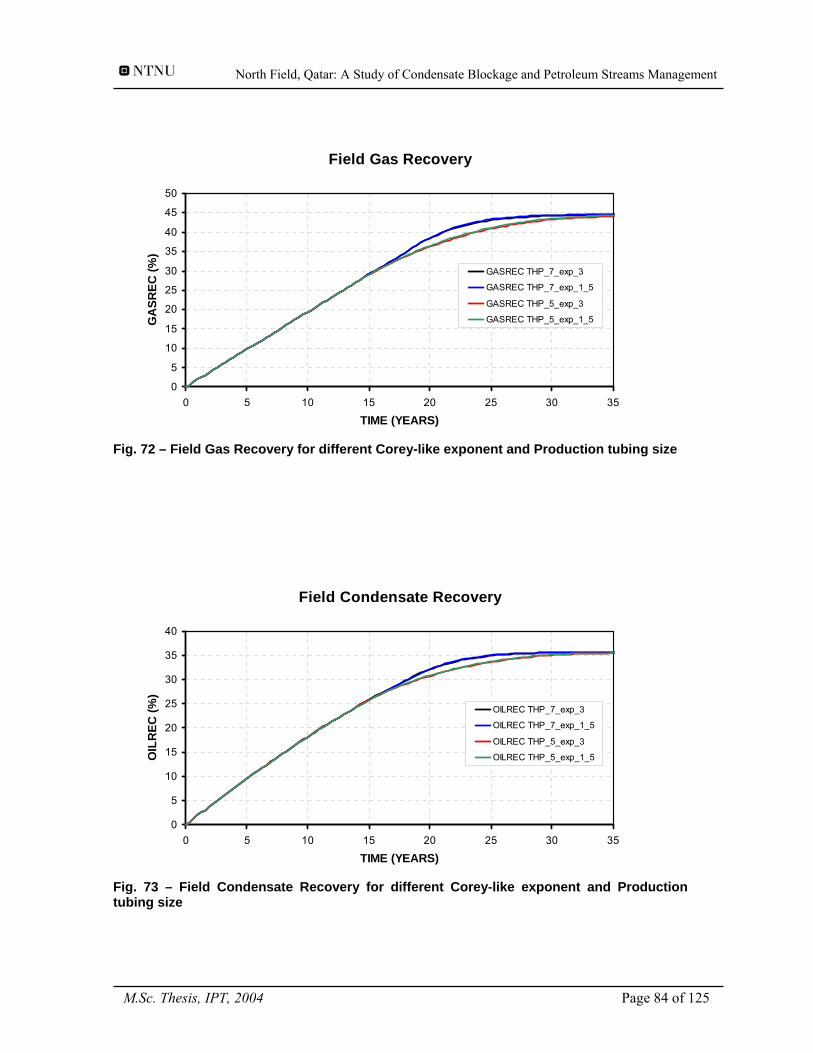
North Field, Qatar: A Study of Condensate Blockage and Petroleum Streams Management
Field Gas Recovery
0
5
10
15
20
25
30
35
40
45
50
0 5 10 15 20 25 30 35
TIME (YEARS)
GA
SREC
(%)
GASREC THP_7_exp_3
GASREC THP_7_exp_1_5
GASREC THP_5_exp_3
GASREC THP_5_exp_1_5
Fig. 72 – Field Gas Recovery for different Corey-like exponent and Production tubing size
Field Condensate Recovery
0
5
10
15
20
25
30
35
40
0 5 10 15 20 25 30 35
TIME (YEARS)
OIL
REC
(%)
OILREC THP_7_exp_3
OILREC THP_7_exp_1_5
OILREC THP_5_exp_3
OILREC THP_5_exp_1_5
Fig. 73 – Field Condensate Recovery for different Corey-like exponent and Production tubing size
M.Sc. Thesis, IPT, 2004 Page 84 of 125
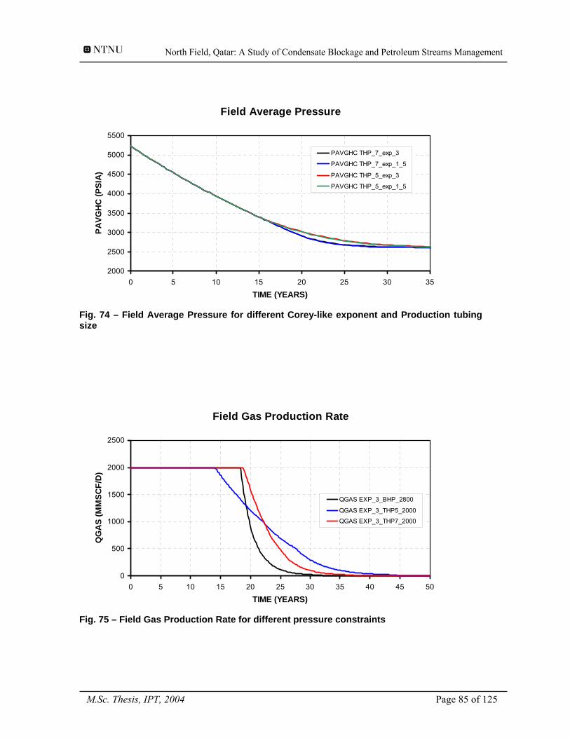
North Field, Qatar: A Study of Condensate Blockage and Petroleum Streams Management
Field Average Pressure
2000
2500
3000
3500
4000
4500
5000
5500
0 5 10 15 20 25 30 35
TIME (YEARS)
PAVG
HC
(PSI
A)
PAVGHC THP_7_exp_3
PAVGHC THP_7_exp_1_5
PAVGHC THP_5_exp_3
PAVGHC THP_5_exp_1_5
Fig. 74 – Field Average Pressure for different Corey-like exponent and Production tubing size
Field Gas Production Rate
0
500
1000
1500
2000
2500
0 5 10 15 20 25 30 35 40 45 50
TIME (YEARS)
QG
AS
(MM
SCF/
D)
QGAS EXP_3_BHP_2800
QGAS EXP_3_THP5_2000
QGAS EXP_3_THP7_2000
Fig. 75 – Field Gas Production Rate for different pressure constraints
M.Sc. Thesis, IPT, 2004 Page 85 of 125
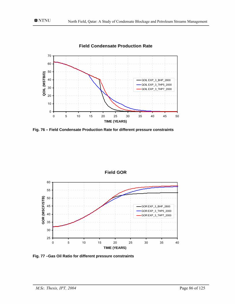
North Field, Qatar: A Study of Condensate Blockage and Petroleum Streams Management
Field Condensate Production Rate
0
10
20
30
40
50
60
70
0 5 10 15 20 25 30 35 40 45 50
TIME (YEARS)
QO
IL (M
STB
/D)
QOIL EXP_3_BHP_2800
QOIL EXP_3_THP5_2000
QOIL EXP_3_THP7_2000
Fig. 76 – Field Condensate Production Rate for different pressure constraints
Field GOR
25
30
35
40
45
50
55
60
0 5 10 15 20 25 30 35 40
TIME (YEARS)
GO
R (M
SCF/
STB
)
GOR EXP_3_BHP_2800
GOR EXP_3_THP5_2000
GOR EXP_3_THP7_2000
Fig. 77 –Gas Oil Ratio for different pressure constraints
M.Sc. Thesis, IPT, 2004 Page 86 of 125
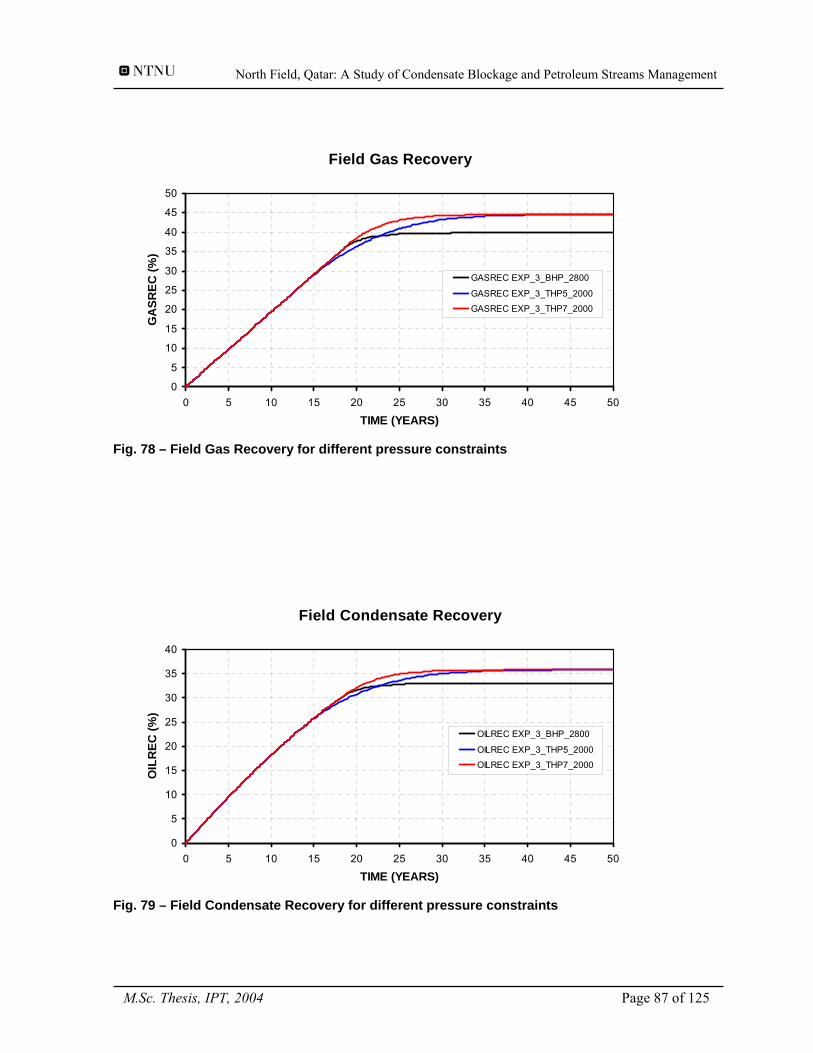
North Field, Qatar: A Study of Condensate Blockage and Petroleum Streams Management
Field Gas Recovery
0
5
10
15
20
25
30
35
40
45
50
0 5 10 15 20 25 30 35 40 45 50
TIME (YEARS)
GA
SREC
(%)
GASREC EXP_3_BHP_2800
GASREC EXP_3_THP5_2000
GASREC EXP_3_THP7_2000
Fig. 78 – Field Gas Recovery for different pressure constraints
Field Condensate Recovery
0
5
10
15
20
25
30
35
40
0 5 10 15 20 25 30 35 40 45 50
TIME (YEARS)
OIL
REC
(%)
OILREC EXP_3_BHP_2800
OILREC EXP_3_THP5_2000
OILREC EXP_3_THP7_2000
Fig. 79 – Field Condensate Recovery for different pressure constraints
M.Sc. Thesis, IPT, 2004 Page 87 of 125
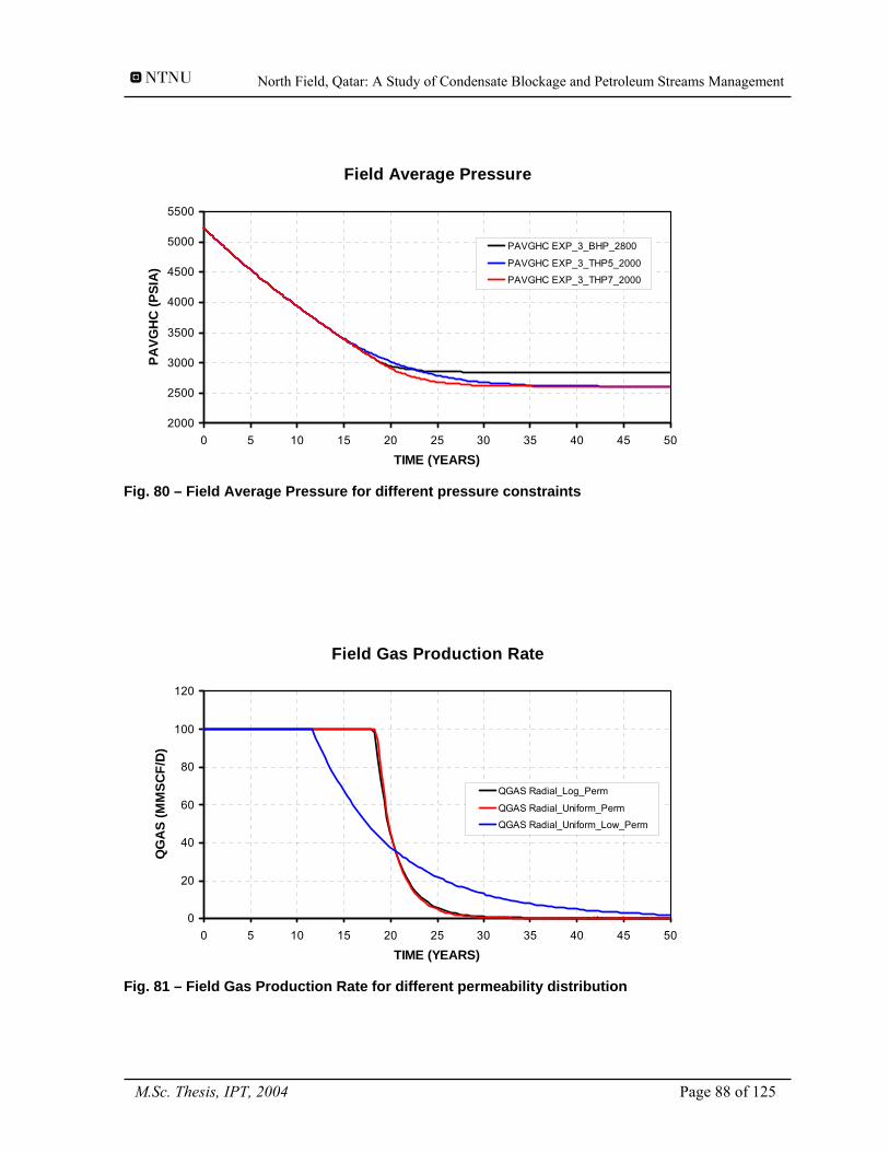
North Field, Qatar: A Study of Condensate Blockage and Petroleum Streams Management
Field Average Pressure
2000
2500
3000
3500
4000
4500
5000
5500
0 5 10 15 20 25 30 35 40 45 50
TIME (YEARS)
PAVG
HC
(PSI
A)
PAVGHC EXP_3_BHP_2800
PAVGHC EXP_3_THP5_2000
PAVGHC EXP_3_THP7_2000
Fig. 80 – Field Average Pressure for different pressure constraints
Field Gas Production Rate
0
20
40
60
80
100
120
0 5 10 15 20 25 30 35 40 45 50
TIME (YEARS)
QG
AS
(MM
SCF/
D)
QGAS Radial_Log_Perm
QGAS Radial_Uniform_Perm
QGAS Radial_Uniform_Low_Perm
Fig. 81 – Field Gas Production Rate for different permeability distribution
M.Sc. Thesis, IPT, 2004 Page 88 of 125
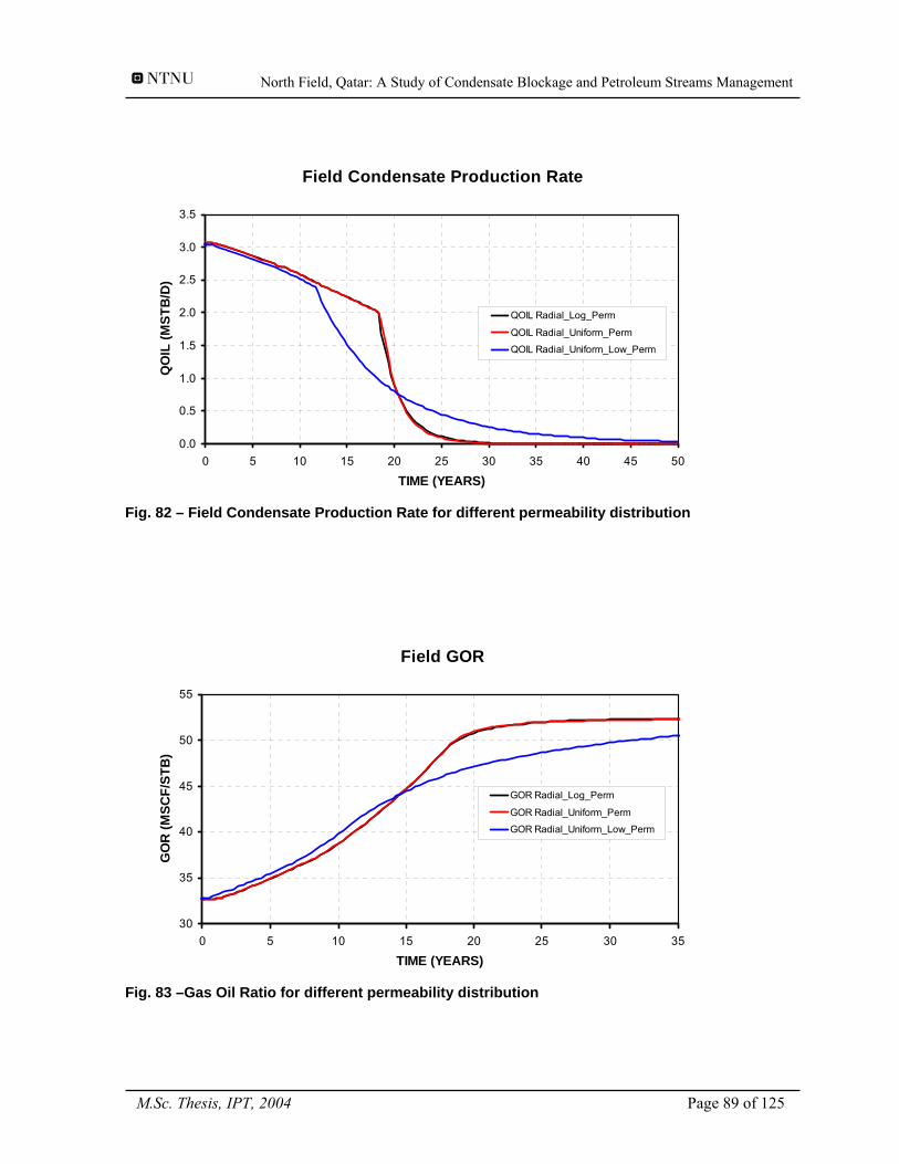
North Field, Qatar: A Study of Condensate Blockage and Petroleum Streams Management
Field Condensate Production Rate
0.0
0.5
1.0
1.5
2.0
2.5
3.0
3.5
0 5 10 15 20 25 30 35 40 45 50
TIME (YEARS)
QO
IL (M
STB
/D)
QOIL Radial_Log_Perm
QOIL Radial_Uniform_Perm
QOIL Radial_Uniform_Low_Perm
Fig. 82 – Field Condensate Production Rate for different permeability distribution
Field GOR
30
35
40
45
50
55
0 5 10 15 20 25 30 35
TIME (YEARS)
GO
R (M
SCF/
STB
)
GOR Radial_Log_Perm
GOR Radial_Uniform_Perm
GOR Radial_Uniform_Low_Perm
Fig. 83 –Gas Oil Ratio for different permeability distribution
M.Sc. Thesis, IPT, 2004 Page 89 of 125
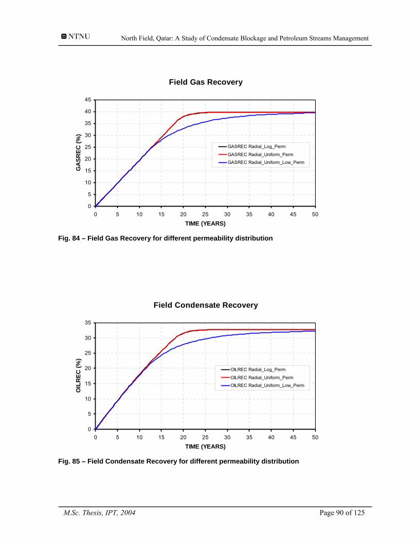
North Field, Qatar: A Study of Condensate Blockage and Petroleum Streams Management
Field Gas Recovery
0
5
10
15
20
25
30
35
40
45
0 5 10 15 20 25 30 35 40 45 50
TIME (YEARS)
GA
SREC
(%)
GASREC Radial_Log_Perm
GASREC Radial_Uniform_Perm
GASREC Radial_Uniform_Low_Perm
Fig. 84 – Field Gas Recovery for different permeability distribution
Field Condensate Recovery
0
5
10
15
20
25
30
35
0 5 10 15 20 25 30 35 40 45 50
TIME (YEARS)
OIL
REC
(%)
OILREC Radial_Log_Perm
OILREC Radial_Uniform_Perm
OILREC Radial_Uniform_Low_Perm
Fig. 85 – Field Condensate Recovery for different permeability distribution
M.Sc. Thesis, IPT, 2004 Page 90 of 125
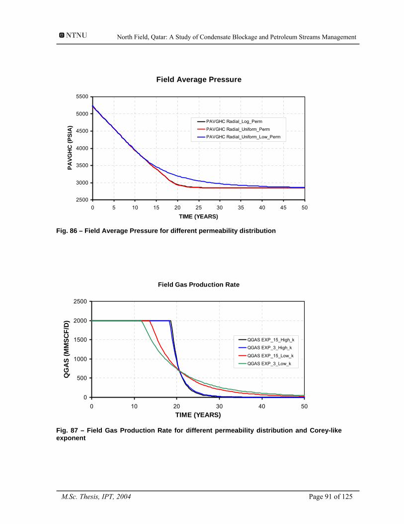
North Field, Qatar: A Study of Condensate Blockage and Petroleum Streams Management
Field Average Pressure
2500
3000
3500
4000
4500
5000
5500
0 5 10 15 20 25 30 35 40 45 50
TIME (YEARS)
PAVG
HC
(PSI
A)
PAVGHC Radial_Log_Perm
PAVGHC Radial_Uniform_Perm
PAVGHC Radial_Uniform_Low_Perm
Fig. 86 – Field Average Pressure for different permeability distribution
Field Gas Production Rate
0
500
1000
1500
2000
2500
0 10 20 30 40 50TIME (YEARS)
QG
AS
(MM
SCF/
D)
QGAS EXP_15_High_k
QGAS EXP_3_High_k
QGAS EXP_15_Low_k
QGAS EXP_3_Low_k
Fig. 87 – Field Gas Production Rate for different permeability distribution and Corey-like exponent
M.Sc. Thesis, IPT, 2004 Page 91 of 125
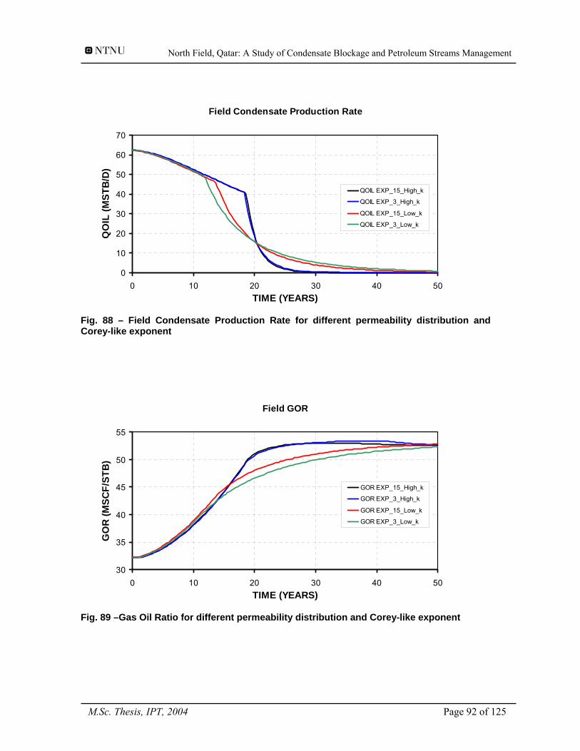
North Field, Qatar: A Study of Condensate Blockage and Petroleum Streams Management
Field Condensate Production Rate
0
10
20
30
40
50
60
70
0 10 20 30 40 50TIME (YEARS)
QO
IL (M
STB
/D)
QOIL EXP_15_High_k
QOIL EXP_3_High_k
QOIL EXP_15_Low_k
QOIL EXP_3_Low_k
Fig. 88 – Field Condensate Production Rate for different permeability distribution and Corey-like exponent
Field GOR
30
35
40
45
50
55
0 10 20 30 40 50TIME (YEARS)
GO
R (M
SCF/
STB
)
GOR EXP_15_High_k
GOR EXP_3_High_k
GOR EXP_15_Low_k
GOR EXP_3_Low_k
Fig. 89 –Gas Oil Ratio for different permeability distribution and Corey-like exponent
M.Sc. Thesis, IPT, 2004 Page 92 of 125
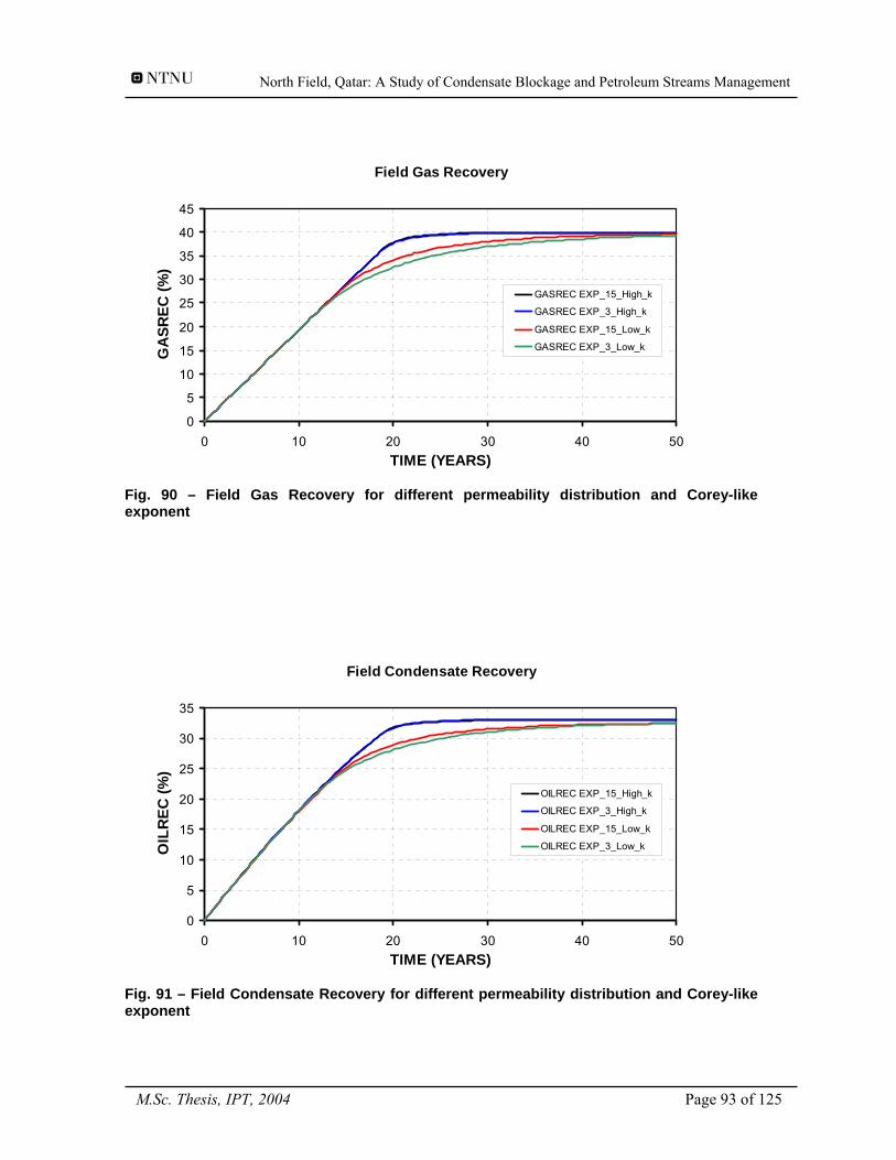
North Field, Qatar: A Study of Condensate Blockage and Petroleum Streams Management
Field Gas Recovery
0
5
10
15
20
25
30
35
40
45
0 10 20 30 40 50TIME (YEARS)
GA
SREC
(%)
GASREC EXP_15_High_k
GASREC EXP_3_High_k
GASREC EXP_15_Low_k
GASREC EXP_3_Low_k
Fig. 90 – Field Gas Recovery for different permeability distribution and Corey-like exponent
Field Condensate Recovery
0
5
10
15
20
25
30
35
0 10 20 30 40 50TIME (YEARS)
OIL
REC
(%)
OILREC EXP_15_High_k
OILREC EXP_3_High_k
OILREC EXP_15_Low_k
OILREC EXP_3_Low_k
Fig. 91 – Field Condensate Recovery for different permeability distribution and Corey-like exponent
M.Sc. Thesis, IPT, 2004 Page 93 of 125
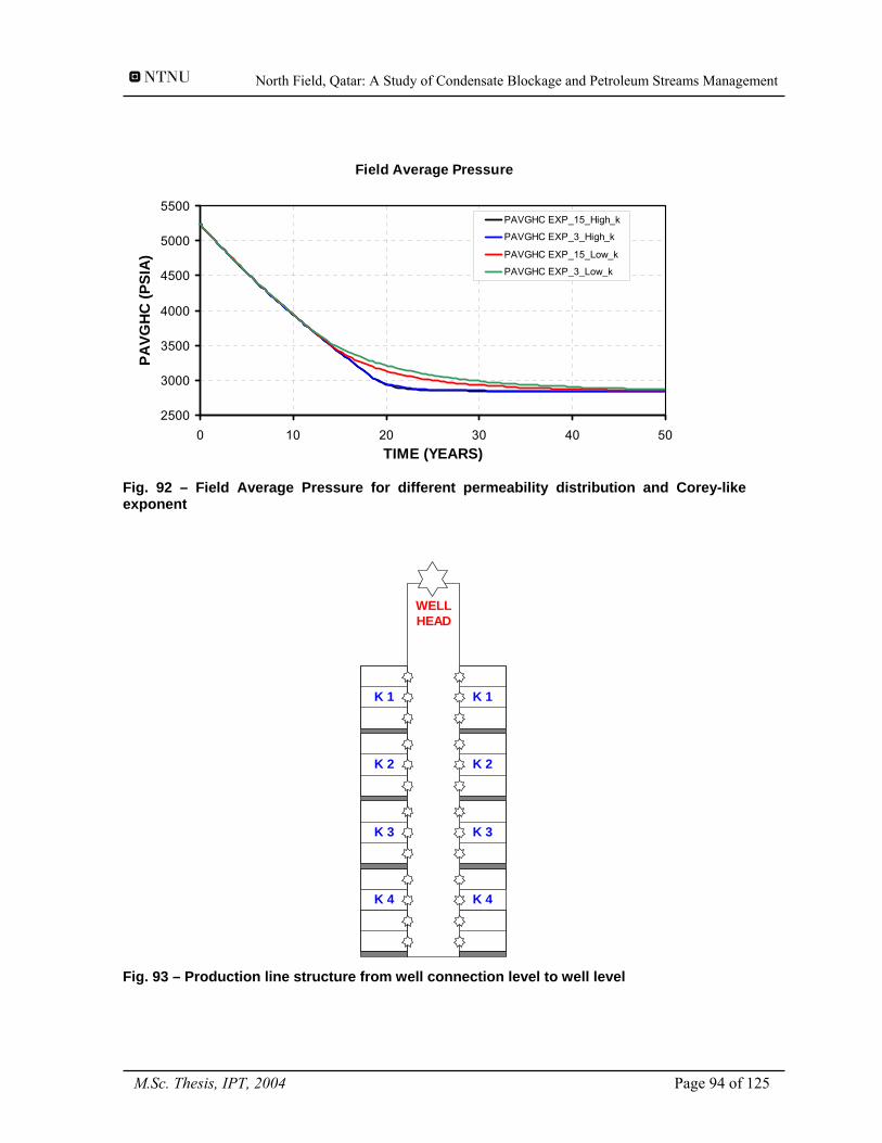
North Field, Qatar: A Study of Condensate Blockage and Petroleum Streams Management
Field Average Pressure
2500
3000
3500
4000
4500
5000
5500
0 10 20 30 40 50TIME (YEARS)
PAVG
HC
(PSI
A)
PAVGHC EXP_15_High_k
PAVGHC EXP_3_High_k
PAVGHC EXP_15_Low_k
PAVGHC EXP_3_Low_k
Fig. 92 – Field Average Pressure for different permeability distribution and Corey-like exponent
K 1
K 2
K 3
K 4
K 1
K 2
K 3
K 4
WELLHEAD
Fig. 93 – Production line structure from well connection level to well level
M.Sc. Thesis, IPT, 2004 Page 94 of 125
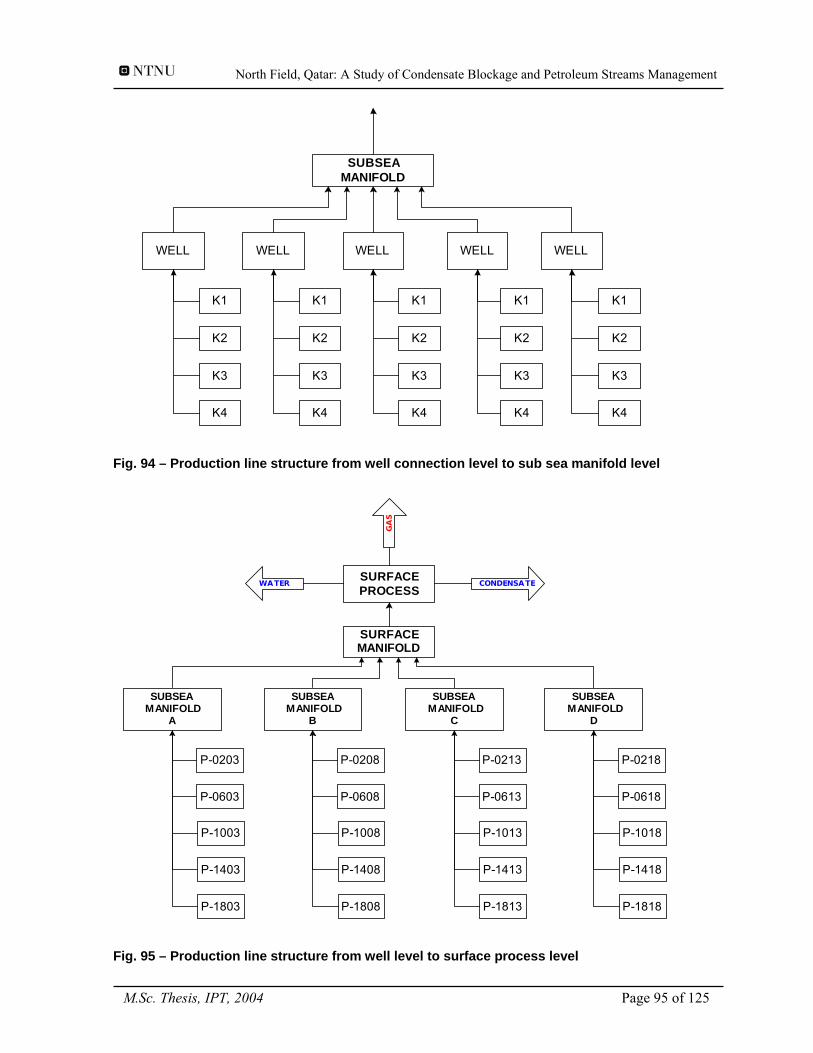
North Field, Qatar: A Study of Condensate Blockage and Petroleum Streams Management
WELL
K1
K2
K3
K4
WELL
K1
K2
K3
K4
WELL
K1
K2
K3
K4
WELL
K1
K2
K3
K4
SUBSEAMANIFOLD
WELL
K1
K2
K3
K4
Fig. 94 – Production line structure from well connection level to sub sea manifold level
SURFACEMANIFOLD
SUBSEAMANIFOLD
A
P-0203
P-0603
P-1003
P-1403
P-1803
SUBSEAMANIFOLD
B
P-0208
P-0608
P-1008
P-1408
P-1808
SUBSEAMANIFOLD
C
P-0213
P-0613
P-1013
P-1413
P-1813
SUBSEAMANIFOLD
D
P-0218
P-0618
P-1018
P-1418
P-1818
SURFACEPROCESS
GAS
CONDENSATEWATER
Fig. 95 – Production line structure from well level to surface process level
M.Sc. Thesis, IPT, 2004 Page 95 of 125
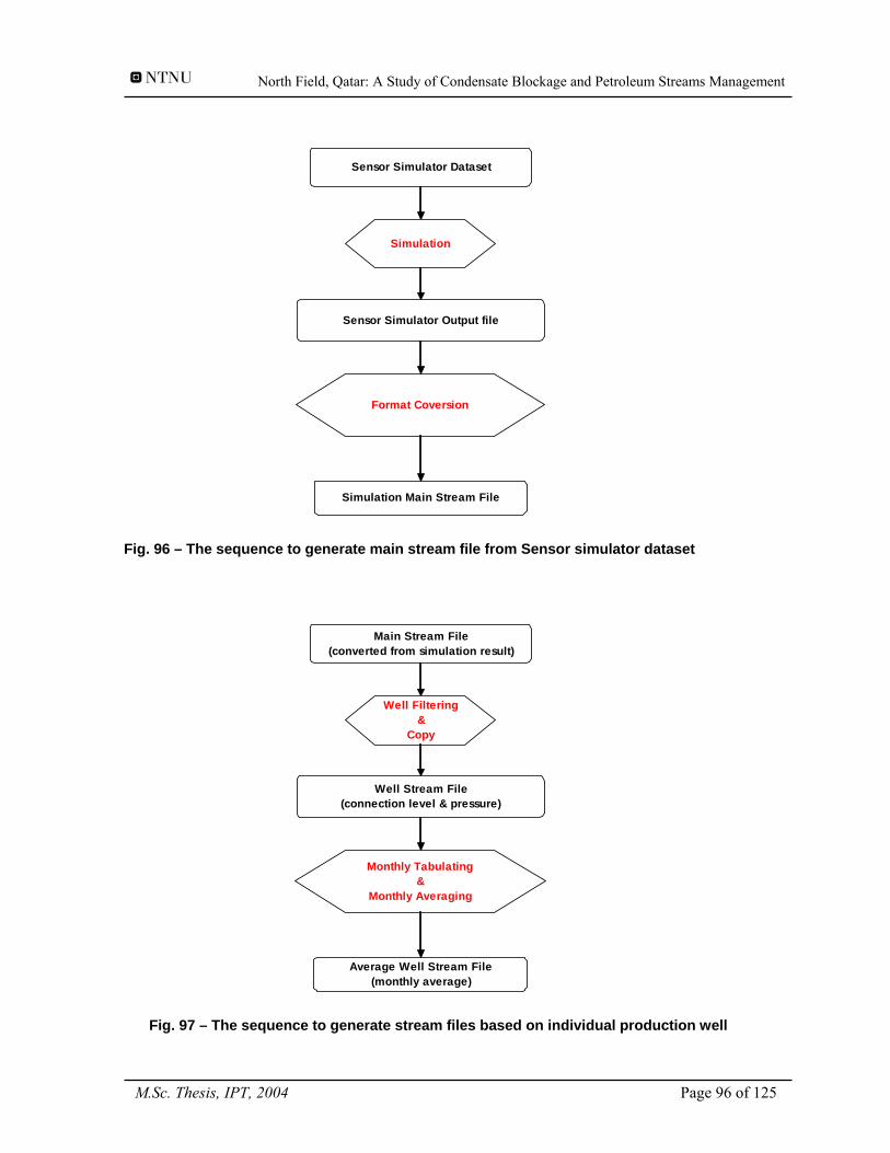
North Field, Qatar: A Study of Condensate Blockage and Petroleum Streams Management
Sensor Simulator Dataset
Sensor Simulator Output file
Simulation
Format Coversion
Simulation Main Stream File
Fig. 96 – The sequence to generate main stream file from Sensor simulator dataset
Main Stream File (converted from simulation result)
Well Stream File (connection level & pressure)
Well Filtering&
Copy
Monthly Tabulating &
Monthly Averaging
Average Well Stream File (monthly average)
Fig. 97 – The sequence to generate stream files based on individual production well
M.Sc. Thesis, IPT, 2004 Page 96 of 125
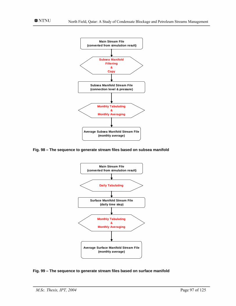
North Field, Qatar: A Study of Condensate Blockage and Petroleum Streams Management
Main Stream File (converted from simulation result)
Subsea Manifold Stream File (connection level & pressure)
Subsea Manifold Filtering
&Copy
Monthly Tabulating &
Monthly Averaging
Average Subsea Manifold Stream File (monthly average)
Fig. 98 – The sequence to generate stream files based on subsea manifold
Main Stream File (converted from simulation result)
Surface Manifold Stream File (daily time step)
Daily Tabulating
Monthly Tabulating &
Monthly Averaging
Average Surface Manifold Stream File (monthly average)
Fig. 99 – The sequence to generate stream files based on surface manifold
M.Sc. Thesis, IPT, 2004 Page 97 of 125
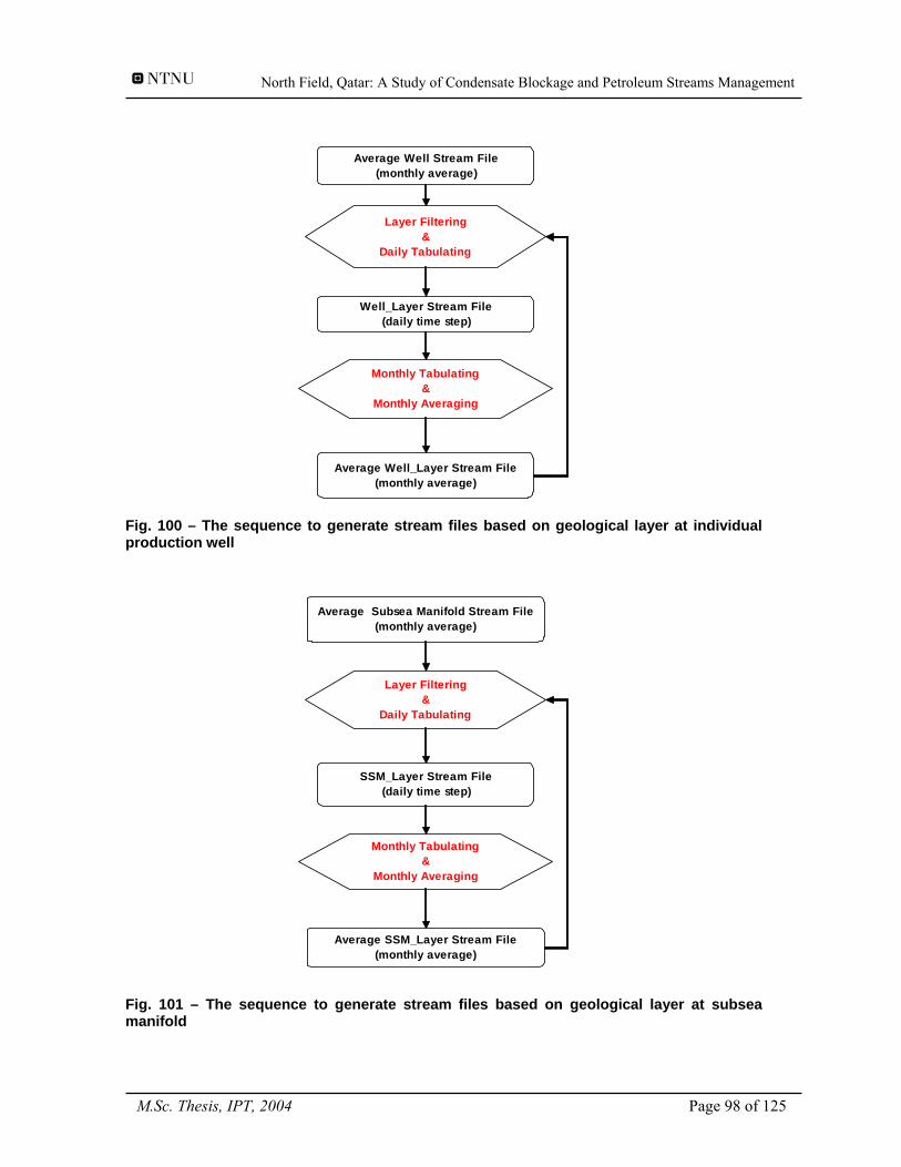
North Field, Qatar: A Study of Condensate Blockage and Petroleum Streams Management
Average Well Stream File (monthly average)
Well_Layer Stream File (daily time step)
Layer Filtering&
Daily Tabulating
Monthly Tabulating &
Monthly Averaging
Average Well_Layer Stream File (monthly average)
Fig. 100 – The sequence to generate stream files based on geological layer at individual production well
Average Subsea Manifold Stream File (monthly average)
SSM_Layer Stream File (daily time step)
Layer Filtering&
Daily Tabulating
Monthly Tabulating &
Monthly Averaging
Average SSM_Layer Stream File (monthly average)
Fig. 101 – The sequence to generate stream files based on geological layer at subsea manifold
M.Sc. Thesis, IPT, 2004 Page 98 of 125
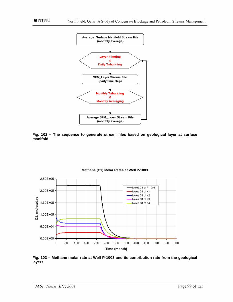
North Field, Qatar: A Study of Condensate Blockage and Petroleum Streams Management
Average Surface Manifold Stream File (monthly average)
SFM_Layer Stream File (daily time step)
Layer Filtering&
Daily Tabulating
Monthly Tabulating &
Monthly Averaging
Average SFM_Layer Stream File (monthly average)
Fig. 102 – The sequence to generate stream files based on geological layer at surface manifold
Methane (C1) Molar Rates at Well P-1003
0.00E+00
5.00E+04
1.00E+05
1.50E+05
2.00E+05
2.50E+05
0 50 100 150 200 250 300 350 400 450 500 550 600
Time (month)
C1,
mol
es/d
ay
Moles C1 of P-1003Moles C1 of K1Moles C1 of K2Moles C1 of K3Moles C1 of K4
Fig. 103 – Methane molar rate at Well P-1003 and its contribution rate from the geological layers
M.Sc. Thesis, IPT, 2004 Page 99 of 125
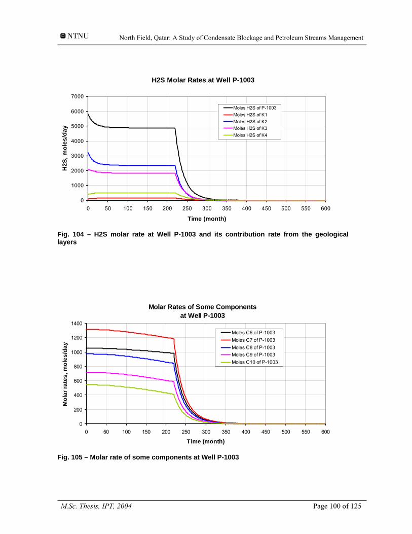
North Field, Qatar: A Study of Condensate Blockage and Petroleum Streams Management
H2S Molar Rates at Well P-1003
0
1000
2000
3000
4000
5000
6000
7000
0 50 100 150 200 250 300 350 400 450 500 550 600
Time (month)
H2S
, mol
es/d
ay
Moles H2S of P-1003Moles H2S of K1Moles H2S of K2Moles H2S of K3Moles H2S of K4
Fig. 104 – H2S molar rate at Well P-1003 and its contribution rate from the geological layers
Molar Rates of Some Components at Well P-1003
0
200
400
600
800
1000
1200
1400
0 50 100 150 200 250 300 350 400 450 500 550 600
Time (month)
Mol
ar ra
tes,
mol
es/d
ay
Moles C6 of P-1003Moles C7 of P-1003Moles C8 of P-1003Moles C9 of P-1003Moles C10 of P-1003
Fig. 105 – Molar rate of some components at Well P-1003
M.Sc. Thesis, IPT, 2004 Page 100 of 125
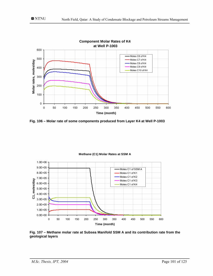
North Field, Qatar: A Study of Condensate Blockage and Petroleum Streams Management
Component Molar Rates of K4 at Well P-1003
0
100
200
300
400
500
600
0 50 100 150 200 250 300 350 400 450 500 550 600
Time (month)
Mol
ar ra
tes,
mol
es/d
ay
Moles C6 of K4Moles C7 of K4Moles C8 of K4Moles C9 of K4Moles C10 of K4
Fig. 106 – Molar rate of some components produced from Layer K4 at Well P-1003
Methane (C1) Molar Rates at SSM A
0.0E+00
1.0E+05
2.0E+05
3.0E+05
4.0E+05
5.0E+05
6.0E+05
7.0E+05
8.0E+05
9.0E+05
1.0E+06
0 50 100 150 200 250 300 350 400 450 500 550 600
Time (month)
C1,
mol
es/d
ay
Moles C1 of SSM AMoles C1 of K1Moles C1 of K2Moles C1 of K3Moles C1 of K4
Fig. 107 – Methane molar rate at Subsea Manifold SSM A and its contribution rate from the geological layers
M.Sc. Thesis, IPT, 2004 Page 101 of 125
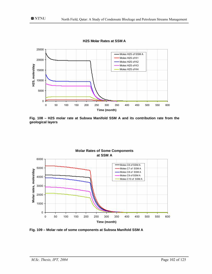
North Field, Qatar: A Study of Condensate Blockage and Petroleum Streams Management
H2S Molar Rates at SSM A
0
5000
10000
15000
20000
25000
0 50 100 150 200 250 300 350 400 450 500 550 600
Time (month)
H2S
, mol
es/d
ay
Moles H2S of SSM AMoles H2S of K1Moles H2S of K2Moles H2S of K3Moles H2S of K4
Fig. 108 – H2S molar rate at Subsea Manifold SSM A and its contribution rate from the geological layers
Molar Rates of Some Components at SSM A
0
1000
2000
3000
4000
5000
6000
0 50 100 150 200 250 300 350 400 450 500 550 600
Time (month)
Mol
ar ra
tes,
mol
es/d
ay
Moles C6 of SSM AMoles C7 of SSM AMoles C8 of SSM AMoles C9 of SSM AMoles C10 of SSM A
Fig. 109 – Molar rate of some components at Subsea Manifold SSM A
M.Sc. Thesis, IPT, 2004 Page 102 of 125
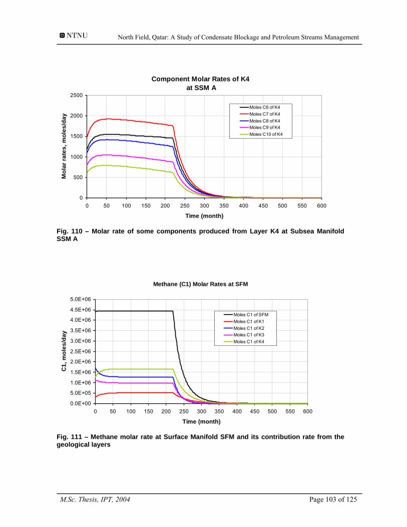
North Field, Qatar: A Study of Condensate Blockage and Petroleum Streams Management
Component Molar Rates of K4 at SSM A
0
500
1000
1500
2000
2500
0 50 100 150 200 250 300 350 400 450 500 550 600
Time (month)
Mol
ar ra
tes,
mol
es/d
ay
Moles C6 of K4Moles C7 of K4Moles C8 of K4Moles C9 of K4Moles C10 of K4
Fig. 110 – Molar rate of some components produced from Layer K4 at Subsea Manifold SSM A
Methane (C1) Molar Rates at SFM
0.0E+00
5.0E+05
1.0E+06
1.5E+06
2.0E+06
2.5E+06
3.0E+06
3.5E+06
4.0E+06
4.5E+06
5.0E+06
0 50 100 150 200 250 300 350 400 450 500 550 600
Time (month)
C1,
mol
es/d
ay
Moles C1 of SFMMoles C1 of K1Moles C1 of K2Moles C1 of K3Moles C1 of K4
Fig. 111 – Methane molar rate at Surface Manifold SFM and its contribution rate from the geological layers
M.Sc. Thesis, IPT, 2004 Page 103 of 125
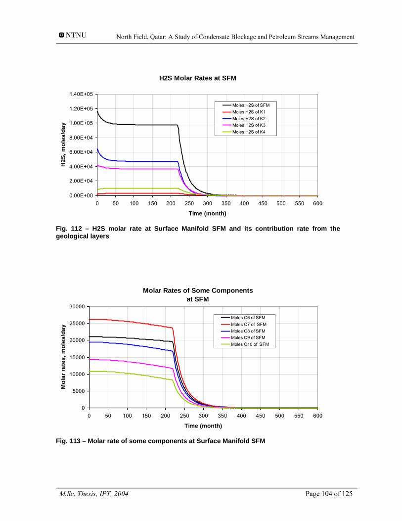
North Field, Qatar: A Study of Condensate Blockage and Petroleum Streams Management
H2S Molar Rates at SFM
0.00E+00
2.00E+04
4.00E+04
6.00E+04
8.00E+04
1.00E+05
1.20E+05
1.40E+05
0 50 100 150 200 250 300 350 400 450 500 550 600
Time (month)
H2S
, mol
es/d
ay
Moles H2S of SFMMoles H2S of K1Moles H2S of K2Moles H2S of K3Moles H2S of K4
Fig. 112 – H2S molar rate at Surface Manifold SFM and its contribution rate from the geological layers
Molar Rates of Some Components at SFM
0
5000
10000
15000
20000
25000
30000
0 50 100 150 200 250 300 350 400 450 500 550 600
Time (month)
Mol
ar ra
tes,
mol
es/d
ay
Moles C6 of SFMMoles C7 of SFMMoles C8 of SFMMoles C9 of SFMMoles C10 of SFM
Fig. 113 – Molar rate of some components at Surface Manifold SFM
M.Sc. Thesis, IPT, 2004 Page 104 of 125
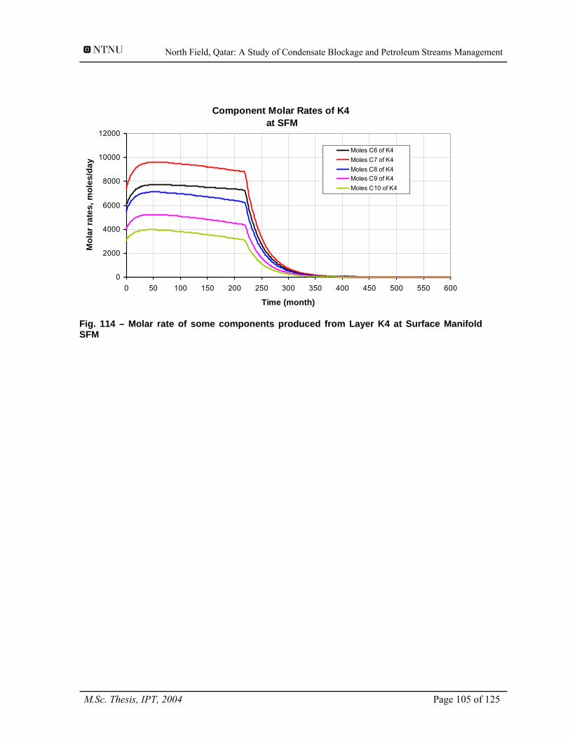
North Field, Qatar: A Study of Condensate Blockage and Petroleum Streams Management
Component Molar Rates of K4 at SFM
0
2000
4000
6000
8000
10000
12000
0 50 100 150 200 250 300 350 400 450 500 550 600
Time (month)
Mol
ar ra
tes,
mol
es/d
ay
Moles C6 of K4Moles C7 of K4Moles C8 of K4Moles C9 of K4Moles C10 of K4
Fig. 114 – Molar rate of some components produced from Layer K4 at Surface Manifold SFM
M.Sc. Thesis, IPT, 2004 Page 105 of 125
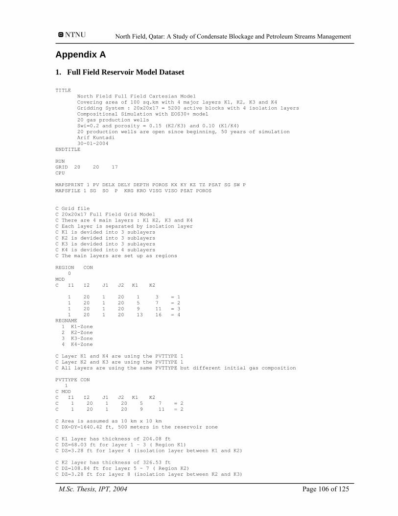
North Field, Qatar: A Study of Condensate Blockage and Petroleum Streams Management
Appendix A
1. Full Field Reservoir Model Dataset TITLE North Field Full Field Cartesian Model Covering area of 100 sq.km with 4 major layers K1, K2, K3 and K4 Gridding System : 20x20x17 = 5200 active blocks with 4 isolation layers Compositional Simulation with EOS30+ model 20 gas production wells Swi=0.2 and porosity = 0.15 (K2/K3) and 0.10 (K1/K4) 20 production wells are open since beginning, 50 years of simulation Arif Kuntadi 30-01-2004 ENDTITLE RUN GRID 20 20 17 CPU MAPSPRINT 1 PV DELX DELY DEPTH POROS KX KY KZ TZ PSAT SG SW P MAPSFILE 1 SG SO P KRG KRO VISG VISO PSAT POROS C Grid file C 20x20x17 Full Field Grid Model C There are 4 main layers : K1 K2, K3 and K4 C Each layer is separated by isolation layer C K1 is devided into 3 sublayers C K2 is devided into 3 sublayers C K3 is devided into 3 sublayers C K4 is devided into 4 sublayers C The main layers are set up as regions REGION CON 0 MOD C I1 I2 J1 J2 K1 K2 1 20 1 20 1 3 = 1 1 20 1 20 5 7 = 2 1 20 1 20 9 11 = 3 1 20 1 20 13 16 = 4 REGNAME 1 K1-Zone 2 K2-Zone 3 K3-Zone 4 K4-Zone C Layer K1 and K4 are using the PVTTYPE 1 C Layer K2 and K3 are using the PVTTYPE 1 C All layers are using the same PVTTYPE but different initial gas composition PVTTYPE CON 1 C MOD C I1 I2 J1 J2 K1 K2 C 1 20 1 20 5 7 = 2 C 1 20 1 20 9 11 = 2 C Area is assumed as 10 km x 10 km C DX=DY=1640.42 ft, 500 meters in the reservoir zone C K1 layer has thickness of 204.08 ft C DZ=68.03 ft for layer 1 - 3 ( Region K1) C DZ=3.28 ft for layer 4 (isolation layer between K1 and K2) C K2 layer has thickness of 326.53 ft C DZ=108.84 ft for layer 5 - 7 ( Region K2) C DZ=3.28 ft for layer 8 (isolation layer between K2 and K3)
M.Sc. Thesis, IPT, 2004 Page 106 of 125
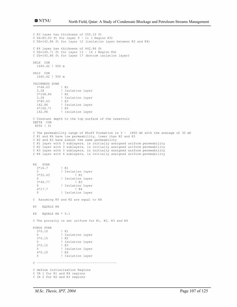
North Field, Qatar: A Study of Condensate Blockage and Petroleum Streams Management
C K3 layer has thickness of 255.10 ft C DZ=85.03 ft for layer 9 - 11 ( Region K3) C DZ=142.86 ft for layer 12 (isolation layer between K3 and K4) C K4 layer has thickness of 642.86 ft C DZ=160.71 ft for layer 13 - 16 ( Region K4) C DZ=142.86 ft for layer 17 (bottom isolation layer) DELX CON 1640.42 ! 500 m DELY CON 1640.42 ! 500 m THICKNESS ZVAR 3*68.03 ! K1 3.28 ! Isolation layer 3*108.84 ! K2 3.28 ! Isolation layer 3*85.03 ! K3 142.86 ! Isolation layer 4*160.71 ! K4 142.86 ! Isolation layer C Constant depth to the top surface of the reservoir DEPTH CON 8050 ! ft C The permeability range of Khuff Formation is 3 - 1800 mD with the average of 30 mD C K1 and K4 have low permeability, lower than K2 and K3 C K2 and K3 have almost the same permeability C K1 layer with 3 sublayers, is initially assigned uniform permeability C K2 layer with 3 sublayers, is initially assigned uniform permeability C K3 layer with 3 sublayers, is initially assigned uniform permeability C K4 layer with 4 sublayers, is initially assigned uniform permeability KX ZVAR 3*16.7 ! K1 0 ! Isolation layer 3*52.43 ! K2 0 ! Isolation layer 3*46.77 ! K3 0 ! Isolation layer 4*17.7 ! K4 0 ! Isolation layer C Assuming KY and KZ are equal to KX KY EQUALS KX KZ EQUALS KX * 0.1 C The porosity is set uniform for K1, K2, K3 and K4 POROS ZVAR 3*0.10 ! K1 0 ! Isolation layer 3*0.15 ! K2 0 ! Isolation layer 3*0.15 ! K3 0 ! Isolation layer 4*0.10 ! K4 0 ! Isolation layer C ------------------------------------------- C define Initialization Regions C IR 1 for K1 and K4 regions C IR 2 for K2 and K3 regions
M.Sc. Thesis, IPT, 2004 Page 107 of 125
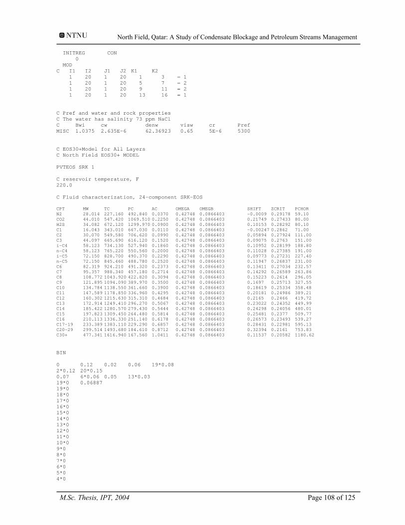
North Field, Qatar: A Study of Condensate Blockage and Petroleum Streams Management
INITREG CON 0 MOD C I1 I2 J1 J2 K1 K2 1 20 1 20 1 3 = 1 1 20 1 20 5 7 = 2 1 20 1 20 9 11 = 2 1 20 1 20 13 16 = 1 C Pref and water and rock properties C The water has salinity 73 ppm NaCl C Bwi cw denw visw cr Pref MISC 1.0375 2.635E-6 62.36923 0.65 5E-6 5300 C EOS30+Model for All Layers C North Field EOS30+ MODEL PVTEOS SRK 1 C reservoir temperature, F 220.0 C Fluid characterization, 24-component SRK-EOS CPT MW TC PC AC OMEGA OMEGB SHIFT ZCRIT PCHOR N2 28.014 227.160 492.840 0.0370 0.42748 0.0866403 -0.0009 0.29178 59.10 CO2 44.010 547.420 1069.510 0.2250 0.42748 0.0866403 0.21749 0.27433 80.00 H2S 34.082 672.120 1299.970 0.0900 0.42748 0.0866403 0.10153 0.28292 80.10 C1 16.043 343.010 667.030 0.0110 0.42748 0.0866403 -0.00247 0.2862 71.00 C2 30.070 549.580 706.620 0.0990 0.42748 0.0866403 0.05894 0.27924 111.00 C3 44.097 665.690 616.120 0.1520 0.42748 0.0866403 0.09075 0.2763 151.00 i-C4 58.123 734.130 527.940 0.1860 0.42748 0.0866403 0.10952 0.28199 188.80 n-C4 58.123 765.220 550.560 0.2000 0.42748 0.0866403 0.11028 0.27385 191.00 i-C5 72.150 828.700 490.370 0.2290 0.42748 0.0866403 0.09773 0.27231 227.40 n-C5 72.150 845.460 488.780 0.2520 0.42748 0.0866403 0.11947 0.26837 231.00 C6 82.319 924.210 491.320 0.2373 0.42748 0.0866403 0.13411 0.27034 232.57 C7 95.357 988.340 457.180 0.2714 0.42748 0.0866403 0.14292 0.26589 263.86 C8 108.772 1043.920 422.820 0.3094 0.42748 0.0866403 0.15223 0.2614 296.05 C9 121.895 1094.090 389.970 0.3500 0.42748 0.0866403 0.1697 0.25713 327.55 C10 134.784 1138.550 361.660 0.3900 0.42748 0.0866403 0.18619 0.25334 358.48 C11 147.589 1178.850 336.960 0.4295 0.42748 0.0866403 0.20181 0.24986 389.21 C12 160.302 1215.630 315.310 0.4684 0.42748 0.0866403 0.2165 0.2466 419.72 C13 172.914 1249.410 296.270 0.5067 0.42748 0.0866403 0.23022 0.24352 449.99 C14 185.422 1280.570 279.430 0.5444 0.42748 0.0866403 0.24298 0.24056 480.01 C15 197.823 1309.450 264.480 0.5814 0.42748 0.0866403 0.25481 0.2377 509.77 C16 210.113 1336.330 251.140 0.6178 0.42748 0.0866403 0.26573 0.23493 539.27 C17-19 233.389 1383.110 229.290 0.6857 0.42748 0.0866403 0.28431 0.22981 595.13 C20-29 299.514 1493.680 184.610 0.8712 0.42748 0.0866403 0.32394 0.2161 753.83 C30+ 477.341 1616.940 167.560 1.0411 0.42748 0.0866403 0.11537 0.20582 1180.62 BIN 0 0.12 0.02 0.06 19*0.08 2*0.12 20*0.15 0.07 6*0.06 0.05 13*0.03 19*0 0.06887 19*0 18*0 17*0 16*0 15*0 14*0 13*0 12*0 11*0 10*0 9*0 8*0 7*0 6*0 5*0 4*0
M.Sc. Thesis, IPT, 2004 Page 108 of 125
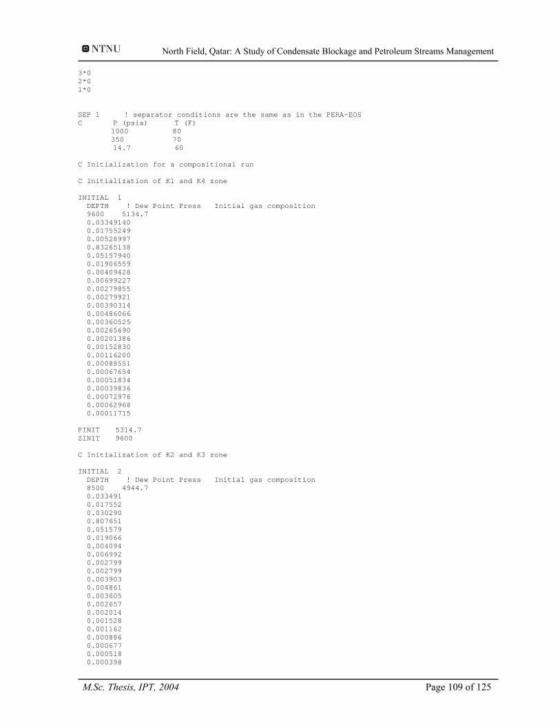
North Field, Qatar: A Study of Condensate Blockage and Petroleum Streams Management
3*0 2*0 1*0 SEP 1 ! separator conditions are the same as in the PERA-EOS C P (psia) T (F) 1000 80 350 70 14.7 60 C Initialization for a compositional run C Initialization of K1 and K4 zone INITIAL 1 DEPTH ! Dew Point Press Initial gas composition 9600 5134.7 0.03349140 0.01755249 0.00528997 0.83265138 0.05157940 0.01906559 0.00409428 0.00699227 0.00279855 0.00279921 0.00390314 0.00486066 0.00360525 0.00265690 0.00201386 0.00152830 0.00116200 0.00088551 0.00067654 0.00051834 0.00039836 0.00072976 0.00062968 0.00011715 PINIT 5314.7 ZINIT 9600 C Initialization of K2 and K3 zone INITIAL 2 DEPTH ! Dew Point Press Initial gas composition 8500 4944.7 0.033491 0.017552 0.030290 0.807651 0.051579 0.019066 0.004094 0.006992 0.002799 0.002799 0.003903 0.004861 0.003605 0.002657 0.002014 0.001528 0.001162 0.000886 0.000677 0.000518 0.000398
M.Sc. Thesis, IPT, 2004 Page 109 of 125
North Field, Qatar: A Study of Condensate Blockage and Petroleum Streams Management
0.000730 0.000630 0.000117 PINIT 5204.7 ZINIT 8500 C Relative Perms C Two-phase water-oil saturation table C Swi=0.2 C Water is wetting phase KRANALYTICAL .2 .2 .2 .1 ! swc sorw sorg sgc .5 .33 .9 ! krwro krgro krocw 3 3 3 3 ! nw now ng nog ENDINIT PSM C ------------------------- Recurrent Data ----------------------------- C Well data C There are 20 production wells C Wells are producing from all layers WELL I J K1 K2 SKIN ! header line calculate well indices internally P-0203 2 3 1 3 17 2 3 5 7 13 2 3 9 11 15 2 3 13 16 12 P-0208 2 8 1 3 17 2 8 5 7 13 2 8 9 11 15 2 8 13 16 12 P-0213 2 13 1 3 17 2 13 5 7 13 2 13 9 11 15 2 13 13 16 12 P-0218 2 18 1 3 17 2 18 5 7 13 2 18 9 11 15 2 18 13 16 12 P-0603 6 3 1 3 17 6 3 5 7 13 6 3 9 11 15 6 3 13 16 12 P-0608 6 8 1 3 17 6 8 5 7 13 6 8 9 11 15 6 8 13 16 12 P-0613 6 13 1 3 17 6 13 5 7 13 6 13 9 11 15 6 13 13 16 12 P-0618 6 18 1 3 17 6 18 5 7 13 6 18 9 11 15 6 18 13 16 12 P-1003 10 3 1 3 17 10 3 5 7 13 10 3 9 11 15
M.Sc. Thesis, IPT, 2004 Page 110 of 125
North Field, Qatar: A Study of Condensate Blockage and Petroleum Streams Management
10 3 13 16 12 P-1008 10 8 1 3 17 10 8 5 7 13 10 8 9 11 15 10 8 13 16 12 P-1013 10 13 1 3 17 10 13 5 7 13 10 13 9 11 15 10 13 13 16 12 P-1018 10 18 1 3 17 10 18 5 7 13 10 18 9 11 15 10 18 13 16 12 P-1403 14 3 1 3 17 14 3 5 7 13 14 3 9 11 15 14 3 13 16 12 P-1408 14 8 1 3 17 14 8 5 7 13 14 8 9 11 15 14 8 13 16 12 P-1413 14 13 1 3 17 14 13 5 7 13 14 13 9 11 15 14 13 13 16 12 P-1418 14 18 1 3 17 14 18 5 7 13 14 18 9 11 15 14 18 13 16 12 P-1803 18 3 1 3 17 18 3 5 7 13 18 3 9 11 15 18 3 13 16 12 P-1808 18 8 1 3 17 18 8 5 7 13 18 8 9 11 15 18 8 13 16 12 P-1813 18 13 1 3 17 18 13 5 7 13 18 13 9 11 15 18 13 13 16 12 P-1818 18 18 1 3 17 18 18 5 7 13 18 18 9 11 15 18 18 13 16 12 WELLTYPE P-0203 - P-1818 MCF ! gas producer, Mscf/D WELLPLAT ! assign wells to a particular platform -1 1 ! Assign all gas wells to platform 1 ! "-1" means all producers C Define field production target rate C The Field Target Rate is 2000 MMSCF/D PTARG 1 G 2e6 ! Field plateau rate, MCF/D C Including Tubing Peformance Table with 5.5" Production Tubing
M.Sc. Thesis, IPT, 2004 Page 111 of 125

North Field, Qatar: A Study of Condensate Blockage and Petroleum Streams Management
c include c thp5_5.inc BHP P-0203 - P-1818 2800 ! Minimum Well Bottom Hole Pressure is set to 2800 psia C Initially all 20 wells are open for production C Each well has production rate of 100 MMSCF/D RATE P-0203 - P-1818 100000 ! MCF/D target rate WELLSUM -1 1 ! output summary for all producers PLATSUM -1 0 ! print out platform summary for all timesteps MAPSFILEFREQ 1 TIME 18250 365 END
2. Radial Reservoir Model Dataset TITLE North Field Radial Model with single production well Covering area of 5 sq.km with 4 major layers K1, K2, K3 and K4 Gridding System : 25x17x1 = 3525 active blocks with 4 isolation layers BO Tables are generated internally with EOS30+ model Swi=0.2 and porosity = 15% (K2/K3) and 10% (K1/K4) 50 years of simulation Arif Kuntadi 23-03-2004 ENDTITLE RUN GRID 25 1 145 RUN CPU IMPLICIT MAPSPRINT 1 SG SO P KRG KRO VISG VISO PSAT MAPSFILE 1 SG SO P KRG KRO VISG VISO PSAT C Grid file C 25x17x1 Radial Model C There are 4 main layers : K1 K2, K3 and K4 C Each layer is separated by isolation layer C K1 is devided into 20 sublayers C K2 is devided into 32 sublayers C K3 is devided into 25 sublayers C K4 is devided into 64 sublayers C The main layers are set up as regions REGION CON 0 MOD C I1 I2 J1 J2 K1 K2 1 25 1 1 1 20 = 1 1 25 1 1 22 53 = 2 1 25 1 1 55 79 = 3 1 25 1 1 81 144 = 4 REGNAME 1 K1-Zone
M.Sc. Thesis, IPT, 2004 Page 112 of 125
North Field, Qatar: A Study of Condensate Blockage and Petroleum Streams Management
2 K2-Zone 3 K3-Zone 4 K4-Zone C Layer K1 and K4 are using the PVTTYPE 1 C Layer K2 and K3 are using the PVTTYPE 1 C All layers are using the same PVTTYPE but different initial gas composition PVTTYPE CON 1 C Drainage area was calculated as 1/20 of total area covered in Full Field Model C Drainage area = 5 km2 (5.38E+07 ft2) C Drainage radius (re) = 4140 ft C K1 layer has thickness of 204.08 ft C DZ=10.20 ft for layer 1 - 20 ( Region K1) C DZ=3.28 ft for layer 4 (isolation layer between K1 and K2) C K2 layer has thickness of 326.53 ft C DZ=10.20 ft for layer 21 - 52 ( Region K2) C DZ=3.28 ft for layer 8 (isolation layer between K2 and K3) C K3 layer has thickness of 255.10 ft C DZ=10.20 ft for layer 53 - 77 ( Region K3) C DZ=142.86 ft for layer 12 (isolation layer between K3 and K4) C K4 layer has thickness of 642.86 ft C DZ=10.04 ft for layer 78 - 141 ( Region K4) C DZ=142.86 ft for layer 17 (bottom isolation layer) RADIAL 1 ! grid sizes are generated automatically - equal spacing in log(r) .583 4140 ! well radius = 7" and outer radius of drainage area (re) 360 ! model full 360 deg round well THICKNESS ZVAR 20*10.20 ! K1 3.28 ! Isolation layer 32*10.20 ! K2 3.28 ! Isolation layer 25*10.20 ! K3 142.86 ! Isolation layer 64*10.04 ! K4 142.86 ! Isolation layer C Constant depth to the top surface of the reservoir DEPTH CON 8050 ! ft C The permeability range of Khuff Formation is 3 - 1800 mD with the average of 30 mD C K1 and K4 have low permeability, lower than K2 and K3 C K2 and K3 have almost the same permeability C K1 layer has 20 sublayers with uniform permeability = 16.7 mD C K2 layer has 32 sublayers with uniform permeability = 52.43 mD C K3 layer has 25 sublayers with uniform permeability = 46.77 mD C K4 layer has 64 sublayers with uniform permeability = 17.7 mD KX ZVAR 20*16.7 ! K1 0 ! Isolation layer 32*52.43 ! K2 0 ! Isolation layer 25*46.77 ! K3 0 ! Isolation layer 64*17.7 ! K4 0 ! Isolation layer C Assuming KY and KZ are equal to KX
M.Sc. Thesis, IPT, 2004 Page 113 of 125
North Field, Qatar: A Study of Condensate Blockage and Petroleum Streams Management
KY EQUALS KX KZ EQUALS KX * 0.5 C The porosity is set uniform for K1, K2, K3 and K4 POROS ZVAR 20*0.10 ! K1 0 ! Isolation layer 32*0.15 ! K2 0 ! Isolation layer 25*0.15 ! K3 0 ! Isolation layer 64*0.10 ! K4 0 ! Isolation layer C ------------------------------------------- C define Initialization Regions C IR 1 for K1 and K4 regions C IR 2 for K2 and K3 regions INITREG CON 0 MOD C I1 I2 J1 J2 K1 K2 1 25 1 1 1 20 = 1 1 25 1 1 22 53 = 2 1 25 1 1 55 79 = 2 1 25 1 1 81 144 = 1 C Pref and water and rock properties C The water has salinity 73 ppm NaCl C Bwi cw denw visw cr Pref MISC 1.0375 2.635E-6 62.36923 0.65 5E-6 5300 C EOS30+ are used to generate BO-tables C Generating BO Tables for Layer K1 and K4 C ipvttype nsat ntot BLACKOIL 1 11 14 EXTEND PRESSURES 500 1000 1500 1800 2000 2300 2500 3000 3500 4000 4800 5500 6000 6500 C Equilibrium Gas composition at 4759 psia was taken from SPE 13715 C Initial gas composition was predicted by PhazeComp simulation RESERVOIR FLUID ! Initial reservoir fluid compositions at K4, mole fraction 0.03349140 0.01755249 0.00528997 0.83265138 0.05157940 0.01906559 0.00409428 0.00699227 0.00279855 0.00279921 0.00390314 0.00486066 0.00360525 0.00265690 0.00201386 0.00152830 0.00116200 0.00088551 0.00067654 0.00051834 0.00039836
M.Sc. Thesis, IPT, 2004 Page 114 of 125
North Field, Qatar: A Study of Condensate Blockage and Petroleum Streams Management
0.00072976 0.00062968 0.00011715 SEPARATOR ! separator conditions are the same as in the PERA-EOS C P (psia) T (F) 1000 80 350 70 14.7 60 ENDBLACKOIL C EOS30+Model for All Layers C North Field EOS30+ MODEL PVTEOS SRK 1 C reservoir temperature, F 220.0 C Fluid characterization, 24-component SRK-EOS CPT MW TC PC AC OMEGA OMEGB SHIFT ZCRIT PCHOR N2 28.014 227.160 492.840 0.0370 0.42748 0.0866403 -0.0009 0.29178 59.10 CO2 44.010 547.420 1069.510 0.2250 0.42748 0.0866403 0.21749 0.27433 80.00 H2S 34.082 672.120 1299.970 0.0900 0.42748 0.0866403 0.10153 0.28292 80.10 C1 16.043 343.010 667.030 0.0110 0.42748 0.0866403 -0.00247 0.2862 71.00 C2 30.070 549.580 706.620 0.0990 0.42748 0.0866403 0.05894 0.27924 111.00 C3 44.097 665.690 616.120 0.1520 0.42748 0.0866403 0.09075 0.2763 151.00 i-C4 58.123 734.130 527.940 0.1860 0.42748 0.0866403 0.10952 0.28199 188.80 n-C4 58.123 765.220 550.560 0.2000 0.42748 0.0866403 0.11028 0.27385 191.00 i-C5 72.150 828.700 490.370 0.2290 0.42748 0.0866403 0.09773 0.27231 227.40 n-C5 72.150 845.460 488.780 0.2520 0.42748 0.0866403 0.11947 0.26837 231.00 C6 82.319 924.210 491.320 0.2373 0.42748 0.0866403 0.13411 0.27034 232.57 C7 95.357 988.340 457.180 0.2714 0.42748 0.0866403 0.14292 0.26589 263.86 C8 108.772 1043.920 422.820 0.3094 0.42748 0.0866403 0.15223 0.2614 296.05 C9 121.895 1094.090 389.970 0.3500 0.42748 0.0866403 0.1697 0.25713 327.55 C10 134.784 1138.550 361.660 0.3900 0.42748 0.0866403 0.18619 0.25334 358.48 C11 147.589 1178.850 336.960 0.4295 0.42748 0.0866403 0.20181 0.24986 389.21 C12 160.302 1215.630 315.310 0.4684 0.42748 0.0866403 0.2165 0.2466 419.72 C13 172.914 1249.410 296.270 0.5067 0.42748 0.0866403 0.23022 0.24352 449.99 C14 185.422 1280.570 279.430 0.5444 0.42748 0.0866403 0.24298 0.24056 480.01 C15 197.823 1309.450 264.480 0.5814 0.42748 0.0866403 0.25481 0.2377 509.77 C16 210.113 1336.330 251.140 0.6178 0.42748 0.0866403 0.26573 0.23493 539.27 C17-19 233.389 1383.110 229.290 0.6857 0.42748 0.0866403 0.28431 0.22981 595.13 C20-29 299.514 1493.680 184.610 0.8712 0.42748 0.0866403 0.32394 0.2161 753.83 C30+ 477.341 1616.940 167.560 1.0411 0.42748 0.0866403 0.11537 0.20582 1180.62 BIN 0 0.12 0.02 0.06 19*0.08 2*0.12 20*0.15 0.07 6*0.06 0.05 13*0.03 19*0 0.06887 19*0 18*0 17*0 16*0 15*0 14*0 13*0 12*0 11*0 10*0 9*0 8*0 7*0 6*0 5*0 4*0 3*0 2*0 1*0 C Generating BO Tables for Layer K2 and K3
M.Sc. Thesis, IPT, 2004 Page 115 of 125
North Field, Qatar: A Study of Condensate Blockage and Petroleum Streams Management
C ipvttype nsat ntot BLACKOIL 2 11 14 EXTEND PRESSURES 500 1000 1500 1800 2000 2300 2500 3000 3500 4000 4400 5500 6000 6500 C Initial gas composition was predicted by PhazeComp simulation RESERVOIR FLUID ! Initial reservoir fluid compositions at K2/K3, mole fraction 0.033491 0.017552 0.030290 0.807651 0.051579 0.019066 0.004094 0.006992 0.002799 0.002799 0.003903 0.004861 0.003605 0.002657 0.002014 0.001528 0.001162 0.000886 0.000677 0.000518 0.000398 0.000730 0.000630 0.000117 SEPARATOR ! separator conditions are the same as in the PERA-EOS C P (psia) T (F) 1000 80 350 70 14.7 60 ENDBLACKOIL C EOS30+Model for All Layers C North Field EOS30+ MODEL PVTEOS SRK 2 C reservoir temperature, F 220.0 C Fluid characterization, 24-component SRK-EOS CPT MW TC PC AC OMEGA OMEGB SHIFT ZCRIT PCHOR N2 28.014 227.160 492.840 0.0370 0.42748 0.0866403 -0.0009 0.29178 59.10 CO2 44.010 547.420 1069.510 0.2250 0.42748 0.0866403 0.21749 0.27433 80.00 H2S 34.082 672.120 1299.970 0.0900 0.42748 0.0866403 0.10153 0.28292 80.10 C1 16.043 343.010 667.030 0.0110 0.42748 0.0866403 -0.00247 0.2862 71.00 C2 30.070 549.580 706.620 0.0990 0.42748 0.0866403 0.05894 0.27924 111.00 C3 44.097 665.690 616.120 0.1520 0.42748 0.0866403 0.09075 0.2763 151.00 i-C4 58.123 734.130 527.940 0.1860 0.42748 0.0866403 0.10952 0.28199 188.80 n-C4 58.123 765.220 550.560 0.2000 0.42748 0.0866403 0.11028 0.27385 191.00 i-C5 72.150 828.700 490.370 0.2290 0.42748 0.0866403 0.09773 0.27231 227.40 n-C5 72.150 845.460 488.780 0.2520 0.42748 0.0866403 0.11947 0.26837 231.00 C6 82.319 924.210 491.320 0.2373 0.42748 0.0866403 0.13411 0.27034 232.57 C7 95.357 988.340 457.180 0.2714 0.42748 0.0866403 0.14292 0.26589 263.86 C8 108.772 1043.920 422.820 0.3094 0.42748 0.0866403 0.15223 0.2614 296.05 C9 121.895 1094.090 389.970 0.3500 0.42748 0.0866403 0.1697 0.25713 327.55 C10 134.784 1138.550 361.660 0.3900 0.42748 0.0866403 0.18619 0.25334 358.48 C11 147.589 1178.850 336.960 0.4295 0.42748 0.0866403 0.20181 0.24986 389.21 C12 160.302 1215.630 315.310 0.4684 0.42748 0.0866403 0.2165 0.2466 419.72 C13 172.914 1249.410 296.270 0.5067 0.42748 0.0866403 0.23022 0.24352 449.99 C14 185.422 1280.570 279.430 0.5444 0.42748 0.0866403 0.24298 0.24056 480.01 C15 197.823 1309.450 264.480 0.5814 0.42748 0.0866403 0.25481 0.2377 509.77 C16 210.113 1336.330 251.140 0.6178 0.42748 0.0866403 0.26573 0.23493 539.27 C17-19 233.389 1383.110 229.290 0.6857 0.42748 0.0866403 0.28431 0.22981 595.13
M.Sc. Thesis, IPT, 2004 Page 116 of 125
North Field, Qatar: A Study of Condensate Blockage and Petroleum Streams Management
C20-29 299.514 1493.680 184.610 0.8712 0.42748 0.0866403 0.32394 0.2161 753.83 C30+ 477.341 1616.940 167.560 1.0411 0.42748 0.0866403 0.11537 0.20582 1180.62 BIN 0 0.12 0.02 0.06 19*0.08 2*0.12 20*0.15 0.07 6*0.06 0.05 13*0.03 19*0 0.06887 19*0 18*0 17*0 16*0 15*0 14*0 13*0 12*0 11*0 10*0 9*0 8*0 7*0 6*0 5*0 4*0 3*0 2*0 1*0 C Initialization for a Black-oil run C Initialization of K1 and K4 zone INITIAL 1 DEPTH PSATDP 9600 5134.7 PINIT 5314.7 ZINIT 9600 C Initialization of K2 and K3 zone INITIAL 2 DEPTH PSATDP 8500 4944.7 PINIT 5204.7 ZINIT 8500 C Relative Perms C Two-phase water-oil saturation table C Swi=0.2 C Water is wetting phase KRANALYTICAL .2 .2 .2 .1 ! swc sorw sorg sgc .5 .33 .9 ! krwro krgro krocw 3 3 3 3 ! nw now ng nog ENDINIT c PSM C ------------------------- Recurrent Data ----------------------------- C Well data C There are 20 production wells C Wells are producing from all layers WELL I J K1 K2 ! header line calculate well indices internally PROD 1 1 1 20
M.Sc. Thesis, IPT, 2004 Page 117 of 125
North Field, Qatar: A Study of Condensate Blockage and Petroleum Streams Management
1 1 22 53 1 1 55 79 1 1 81 144 WELLTYPE PROD MCF ! gas producer, Mscf/D WELLPLAT ! assign wells to a particular platform -1 1 ! Assign all gas wells to platform 1 ! "-1" means all producers C Define field production target rate C The Field Target Rate is 100 MMSCF/D PTARG 1 G 1e5 ! Field plateau rate, MCF/D C Including Tubing Peformance Table with 7" Production Tubing C include C thp7.inc BHP PROD 2800 ! Minimum Well Bottom Hole Pressure is set to 2800 psia C the production well has production rate of 100 MMSCF/D RATE PROD 1e5 ! MCF/D target rate WELLSUM -1 1 ! output summary for all producers PLATSUM -1 0 ! print out platform summary for all timesteps MAPSFREQ 1 MAPSFILEFREQ 1 DT .001 TIME 18250 365 END
M.Sc. Thesis, IPT, 2004 Page 118 of 125
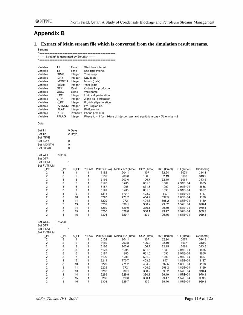
North Field, Qatar: A Study of Condensate Blockage and Petroleum Streams Management
Appendix B
1. Extract of Main stream file which is converted from the simulation result streams. Streamz 1* ==============================================* ----- StreamFile generated by Sen2Str ------* ==============================================
Variable T1 Time ; Start time intervalVariable T2 Time ; End time intervalVariable ITIME Integer ; Time stepVariable IDAY Integer ; Day (date)Variable IMONTH Integer ; Month (date)Variable IYEAR Integer ; Year (date)Variable OTP Real ; Ontime for productionVariable WELL String ; Well nameVariable I_PF Integer ; I grid cell perforationVariable J_PF Integer ; J grid cell perforationVariable K_PF Integer ; K grid cell perforationVariable PVTNUM Integer ; PVT region no.Variable IPLAT Integer ; Platform no.Variable PRES Pressure ; Phase pressureVariable PFLAG Integer ; Phase id = 1 for mixture of injection gas and equlibrium gas - Otherwise = 2
Data
Set T1 0 DaysSet T2 2 DaysSet ITIME 1Set IDAY 0Set IMONTH 0Set IYEAR 0
Set WELL P-0203 Set OTP 1Set IPLAT 1Set PVTNUM 1
I_PF J_PF K_PF PFLAG PRES (Psia) Moles N2 (lbmol) CO2 (lbmol) H2S (lbmol) C1 (lbmol) C2 (lbmol)2 3 1 1 5152 204.1 107 32.24 5074 314.32 3 2 1 5159 203.8 106.8 32.19 5067 313.92 3 3 1 5166 203.6 106.7 32.15 5061 313.52 3 5 1 5176 1205 631.3 1089 2.91E+04 18552 3 6 1 5187 1205 631.5 1090 2.91E+04 18562 3 7 1 5199 1206 631.8 1090 2.91E+04 18572 3 9 1 5211 770.7 403.9 697 1.86E+04 11872 3 10 1 5220 771.2 404.2 697.5 1.86E+04 11882 3 11 1 5229 772 404.6 698.2 1.86E+04 11892 3 13 1 5252 630.1 330.2 99.52 1.57E+04 970.42 3 14 1 5269 629.9 330.1 99.49 1.57E+04 970.12 3 15 1 5286 629.8 330.1 99.47 1.57E+04 969.92 3 16 1 5303 629.7 330 99.46 1.57E+04 969.8
Set WELL P-0208 Set OTP 1Set IPLAT 1Set PVTNUM 1
I_PF J_PF K_PF PFLAG PRES (Psia) Moles N2 (lbmol) CO2 (lbmol) H2S (lbmol) C1 (lbmol) C2 (lbmol)2 8 1 1 5152 204.1 107 32.24 5074 314.32 8 2 1 5159 203.8 106.8 32.19 5067 313.92 8 3 1 5166 203.6 106.7 32.15 5061 313.52 8 5 1 5176 1205 631.3 1089 2.91E+04 18552 8 6 1 5187 1205 631.5 1090 2.91E+04 18562 8 7 1 5199 1206 631.8 1090 2.91E+04 18572 8 9 1 5211 770.7 403.9 697 1.86E+04 11872 8 10 1 5220 771.2 404.2 697.5 1.86E+04 11882 8 11 1 5229 772 404.6 698.2 1.86E+04 11892 8 13 1 5252 630.1 330.2 99.52 1.57E+04 970.42 8 14 1 5269 629.9 330.1 99.49 1.57E+04 970.12 8 15 1 5286 629.8 330.1 99.47 1.57E+04 969.92 8 16 1 5303 629.7 330 99.46 1.57E+04 969.8
M.Sc. Thesis, IPT, 2004 Page 119 of 125
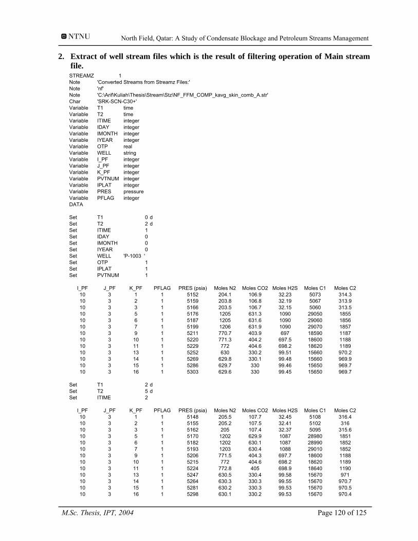
North Field, Qatar: A Study of Condensate Blockage and Petroleum Streams Management
2. Extract of well stream files which is the result of filtering operation of Main stream
file. STREAMZ 1Note 'Converted Streams from Streamz Files:'Note 'nf'Note 'C:\Arif\Kuliah\Thesis\Stream\Stz\NF_FFM_COMP_kavg_skin_comb_A.str'Char 'SRK-SCN-C30+'Variable T1 timeVariable T2 timeVariable ITIME integerVariable IDAY integerVariable IMONTH integerVariable IYEAR integerVariable OTP realVariable WELL stringVariable I_PF integerVariable J_PF integerVariable K_PF integerVariable PVTNUM integerVariable IPLAT integerVariable PRES pressureVariable PFLAG integerDATA
Set T1 0 dSet T2 2 dSet ITIME 1Set IDAY 0Set IMONTH 0Set IYEAR 0Set WELL 'P-1003 'Set OTP 1Set IPLAT 1Set PVTNUM 1
I_PF J_PF K_PF PFLAG PRES (psia) Moles N2 Moles CO2 Moles H2S Moles C1 Moles C210 3 1 1 5152 204.1 106.9 32.23 5073 314.310 3 2 1 5159 203.8 106.8 32.19 5067 313.910 3 3 1 5166 203.5 106.7 32.15 5060 313.510 3 5 1 5176 1205 631.3 1090 29050 185510 3 6 1 5187 1205 631.6 1090 29060 185610 3 7 1 5199 1206 631.9 1090 29070 185710 3 9 1 5211 770.7 403.9 697 18590 118710 3 10 1 5220 771.3 404.2 697.5 18600 118810 3 11 1 5229 772 404.6 698.2 18620 118910 3 13 1 5252 630 330.2 99.51 15660 970.210 3 14 1 5269 629.8 330.1 99.48 15660 969.910 3 15 1 5286 629.7 330 99.46 15650 969.710 3 16 1 5303 629.6 330 99.45 15650 969.7
Set T1 2 dSet T2 5 dSet ITIME 2
I_PF J_PF K_PF PFLAG PRES (psia) Moles N2 Moles CO2 Moles H2S Moles C1 Moles C210 3 1 1 5148 205.5 107.7 32.45 5108 316.410 3 2 1 5155 205.2 107.5 32.41 5102 31610 3 3 1 5162 205 107.4 32.37 5095 315.610 3 5 1 5170 1202 629.9 1087 28980 185110 3 6 1 5182 1202 630.1 1087 28990 185210 3 7 1 5193 1203 630.4 1088 29010 185210 3 9 1 5206 771.5 404.3 697.7 18600 118810 3 10 1 5215 772 404.6 698.2 18620 118910 3 11 1 5224 772.8 405 698.9 18640 119010 3 13 1 5247 630.5 330.4 99.58 15670 97110 3 14 1 5264 630.3 330.3 99.55 15670 970.710 3 15 1 5281 630.2 330.3 99.53 15670 970.510 3 16 1 5298 630.1 330.2 99.53 15670 970.4
M.Sc. Thesis, IPT, 2004 Page 120 of 125
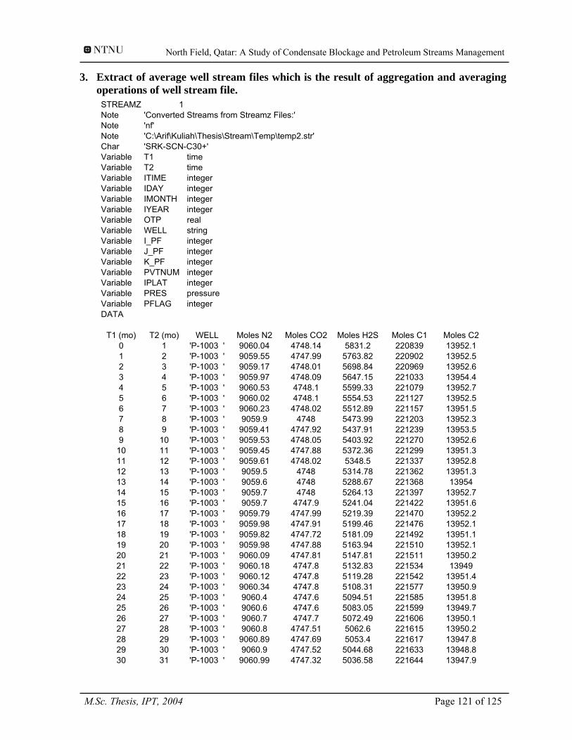
North Field, Qatar: A Study of Condensate Blockage and Petroleum Streams Management
3. Extract of average well stream files which is the result of aggregation and averaging
operations of well stream file. STREAMZ 1Note 'Converted Streams from Streamz Files:'Note 'nf'Note 'C:\Arif\Kuliah\Thesis\Stream\Temp\temp2.str'Char 'SRK-SCN-C30+'Variable T1 timeVariable T2 timeVariable ITIME integerVariable IDAY integerVariable IMONTH integerVariable IYEAR integerVariable OTP realVariable WELL stringVariable I_PF integerVariable J_PF integerVariable K_PF integerVariable PVTNUM integerVariable IPLAT integerVariable PRES pressureVariable PFLAG integerDATA
T1 (mo) T2 (mo) WELL Moles N2 Moles CO2 Moles H2S Moles C1 Moles C20 1 'P-1003 ' 9060.04 4748.14 5831.2 220839 13952.11 2 'P-1003 ' 9059.55 4747.99 5763.82 220902 13952.52 3 'P-1003 ' 9059.17 4748.01 5698.84 220969 13952.63 4 'P-1003 ' 9059.97 4748.09 5647.15 221033 13954.44 5 'P-1003 ' 9060.53 4748.1 5599.33 221079 13952.75 6 'P-1003 ' 9060.02 4748.1 5554.53 221127 13952.56 7 'P-1003 ' 9060.23 4748.02 5512.89 221157 13951.57 8 'P-1003 ' 9059.9 4748 5473.99 221203 13952.38 9 'P-1003 ' 9059.41 4747.92 5437.91 221239 13953.59 10 'P-1003 ' 9059.53 4748.05 5403.92 221270 13952.6
10 11 'P-1003 ' 9059.45 4747.88 5372.36 221299 13951.311 12 'P-1003 ' 9059.61 4748.02 5348.5 221337 13952.812 13 'P-1003 ' 9059.5 4748 5314.78 221362 13951.313 14 'P-1003 ' 9059.6 4748 5288.67 221368 1395414 15 'P-1003 ' 9059.7 4748 5264.13 221397 13952.715 16 'P-1003 ' 9059.7 4747.9 5241.04 221422 13951.616 17 'P-1003 ' 9059.79 4747.99 5219.39 221470 13952.217 18 'P-1003 ' 9059.98 4747.91 5199.46 221476 13952.118 19 'P-1003 ' 9059.82 4747.72 5181.09 221492 13951.119 20 'P-1003 ' 9059.98 4747.88 5163.94 221510 13952.120 21 'P-1003 ' 9060.09 4747.81 5147.81 221511 13950.221 22 'P-1003 ' 9060.18 4747.8 5132.83 221534 1394922 23 'P-1003 ' 9060.12 4747.8 5119.28 221542 13951.423 24 'P-1003 ' 9060.34 4747.8 5108.31 221577 13950.924 25 'P-1003 ' 9060.4 4747.6 5094.51 221585 13951.825 26 'P-1003 ' 9060.6 4747.6 5083.05 221599 13949.726 27 'P-1003 ' 9060.7 4747.7 5072.49 221606 13950.127 28 'P-1003 ' 9060.8 4747.51 5062.6 221615 13950.228 29 'P-1003 ' 9060.89 4747.69 5053.4 221617 13947.829 30 'P-1003 ' 9060.9 4747.52 5044.68 221633 13948.830 31 'P-1003 ' 9060.99 4747.32 5036.58 221644 13947.9
M.Sc. Thesis, IPT, 2004 Page 121 of 125
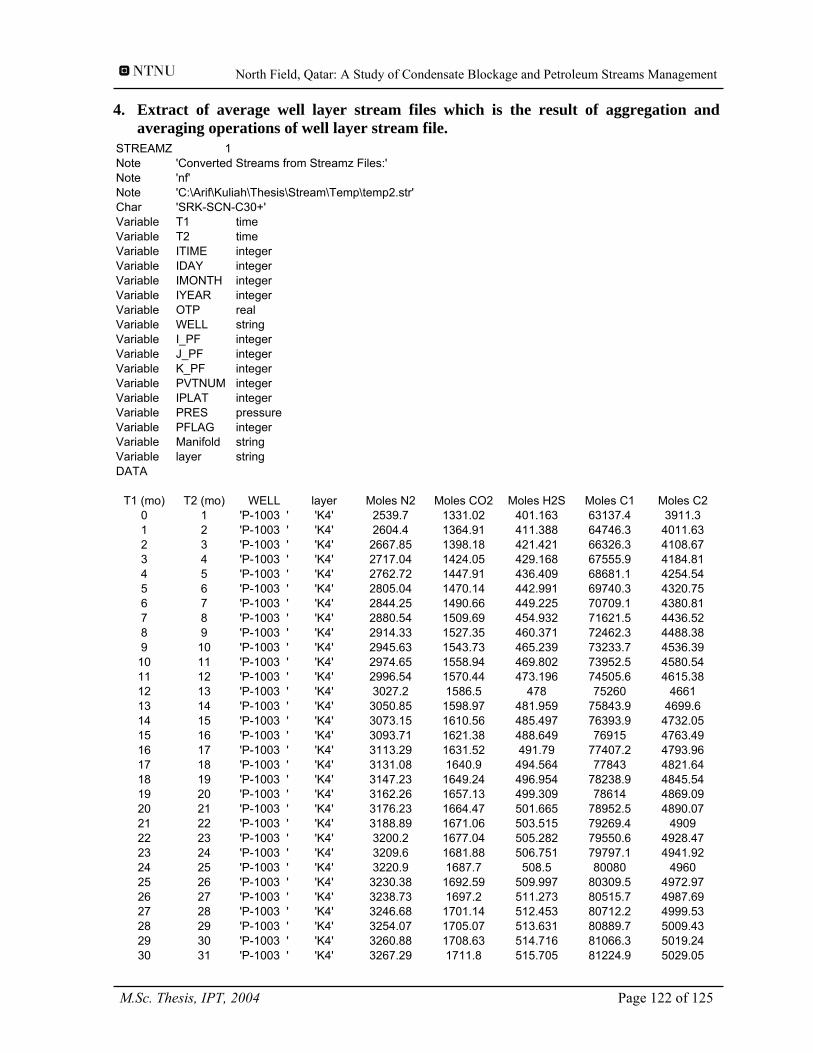
North Field, Qatar: A Study of Condensate Blockage and Petroleum Streams Management
4. Extract of average well layer stream files which is the result of aggregation and
averaging operations of well layer stream file. STREAMZ 1Note 'Converted Streams from Streamz Files:'Note 'nf'Note 'C:\Arif\Kuliah\Thesis\Stream\Temp\temp2.str'Char 'SRK-SCN-C30+'Variable T1 timeVariable T2 timeVariable ITIME integerVariable IDAY integerVariable IMONTH integerVariable IYEAR integerVariable OTP realVariable WELL stringVariable I_PF integerVariable J_PF integerVariable K_PF integerVariable PVTNUM integerVariable IPLAT integerVariable PRES pressureVariable PFLAG integerVariable Manifold stringVariable layer stringDATA
T1 (mo) T2 (mo) WELL layer Moles N2 Moles CO2 Moles H2S Moles C1 Moles C20 1 'P-1003 ' 'K4' 2539.7 1331.02 401.163 63137.4 3911.31 2 'P-1003 ' 'K4' 2604.4 1364.91 411.388 64746.3 4011.632 3 'P-1003 ' 'K4' 2667.85 1398.18 421.421 66326.3 4108.673 4 'P-1003 ' 'K4' 2717.04 1424.05 429.168 67555.9 4184.814 5 'P-1003 ' 'K4' 2762.72 1447.91 436.409 68681.1 4254.545 6 'P-1003 ' 'K4' 2805.04 1470.14 442.991 69740.3 4320.756 7 'P-1003 ' 'K4' 2844.25 1490.66 449.225 70709.1 4380.817 8 'P-1003 ' 'K4' 2880.54 1509.69 454.932 71621.5 4436.528 9 'P-1003 ' 'K4' 2914.33 1527.35 460.371 72462.3 4488.389 10 'P-1003 ' 'K4' 2945.63 1543.73 465.239 73233.7 4536.3910 11 'P-1003 ' 'K4' 2974.65 1558.94 469.802 73952.5 4580.5411 12 'P-1003 ' 'K4' 2996.54 1570.44 473.196 74505.6 4615.3812 13 'P-1003 ' 'K4' 3027.2 1586.5 478 75260 466113 14 'P-1003 ' 'K4' 3050.85 1598.97 481.959 75843.9 4699.614 15 'P-1003 ' 'K4' 3073.15 1610.56 485.497 76393.9 4732.0515 16 'P-1003 ' 'K4' 3093.71 1621.38 488.649 76915 4763.4916 17 'P-1003 ' 'K4' 3113.29 1631.52 491.79 77407.2 4793.9617 18 'P-1003 ' 'K4' 3131.08 1640.9 494.564 77843 4821.6418 19 'P-1003 ' 'K4' 3147.23 1649.24 496.954 78238.9 4845.5419 20 'P-1003 ' 'K4' 3162.26 1657.13 499.309 78614 4869.0920 21 'P-1003 ' 'K4' 3176.23 1664.47 501.665 78952.5 4890.0721 22 'P-1003 ' 'K4' 3188.89 1671.06 503.515 79269.4 490922 23 'P-1003 ' 'K4' 3200.2 1677.04 505.282 79550.6 4928.4723 24 'P-1003 ' 'K4' 3209.6 1681.88 506.751 79797.1 4941.9224 25 'P-1003 ' 'K4' 3220.9 1687.7 508.5 80080 496025 26 'P-1003 ' 'K4' 3230.38 1692.59 509.997 80309.5 4972.9726 27 'P-1003 ' 'K4' 3238.73 1697.2 511.273 80515.7 4987.6927 28 'P-1003 ' 'K4' 3246.68 1701.14 512.453 80712.2 4999.5328 29 'P-1003 ' 'K4' 3254.07 1705.07 513.631 80889.7 5009.4329 30 'P-1003 ' 'K4' 3260.88 1708.63 514.716 81066.3 5019.2430 31 'P-1003 ' 'K4' 3267.29 1711.8 515.705 81224.9 5029.05
M.Sc. Thesis, IPT, 2004 Page 122 of 125
North Field, Qatar: A Study of Condensate Blockage and Petroleum Streams Management
Appendix C
1. Spreadsheet calculation example for predicting the gas rate with excluding and including the capillary number effect
2. Spreadsheet calculation example for predicting the dry gas rate
M.Sc. Thesis, IPT, 2004 Page 123 of 125
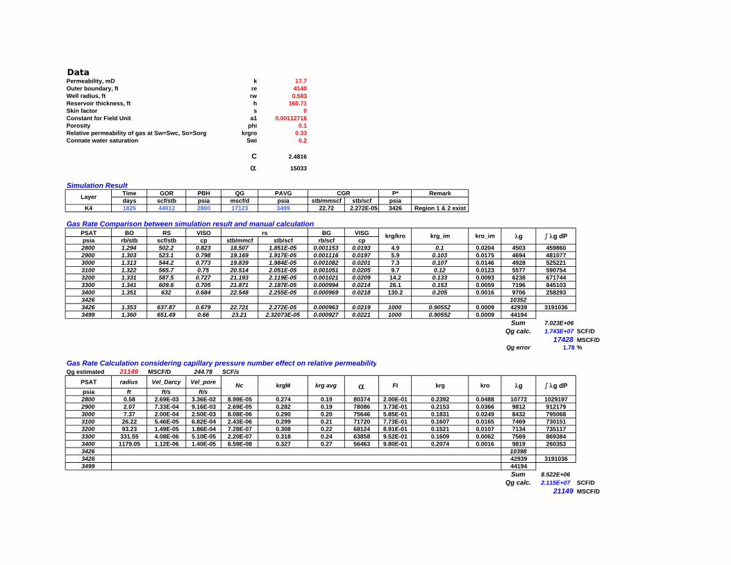
DataPermeability, mD k 17.7Outer boundary, ft re 4140Well radius, ft rw 0.583Reservoir thickness, ft h 160.71Skin factor s 0Constant for Field Unit a1 0.00112716Porosity phi 0.1Relative permeability of gas at Sw=Swc, So=Sorg krgro 0.33Connate water saturation Swi 0.2
C 2.4816
α 15033
Simulation ResultLayer Time GOR PBH QG PAVG CGR P* Remark
days scf/stb psia mscf/d psia stb/mmscf stb/scf psiaK4 1825 44012 2800 17123 3499 22.72 2.272E-05 3426 Region 1 & 2 exist
Gas Rate Comparison between simulation result and manual calculationPSAT BO RS VISO rs BG VISG krg/kro krg_im kro_im λg ∫ λg dPpsia rb/stb scf/stb cp stb/mmcf stb/scf rb/scf cp2800 1.294 502.2 0.823 18.507 1.851E-05 0.001153 0.0193 4.9 0.1 0.0204 4503 4598602900 1.303 523.1 0.798 19.169 1.917E-05 0.001116 0.0197 5.9 0.103 0.0175 4694 4810773000 1.313 544.2 0.773 19.839 1.984E-05 0.001082 0.0201 7.3 0.107 0.0146 4928 5252213100 1.322 565.7 0.75 20.514 2.051E-05 0.001051 0.0205 9.7 0.12 0.0123 5577 5907543200 1.331 587.5 0.727 21.193 2.119E-05 0.001021 0.0209 14.2 0.133 0.0093 6238 6717443300 1.341 609.6 0.705 21.871 2.187E-05 0.000994 0.0214 26.1 0.153 0.0059 7196 8451033400 1.351 632 0.684 22.548 2.255E-05 0.000969 0.0218 130.2 0.205 0.0016 9706 2582933426 103523426 1.353 637.87 0.679 22.721 2.272E-05 0.000963 0.0219 1000 0.90552 0.0009 42939 31910363499 1.360 651.49 0.66 23.21 2.32073E-05 0.000927 0.0221 1000 0.90552 0.0009 44194
Sum 7.023E+06Qg calc. 1.743E+07 SCF/D
17428 MSCF/DQg error 1.78 %
Gas Rate Calculation considering capillary pressure number effect on relative permeabilityQg estimated 21149 MSCF/D 244.78 SCF/s
PSAT radius Vel_Darcy Vel_pore Nc krgM krg avg α FI krg kro λg ∫ λg dPpsia ft ft/s ft/s2800 0.58 2.69E-03 3.36E-02 8.99E-05 0.274 0.19 80374 2.00E-01 0.2392 0.0488 10772 10291972900 2.07 7.33E-04 9.16E-03 2.69E-05 0.282 0.19 78086 3.73E-01 0.2153 0.0366 9812 9121793000 7.37 2.00E-04 2.50E-03 8.08E-06 0.290 0.20 75646 5.85E-01 0.1831 0.0249 8432 7950683100 26.22 5.46E-05 6.82E-04 2.43E-06 0.299 0.21 71720 7.73E-01 0.1607 0.0165 7469 7301513200 93.23 1.49E-05 1.86E-04 7.28E-07 0.308 0.22 68124 8.91E-01 0.1521 0.0107 7134 7351173300 331.55 4.08E-06 5.10E-05 2.20E-07 0.318 0.24 63858 9.52E-01 0.1609 0.0062 7569 8693843400 1179.05 1.12E-06 1.40E-05 6.59E-08 0.327 0.27 56463 9.80E-01 0.2074 0.0016 9819 2603533426 103983426 42939 31910363499 44194
Sum 8.522E+06Qg calc. 2.115E+07 SCF/D
21149 MSCF/D
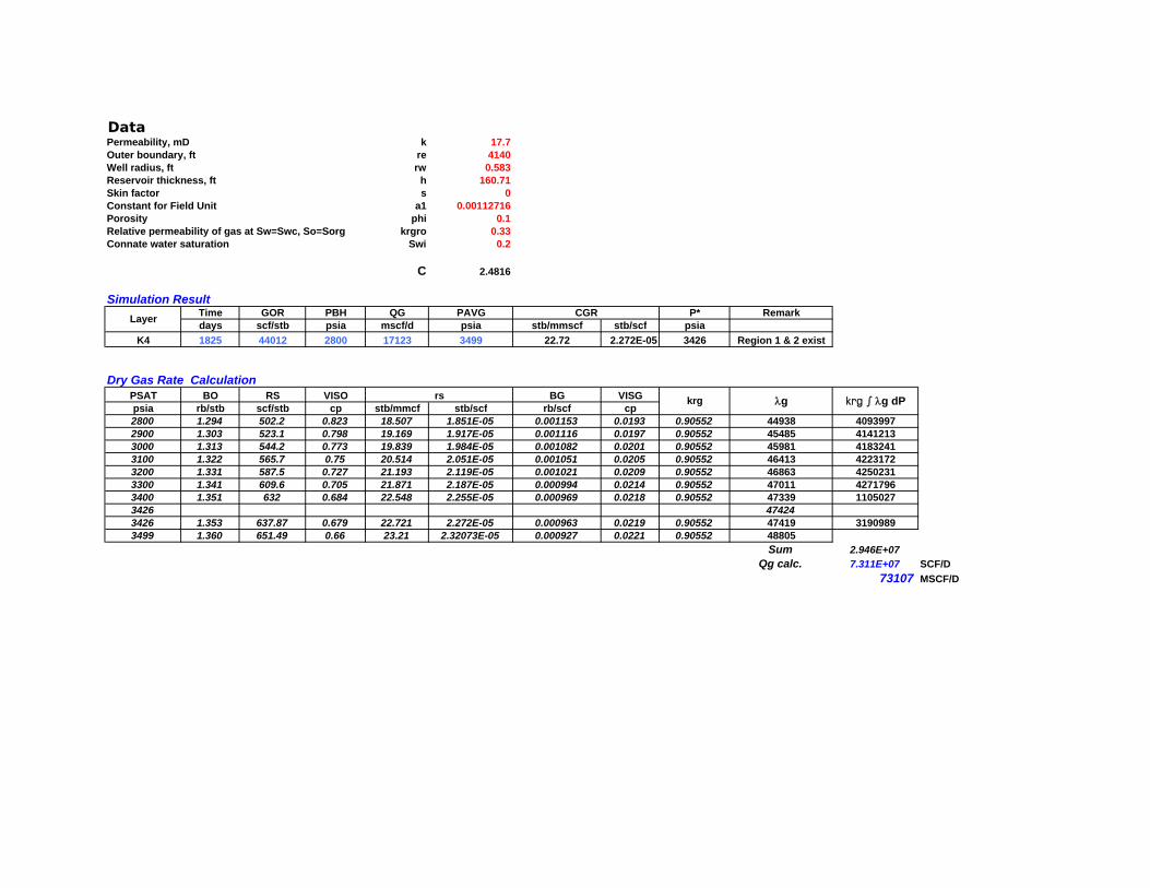
DataPermeability, mD k 17.7Outer boundary, ft re 4140Well radius, ft rw 0.583Reservoir thickness, ft h 160.71Skin factor s 0Constant for Field Unit a1 0.00112716Porosity phi 0.1Relative permeability of gas at Sw=Swc, So=Sorg krgro 0.33Connate water saturation Swi 0.2
C 2.4816
Simulation ResultLayer Time GOR PBH QG PAVG CGR P* Remark
days scf/stb psia mscf/d psia stb/mmscf stb/scf psiaK4 1825 44012 2800 17123 3499 22.72 2.272E-05 3426 Region 1 & 2 exist
Dry Gas Rate CalculationPSAT BO RS VISO rs BG VISG krg λg krg ∫ λg dPpsia rb/stb scf/stb cp stb/mmcf stb/scf rb/scf cp2800 1.294 502.2 0.823 18.507 1.851E-05 0.001153 0.0193 0.90552 44938 40939972900 1.303 523.1 0.798 19.169 1.917E-05 0.001116 0.0197 0.90552 45485 41412133000 1.313 544.2 0.773 19.839 1.984E-05 0.001082 0.0201 0.90552 45981 41832413100 1.322 565.7 0.75 20.514 2.051E-05 0.001051 0.0205 0.90552 46413 42231723200 1.331 587.5 0.727 21.193 2.119E-05 0.001021 0.0209 0.90552 46863 42502313300 1.341 609.6 0.705 21.871 2.187E-05 0.000994 0.0214 0.90552 47011 42717963400 1.351 632 0.684 22.548 2.255E-05 0.000969 0.0218 0.90552 47339 11050273426 474243426 1.353 637.87 0.679 22.721 2.272E-05 0.000963 0.0219 0.90552 47419 31909893499 1.360 651.49 0.66 23.21 2.32073E-05 0.000927 0.0221 0.90552 48805
Sum 2.946E+07Qg calc. 7.311E+07 SCF/D
73107 MSCF/D