normal tolerance interval procedures in the tolerance package · contributed research articles 200...

CONTRIBUTED RESEARCH ARTICLES 200

Normal Tolerance Interval Procedures inthe tolerance Packageby Derek S. Young

Abstract Statistical tolerance intervals are used for a broad range of applications, such as qualitycontrol, engineering design tests, environmental monitoring, and bioequivalence testing. toleranceis the only R package devoted to procedures for tolerance intervals and regions. Perhaps the mostcommonly-employed functions of the package involve normal tolerance intervals. A number of newprocedures for this setting have been included in recent versions of tolerance. In this paper, we discussand illustrate the functions that implement these normal tolerance interval procedures, one of whichis a new, novel type of operating characteristic curve.

Introduction and overview of the tolerance package

Statistical tolerance intervals of the form (1− α, P) provide bounds to capture at least a specifiedproportion P of the sampled population with a given confidence level 1− α. The quantity P is calledthe content of the tolerance interval and the confidence level 1− α reflects the sampling variability.There is an extensive literature on tolerance intervals with some of the earliest works being Wilks(1941, 1942) and Wald (1943). The texts by Guttman (1970) and Krishnamoorthy and Mathew (2009)are devoted to the theoretical development and application of tolerance intervals, while the text byHahn and Meeker (1991) discusses their application in the broader context of statistical intervals.

tolerance (Young, 2010) is a popular R package for constructing exact and approximate toleranceintervals and regions. Since its initial release in 2009, the package has grown to include toleranceinterval procedures for a large number of parametric distributions, nonparametric settings, andregression models. There are also tolerance region procedures for the multivariate normal andmultivariate regression settings. Procedures for more specific settings are also included, such asone-sided tolerance limits for the difference between two independent normal random variables(Hall, 1984) and fiducial tolerance intervals for the function of parameters from discrete distributions(Mathew and Young, 2013). The package also includes some graphical capabilities for visualizing thetolerance intervals (regions) by plotting the limits (regions) on histograms, scatterplots, or controlcharts of the data.

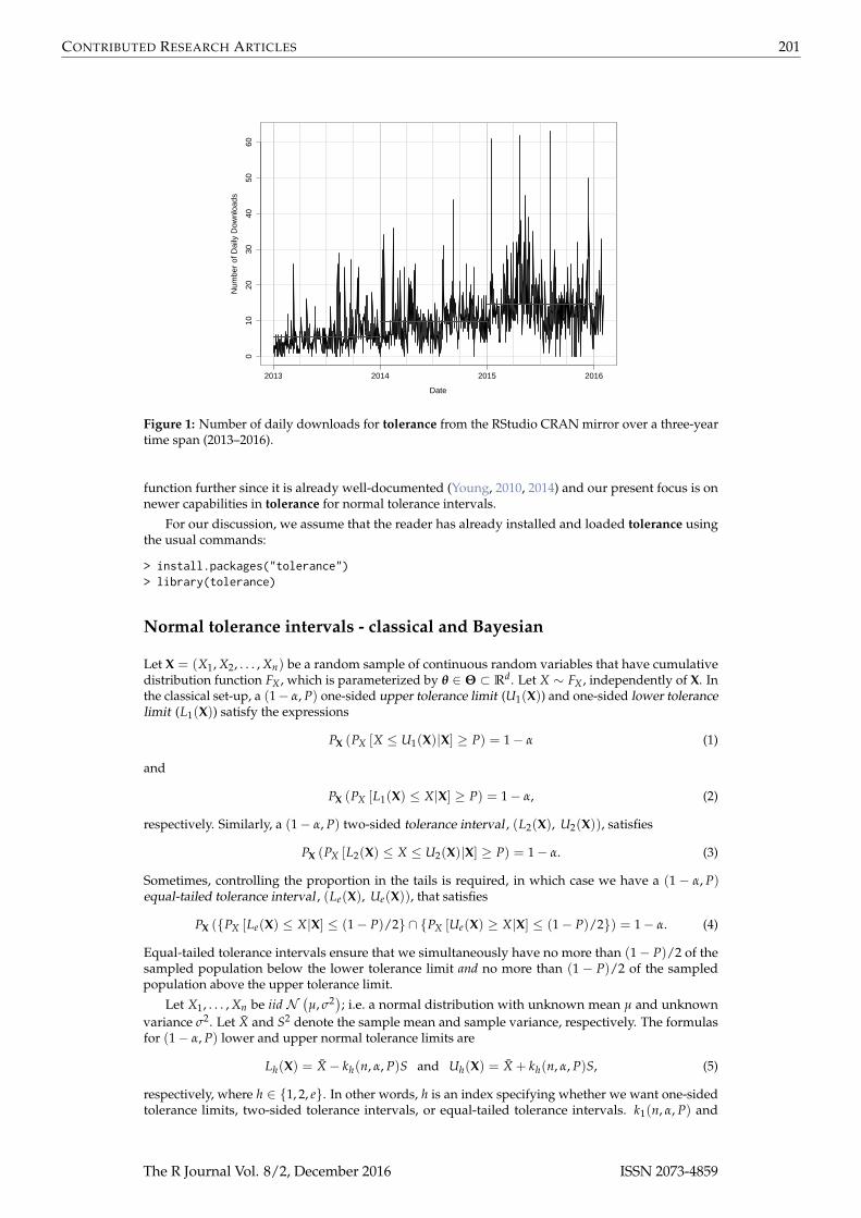
tolerance has been used for a broad range of applications, including cancer research (Heck et al.,2014), wildlife biology (Pasquaretta et al., 2012), assessing the performance of genetic algorithms(Van der Borght et al., 2014), ratio editing in surveys (Young and Mathew, 2015), air quality assessment(Hafner et al., 2013), and instrumentation testing (Burr and Gavron, 2010). General interest in tolerancecan be gauged by the cranlogs package (Csardi, 2015), which pulls download logs of the RStudio(RStudio Team, 2015) CRAN mirror. Figure 1 shows the daily number of downloads of tolerance fromthe beginning of 2013 to the beginning of 2016. There is clearly a general increasing trend over theyears as the average number of daily downloads per year is approximately 5, 10, and 15 in 2013, 2014,and 2015, respectively.

Capabilities of tolerance have been discussed in Young (2010, 2014). Even with those variedcapabilities, perhaps the most commonly used methods involve the normal distribution. Normaltolerance intervals are often required during design verification or process validation. The utility ofnormal tolerance intervals is further highlighted in documents published by the EPA (EnvironmentalProtection Agency, 2006), the IAEA (International Atomic Energy Agency, 2008), and standard 16269-6of the ISO (International Organization for Standardization, 2014). In this paper, we discuss newcapabilities in tolerance specifically involving normal tolerance intervals. This includes the calculationof exact and equal-tailed normal tolerance intervals, Bayesian normal tolerance intervals, toleranceintervals for fixed-effects ANOVA, and sample size determination strategies. We also introduce novelpseudo-operating characteristic (OC) curves that illustrate how the k-factor, sample size, confidencelevel, and content level each change relative to one another. Such curves can be useful for planningdesign tests.

As noted earlier, tolerance also includes a function for constructing multivariate normal tol-erance regions. The mvtol.region() function was included with the initial release of tolerance.mvtol.region() includes several Monte Carlo procedures developed in Krishnamoorthy and Mathew(1999) and Krishnamoorthy and Mondal (2006) for finding the k-factor of the multivariate normaltolerance region. The plottol() function can also be used to plot tolerance ellipses over bivariatenormal data and tolerance ellipsoids over trivariate normal data. The latter is accomplished usingplot3d() from the rgl package (Adler and Murdoch, 2014). We will not discuss the mvtol.region()

The R Journal Vol. 8/2, December 2016 ISSN 2073-4859

https://CRAN.R-project.org/package=tolerance

https://CRAN.R-project.org/package=cranlogs

https://CRAN.R-project.org/package=rgl


2013 2014 2015 2016

010

2030

4050

60

Date

Num

ber

of D

aily

Dow

nloa

ds

Figure 1: Number of daily downloads for tolerance from the RStudio CRAN mirror over a three-yeartime span (2013–2016).

function further since it is already well-documented (Young, 2010, 2014) and our present focus is onnewer capabilities in tolerance for normal tolerance intervals.

For our discussion, we assume that the reader has already installed and loaded tolerance usingthe usual commands:

> install.packages("tolerance")> library(tolerance)

Normal tolerance intervals - classical and Bayesian

Let X = (X1, X2, . . . , Xn) be a random sample of continuous random variables that have cumulativedistribution function FX , which is parameterized by θ ∈ Θ ⊂ Rd. Let X ∼ FX , independently of X. Inthe classical set-up, a (1− α, P) one-sided upper tolerance limit (U1(X)) and one-sided lower tolerancelimit (L1(X)) satisfy the expressions

PX (PX [X ≤ U1(X)|X] ≥ P) = 1− α (1)

and

PX (PX [L1(X) ≤ X|X] ≥ P) = 1− α, (2)

respectively. Similarly, a (1− α, P) two-sided tolerance interval , (L2(X), U2(X)), satisfies

PX (PX [L2(X) ≤ X ≤ U2(X)|X] ≥ P) = 1− α. (3)

Sometimes, controlling the proportion in the tails is required, in which case we have a (1− α, P)equal-tailed tolerance interval , (Le(X), Ue(X)), that satisfies

PX ({PX [Le(X) ≤ X|X] ≤ (1− P)/2} ∩ {PX [Ue(X) ≥ X|X] ≤ (1− P)/2}) = 1− α. (4)

Equal-tailed tolerance intervals ensure that we simultaneously have no more than (1− P)/2 of thesampled population below the lower tolerance limit and no more than (1− P)/2 of the sampledpopulation above the upper tolerance limit.

Let X1, . . . , Xn be iid N(µ, σ2); i.e. a normal distribution with unknown mean µ and unknown

variance σ2. Let X and S2 denote the sample mean and sample variance, respectively. The formulasfor (1− α, P) lower and upper normal tolerance limits are

Lh(X) = X− kh(n, α, P)S and Uh(X) = X + kh(n, α, P)S, (5)

respectively, where h ∈ {1, 2, e}. In other words, h is an index specifying whether we want one-sidedtolerance limits, two-sided tolerance intervals, or equal-tailed tolerance intervals. k1(n, α, P) and



k2(n, α, P) are the k-factors for these two settings. The k-factor ensures that we capture at least aproportion P of the sampled population with confidence level (1− α). k1(n, α, P) is calculated by

k1(n, α, P) =1√n

tn−1;1−α(√

nzP), (6)

where t f ;q(δ) is the qth quantile of a noncentral t-distribution with f degrees of freedom and noncen-trality parameter δ and zq is the qth quantile of the standard normal distribution. k2(n, α, P) is thesolution to the integral equation√

2nπ

∫ ∞

0P

(χ2

n−1 >(n− 1)χ2

1;P(z2)

k2(n, α, P)2

)e−

12 nz2

dz = 1− α, (7)

where χ2f is the chi-square random variable with f degrees of freedom and χ2

f ;q(δ) is the qth quantileof the noncentral chi-squared distribution with f degrees of freedom and noncentrality parameter δ.

Owen (1964) was the first to propose equal-tailed tolerance intervals for the normal distribution.Equal-tailed normal tolerance intervals still take the form of (5), but where the tolerance factorke(n, α, P) is found as the solution to the integral equation(

2n−1

2 Γ(

n− 12

))−1 ∫ ∞

(n−1)ϑ2n

nke (n,α,P)2

(2Φ(−ϑn +

ke(n, α, P)√

nz√n− 1

)− 1)

e−z/2zn−1

2 −1dz = 1− α, (8)

where ϑn =√

nz 1+P2

and Φ(·) denotes the standard normal cumulative distribution function. Ageneral discussion comparing the utility of two-sided tolerance intervals versus equal-tailed toleranceintervals is found in Jensen (2009).

The normtol.int() function in tolerance is able to calculate all of the one-sided tolerance limits,two-sided tolerance intervals, and equal-tailed tolerance intervals discussed above. In the past, chal-lenges with computing noncentral distributions necessitated the use of approximations for k1(n, α, P),k2(n, α, P), and ke(n, α, P). For the two-sided tolerance intervals, early versions of tolerance simplyused various approximations that appeared in the literature over the years for computing the k-factors.These are controlled through the method argument and their specific formulas are outlined in Young(2010), which utilized tolerance version 0.2.2. Since then, the exact k-factor in (7) and the exact equal-tailed k-factor in (8) have been included. These are implemented by setting method = "EXACT" andmethod = "OCT", respectively. Both of these methods use adaptive quadrature via the integrate()function as well as box-constrained optimization via the optim() function. The original approximationmethods are still available primarily to retain all functionality of previous versions of tolerance.

The dataset that we will use to illustrate most of the procedures in our discussion is a qualitycontrol dataset from Krishnamoorthy and Mathew (2009). The data are from a machine that fillsplastic containers with a liter of milk. At the end of a particular shift, a sample of n = 20 containerswas selected and the actual amount of milk in each container was measured using a highly-accuratemethod. These measurements are as follows:

> milk <- c(0.968, 0.982, 1.030, 1.003, 1.046,+ 1.020, 0.997, 1.010, 1.027, 1.010,+ 0.973, 1.000, 1.044, 0.995, 1.020,+ 0.993, 0.984, 0.981, 0.997, 0.992)

A quick check of normality with the Shapiro-Wilk test confirms that this is an appropriate assumption:

> shapiro.test(milk)

Shapiro-Wilk normality test

data: milkW = 0.96364, p-value = 0.6188

For the milk data, the (0.95, 0.90) one-sided tolerance limits, two-sided tolerance interval, andequal-tailed tolerance interval are found as follows:

> normtol.int(x = milk, alpha = 0.05, P = 0.90, side = 1)alpha P x.bar 1-sided.lower 1-sided.upper

1 0.05 0.9 1.0036 0.9610333 1.046167

> normtol.int(x = milk, alpha = 0.05, P = 0.90, side = 2, method = "EXACT", m = 50)alpha P x.bar 2-sided.lower 2-sided.upper



1 0.05 0.9 1.0036 0.9523519 1.054848

> normtol.int(x = milk, alpha = 0.05, P = 0.90, side = 2, method = "OCT", m = 50)alpha P x.bar 2-sided.lower 2-sided.upper

1 0.05 0.9 1.0036 0.9471414 1.060059

Note that the equal-tailed tolerance interval is wider than the corresponding two-sided toleranceinterval due to the more stringent requirement of controlling the proportions in the tails. For thetwo-sided tolerance intervals, the additional argument m is used to control the number of subintervalsto use for performing the numerical integration via integrate(). While not illustrated above, thereis an additional argument that can be used if one wishes to construct log-normal tolerance intervals.The argument log.norm is a logical argument set to FALSE by default. If set to TRUE, log-normaltolerance intervals are calculated using the fact that if X is log-normally distributed, then Y = log(X)is normally distributed. Thus, the normtol.int() function simply takes the logarithm of the data inthe x argument, constructs the desired normal tolerance limits, and then takes the anti-log of thoselimits.

Users of normal tolerance intervals are often interested in summarizing a variety of possiblek-factors for given sample sizes n, confidence levels 1− α, and content level P. The K.table functionallows the user to specify a vector of possible values for each of these three quantities. A list isthen returned whose elements are summarized according to the by argument. For example, supposewe are interested in the k1(n, α, P) values for all combinations of n ∈ {10, 20}, α ∈ {0.01, 0.05}, andP ∈ {0.95, 0.99}. Moreover, we would like to summarize the list by the levels of P. This is accomplishedas follows:

> K.table(n = c(10, 20), alpha = c(0.01, 0.05), P = c(0.95, 0.99),+ side = 1, by.arg = "P")$`0.95`

10 200.99 3.738315 2.8078660.95 2.910963 2.396002

$`0.99`10 20

0.99 5.073725 3.8315580.95 3.981118 3.295157

For example, the first entry of the first matrix is the k-factor for a one-sided (0.99, 0.95) tolerance limitwhen n = 10. One can also set side = 2, which requires the user to specify the method argument; e.g."EXACT" for values of k2(n, α, P) or "OCT" for values of ke(n, α, P). The by.arg argument can also be setto "alpha" or "n" depending on which quantity you want to represent the elements of the outputtedlist.

Bayesian tolerance intervals were first presented in Aitchison (1964). For the Bayesian set-up, let xbe a vector of realizations of X, L(θ|x) be the likelihood function, π(θ) be a prior distribution for θ,and p(θ|x) be the posterior distribution of θ given by

p(θ|x) = L(θ|x)π(θ)∫Θ L(θ|x)π(θ)dθ

. (9)

Then, (1− α, P) Bayesian one-sided upper and lower tolerance limits satisfy

PΘ (PX [X ≤ U1(θ)|θ] ≥ P|X) = 1− α (10)

and

PΘ (PX [L1(θ) ≤ X|θ] ≥ P|X) = 1− α, (11)

respectively, a (1− α, P) Bayesian two-sided tolerance interval satisfies

PΘ (PX [L2(θ) ≤ X ≤ U2(θ)|θ] ≥ P|X) = 1− α, (12)

and a (1− α, P) Bayesian equal-tailed tolerance interval satisfies

PΘ ({PX [Le(θ) ≤ X|θ] ≤ (1− P)/2} ∩ {PX [Ue(θ) ≥ X|θ] ≤ (1− P)/2}|X) = 1− α. (13)

Notice that the Bayesian set-up is calculated with respect to the probability measure PΘ while theclassical set-up is calculated with respect to the distribution of the random sample X. We refer thereader to the texts by Guttman (1970) and Krishnamoorthy and Mathew (2009) for more details on



both classical and Bayesian tolerance intervals.

The parameters µ and σ2 are still assumed unknown. We use the conjugate priors π(µ|σ2) andπ(σ2), which are

µ|σ2 ∼ N(

µ0, σ2/n0

)and σ2 ∼ Scale-inv-χ2

(m0, σ2

0

), (14)

respectively, where Scale-inv-χ2 (ν, τ2) is the scaled inverse chi-squared distribution with ν de-grees of freedom and scaling parameter τ2. Thus, the joint prior density of

(µ, σ2) is π

(µ, σ2) =

π(µ|σ2)π

(σ2). The four hyperparameters for this prior structure are µ0 ∈ R, σ2

0 > 0, m0 > 0, n0 > 0.m0 and n0 are not prior sample size quantities, but are tunable quantities to reflect the prior precisionrelative to the sample size. The joint posterior distribution is then

p(

µ, σ2|x)= p

(µ|σ2

)p(

σ2)

, (15)

where p(µ|σ2) and p

(σ2) are the distributions

µ|σ2 ∼ N(

¯x,σ2

n0 + n

)and σ2 ∼ Scale-inv-χ2

(m0 + n− 1, q2

), (16)

respectively, such that

¯x =n0µ0 + nx

n0 + nand q2 = (m0 + n− 1)−1

[m0σ2

0 + (n− 1)s2 +n0n

n0 + n(x− µ0)

2]

. (17)

Note that the formulas in the Bayesian set-up are written such that they are conditioned on realizationsof the observed data; i.e. X = x. Furthermore, they are written in terms of the sample estimates of themean (x) and variance (s2). Additional details on the above can be found, for example, in Chapter 3 ofGelman et al. (2013).

Similar to the classical setting, (1− α, P) Bayesian lower and upper normal tolerance limits are,respectively,

Lh

(x, s2

)= ¯x− kh (n, n0, m0, α, P) q and Uh

(x, s2

)= ¯x + kh (n, n0, m0, α, P) q, (18)

where, again, h is used as an index for one-sided limits, a two-sided interval, or an equal-tailed interval.Note that these limits are expressed in terms the maximum likelihood estimates of µ and σ2, whichoccur through how ¯x and q are defined. Thus, the one-sided k-factor is calculated by

k1 (n, n0, m0, α, P) =1√

n0 + ntm0+n−1;1−α

(√n0 + nzP

), (19)

the two-sided k-factor k2 (n, n0, m0, α, P) is calculated by finding the solution to√2(n0 + n)

π

∫ ∞

0P

(χ2

m0+n−1 >(m0 + n− 1) χ2

1;P(z2)

k2 (n, n0, m0, α, P)2

)e−

12 (n0+n)z2

dz = 1− α, (20)

and the equal-tailed k-factor ke (n, n0, m0, α, P) is calculated by finding the solution to

2−(

m0+n−12

)Γ(

m0+n−12

) ∫ ∞(m0+n−1)ϑ2

n0+n(n0+n)ke (n,n0,m0,α,P)2

(2Φ(−ϑn0+n +

ke(n, n0, m0, α, P)√

n0 + nz√m0 + n− 1

)− 1)

× e−z/2zm0+n−1

2 −1dz = 1− α.

(21)

Finally, if one considers the non-informative prior distribution

π(µ, σ2) ∝ σ−2, (22)

the solutions for the one-sided Bayesian normal tolerance limits and two-sided Bayesian normaltolerance intervals are the same as for the classical setting given in Equations (5)–(8); see Chapter 11 ofKrishnamoorthy and Mathew (2009) for the details.

The bayesnormtol.int() function for computing Bayesian normal tolerance intervals is new asof tolerance version 1.1.1. It was composed to closely mirror the normtol.int() function. For themilk data, suppose we use the conjugate prior structure in (14). Assuming we have some historicalknowledge about the milk filling process, the following hyperparameter values are used: µ0 = 1.000,σ2 = 0.001, and m0 = n0 = 20. Then, the Bayesian (0.95, 0.90) one-sided tolerance limits, two-sided



tolerance interval, and equal-tailed tolerance interval are found as follows:

> bayesnormtol.int(x = milk, alpha = 0.05, P = 0.90, side = 1,+ hyper.par = list(mu.0 = 1.000, sig2.0 = 0.001,+ m.0 = 20, n.0 = 20))alpha P 1-sided.lower 1-sided.upper

1 0.05 0.9 0.9551936 1.048406

> bayesnormtol.int(x = milk, alpha = 0.05, P = 0.90, side = 2, method = "EXACT",+ m = 50, hyper.par = list(mu.0 = 1.000, sig2.0 = 0.001,+ m.0 = 20, n.0 = 20))alpha P 2-sided.lower 2-sided.upper

1 0.05 0.9 0.9453603 1.05824

> bayesnormtol.int(x = milk, alpha = 0.05, P = 0.90, side = 2, method = "OCT",+ m = 50, hyper.par = list(mu.0 = 1.000, sig2.0 = 0.001,+ m.0 = 20, n.0 = 20))alpha P 2-sided.lower 2-sided.upper

1 0.05 0.9 0.9407625 1.062838

The bayesnormtol.int() function has the arguments x, alpha, P, side, method, and m just as in thenormtol.int(). However, here we also have hyper.par, which is a list with elements for the fourhyperparameters. The output is structured identically to the output obtained using normtol.int(),which allows for easy comparison between the classical and Bayesian results.

Fixed-effects ANOVA tolerance intervals

The approach for classical normal tolerance intervals can be easily extended for the balanced fixed-effects ANOVA model

Yij...kl = θ + αi + β j + . . . + γk + εij...kl , (23)

where θ is the grand mean, αi, β j, . . . , γk are the factor effects each subject to the constraint that thesummation of the effects over the respective index is equal to 0, εij,...kl are iid N

(0, σ2) error terms,

and the indices are i = 1, . . . , a, j = 1, . . . , b, . . ., k = 1, . . . , c, and l = 1, . . . , n. The approach discussedbelow is for the classical setting. Currently, the tolerance package does not have a function forcalculating Bayesian ANOVA tolerance intervals.

Let Y ∈ Rab···cn be a vector of all of the measured responses in (23), which are iid N(0, σ2). The

formulas for the tolerance limits in the fixed-effects ANOVA setting are:

Li;h(Y) = Yi·...·· − kh (ni, f , α, P)√

MSE and Ui;h(Y) = Yi·...·· + kh (ni, f , α, P)√

MSE

Lj;h(Y) = Y·j...·· − kh

(nj, f , α, P

)√MSE and Uj;h(Y) = Y·j...·· + kh

(nj, f , α, P

)√MSE

......

Lk;h(Y) = Y··...k· − kh (nk, f , α, P)√

MSE and Uk;h(Y) = Y··...k· + kh (nk, f , α, P)√

MSE(24)

Conceptually, the formulas in (24) are similar to those in (5). We take a point estimate of the meanat each factor level (i.e. the quantities Yi·...··, Y·j...··, . . . , Y··...k·) and then add or subtract the k-factortimes the standard deviation. The standard deviation is now estimated by the root mean square error,√

MSE.

The k-factor in (24), again, has the subscript h to indicate an index for one-sided limits, a two-sidedinterval, or an equal-tailed interval. However, the formulas are modified for the ANOVA setting. Informulas (6)–(8), the quantity (n− 1) reflects the degrees of freedom when estimating the samplevariance S2. In the ANOVA setting, this is replaced by the degrees of freedom due to the error; i.e. thedegrees of freedom associated with the MSE. Thus, we replace each occurrence of (n− 1) in (6)–(8)with f , the error degrees of freedom. Moreover, all occurrences of the sample size n are replaced withthe number of observations at each factor level; i.e. ni, nj, . . . , nk. Note that the tolerance intervalspresented are only accurate for balanced (or nearly-balanced) ANOVA settings.

We analyze the well-known dataset that resulted from an experimental design regarding the effectsof wool type and the amount of tension applied to a loom of yarn on the number of warp breaks thatoccur on that loom of yarn (Tippett, 1950). The first factor is wool type, which has two levels: A or B.



The second factor is tension level, which has three levels: low (L), medium (M), or high (H). The sixtreatments (i.e. factor level combinations) are randomly assigned to one of 54 looms of yarn. Thus, wehave n = 9 replicates per treatment. Suppose we want to construct (0.85, 0.90) equal-tailed toleranceintervals for each factor level’s mean. Below is how we would do this in the tolerance package:

> lm.out <- lm(breaks ~ wool + tension, data = warpbreaks)> out <- anovatol.int(lm.out, data = warpbreaks, alpha = 0.10,+ P = 0.85, side = 2, method = "OCT")These are 90%/85% 2-sided tolerance intervals.> out$wool

mean n k 2-sided.lower 2-sided.upperA 31.03704 27 1.886857 9.117165 52.95691B 25.25926 27 1.886857 3.339387 47.17913

$tensionmean n k 2-sided.lower 2-sided.upper

L 36.38889 18 1.948567 13.7521219 59.02566M 26.38889 18 1.948567 3.7521219 49.02566H 21.66667 18 1.948567 -0.9701003 44.30343

In the anovatol.int() function, we have similar arguments as in the normtol.int() function, exceptnow we input an object of class "lm" and we also tell the function the name of the original datasetusing the data argument. The output is a list summarizing the tolerance interval results for each factorlevel. For example, the (0.90, 0.85) equal-tailed tolerance interval for the medium tension applied tothe yarn is about (3.75, 49.03).

010

2030

4050

6070

wool

breaks

A B

90% / 85% Tolerance Intervals for wool

010

2030

4050

6070

tension

breaks

L M H

90% / 85% Tolerance Intervals for tension

Figure 2: Plot of the (0.85, 0.90) equal-tailed tolerance intervals for the yarn strength data.

We can also produce a figure of the above output by using the plottol() function as follows:

> plottol(out, x = warpbreaks)

The above produces the plot in Figure 2. This figure has a separate panel for each factor. The y-axis isthe response and the x-axis is the levels of the respective factor. The solid black point is the factor levelmean and the red lines extend to the lower and upper tolerance limits calculated earlier. Such a figureprovides a relative comparison of the tolerance intervals for each factor level.

Sample size determination strategies

As noted in Faulkenberry and Weeks (1968), an important question for statistical practitioners is "Whatsample size should be used to determine the tolerance limits?" Those same authors addressed thisproblem by developing an approach to ensure that the calculated tolerance intervals are "close" tothe quantiles that result in a content level at least as large as P. Their solution was developed for



sample size determination of one-sided tolerance limits and two-sided tolerance intervals, but it is notapplicable to equal-tailed tolerance intervals. In order to briefly present their approach, let Cµ,σ(X)denote any of the three inner probabilities in Equations (1)–(3) or any of the three analogous innerprobabilities for the Bayesian set-up in Equations (10)–(12). To ensure the "goodness" of the tolerancelimits (interval), one must choose an arbitrary P′ > P and small δ > 0 to determine a sample size n∗

such that

PX{

Cµ,σ(X) ≥ P′}≥ δ (25)

or

Pθ

{Cµ,σ(X) ≥ P′

}≥ δ (26)

for the classical or Bayesian setting, respectively.

The norm.ss function for sample size determination of normal tolerance limits (intervals) is newas of tolerance version 1.1.1. The function finds the minimum sample size n∗ for the approachdue to Faulkenberry and Weeks (1968) discussed above. For our example, suppose the qualityengineer overseeing the milk-filling process wants to submit a future sample of liters of milk tothe highly-accurate measurement method. Per the company’s guidelines, the engineer needs toknow the minimum sample size to construct a (0.95, 0.90) two-sided tolerance interval such thatPX{

Cµ,σ(X) ≥ 0.97}≥ 0.10. This is calculated as follows:

> norm.ss(alpha = 0.05, P = 0.90, delta = 0.10, P.prime = 0.97,+ side = 2, m = 50, method = "FW")alpha P delta P.prime n

1 0.05 0.9 0.1 0.97 60

Thus, the engineer would need a minimum sample size of n∗ = 60 to ensure that there is only a smallprobability δ = 0.10 that the (0.95, 0.90) tolerance interval will have a content exceeding P = 0.90 by(P′ − P) = 0.07.

In the norm.ss() function, the argument method is set to "FW". There are two additional samplesize determination strategies that can be calculated, which are controlled through the method argument.Both of these strategies assume there is some historical data and specification limits for the processat-hand. We briefly illustrate these strategies below and refer the reader to Young et al. (2016) forfurther details.

The first alternative strategy is a simple “back-of-the-envelope” calculation. We consider theproblem of designing a study to demonstrate that a process or product falls within the specificationlimits (SL, SU). We are interested in the minimum sample size necessary such that a (1− α, P) one-sided lower tolerance limit exceeds SL, a (1− α, P) one-sided upper tolerance limit falls below SU , ora (1− α, P) two-sided tolerance interval is contained within (SL, SU). In other words, this requiresfinding the minimum sample size n∗ such that

SL < µ− k1(n, α, P)σ; (27)

SU > µ + k1(n, α, P)σ; or (28)

µ± ke(n, α, P)σ ⊂ (SL, SU), (29)

for one-sided upper tolerance limits, one-sided lower tolerance limits, or equal-tailed toleranceintervals, respectively. As emphasized in Young et al. (2016), this approach is intended simply forplanning purposes and it does not guarantee any specific bounds relative to the nominal coverageprobability. Note that (29) is for an equal-tailed tolerance interval since we posit values for µ and σand, thus, the resulting tolerance interval would be built around a (hypothetically) true center of thenormal population.

For our example, suppose that the quality engineer is overseeing the launch of a new process forfilling the one-liter containers of milk, which is intended to be more accurate than the previous process.The company set specification limits at (0.990, 1.010). For determining the minimum sample sizenecessary to construct a (0.95, 0.90) two-sided tolerance interval that is within the specification limits,the engineer assumes the mean and variance from the data of the original process. This calculationcan then be done as follows:

> norm.ss(alpha = 0.05, P = 0.90, side = 2, spec = c(0.990, 1.010),+ method = "DIR", hyper.par = list(mu.0 = 1.004, sig2.0 = 0.001))alpha P delta P.prime n

1 0.05 0.9 5

Thus, the minimum sample size is n∗ = 5. This calculation was done by setting method = "DIR",entering the specification limits in the spec argument, and entering the assumed µ and σ2 in the



argument hyper.par.

The second alternative strategy presented in Young et al. (2016) is a method for providing data-dependent values of the precision quantities P′ and δ in the approach due to Faulkenberry and Weeks(1968). The approach assumes there is information on historical data, a set of current data, andspecification limits that can be used for calculating values of P′ and δ. The approach is intended to beused when there is no practical guidance for setting these values other than using “rule-of-thumb”quantities suggested in Faulkenberry and Weeks (1968).

For the milk filling process, suppose the engineer has historical measurements, which have acombined mean 0.994 liters and variance 0.002. Suppose the specification limits on the original processare (0.900, 1.100) and that the engineer needs a minimum sample size to construct a (0.95, 0.90) two-sided tolerance interval to show that the process meets the specification limits. However, the engineeris unsure about levels to choose for δ and P′. We can use the norm.ss() function as follows:

> norm.ss(x = milk, alpha = 0.05, P = 0.90, side = 2, spec = c(0.900, 1.100),+ method = "YGZO", hyper.par = list(mu.0 = 0.994, sig2.0 = 0.002))alpha P delta P.prime n

1 0.05 0.9 0.1807489 0.9733307 42

Thus, the engineer would need a minimum sample size of n∗ = 42 to ensure that there is only aprobability of about δ = 0.181 that the (0.95, 0.90) tolerance interval will have a content exceedingP = 0.90 by about (P′ − P) = 0.073.

OC curves involving k-factors

Sometimes, engineers and industrial statisticians are interested in understanding how the confidencelevel or content level changes as a function of n for a given level of the k-factor. If one has normallydistributed data that they intend to demonstrate meets certain specification limits, then it is importantto understand the type of values for 1− α and P that one can reasonably expect to use. In this section,we present OC curves for such planning purposes.

The first type of OC curve is used when one specifies a range of values of the sample size n and atarget value of the k-factor. Then, one can either specify a set of 1− α values and solve for P or one canspecify a set of P values and solve for 1− α. The values of n are plotted on the x-axis and the valuebeing solved for – either P or 1− α – is plotted on the y-axis. The different OC curves pertain to theset of specified values – either 1− α or P. Since too many curves can become cumbersome, we haveplaced an upper limit of 10 curves that can be overlaid on a given plot. Also, the colors used for thecurves were chosen using a colorblind-friendly palette that was established by Okabe and Ito (2002).

Suppose a company is designing a product and the engineer needs to collect enough data so thatthe resulting two-sided tolerance interval will have a k-factor of 4. Content levels under considerationare P ∈ {0.90, 0.95, 0.99} while the possible number of samples that can be used for the test aren = 10, 11, . . . , 20. In order to determine the resulting confidence levels that can be obtained underthese conditions, the engineer can construct an OC curve for 1− α using the following code:

norm.OC(k = 4, alpha = NULL, P = c(0.90, 0.95, 0.99), n = 10:20,side = 2, method = "EXACT", m = 25)

The resulting plot is given in Figure 3. For example, if the engineer chooses n = 15, then they canconstruct a two-sided tolerance interval with k = 4 and content level of P = 0.99 with confidence levelnear 0.96. However, if the engineer wishes to decrease the content of the tolerance interval to P = 0.95or P = 0.90, then a confidence level very near 1 can be achieved.

In the norm.OC() function, the arguments of side, method, and m are, again, passed down to theunderlying K.factor() function. In order to generate Figure 3, we need to specify a single value for k(i.e. the k-factor) and at least one value for P. Since we are constructing curves where the sample size ison the x-axis, we need at least two values for n. Note that alpha must be left at its default NULL value.

Suppose now that the same engineer considers confidence levels of 1− α ∈ {0.90, 0.95, 0.99} withthe same values of k and n from before. In order to determine the resulting content levels that can beobtained under these conditions, the engineer can construct an OC curve for P using the followingcode:

norm.OC(k = 4, alpha = c(0.01, 0.05, 0.10), P = NULL, n = 10:20,side = 2, method = "EXACT", m = 25)

The resulting plot is given in Figure 4. For example, if the engineer chooses n = 12, then they canconstruct a two-sided tolerance interval with k = 4 and confidence level of 1− α = 0.99 that capturesabout 95% of the sampled population. However, if the engineer wishes to decrease the confidence level



10 12 14 16 18 20

0.92

0.94

0.96

0.98

1.00

Normal Tolerance Interval OC Curve for 1- α (k=4)

n

1-α

P0.9000.9500.990

Figure 3: OC curves for 1 − α given the set of content levels P ∈ {0.90, 0.95, 0.99}, sample sizesn = 10, 11, . . . , 20, and a two-sided k-factor of 4.

10 12 14 16 18 20

0.93

0.95

0.97

0.99

Normal Tolerance Interval OC Curve for P (k=4)

n

P

1-α0.9000.9500.990

Figure 4: OC curves for P given the set of confidence levels 1− α ∈ {0.90, 0.95, 0.99}, sample sizesn = 10, 11, . . . , 20, and a two-sided k-factor of 4.

of the tolerance interval to 1− α = 0.95 or 1− α = 0.90, then a tolerance interval that captures about99% of the sampled population can be achieved. Note that the code using the norm.OC() function issimilar to the previous example, except that now we specify at least one value for alpha and leave Pmust at its default NULL value.

Finally, the norm.OC() function can also be used to construct an OC-curve where the k-factor iscalculated for specified values of n, 1− α, and P. The different curves will be for each combination ofthe specified 1− α and P levels. For our example, suppose the engineer is interested in the k-factorsfor two-sided tolerance intervals for the set of confidence levels 1− α ∈ {0.90, 0.95, 0.99}, the set ofcontent levels P ∈ {0.90, 0.95, 0.99}, and sample sizes n = 10, 11, . . . , 20. Then, we can specify therespective arguments in the norm.OC() function while leaving the k argument at its default NULL value:

norm.OC(k = NULL, P = c(0.90, 0.95, 0.99), alpha=c(0.01, 0.05, 0.10),n = 10:20, side = 2, method = "EXACT", m = 25)

The resulting plot is given in Figure 5. This OC-curve allows the user to assess the width of thetolerance interval as n changes for the given (1− α, P) tolerance levels.

Summary

tolerance is the only R package devoted to the calculation of tolerance intervals and regions. Since itsearlier versions (Young, 2010), there have been many updates to the package that include additionalparametric tolerance interval procedures, improved nonparametric tolerance interval procedures, andsome multivariate tolerance region procedures.



10 12 14 16 18 20

01

23

45

Normal Tolerance Interval OC Curve for k and n

n

k

(1-α,P)

(0.990,0.900)(0.950,0.900)(0.900,0.900)(0.990,0.950)(0.950,0.950)(0.900,0.950)(0.990,0.990)(0.950,0.990)(0.900,0.990)

Figure 5: OC curves for the k-factor when given the set of confidence levels 1− α ∈ {0.90, 0.95, 0.99},the set of content levels P ∈ {0.90, 0.95, 0.99}, and sample sizes n = 10, 11, . . . , 20.

In this paper, we focused on the varied capabilities of tolerance pertaining to tolerance intervalsfor the normal distribution. Many of these procedures have been added to the package since thediscussion presented in Young (2010). We discussed the calculation of one-sided normal tolerancelimits, exact and equal-tailed normal tolerance intervals, Bayesian normal tolerance intervals, toleranceintervals for fixed-effects ANOVA, and sample size determination strategies. We also introduced noveloperating characteristic (OC) curves that illustrate how the k-factor, sample size, confidence level, andcontent level each change relative to one another. As pointed out throughout our discussion, all ofthese procedures have a large degree of utility in a variety of practical contexts.

The tolerance package continues to expand the functions available for constructing toleranceintervals and regions. We note that some of the updates over the years have been a direct result ofrequests by end users of the package. Thus, one can expect additional capabilities in future versions oftolerance, both for the normal setting and other data settings.

Bibliography

D. Adler and D. Murdoch. rgl: 3D visualization device system (OpenGL), 2014. URL http://CRAN.R-project.org/package=rgl. R package version 0.95.1201. [p200]

J. Aitchison. Bayesian tolerance regions. Journal of the Royal Statistical Society, Series B, 26(2):161–175,1964. [p203]

T. Burr and A. Gavron. Pass/fail criterion for a simple radiation portal monitor test. Modern Instru-mentation, 1(3):27–33, 2010. [p200]

G. Csardi. cranlogs: Download Logs from the ’RStudio’ ’CRAN’ Mirror, 2015. URL http://CRAN.R-project.org/package=cranlogs. R package version 2.1.0. [p200]

Environmental Protection Agency. Data Quality Assessment: Statistical Methods for Practitioners. U.S.Environmental Protection Agency, Washington, DC, USA, 2006. URL http://www.epa.gov/sites/production/files/2015-08/documents/g9s-final.pdf. [p200]

G. D. Faulkenberry and D. L. Weeks. Sample size determination for tolerance limits. Technometrics, 10(2):343–348, 1968. [p206, 207, 208]

A. Gelman, J. B. Carlin, H. S. Stern, D. B. Dunson, A. Vehtari, and D. B. Rubin. Bayesian Data Analysis.CRC Press, Boca Raton, FL, 3rd edition, 2013. [p204]

I. Guttman. Statistical Tolerance Regions: Classical and Bayesian. Charles Griffin and Company, London,1970. [p200, 203]

S. D. Hafner, C. Howard, R. E. Muck, R. B. Franco, F. Montes, P. G. Green, F. Mitloehner, S. L. Trabue,and C. A. Rotz. Emission of volatile organic compounds from silage: Compounds, sources, andimplications. Atmospheric Environment, 77:827–839, 2013. [p200]


http://CRAN.R-project.org/package=rgl

http://CRAN.R-project.org/package=rgl

http://CRAN.R-project.org/package=cranlogs

http://CRAN.R-project.org/package=cranlogs

http://www.epa.gov/sites/production/files/2015-08/documents/g9s-final.pdf

http://www.epa.gov/sites/production/files/2015-08/documents/g9s-final.pdf


G. J. Hahn and W. Q. Meeker. Statistical Intervals: A Guide for Practitioners. Wiley-Interscience, NewYork, NY, 1991. [p200]

I. J. Hall. Approximate one-sided tolerance limits for the difference or sum of two independent normalvariates. Journal of Quality Technology, 16(1):15–19, 1984. [p200]

M. M. Heck, M. Retz, M. Bandu, M. Souchay, E. Vitzthum, G. Weirich, M. Mollenhauer, T. Schuster,M. Autenrieth, H. Kübler, T. Maurer, M. Thalgott, K. Herkommer, J. E. Gschwend, and R. Nawroth.Topography of lymph node metastases in prostate cancer patients undergoing radical prostatectomyand extended lymphadenectomy: Results of a combined molecular and histopathologic mappingstudy. European Urology, 66(2):222–229, 2014. [p200]

International Atomic Energy Agency. Safety Report Series No. 52: Best Estimate Safety Analysis forNuclear Plants: Uncertainty Evaluation. IAEA Publishing Section, Vienna, Austria, 2008. URLhttp://www-pub.iaea.org/MTCD/publications/PDF/Pub1306_web.pdf. [p200]

International Organization for Standardization. ISO 16269-6: Statistical Interpretation of Data – Part 6:Determination of Statistical Tolerance Intervals. International Organization for Standardization, Geneva,Switzerland, 2014. URL http://www.iso.org/iso/catalogue_detail.htm?csnumber=57191. [p200]

W. A. Jensen. Approximations of tolerance intervals for normally distributed data. Quality andReliability Engineering International, 25(5):571–580, 2009. [p202]

K. Krishnamoorthy and T. Mathew. Comparison of approximation methods for computing tolerancefactors for a multivariate normal population. Technometrics, 41(3):234–249, 1999. [p200]

K. Krishnamoorthy and T. Mathew. Statistical Tolerance Regions: Theory, Applications, and Computation.Wiley, Hoboken, NJ, 2009. [p200, 202, 203, 204]

K. Krishnamoorthy and S. Mondal. Improved tolerance factors for multivariate normal distributions.Communications in Statistics - Simulation and Computation, 35(2):461–478, 2006. [p200]

T. Mathew and D. S. Young. Fiducial-based tolerance intervals for some discrete distributions. Compu-tational Statistics and Data Analysis, 61:38–49, 2013. [p200]

M. Okabe and K. Ito. Color Universial Design (CUD) - how to make figures and presentations that arefriendly to colorblind people, 2002. URL http://jfly.iam.u-tokyo.ac.jp/color/. [p208]

D. B. Owen. Control of percentages in both tails of the normal distribution. Technometrics, 6(4):377–387,1964. [p202]

C. Pasquaretta, G. Bogliani, L. Ranghetti, C. Ferrari, and A. von Hardenberg. The animal locator: Anew method for accurate and fast collection of animal locations for visible species. Wildlife Biology,18(2):202–214, 2012. [p200]

RStudio Team. RStudio: Integrated Development Environment for R. RStudio, Inc., Boston, MA, 2015.URL http://www.rstudio.com/. [p200]

L. H. C. Tippett. Technological Applications of Statistics. Wiley, New York, NY, 1950. [p205]

K. Van der Borght, G. Verbeke, and H. van Vlijmen. Multi-model inference using mixed effects from alinear regression based genetic algorithm. BMC Bioinformatics, 15(88):1–11, 2014. [p200]

A. Wald. An extension of Wilks’ method for setting tolerance limits. Annals of Mathematical Statistics,14(1):45–55, 1943. [p200]

S. S. Wilks. Determination of sample sizes for setting tolerance limits. The Annals of MathematicalStatistics, 12(1):91–96, 1941. [p200]

S. S. Wilks. Statistical prediction with special reference to the problem of tolerance limits. The Annals ofMathematical Statistics, 13(4):400–409, 1942. [p200]

D. S. Young. tolerance: An R package for estimating tolerance intervals. Journal of Statistical Software,36(5):1–39, 2010. URL http://www.jstatsoft.org/v36/i05/. [p200, 201, 202, 209, 210]

D. S. Young. Computing tolerance intervals and regions using r. In M. B. Rao and C. R. Rao, editors,Handbook of Statistics, Volume 32: Computational Statistics with R, pages 309–338. North Holland -Elsevier, Amsterdam, Netherlands, 2014. [p200, 201]

D. S. Young and T. Mathew. Ratio edits based on statistical tolerance intervals. Journal of OfficialStatistics, 31(1):77–100, 2015. [p200]


http://www-pub.iaea.org/MTCD/publications/PDF/Pub1306_web.pdf

http://www.iso.org/iso/catalogue_detail.htm?csnumber=57191

http://jfly.iam.u-tokyo.ac.jp/color/

http://www.rstudio.com/

http://www.jstatsoft.org/v36/i05/


D. S. Young, C. M. Gordon, S. Zhu, and B. D. Olin. Sample size determination strategies for normaltolerance intervals using historical data. Quality Engineering, 28(3):335–349, 2016. [p207, 208]

Derek S. YoungDepartment of StatisticsUniversity of Kentucky323 Multidisciplinary Science Building725 Rose StreetLexington, KY 40536-0082 [email protected]


mailto:[email protected]

normal tolerance interval procedures in the tolerance package · contributed research articles 200...

Documents