Normal and Poisson Distributions

GTECH 201Lecture 14

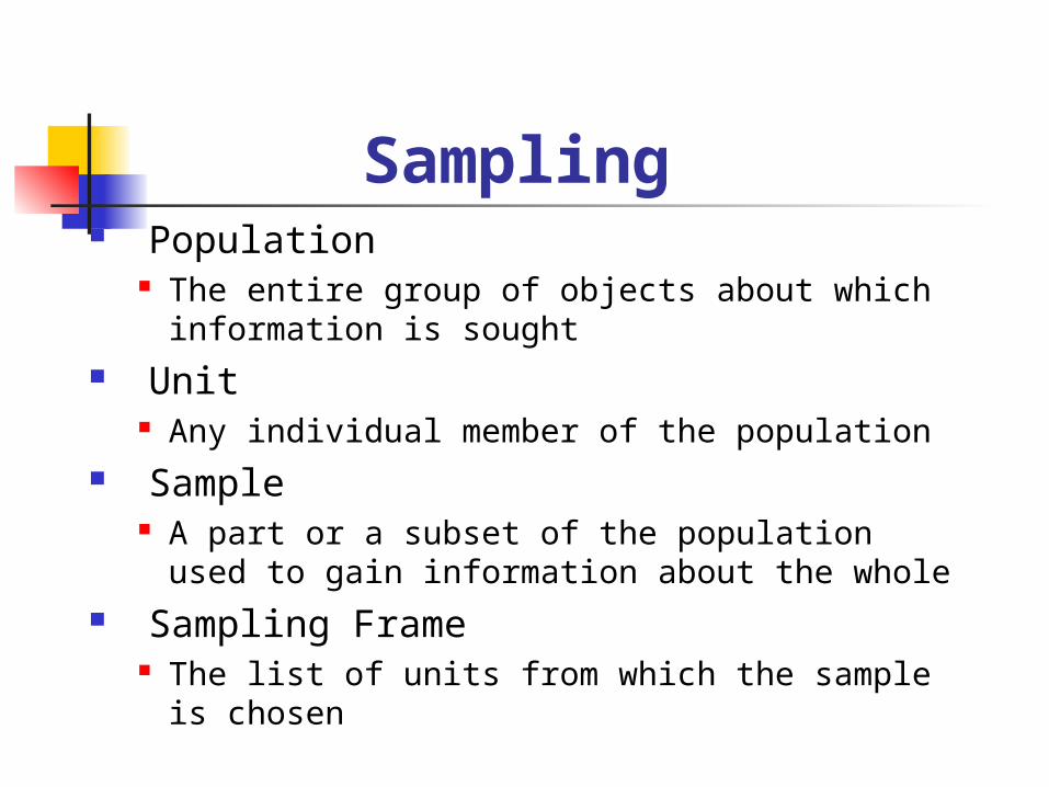
Sampling Population

The entire group of objects about which information is sought

Unit Any individual member of the population

Sample A part or a subset of the population used to

gain information about the whole Sampling Frame

The list of units from which the sample is chosen

Simple Random Sampling

A simple random sample of size n is a sample of n units chosen in such a way that every collection of n units from a sampling frame has the same chance of being chosen

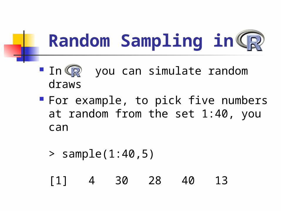
Random Sampling in R

In R you can simulate random draws

For example, to pick five numbers at random from the set 1:40, you can

> sample(1:40,5)

[1] 4 30 28 40 13

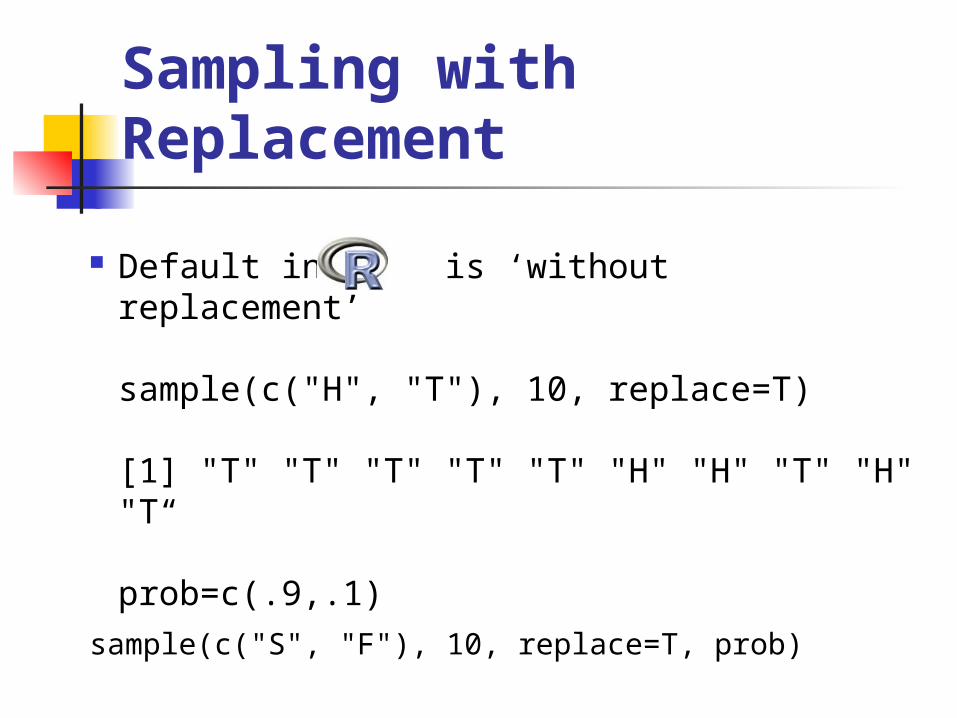
Sampling with Replacement

Default in R is ‘without replacement’

sample(c("H", "T"), 10, replace=T)

[1] "T" "T" "T" "T" "T" "H" "H" "T" "H" "T“

prob=c(.9,.1)sample(c("S", "F"), 10, replace=T, prob)

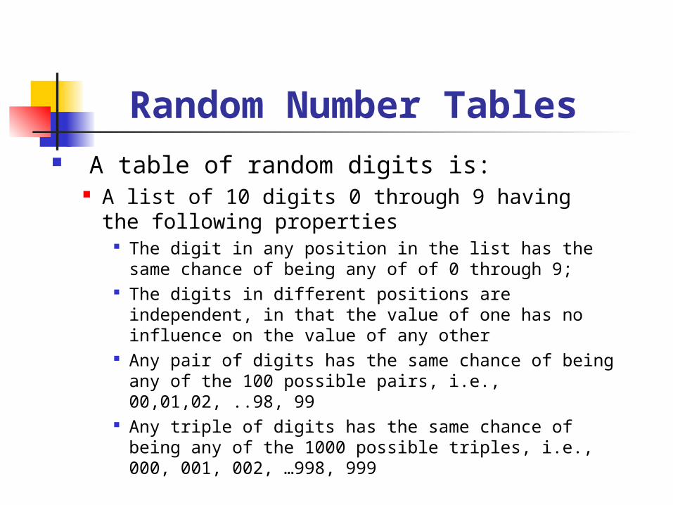
Random Number Tables A table of random digits is:

A list of 10 digits 0 through 9 having the following properties

The digit in any position in the list has the same chance of being any of of 0 through 9;

The digits in different positions are independent, in that the value of one has no influence on the value of any other

Any pair of digits has the same chance of being any of the 100 possible pairs, i.e., 00,01,02, ..98, 99

Any triple of digits has the same chance of being any of the 1000 possible triples, i.e., 000, 001, 002, …998, 999

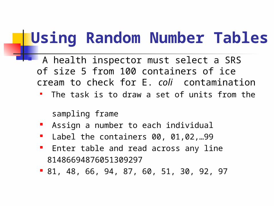
Using Random Number Tables

A health inspector must select a SRS of size 5 from 100 containers of ice cream to check for E. coli contamination

The task is to draw a set of units from the sampling frame

Assign a number to each individual Label the containers 00, 01,02,…99 Enter table and read across any line

81486 69487 6051309297

81, 48, 66, 94, 87, 60, 51, 30, 92, 97

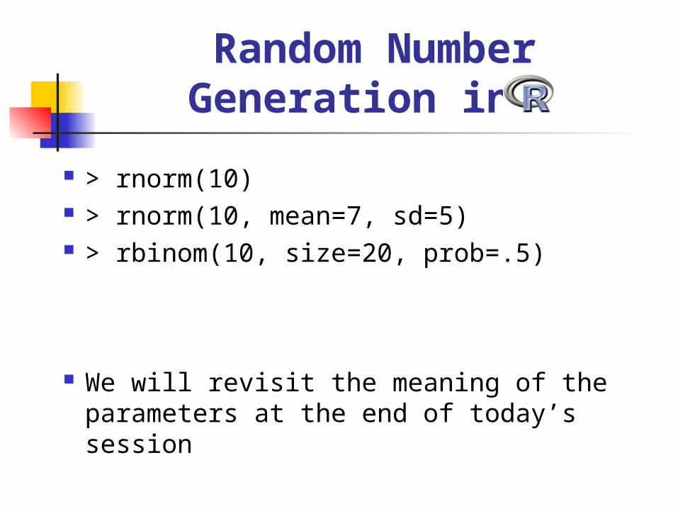
Random Number Generation in R

> rnorm(10) > rnorm(10, mean=7, sd=5) > rbinom(10, size=20, prob=.5)

We will revisit the meaning of the parameters at the end of today’s session

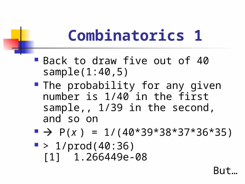
Combinatorics 1 Back to draw five out of 40

sample(1:40,5) The probability for any given

number is 1/40 in the first sample,, 1/39 in the second, and so on

P(x ) = 1/(40*39*38*37*36*35) > 1/prod(40:36)

[1] 1.266449e-08But…

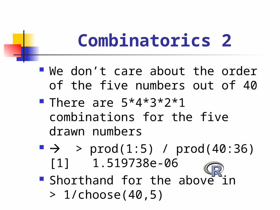
We don’t care about the order of the five numbers out of 40

There are 5*4*3*2*1 combinations for the five drawn numbers

> prod(1:5) / prod(40:36)[1] 1.519738e-06

Shorthand for the above in > 1/choose(40,5)

Combinatorics 2

Binomial Distribution

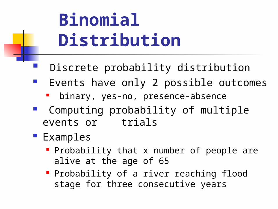
Discrete probability distribution Events have only 2 possible outcomes

binary, yes-no, presence-absence Computing probability of multiple events

or trials Examples

Probability that x number of people are alive at the age of 65

Probability of a river reaching flood stage for three consecutive years

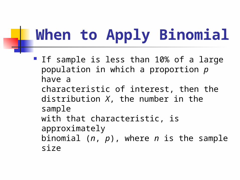
When to Apply Binomial If sample is less than 10% of a large

population in which a proportion p have acharacteristic of interest, then the distribution X, the number in the sample with that characteristic, is approximately binomial (n, p), where n is the sample size

Geometric Distribution

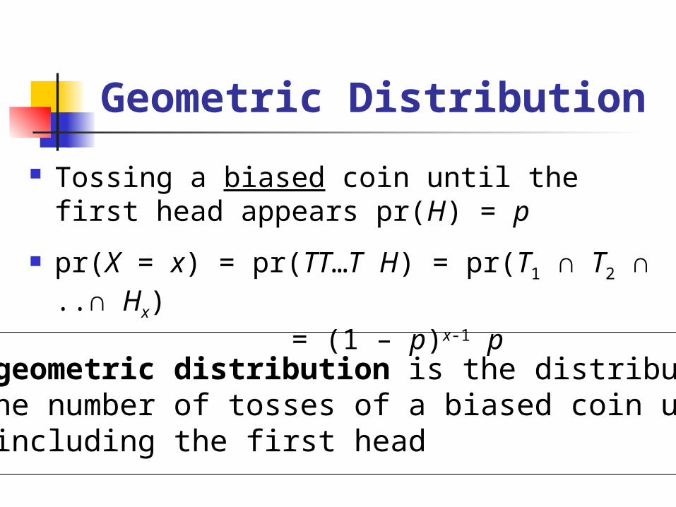
Tossing a biased coin until the first head appears pr(H) = p

pr(X = x) = pr(TT…T H) = pr(T1 ∩ T2 ∩ ..∩ Hx) = (1 – p)x-1 p

The geometric distribution is the distributionof the number of tosses of a biased coin up toand including the first head

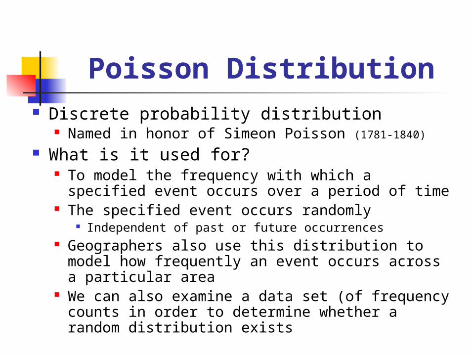
Poisson Distribution Discrete probability distribution

Named in honor of Simeon Poisson (1781-1840)

What is it used for? To model the frequency with which a specified

event occurs over a period of time The specified event occurs randomly

Independent of past or future occurrences Geographers also use this distribution to model

how frequently an event occurs across a particular area

We can also examine a data set (of frequency counts in order to determine whether a random distribution exists

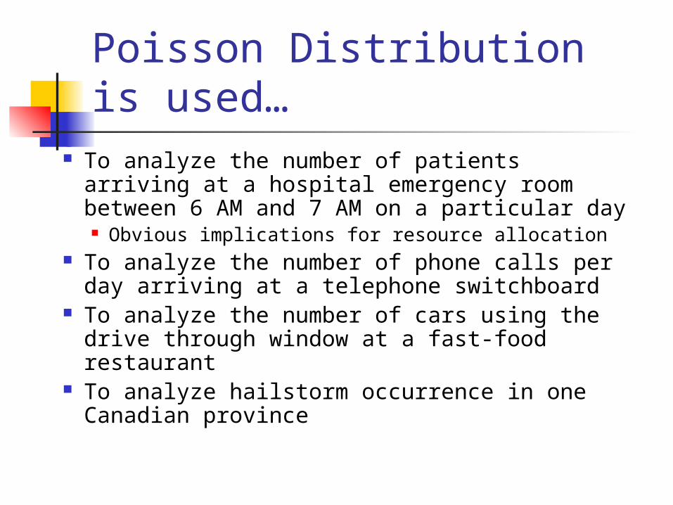
Poisson Distribution is used…

To analyze the number of patients arriving at a hospital emergency room between 6 AM and 7 AM on a particular day Obvious implications for resource allocation

To analyze the number of phone calls per day arriving at a telephone switchboard

To analyze the number of cars using the drive through window at a fast-food restaurant

To analyze hailstorm occurrence in one Canadian province

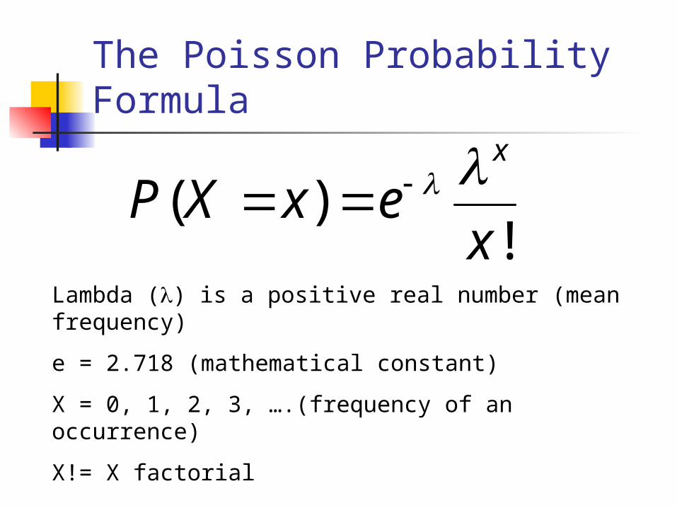
The Poisson Probability Formula

( )!

x

P X x ex

Lambda () is a positive real number (mean frequency)

e = 2.718 (mathematical constant)

X = 0, 1, 2, 3, ….(frequency of an occurrence)

X!= X factorial

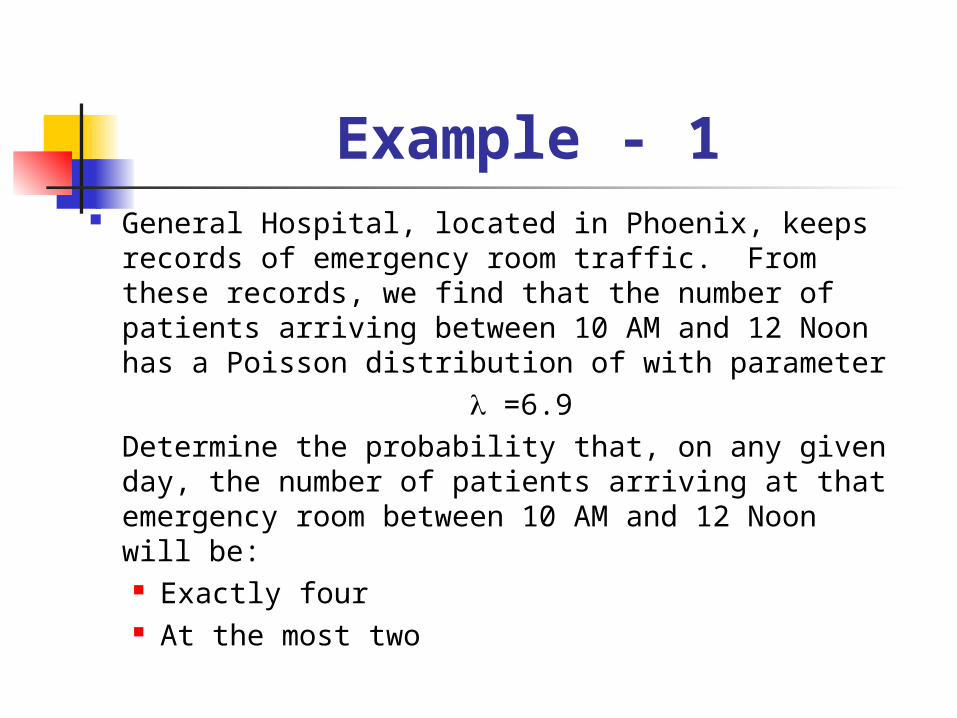
Example - 1 General Hospital, located in Phoenix, keeps

records of emergency room traffic. From these records, we find that the number of patients arriving between 10 AM and 12 Noon has a Poisson distribution of with parameter =6.9Determine the probability that, on any given day, the number of patients arriving at that emergency room between 10 AM and 12 Noon will be: Exactly four At the most two

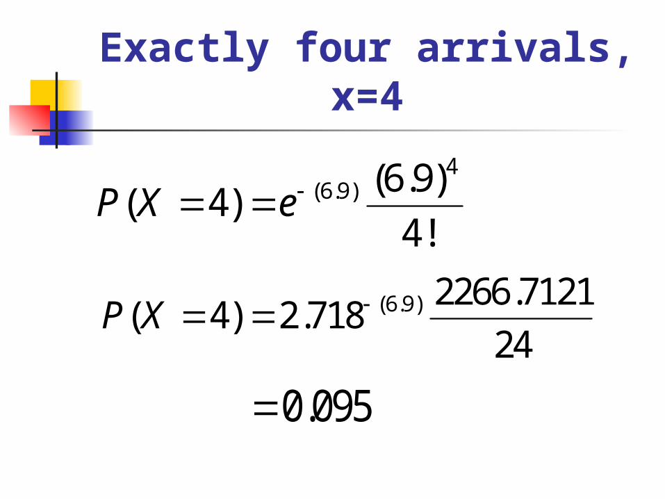
Exactly four arrivals, x=4

4(6.9) (6.9)( 4)

4! P X e

(6.9) 2266.7121( 4) 2.71824

P X

0.095

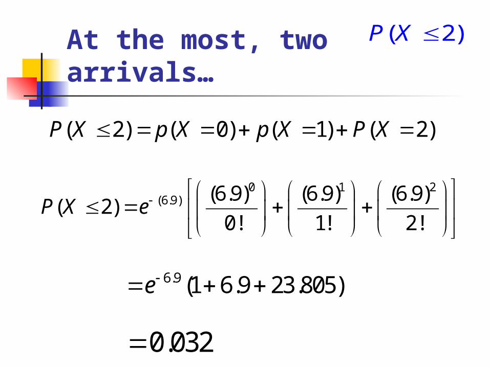
At the most, two arrivals…

( 2) ( 0) ( 1) ( 2) P X p X p X P X

0 1 2(6.9) (6.9) (6.9) (6.9)

( 2)0! 1! 2!

P X e

6.9 (1 6.9 23.805) e

0.032

( 2)P X

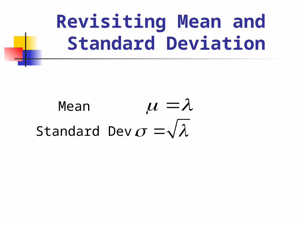
Revisiting Mean and Standard Deviation

Mean

Standard Dev.

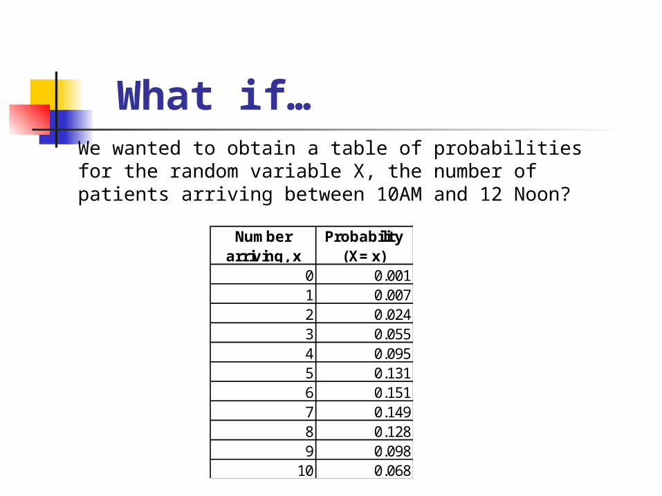
What if…We wanted to obtain a table of probabilities for the random variable X, the number of patients arriving between 10AM and 12 Noon?

Number arriving, x

Probability (X=x)

0 0.0011 0.0072 0.0243 0.0554 0.0955 0.1316 0.1517 0.1498 0.1289 0.098

10 0.068

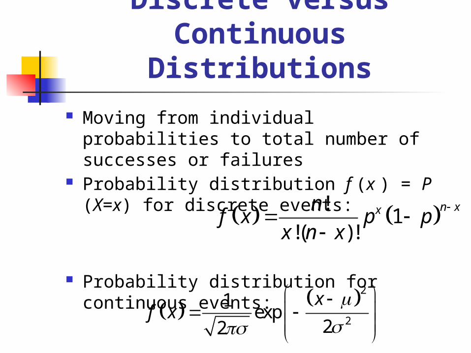
Discrete versus Continuous

Distributions Moving from individual probabilities to

total number of successes or failures Probability distribution f (x ) = P (X=x)

for discrete events:

Probability distribution for continuous events:

!1

!( )!n xxn

f x p px n x

22

1exp

22

xf x

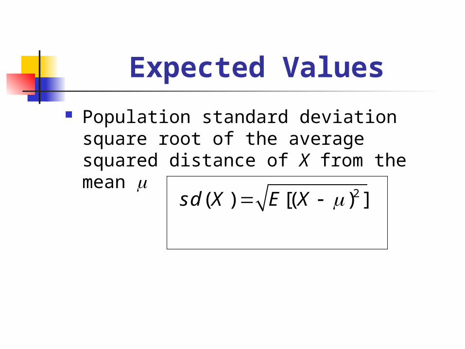
Expected Values Population standard deviation

square root of the average squared distance of X from the mean

2( ) [( ) ]sd X E X

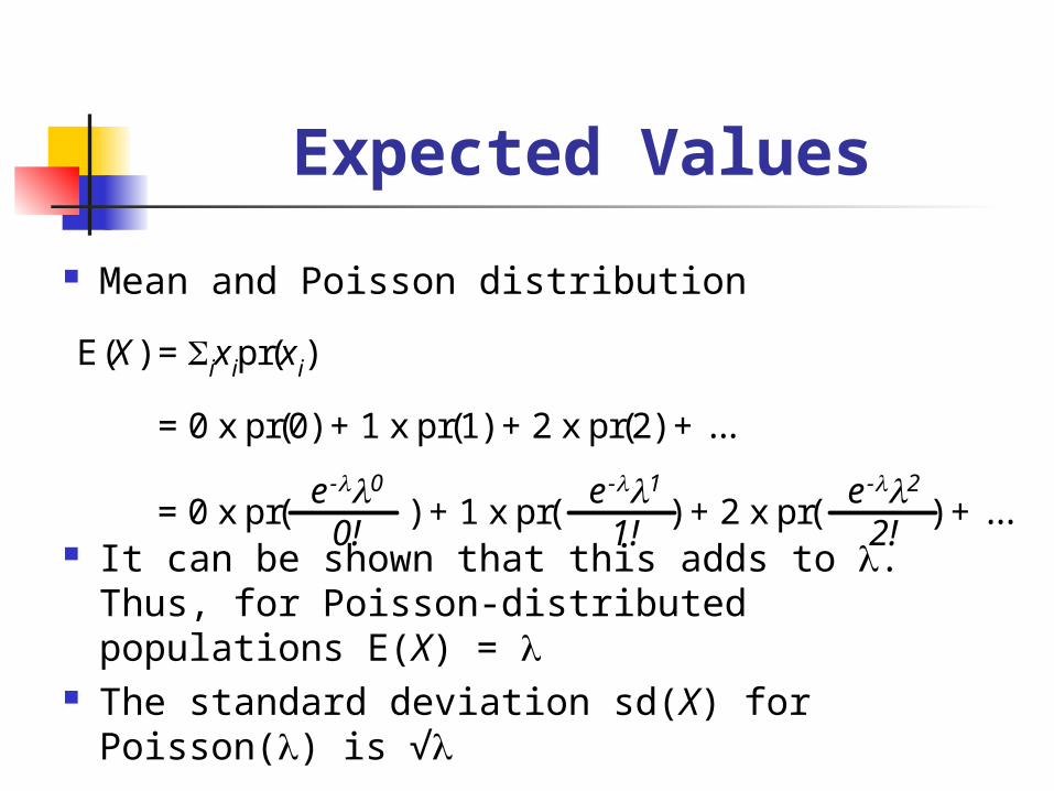
Expected Values

Mean and Poisson distribution

It can be shown that this adds to . Thus, for Poisson-distributed populations E(X) =

The standard deviation sd(X) for Poisson() is √

E(X) = ixipr(xi)

= 0 x pr(0) + 1 x pr(1) + 2 x pr(2) + ...

= 0 x pr( ) + 1 x pr( ) + 2 x pr( ) + ...e-00!

e-11!

e-22!

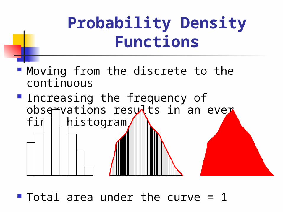
Probability Density Functions

Moving from the discrete to the continuous

Increasing the frequency of observations results in an ever finer histogram

Total area under the curve = 1

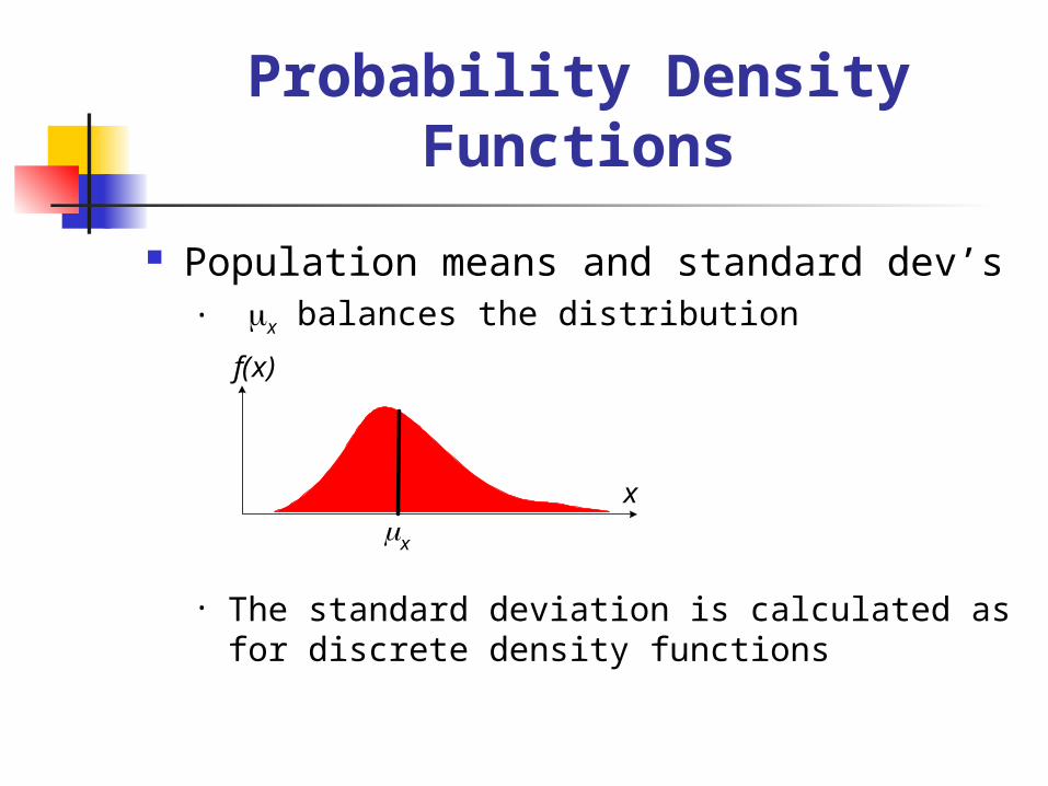
Probability Density Functions

Population means and standard dev’s• x balances the distribution

• The standard deviation is calculated as for discrete density functions

x

f(x)

x

The Normal Distribution

Properties of a Normal Distribution

Continuous Probability Distribution Symmetrical about a central point

No skewness Central point in this dataset corresponds to all

three measures of central tendency Also called a Bell Curve If we accept or assume that our data is

normally distributed, then, We can compute the probability of different

outcomes

Using the symmetrical property of the

distribution, we can conclude: 50 % of values must lie to the right, i.e. they

are greater than the mean 50% of values must lie to the left, i.e. If the data is normally distributed, the

probability values are also normally distributed

The total area under the normal curve represents all (100%) of probable outcomes

What can you say about data values in a normally distributed data set?

Properties of a Normal Distribution

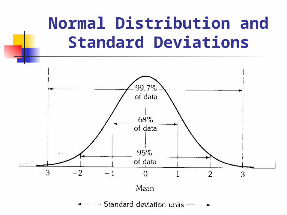
Normal Distribution and Standard Deviations

Approximating a Normal Distribution

In reality, If a variable’s distribution is shaped

roughly like a normal curve, Then the variable approximates a

normal distribution Normal Distribution is determined by

Mean Standard Deviation These measures are considered parameters

of a Normal Distribution / Normal Curve

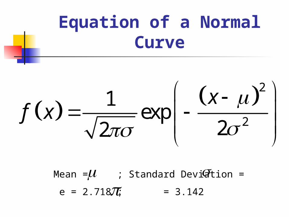
Equation of a Normal Curve

Mean = ; Standard Deviation =

e = 2.718 ; = 3.142

22

1exp

22

xf x

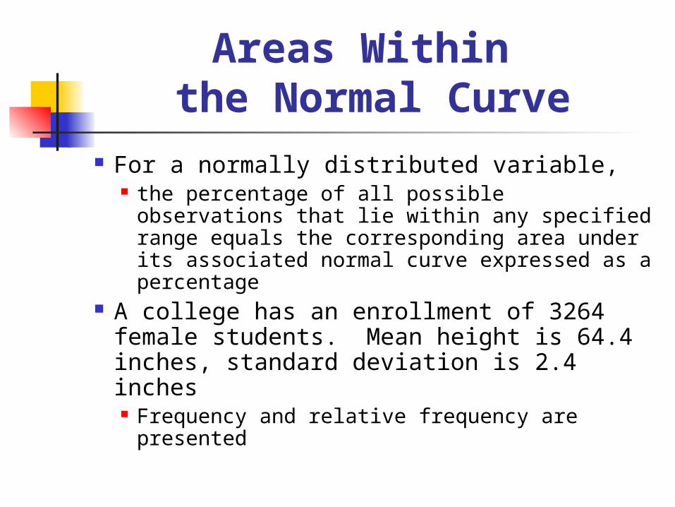
Areas Within the Normal Curve

For a normally distributed variable, the percentage of all possible observations

that lie within any specified range equals the corresponding area under its associated normal curve expressed as a percentage

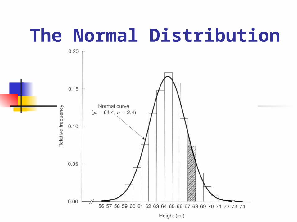
A college has an enrollment of 3264 female students. Mean height is 64.4 inches, standard deviation is 2.4 inches Frequency and relative frequency are

presented

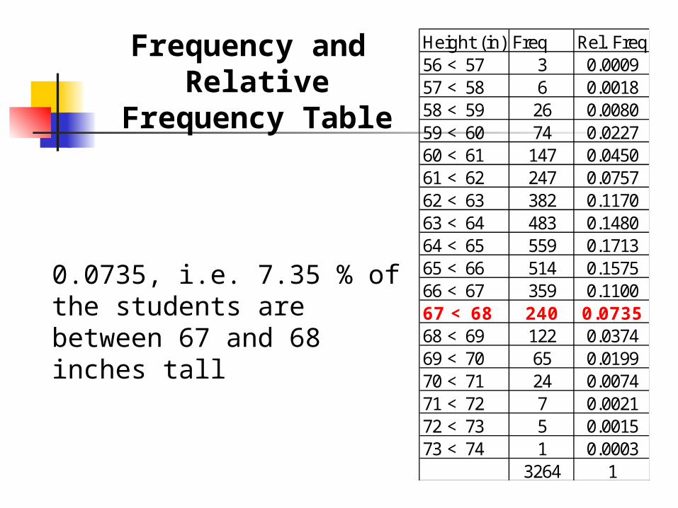
Height (in) Freq Rel. Freq56 < 57 3 0.000957 < 58 6 0.001858 < 59 26 0.008059 < 60 74 0.022760 < 61 147 0.045061 < 62 247 0.075762 < 63 382 0.117063 < 64 483 0.148064 < 65 559 0.171365 < 66 514 0.157566 < 67 359 0.110067 < 68 240 0.073568 < 69 122 0.037469 < 70 65 0.019970 < 71 24 0.007471 < 72 7 0.002172 < 73 5 0.001573 < 74 1 0.0003

3264 1

Frequency and Relative

Frequency Table

0.0735, i.e. 7.35 % of the students are between 67 and 68 inches tall

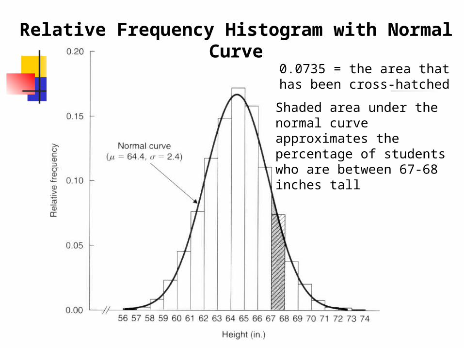
Relative Frequency Histogram with Normal Curve

0.0735 = the area that has been cross-hatched

Shaded area under the normal curve approximates the percentage of students who are between 67-68 inches tall

Standardizing a Normal Variable

Once we have mean and standard deviation of a curve, we know its distribution and the associated normal curve

Percentages for a normally distributed variable are equal to the areas under the associated normal curve

There could be hundreds of different normal curves (one for each choice of mean or std. dev. value

How can we find the areas under a standard normal curve?

A normally distributed variable with a mean of 0 and a standard deviation of 1 is said to have a standard normal distribution

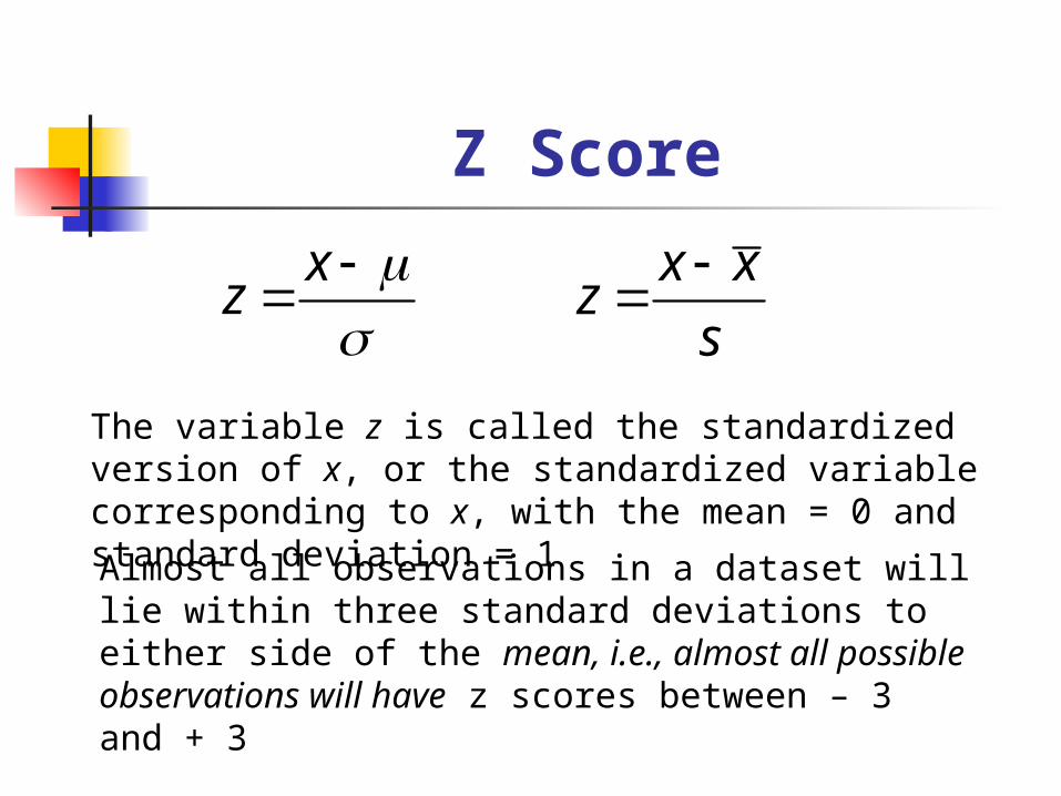
Z Score

xz

The variable z is called the standardized version of x, or the standardized variable corresponding to x, with the mean = 0 and standard deviation = 1Almost all observations in a dataset will lie within three standard deviations to either side of the mean, i.e., almost all possible observations will have z scores between – 3 and + 3

x xz

s

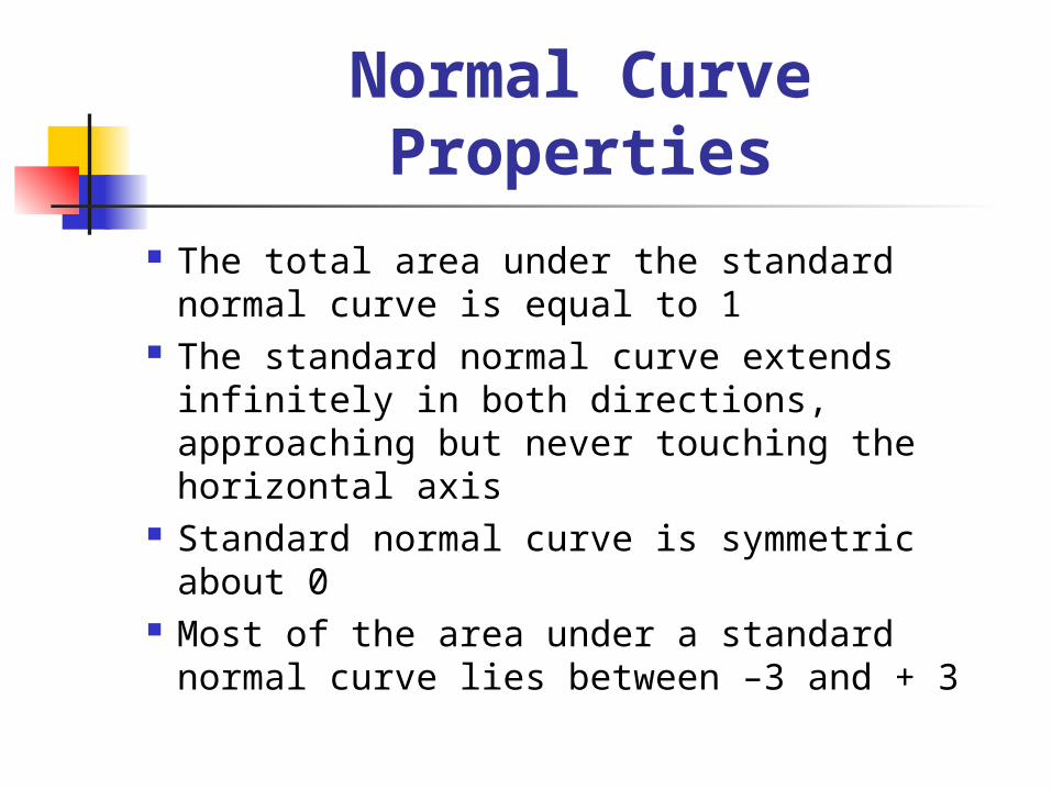
Normal Curve Properties

The total area under the standard normal curve is equal to 1

The standard normal curve extends infinitely in both directions, approaching but never touching the horizontal axis

Standard normal curve is symmetric about 0

Most of the area under a standard normal curve lies between –3 and + 3

Using the Standard Normal Table

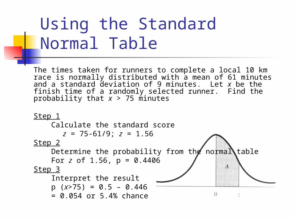
The times taken for runners to complete a local 10 km race is normally distributed with a mean of 61 minutes and a standard deviation of 9 minutes. Let x be the finish time of a randomly selected runner. Find the probability that x > 75 minutes

Step 1 Calculate the standard score

z = 75-61/9; z = 1.56Step 2 Determine the probability from the normal table For z of 1.56, p = 0.4406Step 3 Interpret the result p (x>75) = 0.5 – 0.446 = 0.054 or 5.4% chance

Using the Standard Normal Table

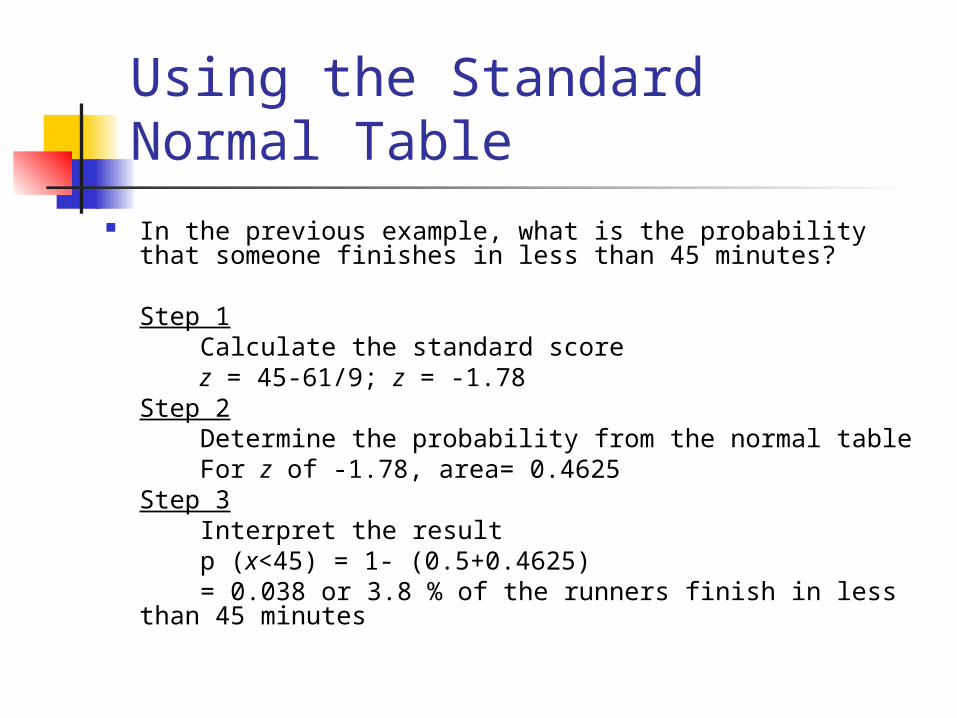
In the previous example, what is the probability that someone finishes in less than 45 minutes?

Step 1 Calculate the standard score z = 45-61/9; z = -1.78Step 2 Determine the probability from the normal table For z of -1.78, area= 0.4625 Step 3 Interpret the result p (x<45) = 1- (0.5+0.4625) = 0.038 or 3.8 % of the runners finish in less than 45 minutes

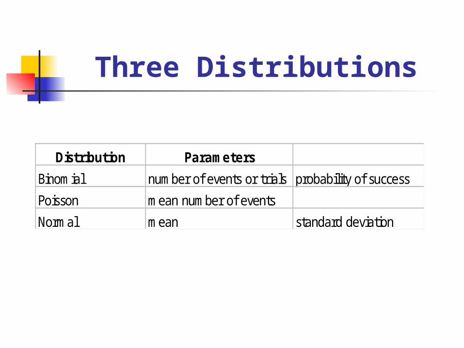
Three Distributions

Distribution Parameters

Binomial number of events or trials probability of success

Poisson mean number of events

Normal mean standard deviation

Normal Approximations for Discrete Distributions

Approximation of the Binomial Binomial is used for large n and small p If p is moderate (not close to 0 or 1),

then the Binomial can be approximated by the normal

Rule of thumb: np (1-p) ≥ 10 Other normal approximations

If X ~ Poisson(), normal works well for ≥ 10

Built-in Distributions in

Four fundamental items can be calculated for a statistical distribution: Density or point probability Cumulated probability, distribution

function Quantiles Pseudo-random numbers

In there are functions for each of these

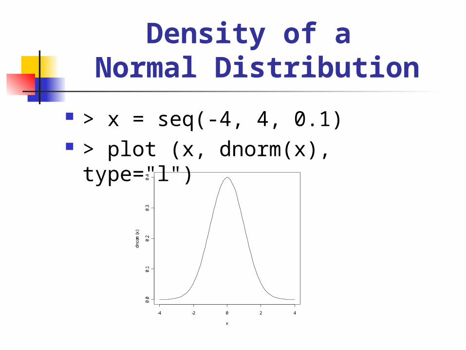
Density of a Normal Distribution

> x = seq(-4, 4, 0.1) > plot (x, dnorm(x), type="l")

-4 -2 0 2 4

0.0

0.1

0.2

0.3

0.4

x

dnor

m(x

)

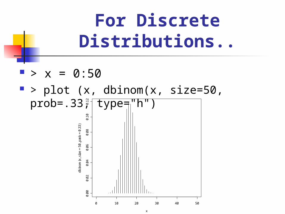
For Discrete Distributions..

> x = 0:50 > plot (x, dbinom(x, size=50, prob=.33,

type="h")

0 10 20 30 40 50

0.0

00

.02

0.0

40

.06

0.0

80

.10

0.1

2

x

dbi

nom

(x, s

ize

= 5

0, p

rob

= 0

.33)

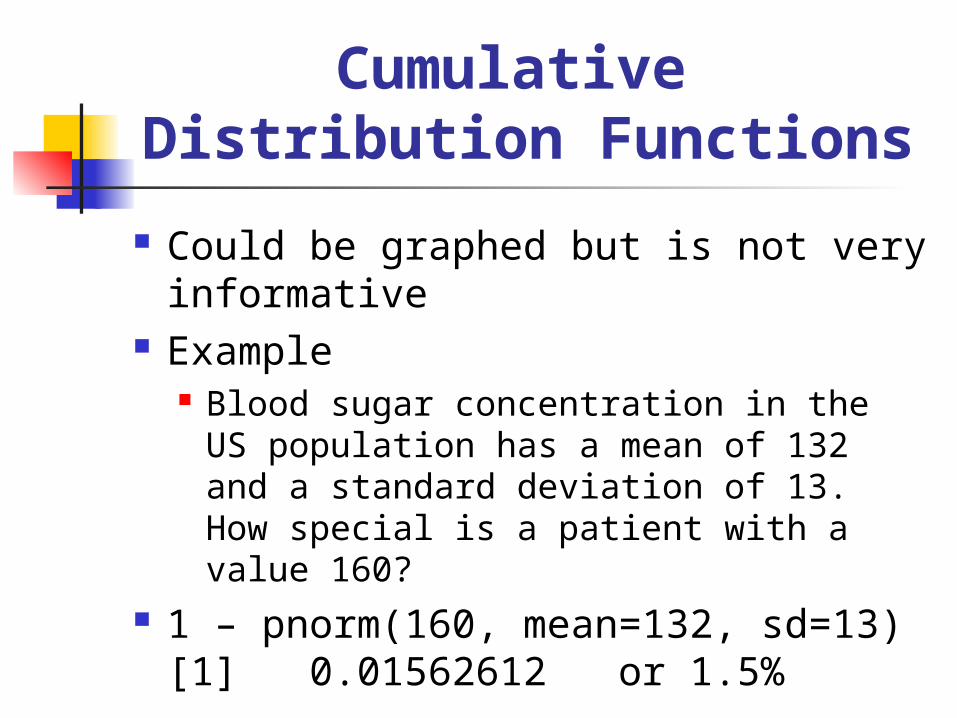
Cumulative Distribution Functions

Could be graphed but is not very informative

Example Blood sugar concentration in the US

population has a mean of 132 and a standard deviation of 13.How special is a patient with a value 160?

1 – pnorm(160, mean=132, sd=13)[1] 0.01562612 or 1.5%

Random Number Generation in R

> rnorm(10) > rnorm(10, mean=7, sd=5) > rbinom(10, size=20, prob=.5)

Now you understand the parameters…