AD-AISS 523 NOOE~M AND SATEffIIUERUAITIOIS OF 1/2LOU A PEC IAN(U LI2I U (EWGAD

0 OGGJAHf A HN~Q4SLE UAL. MUr8

UNCLASSIFIED M -R -IAOS-- t' 4/r NL

p 6*

tv

lb UV W8

Contract/Grant Number APOSR-86-0299

HOMOGENIZING SURFACE AND SATELLITE OBSERVATIONS OF CLOUD:

ASPECTS OF BIAS IN SURFACE DATA

A. Hendermon-Sellr and A.H. GoodmanDepartment of GeographyUniversity of LiverpoolLiverpool, U.K.

(V)

CM November 1987In

0~Mm Interim Scientific Report, I October 1986 - 30 September 1987

Approved for public release; distribution unlimited

Prepared for

EUROPEAN OFFICE OF AEROSPACE RESEARCH AND DEVELOPMENT

DTICELECfTE

R1~IIDEC 22W

860

87121608

R DREAD INSTRUCTIONS

REPp T DOCUENTATION PAGE BEFORE COMPLETING FORM

t R2. Govt Accession No. 3. Recipient's Catalog Number

EOARDTR-87- I:4. Title (and Subtitle) 5. Type of Report & Period CoveredHomogenizing surface and satellite Interim, 1 October 86observations of cloud: aspects of 30 September 87.bias in surface data.

6. Performing Org. Report Number

7. Author(s) 8. Contract or Grant NumberAnn Henderson-Sellers and Alan Goodman AFOSR-86-0299

9. Performing Organization Name and Address 10. Program Element, Project, TaskDepartment of Geography, Area & Work Unit NumbersUniversity of Liverpool,P.O. Box 147,Liverpool, L69. 3BX.

11. Controlling Office Name and Address 12. Report DateEOARD 10 November 1987223/231 Old Marylebone Road,London, NW1, 5TH U.K. 13. Number of Pages

12814. Monitoring Agency Name and Address 15.

16. & 17. Distribution Statement

Approved for public release; distribution unlimited.

18. Supplementary Notes

19. Key WordsBias, partial undercast, night-time bias of surface observers,okta observing scale.

20. AbstractA global, surface-observed cloud data set supplied by the U.S.

Air Force for the months of July 1983 and January 1985 wasinvestigated i) for evidence of night-detection bias in whichobservers may be repeatedly failing to discern the presence ofcirrus and altostratus during darkness, ii) to assess the impactof the "partial undercast" bias and iii) to check for anysignificant bias effects arising from the definitions of 1 and 7oktas cloud amount. Several well-spaced regions of the world wereused as study areas in all 3 cases.

In case i) diurnal analyses of the frequency of occurrence ofcirrus and altostratus were used to check for sunrise/sunset ordaytime peaks which might have indicated anomalously high (low)values during daytime (night-time). Attention was particularly paidFM 1473 AlO-

Dlstrlbutlo/

Availability Codesarea Avall and/or

Dist JSpecilj

eIWode

!r

SgCumv CLASSFjCA'TgO OW VNI$ PAGC'Wh u D* £EAWed,

20. Abstract cont,d ............

to the 100 x 200 analysis region over Scandinavia where the large

change in daylength between January and July would be expected to

accentuate any bias present. Analysis within the study areas was

repeated on small groups of stations within smaller areas to see

whether the results were reproduced over smaller scales. It was

found that the effects of bias may be stronger for small

localities rather than over large areas. Only in the

Scandinavian region was a significant diurnal variation

identifiable for larger scales (0 0 x 200). Supplementary diurnal

analyses which may have helped to confirm any bias are included.

Partial undercast bias arises in situations in which upper

cloud layers are present but are invisible to the observer as

they do not encroach into any clear areas of the sky and therefor

go unreported. In case ii) contingency probabilities which

express the likelihood that given one cloud type another is

present, were introduced in an attempt to confirm their potential

use in such cases, as has been previously suggested. In the

literature values of contingency probability for pairs of lower

and upper cloud types have been shown to remain fairly steady

over the range of partial undercast lower cloud amounts (i.e.

1-7 oktas). The results presented here showed a general decrease

in contingency probability for increasing lower cloud amountsimplying that the likelihood of the presence of upper cloudsdecreased as the lower cloud amount increased, a resultinconsistent with previous assertions.

Possible biases arising out of the WMO definitions of 1 and

7 oktas were investigated with the aid of histograms showing the

frequency with which each value on the okta scale is reported.Very low relative frequencies of 0:1 oktas indicate a situation

in which the frequency of cloud amounts much less than I okta

exceeds the frequency with which approximately I okta is actually

present, causing an overestimate in the long term value of cloui

amount. Such occurrences were found in several instances.

Similarly very high relative frequencies of 7:8 oktas mightsuggest cases where the majority of 7 okta reports correspond to

tiny gaps or suspected gaps in the cloud deck, causing an

underestimate in the long term cloud amount. No instances of

the latter were recorded.

The global data set was then used to construct a series of

maps for the land and ocean describing the frequency of

occurrence of cloud types, total and level cloud amounts and

examples of contingency probabilities. The maps are presented

and discussed in the context of their uspfulness and in

comparison to other data.

C%. -51ICTf 4W

Contents

Page

1. Introduction 3

2. Analysis of January 1965 and July 1983

surface observatlons for evidence of bias 4

2.1 Introduction 4

2.2 Data Source 14

2.3 Night Detection Bias 14

2.4 Discussion of Results 17

2.5 Other Methods of Detecting Nighttime Bias 25

2.6 The use of Contingency Probabilities for situations of

Partial Undercut Bias 37

2.7 Results 4 1

i)L = St/Sc, U = Ac/As 41

ui)L = St/ScU = i/Cs/Cc 46

2.8 1 and 7 okta bias 53

3. Global evaluation at surface cloud observatlonas 58

3.1 Data 58

8.2 BDim within the observations 59

3.8 alyb Procedure , 6 1

i) ztraction o Required Information 61

ii) Cloud Type Categories 62

iii) ClAud Amounts 62

..__ __ E

iv) Prequency of occurrenc of cloud types 6

v) aEcive Probabiliy 65

vi) Contiasancy Probabiliti6s

3.4 Map foimast 67

3.5 Discueuion 69

4. Summary and Cwonlloma 123

5. Pnesulatlows and publications 1 211

R. 3gremceg 125

'AA

Abstract

A global, surface-observed cloud data met supplied by the U.S. Air Force for the months of July

1963 and January 1985 was investigated i) for evidence of night-detection bias in which observers

may be repeatedly failing to discern the presence of cirrus and altostratus during darkness, ii) to

assem the impact of the "partial undercast" bias and iii) to check for any significant bias effects

arising from the definitions of I and 7 oktas cloud amount. Several well-spaced regions of the world

were used as study areas in all 3 cases.

In case i) diurnal analyses of the frequency of occurrence of cirrus and altostratus were used

to check for sunrise/sunset or daytime peaks which might have indicated anomalously high (low)

values during daytime (nighttime). Attention was particularly paid to the 10O x 200 analysis region

over Scandinavia where the large change in daylength between January and July would be expected

to accentuate any bias present. Analysis within the study areas was repeated on small groups of

stations within smaller areas to see whether the results were reproduced over smaller scales. It

was found that the effects of bias may be stronger for small localities rather than over large areas.

Only in the Scandinavian region was a significant diurnal variation identifiable for larger scales

(10* x 201). Supplementary diurnal analyses which may have helped to confirm any bias are

included.

Partial undercast bias arises in situations in which upper cloud layers are present but are

invisible to the observer as they do not encroach into any clear areas of the sky and therefore

go unreported. In case ii) contingency probabilities which express the likelihood that given one

cloud type another is present, were introduced in an attempt to confirm their potential use in

such cases, as has been previously suggested. In the literatura values of contingency probability

for pairs of lower and upper cloud types have been shown to remain fairly steady over the range

of partial undereast lower cloud amounts (i.e. 1-7 oktas). The results presented hes showed a

general decrease in cotingency probability for incresmng lower cloud amunts implying that the

-- - - - k ,. . , " '

likelihood of the presence of upper clouds decreased as the lower cloud amount increased, a result

inconsistent with previous assertions.

Possible biases arising out of the WMO definitions of 1 and 7 oktas were investigated with the

aid of histograms showing the frquency with which each value on the okta scale is reported. Very

low relative frequencies of 0:1 oktas indicate a situation in which the frequency of cloud amounts

much less than I okta exceeds the frequency with which approximately 1 okta is actually present,

casing an overestimate in the long term value of cloud amount. Such occurrences woe found in

several instances. Similarly very high relative frequencies of 7:8 oktas might suggest cams where

the njority of 7 okta reports correspond to tiny gaps or suspected gaps in the cloud deck, causing

an underestimate in the long term cloud amount. No instances of the latter were recorded.

The global data set was then used to construct a series of maps for the land and ocean

describing the frequency of occurrence of cloud types, total and level cloud amounts and examples

of contingency probabilities. The maps are presented and discussed in the context of their usefulness

and in comparison to other data.

2

1. Introductlon

The meteorological community is at present placing great emphasis on the analysis of clouds

and their configurations from satellite imagery, much effort being devoted to the improvement of

the accuracy and performance of retrieval algorithms (Roesow et a1., 1985; Arking and Childs,

1985; Chou et aL, 1986; Saunders and Kriebel, 1987; Coakley, 1987). The superior coverage

afforded by satellites as compared to the uneven distribution of ground stations throughout the

world and their scarcity over oceanic and polar regions is one of the chief causes of this trend. The

satellite era now permits the remotely-sensed measurement of cloud optical parameters affecting the

radiation budgets of the Earth and atmosphere to be achieved (e.g. Chahine, 1982) and methods

for estimating cloud cover fraction from satellite radiance data are well documented in the literature

(Reynolds and Vonder Haar, 1977; Coakley and Bretherton, 1982; Saunders, 1986), whilst schemes

aiming to deduce the exact cloud types are now also developed (Desbois et at., 1982; Lilias, 1984,

1986).

From a surface viewpoint reports of cloud type are still more reliable than those from above;

the observer on the ground is that much closer to the clouds and is able to resolve individual clouds

within his field of vision. Such data, describing the amount and type of cloud present, are still the

only feasible means of validating and comparing remotely sensed cloud information (Henderson-

Sellers et at., 1987), also serving as sources of input and comparative data for the purposes of

climate models. With the latter in mind, attention has been paid to evaluating global surface data

not only in the form of amount climatologies (Berlyand and Strokina, 1980) but also in terms of the

frequency of occurrence of the various cloud types, their individual amounts and the modes in which

combinations oftypes occur together (Hahn et @L, 192, 1984; Warren et &L, 1986, 1967). (A recent

review of global cloud climatologis is given in Hughes (1984)). The International Satellite Cloud

Climatology Project (ISCCP) will shortly be providing satellite retrievals against which comparative

ad validatory exercises should take place whilst surfice observations are alredy providing a maor

.... . .. . .---. .... t= i d~amd. d~i.......... -

component to the First ISCCP Regional Experiment (FIRE) (Cox et l., 1987). With the above

considerations in mind, particularly the likelihood of satellite-surface intercomparison, surface data

for two separate months during ISCCP (July 1983 and January 1985) have been evaluated. Section

2 describes the analysis of this surface data set for the evidence of biases of different types and

Section 3 describes a global scale evaluationof these surface observations of cloudines. Section 4

contains a summary and conclusions and Section 5 a list of presentations and publications made

this year.

2. Analysis of data set for evidence of bias

2.1 Introdectioa

Surface observations of clouds are routinely made worldwide either at land-based stations,

on ships or from aircraft. In a typical case the obeerver records the total cloud amount present

(also known as the skycover), i.e. the fraction of the celestial dome covered by cloud, along with

each cloud type and the amount of each type. With a little experience estimating the skycover

and identifying the cloud types visible is a relatively straightforward task. The ease with which

a full description of the clouds can be given, however, depends on the types present and their

relative configuration, as well as the experience, location and procedure adopted by the observer.

Where the clouds exhibit vertical development the observer includes the sides s well as the bases

of the clouds in his entimate of the total cloud amount (the skycover) (Figure 1) (Malberg, 1973),

overestimating with respect to a satellite viewing the same area which would observe only the

vertical projection of the clouds against the Earth (termed the earthcover). It is very important to

recognise that surface observations made correctly are not overestimates; they are accurate reports

of rycover. The tems over- and under-estimation enter descriptions, ohen inappropriately, when

skycover and earthcover ae compared without due evaluation of the definition of the tertn.

. . . . . ... .. .. . ..b_ , ' . ' . '

04 0 CLOD GVOJ/

Fiu 1/srtc fhwa bevrss h ie swHa h ae fvrk~-eeoe

N~ud /hnMle,17)

N /~

Both surface and matellite observations may overestimate the cloud amount in situations when

the clouds adopt regular arrays interspersed by small gaps as with stratocumulus and altocumulus.

In such cases those gaps close to the horizon will not be detected. The quality of surface cloud

observations is further affected by the fact that on many occasions the clouds comprise several

types of differing amount and at various heights. In a multilayered situation the observer cannot

always discern even the presence of middle or upper level clouds, let alone their amounts, due to

obscuration by lower layers. Observations of clouds at night are especially difficult. The lack of

illumination makes it hard for the observer to identify individual types (especially cirrus) and their

respective amounts, even after he has accustomed his eye to the dim light.

The above points illustrate some of the problems encountered with surface-based cloud obser-

vations. In general, though, they provide relatively accurate estimates of low and total skycover

and of cloud types. Prior to the advent of the satellite retrieval techniques they were the principal

source of global cloud statistics and all cloud climatologies compiled in this period used ground-

based reports (Brooks, 1927; London, 1957; Hastenrath and Lamb, 1977). Indeed, in the absence

of a satellite-based global cloud climatology (Schiffer and Rossow, 1983), surface observations have

often been deemed useful enough to be incorporated into climate models as both input and in

validations. They also form a significant data component for the U.S. Air Force's nephanalysis

(Fye, 1978; Henderson-Sellers and Hughes, 1985). Nevertheless, the potential biases inherent in

such data require careful attention. Only recently, however, has this been forthcoming in the work

of Hahn et at. (1962, 1984) and Warren et aL (1986), which introduced the concept of contingency

probabilities as part of their overall description of the global cloud field as observed from the

surface and whoe work provided part of the motivation for this investigation. Nighttime bias,

partial undercut bis and 1,7 okta bias were selected as study topics and the following sections

detail the analysis of each type of bias.

6

Table I Low level cloud classification (CL) as defined by WMO (from WMO, 1984)

CL - Clouds of the genera Stratocumulus, Stratus, Cumulus and Cumulonimbus

Code Technical specifications Code Non-technical specifications

0 No CL clouds 0 No Stratocumulus, Stratus, Cumulus or Cum-

ulonimbus1 Cumulus humilis or Cumulus fractus 1 Cumulus with little vertical extent and seem-

other than of bad weather,* or both ingly flattened, or ragged Cumulus other than

of bad weather, * or both2 Cumulus mediocris or congestus, with or 2 Cumulus of moderate or strong vertical extent,

without Cumulus of species fractus or hu- generally with protuberances in the form of

milis or Stratocumulus, all having their domes or towers, either accompanied or not by

bases at the same level other Cumulus or by Stratocumulus, all hav-

ing their bases at the same level3 Cumulonimbus calvus, with or without 3 Cumulonimbus the summits of which, at least

Cumulus, Stratocumulus or Stratus partially, lack sharp outlines, but are neither

clearly fibrous (cirriform) nor in the form of

an anvil; Cumulus, Stratocumulus or Stratus

may also be present4 Stratocumulus cumulogenitus 4 Stratocumulus formed by the spreading out of

Cumulus; Cumulus may also be present

5 Stratocumulus other than Stratocumulus 5 Stratocumulus not resulting from the spread-

cumulogenitus ing out of Cumulus6 Stratus nebulosus or Stratus fractus other 6 Stratus in a more or less continuous sheet or

than of bad weather,* or both layer, or in ragged shreds, or both, but no

Stratus fractus of bad weather*

7 Stratus fractus or Cumulus fractus of bad 7 Stratus fractus of bad weather* or Cumulus

weather,* or both (pannus), usually below fractus of bad weather, or both (pannus), usu-

Altostratus or Nimbostratus ally below Altostratus or Nimbostratus8 Cumulus and Stratocumulus other than 8 Cumulus and Stratocumulus other than that

Stratocumulus cumulogenitus, with bass formed from the spreading out of Cumulus;

at difierent levels the base of the Cumulus is at a different level

from that of the Stratocumulus

7

9 Cumulonimbus capillatus (often with an 9 Cumulonimbus, the upper part of which isanvil), with or without Cumulonimbus clearly fibrous (cirriform), often in the formcalvus, Cumulus, Stratocumulus, Stratus of an anvil; either accompanied or not by Cu-or pannus mulonimbus without anvil or fibrous upper

part, by Cumulus, Stratocumulus, Stratus or

pannusCL clouds invisible owing to darkness, fog, / Stratocumulus, Stratus, Cumulus and Cu-blowing dust or sand, or other similar mulonimbus invisible owing to darkness, fog,

phenomena blowing dust or sand, or other similar pheno-

mena

"Bad weather" denotes the conditions which generally exist during precipitation and a short time before and after.

I8

Table 2 Middle level cloud classification (Cm) as defined by WMO (from WMO,

1984)

Cm - Clouds of the genera Altocumulus, Altostratus and Nimbostratus

Code Technical specifications Code Non-technical specifications

0 No CM clouds 0 No Altocumulus, Altostratus or Nimbostratus

I Altostratus tranalucidus 1 Altostratus, the greater part of which is semi.transparent; through this part the sun or

moon may be weakly visible, as through

ground glass2 Altostratus opacus or Nimbostratus 2 Altostratus, the greater part of which is suf-

ficiently dense to hide the sun or moon, or

Nimbostratus

3 Altocumulus translucidus at a single level 3 Altocumulus, the greater part of which is semi-transparent; the various elements of the cloud

change only slowly and are all at a single level4 Patches (often lenticular) of Altocumulus 4 Patches (often in the form of almonds or

translucidus, continually changing and fishes) of Altocumulus, the greater part of

occurring at one or more levels which is semi-transparent; the clouds occur atone or more levels and the elements are con-

tinually changing in appearance5 Altocumulus translucidus in bands, or 5 Semi-transparent Altocumulus in bands, or

one or more layers of Altocumulus trans - Altocumulus, in one or more fairly continu-

lucidus or opacus, progressively invading ous layer (semi-transparent or opaque), pro-

the sky; these Altocumulus clouds gener- gressively invading the sky: these Altocumulus

ally thicken as a whole clouds generally thicken as a whole6 Altocumulus cumulogenitus (or cumulo- 6 Altocumulus resulting from the spreading out

nimbogenitus) of Cumulus (or Cumulonimbus)7 Altocumulus translucidus or opacus in 7 Altocumulus in two or more layers, usually

two or more layers, or Altocumulus opa- opaque in places, and not progressively invad-

cue in a single layer, not progressively in- ing the sky; or opaque layer of Altocumulus,

vading the sky, or Altocumulus with Alto. not progressively invading the sky; or Alto-

stratus or Nimbostratus cumulus together with Altostratus or Nimbo-

stratus

9

• dJ mmS-memmme um -J - I

8 Altocumulus castellanus or floccus 8 Altocumulus with sproutinp in the form of

small towers or battlements, or Altocumulus

having the appearance of cumuliform tufts

9 Altocumulus of a chaotic sky, generally at 9 Altocumulus of a chaotic sky, generally at sev-

several levels eral levels/ Cu clouds invisible owing to darkness, / Altocumulus, Altostratus and Nimbostratus

fog, blowing dust or sand, or other sim- invisible owing to darkness, fog, blowing dust

ilar phenomena, or because of continuous or sand, or other similar phenomena, or more

layer of lower clouds often because of the presence of a continuous

layer of lower clouds

I10

.4i " i I a i f H ,m] , ,,N . o

Table S High level cloud classification (CH) as defined by WMO (from WMO, 1964)

CH - Clouds of the genera Cirrus, Cirrocumulus and Cirrostratus

Code Technical specifications Code Non-technical specifications

0 No CH clouds 0 No Cirrus, Cirrocumulus or Cirrostratus

1 Cirrus fibratus, sometimes uncinus, not 1 Cirrus in the form of filaments, strands or

progressively invading the sky hooks, not progressively invading the sky2 Cirrus spissatus, in patches or entangled 2 Dense Cirrus, in patches or entangled sheaves,

sheaves, which usually do not increase which usually do not increase and sometimes

and sometimes mom to be the remains seem to be the remains of the upper part of

of the upper part of a Cumulonimbus; or a Cumulonimbus; or Cirrus with sproutings in

Cirrus castellanus or floccus the form of small turrets or battlements, or

Cirrus having the appearance of cumuliform

tufts3 Cirrus spiesatus cumulonimbogenitus 3 Dense Cirrus, often in the form of an anvil, be-

ing the remains of the upper parts of Cumulo-

nimbus4 Cirrus uncinus or fibratus, or both, pro. 4 Cirrus in the form of hooks or of filaments,

gressively invading the sky; they generally or both, progressively invading the sky; they

thicken as a whole generally become denser as a whole5 Cirrus (often in bands) and Cirrostratus, 5 Cirrus (often in bands converging towards one

or Cirrostratus alone, progressively invad- point or two opposite points of the horizon)

ing the sky; they generally thicken as a and Cirrostratus, or Cirrostratus alone; in ei-

whole, but the continuous veil does not ther case, they are progressively invading the

reach 45 degrees above the horizon sky, and generally growing denser as a whole,

but the continuous veil does not reach 45 de-

grees above the horison6 Cirrus (often in bands) and Cirrostratus, 6 Cirrus (often in bands converging towards one

or Cirrostratus alone, progressively invad. point or two opposite points of the horizon)

ing the sky; they generally thicken as a and Cirrostrjtus, or Cirrostratus alone; in ei-

whole; the continuous veil extends more ther case, they are progresively invading the

than 45 degrees above the horison, with- sky, and generally growing denser as a whole;

out the sky being totally covered the continuous veil extends more than 45 de-

grew above the horizon without the sky being

totally covered

11

7 Cirrostratus covering the whole sky 7 Veil of Cirrostratus covering the celestial dome

8 Cirrostratus not progremively invading 8 Cirrostratus not progressively invading the sky

the sky and not entirely covering it and not completely covering the celestial dome9 Cirrocumulus alone, or Cirrocumulus pre- 9 Cirrocumulus alone, or Cirrocumulus accom-

dominant among the CH clouds panied by Cirrus or Cirrostratus, or both, but

Cirrocumulus is predominantCu clouds invisible owing to darkness, Cirrus, Cirrocumulus and Cirrostratus invis-

fog, blowing dust or sand, or other simi- ible owing to darknem, fog, blowing dust or

lar phenomena, or because of a continuous sand, or other similar phenomena, or more of-

layer of lower clouds ten because of the presence of a continuous

layer of lower clouds

12

Table 4 Catgrie of Observation Type In Data Set

4) Lad

i) Synoptic

ii) Airways

ii) metar

iv) Synoptic-Airways merged

v) Synoptic-metur merged

vi) Aero

vii) SMARS

viii) Synoptic-Aero merged

b) sea

i) Synoptic

13

2.2 Daa Source

The cloud data formed part of the global surface weather data set for the months of July 1983

and January 1985 and were obtained from the U.S. Defense Department via the Department of the

Air Force. They include observations taken on land (from the World Meteorological Organisation

(WMO) ground station network) and at sea. AD ship-based observations are of the conventional

synoptic type whilst those derived from land stations comprise several categories of report, de-

pending upon source, predominantly synoptic but including such categories as airways and met.r

where the report has originated from airfields and is issued with respect to aircraft flight conditions.

In some cases composite reports have been supplied by 'merging', for example an airway's report

with the corresponding synoptic observation. The categories vary in the frequency and amount

of data supplied but are given an equal weighting in the investigation. Maps showing the global

distribution of the various types of report for both months can be found in Section 3. Table 4 lists

each catory.

All cloud observations are coded according to the WMO synoptic code (WMO, 1956, 1974,

1964, 1987) which assigns the clouds to three levels (low, middle and high) and a number in the

range 0-9 for each level according to the type of cloud present (or absent) at that level. The code

255 refers to missing information about a cloud level, usually as a result of obscuration either by

precipitation or by lower layers of cloud. The classification of cloud types for each level is given in

Tables 1-3. Each report contains information on the total cloud amount and, where possible, on

the amount of each type present.

2.8 Night Detectio. Wi..

It is a matter of synoptic experience that the observation of clouds during darkness is a harder

tosk than during daylight hours. The presence of moonlight may alleviate the difficulties somewht,

equsutly enabling the observer to detect altostratus and altocumulus but in the absence of this the

• n dn nn ~ u em ,6u.* . .. ..14

observing procedure becomes eve more subjective, particularly when dealing with cloud amount.

Cirrus and altostratus re two of the types observers find hardest to detect at night particularly

when they are present as part of a multilayered cloud scene and are partially obscured by lower

layers. Even in the absence of other clouds the presence of thin cirrus by itself is Ird to discern.

Since cloud climatologes require nighttime observations in order to be fully representative it is

possible that such bins, if repeated over a significant time period, would seriously reduce the quality

of the climatology.

Riehl (1947), describing diurnal variations in cloudiness over the subtropical Atlantic, was

probably the first to suggest a possible underestimate of cirrus by observers during nighttime.

Normally this would be difficult to detect over the ocean because synoptic reports from ships are

mostly received every 6 hours at 0, 6,12 and 18 hours GMT which would provide insufficient diurnal

sampling. Synoptic reports from land-based stations are, however, normally made every 3 hours

GMT (some stations in the USA data reported every hour) thus permitting at least preliminary

invetigations into the diurnal variation to be made.

Nocturnal bia has received scant attention since Riehl (Hahn et al., 1964) and appears to

have been passed over with little consideration. In an attempt to check for its presce or absmce

in the data available, the diurnal cycles of cirrus and altostratus were prepared for both July 1963

and January 1965 for all the stations residing within the shaded regions in Figure 2. The reas

were selected so as to be spaced well apart and possibly to give -misight into global trends in

observation. Although o information on the natural diurnal variation ofcirrus and altwstratws

avalabl for compuio it was anticipated that anomalous peaks in the frequency of either cloud

te either at s i/su st or during the daW would point towards sm level of bia inluenciag

th result. Apart from the central African region the study areas ae in either the middle or higher

latitudes of the northern hemisphere. Usag data fo both months prided the opportunity r

deenmning whether the shorter daylsugsli of winte would ump*f any bias. All reporting hours

I

• .-- m m ~ ~ m m m alo ,-

'Ii

0

ODJ

0

nJ

0

0

0 a oa

V '16 ~

were adequately sampled (Table 5) except for Australasia which was thus removed from the list of

analysis areas.

2.4 Discuuios of Ressite

Figures 3 to 6 illustrate diurnal plots of the frequency of cirrus and altostratus at each of

the eight standard synoptic reporting hours for July 1983 over each of the 4 study areas. In

these diagrams the frequency of occurrence is determined by dividing the number of occasions the

cloud type is observed by the number of times information about the appropriate cloud level was

available, i.e. the level could be observed. These plots provide few initial clues as to the likelihood

of nocturnal bias. Over eastern Asia and central Africa (Figures 3 and 4) small peaks of the order

of 10% in the frequency of both cloud types are observed at 6 am local time but they are of similar

magnitude to peaks observed at other times of the day, e.g. midnight. Over Scandinavia (Figure

5), only one small but very broad peak is discernible for each type whilst over the central United

States (Figure 6) the peaks are again small and fairly regularly spaced.

Prior to comparing the January results with those for July, diurnal analyses were prepared

for stations lying within V x 2" or 2 x 2 boxes of the selected areas, these boxes being spaced

well apart within the parent study areas, to ascertain whether the results obtained on the larger

scale were reproducible at much smaller scales (sometimes for single stations) and to check for any

signs of bias which may have gone unnoticed when looking at the areas as a whole. The sampling

criterion introduced required that at each of the eight observing hours there must be at least 30

individual reports.

The results over a small group of stations may be expected to exhibit more marked variability

compaed to the mean result for a larger number of stations. Figure 7 to 14 illustrate this clearly

noueg particularly in the Americain and Scandinavia examples (Figures 12, 13 and 14) where the

- pattem for the regio as a wbole in not preser v . The suggestioa of bia in very stroag in

the exampb depicted in Figure 12 over northern Scandinavia. At this latitude darknes prevails for

17

Table 5 Diurnal frequency of cloud reports

REGION MONTH & YEAR HOUR

00 03 06 09 12 15 18 21

SCANDINAVIA JUL. 1983 2391 2766 3389 2872 3353 2858 3408 2077

JAN. 1985 2890 3504 2966 3476 3051 3452 2236 2641

CENTRAL JUL. 1983 884 716 1208 1072 1200 1073 1183 564

AFRICA JAN. 1985 707 603 1028 782 989 764 1100 563

AUSTRALASIA JUL. 1983 740 155 628 81 818 112 668 391

JAN. 1985 600 354 909 151 425 213 806 25

EASTERN ASIA JUL. 1983 4061 2144 4044 2183 2973 2175 2589 2202

JAN. 1985 3070 1885 3225 1851 2250 1616 1987 1769

CENTRAL USA JUL. 1983 596 420 241 259 477 537 643 733

JAN. 1985 504 323 244 238 254 485 494 535

18

EASTERN ASIA - JULY 1Q83

AO 4ON, 120- I'OE9)

- 5TAUTONSA

73

C.

C.. 6:)

0 60

5DC

L

0.

13

"3 912 13 1'3 21 .4

L c,- a ! c)- r ,r oc D a

Figure 3 Diurnal vaiation of cirrus/altotratus over eastern Asia for July 19813.

ia 33 ENTRAL AIR!CA .. JUILY 19tl33

KEY

90 0~ - 20 N 9 - 20 E CRU

a 4 STATTONSso AS

L

0 703

60

so

4)0 0 3-, 9 I)

aD

00 2 NS 2 EC!!u

0

6i 12 1i to J y 18

LOrL ', o a

C-9

Fiur 46 ira0aito fcrrsatsrtsoe etrlArc o uyj

Figure 5 Diurnal variation of cirrus/altostratus over Scandinavia for July 1983.

;oo SCANDINAVIA - JULY 1983 KEY

60 - 70N 1 10 - 20E CIRRUS90

148 STATIONSAS

60

.CLo 70

so

0 40L

3 0

20

L

10

0

0 3 6 9 12 IS 18 21 24

Local tiour of D ay

Figure 6 Diurnal variation of cirrus/altoetratus over the central U.S.A for July 1983.

' CENTR A u . a - JjLJu 193 K

5)- - -9 N 90 - v C RRUS

1:9 -MTA," ON3AS

o73

L. 60

L

f '3

3 iS 6 21

LCoeb mo.jr O' DayaD0

Figure 7 Diurnal variation of cirrus/atostratus over eastern Asia for the 6 stations within the

region 34-350 N, 135-136°E for July 1983.

100 EASTERN ASIA JULY 1 31 1983KEY

90 34 - 35 N s 135 - 136 E CIRRUS

6 £TATION3• 80

u- 70

60

_ 40

30

20

,, 10

0

0 3 6 9 12 15 18 21 24

LOCAL HOUR OF DAY

Figure 8 Diurnal variation of cirrus/altostratus over eastern Asia for the 3 stations within the

region 39-40N, 125-126*E for July 1983.

100 , EASTERN ASIA JLLY I - 31 1983KEY

90 - - 40 N j 12: - 126 E CIRRUS

3 STATIONS AS

' 80 r

__ o F70

~, 60 1

30

L.) 40

30

20 c

0

0 3 6 9 12 15 18 21 24

LOCAL HOUR OF DAY21

region 2-4*N, 11-12*E for July 1983.

100 CENTRAL AFRICA JULY 1 -31 1?

90 2 - 4N 11 2 E

KEYS80 2 STATIONS CIRU

Ln 70 A

_60

L-) 40LU-

30

20C=J

LL 10

0 -

0 3 6 9 12 Is 18 21 24

LOCAL HUUR OF DAY

CENTRAL AFRICA JULY 1 -31 1983

100 12 - 13 N 7 9 E KEYC IRRUS

S90 -2 STATIONS S-

C_ 80 -N

c7070

L- 60

50 50

LA-jL-.)Cx 40LU

>~30

LU..

20

0 3 6 9 12 is 18 21 24

LOCAL HOUR OF DAY22l

Figure 10 Diurnal variation of cirruu/altostratus over central Africa for the 2 stations within the

region 12-13*1N, 7-9E for July 1983.

. O d,041 bftt&*Ob GCtrubfAGstr&W$ over SCandmilvia fur the I SCat &C.""

69.44*N, 29.53*E for July 1983.

5CANDINAVIA JULY 1 - 31 1983 KEY69. 44 N j 29. 33 E CIRRUS1 STATICN . . . . .

" A S

C=) 100C.-)-" 90(.- 80 .- - \

s-

C=) 70

60

- 4C-) 30

U-C=! 204-

u 10

0

0 3 6 9 12 15 18 21 24

LOCAL HOUR OF DAY

Figure 12 Diurnal variation of cirrus/altostratus over Scandinavia for the 5 stations within the

region 60-620N, 10-120E for July 1983.

100 SCANDINAVIA JLJLY i - 31 1?83

KEY90 60 - 62 N I C I RRUS

S STATIONS80 AS

70

___ / \

C= 60, l /\

_. 40' "

_' 30

Lna

'=)

LA.J

U.. 10

* 0

0 3 6 9 12 15 18 21 24

LOCAL HOUR OF DAY

23 4

Figure 13 Diurnal variation of cirrus/altotratus over the central U.S.A for the 2 stations within

the region 38-39oN, 104-105*W for July 1983.

100 CENTRAL U.S.A JULY 1 - 31 1983 K--KEY

90 38 - 39 N 104 - 105 W CIRRUS

2 STATIONS AS

7 60 S60

L,...., I

% 50 /

LU 30 L

L- 20

LUJ

10 10

0

0 3 6 9 12 15 '8 21 24

LOCAL HOUR OF DAY

Figure 14 Diurnal variation of cirrus/altostratus over eastern Asia for January 1985.

r EASTERN ASIA - ',NUARY _ _53D - -.DN I2D - i D E

263 S..UJN'AS

L73

L

60

L

0

a)

;a j

3 3 5 ;. 1 82

u i _ n ,i-i

only a couple of hours after midnight which correspond to the period of minimum frequency. The

large rise in frequency between 3 am and 6 am and the corresponding fall from 9 pm to midnight

are so large that it seems unlikely to be attributable entirely to natural variation. A smaller but

still significant peak occurs at stations in the southern end of the Scandinavian region (Figure 13).

Here the cirrus frequency increases by over 30% from 3 am to 6 am whilst the altostratus trace is

similar to the larger scale plot, again suggesting that the influence of nighttime bias may be more

noticeable at smaller scales.

The analyses for January 1985 are similar to those for July 1983, in that the results reveal

little about bias effects, the cirrus curves exhibiting only small diurnal ranges (Figures 15 to 17).

The exception is in Scandinavia (Figure 18) which shows pronounced peaks, particularly for cirrus,

during the short period of daylight. Exactly how much of this variation could be accounted for by

the observer's inability to detect noctural cirrus is not certain. The increas in cirrus/altostratus

frequency between 6 am and 9 am is reflected in the local results in Figures 19 to 21 which all show

well defined peaks at either 9 am or midday.

As with July the plots for local data show enhanced diurnal variability. The sharp peak found

at the African station (Figure 22) depicts an increase in cirrus frequency of some 40% from darkness

at 3 am to early morning at 6 am. Similar sharp peaks between 3 am and 6 am are found in eastern

Asia (Figures 25 and 26) but in each case these are preceded by significant decreases in frequency

between midnight and 3 am. In any event these changes are likely to be the result of natural

changes, there being little or no daylight at 6 am over the region concerned.

2.5 Other Methods of Detecting Nighttime Bias

Alternative methods by which nighttime bias might be dets%.ted were considered. Examination

of diurnal analyses of middle or high cloud amount was one possibility. The likelihood exists that

if night detection bias is seriously influencing surface observation, then the amounts of cirrus and

altostratus are underestimated, whether the observer actuailly see the cloud or not, for he is

25

- CENrRA_ . iC . -PP.,N "" -

0 -20 N 0 23

?0 SF.AT!QNS

63

L

0

9---

33

-" 60

C-

19

L

0~

3 2 a5; 21 o2.4

L-oc-a'- flour- of: Dav

] Figure 15 Diurnal Variation of cirrus/altctraus over central Africa for January 1985.

100o CENTR AL UJ.5.A . -JANUAR Y 1985-- KEY

90 -30 - 40 N 90 ~ 110 W/ ......U330 STAIONS-

QAS

so

40

0 3 6 9 12 is Is 1 24

Loceal Hou of Day

Figure 16 Diurnal variation of cirrus/altotratus over the central U.SA for January 195.

10 ETA U .A JNAY18. , --i~ l n l" -.," . .... .. .. " ,:- - -K EY,-

Figure 17 Diurnal variation of cirruu/altostratus over Scandinavia for January 1985.

I .. SCAN -*'/. )J.NL 'R. i 9Y'

KE '

60 - 70N 10 - 30E C IRus

155 STATIONSAS

L

:3

L;a

oo

a . 21 4

Figure 18 Diurnal variation of cirrus/altostratus over Scandinavia for the 2 stations within the

region 68-700N, 28-W0E for January 1985.1cc SCANDINAVIA JANUARY I - 31 1985

90 r - 70 N 28- 30 E KEY

L 2 £TATICNS CIRRUS

s oC= AS

u ~70 ____

PCLA-S

40

20LA-)

LA.. 10

0

3 6 9 1 15 16 21 24

LOCAL MrUR CF [lAY

* 27

Vigure 19 Lhurnai variatio of cirrus/altoatratus over Scandinavia for the 4 stations within the

region 60-6? N, 28-30E for January 1985.

0 :3E,.NDINAVIA JANUARY 1-3 8

90 ,- 62 N 2 a 30 ' E90 i4SATIONS~ C I RPUS

8C) AS

c, 70 _ _ _ _

S60

S40

30

20

C=05 N /

10

0 3 6 9 12 1 18 21 24

L0CA. "O0UR OF' 01,y

Figure 20 Diurnal variation of cirrus/altoetratus aver Scandinavia for the 6 stations within the

region 60-62*N, l0-12*E for January 1985.

100 SCANDIN/AVIA JANujAR-y 1 - 31 1985

90 60 -62 N pC -0 1 2 E KEY

c,6 5TATIOIN3 C IRRUSS80

C=) ASci, 70 _ _ _ _

S60

50

L-) 40L

S20

Li. 10

0

0 3 012 is 18 21 24

LCCAL HCUR OF CAY

CENTRAL AFRICA JANUARY 1 - 31 1989

100 10 -I N 14- 15 E EY

90 1 STATION CIRRUS

ASC= 80 / '

70'I -

I \ l-

60 / -

.--- 50-

C 40L

30

LAJn, 20

LLULU. 1

0

0 3 6 9 12 15 18 21 24

LOCAL HOUR OF DAY

Figure 21 Diurnal variation of cirrus/altostratus over central Africa for the 2 stations within the

region 2-40N, II-1?E for January 1985.

100 CENTRAL AFRICA JANUARY 1 - 31 1985

90 2 - 4 N 11 -12 E

80 2 STATIONS KEY

SC I RRUS

0A70 ~AS

60

50

C_, 40

CL 30 ,

L-)

20

LA.. 10

0 -

0 3 6 9 12 15 18 21 24

LOCAL HOUR OF DAY

Figure 22 Diurnal variation of cirrus/altostratus over central Africa for the I station within the

trprin" In-llO i ~lO1 ii-i Ker, .rI v"9%v m

the region 38-39N, 93-95W for January 1985.

I0 r,3 ENRAL I- J.S A -IA Ia.' -

9C [ 8 - ! N S - S W <-9C 3-

p is4 TATEC7NS

*, 70 \ ,S

70

00

~a 40

20

0

0 3 6 9 12 is 16 21 24

LOCAL iOLJt OF DAY

Figure 23 Diurnal variation of cirrus/altostratus over the central U.S.A for the 4 stations within

the region 38-39°N, 104-105°W for January 1985.

100 CENTRAL U. 5. A JANUAtqY 1 - 31 1 Y 3

90 38 - 3-? N 104 -- 1iS W KEY

CIRRUS4. STATICN-

80 AS

(o' 70 p_._ / % ,.- ..

/ '%" -'

"-- 0 - U

50

.- 40

L

0.. 20

L3LA.. 1

LA 0

0 3 6 9 12 1.5 18 21 24

LOCAL IOUR OF DAY

30

Figure 25 Diurnal variation of cirru/altoetratus over eastern Asia for the 2 stations within the

region 31-33N, 120-122"E for January 1985.

1 00 EAS TErN ASIA- JANUARY I - 31 I 5

90 3 - 33 N g 120 - 122 E KEY

2 STATIONS C I RRUS"= 80

ASj, 70

60

C_50

30

L J k2 CCh!P,. 10

0

0

0 3 9 12 15 18 21 24

LOCAL IOJR O F DAY

Figure 26 Diurnal variation of cirrus/altostratus over eastern Asia for the 2 stations within the

region 38-390N, 138-139E for January 1985.

100 EASTERN ASIA J.;A,NLAr, I - 3 1 1985

90 : -3? N 1 1 38 - E KEY

2 STATIONS CIRRUS" = 8 0 . . . ..__ _

AS'I 70

50

20

10,

0

0 3 6 9 12 15 18 21 24

LOCAL HOUR OF DAY3}1

unlikely to detect all that is present. If a representative comparison could be made between long

term climatological data and the data used in this exercise, then anomalously low values of the

diurnal mean cirrus/altostratus amount during the day or at sunrise/sunset would indicate the

likely presence of bias. Recent work by Warren et at. (1986) includes global maps of the mean

cirrus amount for four consecutive 3-monthly periods for the years 1971-1981. The values are

presented as both time-averaged amounts and mean amounts for all the occasions when cirrus was

observed. Unfortunately, the maps were produced from data taken between 6-18 hours local time

specifically to preclude observations in darkness, thus eliminating any nighttime biss contamination

and rendering comparison here impossible.

Hahn et at. (1982, 1984), in producing their maps describing the global distribution of cloud

type occurrence and the simultaneous occurrence of cloud type combinations, introduced the idea

of contingency probabilities to express the likelihood that given the presence of one cloud type

another type would be present. The exclusive probability was introduced as a modification of this

idea, expressing the chance of a particular type being observed by itself. Recognition of clouds by

an observer is naturally easiest when there is only one type present. Therefore the diurnal change

of the exclusive probability for cirrus and altostratus was compiled for both months of data for the

aforementioned areas in order to discern any distinguishing anomalies during the daylight hours

suggestive of bias influence. These graphs are illustrated in Fimgures 27 to 34. The exclusive

probabilities were determined only from reports containing information about all cloud levels, i.e.

a report of stratus overcast would be discarded from the computations since all levels must be

'observable'.

The results illustrate a variety in the behaviour of the exclusive probabilities throughout the

day but interpretation is made difficult by the lack of comparative data. In July over Africa and

Scandinavia there is a pronounced drop from dawn to midday a result partially due to convection

over the relatively warm land producing cumuliform cloud and reducing the chance of observing

32

AXigU & # "AuAAA6 V4kk4-1k Uk I k w I *

Figure 27 Diurnal variation of the exclusive probability for cirrus and altostratus overandinavia for July 1983.

4,0 - nANDNAVA - JULY 19o3

60 70 N 10 - 30 E (C . ... NO)

4P(As---- NO)14; 5TATIC)NE

30

L-i

S 20

- 10 -

0"

0 3 6 9 12 15 18 21 24

L0CA HOUR OF DAY

90 - CENTAL U.S. A JUL-- I - 31 1983

KEY

80 30 -40 N 90- 1 0 W PIC,---> NO)

7168 STATIONS P A- NO)

70

,., 60

crrU/ 50 ,

-o

/ NC 4030 30

1 0

0 3 6 9 12 15 18 21 24

LOCAL HIOUR OF DAY33

liure 28 Diurnal variation of the exelusive robabilities for cirrus and altostratus over the central U.S.A for July 1983.

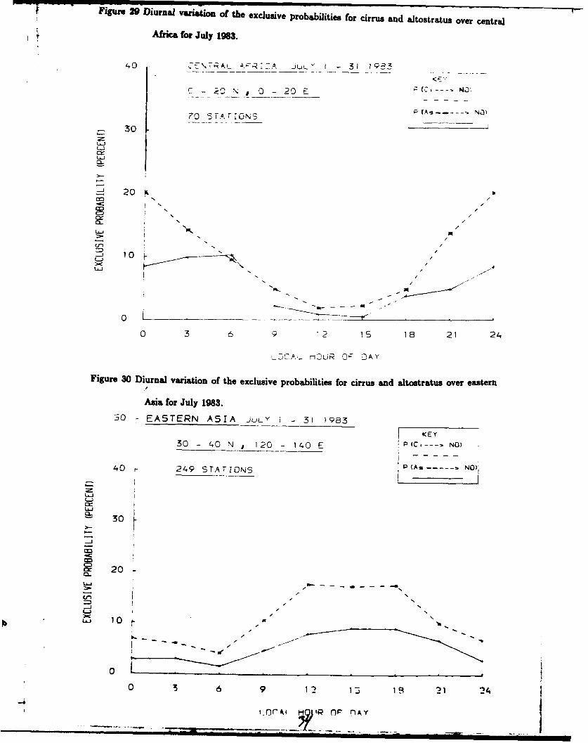
Figure 29 Diurnal variation of the exclusive probabilities for cirrus and altostratus over central

Africa for July 1983.

40 A ,A j "I - 31 19 33

C - 20 N 0 - 20 E NO

70 S TAr ON3

30 -

L.

L.J

-0 1

/ 7 , °

L

0 3 6 9 !2 15 16 21 24

Figure 30 Diurnal variation of the exclusive probabilities for cirrus and altostratus over eastern

Asia for July 1983.

30 EASTERN ASIA JULY I - 3' )983

KEY30 - 40 N s 120 - 140 E P(C-. NO)

SP (As - - NO):I40 249 STATIONS ... N

cx I

30m

-

C" 20

0~

0 3 6 9 12 15 1. 21 "24I. in o

for January 1985.

* SCANDINAvIA - _ANuA.R- '

60 - 70 N 10 - 30 -"

P 'As - N0

j5S STAT IoN5

30U~jC.)CX

- 20

tmo

--J 10

azi

0.

0 3 6 9 12 15 18 21 24

L.DCA- rOL;R 0P DAY

Figure 32 Diurnal variation of the exclusive probabilities for cirrus and altostratus over the central

U.S.A for January 1985.

00 -CENTRAL J.S.A JANUARY I - 31 1985

; KEY

90 , 30 1-A IN40 N 1 90 11I0 W P(C-- .. . NO)N)

-- -

70

60

LCCLiURQ A

0P (A 6- 9i2

- H,,,

L.J 70,"

40 ,- 6--2 S 1 2

La..i I -' l l I

Figure 33 Diurnal variation of the exclusive probabilities for cirrus and altostratus over central Africa for January 19"

I0 CENTRAL AFr-:.CA ,A\uAQV 1 31 X ----

90 - O0 - 20 N , - 20 F

P!A 9 ... NO)

80 - 70 STAr ONS

70

- 60 r -..

0r 40

30 -

.20

10 i-

0

0 3 6 9 12 15 18 21 24

LOCAL -iOu O" DAY

'igure 34 Diurnal variation of the exclusive probabilities for cirrus and altostratus over eastern Asia for January 1985

20 - EASTERN ASIA JANUARY I - 31 1985

30 40 N 120 1 40 E P(C. > NO)

40 r 249 STAr [ON? P (As ..... NO),

-. L J

C-

306

CrI

L-1

L*J 10

0

0 3 6 9 12 15 1 21 2 4

LOCAL HOUR OF DAY

36

cirrus or altoetratus by itself. Over the central U.S. much of the peak at 6 am is gained during

darkness hours and is therefore probably not due to observer error. Over eastern Asia, however, in

a region likely to experience convective cloud from the summer monsoon, the broad peak for cirrus

is conspicuous although the rise it represents is only of the order of 10%. The data from January

are of limited value although an interesting feature is how the shape of the curves over Scandinavia

resembles the corresponding frequency curves. Here, however, the peaks are considerably smaller

and consequently less significant.

Recent developments in satellite cloud retrieval permitted cirrus to be accurately detected

during darkness (Inoue, 1985; Saunders, 1986; Saunders and Kriebel, 1987) from polar orbiting ra-

diance data. Further insight into the impact of nocturnal bias may be possible from satellite/surface

comparisons using these new algorithms.

2.6 The Use of Contingency Probabilities for Situations of Partial Undereast Bias

The term partial undercast bias (PUB) (Hahn et al., 1984; Warren et al., 1986) refers to a

situation when an observer fails to detect the presence of middle or upper level clouds because they

are obscured by a (non-overcast) lower layer and do not overlap into the clear region of the sky

(Figure 35). The likelihood of incurring PUB increases as the amount of the non-overcast obscuring

layer increases and such an occurrence repeated many times leads to a systematic underestimate

in the frequency of occurrence of middle and upper clouds. This, in turn, is likely to reduce the

quality of surface-based cloud climatologies.

The use of contingency probabilities in such cases has been suggested as a means of avoiding

PUB in surface retrievals where they would be employed by the observer whenever PUB was

suspected. Specifically, two types of probability have been defined. The first defines the likelihood

that given the presence of a lower cloud L upper cloud U is also present and is denoted by P(L=*U).

A second type of probability is simply the opposite of P(L=*U) termed P(Uf:L). The latter type is

men as a possible means of using surface observations to aid satellite retrievals in multilayered cloud

37

C>=

7777/7777777 11711111177177

Schmaic llstrtin f Prtal ndrcat ia

Fig re 5 Ilusraionof he ~yparialundrest iasoccrs

38/... ..... .... ...... .....

scenes where the satellite was only detecting the upper cloud U. Use of P(U*L) could improve

the retrieval in the long term - although it would sometimes falsely predict the presence of some

types.

If contingency probabilities were to be used operationally, the observer must know how the

values vary over the whole range of lower cloud amounts, i.e. whether he should use the same value

for 2 oktas of L as he would for 7 oktas. The values of P(L*:U) computed by Hahn et cl. (1982,

1984) were constructed on the assumption that the value of P(L=*U) is invariant over the whole

range of amounts of L including when L is overcast. They tested the assumption on data from the

northern hemisphere for the months of March, April and May 1971, plotting P(L=*U) as a function

of the amount of L when L was not overcast. Their findings are shown in Figures 36 and 37. In

Figure 36 'As' denotes the cloud types altostratus and altocumulus whilst 'Ci' in Figure 37 denotes

cirrus, cirrostratus and cirrocumulus and in both diagrams 'St' denotes the cloud types stratus and

stratocumulus. The assumption is relevant only for U= altostratus or cirrus explaining why the

particular combinations of L and U were used. No analysis was carried out for the combination

L= altoetratus, U= cirrus because the observer can only gauge amounts of altostratus correctly

when there are no obscuring lower clouds and such cases might be unrepresentative of the whole

set of altostratus observations. In both diagrams there is no strong indications that the value of

P(L=*U) changes greatly over the range of amounts of L and the values corresponding to 6 or

7 oktas differ only by a few percent from the mean for 1-7 oktas. Hahn, Warren and London

concluded from these results that, overall, their assumption about P(L=U) could be deemed valid

and was subsequently taken to be so.

The global data for January 1985 and July 1983 provided the opportunity to check the be-

haviour of P(L-*U) over different areas of the world including the southern hemisphere. Areas

of Australasia, eastern Asia, Africa and Scandinavia (Figure 38) were selected, the United States

39

I , n ,IN ll ill IU

6040

50 30 60.

040- 40 0 - 40

4 20r 2

AMUT fS , HH f-K OE

Figure ~ ~ ~ ~ ~ I. 30Vraino otnec rbblt fAsA o ie mut fS/ itga

Q b a s s ow he ela ive nu m er o ob erv tio s c ntrb ut ng t ea h p int D a h ed lin

inicte manvaueofal te bsrvtinscrbtn tote ont.Dtafoth nrter hmiphre Mrc, prlMa, 97 (ro Hhnetat, 98)

igure 36 Variation of contingency probability of Ai/s/Ac for given amounts of St/Sc. Histogram

CL3 bmr show the relative number of observations contributing to each point. Dashed line

indicates mean value of all the observations contributing to the 4 points. Data from

the northern hemisphere, Mach, April, May, 1971 (From Hahn et 0., 1982).

not included because the majority of the reports there were of the airways category which de-

scribed cloud cover as either clear, broken, scattered or overcast rather than with a specific okta

value. For each region the contingency probability P(L*-U) was calculated for amounts of L in

the range 1 to 7 oktas. The method involves dividing the number of occasions on which L and

U were men together by the number of times L was observed and the level appropriate to U

reported (either with or without U). The results for L= stratus/stratocumulus and U= altocumu-

lus/altostratus are shown in Figures 39 to 46 and those where L= stratus/stratocumulus and U=

cirrus/cirrostratus/cirrocumulus are in Figures 47 to 54. Each diagram contains 2 vertical axes -

the left-hand axis relating to the contingency probability, the right-hand axis being a percentage

scale for the bar histogram.

2.7 Resust

i) L = St/Sc, U = Ac/As

The overall trend in both January and July is for P(L=oU) to decrease with increasing U but

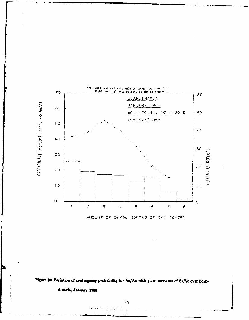
there is considerable variability between the countries. The largest decrease occurs over Scandi-

navia, approximately 35% in January and 45% in July for amounts of St/Sc ranging from 3 to

7 oktas. The horizontal bars in Figure 40 indicate the mean value of P(L=*U) over 1-7 oktas

(upper bar) and the mean value over 6-7 oktas (lower bar), the difference between them amounting

to almost 25% cloud amount (absolute). Over eastern Asia the decrease, although steady is less

pronounced, the bars in Figure 41 being separated by only 10%. The assumption that P(L*U) is

constant for all amounts of U could not be said to hold over these areas. A similar conclusion can

be drawn from the Asian data in July where the decrease of P(L=oU) is almost linear. Here too

the chance of observing altostratus or altocumulus appears to decrease with increasing St/Sc. In

other words, in all the above cases the risk of PUB is somewhat lower for more lower level cloud,

in conflict with the assertions of Hahn, Warren and London.

4'1

A

'o c 0 CN S, ' 01o i 0 11 0 L Cn Ul C' 0 0

LII0

CA

10

LA

I 42

Key: Left vertical axis relates to dotted line plotRight vertical axis relates to the histogram

SCANDINAVIAcr

JANUARY iQ;560

60- 70 N . 10-30E 50A

A,, 155 .5AT EONS

cr 5040

LLI

'30 c

-.-.

_ 2323

'3 i0 C

2 3 " 6 7 0

AMOUNT OF St/S - Q.KTAS OF SKY CJVER)

Figure 39 Variation of contingency probability for As/Ac with given amounts of St/Sc over Scan.

dinsvia, January 1965. 4

IF4sre 40 varnasuu uL wucsenucy Prubabdity tor As/Ac with given amounts ol St/bc over 5canlwln&vLa, July L9M.

Rev: Left vertical Ixis r elates to dotted linle plot

Right vertical axis relates t, the histogram

36D

-~ JULY IQB57. 33 0_ -D-- - " -- "" , 0 - 70 NJ._O 50E'50$

I /

69 A 148 -TAT[ONS

to

U-W 4,0 30 v-,

LUX>- C

z;3 30 C

M-. 20 'C-:

rLx

SC12 2

0 0

2 36 7 83

AMO1UNT ODF 3-t/Sc (C'(-TA' -,F SKY J1FVRI

Figure 41 Variation of contingency probability for As/Ac with given amounts of St/Sc over eastern

Asia, January 1985.

Key Left vertical axis relates to dotted line plot

6 3 Right vertical a~xis relates to the historam

EASTERN ASIA

" 9-0 JANUARY i985

30 -40 N . 120- 140E 50

4.0 263 STATTONS

34

20 4300

ZA

co 20 L-

00, 0 L]-x.

Lx

2 3 4 6 8

AMOUN T OP St/Sc 'OKTAS Or SKY COVER)14

Right vertIC31 a relates tc the histogram

6C --- _ _ __ _ _ _ _ __ _ _ _ _ __ -0_ _EASTERN ASIA

CS JdJy 19E3

"30 40 N Z40 E 5C40 249 SrArION-:

3040

20 1.2

Lj

0. - 3 0 c

'D

M 0C 20 cC--

C-

2 3 " 9 6 7

AMOUNT OF St/Sc (OKTA,C OF SKv CJVER)

Figure 42 Variation of contingency probability for As/Ac with given amounts of St/Sc over eastern Asia, July 1983.

Figure 43 Variation of contingency probability for An/Ac with given amounts of St/Sc over central Africa, January 19Kev: Left vertlcal aX: reiateb to dotted iine p:ot

Right vertical ixs relateps to the histogram

60CENTA'_ kFPIZ1CA

" ' JA.NL ARyi B5

0 - 20 N 0 -20 E 50

A ? tO SAT'JNS

30 S ,

-C-) LiL

30 ! !

C=) 20 2

00

I C-

2 1 0

2 5 " 6 7

A .MOUN OF St /c 'JKTAS OF 9Kv COVER'

1.5

Contrasting results were obtained for the central African data. In January (Figure 43), the

value of P(L=*U) falls off by 25% in progressing from 4 to 7 oktas St/Sc but the July trace (Figure

44) is almost horizontal until the considerable decrease at 7 oktas. As the number of report. leas

than 7 oktas constitutes 75% of the total, the use of a single mean value of P(L=*U) over the whole

range of amounts of L would give only slightly higher frequencies of As/Ac when 7 or 8 oktas St/Sc

were present.

Only over Australasia (Figures 45 and 46) do the results bear close resemblance to those

obtained by Hahn et al. An interesting feature of all the plots is the small percentage of reports

associated with the lower cloud overcasts (<10% in each case) compared to greater than 40% found

by Hahn et al.

ii) L = St/Sc, U = Ci/Cs/OC

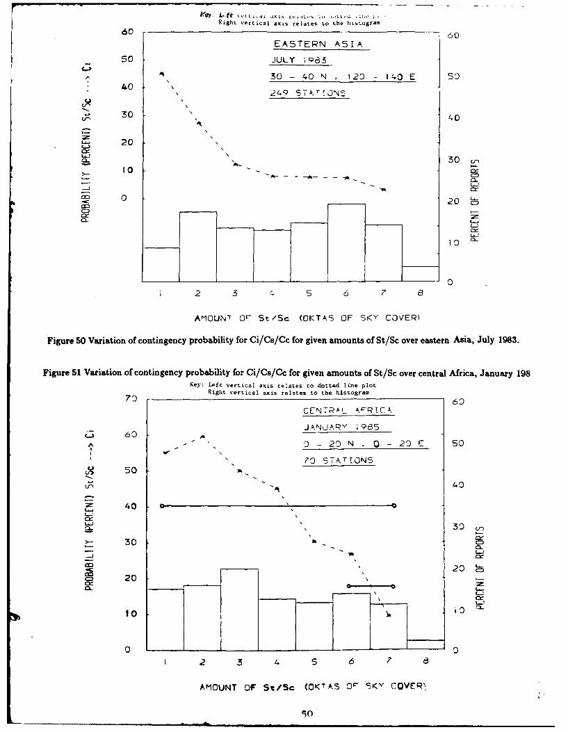
Similar trends in contingency probability were obtained, particularly over Scandinavia where

the assumption is shown to be invalid for the data over both months. (Figures 47 and 48). Over

Asia and Australasia (Figures 49, 50, 53 and 54) the trend is rather steadier as the amount of St/Sc

is increased and the mean values do not differ from the values at 6 or 7 oktas by more than 10%.

The contrast in the African data between January and July is much reduced as is evident from the

horizontal bars. Overall, it appears that the tendency for high cloud to be present is greater when

there is less than 4 oktas of stratus or stratocumulus.

Although the results presented here do not permit general conclusions to be drawn, they show

some disagreement from those of Hahn et al. Variation around the globe is evident. The frequency

with which different cloud types occur simultaneously giving rise to PUB should help to promote

the idea of contingency probabilities but the results presented heze i) cast doubt on the choice of

a single value for P(L=*U) for given types of L and U and all amounts of L and ii) suggest that

PUB is perhaps not so common for higher amounts of L as might have been thought. The concept

of contingency probabilities is recent and their future role seems likely to be in the construction of

46\

A'

Key: Left vertical axis relates to dotted ilne plotRight vertical axis relates to the histogram

60 ._ fT . "5"'

JULY 1983 I

-- O 40 S 120 IO -

47 5- T[2T 7

Ln

30

L.J00 -

>--

__jn_* 20-

- 0 0-

2 4 -

A''-_.,. O S-t/Sc Ci E 0R

Figure 46 Variation of contingency probability for As/Ac with given amounts of St/Sc over Australasia, July 1983.

Key: Left vertical axis relates to dotted line plot

40 Right vertical axis relates to the histogram 60-:-A .N2 r \iA.V :A

JANUARY iQ5e

60 -70 N .10 - so

30 i5 -3TrrN

'-L

100 - II

-J I 0., "

I 2 3 6 7 a

AM'OUNT OF 57J/5C (J <Tk, S OF SK"' rOVE'S Vr i

Imut o20S oe cndnva 3susy195Fim14 Vrion. o10nilnypoaiiy o iC/cfrgv

--- il I m l~ m I l i a I, I - ,

Key: Left vertical axis rei-ates to dotted line plot

Right vertical axis relates to the histogram

100 F '-ENTPAL OFRICALb Y I9I

JUL-Y 1983

ao 0 20 N C-( 2D

6 4 c; ArT j N

70J aa 4

U.

* 60 -

"' 50 30

CDf

40 c-

C 20Co 30

20 A1-~

10

0 0

1 2 3 " 5 6 7 3

A'MOUNT 3F St/5c (OKTAS 3F SKY COVERI

Figure 44 Variation of contingency probability for As/Ac with given amounts of St/Sc over central Africa, July 1983.

'igure 45 Variation of contingency probability for As/Ac with given amounts of St/Sc over Australasia, January 1985.Key: Left vertical axis relates to dotted line plot

Right vertical axis relates to the histogram

... . ....... ... . . 6 0SA'JS TR ALAS A

JANUARY I 95

A -- 30 - 0 5 , 120 - 180 E 50

.6 STATIONS

, , 40

30. /

20 .30 U,

10 1r

C ~20 C"

0

"-- L 10

2 3 4 5 6 a

AMOUNT OF St/$c (OKTAS OF SKY COvEP'

Its$

ac i. %ert i ;, ax, tt 'ite*S to dotted line plotRight vertical dxis relates to the histogram

6.)

3CAND r NAV [A

I cY - ON.50- O 70 N 10 3"3 E_ =

141 57AT rONS

4S

30•*I 4

330

-- . L-J

cm 20 20

ii 0

1 2 3 7

,MOU3NT Df- ST/SC ,OKTAS OF SKY COVER'

Figure 48 Variation of contingency probability for Ci/Cs/Cc for given amounts of St/Sc over Scandinavia, July 1983.

Key: Left vertical axis relates to dotted line plot

Right vertical axis relates to the histogram

50 60

EASTERN ASIA

JANUARY iQ85

30 -40 N . 120- i40 50

263 STATIONS30

40

20&-j

C1 20 ULIL

2 3 4306 7

20 LZ

cc-

AMODNT 00 St/Sc tOKTAS Qr SK Y CIJER

Figure 49 Variation of contingency probability for C i/CuI/Cc for given amounts of St/Sc over eastern AUsia Jaau&7 1985l.L

CXI~ I I I IIIIIII

Vey i.ft

Right vertical axis relates to the histogram

60 60

EASTERN ASIA

50 JULY iQ83

40 30 -40 N , 120 -140E 5410 ", ~249 S7T",r TJNS

30

V0 200

,-, 30

10 10'

2 3 4 5 6 7 a

AMOUNT 0 St/Sc (OKYAS OF SK Y COVER)

Figure 50 Variation of contingency probability for Ci/Os/Oc for given amounts of St/Sc over eastern Asia, July 1983.

Figure 51 Variation of contingency probability for Ci/Cs/Cc for given amounts of St/Sc over central Africa, January 198Key: Left Vertical axis relates to dotted line plot

Right vertical axis relates to the histogram70 6D

CENTRAL AR'TC.,

JANUA'Ry j 985Li] 60A

^-" D -20 N O- 20E '50

I " ~~70 STT.',r[iO-NS50

40

2- 30 "5 6AMUN 407 StS SSOFSYCVR

c---

30

Fgr20 o ,

Ke: L10 1JAiU .,.85

0 _________~1 0

I 2 3 4 5 6 7 3

AMOUNT OF S20Sc (OKNAS 0 " 9v CVE 50

70 STTTON

V 50

Figure 52 Variation of contingency Probability for CICS/Cc for iven.........f.St.... o eCentral Africa, July -98 .: Left vertical axis relates to dotted line plot given amout/ c 0.,,Right vertical axis relates to the histogram

80CEN TRAL A, ;7 Q. CA

70 JULv 1983

0 -20 N 2060

84 STAT IONS

50

40

Cr 30

30 , .I-3

20 20 _

10u-,

100

01 2 3 5 8

AMOUNT 0 St/Sc (OKTAS OF SKY COVER)

'igure 53 Variation of contingency probability for Ci/Cs/Cc for given amounts of St/Sc over Australasia, January 1985.

Key: Left vertical axis relates to dotted line plotRight vertical axis relates to the histogram

60 60

AUSTRkALA$ [ A

JANUARY 198550

30 - 40 S , 120 -180 E 5o1 .6 STATIONS

4 0

40

S ,30 30

- 20

al- 0 C2 0 i

00 (1C:) 10

1 2 3 4 6 7 8

AMOUNT OF St/Sc (OKTAS OF SKY COVER)

Key: Left vertical axis relates to dotted line plot

Right vertical axis relates to the histogram

72/' L Au 2IT;A "L' "

JULY - z

3 60 - 40 S, 120 -180 5

i' - 47 STAT IONS

4-D-

3030

L J

< I - -D I 1

" 2

0 .. . ..-; 0 u

. . . . .. : I! 1 0 C3-

" J 0

1 2 3 6 8

A1M0J T IR : " '; -XK'T A.c 0F 5-3 : Y COVER)

Figure 54 Variation of contingency probability for Ci/Cs/Cc for given amounts of St/Sc over Australasia, July 1983.

1 OOC AUSTRALAS I A

JANUARY I - 31 1985

900 30 - 40 N 140 - 180 E

35 STATIONS

8oo

700

CD

600.-.I

.-J 5QOf Soo

t.----

_ 1

400

C= 300 IIJ

200 III I I

100 II I

I g I

0 2 3 4 7 6 8

TOTAL CLOUD AMOUNT (OKTAS)

52 .

P'",rP 'So TntRl elniid RMnllnt frven11#nrv hietnae-rvn fhr Aiiatrstm.am 1fl9c

surface-based cloud climatologies for climate studies, especially modelling. At present attention is

focussed primarily upon satellite-derived climatologies and hence the potential role of the opposite

probability, viz. P(U=L), should be further investigated.

2.8 1 and 7 okta bia*

The WMO procedure for reporting total cloud amount assigns special rules concerning values

of I and 7 oktas. It requires that the observer report 1 okta of cloud even if the amount present

is less than half an okta, i.e. every cloud present must be recorded. At the other end of the scale

small gaps in a cloud sheet, even if they amount to less than half an okta or are only suspected to

be present, should be recorded as 7 oktas rather than 8. These rules are not always strictly adhered

to and observers around the world may tend to round off their estimate to the nearest okta, often

in an attempt to record the more realistic value. Very small clouds or gaps are easily visualised, e.g.

a thin streak of cirrus in an otherwise cloudless sky, remnants of daytime cumulus at dusk, isolated

cumuli and the small holes characteristic of stratocumulus decks. Assuming that observers stick to

the accepted procedure small biases in the total cloud amount may arise if a location experiences

frequent cases of either very small clouds or small gaps. If both cases occur often the overestimation

of cloud amount by using I okta counters the underestimate of cloud amount caused by using 7

oktas and any bias is considerably reduced. Remembering that an okta is 12.5% cloud amount

serves to highlight the observer's choice of okta value.

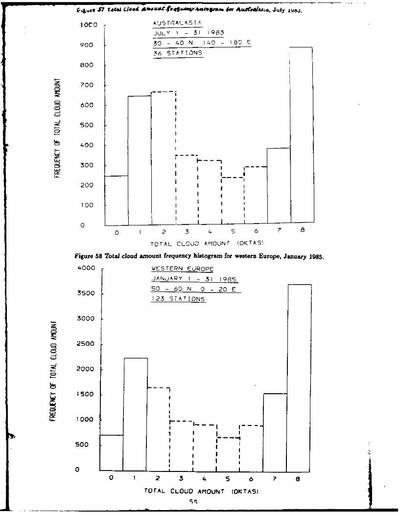
As a brief exercise aimed at checking for cases where there is a strong suggestion that I or

7 okta bias might prevail, areas of Australasia, Europe, India and South America were chosen

(Figure 55) and the frequency of occurrence of total cloud amounts plotted as a histogram for

all the stations within each area. The histograms were examined for incidences of very high (or

very low) relative frequency of 1:0 oktas and 7:8 oktas that suggest under or overestimation of

the monthly mean cloud amount due to the (correct) application of the observing rules. Then

histograms are shown in Figures 56 to 61 and show 3 interesting examples. The July histogram for

53

III|1II !i

ILJ

0

OD

0

u,

wu0

0fn

0

ILAJ

o.

0

0

0oLei O-

z z zz z I in

LP 0 n 0 U0 ul 0 Lrl LnW) - 10

Ok 10o

JAur 7 fetaS £1d 4SMtfSidnVde1*.4"frAi~ia51,, July jboj.

I CO A'J5 Ts AL AS A

JULY I - 31 1 Q83

900 30-40 N 1 40 - ,80

36 STAT!ONS

800

700C=)j_ '600

500

C 400

C=3 300

"I -200 1 1 1

0I I

100/I10 |_ _ _ I I i

0 1 2 3 4 - 6 7 8

TOTAL CLOUD AMOUNT (OKTAS)

Figure 58 Total cloud amount frequency histogram for western Europe, January 1985.

4000 WESTERN EUROPE

JANUARY I - 31 1985

3500 50 -60 N 0 - 20 E

123 STATIONS

-- 3000

m 2500

-DLj

2000

! i11500

LA. 1000I I-

1 !

500 I I I

I I0 _ _I I I _ _ _

0 1 2 3 4 5 6 7 8

TOTAL CLOUD AMOUNT (OKTAS)

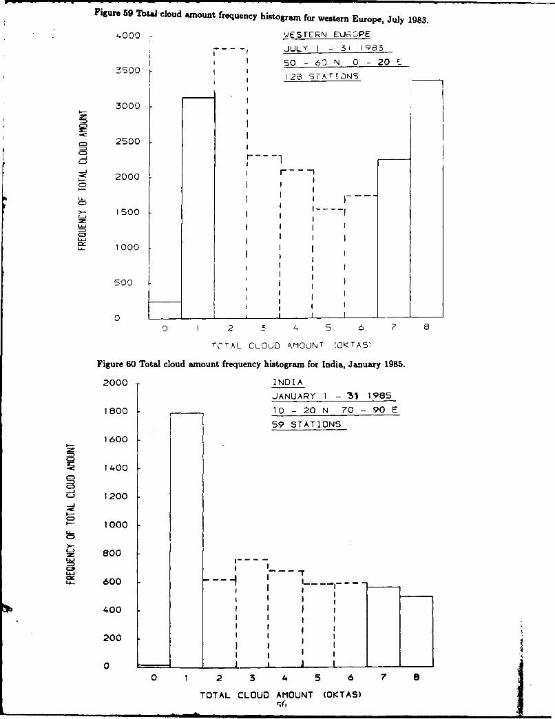
Figure 59 Total cloud amount frequency hitogram for western Europe, July 1983.

4000 WESTERN EURF<PEJULY I - 31 1983

50 60 N 0 20 E

3 128 STAT[ONS

3000

_m 2500= I

C=1

2- 0001500

2 1000 IN IJ I

5600

I

0I_ _ II . . . .15002 5 I 5.. 6

24000 N

I-

1400

6j 1200

CD

1- 1000U-

C-D

Bo0

I-

LAJ

W -TLa.. 600--1------

O I I I

400 I

200 I

100

II6 0 - -- - I . . . . . .

0 1 2 3 4 5 6 7 8

TOTAL CLOUD AMOUNT (OKTAS)I_

a.a)

00 0

0bO N 0

T- < D

0 z F

c~oi<-F'I 0

0

o 0 0 0 0 00 0 0 0 0 0 0 0 0 0o DN 4 N 0 0 0 0 0

co 110- N 0

INflOWV Ofll lYioi AO ONNfORA

57

western Europe (Figure 59) shows case of clear sky comprising about 2% of the total reports with

a ratio of incidences of 1:0 oktas of the order of 15:1. The frequency of clear sky is well below the

mean long-term value over the area for June, July and August 1971-1980 of 10% quoted in Hahn

et al. (1984) and it was by no means an abnormally cloudy month over the region.

Sharp peaks in the histograms for I okta were also found over India and South America for

January 1985 with less than 1% of the total number of reports in each case showing 0 oktas. The

corresponding climatological frequencies quoted in Hahn et al. are many times higher and since in

both cases the frequency of 7 and 8 oktas is very similar (not ruling out 7 okta bias but suggesting

that no strong preference for 7 oktas exists) it seems likely that the reporting practice is in these two

examples (particularly over India) leading to an overestimate in the mean monthly cloud amount.

With only two months of data at our disposal it is not possible to determine whether the above were

isolated cases or whether this bias is more extensive. It ic generally assumed that the observing

procedure is self-compensating in respect of this type of bias and so little, if anything, seems to

have been done to correct for it in the past. Although it may be of limited importance compared

to the other biases discussed here, the examples above indicate it worthy of further consideration.

3. Global evaluation of surface cloud observations

3.1 Data

The data set is identical to that used in the bias investigation, the source and format of which

was outlined in Section 2.2. Data used for climatological purposes should be as representative of

an area (or station) as possible. Therefore despite the problem of likely attendant bias, nighttime

observations were included in the analyses and given the same weighting as daytime reports. No

substantial diurnal sampling bias was discovered although it is known that a few stations do not

report at night. The numbers of reports from land stations considerably outweighed the numbers

58

• ,I II I I I •• • III I I I

received from ships, partly due to the fewer stations at sea and partly because clouds are recorded

only at 6-hourly intervals from ships (0, 6, 12 and 18 GMT) whilst synoptic reports on land are

required every 3 hours (0, 3, 6, 9, 12, 15, 18 and 21 GMT). All reports were coded according to

the WMO cloud classification (WMO, 1984).

3.2 Biases ,itain the observations

Surface cloud observations decrease somewhat in value when the clouds assume complex layered

arrangements and their correct reporting becomes subject to varying degrees of bias, particularly

during the hours of darkness. Problems of nighttime detection and those associated with "partial

undercast" situations are discussed in Section 2, as are the slight biases resulting from the accepted

definitions of 1 or 7 oktas cloud amount. In addition to these the observer is unable to detect

middle or upper level clouds in the presence of an obscuring overcast. This layer obscuration bias

can result in systematic underestimates of cirrus in many cases. Over the oceans observations made

from transient ships may be affected by the use of inexperienced or untrained observers who may

fail to record the presence of a particular cloud type or misinterpret other types. Certain ships are

likely to alter course slightly if it permits them to bypass severe weather, thus introducing what is

termed "fair-weather" bias. Bunker (1976) and Quayle (1980) compared observations from weather

ships with those from passing vessels to assess the impact of these two biases whilst Hahn et aL

(1982) analysed the data from Quayle to compare cloud amount estimates, finding that there was

very little difference between estimates from stationary weatherships and passing ships in close

proximity.

The need to avoid contamination of reports by bias prompted Warren et at. (1986) to use

only daytime observations of cirrus, altostratus and altocumulus for constructing their global maps

of frequency of occurrence of these cloud types. As increasing amounts of low and middle cloud

increase the risk of incurring partial undercast bias, reports of upper cloud in multilayered situations

were restricted by Warren et W*. to those with no more than 6 oktas of lower cloud present.

59

Tabb 0 Some.. of Dims witbi Surace Obiwaeiuno

i) Wfghktdciom him

ii) Partialumdecau hia

SO) 1, 7 &tabin

iv) fair-weathm barn

V) Obmwi bin

Ai Layer obscuratio h

600

Surface cloud retrievals are known to "overestimate' cloud amount systematically compared to

satellite data (Godshall, 1971; Hoyt, 1977). The skycover measured by an observer on the ground

may exceed the earthcover detected by the satellite when the clouds have significant vertical as well

as horizontal dimensions. A relationship between the two quantities has been proposed by Malick

et al. (1979) on the basis of the analysis of a large number of all-sky photographs. It should also

be noted that the sides of vertically developed clouds bias (upwards) any satellite-derived estimate

of cloud amount when look angles are other than zero.

Eliminating reports in which bias is suspected represents the easiest method of removing the

effects due to bias since at present they have not been quantified. However, such a policy war not

adopted here. A list of the principal biases is given in Table 6.

3.3 Analysis Procedure

i) Extraction of Required Information

The first requirement for any report, either from land or ocean, to be used was that its source,

i.e. latitude and longitude both fell within sensible bounds. All reports originating from bogus

locations were rejected from the analysis to avoid mislocation. A complete report comprised a

value of total cloud amount in oktas, 9 being used to indicate obscuration of the sky by either

mist/fog or falling precipitation; a number in the range 0-9 describing the type of low, middle and

high cloud present according to the WMO classification as given in Tables 1-3 with 255 denoting

obscuration of the appropriate layer; a value for low cloud amount in oktas (or middle level amount

in the absence of low cloud) and a subsequent report of the type, level and amount of the "first

reported layer". It was difficult to identify any definite trend as to which layer the first reported

layer referred. If there were additional layers to report these were detailed in the "additional data

section' of each report with the type and amount supplied for each additional layer. In some cases

difficulties aroe when it was discovered that all the relevant data were located in the additional data

61

section after the main section of the report had indicated no information available. As a precaution

a contingency operation was used to make sure that all available information was extracted from

each report.

ii) Cloud Type Categories

Tables 1 to 3 are derived from the WMO manual on codes (WMO, 1984) and define the 27

cloud types of the synoptic code that are known to occur. All these classifications are well illustrated

in the most recent WMO cloud atlas (WMO, 1987). Nine separate categories are defined for low,

middle and high clouds; however, a more simplified grouping of cloud types was required for the

purpose of global evaluation. The 27 categories were merged into six following the method of Hahn

et al. (1982). Table 7 defines the six merged groupings and the WMO codes associated with

each grouping. The 27 original categories do not always define specific occurrences of individual

types, particularly for middle and low clouds. For example low cloud category 9 (CL = 9) denotes

principally cumulonimbus whilst permitting the possible presence of cumulus, stratocumulus and

stratus. In such cases it was decided that the principal cloud type defined in a code would be

exclusive to that code number. This policy may have been responsible for the introduction of slight

biases for certain cloud types. As there was no code number defined exclusively for nimbostratus

the requirement for its presence in the codes CM = 2 and 7, was that the station was experiencing

precipitation at the time. The present weather code was checked in such case. It was also decided

that if CL = I was reported together with precipitation, then nimbostratus was present too. Cases

of clear sky were defined by zero sky cover or, if unavailable, by the absence of clouds from each of

the three reporting levels.

iii) Cloud Amounts

Total cloud amount represents the skycover as estimated by the observer in oktas. Whenever

a value of 9 was encountered the presnt weather code was checked for fog or precipitation events.

It was decided that in either case the use of 8 oktas would be representative despite the small

62

Table 7 Merged Cloud Types

Cloud types referred WMO Observer Codes

to Aere assigned to each type

1. Cirrus (Ci)/Cirrostratus(Cs)/ CH 1-9Cirrocumulus(Cc)

2. Altostratus(As)/Altocumulus(Ac) CM 1,3,4,5,6,8,9and Cm 2,7 if no precipitation

3. Nimbostratus (Na) CM 2,7 if precipitationand CL 7 if precipitation

4. Cumulus (Cu) CL 1,25. Cumulonimbus (Cb) CL 3,96. Stratus(St)/Stratocumulus(Sc) CL 4,5,6,8

and CL 7 if no precipitation

Notation used in text and

figures is, group 1 is hereafter referred to as Ci/Cs/Cc

group 2 is hereafter referred to as As/Ac

group 3 is hereafter referred to as Nsgroup 4 is hereafter referred to as Cu

group 5 is hereafter referred to as Cbgroup 6 is hereafter referred to as St/Sc

63 1

number of occasions in which precipitation does not descend from an overcast sky for example, at

the end of a shower when skies are clearing. Values of '9' were discarded if the present weather

code failed to indicate fog or precipitation. The code parameter NH referred to the amount of low

cloud present AC = 1-9) or middle cloud (Cm = 1-9) if no low cloud was recorded. Information

relating to the "first reported layer" often gave the amount of cloud in the same level as for NH

making it redundant.

The maps depicting the distribution of cloud amount were constructed only from reports

where the cloud was present. They, therefore, depict the average "amount when present" and are

representative of exactly what the observer sees (in terms of amount in each layer), i.e. for separate

observations in the presence of two layers, the random overlap equation was not adopted. The

time-averaged cloud amount is defined as the product of the frequency of occurrence of cloud at

a particular level and the mean amount when present for the same cloud. These maps have not

yet been constructed for the data concerned but may serve a useful purpose in comparison with

time-averaged products from ISCOP (Table 1, Rossow et at, 1985).

iv) Frequency of Occurrence of Cloud Types

The frequency of occurrence of a cloud type is defined as the number of times the cloud type

is observed divided by the number of occasions information about that cloud level is received, i.e.

the code for the level lies in the range 0-9 or is supplied in the additional data section. As expected

the number of reports supplying information about the middle and upper levels is rather less than

the number contributing to the low cloud statistics. The frequency of clear sky was defined as the

total number of occasions when either the skycover was zero or each level was devoid of clouds,

divided by the times when information on all three levels was available.

The maps for low level cloud should be representative of reality but figures computed for middle

and upper level clouds are affected (to an unknown degree) by partial undercast bias, causing a

systematic underestimation in the frequencies of both cirriform (Ci, Cs, Cc) and altiform. (As, Ac)

6 4'

clouds. The contingency probabilities (part vi) provide a measure of the likelihood of middle or

upper cloud being present when partial undercast bias is suspected. As the future role of the maps,

if any, would lie in comparison with satellite retrievals rather than in climate modelling studies, the

frequencies have not been modified to include biases and the contingency probabilities are evaluated

separately.

v) Exclusive Probability

The exclusive probability of occurrence refers to the chance of an observer detecting an in-

dividual cloud type by itself. It was defined here as the number of occasions a particular type

was reported alone divided by the number of times information concerning all three cloud levels

was given in a report. Individual types occurring with regularity by themselves, especially cirrus,

indicate useful testing grounds for algorithms aiming to retrieve a particular type (cf. Starr, 1987).

vi) Contingency Probabilities

The concept of contingency probabilities as applied to the co-occurrence of cloud types was

introduced by Hahn et at. (1982, 1984). Examples of contingency probabilities of the type

P(Lower=*Upper) are presented here for various combinations of lower and upper cloud (Table 8).

The idea was introduced as a means of avoiding unnecessary levels of bias in surface observations.

If, for example, an observer suspected the presence of cirrus cloud but could not detect any through

a small gap in a stratocumulus layer, the contingency probability P(Sc =: Ci) would indicate the

(long term) likelihood of cirrus being present. The values computed for these maps assume that the

likelihood of the upper cloud being there is the same when it is visible to the observeras when it is

invisible to the observer due to the lower cloud being overcast. Whether this assumption conforms

to reality is discussed in Section 2.

The probabilities are computed as follows. The number of occasions on which both lower and

upper cloud types were present is divided by the number of times the lower cloud is present and

information about the upper level was available, i.e. it was not obscured from view. No probability

65

Table e Combinations of Lower (L) and Upper (U) Cloud Type Used In

Contingency Probability Determination P(L=*U)

L U

1. Cu Ci/Cs/Cc

2. Cb Ci/Cs/Cc

3. N9 Ci/Cs/Cc

4. As/Ac Ci/Cs/Cc

5. St/Sc Ci/Cs/Cc

6. Cu As/Ac

7. Cb As/Ac

8. St/Sc As/Ac

66

was computed if a grid square contained less than 20 occasions on which both upper and lower

clouds were observed.

3.4 Map Format

The maps are divided into two sections, those for land and those over

the ocean. There were approximately half the number of ocean stations

(ships) as there were land stations, in both months (- 5000 compared to .- 9MO). The land data

are mapped at a resolution of 50 x 50 (ISCOP data are to be mapped at a resolution of 2.50 x 2.5*)

for the area of the globe lying between 6 0 N and 6005. To maintain an approximately equal area

within each grid square the resolution was increased to 100 x 100 poleward of 60*N and 600S,

although it is recognised that this is by no means a perfect remedy to the problem of the Earth's

curvature at higher latitudes. The oceanic data were plotted at a resolution of 100 x 200 except

for cloud amounts which were mapped at 100 x 100. The world coastline has been superimposed

on to the ocean maps but is absent from the land maps although in most cases the outline of the

continents is recognisable.

The numbers have been plotted at the geographical centre of each grid square and in certain

cases may overlap onto neighbouring land (or ocean). In such situations the number will be repre-

sentative only of the land (or ocean) fraction contributing to the grid square. The ocean data except

for the distribution of observations are given as percentages but in order to avoid numbers running

into one another over the higher-resolution grid squares on land, the percentages are represented as

single integers representing 10 percent increments, even though this process is rather downgrading

the information. Maps showing the density of observations are presented in tens over the ocean and

in hundreds over land. A plus sign indicates a grid square containing in excess of 1000 observations

for the month. Where no number is found for a grid square either the square was devoid of stations

or the value of the associated parameter was less than or equal to 10%. Table g gives a description of

67

Table 9 Classification of Cloud Maps

Figure

Numbers Month Contens

Land

62-66 January Distribution of observation type

67-7 1 July Distribution of observation type

72-78 January Frequency of occurrence of cloud types

79-85 July Frequency of occurrence of cloud types

86-93 January Total + level cloud amounts + standard deviations

94-101 July Total + level cloud amounts + standard deviations

102-107 January Exclusive probabilities

108-113 July Exclusive probabilities

114-121 January Contingency probabilities

122-129 July Contingency probabilities

Ocean

130 January Distribution of observations

131 July Distribution of observations

132-137 January Exclusive probabilities

138-143 July Exclusive probabilities

144-151 January Contingency probabilities

152-159 July Contingency probabilities

160-163 January Total and level cloud amounts

164-167 July Total and level cloud amounts

68

the map contents. Figures 62-129 are maps of land distributions of cloud information and Figures

130-167 show oceanic distributions of cloud information.

3.5 Discsneie

The maps shown in Figures 62-167 give a general insight into the distribution of reports

throughout the world for the respective months and illustrate how the frequency of occurrence of

the various cloud types and their respective amounts varies on the global scale.

Both months of data fall within the operational period of ISCCP and one of the uses of the

maps might be in comparison with ISCCP products over interesting areas such as those with a

high exclusive probability of cirrus or which are frequently covered by a particular cloud type

combination. Being derived for the months of January and July the maps naturally exhibit one

or two of the expected climatological features but because they are single monthly means they are

also liable to show considerable anomalies with respect to longer term climatologies such as those of

Hahn et a. (1982, 1984). This point is illustrated in many of the maps but nowhere more so than

in the frequency maps for stratus and stratocumulus over land which, for both months (Figures 77

and 84), unusually show values over many parts of the world many times higher than those quoted

in Hahn et a..

The density of stations is greater overland but even here the observing network is spatially

very heterogeneous and any future comparative exercises must be carried out over the denser areas

of the network. Despite the variation in station density, the numbers of observations within the

majority of grid squares means that in most cases the land data are fairly representative of the

area within each grid square. Unfortunately, much of the ocean is very poorly sampled and in grid

squares containing lea than 200 observations the results cannot be treated with confidence. The

pattern of observation distribution over the ocean means that only a few regions, particularly it

seems thoe bordering on the continents, are giving representative results, the inference being that

many more months of data would be required to build up a fully representative oceanic data set.

69

Figure 62

A I

60 N Ia 23 2 3 2 23 211

7 S S 2 2 24 3 a 5 S 3 3 3676& 3 2460 N 9.- a 2 4 a222S 33 22 299929

0 N 2 1 2 1 3 ,I3 1 ia$II.5 2 .a s s $3 5 3

45~~ *.9@1.54a22a2.322& &2252*5 I45 N 1- 22 2 *3559*l -!

)5 N a I I ., , 9 2 : 2 '

2 N

1,111 ~ 229119 2 9 2 2 111 111, 12

,22 , 3 a

9 , , 2, , ,2 , 2 2

459S 2 1 92.1

60 SI

90 929

180W ]soW 120W 90W 60 W 30w 0 30E 60E 90E 120E I 50S i 80E

D1STR!8uTEON OP SYNOPTTC 08SERVAIONS IN HUNDREDS.

JANUARY 1-31 1985

F igure G3

Q0 N

75 N 9

9 I 9 2 2 7

60 N

45 N

30 N9 92

3i I i2929 9929 9IS N 1 1 6 a11I II

1312192 99 9 29!1S N

0

4s s

605

905 s

180W 1SOW 120w 93W 63W 30W 0 30E 60E 90E 120E I SOE 180 E

oISTRlUT!ON 0F MERGED SYNOPIIC-A RWAYS OBSERV AION5 'iN f'JNDREDS)

JANUARY I-31 1985

70 ,

Figure 6490 N

75 N I

I S 3 3 a

6:)N -t

30 N r *7 *.

15 NL'221 t

30 s ,t

45$S

60 S~

90s L

so0w Isow 12oW 93W 6 W 3DW C 0 60E 90E 120E I S0E 180E

rC!STRIBJ1JN 3P AIRW.Av OBSERVATT!ONS 'EN i-1NOREQS)

JANLJAR, i-SIi~a

Figure 65

75 N

60 N

45 SJI * 1 11 tl i

Ill3l~ si

15 N1

90 N

75 N

60 N-

45 N - a3 a 3 aI9 331 11s l l

I I ll

30 N 111111 1 it

It till It I

I ts I I

I Ia

0 ~I iIs 11

155N

305 5til

45 S

60 S

75 5

90 5 6 9 1

180W 150W 120W 90W 60W 33W 0 30E 60E 93E 120E isoE 180E

DISTRIBUTICN Or MERGED SYNOPTICMETAR OBSERVATIONS 2N HUNDREDS)

JANUARY 1-31 198S

Figure 6790 N I I I i I i

603 N

I IN4 .4 14331 ai a993 14 i i11 Itt111 1II t tll .. ... .•,44aai*33 ii3 .d ..........ll t 1111 49 .... .. . 94 .... i19i11 l339944165 N

30 Ni I a I l a aIt l I I .144.41

45 N 9 .91l Ill , *091 itt II

0 1 111111I11 ilIll t t ftt 1

a II 11 I aI II a

3CI N 4321 1 1 3 Iai I t I I

111 1t It1t•lI tt iit l it 1 1 1 ii I

I Ii , 1,13Itti l it t i iI Ili l ill

0 . . . . i 34 I I • It

II i N 3 1 a I

4551 ill. lit

Itt I% 1 i 1 1 1 1 160

1 I~3 I I M 1 1 1 s

I a I IaI i

l 1t I

60 S

180W 150W 120W 90W 60w 30w 0 30E 60E POE 120E 150 18OE

DISTRIBUTION OF SYNOPTIC OBSERVATIONS (IN HUNDREDS)

JULY 1-31 1983

72

Figure 68

90N --

75 N

30 N a a I

is a

30 N IS aza as.IS N *9,33, . ... a

* N, a *.b ,I

0 S 9,,,,,,,

75 5

15 S 'a.. ,

30 S ,

45J S

605S

90 5

180w Isow 120W 90w 60W 30w 0 33E 60E 90E 120E 15OE 180E

rISTRIBUTION OF MERCED SYNOPT!C-A!RWAYS OBSERVATIONS (IN t1UNrREDS'

JULY 1-31 1983

Figure 6990 N

75 N - ' a . . .

a a a ' a

60 N

,*a@sa**'' ii

45 N

30 N

1S N

0-

is s

30 5

60 Sk

, 5' S 1 '

905s

180W ISOw 120W 90w 60W 30W 0 30E 60E 90E 120E 1SOE 180E

DISTRIBUTION nF AIRWAYS OBSERVATIONS 'IN HUNDREDS)

JULY 1-31 1983

73

Figure 70

73 NI

N

3 N

15 N-

4S N

0 5

75 5-

90 5*

i 8.lw 153w i2CIW 911W 63W 3'W G 30E 60E 90E 120E i50E 16-E

LISTRIBUTION Cr METAR CaSERVATTONS 'IN M'JNOREDS)JJUL 1-3i l9e3

Figure 7190 N

75 N

60 N

45 N

15 N

ts

0 s)soi Iso i2i i0 60 I 0 0 9E 10 E 10

JULY 1-3 19

Figure 72;0 N

73 N

60 N

15 N

3c, NKEY

i5 II1 = 1-10"*

2 = 11-2M0 - 3 = 21-30.

4 = 31-40.5 - 41-50%

5 - 6 - 51-60.7 - 61-70.8 = 71-80%

3 53 9 i 81-90.10 f 91-100%

45 5

60 S

75 S

90 S

180W 1 sow i 20W 90w 60W 30W 0 30E 60E 90E I20E I 50E I 90E

FREQUENCY OF' OCCURRENCE OF' C /Cs/Cc JANUARY 1-31 1985

Figure 7390 N-

45 N s1 6 aI I 2 4 l 4 a a 61 2 a 6 a a • a • I I I a a I a

7a 6 a I a a 3 3 a x 9 a a I I I I i a a a

a 3 4 a 0 6.8 . 6 I I a 3 a a a a a I I a a I I -a a

30 N a 26l129ll33aaI ll.i3lll3ill a a a I .i

45 Ny ge a sss.34as & se a ge* vaaa aa aaasaaa 9ia

a a...aaaso a I a3aaa a Iasa I aal Iaa I a as 1101

a4*a*4 a 4 -asaaa 313-40%azas

30 N ,43644l.lI V 1 9la 6aalalala 4 11 7 5laaa i - 5

1 6a aal 4 ata a ii a aaaa 4 aaauaasaa

# a aessa " aaIa11aa1 D111 I &7 0

asaaa a : s *.7..:bua a:: 0 a - i-i a a-7-0aow 151, w I 3-w 013 3 6 7 I I I 9 -61 -90

I *aF ,s,. s , * , . • F 10 - 1-A0r

,.... , ....... ...* 3 ..4o

, SI ,* s

• I

'90W Ill I ?'W 'W -VW V'". 0 ~3E 62E 97r 12rr_ 1350 i*"E

FI7IO'F r rr IrqIrr-,r J i Fliiiii iJ ri iiiI i

90 N

75 3 20

7a N a 1 1 1 a a a1 1 1 1 1 1 1 1

It 2 a t t2 1* Bi II I s II II i I t 11 III III I 1 1 2 91 a la . , a a1 . a1 i i i a a a a I I I i i I 1 2

45 N 1 1 a I I I I I I I I I. I I

I t I 1 1 1 S1 1 I 1 11 I I

45 N i,. Ii i ,. aI9u,, i 9 lilt911 I 1 11

I I I 1 1 I I 1 9,9 a 3 9il IKEY

99 9,a9I 1 1 I 1 I a, a a 4aa .I g KE"'

SN r- la ae11a 993999 99s 99 *a a,, 9 1 a 1 11• ii ita i11 1 Isi l s I-IV q

Si~ a . a a a a a a 9 a a ' 2 = 11-20%C aa. a I - 3 = 21-30.

a s 1 1 • = 4 1 -50

5 5 , * a 1 a S . . 4 I I 9 ' ' - 6 = 51-60%7 =61-70V* , 9 , a . . 9, 9 , ' a ' ' 8 = 71-80

a9 2- 9 aa 81-90%•~~~~~~ 1 0 =91-100*%

45 5 a

60 5

75 S~~ a 3766S S 3 •

90 5

180w 150W 120W 90W 6DW 30W 0 30E 60E 90E I 2:?E 15E 180E

FREQuJENCY 0 - OCCURRENCE OF Nf MBOS TATuS JANUARY 1-3' 1985

Figure 74

90 N

75 N a

6T N 2 9199 111111 9 2 199

919 N I a t I I I I t 3 1

S 2 3 s 1 1 2 111 2 1 1 a 11 9 a 1 1 1 a a a

3' N a I IS 1 1 I ' 1 1 I4 1 8146 toKE... ,.2 1 'o39 aaa 91191399 3

IS N . , I* i s I I II ls *I I9 3 9 40

30 1o 2 11-20%

0I3339 4 a 3 - 21-30

5 = 41-50 .

670 4 4I 333 464il 4t 33637333 •l 4 6 5 51-60430 a4 1 63 9 3 4 3 a* a a v 3 6 7 61-7V6

33~8 9333 3 a 33a 36 & 71-S06I ag 333ase3 ~ 9=81-901.

30 S a 1, I 1 284 10 . 91-1004S S Il- Iass I8 1 11 f a as s 10

45 5 333 33I

60 S -

go s

9550W 12W ''

180W )sow 120W 90W 60%. 31 w 0 30E 60E 90E 120E I5OE 180E

FREOUENCY OF OCCURRENCE OF CUMULUS JANUARI -3' 1985

Figure 75

76

Figure 76PON

75 N

2 latttaItaaaaaai aali aa

60 N

KEYoil a, , a a I aIi * a

1 2 1 1 1 1 11 1 1 1

till,~~~~~~ -aaaa a at aa 2* aa 11-2M'

a ata aaa * 5 a a v$ *3 0 1 23 14 1 4 r

S a a a a5aaas. 5 1-60.

ala,, itsa s35.Ssa aa asa7 = 61-70%.S 2 a a a a I a a 8 = 71-80.

3D a 9 = 81-9M

;5 Sqtag, attat I i 6 itt a 0=9110.

1 a30 ]SO ,- 9r, 3 'D 0 , E 17 90 I ,0 8 0,1 ,,, 2 12

SaaI aI tat a a 3=213."a a a a , a ,a / 3 -. "

i a ss a sa sa 6 =5 -

a i ai a

2 S

FREOIJE'C'," P" OCCU -, ;ENCE - C>JN''JLCN! MPJS JAN JA " - ; I 985

Figure 77

7 , N to 9 * s to a a. t

to 9 9 to 0 9 7 9 0 a to 0 0 aC o 9 9

60 N 9 opop 111 0 00lo p lop lo lOelOteaog 99v top '0 tO O Oug o .

to a 1 aeagueaoaff a totrl aos a sam lop ea010 4 611m 2 0

N to 9 , v ao to aeae ,o •eaae a te,, aeaoaeaeae= 21-30".

4p5 N la9 16 9 ,1109 9 9 is a S "oSto =ea 9I

aaom 3 KEY

tO'9 907198 9S s 0199 99 o er O :aea i4t s-0AO It 7 IS m oistop o I a eaetoa a I = I -10%*9 1oa,1000 7 a to top 0 T 4meae a 1"1,1,41 2 = 11 -20%

1 9 9 N • d eVo a. 9 to 0)8oeo 9906 3 = 21-301.99 ae, tt 17 99 705 3 1* I5 I a4 31-40%.

4 v0am8 a 9 a too 9 9 9 ' S tW 4* 104 a a a t -5 41-30%

o • a9 Its 3770 lop** .5 6 -a a =5160.t0 a 9760468 I;4 *3 Fa 0 17-61-70.

0 79 O@ 0 1 0 8=7-0. t 4 6900 76*? iii a

.5 Gt 4 10 7 70 a 1 s 9 - 81-90%a* 595 9 s9 9067 0 0 ae.a~e porng0*211p : :*& 10 91100%.

a 2 a 4 0 777T a o4 9 a 4 69 99 At* 3a

*S 1 s a mOO? 9447 a0 7 1119990 *

1 Veep am. *999a611e

T 7 09 lo ago 00-~I 00 t- 7

ama.t 9 moo•

ai tO t

5to is * oa

'30 -~w Saw 271 1w ej' w 3'T$ 00 E-' 20$ iSOC IBOC

Fr;.' 'JEN ' O- OCCJR ' E NCE GF Sc ,S J jL,1,.A ' i -3 I .

-77

75 N

60 N

1321 II , -i-45 N 26 0 0 9412 1 ) aas ni ,s s ,,

*s 097 *) . a 2 111111s ' 1

701' 1W • aI a 2212,113 0 N 9 1 3 1 2 6 a , . . ) ,

077 2 1999 7 l I'll sKEY

II., 12 1 1 1 1-100 I , 2 = 11-20

* ' ) I I • 3 21-30'3 I II I' I ,I , 4 31-40'

:s s . . , ,, 5 =41-50',, * *I1 6 =51-60

a e , , ~~3 7 =61-70

30S ,, , 8 71-80. 9 = 81-90

1 , a 10 91-1

45 5

60 S

75 s

90 S

18OW 1 S 1w 20W 90lw 60' 50w 0 0E o0E 90E 20E 150E 180E

FREQUENCY OF OCCURRENCE CF CLEAR SKY JANUARY 1-31 1985

Figure 78

90 N

75 N

6O N

45 N

30 N

. •KEY

15 N

- - " 1 1-10%2 - 11-20.S3:- 21-30"

4 -31-40S 5 - 41-50t

15 6 51-607 - 61-70t

a - 7 1-80t~50 59 - 81-90*,

3 %w 2t~ 9cw 60W 33W 0 30E 60E 90E 120E I SOC I 0e

. (- OF OCCURRENCE OF C/Cs/Cc JULY 1-31 1983

78 Fi.ure 79 t

9() N

75 NItS N

35 N

KEY

1S N1 = 1-10g.2 = 11-20.3 = 21-30.4 = 31-40.5 = 41-50.

s S - 6 = 51-60'.7 = 61-70.8 = 71-80.9 = 81-90%

10= 91-100%

45 S

60 S

90 S

1 sow 1 soW i 20W 90W 606 30W 0 3'E oOE 90E I 20E 150E 180E

FREQUENCY CF OCCURRENCE CF As/Ac JULY 1-31 1983

Figure 80

7' N a I

2~~~~~~ ~ 2 a. 1 1 1 1 1 1 1 1

7 N I I I I a a I I I I I I I I I I I 1 3 1 al

• 1 • lo ll II 1 222214 2!• 111 1 1 11 1 113 •1%•

30a a N I £ 3 1 I 3 1 t1a1 a a 1 I 2 a I I I•1 l et I I , I a I I a I I 121 1 1 1 1 1 2 2 I 1 1 " 1 I I I

I II I Sal a al ta l a ,,1.1 a 2 3 13S N S2 6 a : 2 1 1 2 1 1 1 I a I aa I I I allIs2ll - 11a K 20Y

0agI I I II I I a3333 31 11 3 - 1-0

33 21 * 1 laa ,, S 1 311 9 :2 13 a -3140

IS N

Ifts l I is a a I I I 1 5la at, 31-501.

is Ia I a 3 rd a 3 a 6 - 521-60%V 1 a I -a a I •1-80%

30 a a a a 2 a a a a t ' = 71-30%a a I I I Ia I I I II 1 1 9 1-40031, a a z t 33 S 1-0

73 ab a a

60 S

I5 S "3 3 3 I a

90 S

180w )sow 120W 90W 60W 30W 0 30E 60E 90E 120E I SCE I 80E

FREQUENCY rF OCCURRENCE OF NIMBOSTRATUS JULY 1-31 1983

79 Figure 81

Figure 82

43 N -_- .

75 I Ai

a . I a 3 a 1 1 2 3 a a 7 3 a v a I a a a 2 a a a 2 a a a . aa 4 21 3 S 2 3 3 3 3 2 1 • 3 8 3 2 2 2 9 3 2 2 2 2 2

8 2 N

N 11 1 1 6 • 4 1 1 1 1u1a a1af l z • . , 1 1 "IIa42I2411 12111 3' • alalRIlta23a al2 alal a 1 3

45 N s.4.sa 2a 31 331331 1 114S34 61 45 2 K

• )N aaa.aa4.s a I iai.'' la I a 5•'5515a•51 •

13 ••46346644 , 2i | 1 1 I I t 1 4II3•453431 9

0 1S 54 3 4 a 1 A a a 2 1 1 3 l 5 0

4 1 4I42•5 , mal a a4a lila,. It a• ll 6 70l~l 3l l 1 1"l

* I 1 4 4 1361 4431 10 * •1 2 120 - 3 = 21-30.9d2alla. alga.1 21549 3 3. 7 7

4 = 31-40"

a ISI • 5 S 4Q a3 5• ISIS 2 4 5 5 = 41-50.

s s -4aa 3 £ a'- 6 = 51-60~346716 aga..2 , ,,12...1. ...... . af_ 7=1-15*5.a aa7 = 61-70%1 2 25 1 2 1 ,SS~l 3 l 12 2 1 2 a4 8 = 71-80:

30 5 I a 6 1 2 a 2 2 a a a 2 1 a a 9 = 81-90:,1 12 2 1 2 1 .2 . 1 2 0 2 91-a00n

2i 24-5 5 -

60 S

75 5 ' r

BOfW S5ow 20w ;c-w 601. 70W 0 312FE 60E 9 0 E 1 2CE- I CE I8CE

FREOJENC O - OCCURRENCE OP CJMUJL'JS IJLY -3 ?B3

Fisure 83ON

75 S 3 1 3 1 1 1 2 1 1 • , • • • • • 1 1 • 1 1

6C NI 1i 31•1 1111 1811 I1 3 5l1331 t 3333 )1193I4144133 ' 3t310

SI a I III I I II 1I11 12 tlI 1 146 l it3 I

4-5

" - I 1 ,1 :1 11 1 I 11 : ,5 : : , ' :,11 ' 1 1,51t

a1 a 1a a I I a 11 SSS &11 1 ,1 a,1 1 I 1 1 1KE4 5 NIas

3*1 3 1 I1 It II *ij 5IIl3 i3 llII tI I

I I I I I 1 I a 0 3 I l l 1 -1 0 *

i 3 3 3 11 2 21 I I I 31 2 11 20.

SN*aa. I, I ,,11 1 II I ii I i13 111 1

- 3 21-30%

.1t t1 111111 1 1 431-409~~ *2 * 1 1-20*: I, l•I , • 1411. i : 63 6 3 5i1-3O0.

7 6 = 1-74SI 9 i , 'i S 71-W0.

35 , 3 , i, i5, 9 a 1 =g1-90%a I I I I I 1 I0 1-700%

, , , ,II 0 = 1 1 0

6 I I

60 5

9 0S - ------

90 5

I 80w S2W 27, 97,W 6'W T2 w 0 -OE 60E 90E i 2, i SE i 80E

R-EOJ'ENr'" ( ,CCCJRQNrE OF

r-MIJULCNIMBUS JULY I- I S -I

Figure 8490 N

10 'S 0 6 6 6 U '9 9 S 9 9 9 9t 0 s

75 N

0 *0 0 0~t 9 191 v 0 7 7 7 7 7 7 7 6 6 7 0 9 7 7 7 7 9

60 N w

9 0 9 9 9 9 *97 v7 7 7 T 9 T0 0 0 aI

It ~49N 90 0o9 a o 9907:77 :0 sv

aI IO to t9 : t• r 0 to to 17 IF v v 'Of 6

*o , 0-..1 " ' " : : "*"

30 N , 9 9 0 71000 10 01' lot66 ? 00 '

lot, KEY

IS Nsolt099~~

~ 50' 99900 296~1 149 360a

9o,* •o v 0 a I 1 =2

0,66 lo060r6

3 0 2 i1-30.

0 -6 9top go a

499 973 0 6 91-50%

•69'• 7 6 000 664 0 *9 63 IWO4 4O V•9•YT• 6 3 48O

G09 0 909to 0 0 9 0 091 9ot 1 0 s46 sI 6= 51-60.

a 76 0 ollo9 to 10,010.496990 9 010@ fola40 97, 7 =61-701.

? OO06 0610,49 9 lgp 9 sea49 lo a 7 1 -60.

30 S 90 • •9 lop 9 =t•-90I

I tastelss 4

10 = I-I0C

g0 loo*or o 0 91I

4 5 59 9 o to-is

3 • ,• •: • 3 21b7

60 5

75 1 -

90 5

i 80%dIW 15, 120 97W 60W0 30 W 0 3 11E 00F 90E 1 2 0E I SOE I 80E

P-PEOJENCY OF OCCU.RNCE Cr 5c/Sc JULY 1 -31 1983

Figure 85

7S N

60 N

- 2 S 7I~• O tO 7ll• 6 9

10 0 i7o in s *m e~ 7• 8

ao lO

t o a9 1

0 7 5 . . .

4S N 3 N 0 too 0a 9

30 N

I 0

I I I I

'2 11-20%1

II Ii 0 I S II I 191t I I

• I I l I I I ---

3 * 21-30.

4I 310 I 1

7 61-70'.

3S,, S 1 71-801.9 81"90%

I 0 91-10

45 0

7ss90 S

1IOW 2S'. 10,W 9:W " W 30v 0 30E 60E 90E ZOE ISTE I80E

rRQ'JENC', OF CCCU .RENCE OF CLEAR S

Y JULY 1-31 '983 f81

Figure 86

90N

3 4 4 4 .3 5 *3 4 .

60 N [ '". . . . . . . . . . . .2 2 3* ** * 55 ' 5o o . s"p

50 N3. 322 3 S

4S3 N43 -S A * 4 4 9 4~ Z

30 N s 3 33 Z , 52 13S 9 2 3 5s

2 3 233 3 34 4 -- 234k3 3 1 KEY1 35 N 322 3 3 -557 27 5 3 3 45 S 3462a

'SN 5asa 35. M - S 45* .54 S 60 a

44756 47 .o.*..2j 4I4 75S. 2 54.6 7 0.96523 S I p 0

3 2 5 3 3 3 3 S 6a 6 1 2 =11-20%e 3 3 3 23 d a 3 0 7 6 3 = 21-30%.

7 .~ 7 ~, •6.OS ; , .1, a a 6 *7 * 4 - 31-4.0%

~ 7 9 72 ~*~* ~ 7 5, * *2 6* 2 0 0 ~S 6 = 51-60'.767 - 90 9 33334e~90 S *,09 9668 76 7, 5673 7 * 6 =5-60%.

6 0 3 6,634 9 S 4 6 a6 a * 7 = 61-70%5 0s9 9o 6 6 5 6 7. .6 6 0 5 6 2 6s , 8 = 7 - 8 0 %

7 s 6 5 S 9 s 6 566 3 = 8-90%66 9 6 776 os 10 91-100.

45 5 66 1 6

077 96

90? S 7 9 9

60 5

7S7 5 S

9 0 5....,90 s '

180W 150W 120W 90W 60W 30W 0 30C 60E 90E I 20E 5OE 180E

MEAN TORAL CLO.O AMOUNT JANUARY i -351 Q85

Figure 87

9N

?S N •*. 3 2'3

, , 22 2 S 3 1 Q ~ 4 4S e . 2 1 . . . . . .

,~~ ~ ,z, .•. '• - .2', I, :

4.S N 2 4 3 s 4 a 2 2- . . . 24 12 2 2 2 4 . 5 3 * s . . .3 ; I . . . 2 3 4

so N

; • . + a z i 2 3 , a . . i 5 , .. .2 a22 4 2 .~ 2 3 9 3 4 9 9, 4 3 34, 3 4, 5 4 9 6 4 4 3 1, 2 1 2 1 ,, 435 e s 5

2 . . . 3 I 2 / a a , 5 a a2 2 + a ssa KEY

45 N.I2.2.4 . a 2 243 42 2 42 3 4.2 , 3 s . S 49

1 . . 2 32S2 s 3. 2 3 4 4 . . . . 6 ' , . . 2 3 21 1 - 2 0S-2%2-a2 2 2 34 3 2 .3 =.2 1 - 3 0

0 s 2 2 3 a44332 2223,43442

2 I S 2 2 a 4 31-40

• • j * e~l o•$ ' . i• , L, 41-50

. 2 22s6313 e qIa a S 7 4 61270

30 S 4 4 a 71-80:; ,a a •, •so s 3 .' -9 'a . 81-90

3 2 2 I 2 i0 91-Ic

4S S .,p, s*

Is~ 41-i 65 : k S 5 6 +: : 3222 2 • •

60 S

?s S s 3.

) B 9W ) 2 W 9 2w 6 W 3W 0 3 0 O 2 0 E I SOE I 4 o e

MEAN LOW CLOUD AMOUNT 82JANUAR Y 1-_3| 1985

30 3 ... . ... . .4465,,3,,,,,,.,.,- 10 .a 91-icm

?o N Figure 88

50 N -

IS N --......

KEY

-,. ,-" " ". - -. , - 1 * - ^

.. .2 = 11-20'." 3 - 21-301.

s' - ."4 = 31-40.- =., 41-50-.+ • , ... . ; • . . 6 5 1-60%.

30. -

- 71-80".9 = 81-90%

4. S 10 = 91-100%

69? 5 7

60 5

75S

9 s . ow i 20w 90W 60W 30W 0 30E 6CE 90C I 20E 1SOE 180E

MEAN MIOOLE CLOJ AMIUNr JANUARY 1-31 985

Figure 89

90 N

75 N

60 N

4S N

15 N - - ... ' - 1 1 0KEY

- 2 1 )1-2013 * 21-30 to -• - • -4= 31-40,5 4 1-50,

is ' - •.- 5,1-ou*

7 1-70%. 71-8(.305 s

- -9 81-90.S -

455 - ..• a Om ~~

60 S

90 518W I Sow 1 2cv low lsCW 30W 0 30E 00 90E 120E I SCE I OE

?S N

45 N r -

30 N

KEY

5S N1 =1-10.

2 11-20.C - 3= 21-30.

4. 31-40.5 = 41-50%

iS S 6= 51-60.7 = 61-70'.8 = 71-801.

30 5 9= 81-90.10= 91-10C

45S

6C S

75 5

90 S

80W I5C'W 12CW 9 W 62W 30W 30E 60E 90E 20E I S0E I 80E

TOrAL CLOUO AMOUNT MEAN SiANCARO OEV'ATI.ON JANUARY 1-31 1985

Figure 91

90 N

75 N a a a a a a2a a 2 I a a a • a ' a . 8 a

60 N

II , t a i t a a at tt ttt tt tt tt tt a i ' i . t .

45 N t ti ,aa, a, tal it aa t it tttttttt tttttaaaat tta.a

0 t Ia 1a i; t S a I aitatt utI aa I 2 1S20

SO N 9h,,t h, t ' I i aa , a '' I aatttt aai u

Ia ~ ,u i i i a 1 I ' 1 11130 81 a a

alaulall, I iag , IIIahi ,,,'. ,', 1= 1-10%

o ' I tI ' a a ai a a 1 , I 2 = 11-20%

''laliltual4 'a' i ,431-40.00

, It I I I I I a a, , , a = 61-70-al.. . .. ., .... a,, a ....... .., -8 s -s0 .

, I a a a a a ' a, ' ' a a, a ' i i , 7 = 1"70%

50' ' ' I , 1 a a a , ' a 1 a a a- 1.0.

a a a I I I 1 41-0".a too I 1 • 10 91-100.

a- a a

60 S

90 Sl 0soW 120W 90W 60W 30W 0 30E 60E 90E 120E 1 SOE I 80E

STANOARD DEVIATION - MEAN LOW CLOUO AMOUNT

IA gI9AQV 15 95 i

1.1....... ..... .... ....-1 . . . - - - - *m - 1 - 9 1 19 8 -,

90 N Figure 9275 N

0 3 3 z a 2 2

3 31 31 3 2 aa .1 1 1. 2 a• 2 3 3 2 3 a , 3 3 31 3 3 3 .3 31 3 33 1

[.I ~ ~~ N 3 3332 2 2 2 2 2 l 2 1 2 1 11 0 2 3 a 31f s 31 a 3 3 3 31 3 , , a .+i

45 N - 2 , , 2 2 2 2 2 2 2 a 2 2 2 a a . .3 3 3 3•3 2 2 2 2 . 3 2 2 , a 3 2 2 2 , a 2

0 ' 3323 12, 3 3 31 1• , l2• , 322321 = 1-10"3

222..... ,, .. 22211-. .30 N 1''''22 , 2 l' s-0

2 a a . '.. , 3 ,,, , ,' . . . . .1-70

1 N ,. . . . . 71*80"

0 - 2 1 , 1 '' ' 2= 1 -90.a a14 31-40.IS ~ ~ ' ' 1,.I S I I5 41-50.

6o 516'

131~~ IIJ. 2 7lI II2Il = 61-70.

so 5 - 1 ,, 2 1 1 8 - 71-80.

91 = -0

112 15 aZ 10=91-100

45 S

60 S

90 s

180W 50W 120W 90W 60W 30W 0 30E 60E 90E 120E IS0E 180E

STANDARD OEVIATION - MEAN rIrDOLE CLOUD AMOUNT

JANUARY 1 -3 1 198S

Figure 93a 2 a31 3 3

75 2 2 2 2 a 2 1 1

I 2 , 1 2 1 1 1 1 1 1 $ 1 1 2 11 2 2 2 2 2 ' I 2 2 1

4 5 N 2 2 1 Ia 2 2 2 2 1 2 1 2 2 1 2 2 1 1 1 1

I" S 2222 222 1221 12 I 12 1 2212222 3122 21 1 2 1 1111

1 12 ~2222222 211112 1 2 1 1 11 1 1 1 .

50 a, 1 2 1i!l 1 122 221 111 1 1 2 22 1 12 1 1K15 N 2

N II a I I 1 1 2 ,21 1 21 1 11 1K1 1 1 a

1321 221 1 2 II l I , , , , , l , 1 1 1 1 12 1 1 1 1 1 12 1 1 2 1 112

,, 2 - 11-201

,3 = 21-30.

11 11a , ,I 1 I 1 4 3 1 - 4 0 %

6 5 1-60.

4a I a a 1 7 61-70%, , , , , , , 6a 71-801.

30 2 -9 81-9w.,~t 1 0 =91-100*%

4S• S

60 S a

i9 s190W I SOW 120W 90W O0W 30W 0 30E orE 90E 12 ' I SOE I OE

STANDARD DEVIATICN MEAN HICd4 CLCUO A'IOUNT

JANUA,,Y 1-31 1985

85

Figure 94

60 I'5 N

-

c0ON -!

S5 N

KEY

I N

= 1-10%2= 11-20.

S3= 21-30%4f- 31-40.

5 - 41-50%'5 S 6 = 51-60%

7 = 61-70%8 = 71-80%

30 5 -9 = 81-90'.

10 = 91-100%

60 S

?S S

90 5

IS'w 5Tl i 2OW 911w 6OW 30W 0 33'

COE 90E 120E ISc'E 18T-

mE:.N roTA , C , ,j A 7 -N j , -3 1j98 3

Figure 95

?'S N

"S N

-5 N

2 - 11-20.3 - 21-30.4 = 31-40.5 .f 4l-50.

-5S6 - 51-60%

7 - 61-70%a 71-80.

50 5 -9 = 81-90"o10 a 91-1001.

4.5 S

7S S

90 S

I8 0W I S2^w j.2' 9 w OW 30W 0 OE 60E 90E 20E I 5 E i 8 E

Figure 96

45 N

SC N

KEY

iS N -

1 1-10%2 11-20.3 21-301.4 = 31-40.5 41-50%

;5 S - 6 51-60.7 - 61-70.

9 = 71-803C S - 9 81-90:

10 = 91-100%

60 Sf-

;75 5

80o1. 1 53W 2DW 90W 60W 3Dw 0 30E 60E 9C'5 t21:' 1 5"E I 80C

iE AN M tOOLSE CL 'J AO 1UNr

JUL" -3 1 q3

Figure 97;jN

-5 N

-D N

5 N

~?N

KEY5 N

I=

1-10".3 2

f11-20.

3 * 21-30%4 - 31-40.

5SS S f 41-501.6 5 S1-60%7 - 61-70.a * 71-801.9 6 61-90.10= 91-100.

.,'5 5

755 7

I sow 1506 i 22 W M W uw j yD 1 2: SD I 84)E

C.4 Ct, f in mour jI i l

II iI 9

75 N -a

4S N 1

30 N -

KEY

IS N -

I = 1-10*.0 - 2 = 11-20'

3 = 21-30.4 = 31- 4 C'.

i5 S -= 41-50.6 = 51-60'.

7 = 61-70'.8 =71-80%

30 5 9 = 81-90%10 = 91-100,

4.5 5 -

60 5 -

7S 5 -

90 5,

1801. 5/w I2ow 9DW 0 3Dw 0 30E 60E ;9', 120E 150E_ 180F_

TOrAL C CUO A MC'JNI- '1-N STAN Q0 DE VT T I ON JJL- I -3i 1C83

Figure 9960 N

S 2 S 2

75 N a 2 2I 2 1 a1 . ,2 21 2 2 2 2 2I 1 2 2 0 21

I I I I I I a a 1 1 a a a a 2 t 1 2 1 2 1. aa. . 21 1 1t a 1 2 8 21

a. ttt,, ..aa.. *2t ..t a ........ .. ";aat a60 N -1 2l 1l2 al2a 2 2 2 2-2llt. 1-.,.l 1..l2a2a2aaa2aa

t I II I I I a 2 a a 2-1-1.1 t l1 222I 2 I t la

,, aI ll, I it 1 t 11y1 I-I-1 ttl.. ,1 . I EI 1 1 1 1 t 11 11 I III 11

155 I alal ti1ultl 1.l 1 tIlt I It I 4 5 '

I I I I I I I I I I I I t t I I I 1 2 .2 6 -.I I II aas 1 1ti .al I I I 2 2 7 'E

11. 1 1 a 2 ll 1 a a1i a t 10-1-10%1, S 2 , 2 ffi11-20

t I a a 1 2 2l , 1 3 21-30.I14. I

a I a I I I I1 I a I, a I I I I II I I I I 1 5 4 1-501.15 5 -I I I1 1 t 1 1, ii iI : I ,I i , I"6 f 51-60'.

I at I I I: 1 I I I 1 1 2 1 1 1 7 f 61-7(r.

50 5 21 1 2I 21 1 to I 9 I I -90%

I , , ar 1I 10 =91-100%

45 560 S

7SS , a t a 1

90 $ __j

le0w 1SOw 120w 90W 60W 30W 0 30E 60E 90E 120-

ISOE 180E

STANDARD DEVIAT ION - MEAN LOW CLOUD AMOUNT'

RR

o' N ,-.Figure 100

60 N -

2 N . . .. . .

4-5 N . ." "

30 N

0 2 • '2 " .........2 .- 3.2 = 21- 30.

55 4, . = 31 -01.. .

2 2 5 41- 50'.2I, . = 51-60.

3 0 5'2a .... .. .. . = 61-70.

1 ' ' a . . . . . 8 = 271-80.

.2 , , a 9 8 1-90'.

'.a ~a.2 2 a 10= 9!-I^o,Rat 2.

. . ..at, . . . . , , , , I = 5 - 0

60 5 2

4 2 ,

755 a , a 2 =8-0

905 .

i80w i5sw 20W 90W 60W 30W 0 30E 6E 90E I 20E i SOE 1BOF

STANOARD DEVIATION - MEAN MIODLE CLOUD AMOUNT

JULY 1-31 1983

Figure 101

- Na

75 N , a t I i t a a t ii a Ia a I

1 ., , , , . . . . . . . . . . , I I 2

3N L ' ' ~a,,,a,,a~a~a

a '7

2taataa litttiiit ,,t i ii 1 1 2

I i mi t, a 1 2 i 1 a

1, 2l 1 1 1 1 1 1 1 1 1 2 KE

a t it i a atta a i I a 111'1 1 2 1 1

a 1120%155~ ~~~~~~~~ tttl tiI aa aata,, a t3 21-30.

a~~~~~~~~~~ , aa,, ata a,: aa aat at 4 31-4n'.305 al aa1al4150%

-I 6 5 1 itI 6=51-60.a a t a t7 61-70%.

I~ 1 -80* I.

43 5 9-191

4 10 91-100

60 S

t i 1 2S I

755 a, a

Ie0w isow t2W 91:1 60W 30I. 0 I 1TE 0 190 5O 2 18O0E

5rANDARD r'EvIAT ICN MEAN ,mEr CLOU6' Af 1UNT

JULY -31 1 983

Figure 102

90 ,

IT 'i a, 3,,,~, 4, . .: |.,

0 N a .1 s3 ,j a _ 3 = 3 - ,

a 3. ..a. ..5 3 d .2 . . . . 3 3 3 ...0. . . .

7'3'N~~~ 2 .9 . 3 5 .

I I 1 - " . _

,0 N 42 ',-

1O 2

2 4) )3)3)S4a 3 d ) a a a)a a )- .

33 N -*

Figur 103'

*e )5 )24 422 244 S 8 7 6e 4

2 J 2. 2 3 32.... .=2102,

0 - = 01.0

424

S -: - 3 '. , 4 2 ' ' ' ' ' =1)1- tl ,

2 4 ' .~ ' 22i = 8=- 02o' . . ' 2 - o : =5s- 'w,

S O~ - 4 ) 42 22=2'1-0 ,

600 C

3$ 4

9 0 ... . -. . . . . . ..... .. . ...__ _ _

40 Figure 103

a 2 a

aS 1N a 2 2a 2 .2 a I a 2 4 4 4 .. . . . 2

* 2 ' ' 2 2 2 a 4 ' ' 4 4 I 2 2 4 2 ' 1 ' . I I I 2 2

- I2 'I1. 2 2' 2 '2 1 43 8 22' 2 '4 2 2 ' ~ ~ ' ' 2 '

t , 2 , 2 2 a2I2 a'I2a4 I'a' a' I4 2 2 a ' k

h I a2 a 1 '22 '' ' 3 2 a aa a, a, - a )2 a3a2

ci~ N . .a' . ' ' ' . . .'2.2..1.2)Z)

222'~~ 2'' '' 2 22'''''.

2'' 8 '= 71-801,

C -, ~ .. S 1 0%

''2' 5-S

2253 2''

45 - I

33 N-

2 = 11-20%

3 = 21-30.

.3 -

4 = 31-40.

I5 =41-50.

1 6 = 51-60%2 = 61-70%8 = 71-80%9 = 81-90%

30 7-, = 91-100

45 S L

60 S '

75 si

90 s

,80W 150sw 20W 90W 6W 30w 0 30E 60E 90E 120E I SOE I 80E

FREQUENCY OF OCCJRRENCE OF NMBOSTRATUS ONLY

JANUARY 1 -3 1 1 985 Figure 104

3DS a

,-1 61 2 2 * 2 ~ 3 2 2 2 1 1 I I t I j3211 i I 1 232222/1 ii it i I gi ltI I 4

.1 ~~~ ~~ 3 3 3 2 2 2 1 q1 1 1

q

l #II 11 1 1

1I1 2I i 0 2 1 1 2 t 1 i 1 1i l t '

9 N 2 1121 2i 123 3 2 1 2 22 33 2 1 ilt1,,,, . 1 11 1

2 1 1 1 2, 5s 3 2 5 9 ASA3 2I1III1II 11 it t2 l tilthR2 3&

9 9 4 39 2 22 i1ii 2 22351 1i 37

3D N 2 .11. . .. ..... I , I .2 3

1 2

. .. I KEY

73 *9 t9 i 2 2 2 t 2,2t 652 - 0

9 t 6 o '6 1 36 3 769 6o 6.211 112123276 31"4 6

4t Is S9 ? 2 a , a . 6 f 1-*N -03 s 2 22 3 . 'to 5? 0

S21 2 7 1 7 2 = 11-20%

9 66 626 92 69 1~3 = 21-30.

10 .01 p6 I 2 3 3616 IC 94 S 5 9 'D ' 4 31-4W

a * .9 1 723 S7 0 a. 0 s , - 1-50%

JANUARY 3 - .6 I 1222 2330 6 1 :!0.

33- - 4 4 6* 2 3is 23 0 2 945 662 4 S 9? 21

46 2 2 0 S t

90

Is 5 sw 1 2W 90W 63W 30 02 0 60E 90E 23

FREOUJENC'.' CRF OCCURRENCE OF CUMULUS CNLV

JANUARY 1-31 1985 Fp.Iml

ArD-AI88 523 HO-G I SPFA I AND SAIE !~ EMAIO OF (D/2N

uNCLASSZIZD MA~4~OAfU~I8

F -. -~'"-~~* -MEEKApo,-

Vow".

Figure 106

7511a a a I I6 a a a a I l I I I I a

* a ma aa 1 ai~ 41 9 a4.5 N a m aim s aa , ai, , ,SS

30 N

aaaaaaa m m a Sal a a SKEY

a a a Isa i a , a a a

o~~~~~~~ a aaaa mm, a a 11-20'.a I I I I a a a a a a a 21-30.

1 7 a A I I I I a a a 4 3140.

is a I a a 5 41-0.a aa aa ala a a aa al a a =51-61 .

a a a, aa a , a a a a a a , m 7 - 170.

a a I I 1 8 - 7 • 1-80%

30 S a .a,, aaa a, -9 81-9a a.

a a 2 10 91-100".4S a a

a Ia

60 S

?5 S a a

905 a

180W IsoW 120W 90W 60W 30W 0 30E 60E 90E 120E ISOE IOE

FREQUENCY OF CCCURRENCE CF CUMULONIMBUS ONLY

JANUARY 1-31 3985

Figure 1070 N -, ,,

75N a aa a a

95 a a a a a a a a a a6 ',) N • I. . . . . . . . . . .

Sa a I a a a a a a a a I a a a a

S N . a a I a a a a a a a I 3 p I a a I I I I I I I a aa a a I I I a I I

aaaaaaaaaaaalafi ... ll~aaaa alalalaI aaaaaaa a l S

4 5 a I sl a a a all a P ftaa a a a a a a a a1 a a a a

a0 N 6 1 aa I I I a 1 aalal a I Ia a a I I a aaa Illllaal • l •I a .aaaa lllaaa aIIa a a a t a ala a

30 N0:alaA laa7aal aaaa2aaaaa2aaa KEY

a la R Aaaa I a a am*$ a la lsa aa --lyaa aassbsaaaaa a a. saas pasa aaaa a a

is • I . a a 6 a a,1tJ 1 1aa a a a . .

a a41-50.

i s a a gaIaaaa a aS a a 6I1-0%

a a a aaaaaa 1aa aaaaa 671-8.

30 S a I a a a a al a I a 10 91-100%

aaaaIi I •Ia I6aaIaa• "aa &

.aa a a I1

4Sa S a ,

605S a

S I a

90

ISOW ISOw 120W 90vw 60W 30w 0 30E 60! 90E 120E ISOi IGOE

FREf.UENCY OF CCCURRENCE OF St/Sc ONLY

JANUARY 1-31 198S

92

Figure 108

90 N

?S I a aa a a

1.2a a a a III a a a a i a a a a a a a a 1 a

i4 S I a f a a a a a I I a a Ia a a a a a I I I 2 2aI a a

1.5 N - .aaaa,,,aaa, . .... . .. ..aaa ,aa ,,,laa,

I1 lat Il I II I . iaaa 11111 11511II

I 5 N aI l I I 3 3 a I I I I I I 1 3 3 1 1 0 1II I III 1I | I1 I II I I I I I 1 **=

0i 3 21-30

0 -illail I I I l A , 4 31-40"

I lilili aI5 $= 1-0SO °

a sa t a i I I 6 5 1-60'2 - 2 i a a a a 1 , 1 aaaa, 7 = 61-70*

S2 a a a a 1i a a i s a a a 8 1 = 71-80'a a a a aa I I I a ta a i 9 I 81-90,

30 S a a1 a1 a IaaII5i10 91-1(0a a Ill II

ia • I

60 Sa a

7S S a a

905

1 80W S0W 120W 90W 60W 30W 0 30E 60E 90E 120E I 50E I 80E

FREQUENCY OF OCCURRENCE OF' C /Cs/Cc CNLY

JULY 1-31 1983

Figure 109

90 N

aS N a a

?5 . a a i a a a I a i i a? a a a i a a i a a a a

f.5 N Ia I I I I I I I i I a a a I I I I 1 I I I I I I I

ha I II I Islil I l liaIaaaiilaI lil 11illlIllia

| Ilaalallaaia lililllaaaaaillllllllllIlsI IIl

IIIllIaali i i a~iaaaaaillalaaalllsls

so NIS N

0t I II a I IS a l i**

III s a4i a 31•44.

I I I I I I I a u I a a a 1 1-50%I I 6

5 1-

60 .o-I I ,, Ii I lii 3 u82 1.3115 11111 1317 6 31-70'.

iI5 I 5I I I I I I I II I I I I I l 7 * 61-7OSI a I I I I , I I I I s 2 I I I I I - a 7 1. 0

5111I iIsu ia 9 .81aI10 91100

63 S •P's a

90 S

160W ;SoW 120W 90w 60W sow 0 30E 60E 901 120c ME0! 10

FREOJENCY OP OCCURRENCE OF A*/Ac ONLY

lip V 1-11l Q1

Figure 110

90 N

7S N- a a I i i a a --a. .

eob N4 , ",

4S N

30 N

IS Na a a a , , .-0 11-2.

-tat , saa , a ,s,,, 2=R1120.0I * * * 3= 21-30.

a , *~4 n31.40.

i S 5 , 41-50%6 = 51-60-.t , 7 =61-70%30 a 8 = 71-80.9 81-90%

10 =91-100%

S S

"5 Sa

80W soW 120W 90W 60W 30W 0 30E 60E 90E 120E 150E 180E

FREQUENCY OF OCCURRENCE OF NIMBOSTRATUS ONLY

JULY )-31 i933

Figure 111

7S N I a..;.

60 N .23 a, So . 62 •. a I' : a a. ga .0 s 1 -a $a s a s .. .a Is$a

a N

Iili I~ias slillas?0 N a a a a a a a p a0 3 2 0 9 a a a a I I I a a a d a a a a a a a0 ll044099la•l• a I I 1•$1 8 1a1a1l*so

Is N IRS los gllaill alaa aaalaaaaaaauaal I t a I1• aa asso a aa U aft • 4 l a a a a I 3 a a a a a . a. a

0 aOlS 3 2Il" 4 0 16 ,! ::I.-30'.

I's S go*$@ IIs I . a n to Iao sas as a 1aa aaa aaW

go I I I a a. I I1 %aas as Ia aa &at To 61-a0%sSa I I lI a I aa a I I aaa o t 1w.

30 S lot • • I I to I:: sa as a 69 6 433l4

Ott 4 eta. a 104 9t-00

It

605 S5 I

?S S

90 ,)80w 150W 120W 90W 60W 30W 0 30E 60E 90! 120! Iso 130E

FREOUENCY OFW OCCURRENCE OF CUMULUS nNLY

JULY 1-31 1963 94

Figure 112

90 N

65 N a a a a I a I a I I

60 NC al dc i 11mc33••c38•••3333333383c~c acia•ss

*|.,,cI .me ce e I I ,,agia• cm • I Iiiacc I llmmi• •5130O

I.s N

SIIC l I cIII I ta S 11I m lciaamml ImI

113 333w m I11 Cll3RqmI mI a 2ISN 311 1l i i ! I Ci Cl ICIS i

0 m 11-20

I i l tmii •CCClI ii• S

is S 5 CCI 4 CCI30"?C

CiI C, C c 33 a• i

*~~ = ciC 51-60%.icic C •• iom7 -=61-70%.*- 0c mc cm i m 6 1.80%

53 S 9 -i 8cc 1r.acm mc10 9100.

IS S

Ie0w 150W 120W 90W 60W 30W 0 30E 60E 90E 120E SOE 180E

FREQUENCY OF OCCURRENCE OF CUMULON!MBJS ONLY

JULY 1-31 1983

Figure 113

90Na a S 3 3 a

75 N a a m C 4 a a a 3 3 3a a1. a °- a

6 C a 11 8 1 3 1 ,aC , m , 3 , t 3 t I it

45 N-

IiS c"i3,i,3, , 23 3C mcci i ai icc cc '. 516

so N 3cmlicC-33333ccCic~m3C~cCl

aim IC.c, c , , : 33 3 3 & cimi, mc ,, 31,,,: ,,3 0

cccis cgall*a Cm 646358111118,b KEY

is N - a i : I I 3 9-00.as a C I 4

14444348 a 53434 31 114I5 4 2 *11-20 .0 a 3 3 2130%

8 4 31 0.

i5 S 6 51-W.C I C0 1 03i C i i 0 3O 6 C C 3as I as a C1 C 0C CWC0 i I o

305 i a a aYa aI I I ca a 1 9=n61-.C ? 3 1 C 3Mai i *333333sest% C 10 = 91-100%

~5 aa a 3 33

P . .i" • 3 C... . " 33

605 4

P / m a i c C I C

905 C

i60w I 'w 2Cv 90W 60W 30W 0 30E 60! 90E 120E I SO!E 160!1

FREOUENCY OF OCCURRENCE OF St/Sc ONLY

JULY 1-31 1983 -

95

Figure 114!, . . ." " " " . . .."' ' "

ia I I I I a a a a a a a I a a a a

a a 3 a a 1 S 2 a aI a as I a I , ' I a * aN a, aaaaaasaa, , satas '''ilau a •aaa a aaa•

.r N - II aa~aaaaall a a I llaaaatI l I I I IS I I IIII ,I

aaa amaaa SISaUlI S I. ,u aaaaaai.. . S a

I n 1 assas i ma 1 h an I I I $ato 4b I4 aa 6 ltI 13366i6al 1a

15 IN ,- I s,, t a11ssa l i.. sa lassa aII lltl ~ I555 I I *Ii i aaII as, t sa~ l1 -

C. a 20 -11-201.I a a 3a a . a a. a a c a a 3 - 21-30.a a a '''aasa. '7.,a aa 4 a =31-40%I5 a a a1a a ala uastaa• a a 41-W0.

ItI '4* lass a 1 .III aea1aIls a aaa I • I *0

a ~ ~ go 3.6aa Sa~a a as 5at a 1-W.~a a 4 .*ti~ a so a 9 a '''a 7i a 61-70 .

giaa'i sas** a a 9 190%* as a a, as 10 91-100.

0 S 1

75 S a a a

S3

180w ; sow 20W 90W 6W 30W 0 3E 60E E I 2CE 1 WE 180E

PROBABILITY TrMAT CGIEN As/Ac , C,/Cs/Cc 1S A3SC' PRESENT

JANUARY 1-31 I1e3

Figure 115

75 N

7 5N U

I I 1 I I i I I I i I I t I

60 N 2 al

I i l iili t s It II i I I lIlt Ii tl I t 1 I ill

54 4-50 I i

111itit 1 I litI I 1 1 1 S I urSI !I i I it I i i, tatl tt1 II! t • IIt t iIIII

is N - a i lt I 4 a ti-70It

halt~~~t I i i tt 5 5t1 1-100

al a I s t a a t I a2 0S - ItI I t ' 318 t aa m atW I t II I 1 ! 1 20C I S I 1Sol

JANU YI I I -5 31!985 5 I I55 I I I 5 I I | I t * S

I III Ill It It I t 6.,160%

--s II I '::I I I I-t t 9.6190%

| I i I I "10 * 91-100%

I t I I I

tt t I

I I

905Sit ,

1UIV I SOw 120w 9CPw 60l 3 'w 0 301 601[ 901 1 201 150 ISO!10

i• ~PROBABILITY THATI GIVEN N . *CC/Ce IS ALSO PRIESENTi JANUARY' I -5l :96

fk~at-e lab

90N!4

75 N I, * '

60 N V a S es I I I •on3 ? 2 s I I I I I

60 N as331•1111I l I II I I I I a

4S IN fa•11•lilt3 I 3 1 1 1 1 I I s I I I I

333111l113 3 ~IS &3 3 3 * 3 11 11 1 31 132

30 N 2 a333?

3313* 's%:% Ia. KEY OeIs N

Sale I a 1., 3 4 S, Ise I a

I tt!I ttIs *V • 4 *609~ll 23b r :3 IF 2 - 11-201. !8

V o a0 6 :: ar 3-4ris N I0 a 4 aso i 93e- 6 - 51-60I

a I I2 a Il.1it01.

30 N• I I 1 It I I * I toolt 0 9 .1 ..

Stilts ~ ~ ~ ~ 1 9ttt ••.. me•e11-100

455 S o

734 st Ias 9 9 • • "1-2W

24 4

60 3 1

90 S

180w 150W 120W 90W C)Olv 30W 0 30E 6nE 90E i 20E 150E 180E

PROBABILITY THAT CIVEN C, , C./C%/Cc IS ALSO PRESENT

JANUARY 1-3 1985

Figure 11790 N

75 N o 3 * 4

15 S a 3 4 I aSI$ -

4? • N 33 1 31164 1I1 113 31 4I e1 t 66 5-• * t It•11111 11111 •1 It 11131 IS ti* 1 17

45 N31 11 I I 4 9

• • It t•It11 1 tIt11it 47180

41 :111 1 ,11111411111 sit oil

I l I l I I I II I30 N

itN III 1 91

Is s 4 31,''40-

I INII I list 3 33 aW

~5 ~ I 3 I 1131i1gure4*117

Il S, 3313 3* *? *3 3111 I I * 7

i S I ease I I 333 3 as . 8I 81. 2W

so to• ••3 11 11 333 1 ItIlI • i t I I t~lI S1

3 I I I I I 1 I I ! I I 10I-! i i0(

4S S t! t I asb

I 1 SI

41L.5s II I sII ll iI 3 310 I 3 I 31l •

I I II I 3 t! t

P0 S

Wu Io 620 vo 3 sow 0 30E 60t! 909 120E MEO loot

rROSADILtTV THAT CIVEN Ch , C./Cge'Cc IS ALSO PRESENT

JANUAtY 1-31 1965

f gure 118

) 90 N

I a 616 0 N , , , 1 , , , a a

4S N30 N I a to a I ago SaoI aI as ag l t I I 1 a a 1

Is NI I I 'ba sa Bel gas 4 to il a, a.1 aSl 1

60 N 1 7 1 .a a a a a a a t $ . a 3 21-3i 0r.

*U1ttaI6 ii a u I *II1i ii4iI31: a4V.

7 61-70%

1.a Iaaaaaaalia aa.aa.i..i.~ • • a I a-

1 7 1-60.

30i l , , * iaaflt S a t 9 a 31*&a i

15 S 4a a aa a a-

laaaaIa. auaaaaa a.iii4 .33 aaaa a a '

I It Itta~ta ,, 9e3 a8 , at a, t a, S-71-8

60 S u aaaa aeaaata ,*

30 S a , , , , t. a , a , a , ' ,. - 01-90.a1 a a a a a a a a t * 10 * 91-10'

45 Si, a a a.

60 5a

75 5 a a a

90 S

160W 150W 120W 90W 60W 30W 0 30E 60E 90E 120E 150E 10

PROBABILITY THAT GIVEN St/Sc , Ca/Ct/Cc IS ALSO PRESENT

JANUARY 1-31 1985

Figure 119

90 N

75 N i I I I

t o i1 1a t a a 1 a

60 N I a 'a.

1 ilal, a :stmot a a tittat ttattaa aalliaaaiaiiiii, a1t i I t .

15 N aIas *I

,i1 a t as Il .Ia t I tID *l*A

30 N 11 , s 4, a ..

to ::.:*I: I , PI llel l0ll g- 11 2t1 1 0

'a aaa , toodtiitt I a 94 l310p to af * 5 i so ile ts 7 6-7

15 N a ~llf *.t tt . eati asaal • .

Ia Base 9 1 1

60 S a e a*a mP4 .a22-0

15 ** a aa d a. agIIa a.aaIvc ,5•0

P @6 l33*33~ * t asaac a a. a . * 1-70

0 5 .a5 l

90 S

6O0W I50W 120W 90W 60W 30W 0 506 601 906 1206 I1O5 0 ow

PROBABILITY THAT GIVEN Cu , A*/Ac IS ALSO PRESENT

JANUARY 1-31 196S

4f

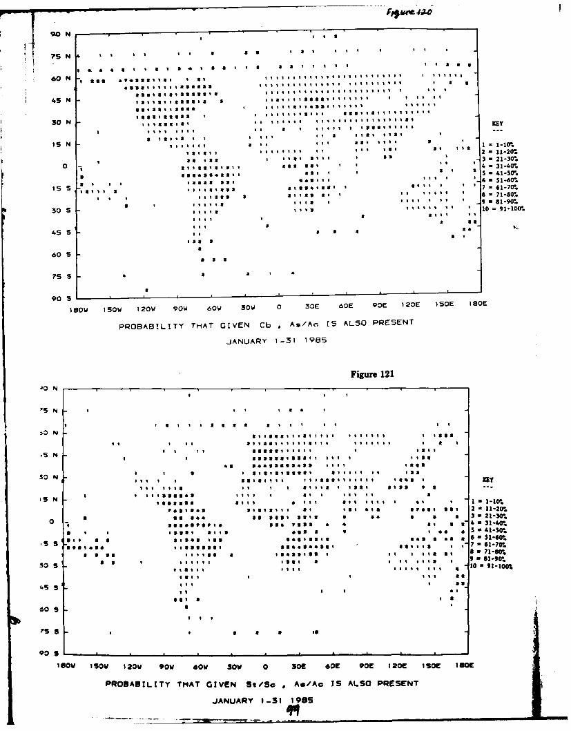
7S N •'

4S7 N a 1ai I a I gos I I I I I

I I t~ a42

30 N I I I t o I I I .I I I I I I . YI

1: : a I I I is I Im I , : I : I -

11m1111115 m 5! t iiimi mII i•i I S It m11 1

45Ntaimai5355 5m~iii3aliii Ii I t i t

30 N a ilt s I a I I I .I t t 1 l ii ml 8a il I 1 II l1 i l

S sI 1m i 111 ii 11m s2 -15015 N I i I , 1= It I *l

Is 5 t m s I3 5 21-30.0-0

a stsimsm ' 31 .0Is ItI lI I I 61_M

a as ss aI a' i 2 • s 41gas.

1 a1 5 I S I aI IIt - 6 1-9(.-1 1 I1133 I 5 11am1 S I I hS l I 71-7V

30 I I I5I I t S I I I I 10 I I 1 91-0.50 Sm i t , aiI iit i it 1 1-0"

45 S - a a a

II

60 S

?5S aIaIaII

90 5 i

l80W 15oW 120W 90w 60W 30W 0 30E 60E 90E 120E i50E iSCE

PROBABILITY THAT GIVEN Cb , As/Ac IS ALSO PRESENT

JANUARY 1-31 1985

Figure 121J0 N

Sa a

'5 N I t I 5 A

tt 5 t I tI 5 m a a , m m t a

:iO N altgatl l ~l mt 11 h u IIt m masis

Ia I it a li ItIt I I I I I 11111 1I i a

I N oI m i S m I si l l I o s s sa s * I a s1 Ii a 11 -0I

iiiImugii tIl 5 t1 i 1551tlll9

I timmaa mi It S ml IS mt mt a l

0 NII 5 5 a II I C m t I a m I I I I a i I 1-SPeatmamtsmal•lim t I ma im sp11 s, sat2"-"0t

0s ma3sa iai a a a a a 31-60.a I l l s m 11 g I I a a I 7

1 -0.meet 3. amaa m m a a ma a am m a a i i m S -|

aa i m a a s ommm a itl mi V ma 27.1-800.

SmIi mmtmi Il 1 5I I 4 Ii iS •I *-0?

• s u1 mittI41 Il a 10 9 1.1005 • 11111 iil • I i i sm 8"0)

S it I 35 0

4s m Lma as

al I mm609S

?S S • o90 S " I I I I I IIIII

905s

'60w ISOW 120W 90vw 60W 30W 0 301! 606 90 1206 10 SO 10

PROBABILITY THAT GIVEN St/Sc e Ag/Ac IS ALSO PRESENT

JANUARY 1-31 198S

Figure 12290 N

70 m a a a a a

12555a41 251I 55l 5 I l a 9 01 l II 7 2fllt l11-20%l*22*5QQIIlll5l I Stis Iitlll i ill alela I I 'll asall sas

60~~I as 4,a2a a3 3liaaa, 21s,2230125a.I 22l5t051S a tll t 41sI-50%232255 l 5 lli@ i ii' I • ,* * I 55.555

II II• , t t a sll a."s-4

al I 2 5 2 1 a, I t a 9 - 81-90%

Co s 5 =.. . ' 5• -l zlW30 IC~ s t 1I I a I5 a 101-00

I Illl I t I 2 2e at s • -05It 11%Ii111IISl I I 6*0

4StI I II II

4

l8ow I sot 120W 90W 60W 30JW 0 30E o .E 9CIE I120E i SOE I18("e

PR OBABILITY THAT GIVEN As/At C, /Cs/Cc IS ALSC P RESENT

JULY 1 -31 " 83

Fiur 11123'I

'S N

a 2 II1

! 5 S I I S

.3 NT N ,

I I I I I I I I

's N

•I I t I II

I 1 I I I 2 I1 I I I 1I lt! II I

t NI I I I IS SI II 1 I ll

0, 3, 21-301501 I

SN 11 1 151 11111 I I Ill I ll1

I a IUII I 1 I S I 2 I 1II 1 I s 1 I,,1 *I= -10%2 4 Ias I I I5 ,, P I, I Ct I I I I I 50 2 = 11-201%

O I I Is t1s I I 3 I 21-30%I 1 I , I I I I I & I 31-&0%

I It I I I III *4l-S%0%,5 S ' 6 3 1"6W.

'55 I I I I 1607

I I I I I I 7 61-70.

a i, I0 7 1-80%51 s 9-61-9%

O ,10 91-10w

4-S $ sS

60 S III

7'S S

I DOv I SOl 120W Plw 60W 30W 0 30E 601 90E 1 20E I 5OE I 80E

rIROBABTLITTY THAT CIVEN No , C,/Co/Cc IS ALSO PRESENT

.... . .. / .2 . ...-"

7 514 a , a * , a a 4 a , a .

em a m, a t a! sam a a a a a am a a 2

6 to weII 0.66 * 1I I I I I I an IlatI6 1 1 II8029992 N

:I : :i :I I:• : I : : 9 KEYQI I II l

14" •1 1 1 1 1 1 1 1 1 1 1 • l ~ l l l

of 1. 1 I I . 1 t1 1 l I: • ll l l : :.

0a ameeo a24 X a#maaamaaamma aa140aaaamm2m11a2Wt

0aa~aaa 989 a,96 poaam aoam a odemma aaa4m31-40

Is 4a-a7m a ' m a 'Olt ' It 1 1 o'- 7 6-70'

Is I 4 Iql Ia I I 1 9 S 1 1a 1*1 1 tl i •2 40 7-

30 S

meemmei, gatTII maaaamilma • IE2.3

9 C C Co a , s I mm a ,O i, S ,,• • 9, 19"

1 oaaa v maaa . a. W11 OI 1-0

7S S 6 • •o90 S a

S a , a a a a

21 11 1 10 lilt~ li e eat iia e -1W

45 N allIma hi aaaaa m14 ,11 as*2 * 9080

30 0 1 w0 0 a ama 60a9ama0g10 180 9

aJa a I I a I My

I5 ma : a t0 a, .

1 3igue 2 a

a t as1 I I I mo es total 1 • • • I tl I I it 40 a t •

60 5

82 2 6 *61*41 011 1 1 1 agol la a a l 41l l I II

11 18 1 !S I gas I $vstII Il l1 8I II a41 4 31 21-W.

11 I I I I I I I Ill l at a1 S- 4 31-40 .Ill l

I I

*5 S toI ! 1 I at 1 6 31 I lIll-W.~llS l l I

4S S

9 S

$sw I50w 120W vw 60W 30W 0 309 60E 90C 120 5C I OE

PROBABILITY TAT GVEN C , C/Cs/Cc iS ALSO PRESENT

11N11111 am I ll, 11 •1 s1 ai . •a I i | .0

I I IIII I I aJii a1I 1 am m mc a Ilm Illm a1 ca m'

(, ~ ~ ~ ~~JL 1-3 1983~llqS I. I 0

60 N1

C 'a'. iI i t, l amamamaamaaooa aoa-SOmo

ll,*Ul Ih • ' I I ,lmmlamalmllmaabaImmm1-90%

le aa a, ,t i , ,ii , , i , • lOa" t1-100

Wil mtI ,t aIm m ,

-o I .., i mai , mima ,ma' , a. a . a S 2 - 0

I o 0 0 i60t t 0W I I I 0[ I 0S 21 a 50 a a 0 *1[~ 0

t I JU Y I-3 71-90

30 ~t * a a 10 *9110

S t Ii ii ii

0S N aa3 0 0 a

a a * • . 3• a a 3 0 a aa I 0 I a a a 1 2 0 a

I N 2 0 0 0 0 0 0 0 9 * 0 0 0 0 0 0 0 0 0 0 0 0 0 0 0 0 0 3

03:a30100010 00000 00001gas002

300000 7 0**as a 3 21-311023

5 4 N • • • • 000000• 4 • 0 0 ! 30 30 ! 8 • 2s •

943333Is 00033 IS30 45 3300 1-4(r9a0 a o a1 a. 3 4a a 31 033I4 1S S 2 11-50.

is08 3 as50 30 6 5 O 1-0.7390a7007 61-7003 3

3 *

aI *1 IIIII 112 0$I0i 0 0 0033I 1 00 51-O

0 3 0 2I 9 81-90

5:0 0 00000 I I I 0000aI 10 *91-100%

.45 a a

?S S

1 80W ]sow 1 20W 90W 601a 30w 0 30E 60E 90E I 2CIE 150E I 80E

PROBABILITY TriAT GIV~EN Sr/Se C&/Cs/Co 1S ALSO~ PRESENT

JULY 1 -3 i 1983

Figure 12790 N

00 , 0 a , a 2 i 02. 0

60 N

100000-8 033333o033333......33 3139333 33... .. 0 1 '

is N t I I I I a sea&$ s 9= 2-0

lossa *$ 9 6 1 9 a , , 0323

1 I ag i.a t e 2 11:2C

0S No * 3 21 33c0

0 0 0 0 0 0 2 0

43 21-40

les -S S s S : a309 a 0 3 2 3 S 4u1-S0

is P 633320 31-6C1 9 3 o

SOSO- 0 : 033 : g 80093 a3 7 6~.1:70

0 0 0 00 a033•a0I I a300383190.

'Is000F •

a3n 10 0 0 3

405 S

0 S

?S S

905S

1I0W ISOt 120W 90w 60W 30W 0 0O 60E 90! 1206 150E 1I0E

PROBABILITY THAT GIVEN Cu , A/Ac IS ALSO PRESENT

JULY 1-31 1983

90 N , ,a...a

a

60 N bt a a a a a I I a a I a a a

m a a aa• i•a a a a i I t t a I a t ma a a60 N

aa IaIII m Itl I I It 12 t 1 1S I tala

t Ii t , I 2 1 1 1a1 t%5 N I I I I I I I IItam1 I I

15 Na timllli a,.,,,, a i aa mlll

3 0 N l l l

0I- I I taa, u mm a a a aill ' i

)S N I I I I! i 4 S t KEY

a I I t I I * I t I I I t I I a t tl aI 10I sI I I I ,l ail l tl•a , a I 4 = 314

i llaia a II It8 II i I II 6 I 1-60

0 I2 a=11-20%• , Ii I , ii • 3 =21-3M%1 ,, tml . i • . i 4 31-40%I s S "S In 4 1 i Iis $ & - 0 %

u a I I , a a • i , , , t i t i i 6 5 1-W.

* a i • t I I I a ' t 7 = 61-7(O30 S 0 2 2i1 Ii I 18

• i ,, ,• i , ! 9 6 1-90%

45S a ; a 12 = 91-100%.att a a am

60S a

?S5 . , . t I .

90 5

180W 150W 120W 90W 60W 30W 0 30E 60E 90E 120E 150E l8o

PROBABILITY THAT GIVEN Cb , As/Ac 15 ALSO PRESENT

JULY 1-31 1983

Figure 12990 N

7S N a I6 Na

75 N I I I I I a a s I I I I I tSi a a l a a am a I a all7 :19 1 a a I a I a Im a t

60 N Is am4~ : aaa s a m a m a a m a a t -t 2 11:2

45 N I Iti lt t lI taI ItI t om i I I 3I0'30 N a I I I t I I I I I a la, t t • a60

ttl1 mama t ,, 1ia mamammamltala a a KEY

aal '2 m 1 aaa ama1 a8

4S N I

amamaS aaa•aalinat ami t *lm ama•1• -I

0 11-20aammattm aa•* a ie It a a. •31-40

a5$ I t ' amma, , a thini I ma 6 S, 1.30

~*I ~t l~at~~t tiltl I 71-70I I I 'im, t ~t ~ ~ 6 71-8030 S a ' m, itt a t t a t 19

t I, a,,11 U 0m9-

45 5I i amam, I I a

b 60 5

I I I

75 S

90 5

10w s50w 120W 90W 60V 30W 0 30E 60E 90E 1 20E 150 E I80E

PROBABILITY THAT GIVEN St/Sc * Au/Ac IS ALSO PRESENT 1,.-JULY 1-31 '3 *093

Figure 130* -,.- - - - - ,.---------------

7S N 2 1 2 "

45l N

1 .2 90 301 3 96

15 N 336'~ S90 13 / 2 $, low

0 42 47 0 ,5 1-

2I 1, 1 1v; 1-53.. 4. 2 1 23 / 2t

1.31

.53t5

45 5 --

1 93W 15w ?')W 90W 6-)W 30~W D.3~ E -;:E 12Oct 15,E 1 80E

irISTIBUr'(N OFr SYNOrTT~C r-SEVAT!ONS !N TENS

JU&"y 1-i1' Figure 131

75 N 2 ~ .*

45 N -3 2 227 1 1 1 40 2

2 233*270 29h 7' 7 1 9111A 325 2 2 I.N t- 2 3

t6 1

15 K2 A2 22 s

2 3

[. 160 s

160w 150w I?,W Prw 60W 19ow 0 30C '30E 90E 120E ISOE 10!

CI!ST19UTIrN rF SYNOPTIC fR'SERVATI1'NS IN TENS

JANUARY 1-31 19P5

L-11 I of

7S N

160 N

45 N Iw el

30N

T SN

IS NSs

30 S c

60 S

4S S - i

905s

180W 15sow 120W 90w 60W 30W 0 30E 60E 90E 120E I 50E I 80E

FREQUENCY OF OCCURRENCE (PERCENT) OF C. /Cg 'Ca ONLY

JANUARY 1-31 1Q85

Figure 132

90 N

60 N

45 N

20 Io3s30 N

IS N so2

0-

30 S

60 S

4S S -7

90 s

110W 150Wd 120W 90W 60W 30W 0 30E 60E 90E 1209 150! 160E

FREQUENCY OF OCCURRENCE (PERCENT) OF Ag/Ac ONLY

Figur 133JANUARY 1-31 1985Figur 133105

* .---..-..° ".------- .--

60 N

45 N -

s0 N 3

0 17

Is -,

45 S

60 S

90 5

180W 1SOW 120W 90W 60W 30W 0 30E 60E 90E 120C 150E 180E

FREQUENCY OF OCCURRENCE (PEQCENT OF NIMBOSTRATUS ONLY

JANUARY 1-31 1985

Figure 134

30 N

75 N 33

60 N

2 3 l a 10 k

4S N l 57 • l s

&31 40 33 .s ,o0 42isos s

60 S

as0W so 120W 90W 60W 30 0 30! 80! 90! I0! 150! 10!

FREQUENCY OF' OCCURRENCE (CPERCENT OF CUMULUS ONLY

-e 135 2 JANUARY t-3 985

30 s -

n ro o ST 100 s Sao S&0s4S58 o 11

~6 S - to • 3 .. . ? "-, - -.. . .to----o--- - - - - - -- -. - . . . -

Figure 13690 N

75 N I

60 N -1-r 2

30 N ao &32

IS N109t a

25 -w 50 672

so S -i T c b

60 S 3 1. to

.V5 S

90 S

I8ow 150W 120W 90W 60W 30W 0 30E 60E 90E 120E 150E 180E

FREQUENCY OF OCCURRENCE (PERCENT' OF CUMULONIMBUS ONLY

JANUARY 1-31 1985

Figure 137

75 N

60 N -] S o

*03530 N 49 20 112 63

is N .S 25 is1 3

0-.

7557

30 S160W~t so0 at0 90o itW t0o 0 0 0! 10 5! I

4SQUNC OS OCUREC (RCNTO 1:S ONL

JANAR 1-S 19

so1

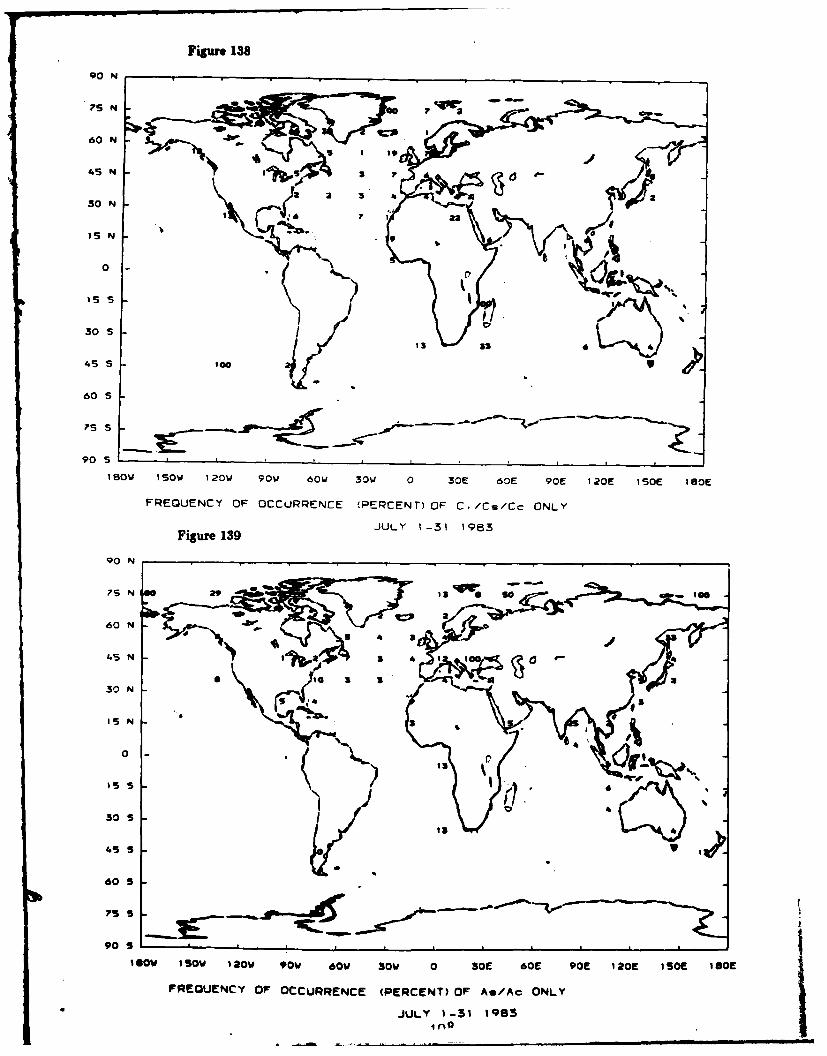
Figure 138

90 N

1~~5 N %"°

60 N

4S5 N 3.0

so N

15 N

0-

3o 4

45 S 10

90 s

1 sow 150W 120W 90W 60W 30W 0 30E 60E 90E 120E I SOE I OE

FREQUENCY OF OCCURRENCE (PERCENT) OF C./Cs/Cc ONLY

Figure 139 JULY 1-3| 1983

90 N

7S N 00 13a-o1 0

60 N 4S N

4S N IA

o . i -30 N

Is N

0-

Is s

30 s

60 S

90 S

lOW $sow 120W 90 0W 30W 0 30E 60! 90E 120E 150! 180E

FREQUENCY OF OCCURRENCE (PERCENT) OF As/Ac ONLY

JULY 1-31 1983Ina

90 N

75 N

45 N

30 "

tmJ N13 9IN.N

0-

Is s

30 S

45 s 31

60 S

90 .

I80w 150W 123W 90w 60w 30W 0 30E 60E 90E 120E ISOE 180E

FREQUENCY OF OCCURRENCE fPERCENT) OF NIMBOSTRATU-5 ONLY

Figure 140 JULY 1-31 1983

60 N -

60N0

0 a '

n~ ~ ~ ~ ~ fi f07so 7

05L0 f

'160W 150 1~ 20W 90W 60tW 30W 0 ! OC 601 90E: 1 OE: Igo tOe: OEFREQUENCY OF' OCCURENCE (PECENT) OF CUMULUS ONLY

IsJULY t-S 183

; 10r 14110 94I

4S S0.

|g N

?S N

60 N

.4S N - -0Io

5) 5

30 N 0

30a "sa

905

180W 150oW 120W 90W 60W 30W 0 30E 60E 90E 120E 150E 180O!

FREQOUENCY OF OCCURREmNCE (PERcENT) OFm CLJM'L0NTMBUS ONLY

Figure142 JU1Y 1-31 1983

90 N

30 . . ..00

75 N I'

o 124S S - 1 Itoq

60 N

6

7S S

90 S

Isl @OW 50 120W 90W 60W 30W 0 30E 60E 90E1 !20E[ IS01 160E[

FREQOUENCY OF OCCURRENCE (PERCE'NT)01 CUMUL S=ONIMUYOL

Fiue12JULY 1-31 1983

90 N0

6 0 N t o? ~ 1 6 .0

4S ~ 1 M ' 1

30 N - 29s a 64

IS N - 1 5 1 t

0-0

i5 S I ar

80 S

4S S -10 3 o

90 S -~ ~:I-

Is0w 150W 120W 90W 60w 30w 0 30E 60! 90! 120! ISOE ISGO!

FREQUENCY OF OCCURRENCE (PERCENT)OF St/Sc ONLY

JULY 1-31 1963

Figure 143 1

,, - -, ,gureiw - - - -

90 Nso

7S N O q*t e*

60 N4aa a1

4S5 N . 20 12 '7i

SO~ ~ Fgr Me145 4 0 10 N

SON -. I •

IV 67t 12 2j, 21 i

is N - is 25 4s 1

i s is

4S S -

60 S

90 S ,i,-ii,

I sow I sow 120W 90W 60W 33W 0 30E 63E 90E 120 I S10 I SOC

PROBABILITY (PERCENT) THAT GIVEN A/Ac , C/C/Cc IS ALSO PRESENT

JANUARY 1-31 1985

Figure 14590N

7S N

60 M

4S N a 11111

30 N "-

leea

is:S

30 S

60 S

SeOW 150w 120W vow 60W sow 0 sot 606 906 1206 50E low

PRODABILITY (PERCENT) THAT GIVEN No *CI/Ce/Cc IS ALSO PRESENTJANUARY 1-31 196S

lit

QON Figure 146

75 N

60 N

310 N ~-~ss

- 0 tO 10050 60 .,m

30 7N766 6

*#a~~~~s 6046P& 3 1 2 os

too t0o so6 3 6

It0 o 73 s 6 23 67 1

so oo

45 5 sos 2 ; 73

60 S

180w 150w 120W 90W 60W 30W 0 30E 60E 90E 120E ISME 180E

PROBABILITY PERCENTY TH-AT GIVEN C.j ,C./Cs/Cc IS ALSO PRESENTJANUARY 1-31 1985

Figure 147

00 N

60 N

45N1 a 20 Iw 0t 01

30 N-

1 5 NS a

30 S

so.J

4S S

60 9

Isow IsOW 120W 90W 60 3oy 0 30! 80! 90! 120! I50! Ig0!

PROBABILITY (PERCENT) THAT GIVEN Cb *Ci/Cs/Cc IS ALSO PRESENT

JANUARY 1 -31 198S

Figure 14890 N

Web.

60 N

al is I ,I s a' s* I//

30ON ; ' Z 4IS N 010 100 20 1. 2l

33 2S 23 J i

so

4S5 S 6

605S qL-.

75 S

90 5

180w Isow 120W 90W 60W 33W 0 30E 60E 90E 120E i SOE 180E

PROBABILITY PERCENT) TiAT GIVEN Sc/Sc , C,/Cs/Cc IS ALSO PRESENT

JANLJAY 1 -31 1 985

Figure 149

90 N

7S N

60 N

30 N

30 N

iiUsV t- I le S

30 1

-s 101

IS S I p

305S

ISoo Is0w 120w 90V 60W 30W 0 30C 60E 90C 120t I90 100loo

PROBABI1LITY (PERCENT) THAT GIVEN Cb *As/Ac IS ALSO PRESENT

fANUARYf -31 198S5

Figure 150

90ON

60 N

30 N

40 N0 20£02

30 J

0 4

1ANA0 i-3 19085 3

60 N

30 N

155Figure 15190 N 0

60 N

455N8 4sa

is0 10 120 toW 60w 30 0 0 0E 10 S!

P3BA0LT (PRNT -HA JIE tS sA SAS RSN12~~JAUR 30E Is4 9852as 7 it I

Figure 152

90 N

60 N

30 N

Is S 7132 2 S

30 c

30 S

90 S

?S S

60 S

160W 150W 120W 90W 60W 3OW 0 30E 60 90 120E 150 10E

PROBABILITY (PERCENT) THAT GIVEN CuA , CiC./Co/C IS ALSO PRESENTJULY 1-31 1983

Figure115

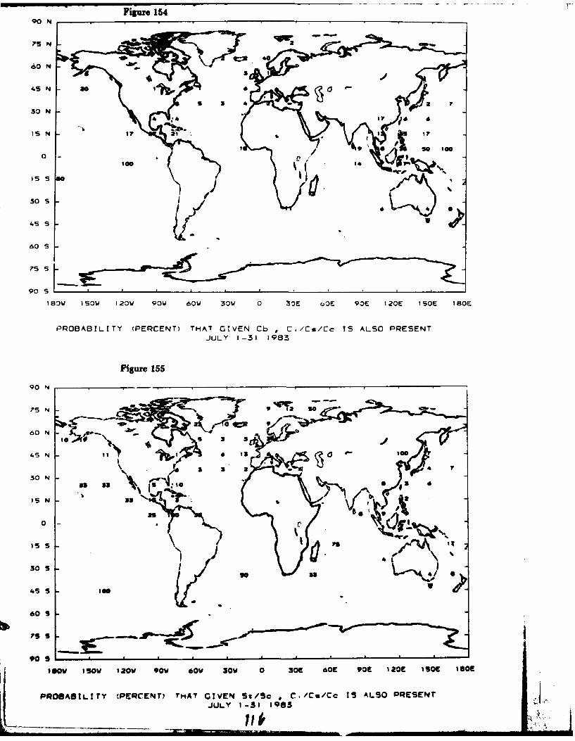
Figure 15490 N

?S N2

.60 N

30 N

IS N

30 S

605

75 N uI

60 N -

45 N

75 N 9% 2 so%9l

60 N k40

IS S

60 S

IsS To

90 S

,.ov I50W 120W 90W 60W 3OW 0 30! 60! 90! 120C MEO 16

PRosAS IL IT Y 'PERCENT, ?tiAY GIVEN Sc/Sc *C./Co/Cc IS ALSO PRESENT4JULY 1-31 1983

il

Figure 158

90 N

-30 N

0033(76 so3 s

40 S7IsS

40 ~~so20003 2Ss30 S - 0010 29 9 3

45 S -

60 S

90S

180W Is0w 120W 90W 60W 30W 0 30E 60E 90E 120E 1SOE 180E

PROBABILITY CPERCENT' THAT GIVEN Cu~ As/Ac IS ALSO PRESENTJULY 1-31 1983

Figure 15790N

20 N7

30 N

4S NS 0 I 61

305 N'1'a s

rOs:: : ,,~ 0! 0! 9! ~~50!I1O

60 N

30 N

60 N

iS N s

as 030 N

45 5 s 5 I

60 S 402

75 S

l80W )sow 120W 90W 6OW 30w 0 30E 60E 90E 120E ISOE 180E

PROBABILITY (PERCENT) THAT GIVEN St/Sc ,Ag/Ac IS ALSO PRESENTJULY 1-31 19B3

Figure 158

Q0 N

7S N OF 72 3 03

60 N

4S N 79&7 100 ~ (~6S 9 1 r7

30 N a 972 00 ve 92 OS *7 49 *47 *9 TO :1 ,. ., S G 7 s. s ,. so So3, so so

ISN I at 40 "so do 40% so3 *a 4 63 so , . a.

25 s so 4 .7 \7svti 4,1 i 7 r s

a5 s 3 so *7 710 s0 *0 or 7 , ,

5 3s 0 rs 43 , 61007 " 9 O 3 5 s9

60 SIce ,IS Smice 94 ce is &0

75 S

905S

180W 150w 120W 90W 60W 30W 0 30E 60E 90E 120E 150E 180E

MEAN TOTAL CLOUO AMOUNT (PERCENT) JANUARY 1-31 1985

Figure 16090 N

60 N TSR Is Cap

30 N

0-

1 1551 39 70 59 74 .1 al 63

SD4 go 394 031S2 54 1 S 4

60 S

is0V 150W 20W 90" 6sW Slo 0 3so 60 90S m0ug ISOl I

MEAN LOW CL=OU AMOUNT (PERCENT) JANUARY $-11 19s

~119

I __ __ . , , . , . , __ ,,, , %,, , * - ~ -/

Figure 161

.SO li 1.4 A '

6C ~ ~.4\~,',, -

454 ' 5 .. - ,

6C N a-- ME Q- \rst= so .00

4S N 0e 00

0 S N so

r0 so' ~0 as i~'6

I5S N to

S4w AA

SO- s

1000

, • _ _._ F-------------- L- --------- -- ' " - ' - -- -

MEArl MICOLE CLOUID AICUNT IPERCENT JANUARY 1-31 1985

Figure 162

75 N

60 N b

3C N .110

11;7

-'so

51 N 0

0- K Z. ..ib

605

75s S*~ as.r~~S 4*' -~-

90 S

Is0W 150ow 120w vow 60W sow 0 30! 60E 90! 120! 150! tISO!

MEAN HIGH CLCUD AMCUNT (PERCENT) JANUARY 1-31 1985S

Figure 163

90 N

60 N

4 ~5 N G5O 3 Go re 3443 7

- .3643 -, ISO *I, " Se705 s07

905Stiv i "

180W 15SOw 12C'.W 90w 60w 30w 0 30E 60E 90E 12CE 1SOlE 1BOE

MEAN TOTA, CLOUD AMOUNT CPEIPCENT) JULY I -31 1983

Figure 1640 N

M~~~ iti*S 0i 1S

75 N so I

60 N

I0 v g I IP s 1

0 a rs 41 * Sf-n 3 9 1 7 o o

30 N 52 --o s s ft so Sl . s *I 4 S 4

5 7S 16 00S a a s If45 S. too 03 * Sol

60, a 13 4 99 6353 45 3

0 5 6 334

180w I sow 120W 90 60 30W 0 30! 60! 90! I 2 0 I SOi I OE

MEAN OW~t CLOUD AMOUNT (PERCENT) JULY 1-31 193 I

Fiur 1

90 ' N':

7S N

"~ ~ ~ ~ ~~s Ipii To- i i -I i I i

Figure 165

60 N ,

4S N~ so*'I

.N k4 """." -

C , - C) asSI A t ; -"%7o w

,SN a" a s a..,

45 S -

1 901. 15010 120W 90W 60 1 30W 0 31,E 60E 90E 120E I Sot 180E

MEAN MIDDLE CLOUD AMOUNT tPERCENT) JULY 1-31 198

7S N

-- , ( .a,\," - 2'€., .. i ' '€,

Zoo " ,

60 Sb s l.1

45 - ----

ia s- o 188

is N

60 N

0 S 1s o t 6 E .E 1 2SC , N a. "

,, -- I , IL 2 II I I

3 ow )SOW I 2CIW vow 60V low 0ME0N HIGH 9 AJ 1

MEAN MICIM CLOUD AMOUN.T (PERCENT) JULY 1-31 1i 3

The climaologiss buat-up fromn only aL couple Of months of data are of insuffiient timepan

to be of longstanding use in climate modelling exercisess but can provide scope for tsopria

with satellite data in exercise such s the evaluation of new retrieval algorithms.

4. Suummary ad Cosclugloms

b A prelimnarsy isvestigatioa bst cetain far-- of bias bows to a~sct surface observations at

xlusbs4 made oung two separate matshs of global cloud reports. A search for evidence of

nighttime detsction him gave variable resulfe but ov the ainalysis regionat Scandiavia where the

evidence would be stirongest, due to the ability to compare reports over short amd ln nights, there

wa good reaon to believe t"a observers were coassenty failing to detect cirrus (partiularly)

and altostrasus at the local scable wolf as over larger area. If such bias ns prevalent over may

egosof the world the value of surface-derved climatolosiee mvust be reduced.

Contrary to earlier assertions, contingency probabilities (and the associated rik of partial

NcAs bias) were generally found to decrease for higher amounts of lower cloud, a reult and

sugesin that further examination of cloud data sets is required. The role of contingency probe.

bilitiss should be established further, especially with regard to obscuring overcasts.

2 Finally, the global data were assembled into maps depicting frequency of occurrence, contin-

gency probabilitis and level amounts. The data highlighted such features as monthly variability

compared to long-term statistics and the paucity of oceanic data, which awe overall, unreliable as

a result. The land data are more repesnttie and may be of use when resuits from EIR are

released.re VIP' Ot1

123

a. frementationas and Publications

Constructing global nephanalyses: a review of recent progress in cloud detection and

analyids, A.H. Goodman and A. Henderson-Sellers, Thirteenth Annual Conference of

the Remote Sensing Society, University of Nottingham, 7-11 September 1967 (poster,

Global cloud data: problemas In synthesis of heterogeneous sources, K. McGufie, A.H.

Goodman and A. Henderson-Sellers, Twenty-First International Symposium on Re-

mote Sensing of Environment, Ann Arbor, Michigan, 26-30 October 1987 (poster and

oral presentation)

An investigation of bias In surface-observed cloudiness for the globe for July 1963 and

January 1965, Ali. Goodman and K. McGuffie, Clouds in Climate 11 Workshop,

Columbia, Maryland, 19-23 October 1967 (oral presentation)

The problem and bemdits of combinng heterogeneous data sources Into global neph-

analyses, Ali. Goodman, seminar at AFGL, 26 October 1987

PSh&C~Sip

Cometructing global mephanalysest a review of recent progress In cloud detection and

analysis, Ali. Goodman and A. HendermoD-Seflers, 1967, In Aivesoee is Di#"ta

hnae. Pmern#, Remote Seasing Society, London, 446-452

Global cloud data: problem In synthesis of heterogeneous sources, K. MeGuffie, Al.

Goodman.said A. Hendersners, In Pmending. of Tweatr-Firt International

-ph-sms on Reaskt Sesing of Ismresuest, Ass Arbor, Michaige

Clouds hr dlinmto recet progres In cloud detection ad analysis Ali. Goodman and

A. 22-2ruo- 8 6 su vbmitted to Atmspheric Reearh

124

6. Kehfenmf

Arking, A. and Childs, J.D., 1965, Retrieval of cloud cover parameters from multispectral satellite

measmnts , J. Clim. Alpl Met eor., 24, 322-333.

Berlyand, T.G. and Strokina, L.A., 1980, Global distribution of total cloud amount, Gidrometeois-

dat, Leningrad, 72pp.

Brooks, C.E.P., 1927, The mean cloudiness over the earth, Mem. Roy. Meteor. Soc., 1, 127-138.

Bunker, A.F., 1976, Computations of surface energy flux and annual air-sea, interaction cycles of

the North Atlantic Ocean, Mon. Weather Rev., 104, 1122-1140.

Chahine, M.T., 1962, Remote sounding of cloud parameters, J. Atm. Sci., 29, 159-170.

Chou, M.D., Childs, J.D. and Dorian, P., 1986, Cloud cover estimation using bispectral satellite

measurements, J. 0kim. AppI. Meteor., 25, 1280--1292.

Coakley, J.A., 1987, A dynamic threshold method for obtaining cloud cover from satellite imagery

data, J. Geephpe. Res., 92, 3985-3990.

Coakley, J.A. and Bretherton, V.P., 1982, Cloud cover from high resolution scanner data: detecting

and allowing for partially filled fields of view, J. Geephya. Res., 87, 4917-4932.

Cox, S., McDougall, D., Randal, D. and Schiffer, R., 1987, FIRE - The first ISCCP regional

experiment, Bull. Amer. Meteor. Soc., 68, 114-118.

Dusbois, M., Sim., G. and Szejwach, G., 1982, Automatic classification of clouds on METEOSAT

imgr: Application to high level clouds, J. AndI. Meteor., 21, 401-412.

Vye, V.K., 1978, The AJ'GWC auto~mated cloud algsis modek A.FGWC TM 76-M0, AFGWC,

Nebraska, 97pp.

Godshall, V.A., 1971, The analysis of cloud amount from satellite data, 2lei. Now York Aced.

Sci., 33, 436-453.

125

Hahn, Cj., Warren, S.G., Lou, J., Chervin, R.M. and R. Jene, 1962, Ad" of swssulameou.

occurrence of different dlea trpe our tic os, NCAR:TN-201+STR, NCAR Tsch-

nical Note, National Center for Atmospheric Research, Boulder, Colorado, 34pp and

Is$ map.

Hahn, C.J., Warren, S.G., London, J., Chervin, R.M. and R. Jenne, 1964, AU...!o .smuftseou.

occurrence of different cload tipes oer land, NCAR: TN-241-STR, NCAR Technical

Note, National Center for Atmospheric Research, Boulder, Colorado, 21pp and 188

am"p.

Hastenrath, S. and Lamb, P.J., 1977, Climatic Atlas.f tic 2~opical Atlantic and Eastern Pacific

Oceans, The University of Wisconsin Press, l5pp and 97 charts.

Hendersonk-Sellers, A., Sloe, G., Drake, F. and Deebois, M., 1967, Surface-observed and satellite-

derived cloudiness compared for the ISCCP special study area in Europe, J. Geophgya.

Res., 32, 4019-4=3.

Hendersou-Sellers, A. and Hughes, N.A., 1965, Global 3ID-nephanalysis of total cloud amount

climatology for 1979, J. Clin. App$. Meteor., 4, 669-686.

Hoyt, D-V., 1977, Percent of possible sunshine and the total cloud cover, Mon. Weather Rev., 105,

648452.

Hughes, N.A., 1964, Global cloud dlimatologiss: A historical review, J. Chss. Appl. Meteor., 23,

724-751.

Inae, T., 195,0On the temperature and emissaivity dtriaonof smil-transparent cirru clouds

by bispectral mesrement i the 10 micrometer window region, J. Met. Sec. Japs,

a1, W-102.

Liona, E., 1964, Proesseed setelite inmaerie for operational jorsesdti, SMHll, Swedish Mesteoro.

logical and Hydrological Institute, Norkoping, O3pp.

i z

las, E., 1986, Use of the AVHRR $.I micrometer channel in multpectrL cloud classifetion,

SMHI, Swedish Aetorlogical and Hydrological Institute, Norrkoping, 23pp.

London, J., 1957, A study of he atmoaperie keat alie.e, Final Report, contract AF19(122)-165,

College of Engineering, New York University.

Malberg, H., 1973, Comparison of mean cloud cover obtained by satellite photographs and ground-

based observations over Europe and the Atlantic, Mon. Weather Rev., 101, 893-897.

Malick, J.D., Alle, J.H. and Zakanycs, S., 1979, Calibrated and analytical modelling of cloud free

intervals, Proe. Soec. Photo-Optical Instrumentation Engineering, 195, 142-147.

Quayle, R.G., 190, Climatic comparison of estimated and measured winds from ships, J. AppI.

Meteor., 19, 142-156.

Reynolds, D.W. and Vonder Haar, T.H., 1977, A biapectral method for cloud parameter determi-

nation, Mon. Weather Rev., 105, 446-457.

Riehl, H., 1947, Diurnal variation of cloudiness over the sub-tropical Atlantic ocean, Bull. Amer.

Meteor. Soc., 2, 37-40.

Romw, W.B., Wloshar, F., Kinsella, E., Arking, A., Desbois, M., Harrison, E., Minnie, P., Ruprecht,

E., Sine, G., Simmer, C. and Smith, E., 195, ISCCP cloud algorithm intercomparison,

J. LIm. AppL Meteor., 24, 877-003.

Saunders, R.W., 1906, An automated scheme for the removal of cloud contmination from AVHRR

radiances over Wester Europe, lot. J. Remote Se"*#s, 7, 867-86.

Sauders, LW. and Kribd, K.T., 1967, An improved method for detecting clear sky and cloudy

radianeshao AVHRR data, jL J. Rtmode Sesfem (in press).

Shr, R.A. md bRea, W.B., 10, The hntational Satellite Cloud climatology Project, the

5mM project at the Worl Climate Research Program, Dl.Amter. Metewr See.# 64,

f79-784.

127

Starr, D.O., 1987, A cirrus cloud experiment: Intensive field observations planned for FIRE, Bull.

Amer. Meteor. Sec., 68, 119-124.

Warren1 S.G., Hahn, C.J., London, J., Chervin, R.M. and R. Jenne, 196, Global dutribution of

total cloud cover and cloud type amounts over land, NCAR:TN-273+STR, NCAR

Tlechnical Note, National Center for Atmospheric Research, Boulder, Colorado, 29pp

and 199 maps.

Warren, S.G., Hahn, C.J., London, J., Chervin, R.M. and R. Jenne, 1987, Global distribution of

total cloud cover and cloud type amounts over the ocean, NCAR Technical Note in

preparation.

World Meteorological Organization, 1956, International Cloud Ad"a, Abridged Atta, WMO,

Geneva, 62pp and 72 plates.

World Meteorological Organization, 1974, Manual on code., Volume 1, (WMO Publ. No.306),

WMO, Geneva.

World Meteorological Organization, 1984, Manual on codes, Volume 2, WMO, Geneva.

World Meteorological Organization, 1987, International Cloud Adla., Volume 2, WMO, Geneva,

212pp and 196 plates.

1 -8

! I'