nonstationarity of real exchange rates in the g7 countries: are they cointegrated with real...
TRANSCRIPT
JOURNAL OF THE JAPANESE AND INTERNATIONAL ECONOMIES 11, 523–547 (1997)ARTICLE NO. JJ970396
Nonstationarity of Real Exchange Rates in the G7Countries: Are They Cointegrated with Real Variables?*
Masahiro Kawai
Institute of Social Science, University of Tokyo, 7-3-1 Hongo, Bunkyo-ku,Tokyo 113, Japan
and
Hidetaka Ohara
Faculty of Business and Commerce, Meiji University, 1-1 Kanda Surugadai, Chiyoda-ku,Tokyo 101, Japan
Received January 6, 1997
Kawai, Masahiro, and Ohara, Hidetaka—Nonstationarity of Real Exchange Ratesin the G7 Countries: Are They Cointegrated with Real Variables?
Using monthly data for the G7 countries in the post-Bretton Woods floating rateperiod, this paper demonstrates that almost all bilateral real exchange rates haveunit roots and, hence, are nonstationary. Consequently, it rejects simple PPP as along-run relationship. The paper also shows that many of these real exchangerates are cointegrated with other real economic variables such as relative laborproductivity, terms-of-trade ratios, real trade balance ratios, and long-term realinterest rate differentials. In particular, relative labor productivity is statisticallysignificant with the correct sign for more than half of the country pairs for whichcointegration is confirmed. This finding lends support to the Balassa–Samuelsonproductivity-bias hypothesis. These results imply that nonstationarity of realexchange rates and the consequent rejection of simple PPP can be consistent withthe notion that real exchange rates revert to an equilibrium in the long run withoutdeviating arbitrarily far from this equilibrium position. J. Japan. Int. Econ.,December 1997, pp. 523–547. Institute of Social Science, University of Tokyo, 7-3-1Hongo, Bunkyo-ku, Tokyo 113, Japan, and Faculty of Business and Commerce,Meiji University, 1-1 Kanda, Surugadai, Chiyada-ku, Tokyo 101, Japan. 1997
Academic Press
Journal of Economic Literature Classification Numbers F31, F32.
* This is a revised version of the paper presented to the NBER–TCER–CEPR trilateralconference ‘‘Purchasing Power Parity Revisited: Exchange Rate and Price Movements, Theoryand Evidence,’’ which was held in Tokyo on December 20–21, 1996. The authors are gratefulto Colin McKenzie, Shinji Takagi, and other conference participants for their helpful commentsand to Andrew Robertson for editorial assistance.
5230889-1583/97 $25.00
Copyright 1997 by Academic PressAll rights of reproduction in any form reserved.
524 KAWAI AND OHARA
I. INTRODUCTION
This paper offers tests for cointegrating relationships between real ex-change rates and a set of real economic variables for the G7 countriesduring the post-Bretton Woods floating exchange rate period.
Recent studies on purchasing power parity (PPP) or real exchange ratebehavior have analyzed time-series data either by conducting cointegrationtests on linear combinations of the nominal exchange rates and nationalprice levels or by applying unit-root tests to real exchange rates. Someauthors have found cointegrating relationships between the nominal ex-change rates and national price levels but that these relationships do notsupport unitary coefficients on these variables (see Baillie and Selover(1987), Taylor (1988), McNown and Wallace (1990), and Crowder (1996)).1
Although long historical time-series data may indicate that real exchangerates do not contain any unit root (Froot and Rogoff (1995) and Lothianand Taylor (1996)), researchers have generally found that real exchangerates for many countries in the post-Bretton Woods era do contain a unitroot (Corbae and Ouliaris (1988) and Mark (1990)). Introduction of astructural break in cointegration tests or unit-root tests does not seem toalter this general conclusion (Boucher (1993)), though there are a fewexceptions (Ceglowski (1996)). These findings imply basically that realexchange rates are nonstationary, contradicting simple PPP as a long-run,stable relationship. Simple PPP requires that real exchange rates be station-ary and revert to long-run, stable trends with short-run fluctuations aroundthese trends.
Rejection of simple PPP, however, does not imply that exchange ratesdeviate from, and never revert to, any equilibrium relationship. On thecontrary, the nonstationarity of real exchange rates can be consistent withthe presence of long-run equilibrium relationships. The reason is that non-stationary real exchange rates can be driven systematically by nonstationaryreal economic variables. In such a framework, simple PPP should hold inthe long run if the dominant shock to an economy is of a monetary type.If the shock is real in nature, simple PPP does not obtain.2 For example,
1 However, Johnson (1990) and Kim (1990) conclude that PPP holds in general. Kim alsofinds that the nominal exchange rate is more strongly cointegrated with the WPI ratio thanwith the CPI ratio. See Froot and Rogoff (1995), Taylor (1995), and Rogoff (1996) for surveyson PPP and real exchange rate behavior.
2 Such a view is incorporated as a maintained hypothesis in the work of Clarida and Gali(1994). They assume that real shocks affect the real exchange rate both in the short run andin the long run while nominal shocks affect the real exchange rate only in the short run.Based on the real exchange rate and nominal variables such as the relative money supplyratio and the long-term nominal interest rate differential, our preliminary investigation ofcointegration reveals that the real exchange rate is not cointegrated with these nominalvariables. That is, nominal shocks do not affect the real exchange rate in the long run.
REAL EXCHANGE RATES IN THE G7 COUNTRIES 525
the productivity-bias hypothesis proposed by Balassa (1964) and Samuelson(1964) suggests that cross-country differences in productivity growth sys-tematically affect real exchange rates through interactions between thetradables and nontradables sectors in each economy (see Bahmani-Oskooeeand Rhee (1996) for the case of the Korean won). Movements in theterms of trade reflecting changes either in supply and demand in the worldcommodity markets or changes in the tradables sector’s productivity forboth domestic and foreign economies can affect real exchange rates. Re-flecting the underlying cross-country differential in the marginal productsof capital, the real interest rate differential also affects real exchange ratesby inducing international movements of capital. See Obstfeld and Rogoff(1996, Chaps. 4 and 9) for a concise explanation of the effects of changesin productivity, terms of trade, and real interest rate differentials on realexchange rates.
If nonstationary real exchange rates are cointegrated with a set of nonsta-tionary real economic variables, real exchange rates cannot be said todeviate from equilibrium relationships in the long run; real exchange rateswill revert to equilibrium without wandering too extensively for too long.The objective of this paper is to examine if real exchange rates are indeedcointegrated with a set of real economic variables, such as relative laborproductivity, terms of trade, real trade balances, and long-term real interestrate differentials, for the monthly data from the G7 countries (Canada,France, Germany, Italy, Japan, the United Kingdom, and the United States)in the period 1973 through 1996.
The organization of this paper is as follows. Section II briefly evaluatesthe data used in this analysis and shows that most of the variables usedhave a unit root. Section III provides an overview of the cointegration testprocedure adopted in this paper, which is based on the method proposedby Johansen (1988, 1991, 1995) and Johansen and Juselius (1992). SectionIV conducts cointegration tests, including testing for reduced rank (tracetests and maximal eigenvalue tests) and testing of zero restrictions on thecointegrating vectors. We find that a large proportion of the bilateral realexchange rates for the G7 country pairs are indeed cointegrated with rele-vant real economic variables, and that the Balassa–Samuelson productivitybias plays an important role in more than half of the country pairs consid-ered. Section V summarizes our findings and offers directions for future re-search.
II. DISCUSSION OF THE DATA AND UNIT ROOT TESTING
1. Description of the Data
The variables used in this study are monthly average statistics obtainedand constructed mainly from the IMF’s International Financial Statistics
526 KAWAI AND OHARA
and supplemented by the OECD’s Main Economic Indicators.3 They in-clude the real exchange rate, the national productivity ratio, the terms-of-trade ratio, the real trade balance ratio, and the long-term real interestrate differential. All variables are expressed in natural logarithmic form.In the case of the interest rate, one is added before conversion to naturallogarithmic form.
The monthly real exchange rate is defined by the nominal exchange rate(the domestic currency price of a unit of foreign currency) divided bythe domestic-foreign price ratio using the wholesale price index (WPI) orconsumer price index (CPI). The real exchange rate variable is denotedas sWPI
t (WPI based) or sCPIt (CPI based). The national productivity ratio,
denoted as yt 2 y*t , is defined by the natural log of the ratio of domesticto foreign productivity levels, where each country’s productivity level ismeasured by industrial production per labor employed in the industrial ormanufacturing sector. The terms-of-trade ratio, denoted as qt 2 q*t , isdefined by the natural log of the ratio of domestic to foreign terms of trade,where each country’s terms of trade is measured by the export–importprice ratio. The real trade balance ratio, denoted as xt 2 x*t , is defined bythe log of the ratio of domestic to foreign real trade balance, where eachcountry’s real trade balance is measured by the export–import volumeratio. The long-term real interest differential, denoted as rWPI
t 2 rWPI*t (WPIbased) or rCPI
t 2 rCPI*t (CPI based), is defined by the difference betweenthe domestic and foreign real interest rates, where each country’s realinterest rate is measured by the long-term nominal interest rate minus the12-month ahead forecast for price inflation. This forecast is estimated froman AR process of 1-month price inflation (the first difference in the naturallogarithm of WPI or CPI).4
These real variables are chosen partly because they are often consideredimportant factors underlying the determination of real exchange rates andpartly because they are readily available and can be constructed on amonthly basis.5 We conduct cointegration tests on bilateral real exchangerates and bilateral ratios of relevant real economic variables for the G7
3 Data supplemented by OECD sources include WPI statistics for France and industrial ormanufacturing employment for the United States, France, and the United Kingdom. Dataavailable only on a quarterly basis, such as employment for France, Italy, and the UnitedKingdom, are linearly interpolated to construct monthly data.
4 More specifically, we define the nominal interest as ln(1 1 it) and the 12-month aheadexpected rate of inflation is given by Et(ln PIt112 2 ln PIt), where it is the long-term governmentbond yield, PIt is either the wholesale or consumer price index (WPI or CPI), and Et is theexpectations operator. The 12-month ahead expected rate of inflation Et(ln PIt112 2 ln PIt)is calculated from the estimated AR6 process for ln PIt11 2 ln PIt .
5 Another important variable that can affect the real exchange rate is net foreign assetpositions (see Faruqee (1995) and Gagnon (1996)). However, it is difficult to construct monthlydata on net foreign asset positions.
REAL EXCHANGE RATES IN THE G7 COUNTRIES 527
countries. We only study, however, major exchange rate pairings in whichat least one country is the United States, Germany, or Japan. Thus wefocus on 15 bilateral real exchange rates.
2. Unit Root Tests
Any empirical testing of cointegration must be preceded by a test todetermine whether the variables used are nonstationary and, if so, whatthe order of integration for each variable is. We apply the unit-root testdeveloped by Dickey and Fuller (1979, 1981) and Hasza and Fuller (1979).See Dickey and Pantula (1987) for unit-root testing.
The test is generated from the following regressions:
Dzt 5 a 1 bt 1 (f1 2 1)zt21 1 Onj51
cj Dzt2j 1 v1t , (1)
D2zt 5 a 1 bt 1 (f1 2 1)zt21 1 (f2 2 1) Dzt21 1 Onj51
cj D2zt2j 1 v2t , (2)
where zt is any variable used in this paper (i.e., zt 5 sWPIt , sCPI
t , yt 2 y*t ,qt 2 q*t , xt 2 x*t , rWPI
t 2 rWPI*t , or rCPIt 2 rCPI*t ), D is the first difference
operator (Dzt 5 zt 2 zt21), and n is the lag length which is large enoughto ensure that residuals will be empirical white noise.6 These two equationsenable us to test whether the variable zt has a single unit root. Fromthe OLS regression of Eq. (1), the augmented Dickey–Fuller (ADF) teststatistic, which is like a t-value, is constructed as the ratio of the estimatedvalue of f1 to its estimated standard error. The null hypothesis of a unitroot (H1: f1 5 1) is rejected if the estimated value of f1 is less than oneand significantly different from one using the significance levels calculatedby Dickey and Fuller (1979, 1981). Rejection of the null of a unit rootindicates that the variable zt is stationary; that is, it is I(0). Equation (2) isused to test whether zt has two unit roots. The null of two unit roots (H2:f1 5 f2 5 1) is rejected if the Hasza–Fuller (HF) test statistic, which islike an F-value, is greater than the critical value calculated by Hasza andFuller (1979). If H1 cannot be rejected but H2 can, then the variable zt isnonstationary with a single unit root; that is, it is I(1).
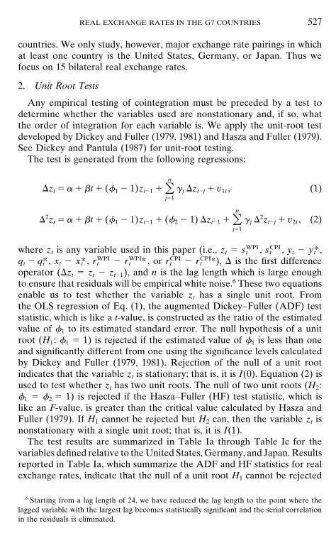
The test results are summarized in Table Ia through Table Ic for thevariables defined relative to the United States, Germany, and Japan. Resultsreported in Table Ia, which summarize the ADF and HF statistics for realexchange rates, indicate that the null of a unit root H1 cannot be rejected
6 Starting from a lag length of 24, we have reduced the lag length to the point where thelagged variable with the largest lag becomes statistically significant and the serial correlationin the residuals is eliminated.
528 KAWAI AND OHARA
TA
BL
EIa
RE
SU
LT
SO
FU
NIT
-RO
OT
TE
ST
S:
RE
AL
EX
CH
AN
GE
RA
TE
S
Tes
tfor
asi
ngle
unit
root
Tes
tfo
rdo
uble
unit
root
sA
ugm
ente
dD
icke
y–F
ulle
rte
stA
ugm
ente
dD
icke
y–F
ulle
rte
stH
asza
–Ful
ler
test
Bila
tera
lre
alex
chan
gera
teSa
mpl
epe
riod
No.
lags
f1
AD
FN
o.la
gsf
2A
DF
No.
lags
HF
(1)
WP
I-ba
sed
real
exch
ange
rate
sC
anad
ian
dolla
r/U
.S.
dolla
r19
73.1
0–19
96.0
518
0.97
22.
3612
0.27
23.
95**
177.
62F
renc
hfr
anc/
U.S
.dol
lar
1973
.10–
1996
.02
210.
982
1.96
200.
342
3.19
*20
7.30
Ger
man
mar
k/U
.S.
dolla
r19
73.1
0–19
94.1
221
0.98
21.
8716
0.29
23.
68**
206.
99It
alia
nlir
e/U
.S.d
olla
r19
73.1
0–19
93.1
121
0.97
22.
2116
0.32
23.
45**
205.
71Ja
pane
seye
n/U
.S.d
olla
r19
73.1
0–19
96.0
522
0.96
22.
4115
0.20
24.
15**
217.
93U
.K.p
ound
ster
ling/
U.S
.dol
lar
1978
.05–
1996
.02
210.
952
2.63
10.
232
9.73
**20
7.69
Can
adia
ndo
llar/
Ger
man
mar
k19
73.1
0–19
94.1
222
0.96
22.
4420
0.34
23.
14*
217.
01F
renc
hfr
anc/
Ger
man
mar
k19
73.1
0–19
94.1
29
0.95
23.
028
0.18
24.
56**
815
.46*
*It
alia
nlir
e/G
erm
anm
ark
1973
.10–
1993
.11
200.
902
2.97
180.
172
2.97
*19
7.60
Japa
nese
yen
/Ger
man
mar
k19
73.1
0–19
94.1
215
0.95
22.
5117
20.
262
5.73
**14
19.5
9**
U.K
.pou
ndst
erlin
g/G
erm
anm
ark
1978
.05–
1994
.12
190.
982
1.42
182
0.03
24.
34**
1811
.20*
Can
adia
ndo
llar/
Japa
nese
yen
1973
.10–
1996
.05
220.
942
3.17
120.
292
4.25
**21
9.50
*F
renc
hfr
anc/
Japa
nese
yen
1973
.10–
1996
.02
150.
952
2.43
140.
042
5.46
**14
18.6
6**
Ital
ian
lire/
Japa
nese
yen
1973
.10–
1993
.11
150.
952
2.34
140.
102
5.19
**14
16.4
6**
U.K
.pou
ndst
erlin
g/Ja
pane
seye
n19
78.0
5–19
96.0
224
0.92
22.
8721
0.06
23.
22*
237.
63
REAL EXCHANGE RATES IN THE G7 COUNTRIES 529
(2)
CP
I-ba
sed
real
exch
ange
rate
sC
anad
ian
dolla
r/U
.S.
dolla
r19
73.1
0–19
96.0
518
0.97
22.
4812
0.41
23.
59**
176.
41F
renc
hfr
anc/
U.S
.dol
lar
1973
.10–
1996
.02
220.
972
2.14
160.
292
3.98
**21
6.74
Ger
man
mar
k/U
.S.
dolla
r19
73.1
0–19
94.1
221
0.98
21.
7920
0.35
23.
10*
206.
54It
alia
nlir
e/U
.S.d
olla
r19
73.1
0–19
93.1
217
0.97
22.
1316
0.28
23.
75**
169.
43*
Japa
nese
yen
/U.S
.dol
lar
1973
.10–
1996
.05
220.
962
2.40
150.
252
4.20
**21
8.00
U.S
.pou
ndst
erlin
g/U
.S.
dolla
r19
78.0
5–19
96.0
221
0.96
22.
6617
0.32
22.
88*
206.
18C
anad
ian
dolla
r/G
erm
anm
ark
1973
.10–
1994
.12
220.
962
2.57
210.
482
2.56
216.
70F
renc
hfr
anc/
Ger
man
mar
k19
73.1
0–19
94.1
213
0.92
23.
89*
60.
262
5.91
**12
15.6
3**
Ital
ian
lire/
Ger
man
mar
k19
73.1
0–19
93.1
224
0.95
22.
1923
0.54
21.
5623
3.69
Japa
nese
yen
/Ger
man
mar
k19
73.1
0–19
94.1
215
0.95
22.
6014
20.
032
6.00
**14
21.8
8**
U.K
.pou
ndst
erlin
g/G
erm
anm
ark
1978
.05–
1994
.12
220.
972
1.93
00.
352
11.1
4**
216.
34C
anad
ian
dolla
r/Ja
pane
seye
n19
73.1
0–19
96.0
522
0.95
23.
1112
0.40
23.
86**
219.
44*
Fre
nch
fran
c/Ja
pane
seye
n19
73.1
0–19
96.0
219
0.94
22.
9018
0.15
24.
11**
1812
.99*
*It
alia
nlir
e/Ja
pane
seye
n19
73.1
0–19
93.1
224
0.92
23.
1014
0.13
25.
41**
239.
50*
U.K
.pou
ndst
erlin
g/Ja
pane
seye
n19
78.0
5–19
96.0
224
0.94
22.
9121
0.30
23.
08*
237.
58
Not
e.D
oubl
eas
teri
sks
(**)
and
asi
ngle
aste
risk
(*),
resp
ecti
vely
,in
dica
teth
atth
est
atis
tics
are
sign
ifica
ntat
the
1an
d5%
leve
ls.
530 KAWAI AND OHARA
TA
BL
EIb
RE
SU
LT
SO
FU
NIT
-RO
OT
TE
ST
S:
RA
TIO
SO
FL
AB
OR
PR
OD
UC
TIV
ITY
,T
ER
MS
OF
TR
AD
E,A
ND
RE
AL
TR
AD
EB
AL
AN
CE
Tes
tfor
asi
ngle
unit
root
Tes
tfo
rdo
uble
unit
root
sA
ugm
ente
dD
icke
y–F
ulle
rte
stA
ugm
ente
dD
icke
y–F
ulle
rte
stH
asza
–Ful
ler
test
Cou
ntry
pair
sSa
mpl
epe
riod
No.
lags
f1
AD
FN
o.la
gsf
2A
DF
No.
lags
HF
(1)
Rat
ios
ofla
bor
prod
ucti
vity
(ind
ustr
ial
prod
ucti
on/l
abor
empl
oym
ent)
Can
ada/
Uni
ted
Stat
es19
73.1
0–19
96.0
524
0.87
23.
4019
20.
442
3.82
**23
9.88
*F
ranc
e/U
nite
dSt
ates
1973
.10–
1996
.02
220.
882
2.33
212
2.42
25.
93**
2120
.82*
*G
erm
any/
Uni
ted
Stat
es19
73.1
0–19
94.1
28
0.90
22.
4516
21.
332
4.31
**7
22.1
0**
Ital
y/U
nite
dSt
ates
1973
.10–
1993
.11
240.
912
1.53
232
1.70
23.
96**
2310
.14*
*Ja
pan
/Uni
ted
Stat
es19
73.1
0–19
96.0
522
0.97
22.
0921
0.03
23.
44*
219.
98*
Uni
ted
Kin
gdom
/Uni
ted
Stat
es19
78.0
5–19
96.0
216
0.84
23.
2313
20.
512
4.41
**15
11.2
9*C
anad
a/G
erm
any
1973
.10–
1994
.12
130.
892
2.61
112
1.07
25.
28**
1213
.73*
*F
ranc
e/G
erm
any
1973
.10–
1994
.12
220.
882
1.71
212
2.25
24.
40**
2110
.47*
Ital
y/G
erm
any
1973
.10–
1993
.11
240.
922
1.25
232
2.17
24.
20**
239.
55*
Japa
n/G
erm
any
1973
.10–
1994
.12
230.
982
0.59
212
0.22
22.
7422
5.39
Uni
ted
Kin
gdom
/Ger
man
y19
78.0
5–19
94.1
216
0.86
22.
661
20.
772
14.8
1**
156.
99C
anad
a/Ja
pan
1973
.10–
1996
.05
230.
942
3.26
220.
212
2.50
228.
79F
ranc
e/Ja
pan
1973
.10–
1996
.02
220.
962
2.17
210.
022
2.43
215.
65It
aly/
Japa
n19
73.1
0–19
93.1
124
0.94
21.
0823
21.
502
3.25
*23
7.45
Uni
ted
Kin
gdom
/Jap
an19
78.0
5–19
96.0
223
0.92
23.
1121
0.09
23.
11*
229.
03
(2)
Rat
ios
ofte
rms
oftr
ade
(exp
ort
pric
e/im
port
pric
e)C
anad
a/U
nite
dSt
ates
1973
.10–
1996
.05
220.
942
2.41
232
0.24
23.
96**
219.
34*
Fra
nce/
Uni
ted
Stat
es19
73.1
0–19
96.0
22
0.94
22.
3518
20.
782
4.63
**1
119.
90**
Ger
man
y/U
nite
dSt
ates
1973
.10–
1994
.12
240.
942
2.13
232
0.43
23.
40*
238.
13It
aly/
Uni
ted
Stat
es19
73.1
0–19
93.1
113
0.93
22.
7617
20.
502
4.16
**12
10.0
1*
REAL EXCHANGE RATES IN THE G7 COUNTRIES 531Ja
pan
/Uni
ted
Stat
es19
73.1
0–19
96.0
520
0.96
22.
4513
0.34
23.
62**
199.
21U
nite
dK
ingd
om/U
nite
dSt
ates
1978
.05–
1996
.02
120.
912
3.62
*14
0.04
24.
30**
1113
.72*
*C
anad
a/G
erm
any
1973
.10–
1994
.12
160.
922
2.77
152
0.40
25.
18**
1517
.62*
*F
ranc
e/G
erm
any
1973
.10–
1994
.12
230.
872
2.00
222
2.94
25.
19**
2215
.50*
*It
aly/
Ger
man
y19
73.1
0–19
93.1
113
0.79
23.
0316
22.
372
5.42
**12
19.2
5**
Japa
n/G
erm
any
1973
.10–
1994
.12
160.
962
1.92
152
0.02
25.
21**
1515
.95*
*U
nite
dK
ingd
om/G
erm
any
1978
.05–
1994
.12
190.
932
2.74
180.
222
2.73
187.
58C
anad
a/Ja
pan
1973
.10–
1996
.05
230.
952
2.81
220.
222
3.71
**22
10.8
6*F
ranc
e/Ja
pan
1973
.10–
1996
.02
200.
962
2.14
192
0.05
24.
45**
1911
.94*
*It
aly/
Japa
n19
73.1
0–19
93.1
124
0.95
22.
0823
20.
032
3.31
*23
8.38
Uni
ted
Kin
gdom
/Jap
an19
78.0
5–19
96.0
215
0.94
23.
1014
0.42
23.
75**
1411
.41*
(3)
Rat
ios
ofre
altr
ade
bala
nce
(exp
ort
quan
tity
/im
port
quan
tity
)C
anad
a/U
nite
dSt
ates
1973
.10–
1996
.05
220.
912
2.53
212
2.08
24.
83**
2116
.47*
*F
ranc
e/U
nite
dSt
ates
1973
.10–
1996
.02
150.
902
3.01
172
0.66
23.
43*
148.
53G
erm
any/
Uni
ted
Stat
es19
73.1
0–19
94.1
218
0.94
22.
2217
20.
572
3.50
**17
8.92
Ital
y/U
nite
dSt
ates
1973
.10–
1993
.11
210.
862
2.59
202
1.21
23.
29*
208.
86Ja
pan
/Uni
ted
Stat
es19
73.1
0–19
96.0
524
0.93
22.
3223
20.
342
2.89
*23
7.88
Uni
ted
Kin
gdom
/Uni
ted
Stat
es19
78.0
5–19
96.0
216
0.91
21.
9417
21.
702
3.63
**15
8.83
Can
ada/
Ger
man
y19
73.1
0–19
94.1
212
0.94
22.
3111
20.
212
3.53
**11
8.99
Fra
nce/
Ger
man
y19
73.1
0–19
94.1
219
0.93
22.
0318
20.
742
4.23
**18
11.0
9*It
aly/
Ger
man
y19
73.1
0–19
93.1
124
0.94
22.
3717
20.
242
3.20
*23
5.36
Japa
n/G
erm
any
1973
.10–
1994
.12
240.
932
2.27
232
0.47
22.
98*
237.
14U
nite
dK
ingd
om/G
erm
any
1978
.05–
1994
.12
240.
902
2.66
112
0.21
23.
42*
235.
76C
anad
a/Ja
pan
1973
.10–
1996
.05
240.
932
1.37
232
1.34
23.
80**
238.
71F
ranc
e/Ja
pan
1973
.10–
1996
.02
240.
922
1.54
232
1.29
23.
42*
238.
31It
aly/
Japa
n19
73.1
0–19
93.1
124
0.91
21.
9222
21.
762
3.79
**23
6.57
Uni
ted
Kin
gdom
/Jap
an19
78.0
5–19
96.0
223
0.96
20.
7922
21.
802
3.88
**22
9.19
Not
e.D
oubl
eas
teri
sks
(**)
and
asi
ngle
aste
risk
(*),
resp
ecti
vely
,in
dica
teth
atth
est
atis
tics
are
sign
ifica
ntat
the
1an
d5%
leve
ls.
532 KAWAI AND OHARA
TA
BL
EIc
RE
SU
LT
SO
FU
NIT
-RO
OT
TE
ST
S:
LO
NG
-TE
RM
RE
AL
INT
ER
ES
TR
AT
ED
IFF
ER
EN
TIA
LS
Tes
tfor
asi
ngle
unit
root
Tes
tfo
rdo
uble
unit
root
sA
ugm
ente
dD
icke
y–F
ulle
rte
stA
ugm
ente
dD
icke
y–F
ulle
rte
stH
asza
–Ful
ler
test
Cou
ntry
pair
sSa
mpl
epe
riod
No.
lags
f1
AD
FN
o.la
gsf
2A
DF
No.
lags
HF
(1)
WP
I-ba
sed
long
-ter
mre
alin
tere
stra
tedi
ffer
enti
als
Can
ada/
Uni
ted
Stat
es19
73.1
0–19
96.0
512
0.87
22.
8611
20.
992
5.33
**11
18.6
5**
Fra
nce/
Uni
ted
Stat
es19
73.1
0–19
96.0
223
0.83
22.
2422
22.
962
7.87
**22
33.9
9**
Ger
man
y/U
nite
dSt
ates
1973
.10–
1994
.12
220.
952
1.90
212
0.84
24.
42**
2112
.28*
*It
aly/
Uni
ted
Stat
es19
73.1
0–19
93.1
123
0.84
21.
8722
23.
462
6.31
**22
21.7
8**
Japa
n/U
nite
dSt
ates
1973
.10–
1996
.05
160.
792
3.70
*20
22.
202
6.20
**15
22.0
1**
Uni
ted
Kin
gdom
/Uni
ted
Stat
es19
78.0
5–19
96.0
213
0.83
23.
2113
21.
102
4.72
**12
13.8
9**
Can
ada/
Ger
man
y19
73.1
0–19
94.1
26
0.93
22.
295
20.
572
8.28
**5
38.6
5**
Fra
nce/
Ger
man
y19
73.1
0–19
94.1
223
0.80
22.
0922
23.
452
6.72
**22
25.9
8**
Ital
y/G
erm
any
1973
.10–
1993
.11
230.
882
2.10
222
2.94
25.
48**
2218
.33*
*Ja
pan
/Ger
man
y19
73.1
0–19
94.1
221
0.69
23.
2620
22.
502
5.92
**20
23.8
5**
Uni
ted
Kin
gdom
/Ger
man
y19
78.0
5–19
94.1
224
0.55
23.
2923
22.
932
4.10
**23
14.5
2**
Can
ada/
Japa
n19
73.1
0–19
96.0
521
0.84
22.
3020
22.
452
6.38
**20
23.3
1**
Fra
nce/
Japa
n19
73.1
0–19
96.0
223
0.70
22.
6822
23.
822
6.99
**22
28.7
2**
Ital
y/Ja
pan
1973
.10–
1993
.11
210.
852
1.83
202
3.87
25.
68**
2018
.04*
*U
nite
dK
ingd
om/J
apan
1978
.05–
1996
.02
170.
682
2.80
162
2.78
25.
33**
1619
.11*
*
REAL EXCHANGE RATES IN THE G7 COUNTRIES 533
(2)
CP
I-ba
sed
long
-ter
mre
alin
tere
stra
tedi
ffer
enti
als
Can
ada/
Uni
ted
Stat
es19
73.1
0–19
96.0
524
0.79
22.
7123
22.
232
3.94
**23
11.5
7*F
ranc
e/U
nite
dSt
ates
1973
.10–
1996
.02
240.
882
2.09
222
2.74
25.
53**
2313
.26*
*G
erm
any/
Uni
ted
Stat
es19
73.1
0–19
94.1
218
0.95
22.
0117
20.
512
4.13
**17
10.5
7*It
aly/
Uni
ted
Stat
es19
73.1
0–19
93.1
224
0.87
21.
8523
22.
512
4.78
**23
13.3
0**
Japa
n/U
nite
dSt
ates
1973
.10–
1996
.05
240.
912
2.00
232
1.57
24.
18**
2310
.75*
Uni
ted
Kin
gdom
/Uni
ted
Stat
es19
78.0
5–19
96.0
224
0.80
22.
8523
21.
342
3.15
*23
9.66
*C
anad
a/G
erm
any
1973
.10–
1994
.12
170.
892
2.71
182
1.20
24.
09**
1611
.99*
*F
ranc
e/G
erm
any
1973
.10–
1994
.12
240.
942
1.92
232
0.62
23.
42*
237.
87It
aly/
Ger
man
y19
73.1
0–19
93.1
224
0.88
22.
4123
21.
182
4.14
**23
11.7
0*Ja
pan
/Ger
man
y19
73.1
0–19
94.1
224
0.82
22.
8323
21.
932
5.06
**23
17.3
8**
Uni
ted
Kin
gdom
/Ger
man
y19
78.0
5–19
94.1
224
0.84
22.
8423
21.
782
4.01
**23
13.0
9**
Can
ada/
Japa
n19
73.1
0–19
96.0
524
0.82
22.
3223
22.
732
5.09
**23
15.5
6**
Fra
nce/
Japa
n19
73.1
0–19
96.0
224
0.90
21.
8523
22.
292
4.38
**23
11.2
1*It
aly/
Japa
n19
73.1
0–19
93.1
224
0.73
23.
1323
21.
802
4.16
**23
13.9
2**
Uni
ted
Kin
gdom
/Jap
an19
78.0
5–19
96.0
224
0.75
22.
7423
22.
782
4.19
**23
12.9
7**
Not
e.D
oubl
eas
teri
sks
(**)
and
asi
ngle
aste
risk
(*),
resp
ecti
vely
,in
dica
teth
atth
est
atis
tics
are
sign
ifica
ntat
the
1an
d5%
leve
ls.
534 KAWAI AND OHARA
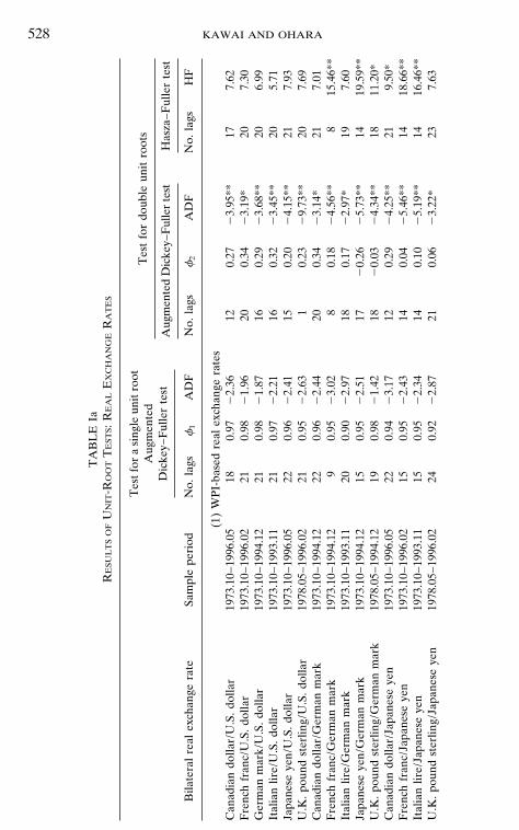
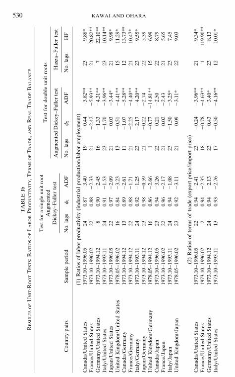
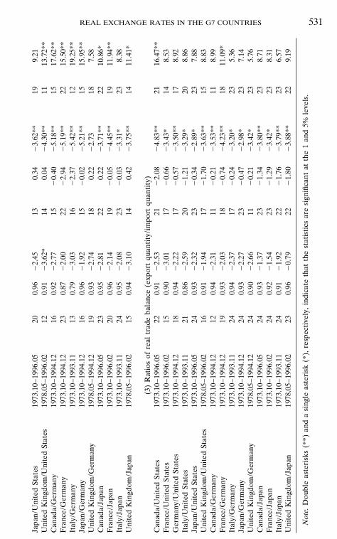
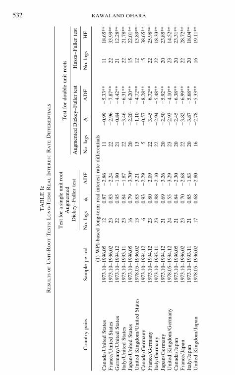
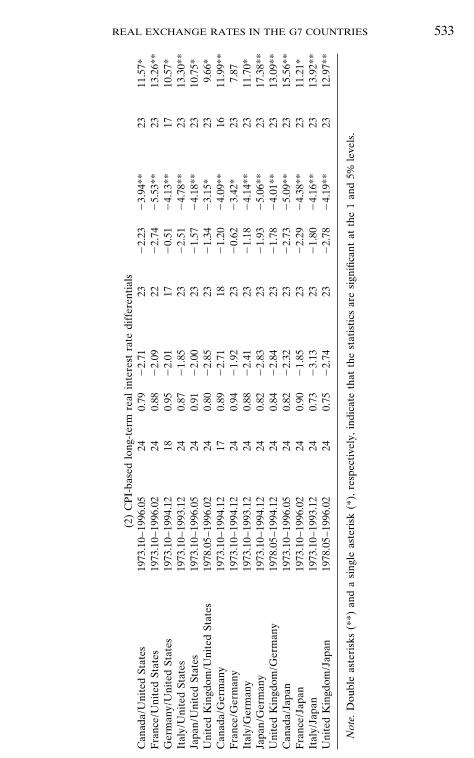
at the 5% level for any real exchange rate except for the French franc/German mark (CPI based). The null of two unit roots H2 can be rejectedfor all real exchange rates except for the Canadian dollar/German markand Italian lire/German mark pairings (CPI based), for which the presenceof two unit roots cannot be rejected.7 Similarly many other real economicvariables have single unit roots, as can be checked in Tables Ib and Ic.That is, they are I(1). A few variables, however, appear to be stationary,that is, they are I(0). In the Johansen or Johansen–Juselius approach, it isnot a serious problem for some variables to be stationary.
III. THE COINTEGRATION TESTING PROCEDURE
Procedures for evaluating long-run relationships between economic vari-ables have been developed within the framework of cointegration testingby Engle and Granger (1987), Engle and Yoo (1987), Johansen (1988, 1991,1995), Stock and Watson (1988), and Johansen and Juselius (1990).
The cointegration testing procedures attempt to examine the proposalthat deviations from equilibrium relationships for two or more variables,which are nonstationary when taken by themselves, are stationary as agroup. Despite the possibility of significant short-run deviations, economicforces may prohibit persistent long-run deviations from equilibrium rela-tionships. While individual economic variables such as real exchange rateswander extensively, certain groups of such variables may not diverge fromone another in the long run.
Cointegration tests provide an especially apt framework for evaluatinglong-run relationships between real exchange rates and a set of relevantreal economic variables. Real exchange rates have exhibited considerablevolatility since the advent of generalized floating exchange rates in the firsthalf of the 1970s. In the previous section, we found that most of the bilateralreal exchange rates for the G7 countries are nonstationary. However, long-run equilibrium may ensure that real exchange rates, despite being nonsta-tionary, do not wander arbitrarily far apart from other real and also nonsta-tionary economic variables and revert to equilibrium in the long run. Thus,it is of great interest to test if there exist cointegrating relationships betweenreal exchange rates and other relevant real economic variables. The pres-ence of cointegration would support the claim that real exchange rateshave long-run, stable relations to real factors in the economy that do notdiverge arbitrarily far from equilibrium.
7 In the tables, values corresponding to HF are the HF-statistics to test the null hypothesis(H2) that f1 5 f2 5 1. To save space, the tables do not report the estimated coefficients off1 when testing two unit roots.
REAL EXCHANGE RATES IN THE G7 COUNTRIES 535
1. The Johansen Multivariate Cointegration Approach
We use the multivariate maximum likelihood cointegration techniquedeveloped by Johansen (1988, 1991, 1995) and Johansen and Juselius(1992).8 Use of Johansen’s technique controls for endogeneity and compli-cated short-run dynamics and focuses on long-run relationships amongnonstationary variables. In comparison to the more popular Engle–Granger(1987) method, one of the biggest advantages of the Johansen approach isthat it can detect the presence of several cointegrating vectors. Although theEngle–Granger method has its own strong points, we utilize the Johansenmultivariate approach because of its capacity to discover more than onecointegrating relationship between the real exchange rate and other rele-vant real economic variables.9
The Johansen multivariate approach requires the use of test statistics toevaluate cointegrating relationships among a group of many variables.These test statistics have a limiting distribution that is a function of a singleparameter. This approach expresses the possible cointegrating relationshipsamong the p variables in X as a vector autoregression of order k, VAR(k),with Gaussian errors. Generally, the approach is applied to I(1) variables,but, as indicated earlier, it is not a serious problem for some variables tobe stationary. The p-dimensional VAR system to be estimated is:
Xt 5 e 1 CDt 1 F1Xt21 1 ? ? ? 1 FkXt2k 1 JHt 1 ut , t 5 1, . . ., T, (3)
where Xt is a p 3 T matrix of [st yt 2 y*t qt 2 q*t xt 2 x*t rt 2 r*t ], Ht
represent exogenous variables, Dt are centered seasonal dummies, and ut
are i.i.d. Np(0, V).By subtracting Xt21 from both sides of system (3) and rearranging the
right-hand side, we can rewrite the model in error correction form:
DXt 5 e 1 CDt 1 PXt21 1 G1 DXt21 1 ? ? ? 1 Gk21 DXt2k11 (4)1 j Dht 1 ut , t 5 1, . . ., T,
where P 5 F1 1 ? ? ? 1 Fk 2 I, and Gj 5 F1 1 ? ? ? 1 Fj 2 (I 1 P),j 5 1, 2, . . ., k 2 1. As in the case of Johansen and Juselius (1992), wehave added the log first difference of the world real oil price, Dht , to theright-hand side.10 The number of variables used for Xt is five, that is,
8 See Hamilton (1994, Chaps. 19–20) for a general treatment of cointegration and its testing.9 Performance evaluation of finite-sample cointegration tests is mixed; Inder (1993) con-
cluded that the Engle–Granger method involves large biases while Gregory (1994) favors theEngle–Granger method over the Johansen–Juselius method.
10 The world real oil price ht is defined as the natural log of the spot oil price in U.S. dollars(obtained from the IMF’s International Financial Statistics) deflated by U.S. WPI.
536 KAWAI AND OHARA
p 5 5. We have chosen the autoregressive order in model (4) to be 5, thatis, k 2 1 5 5. This order generally yields both low serial correlationsof the residuals and jointly significant final lags for the five variables ineach equation.
The rank of the coefficient matrix P gives the number of cointegratingvectors, r , p.11 If this rank is greater than zero the matrix P can berewritten as:
P 5 AB9, (5)
where A (alpha) is the p 3 r matrix of adjustment coefficients and B (beta)is the p 3 r matrix of cointegrating vectors. This expression is tantamountto the hypothesis that the rank of P is reduced to a value r , p. This impliesthat the first differenced process DXt is stationary, Xt is nonstationary, andB9Xt is stationary. Thus, we can interpret the linear combinations B9Xt asrepresenting stationary relations among the nonstationary variables whichinclude the real exchange rate and other real economic variables; theirlinear combinations constitute the cointegrating relationships.
2. Likelihood Ratio Tests
Johansen and Juselius (1990, 1992) presented several likelihood ratiotests to determine the number of cointegrating vectors in Xt . Known asthe trace test, the first test evaluates the null hypothesis that there are ror fewer cointegrating vectors against the alternative that there are morethan r. The trace test statistic is given by
ttrace(r) 5 2T Opj5r11
ln(1 2 lj), (6)
where lr11, . . ., lp denote the p 2 r smallest squared canonical correlationsbetween the first differences and the levels of the variables, with dynamicand deterministic factors factored out.12 Known as the maximal-eigenvalue
11 The impact coefficient matrix P contains all long-run information. Three possibilitiesexist: (a) the matrix P has full column rank p, implying that Xt is stationary to begin with;(b) the matrix P has zero rank, implying that the system of Eqs. (4) is a traditional first-differenced VAR; and (c) the rank of P is r and smaller than p, implying that there exist rlinear combinations of Xt that are stationary or cointegrated.
12 To obtain the lj , we estimate the following models:
DXt 5 Om21
j51U0j DXt2j 1 w0t , Xt21 5 Om21
j51U1j DXt2j 1 w1t .
The residual vectors w0t and w1t are used to calculate the squared canonical correlations.
REAL EXCHANGE RATES IN THE G7 COUNTRIES 537
test, the second likelihood ratio test evaluates the null that there are exactlyr cointegrating vectors in Xt against the alternative that there are r 1 1.The maximal-eigenvalue test statistic is given by
lmax(r) 5 ttrace(r) 2 ttrace(r 1 1) 5 2T ln(1 2 lr11). (7)
Asymptotic critical values corrected for degrees of freedom for these twotest statistics are given by Reimers (1992). Of these two likelihood ratiotests, Johansen and Juselius (1990) suggest that the trace test may lackpower relative to the maximal eigenvalue test.
Johansen and Juselius (1990) also present a likelihood ratio test forconstraints applied to the matrices A (alpha) and B (beta). The constraintsapply equally to all vectors. The asymptotically x2 statistic is given by
LRcon 5 2T Or
j51ln[(1 2 lcon, j)/(1 2 lj)], (8)
where lcon, j are obtained from the constrained estimation, and r is thenumber of cointegrating vectors already assumed.
Finally, for cases of more than one cointegrating vector, Johansen andJuselius present a test for constraints on a subset of the vectors. We focuson their hypothesis H6 (Johansen and Juselius (1992, pp. 225, 233–236))as a relevant set of constraints. The asymptotically x2 test statistic is
LRH6 5 2T FOr1
j51ln(1 2 l1,H6, j) 1 Or2
j51ln(1 2 l2,H6, j)
(9)
2 Or
j51ln(1 2 lj) G ,
where l1,H6, j and l2,H6, j are obtained from the constrained estimation, r1 isthe number of vectors to be constrained, and r2 5 r 2 r1.
IV. EMPIRICAL TESTING OF COINTEGRATINGRELATIONSHIPS
1. Testing for Reduced Rank
To determine the number of cointegrating vectors, we perform two likeli-hood ratio tests by examining the trace test statistic, ttrace(r), and the maxi-mal-eigenvalue test statistic, lmax(r). These test results are reported inTable II, where asterisks are attached to statistically significant results afteradjustment for degrees of freedom.
538 KAWAI AND OHARA
Table IIa reports the ttrace and lmax test statistics for each country pairwhen WPI-based real exchange rates are used. Table IIb reports the samefor CPI-based real exchange rates.13 Results reported in Table IIa indicatethat the null hypothesis of no cointegration is rejected, at the standard 5%level of significance, in all cases except for the country pairs Italy/Germanyand Italy/Japan. The null of no cointegration is barely rejected for Canada/Germany. The null hypothesis of one cointegrating vector cannot be re-jected for the country pairs Canada/United States, Germany/United States,Italy/United States, Canada/Germany, France/Germany, Japan/Germany,or Canada/Japan, suggesting that each of these country pairs has one cointe-grating relationship among the real economic variables based on the WPI-based real exchange rate. The null hypothesis of one cointegrating vectoris rejected but the null of two cointegrating vectors is not rejected for thecountry pairs Japan/United States and France/Japan. The null of threecointegrating vectors cannot be rejected for United Kingdom/United Statesor United Kingdom/Japan. For these groups of country pairs, there areone or more cointegrating relationships. Though it is not clear whether thenumber of cointegrating vectors is one or greater for France/United States,we conclude that this pair has only one cointegrating vector based on theresults of the maximal eigenvalue test statistics (lmax).
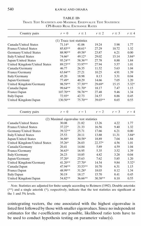
Turning to Table IIb where results for CPI-based real exchange ratesare summarized, the null hypothesis of no cointegration is rejected in allcases except for the country pairs Canada/Germany and Italy/Germany.Rejection of no cointegration for Italy/Japan and France/Germany is basedrespectively on trace test statistics (ttrace) and maximal eigenvalue teststatistics (lmax). The null of one cointegrating vector cannot be rejected forCanada/United States, France/Germany, Japan/Germany, or Italy/Japan.The null of two cointegrating vectors cannot be rejected for France/UnitedStates, Germany/United States, Italy/United States, Japan/United States,United Kingdom/United States, Canada/Japan, or France/Japan, and thenull of three cointegrating vectors cannot be rejected for United Kingdom/Germany or United Kingdom/Japan. Some of these conclusions are basedon trace test statistics (ttrace).
These results are consistent with the proposition that the real economicvariables, including the WPI- or CPI-based real exchange rate, of most ofthe G7 country pairs are cointegrated with one another.
2. Tests of Zero Restrictions on the Real Exchange Rate in theCointegrating Vectors
Table III gives the estimated cointegrating vector (or vectors) for eachcountry pair where we have concluded the existence of cointegration atthe 5% significance level, using trace or maximal eigenvalue test statistics.
13 Note that when the WPI-based real exchange rate is used as one of the Xt variables, theWPI-based long-term real interest rate differential is used. Similarly use of the CPI-basedreal exchange rate is accompanied by use of the CPI-based real interest rate differential.
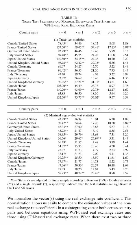
REAL EXCHANGE RATES IN THE G7 COUNTRIES 539
TABLE IIaTRACE TEST STATISTICS AND MAXIMAL EIGENVALUE TEST STATISTICS:
WPI-BASED REAL EXCHANGE RATES
Country pairs r 5 0 r # 1 r # 2 r # 3 r # 4
(1) Trace test statisticsCanada/United States 78.45** 34.46 18.12 8.08 1.88France/United States 157.50** 59.05** 34.41* 17.15* 6.87**Germany/United States 92.79** 46.46 19.46 5.79 0.13Italy/United States 89.48** 45.75 24.28 11.08 2.54Japan/United States 110.80** 54.15** 24.36 10.70 3.20United Kingdon/United States 98.98** 62.42** 32.75* 6.76 1.44Canada/Germany 61.07 24.27 12.70 5.22 1.44France/Germany 91.42** 36.55 21.20 7.73 3.44Italy/Germany 47.70 19.74 8.01 3.22 0.99Japan/Germany 73.87* 36.69 15.46 6.46 1.36United Kingdom/Germany 96.95** 57.21** 31.71* 13.21 1.60Canada/Japan 103.20** 45.49 23.72 8.97 0.75France/Japan 110.20** 63.09** 32.73* 12.17 1.69Italy/Japan 65.83 36.50 18.30 5.64 0.20United Kingdom/Japan 132.50** 73.75** 33.02* 9.57 0.59
Country pairs r 5 0 r 5 1 r 5 2 r 5 3 r 5 4
(2) Maximal eigenvalue test statisticsCanada/United States 43.99** 16.34 10.04 6.20 1.88France/United States 98.42** 24.64 17.26 10.28 6.87**Germany/United States 46.33** 27.00 13.67 5.67 0.13Italy/United States 43.73** 21.47 13.19 8.55 2.54Japan/United States 56.65** 29.79* 13.66 7.51 3.20United Kingdom/United States 36.56* 29.67* 25.99** 5.31 1.44Canada/Germany 36.79* 11.57 7.48 3.79 1.44France/Germany 54.87** 15.35 13.46 4.30 3.44Italy/Germany 27.97 11.73 4.79 2.23 0.99Japan/Germany 37.17* 21.23 9.00 5.11 1.36United Kingdom/Germany 39.75** 25.50 18.50 11.61 1.60Canada/Japan 57.67** 21.77 14.75 8.22 0.75France/Japan 47.06** 30.36* 20.57 10.48 1.69Italy/Japan 29.33 18.20 12.67 5.43 0.20United Kingdom/Japan 58.73** 40.72** 23.45* 8.98 0.59
Note. Statistics are adjusted for finite sample according to Reimers (1992). Double asterisks(**) and a single asterisk (*), respectively, indicate that the test statistics are significant atthe 1 and 5% levels.
We normalize the vector(s) using the real exchange rate coefficient. Thisnormalization allows us easily to compare the estimated values of the non-real exchange rate coefficients in a cointegrating vector both across countrypairs and between equations using WPI-based real exchange rates andthose using CPI-based real exchange rates. When there exist two or three
540 KAWAI AND OHARA
TABLE IIbTRACE TEST STATISTICS AND MAXIMAL EIGENVALUE TEST STATISTICS:
CPI-BASED REAL EXCHANGE RATES
Country pairs r 5 0 r # 1 r # 2 r # 3 r # 4
(1) Trace test statisticsCanada/United States 71.14* 41.06 19.24 5.98 1.77France/United States 85.83** 48.61* 27.29 10.72 1.32Germany/United States 88.90** 49.58* 23.87 6.21 0.00Italy/United States 74.66* 49.12* 29.02 15.14 3.84*Japan/United States 95.24** 58.36** 27.78 8.88 1.84United Kingdom/United States 89.23** 53.97** 27.94 5.57 1.01Canada/Germany 46.77 26.35 11.52 5.63 1.04France/Germany 63.84** 27.21 10.25 4.91 1.39Italy/Germany 45.20 18.98 8.13 3.31 0.04Japan/Germany 77.49* 40.29 14.66 7.05 1.20United Kingdom/Germany 98.59** 57.39** 29.69* 15.15 5.32*Canada/Japan 99.64** 51.70* 18.17 7.47 1.15France/Japan 107.70** 58.76** 27.48 9.46 1.34Italy/Japan 72.93* 42.73 24.57 8.86 0.45United Kingdom/Japan 130.50** 75.70** 39.03** 8.65 0.55
Country pairs r 5 0 r 5 1 r 5 2 r 5 3 r 5 4
(2) Maximal eigenvalue test statisticsCanada/United States 30.08 21.82 13.26 4.22 1.77France/United States 37.22* 21.33 16.56 9.40 1.32Germany/United States 39.32** 25.71 17.66 6.21 0.00Italy/United States 25.53 20.11 13.88 11.31 3.84*Japan/United States 36.88* 30.58* 18.89 7.04 1.84United Kingdom/United States 35.26* 26.03 22.37* 4.56 1.01Canada/Germany 20.41 14.84 5.89 4.59 1.04France/Germany 36.63* 16.95 5.35 3.52 1.39Italy/Germany 26.23 10.85 4.82 3.28 0.04Japan/Germany 37.20* 25.63 7.62 5.85 1.20United Kingdom/Germany 41.20** 27.70* 14.54 9.84 5.32*Canada/Japan 47.94** 33.53** 10.70 6.31 1.15France/Japan 48.99** 31.28* 18.03 8.12 1.34Italy/Japan 30.19 18.17 15.70 8.41 0.45United Kingdom/Japan 54.82** 36.66** 30.38** 8.10 0.55
Note. Statistics are adjusted for finite sample according to Reimers (1992). Double asterisks(**) and a single asterisk (*), respectively, indicate that the test statistics are significant atthe 1 and 5% levels.
cointegrating vectors, the one associated with the highest eigenvalue islisted first followed by those with smaller eigenvalues. Since no independentestimates for the t-coefficients are possible, likelihood ratio tests have tobe used to conduct hypothesis testing on parameter value(s).
REAL EXCHANGE RATES IN THE G7 COUNTRIES 541
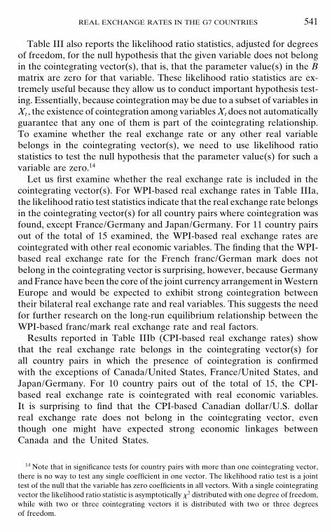
Table III also reports the likelihood ratio statistics, adjusted for degreesof freedom, for the null hypothesis that the given variable does not belongin the cointegrating vector(s), that is, that the parameter value(s) in the Bmatrix are zero for that variable. These likelihood ratio statistics are ex-tremely useful because they allow us to conduct important hypothesis test-ing. Essentially, because cointegration may be due to a subset of variables inXt , the existence of cointegration among variables Xt does not automaticallyguarantee that any one of them is part of the cointegrating relationship.To examine whether the real exchange rate or any other real variablebelongs in the cointegrating vector(s), we need to use likelihood ratiostatistics to test the null hypothesis that the parameter value(s) for such avariable are zero.14
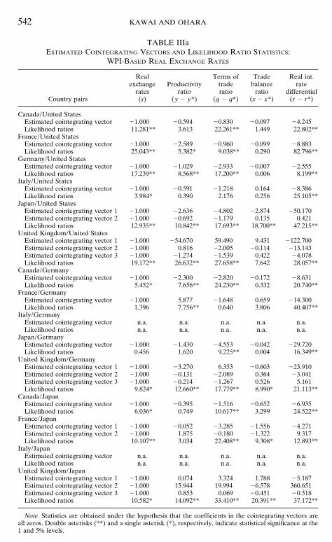
Let us first examine whether the real exchange rate is included in thecointegrating vector(s). For WPI-based real exchange rates in Table IIIa,the likelihood ratio test statistics indicate that the real exchange rate belongsin the cointegrating vector(s) for all country pairs where cointegration wasfound, except France/Germany and Japan/Germany. For 11 country pairsout of the total of 15 examined, the WPI-based real exchange rates arecointegrated with other real economic variables. The finding that the WPI-based real exchange rate for the French franc/German mark does notbelong in the cointegrating vector is surprising, however, because Germanyand France have been the core of the joint currency arrangement in WesternEurope and would be expected to exhibit strong cointegration betweentheir bilateral real exchange rate and real variables. This suggests the needfor further research on the long-run equilibrium relationship between theWPI-based franc/mark real exchange rate and real factors.
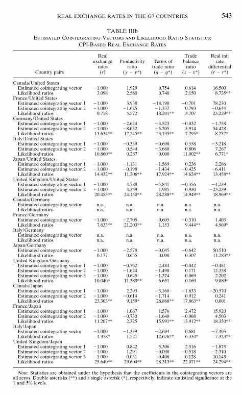
Results reported in Table IIIb (CPI-based real exchange rates) showthat the real exchange rate belongs in the cointegrating vector(s) forall country pairs in which the presence of cointegration is confirmedwith the exceptions of Canada/United States, France/United States, andJapan/Germany. For 10 country pairs out of the total of 15, the CPI-based real exchange rate is cointegrated with real economic variables.It is surprising to find that the CPI-based Canadian dollar/U.S. dollarreal exchange rate does not belong in the cointegrating vector, eventhough one might have expected strong economic linkages betweenCanada and the United States.
14 Note that in significance tests for country pairs with more than one cointegrating vector,there is no way to test any single coefficient in one vector. The likelihood ratio test is a jointtest of the null that the variable has zero coefficients in all vectors. With a single cointegratingvector the likelihood ratio statistic is asymptotically x2 distributed with one degree of freedom,while with two or three cointegrating vectors it is distributed with two or three degreesof freedom.
542 KAWAI AND OHARA
TABLE IIIaESTIMATED COINTEGRATING VECTORS AND LIKELIHOOD RATIO STATISTICS:
WPI-BASED REAL EXCHANGE RATES
Real Terms of Trade Real int.exchange Productivity trade balance rate
rates ratio ratio ratio differentialCountry pairs (s) (y 2 y*) (q 2 q*) (x 2 x*) (r 2 r*)
Canada/United StatesEstimated cointegrating vector 21.000 20.594 20.830 20.097 24.245Likelihood ratios 11.281** 3.613 22.261** 1.449 22.802**
France/United StatesEstimated cointegrating vector 21.000 22.589 20.960 20.099 28.883Likelihood ratios 25.043** 5.382* 9.038** 0.290 82.796**
Germany/United StatesEstimated cointegrating vector 21.000 21.029 22.933 20.007 22.555Likelihood ratios 17.239** 8.568** 17.200** 0.006 8.199**
Italy/United StatesEstimated cointegrating vector 21.000 20.591 21.218 0.164 28.386Likelihood ratios 3.984* 0.390 2.176 0.256 25.105**
Japan/United StatesEstimated cointegrating vector 1 21.000 22.636 24.802 22.874 250.170Estimated cointegrating vector 2 21.000 20.692 21.179 0.135 0.421Likelihood ratios 12.935** 10.842** 17.693** 18.700** 47.215**
United Kingdom/United StatesEstimated cointegrating vector 1 21.000 254.670 59.490 9.431 2122.700Estimated cointegrating vector 2 21.000 0.816 22.005 20.114 213.143Estimated cointegrating vector 3 21.000 21.274 21.539 0.422 24.078Likelihood ratios 19.172** 26.632** 27.658** 7.642 28.057**
Canada/GermanyEstimated cointegrating vector 21.000 22.300 22.820 20.172 28.631Likelihood ratios 5.452* 7.656** 24.230** 0.332 20.740**
France/GermanyEstimated cointegrating vector 21.000 5.877 21.648 0.659 214.300Likelihood ratios 1.396 7.756** 0.640 3.806 40.407**
Italy/GermanyEstimated cointegrating vector n.a. n.a. n.a. n.a. n.a.Likelihood ratios n.a. n.a. n.a. n.a. n.a.
Japan/GermanyEstimated cointegrating vector 21.000 21.430 24.553 20.042 229.720Likelihood ratios 0.456 1.620 9.225** 0.004 16.349**
United Kingdom/GermanyEstimated cointegrating vector 1 21.000 23.270 6.353 20.603 223.910Estimated cointegrating vector 2 21.000 20.131 22.089 0.364 23.041Estimated cointegrating vector 3 21.000 20.214 21.267 0.526 5.161Likelihood ratios 9.824* 12.660** 17.779** 8.990* 21.113**
Canada/JapanEstimated cointegrating vector 21.000 20.395 21.516 20.652 26.935Likelihood ratios 6.036* 0.749 10.617** 3.299 24.522**
France/JapanEstimated cointegrating vector 1 21.000 20.052 23.285 21.556 24.271Estimated cointegrating vector 2 21.000 1.875 20.180 21.322 9.317Likelihood ratios 10.107** 3.034 22.408** 9.308* 12.893**
Italy/JapanEstimated cointegrating vector n.a. n.a. n.a. n.a. n.a.Likelihood ratios n.a. n.a. n.a. n.a. n.a.
United Kingdom/JapanEstimated cointegrating vector 1 21.000 0.074 3.324 1.788 25.187Estimated cointegrating vector 2 21.000 15.944 19.994 26.578 360.651Estimated cointegrating vector 3 21.000 0.853 0.069 20.451 20.518Likelihood ratios 10.582* 14.092** 33.410** 20.391** 37.172**
Note. Statistics are obtained under the hypothesis that the coefficients in the cointegrating vectors areall zeros. Double asterisks (**) and a single asterisk (*), respectively, indicate statistical significance at the1 and 5% levels.
REAL EXCHANGE RATES IN THE G7 COUNTRIES 543
TABLE IIIbESTIMATED COINTEGRATING VECTORS AND LIKELIHOOD RATIO STATISTICS:
CPI-BASED REAL EXCHANGE RATES
Real Trade Real int.exchange Productivity Terms of balance rate
rates ratio trade ratio ratio differentialCountry pairs (s) (y 2 y*) (q 2 q*) (x 2 x*) (r 2 r*)
Canada/United StatesEstimated cointegrating vector 21.000 1.929 0.754 0.614 16.500Likelihood ratios 3.098 2.580 0.740 2.150 8.735**
France/United StatesEstimated cointegrating vector 1 21.000 3.938 218.190 20.701 78.230Estimated cointegrating vector 2 21.000 21.625 21.337 0.793 20.644Likelihood ratios 0.718 5.572 18.201** 3.707 23.229**
Germany/United StatesEstimated cointegrating vector 1 21.000 22.624 23.523 20.032 21.758Estimated cointegrating vector 2 21.000 28.052 25.205 5.914 54.428Likelihood ratios 13.634** 17.245** 23.195** 7.295* 8.257*
Italy/United StatesEstimated cointegrating vector 1 21.000 20.339 20.698 0.558 23.218Estimated cointegrating vector 2 21.000 0.544 23.680 0.806 7.267Likelihood ratios 10.860** 0.287 0.000 11.002** 6.771*
Japan/United StatesEstimated cointegrating vector 1 21.000 21.131 21.569 0.236 2.286Estimated cointegrating vector 2 21.000 20.198 21.434 20.425 26.411Likelihood ratios 14.432** 11.206** 17.924** 14.624** 13.458**
United Kingdom/United StatesEstimated cointegrating vector 1 21.000 4.788 25.841 20.356 24.239Estimated cointegrating vector 2 21.000 4.359 1.985 0.930 223.239Likelihood ratios 20.453** 24.150** 28.288** 14.949** 18.969**
Canada/GermanyEstimated cointegrating vector n.a. n.a. n.a. n.a. n.a.Likelihood ratios n.a. n.a. n.a. n.a. n.a.
France/GermanyEstimated cointegrating vector 21.000 22.705 0.605 20.310 1.403Likelihood ratios 7.633** 21.203** 1.153 9.444** 4.969*
Italy/GermanyEstimated cointegrating vector n.a. n.a. n.a. n.a. n.a.Likelihood ratios n.a. n.a. n.a. n.a. n.a.
Japan/GermanyEstimated cointegrating vector 21.000 22.578 20.045 20.642 50.510Likelihood ratios 0.177 0.655 0.000 0.307 11.283**
United Kingdom/GermanyEstimated cointegrating vector 1 21.000 20.762 2.484 20.042 20.481Estimated cointegrating vector 2 21.000 21.624 21.498 0.171 12.338Estimated cointegrating vector 3 21.000 0.645 21.374 0.069 2.202Likelihood ratios 10.040* 11.389** 6.651 0.169 9.889*
Canada/JapanEstimated cointegrating vector 1 21.000 2.293 23.160 21.633 220.570Estimated cointegrating vector 2 21.000 20.614 21.714 0.912 0.241Likelihood ratios 23.303** 9.159* 28.868** 17.863** 0.001
France/JapanEstimated cointegrating vector 1 21.000 21.067 1.576 2.472 15.920Estimated cointegrating vector 2 21.000 20.730 21.640 20.068 4.503Likelihood ratios 11.207** 2.325 15.991** 13.912** 18.350**
Italy/JapanEstimated cointegrating vector 21.000 21.339 22.694 0.681 27.403Likelihood ratios 4.378* 1.521 12.676** 6.334* 7.323**
United Kingdom/JapanEstimated cointegrating vector 1 21.000 0.842 5.306 2.516 21.875Estimated cointegrating vector 2 21.000 1.291 20.090 20.518 22.310Estimated cointegrating vector 3 21.000 20.031 20.408 20.128 10.143Likelihood ratios 25.640** 29.604** 28.313** 22.071** 24.294**
Note. Statistics are obtained under the hypothesis that the coefficients in the cointegrating vectors areall zeros. Double asterisks (**) and a single asterisk (*), respectively, indicate statistical significance at the1 and 5% levels.
544 KAWAI AND OHARA
3. Tests of Zero Restrictions on the Nonexchange Rate Variables
Next, we can examine whether a certain real variable other than the realexchange rate belongs in the cointegrating vector(s) with the correct sign.This allows us to test hypotheses concerning the presence of labor productiv-ity ratios, terms-of-trade ratios, real trade balance ratios, and long-termreal interest rate differentials in the cointegrating vector(s) in which thereal exchange rate belongs. The most notable example would be a test ofthe Balassa–Samuelson productivity-bias hypothesis.
The time series version of the Balassa–Samuelson hypothesis is that theparameter value(s) in the B matrix for the labor productivity ratio aresignificantly negative; the real exchange rate and the productivity ratio arenegatively correlated with each other in the long run. This is undoubtedlya simplified version of the Balassa–Samuelson hypothesis in that we abstractfrom interactions between the tradables and nontradables sectors and thedifferential productivity growth between these two sectors and across coun-tries. The likelihood ratio test statistics for the productivity ratio, reportedin Table IIIa, indicate that its coefficient(s) are significantly negative for 6country pairs out of the total of 11 for which the WPI-based real exchangerate was found to belong to the cointegrating vector(s). For only 1 pair,United Kingdom/Japan, are the coefficient(s) of the productivity ratio sig-nificantly positive, thus clearly contradicting the Balassa–Samuelson hy-pothesis. The likelihood ratio statistics reported in Table IIIb indicate thatthe coefficient(s) of the productivity ratio are significantly negative for 5country pairs out of the total of 10 for which the CPI-based real exchangerate was found to be part of the cointegrating vector(s). The Balassa–Samuelson hypothesis is rejected for only two pairs, United Kingdom/United States and United Kingdom/Japan. Hence we can conclude thatthe Balassa–Samuelson productivity-bias hypothesis holds for more thanhalf of the country pairs for which the real exchange rate belongs in thecointegrating vector(s).
Similarly, one can check whether the terms-of-trade ratio, the real tradebalance ratio, and the long-term real interest rate differential have signifi-cant coefficients in the cointegrating vector(s). Focusing on the 11 countrypairs for which the WPI-based real exchange rate is part of the cointegratingvector(s), 10 pairs exhibit significant coefficients for the terms-of-trade ratio,4 pairs for the trade balance ratio, and all 11 pairs for the long-term realinterest rate differential. Out of the 10 country pairs that show cointegrationusing CPI-based real exchange rates, 7 pairs exhibit significant coefficientsfor the terms-of-trade ratio, 9 pairs for the trade balance ratio, and 9 pairsfor the long-term real interest rate differential.
All in all, the results support the proposition that the bilateral real ex-
REAL EXCHANGE RATES IN THE G7 COUNTRIES 545
change rates for many G7 country pairs are cointegrated with a set of realeconomic variables, though there are some important exceptions such asFrance/Germany (WPI-based) and Canada/United States (CPI-based).Real economic variables, such as national labor productivity, the terms oftrade, the real trade balance, and the real interest rate differential, alsoplay significant roles in cointegrating vectors.
V. CONCLUDING REMARKS
Although not discussed in the text, we have conducted cointegrationtests using the real exchange rate and a set of nominal variables, such asthe relative money supply ratio and the long-term nominal interest ratedifferential. We have then confirmed that the real exchange rate is notcointegrated with these nominal variables, which supports the premise thatthe real exchange rate does not have a long-run stable relationship withnominal variables. This suggests that the movements in real exchange ratesare driven by changes in real variables, at least in the long run.
This paper has indeed found that the real exchange rates for many G7country pairs are cointegrated with real economic variables, such as laborproductivity, the terms of trade, real trade balances, and long-term realinterest rate differentials. The productivity variable is found to be statisti-cally significant with the correct sign for more than half of the country pairsfor which the real exchange rate belongs in the cointegrating vector(s).This lends support to the Balassa–Samuelson productivity-bias hypothesis.Other real variables are also found to have statistically significant coeffi-cients in many cases.
However, we have not been able to find any cointegrating vector for Italy/Germany (WPI and CPI based), Italy/Japan (WPI based), and Canada/Germany (CPI based). Even when a cointegrating vector is found to exist,we have not been able to confirm that the real exchange rate belongs inthe cointegrating vector for France/Germany (WPI based) and Canada/United States (CPI based). This puzzling result requires a deeper investiga-tion to discover a long-run equilibrium relationship between the bilateralreal exchange rate and real economic factors for the country pairs whichare generally considered to be well integrated.
The paper has covered only the post-Bretton Woods period for the G7countries. It would be useful to expand our analysis by including the fixedexchange rate period. Analysis of many other exchange rates and currencieswould also add knowledge and understanding of the behavior of real ex-change rates.
546 KAWAI AND OHARA
REFERENCES
Adler, Michael and Lehman, Bruce (1983). Deviations from purchasing power parity in thelong run, J. Fin. 38, 1471–1487.
Bahmani-Oskooee, Mohsen, and Rhee, Hyun-Jae (1996).Time-series support for Balassa’sproductivity-bias hypothesis: Evidence from Korea, Rev. Int. Econ. 4, 364–370.
Baillie, Richard T., and Selover, David D. (1987). Cointegration and models of exchange ratedetermination, Int. J. Forecasting 3, 43–51.
Balassa, Bela (1964). The purchasing power parity doctrine: A reappraisal, J. Polit. Econ.72, 584–596.
Boucher, Janice L. (1993). Tests of long-run purchasing power parity using alternative method-ologies, J. Macroecon. 15, 109–122.
Ceglowski, Janet (1996). The real yen exchange rate and Japanese productivity growth, Rev.Int. Econ. 4, 54–63.
Clarida, Richard, and Gali, Jordi (1994). Sources of real exchange rate fluctuations: Howimportant are nominal shocks?, Carnegie–Rochester Conf. Ser. Public Policy 41, 1–56.
Corbae, Dean, and Ouliaris, Sam (1988). Cointegration and tests of purchasing power parity,Rev. Econ. Statist. 70, 508–511.
Crowder, William J. (1996). A reexamination of long-run PPP: The case of Canada, the UK,and the US, Rev. Int. Econ. 4, 64–78.
Dickey, David A., and Fuller, Wayne A. (1979). Distribution of the estimators for autoregres-sive time series with a unit root, J. Amer. Statist. Assoc. 74, 427–431.
Dickey, David A., and Fuller, Wayne A. (1981). Likelihood ratio statistics for autoregressivetime series with a unit root, Econometrica 49, 1057–1072.
Dickey, David A., and Pantula, Sastry G. (1987). Determining the order of differencing inautoregressive processes, J. Bus. Econ. Statis. 5, 455–461.
Edison, Hali J. (1987). Purchasing power parity in the long run: A test of the dollar/poundexchange rate (1890–1978), J. Money, Credit, Banking 19, 376–387.
Engle, Robert F., and Granger, C. W. J. (1987). Cointegration and error correction: representa-tion, estimation, and testing, Econometrica 55, 251–276.
Engle, Robert F., and Yoo, Byung Sam (1987). Forecasting and testing in cointegrated systems,J. Econometrics 35, 143–159.
Faruqee, Hamid (1995). Long-run determinants of the real exchange rate: A stock-flow per-spective, IMF Staff Papers 42, 80–107.
Froot, Kenneth A., and Rogoff, Kenneth (1995). Perspectives on PPP and long-run realexchange rates, in ‘‘Handbook of International Economics,’’ Vol. III pp. 1647–1729.(Gene M. Grossman and Kenneth Rogoff, Eds.), Elsevier Science, Amsterdam/New York.
Gagnon, Joseph E. (1996). ‘‘Net Foreign Assets and Equilibrium Exchange Rates: PanelEvidence,’’ International Finance Discussion Papers No. 574, Board of Governors of theFederal Reserve System.
Gregory, Allan (1994). Testing for cointegration in linear quadratic models, J. Bus. Econ.Statist. 12, 347–360.
Hamilton, James D. (1994). ‘‘Time Series Analysis,’’ Princeton Univ. Press, Princeton.
Hasza, David P., and Fuller, Wayne A. (1979). Estimation for autoregressive processes withunit roots, Ann. Statist. 7, 1106–1120.
Inder, Brett (1993). Estimating long run relationships in economics: A comparison of differentapproaches, J. Econometrics 57, 53–68.
REAL EXCHANGE RATES IN THE G7 COUNTRIES 547
Johansen, Søren (1988). Statistical analysis of cointegration vectors, J. Econ. Dynam. Control12, 231–254.
Johansen, Søren (1991). Estimation and hypothesis testing of cointegration vectors in Gaussianvector autoregressive models, Econometrica 59, 1551–1580.
Johansen, Søren (1995). ‘‘Likelihood-based Inference in Cointegrated Vector AutoregressiveModels’’ Oxford Univ. Press, Oxford/New York.
Johansen, Søren and Juselius, Katarina (1990). Maximum likelihood estimation and inferenceon cointegration—With applications to the demand for money, Oxford Bull. Econ. Statist.52, 169–210.
Johansen, Søren, and Juselius, Katarina (1992). Testing structural hypotheses in a multivariatecointegration analysis of the PPP and the UIP for UK, J. Econometrics 53, 211–244.
Johnson, David R. (1990). Cointegration, error correction, and purchasing power parity be-tween Canada and the United States, Canadian J. Econ. 23, 839–855.
Kim, Yoonbai (1990). Purchasing power parity in the long run: A cointegration approach,Journal of Money, Credit Banking, 22, 491–503.
Lothian, James R., and Taylor, Mark P. (1996) Real exchange rate behavior: The recent floatfrom the perspective of the past two centuries, J. Polit. Econ. 104, 488–509.
McNown, Robert, and Wallace, Myles S. (1990). Cointegration tests of purchasing powerparity among four industrial countries: Results for fixed and flexible rates, Appl. Econ.22, 1729–1737.
Mark, Nelson C. (1990). Real and nominal exchange rates in the long run: An empiricalinvestigation, J. Int. Econ. 28, 115–136.
Obstfeld, Maurice, and Rogoff, Kenneth (1996). ‘‘Foundations of International Macroeco-nomics,’’ The MIT Press, Cambridge, MA/London.
Reimers, H.-E. (1992). Comparisons of tests for multivariate cointegration, Statist. Papers33, 335–359.
Rogoff, Kenneth (1996). The purchasing power parity puzzle, J. Econ. Lit. 34, 647–668.
Samuelson, Paul (1964). Theoretical notes on trade problems, Rev. Econ. Statist. 46, 145–154.
Stock, James H., and Watson, Mark W. (1988). Testing for common trends, J. Amer. Statist.Assoc. 83, 1097–1107.
Taylor, Mark P. (1988). An empirical examination of long-run purchasing power parity usingcointegration techniques, Appl. Econ. 20, 1369–1381.
Taylor, Mark P. (1995). The economics of exchange rates, J. Econ. Lit. 33, 13–47.