nonparametric methods in comparing two correlated …
TRANSCRIPT
NONPARAMETRIC METHODS IN COMPARING TWO CORRELATED
ROC CURVES
by
Andriy Bandos
M.S., Kharkiv National University, 2000
Submitted to the Graduate Faculty of
the Department of Biostatistics
Graduate School of Public Health in partial fulfillment
of the requirements for the degree of
Doctor of Philosophy
University of Pittsburgh
2005

UNIVERSITY OF PITTSBURGH
GRADUATE SCHOOL OF PUBLIC HEALTH
This dissertation was presented
by
Andriy Bandos
It was defended on
July 25, 2005
and approved by:
Stewart Anderson, PhD Associate Professor
Department of Biostatistics, Graduate School of Public Health
University of Pittsburgh
Vincent C. Arena, PhD Associate Professor
Department of Biostatistics Graduate School of Public Health
University of Pittsburgh
David Gur, ScD Professor
Department of Radiology School of Medicine
University of Pittsburgh
Dissertation Director: Howard E. Rockette, PhD Professor
Department of Biostatistics Graduate School of Public Health
University of Pittsburgh
ii

NONPARAMETRIC METHODS IN COMPARING TWO CORRELATED ROC CURVES
Andriy Bandos, PhD
University of Pittsburgh, 2005
Receiver Operating Characteristic (ROC) analysis is one of the most widely used methods for
summarizing intrinsic properties of a diagnostic system, and is often used in evaluation and
comparison of diagnostic technologies, practices or systems. These methods play an important
role in public health since they enable researchers to achieve a greater insight into the properties
of diagnostic tests and eventually to identify a more appropriate and beneficial procedure for
diagnosing or screening for a specific disease or condition. The topic of this dissertation is the
nonparametric testing of hypotheses about ROC curves in a paired design setting. Presently only
a few nonparametric tests are available for the task of comparing two correlated ROC curves.
Thus we focus on this basic problem leaving the extensions to more complex settings for future
research. In this work, we study the small-sample properties of the conventional nonparametric
method presented by DeLong et al. and develop three novel nonparametric approaches for
comparing diagnostic systems using the area under the ROC curve. The permutation approach
that we present enables conducting an exact test and allows for an easy-to-use asymptotic
approximation. Next, we derive a closed-form bootstrap-variance, construct an asymptotic test,
and compare them to the existing competitors. Finally, exploiting the idea of “discordances” we
develop a conceptually new conditional approach that offers advantages in certain types of
studies.
iii

TABLE OF CONTENTS
I. INTRODUCTION............................................................................................................. 1
A. OBJECTIVES......................................................................................................... 2
1. Properties of the conventional nonparametric AUC test ................................ 2
2. A permutation test for comparing diagnostic modalities................................ 3
3. Bootstrap-variance, asymptotic test and their properties................................ 3
4. Conditioning on discordances between two diagnostic modalities ................ 4
II. ROC METHODOLOGY.................................................................................................. 5
A. CONVENTIONS AND DEFINITIONS................................................................. 5
B. METHODS OF ANALYSIS .................................................................................. 9
1. General............................................................................................................ 9
2. AUC index ...................................................................................................... 9
3. Comparing diagnostic modalities ................................................................. 11
4. Comparing ROC curves in a paired design................................................... 11
5. Comparing AUCs with paired data............................................................... 13
III. PROPERTIES OF THE CONVENTIONAL NONPARAMETRIC TEST .............. 15
A. GENERAL SIMULATION DESCRIPTION....................................................... 15
B. SIMULATION STUDY ....................................................................................... 16
C. SUMMARY.......................................................................................................... 23
IV. PERMUTATION TEST................................................................................................. 24
A. EXACT PERMUTATION TEST......................................................................... 24
B. SIMULATION STUDY ....................................................................................... 26
C. SUMMARY AND DISCUSSION........................................................................ 34
V. BOOTSTRAP-VARIANCE AND ASYMPTOTIC TEST.......................................... 36
A. EXACT VARIANCE............................................................................................ 36
iv

B. SIMULATION STUDY ....................................................................................... 38
C. SUMMARY AND DISCUSSION........................................................................ 44
VI. CONDITIONAL TEST .................................................................................................. 45
A. CONDITIONAL APPROACH............................................................................. 45
B. CONDITIONAL PERMUTATION TEST........................................................... 47
C. SIMULATION STUDY ....................................................................................... 49
D. SUMMARY AND DISCUSSION........................................................................ 52
VII. CONCLUSIONS AND DISCUSSION .......................................................................... 54
APPENDIX A.............................................................................................................................. 57
PERMUTATION TEST: EXACT VARIANCE .............................................................. 57
APPENDIX B .............................................................................................................................. 60
EXACT BOOTSTRAP-VARIANCE............................................................................... 60
APPENDIX C.............................................................................................................................. 62
VARIANCE ESTIMATORS OF THE AUC DIFFERENCE .......................................... 62
APPENDIX D.............................................................................................................................. 65
CONDITIONAL TEST: VARIANCE ESTIMATOR...................................................... 65
BIBLIOGRAPHY....................................................................................................................... 67
v

LIST OF TABLES
Table III.1 Conventional test: type I error .......................................................................... 19
Table III.2 Conventional test: statistical power .................................................................. 22
Table IV.1 Exact procedure vs. its approximation: rejection rate .................................... 28
Table IV.2 Permutation vs. conventional test: rejection rate (continuous data) ............. 30
Table IV.3 Permutation vs. conventional test: rejection rate (discrete data)................... 31
Table IV.4 Permutation vs. conventional test: statistical power (non-crossing ROCs)... 32
Table IV.5 Permutation vs. conventional test: statistical power (crossing ROCs) .......... 33
Table V.1 Bootstrap asymptotic test: type I error............................................................. 42
Table V.2 Bootstrap asymptotic test: statistical power..................................................... 43
Table VI.1 Conditional test: rejection rate .......................................................................... 51
Table VI.2 Conditional test: statistical power in the “enriched” datasets........................ 52
vi

LIST OF FIGURES
Figure II.1 Distribution of ratings .......................................................................................... 6
Figure II.2 “Binormal” ROC curve ........................................................................................ 7
Figure III.1 Effects of the selected parameters (type I error).............................................. 18
Figure III.2 Effects of the selected parameters ( statistical power)..................................... 21
Figure V.1 Expectation of the variance estimators ............................................................ 39
Figure V.2 Efficiency of the variance estimators ................................................................ 40
Figure V.3 Rejection rates of asymptotic tests .................................................................... 41
vii

ACKNOWLEDGEMENT
I would like to express my gratitude to all of my supervisors who directed and guided me
through the whole process of my study and research. I am greatly thankful to the members of the
committee for their help and support in preparation of the thesis. I also want to express my
sincere appreciation of the efforts of all the professors whose courses I have been taken for they
helped to create a solid foundation for my current and future research. Finally I want to thank my
family and friends for their encouragement, love and support.
This work is supported in part by Public Health Service grant EB002106 (to the University of
Pittsburgh) from the National Institute for Biomedical Imaging and Bioengineering (NIBIB),
National Health Institutes, Department of Health and Human Services.
viii

I. INTRODUCTION
The performance of a diagnostic system is frequently characterized by its ability to discriminate
between subjects with and without an abnormality of interest. A Receiver Operating
Characteristic (ROC) curve is one of the most commonly used methods for summarizing the
intrinsic discriminative abilities of a diagnostic system. Additionally ROC analysis is often used
in the evaluation and comparison of diagnostic technologies, practices or systems (often termed
as modalities) [1,2,3,4,5,6].
As a simplification to considering the entire curve, a variety of summary indices have been
proposed [1,2,3,4,7,8]. One of the most common measures used for summarizing the overall
performance of diagnostic modalities is the Area Under the ROC Curve (AUC). The AUC
measure is conveniently interpretable as the probability of correct discrimination between
“abnormal” (with the condition) and “normal” (without the condition) subjects [1,2,13]. The
AUC as well as other indices derived from the ROC curve can be estimated using both
parametric [2,4,10,11] and nonparametric [13,14,16,20,19] approaches.
The comparison of diagnostic systems is often performed by comparing various ROC
indices. To control for additional sources of variability a paired design, in which a selected
population of subjects is evaluated by both modalities being compared, is often implemented.
This type of design, however, leads to correlated estimates which then require an appropriate
analysis. A number of parametric, semi-parametric, and completely nonparametric approaches
have been developed to compare diagnostic modalities under a paired design
[17,18,19,20,21,23]. The relative benefit of a paired design compared to an unpaired design
depends on the correlation between the observations for the two modalities being compared. In a
review of a large number of experimental studies to compare different imaging modalities
Rockette et al. [27] found that the average correlation between two modalities in paired
experiments ranged from 0.35 to 0.59 depending on the specific abnormality in question.
1

Appropriate use of a paired design also requires that the experimenter has adequately controlled
in the design for the effects of order of the administration of the two diagnostic systems being
compared. Finally, if the number of normal and abnormal cases is fixed, as we have assumed
here, then careful attention must be given to the purpose of the study and potential biases that
might result due to the selection process.
A. OBJECTIVES
The primary purpose of this dissertation is to improve upon existing methods of comparing two
ROC curves in a paired design setting. Although the approaches we develop appear to be
extendable to analysis of more general problems such as comparing more than two modalities,
using multiple readers [27,35,38,37] or comparing partial areas [20,28] we consider these more
complex problems to be beyond the scope of this dissertation.
1. Properties of the conventional nonparametric AUC test
The test proposed by DeLong et al. [19] is the conventional nonparametric procedure for
comparing correlated AUCs. It uses a consistent variance estimator and relies on asymptotic
normality of the AUC estimator. Although it is generally recognized that convergence to the
asymptotic properties depends on the underlying parameters, and several Monte Carlo studies
include the conventional procedure in their investigation [38,39,40], there have not been
extensive simulations characterizing the effects of relevant parameters on the small-sample
properties of the this procedure.
We study the behavior of the type I error and the statistical power of the conventional
nonparametric test for comparing two AUCs over a wide range of relevant parameters and
against various alternatives. These investigations provide useful information in regard to how
and to what extent various underlying parameters affect small-sample statistical inferences. Part
of the results of this investigation was presented at the Medical Image Perception Society
conference X [31].
2
2. A permutation test for comparing diagnostic modalities
Using the permutation scheme previously employed in the paper by Venkatraman and Begg [24]
we construct a permutation test for detecting differences between two AUCs in a paired design
setting. Such a permutation procedure not only provides an exact (suitable for small samples)
and powerful test for detecting differences in overall performances but also permits developing a
precise and easy-to-apply approximation. The availability of a simple and precise approximation
to the permutation test is a desirable property since with increasing sample size exact
permutation tests quickly become very demanding computationally. The properties of the
nonparametric AUC estimator permit the derivation of the exact variance in the permutation
space and therefore facilitate the development of a precise approximation. We also conduct
simulations to investigate properties of the new procedure. This part of the dissertation was
accepted for publication in Statistics in Medicine [32].
3. Bootstrap-variance, asymptotic test and their properties
The bootstrap is a powerful nonparametric approach [41] and the ideas of exploiting the
bootstrap procedure in ROC analysis have been previously proposed [39,37,43]. Unfortunately,
the intensity of the computations required to create all bootstrap-samples or an additional error
associated with incomplete sampling of the bootstrap-space reduce the attractiveness of the
approach.
The conventional procedure for comparing correlated AUCs developed by DeLong et al. [19]
is equivalent to the two-sample jackknife procedure [22]. Since the bootstrap approach is usually
considered to be superior to the jackknife [42], it is reasonable to investigate the properties of the
asymptotic bootstrap test compared to the conventional test. For a specific statistic such as the
nonparametric estimator of the AUC, the closed-form bootstrap-variance can be derived allowing
one to construct an easy-to-compute asymptotic test. We compare the properties of the variance
estimators and the corresponding asymptotic procedures based on jackknife and bootstrap
approaches using computer simulations.
3

4. Conditioning on discordances between two diagnostic modalities
When comparing the AUCs in a paired design setting, each pair of normal and abnormal cases
can be classified based on whether the two modalities agreed in regard to the relative orderings
between normal and abnormal subjects’ ratings (concordant) or whether the two modalities had
different relative orderings for the normal-abnormal pair (discordant). While the orderings of
ratings that are the same in both modalities (“concordant” orderings) are important for assessing
performance of each modality separately, these could mask the true difference between two
modalities in a paired design. The orderings that differ in two modalities (“discordant” orderings)
on contrary contain information about the discrepancies between the performances of diagnostic
systems.
We develop a novel approach for statistical comparison of the overall performance of the two
modalities in a paired design setting. The difference between the overall performances of two
modalities is assessed by the fraction of the discordant orderings observed in favor of one of
them. The corresponding statistical test is similar in spirit to McNemar’s procedure [44] which
conducts the analysis only on discordant pairs. Simulations are conducted to verify the small-
samples properties of the conditional test. This portion of the research is published in Academic
Radiology [33].
4
II. ROC METHODOLOGY
Many statistical problems address binary outcomes that are associated with an ordinal variable.
ROC curves represent one of the most popular and powerful tools in the analysis of the
relationship between two such variables.
Although ROC analysis is applicable to a variety of disciplines one of its most common uses
is in the area of diagnostic test evaluation. In this field, the binary outcome usually indicates
presence or absence of a specific abnormality where the status is determined based on an
accepted “gold standard”. The ordinal variable associated with such a binary outcome can
represent a continuous measure based on a quantitative clinical test or the confidence of a rater in
the subject’s abnormality based on the result of a diagnostic test.
A. CONVENTIONS AND DEFINITIONS
We will treat the binary outcome as the indicator of presence or absence of an abnormality
(sometimes called “true status”) and assume that it is uniquely determined and known for each
subject. Hence the population of subjects can be divided into normal and abnormal
subpopulations according to the true status of each subject. We will designate the ordinal
variable related to the presence of abnormality as the rating of the subject and denote X and Y as
ratings for normal and abnormal subjects correspondingly. Furthermore, without loss of
generality, we assume that higher values of ratings are associated with higher probabilities of the
presence of abnormality.
For any real-valued threshold, c, the population of subjects can be classified into the two
groups according to their ratings being greater or less than c. If a diagnostic procedure is
reasonable then the group with higher ratings will include proportionally more abnormal than
5

normal subjects. The agreement between the classification obtained and the real status of the
subjects can be characterized using two quantities: sensitivity (True Positive Fraction) and
specificity (True Negative Fraction) defined as follows:
)cY(P)c(TPF)c(sens >==
)cX(P)c(TNF)c(spec ≤== .
Figure II.1 Distribution of ratings
The Receiver Operating Characteristic (ROC) approach allows considering the agreement
between ratings and the presence of abnormality for all thresholds simultaneously. The ROC
curve is the plot of sensitivity versus 1-specificity where each point on the graph corresponds to a
specific threshold c. (See Figure II.2)
6
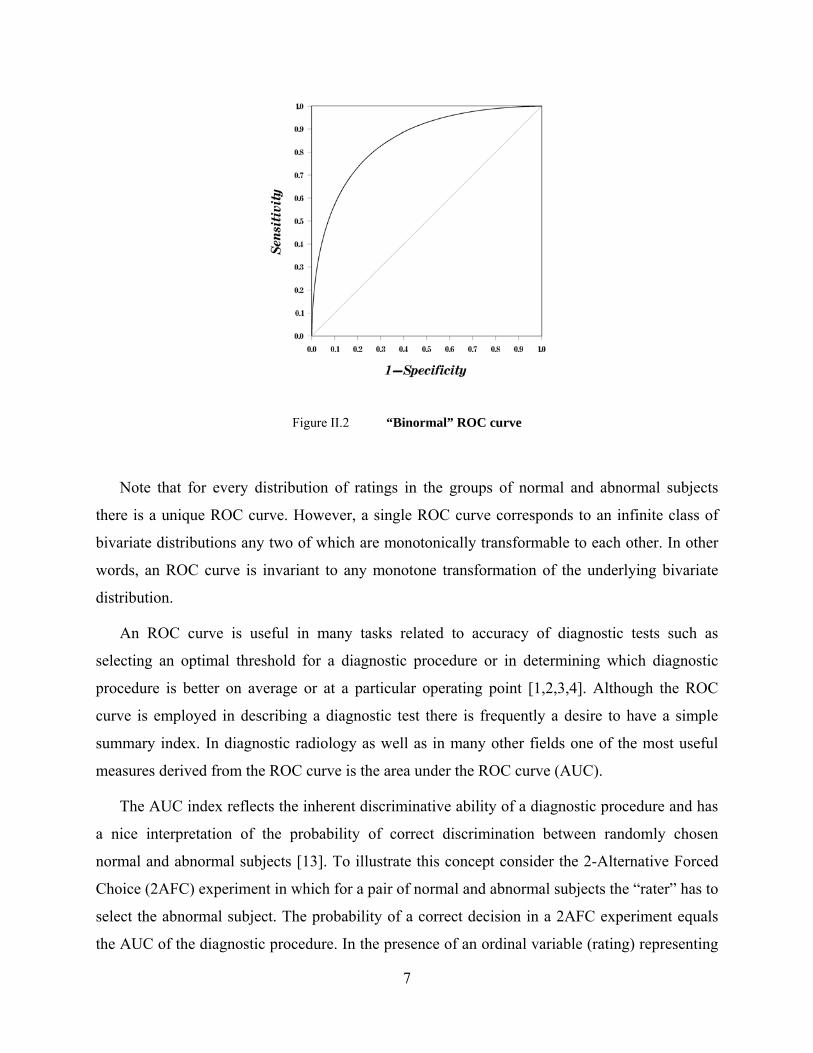
Figure II.2 “Binormal” ROC curve
Note that for every distribution of ratings in the groups of normal and abnormal subjects
there is a unique ROC curve. However, a single ROC curve corresponds to an infinite class of
bivariate distributions any two of which are monotonically transformable to each other. In other
words, an ROC curve is invariant to any monotone transformation of the underlying bivariate
distribution.
An ROC curve is useful in many tasks related to accuracy of diagnostic tests such as
selecting an optimal threshold for a diagnostic procedure or in determining which diagnostic
procedure is better on average or at a particular operating point [1,2,3,4]. Although the ROC
curve is employed in describing a diagnostic test there is frequently a desire to have a simple
sum
f a diagnostic procedure and has
a n
a pair of normal and abnormal subjects the “rater” has to
select the abnormal subject. The probability of a correct decision in a 2AFC experiment equals
the AUC of the diagnostic procedure. In the presence of an ordinal variable (rating) representing
mary index. In diagnostic radiology as well as in many other fields one of the most useful
measures derived from the ROC curve is the area under the ROC curve (AUC).
The AUC index reflects the inherent discriminative ability o
ice interpretation of the probability of correct discrimination between randomly chosen
normal and abnormal subjects [13]. To illustrate this concept consider the 2-Alternative Forced
Choice (2AFC) experiment in which for
7
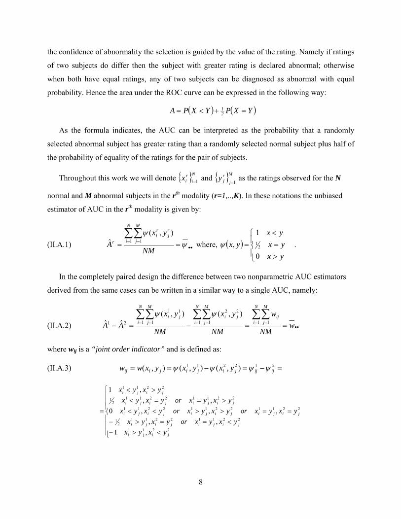
the confidence of abnormality the selection is guided by the value of the rating. Namely if ratings
ubjects do differ then the subject with greater rating is declared abnormal; otherwise
when both have equal ratings, any of two subjects can be diagnosed as abnormal with equal
pro
of two s
bability. Hence the area under the ROC curve can be expressed in the following way:
( ) ( )YXPYXPA 12 =+<=
As the formula indicates, the AUC can be interpreted as the probability that a randomly
abnormal subject has greater rating than a randomly selected normal subject plus half of
the probability of equality of the ratings for the pair of subjects.
ughout this work we will denote
selected
Thro Ni
rix 1= and M
jrjy
1= as the ratings observed for the N
normal and M abnormal subjects in the rth modality (r=1,..,K). In these notations the unbiased
estimator of AUC in the rth modality is given by:
(II.A.1) ••= = ==∑∑
ψψ
NM
yxA
N
i
M
j
rj
ri
r 1 1
),(ˆ where, ( )
⎪⎩
⎪⎨
⎧
>=<
=yxyxyx
yx0
1, 2
1ψ .
In the completely paired design the difference between two nonparametric AUC estimators
derived from the same cases c e w gle AUC, namely:
(II.A.2)
an b ritten in a similar way to a sin
••= == == = ==−=−∑∑∑∑∑∑
wNM
w
NM
yx
NM
yxAA
N
i
M
jij
N
i
M
jji
N
i
M
jji
1 11 1
22
1 1
11
21
),(),(ˆˆ
ψψ
where wij is a “joint order indicator” and is defined as:
(II.A.3) =−=−== 212211 ),(),(),( ijijjijijiij yxyxyxww ψψψψ
⎪⎪⎪
⎩
⎪⎪⎪
⎨
⎧
<>−<==>−
==>><<>==<
><
=
2211
221122112
1
221122112211
221122112
1
2211
,1,,
,,,0,,
,1
jiji
jijijiji
jijijijijiji
jijijiji
jiji
yxyxyxyxoryxyx
yxyxoryxyxoryxyxyxyxoryxyx
yxyx
8

B. METHODS OF ANALYSIS
1.
ximated by a monotone transformation of a binormal distribution. One of the best known
parametric approaches to the analysis of the ROC curves is the maximum likelihood approach
orfman and Alf Jr. [10]. C. Metz et al. have developed computer software
ROCKIT that implements the original [10] and a modified [11] maximum likelihood estimation
h curve [1,6,12,13,14]. The m
abo
sly mentioned, one of the most popul is the Area Under the
ROC Curve (AUC). The nonparametric estimate of the AUC is easy to compute and its
numerical value is equal to the actual area under the estimated ROC curve where empirical
points are connected by straight lines [13]. If
General
Several different methods have been developed for the analysis of ROC curves. The parametric
methods usually model the ROC curves by assuming a particular underlying distribution of
subject ratings (usually assuming that a bivariate distribution of ratings is transformable to a
binormal). The “binormal” ROC curves were shown to be quite robust for a wide class of curves
encountered in practice [9], a property that is in part due to variety of distributions that can be
appro
introduced by D
approaches. The software permits the analysis of two ROC curve in the presence of categorical
or continuous ratings data.
Nonparametric methods utilize empirical ROC points by connecting them with straight lines,
step functions or sometimes by fitting a smoot ain advantage of
nonparametric methods compared to parametric ones is the absence of specific assumptions
ut the shape of the curve or the underlying distribution of ratings. Furthermore, unlike many
parametric procedures, iterative algorithms are not needed for implementation of most
nonparametric methods. A wide family of nonparametric statistics is described by Wieand et al.
[20].
2. AUC index
As previou ar and convenient indices
Niix 1= and M
jjy1= are the ratings observed for the
samples of N nor al and M abnormal subjects then the estimate of the AUC is given in (II.A.1) m
9

The nonparametric AUC estimator as presented in (II.A.1) is a generalized U-statistic and
therefore is approximately normally distributed under quite general assumptions [26]. Hence,
knowing the variance of the estimator is essential for constructing simple asymptotic procedures.
The nonparametric AUC estimator is related to the Mann-Whitney two-sample test statistic
[16,13] and many of the nonparametric approaches to variance derivation are related to the
formula derived by Noether [15] for the Wilcoxon statistic. Using previously introduced
notation, the formula of Noether when applied to the AUC can be written as follows:
(II.B.2.1) 110110111)ˆ( ξξξ MNAVar +
NM NMNM−
+−
= ,
[ ] [ ]AEYXEA jiˆ),( == ψ
[ ] [ YX ×ψψ ] ljAYXEYXYXCov lijiliji ≠−== ,),(),(),(),,( 210 ψψξ
] kiAYXYXYv jkjij ≠−× ,),(),( 2ψψ and [ ] [EYXXCo jki == ),(),,(01 ψψξ
[ ] [ ] 2A 211 ),(),( YXEYXVar jiji −== ψψξ
timator that is based on expressing unknown
expectations using probabilities which can be estimated by proportions. Hanley and McNeil [17]
used the parametric assumption to estimate certain variance elements. The consistent, completely
tric estimators of the covariance matrix for several nonparam tric AUC estimators
were developed by Wieand et al. [18] in 1983 and by DeLong et al. [19] in 1988.
to compute, i.e.:
pute the X- and Y-components:
Bamber [16] proposed an unbiased variance es
nonparame e
The conventional variance estimator proposed by DeLong et al. [19] can also be shown to be
equivalent to the two-sample jackknife estimator of the variance [22]. Because of the structure of
the nonparametric estimator of AUC its variance estimator is easy
a) Com
∑• =M
=jii yx ),(1 ψ ∑
=• =
N
ijij yx
N 1),(1 ψψ
jM 1
ψ ,
b) The components 10ξ and 01ξ are estimated as:
[ ]∑=
••• −−=
N
iiN
s1
2
10 11 ψψ , [ ]∑
=••• −
−=
M
jjM
s1
2
01 11 ψψ
10

c) The consistent estimator of the variance is:
(II.B.3.1) [ ] [ ]
)1()1()ˆ( 1
2
1
2
0110
−−=
∑∑=
•••=
•••ssAV
M
jj
N
ii ψψψψ
−+
−=+
MMNNMN
The estimation approach employed by Wieand et al. [18] when implemented for a single
tors that are equivalent to that proposed by
Bamber [16]. In our notations the unbiased estimator has the following form (both estimators are
AUC produces the biased and unbiased estima
shown in the Appendix C in application to AUC difference):
(II.B.3.2) [ ] [ ] [ ]
)1)(1()1()1()ˆ( 1 1
2
1
2
1
2
−−
+−−−
−
−+
−
−=
∑∑∑∑= =
••••=
•••=
•••
MNNMMMNNAV
N
i
M
jjiij
M
jj
N
ii
W
ψψψψψψψψ
3. Comparing diagnostic modalities
To
agin e
evaluated by all modalities and the ratings obtained in such a way are used for the analysis. The
e subjects can be substantial [27] and should be
accounted for in the analysis.
4. Comparing ROC curves in a paired design
One
. The test they proposed is designed to compare two correlated
ROC curves at every operating point using the specially developed measure denoted as E. The
significance of the observed difference is then evaluated using the permutation space. Namely
the E-index is calculated for every permutation and the p-value is calculated as the proportion of
tim
simplify the discussion we will use the term modality to designate a diagnostic system,
practice or technology. The between subject heterogeneity is recognized as substantial in the
field of diagnostic im g as w ll as in many other fields. Hence, the paired design is often used
to improve the precision of the analysis. In a paired design each subject is independently
correlation between the ratings for the sam
of the nonparametric procedures for comparing ROC curves is a permutation test developed
by Venkatraman and Begg [24]
es when more extreme values than the E-index computed from the observed data are
obtained.
11
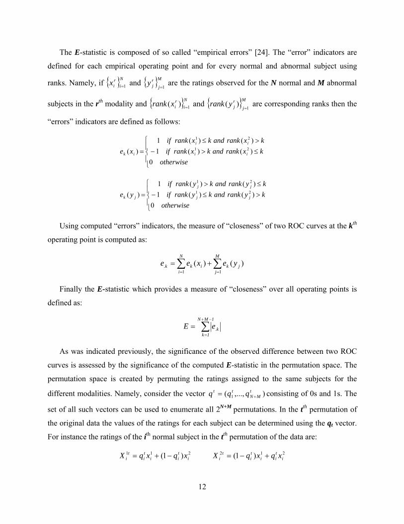
The E-statistic is composed of so called “em errors” [24]. The “error” indicators are
def
pirical
ined for each empirical operating point and for every normal and abnormal subject using
ranks. Namely, if Ni
rix 1= and M
jrjy
1= are the ratings observed for the N normal and M abnormal
subjects in the rth modality and Ni
rixrank 1)( = and Mryrank )( are corresponding ranks then the
“errors” indicators are defined as follows:
⎪
⎪⎨
⎧
≤>−>≤
=otherwise
kxrankandkxrankifkxrankandkxrankif
xe ii
ii
ik )()(1)()(1
)( 21
21
jj 1=
0
⎧
≤≤>
andkykyrankandkyrankif
j
jj
)()()(1
1
21
N
⎩
⎪⎩
⎪⎨ >−=
otherwisekyrankrankifye jjk
0)(1)( 2
Using computed “errors” indicators, the measure of “closeness” of two ROC curves at the kth
operating point is computed as:
∑∑== j
jki
ikk yexee11
. )()(
Finally the E-statistic which provides a measure of “closeness” over all operating points is
defined as:
+=M
∑−+
=1k
1s. The
set of all such vectors can be used to enumerate all 2 permutations. In the tth permutation of
ined using the qt vector.
For instance the ratings of the ith normal subject in the tth permutation of the data are:
=1MN
k.eE
As was indicated previously, the significance of the observed difference between two ROC
curves is assessed by the significance of the computed E-statistic in the permutation space. The
permutation space is created by permuting the ratings assigned to the same subjects for the
different modalities. Namely, consider the vector ),...,( 1t
MNtt qqq += consisting of 0s and
N+M
the original data the values of the ratings for each subject can be determ
211 )1( itii
ti
ti xqxqX −+= 212 )1( i
tii
ti
ti xqxqX +−=
12

Since tiq is either 0 or 1, the vector )X,X( t2
it1
i equals either ),( 21ii xx or ),( 12
ii xx . If all the
permutations are equally likely then the values of the E-statistics computed for all permutations
constitute the “reference” distribution of the E-statistic. The constructed permutations are equally
like
sted to be uniformly broken).
n and
ey found, that compared to the nonparametric “area test” proposed
by DeLong et al. [19], their procedure possesses more power against alternatives of crossing
ROC curves with equal AUC but less power against alternatives of difference in AUCs.
5.
Both parametric and nonparametric methods for comparing correlated AUC indices are
available. The parametric analysis assuming the binormal model was developed by Dorfman and
Alf d further deve Metz et al. [11]. Hanley and McNeil
[17] suggested using the binormal assumption only for estimation of the covariance between two
area estimators.
e eneral class of nonparametric statistics
for comparison of two diagnostic m erage of sensitivities. Earlier,
Wieand, Gail and Hanley developed a nonparametric procedure for comparing diagnostic tests
with paired or unpaired data [18]. DeLong et al. [19] developed a consistent nonparametric
estimator of the covariance matrix for several AUC estimators in a paired design. This method,
whi
ly under the null hypothesis of equality of the ROC curves and the additional assumption of
exchangeability.
To make the procedure appropriate for comparing modalities with different underlying scales
(when ratings are not directly exchangeable even under the null hypothesis), the rank
transformation is suggested. If the transformation is applied then the permutations are conducted
on the rank of the ratings instead of raw ratings (the ties that appeared during the process of
permutation of the ranks are sugge
Venkatrama Begg evaluated operating characteristics of their procedure on simulated
datasets. Due to the computational burden, the p-values were evaluated by sampling from a
permutation distribution. Th
Comparing AUCs with paired data
Jr. [10] and later implemented an loped by
Wi and, Gail, James B and James K [20] described a g
arkers based on a weighted av
ch is described below, is a natural extension to K-samples of the formulas given in Section
II.2.
13

Let and be the ratings assigned by the rth modality (r=1,..,K) to N normal and
M abnormal subjects. Then the vector of the AUC estimators can be computed as a simple
average of the order indicators, i.e.:
Ni
rix 1= M
jrjy
1=
( )KKAA ••••= ψψ ,...,)ˆ,...,ˆ(11
The covariance matrix for a vector the estimators )A,...,A( K1 can be computed as follows:
a) Compute the X and Y components of the rth modality,
∑=
• =M
j
rj
ri
ri yx
M 1
),(1 ψψ , ∑=
• =N
i
rj
ri
r
j yxN 1
),(1 ψψ
K1s,r
s,r1010 sS == and K
1s,rs,r
0101 sS ==b) Compute the matrices , where
[ ] [ ]∑=
•••••• −×−−
=N
i
ss
i
rr
isr
Ns
1
,10 1
1 ψψψψ , [ ] [ ]∑=
•••••• −×−−
=M
j
ss
j
rr
jsr
Ms
1
,01 1
1 ψψψψ
c) A consistent estimator of the covariance matrix is:
MS
NS
AAvoC K 01101 )ˆ,...,ˆ(ˆ += the (r,s)th element of which is
[ ] [ ] [ ] [ ])1()1(
)ˆ,ˆ(ˆ 11
−
−×−+
−
−×−=
∑∑=
••••••=
••••••
MMNNAAvoC
M
j
ssj
rrj
N
i
ssi
rri
sr
ψψψψψψψψ
Using our notation, the unbiased estimator proposed by Wieand et al. [18] takes the
following form:
[ ] [ ] [ ] [ ]−
−
−×−+
−
−×−=
∑∑=
••••••=
••••••
)1()1()ˆ,ˆ(ˆ 11
MMNNAAvoC
M
j
ssj
rrj
N
i
ssi
rri
sr
ψψψψψψψψ
[ ] [ ])1)(1(
1 1
−−
+−−×+−−−∑∑= =
••••••••
MNNM
N
i
M
j
ssj
si
sij
rrj
ri
rij ψψψψψψψψ
Note that in a completely paired design, the variance of the difference between the
nonparametric estimators of AUC can be found using formulas (II.B.3.1-2) but employing the
difference of the order indicators (II.A.3) instead of the original indicators
(Appendix C).
21ijijijw ψψ −=
14
III. PROPERTIES OF THE CONVENTIONAL NONPARAMETRIC TEST
The conventional nonparametric test for comparing correlated AUCs proposed by DeLong et al.
[19] uses a consistent variance estimator and relies on asymptotic normality of the AUC
estimator. Although it is generally recognized that convergence to the asymptotic properties
depends on the underlying parameters, and several Monte Carlo studies include the conventional
procedure in their investigation [38,39,40], there have not been extensive simulations
characterizing the effects of relevant parameters on the small-sample properties of the this
procedure.
We study the behavior of the type I error and the statistical power of the conventional
nonparametric test for comparing two AUCs over a wide range of relevant parameters and
against various alternatives. These investigations provide useful information on the effect of
selected underlying parameters on small-sample statistical inferences. Part of the results of this
investigation was presented at the MIPS conference [31].
A. GENERAL SIMULATION DESCRIPTION
To model the ratings assigned to a sample of subjects by two diagnostic modalities we simulate
the data from two correlated bivariate (normal and abnormal subjects’) distributions. For our
simulations we use the “binormal” ROC model because of its simplicity and robustness [9] Thus,
within the rth modality, subjects’ ratings are generated from binormal distributions namely,
, for the ratings of the normal subjects and ),(~...
rY
rY
diiNY σµ , for the ratings of
the abnormal subjects. Furthermore, to model a paired data structure a correlation of magnitude,
ρ, is induced for the ratings of the same sub
),(~...
rX
rX
diiri NX σµ r
j
ject in different modalities
15

( ρ== ),(),( 2121 YYCovXXCov ). Note that the use of the binormal distribution to model
subjects’ ratings provides considerable flexibility since the ROC curve and ROC techniques that
we consider are invariant with respect to order-preserving transformation of the data.
The binormal ROC curve corresponding to the distribution of ratings within the rth modality
can be parameterized using the following quantities:
( )rrr - the Area Under the ROC Curve, and YXPA <=
rY
rX
rbσσ
= - the shape-parameter
By varying the parameters of the distributions of the ratings we model various patterns of the
correlation between the ratings of the same subjects (ρ), average of two AUCs (A), difference
between two areas (∆) and shapes of the ROC curve (b). The scenario of non-crossing ROC
curves is modeled by setting b=1 for both modalities while crossing ROC curves were simulated
by setting b<1 (corresponds to a greater variability among ratings of abnormal subjects) for one
of the modalities. We also considered different values of the total number of normal and
abnormal subjects (T=N+M) and of the proportion of subjects with an abnormality
(p=M/(N+M)). For each considered scenario 10,000 datasets were simulated.
B. SIMULATION STUDY
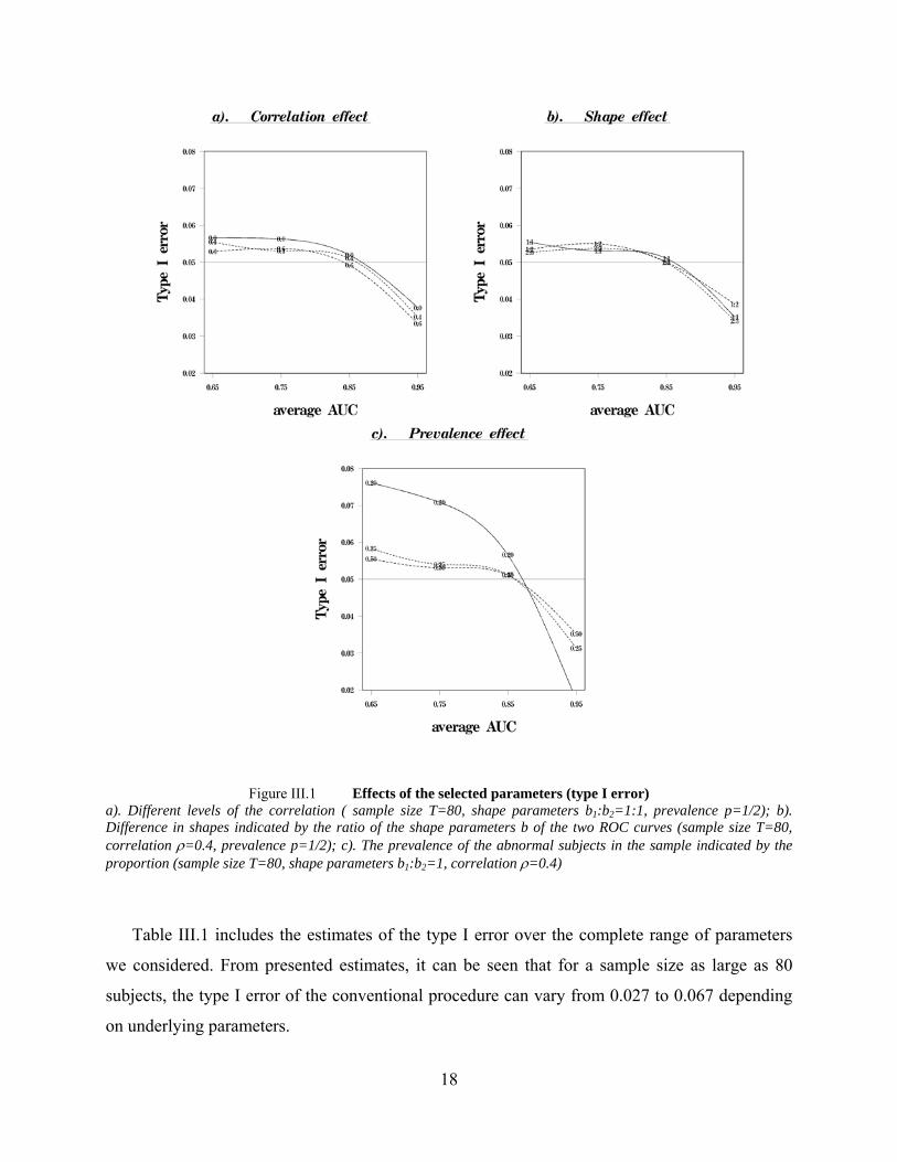
The effects of the selected parameters on the type I error of the conventional test for comparing
correlated AUCs are summarized in Figure III.1 and Table III.1. Figure III.2 and Table III.2
depict the effect of selected parameters on the statistical power of the procedure. Each figure is
only able to summarize the trend in the rejection rate for two parameters and therefore the other
parameters are kept fixed at what is considered reasonable values. Specifically, when the value
of a parameter is not specified on the graph it is set to one of the following: sample size (T) of
80, an average AUC (A) of 0.85, a correlation between ratings (ρ) of 0.4, a shape parameter (b)
of 1 in both modalities and “prevalence” of the abnormal subjects (p) of ½.
16

All graphs in Figure III.1 demonstrate the substantial effect of the underlying AUC on the
false rejection rate of the conventional test. Namely, the type I error decreases with increasing
average AUC (A) shifting from being slightly elevated above the nominal level to being
sub
tistical test
(Fi
ed sample is depicted on Figure
III.1.c. It can be noted that imbalance of the selected sample affects the behavior of the type I
error by strengthening its dependence on the underlying AUC.
stantially lower. Although other parameters can slightly change the rate of the relationship the
general decreasing pattern remains the same.
From the Figure III.1.a, one can note a moderate but distinct effect of the correlation
(adjusted for the effect of AUC). The graph suggests that increasing correlation may decrease the
type I error independently from the AUC. The difference in shapes of the ROC curves that have
equal AUCs does not greatly affect the false rejection rate (type I error) of the sta
gure III.1.b). However the complete results of our investigation of the type I error (Table
III.1) suggests a small increase of the false rejection rate when the ROC curves cross.
The effect of prevalence of abnormal subjects in a select
17
18
Figure III.1 Effects of the selected parameters (type I error) a). Different levels of the correlation ( sample size T=80, shape parameters b1:b2=1:1, prevalence p=1/Difference in shapes indicated by the ratio of the shape parameters b of the two ROC curves (sample size T=8correlation ρ=0.4, prevalence p=1/2); c). The prevalence of the abnormal subjects in the sample indicatedproportion (sample size T=80, shape parameters b1:b2=1, correlation ρ=0.4)
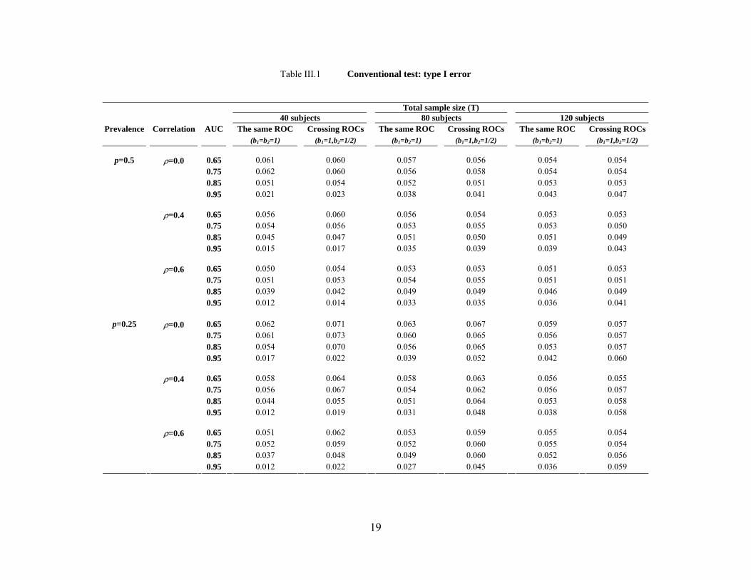
Table III.1 includes the estimates of the type I error over the complete range of param
we considered. From presented estimates, it can be seen that for a sample size as larg
subjects, the type I error of the conventional procedure can vary from 0.027 to 0.067 depending
on underlying parameters.
2); b). 0,
by the
eters
e as 80
19
Table III.1 Conventional test: type I error
Total sample size (T) 40 subjects 80 subjects 120 subjects
Prevalence Correlation AUC The same ROC Crossing ROCs The same ROC Crossing ROCs The same ROC Crossing ROCs (b1=b2=1)
(b1=1,b2=1/2) (b1=b2=1) (b1=1,b2=1/2) (b1=b2=1)
(b1=1,b2=1/2)
ρ=0.0 0.65
0.061 0.060 0.057 0.056 0.054 0.054 0.75 0.062 0.060 0.056 0.058 0.054 0.054 0.85 0.051 0.054 0.052 0.051 0.053 0.053
0.95
0.021 0.023 0.038 0.041 0.043 0.047
ρ=0.4 0.65 0.056 0.060 0.056 0.054 0.053 0.053 0.75 0.054 0.056 0.053 0.055 0.053 0.050 0.85 0.045 0.047 0.051 0.050 0.051 0.049
0.95
0.015 0.017 0.035 0.039 0.039 0.043
ρ=0.6 0.65 0.050 0.054 0.053 0.053 0.051 0.053 0.75 0.051 0.053 0.054 0.055 0.051 0.051 0.85 0.039 0.042 0.049 0.049 0.046 0.049
p=0.5
0.95
0.012 0.014 0.033 0.035 0.036 0.041
ρ=0.0 0.65 0.062 0.071 0.063 0.067 0.059 0.057 0.75 0.061 0.073 0.060 0.065 0.056 0.057 0.85 0.054 0.070 0.056 0.065 0.053 0.057
0.95
0.017 0.022 0.039 0.052 0.042 0.060
ρ=0.4 0.65 0.058 0.064 0.058 0.063 0.056 0.055 0.75 0.056 0.067 0.054 0.062 0.056 0.057 0.85 0.044 0.055 0.051 0.064 0.053 0.058
0.95
0.012 0.019 0.031 0.048 0.038 0.058
ρ=0.6 0.65 0.051 0.062 0.053 0.059 0.055 0.054 0.75 0.052 0.059 0.052 0.060 0.055 0.054
0.85 0.037 0.048 0.049 0.060 0.052 0.056
p=0.25
0.95 0.012 0.022 0.027 0.045 0.036 0.059

The effects of the selected parameters on the statistical power of the conventional test are
summarized in Figure III.2 and Table III.2. The relative order of the effects of the parameters
remains similar to that observed for the type I error with the average AUC having the largest
effect and the difference in shapes of the ROC curves having the smallest effect. However the
direction of the relationships does differ. Namely increasing the average AUC or correlation tend
increase the statistical power of the conventional test for large AUC differences in contrast to
decreasing its type I error (Figure III.2.a,d). Increasing balance between the numbers of subjects
in the selected sample not only improves the rate of false rejection (type I error) of the statistical
test making it closer to the nominal level but also tend to increase the rate of its true rejections
(power) for large AUC differences.
20
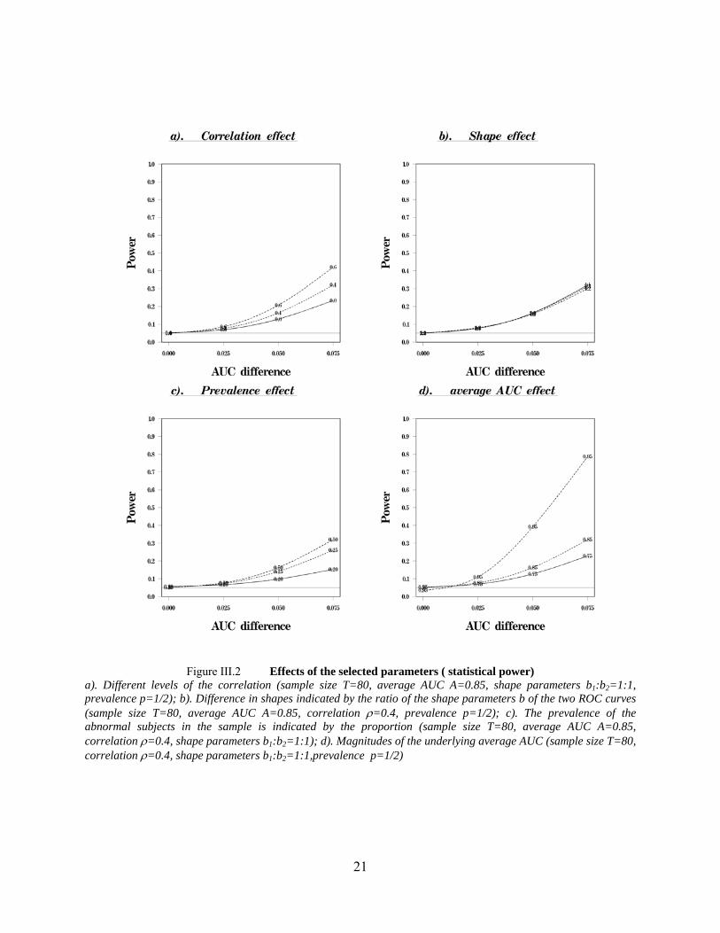
selected parameters ( statistical power) Figure III.2 Effects of thea). Different levels of the correlation (sample size T=80, average AUC A=0.85, shape parameters b1:b2=1:1, prevalence p=1/2); b). Difference in shapes indicated by the ratio of the shape parameters b of the two ROC curves (sample size T=80, average AUC A=0.85, correlation ρ=0.4, prevalence p=1/2); c). The prevalence of the abnormal subjects in the sample is indicated by the proportion (sample size T=80, average AUC A=0.85, correlation ρ=0.4, shape parameters b1:b2=1:1); d). Magnitudes of the underlying average AUC (sample size T=80, correlation ρ=0.4, shape parameters b1:b2=1:1,prevalence p=1/2)
21
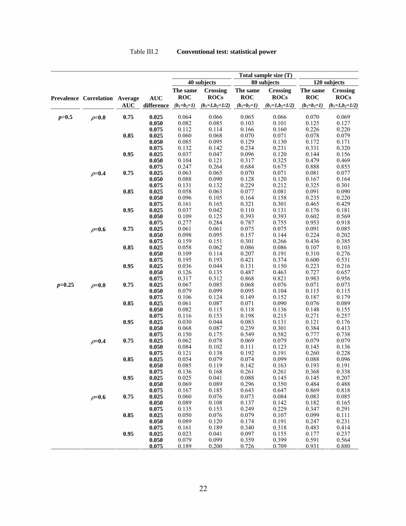
Table III.2 Conventional test: statistical power
Total sample size (T) 40 subjects 80 subjects 120 subjects
Prevalence Correlation Average AUC The same
ROC Crossing
ROCs The same
ROC Crossing
ROCs The same ROC
Crossing ROCs
AUC difference (b1=b2=1) (b1=1,b2=1/2) (b1=b2=1) (b1=1,b2=1/2) (b1=b2=1) (b1=1,b2=1/2)
0.75 0.025 0.064 0.066 0.065 0.066 0.070 0.069 0.050 0.082 0.085 0.103 0.101 0.125 0.127 0.075 0.112 0.114 0.166 0.160 0.226 0.220 0.85 0.025 0.060 0.068 0.070 0.071 0.078 0.079 0.050 0.085 0.095 0.129 0.130 0.172 0.171 0.075 0.132 0.142 0.234 0.231 0.331 0.320 0.95 0.025 0.037 0.047 0.096 0.120 0.144 0.156 0.050 0.104 0.121 0.317 0.325 0.479 0.469
ρ=0.0
0.075 0.247 0.264 0.684 0.675 0.888 0.855 0.75 0.025 0.063 0.065 0.070 0.071 0.081 0.077 0.050 0.088 0.090 0.128 0.120 0.167 0.164 0.075 0.131 0.132 0.229 0.212 0.325 0.301 0.85 0.025 0.058 0.063 0.077 0.081 0.091 0.090 0.050 0.096 0.105 0.164 0.158 0.235 0.220 0.075 0.161 0.165 0.321 0.301 0.465 0.429 0.95 0.025 0.037 0.042 0.110 0.131 0.176 0.181 0.050 0.109 0.125 0.393 0.393 0.602 0.569
ρ=0.4
0.075 0.277 0.284 0.787 0.755 0.953 0.918 0.75 0.025 0.061 0.061 0.075 0.075 0.091 0.085 0.050 0.098 0.095 0.157 0.144 0.224 0.202 0.075 0.159 0.151 0.301 0.266 0.436 0.385 0.85 0.025 0.058 0.062 0.086 0.086 0.107 0.103 0.050 0.109 0.114 0.207 0.191 0.310 0.276 0.075 0.195 0.193 0.421 0.374 0.600 0.531 0.95 0.025 0.036 0.044 0.131 0.150 0.223 0.216 0.050 0.126 0.135 0.487 0.463 0.727 0.657
p=0.5
ρ=0.6
0.075 0.317 0.312 0.868 0.821 0.983 0.956 0.75 0.025 0.067 0.085 0.068 0.076 0.071 0.073 0.050 0.079 0.099 0.095 0.104 0.115 0.115 0.075 0.106 0.124 0.149 0.152 0.187 0.179 0.85 0.025 0.061 0.087 0.071 0.090 0.076 0.089 0.050 0.082 0.115 0.118 0.136 0.148 0.155 0.075 0.116 0.153 0.198 0.215 0.271 0.257 0.95 0.025 0.030 0.044 0.083 0.131 0.121 0.176 0.050 0.068 0.087 0.239 0.301 0.384 0.413
ρ=0.0
0.075 0.150 0.175 0.549 0.582 0.777 0.738 0.75 0.025 0.062 0.078 0.069 0.079 0.079 0.079 0.050 0.084 0.102 0.111 0.123 0.145 0.136 0.075 0.121 0.138 0.192 0.191 0.260 0.228 0.85 0.025 0.054 0.079 0.074 0.099 0.088 0.096 0.050 0.085 0.119 0.142 0.163 0.193 0.191 0.075 0.136 0.168 0.261 0.261 0.368 0.338 0.95 0.025 0.025 0.041 0.088 0.145 0.145 0.207 0.050 0.069 0.089 0.296 0.350 0.484 0.488
ρ=0.4
0.075 0.167 0.185 0.643 0.647 0.869 0.818 0.75 0.025 0.060 0.076 0.073 0.084 0.083 0.085 0.050 0.089 0.108 0.137 0.142 0.182 0.165 0.075 0.135 0.153 0.249 0.229 0.347 0.291 0.85 0.025 0.050 0.076 0.079 0.107 0.099 0.111 0.050 0.089 0.120 0.174 0.191 0.247 0.231 0.075 0.161 0.189 0.340 0.318 0.483 0.414 0.95 0.025 0.023 0.041 0.097 0.155 0.177 0.237 0.050 0.079 0.099 0.359 0.399 0.591 0.564
p=0.25
ρ=0.6
0.075 0.189 0.200 0.726 0.709 0.931 0.880
22
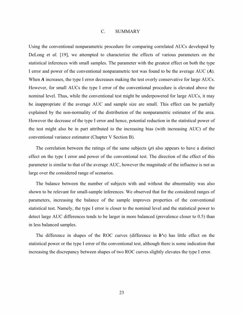
C. SUMMARY
Using the conventional nonparametric procedure for comparing correlated AUCs developed by
DeLong et al. [19], we attempted to characterize the effects of various parameters on the
statistical inferences with small samples. The parameter with the greatest effect on both the type
I error and power of the conventional nonparametric test was found to be the average AUC (A).
When A increases, the type I error decreases making the test overly conservative for large AUCs.
However, for small AUCs the type I error of the conventional procedure is elevated above the
nominal level. Thus, while the conventional test might be underpowered for large AUCs, it may
be inappropriate if the average AUC and sample size are small. This effect can be partially
explained by the non-normality of the distribution of the nonparametric estimator of the area.
However the decrease of the type I error and hence, potential reduction in the statistical power of
the test might also be in part attributed to the increasing bias (with increasing AUC) of the
conventional variance estimator (Chapter V Section B).
The correlation between the ratings of the same subjects (ρ) also appears to have a distinct
effect on the type I error and power of the conventional test. The direction of the effect of this
parameter is similar to that of the average AUC, however the magnitude of the influence is not as
large over the considered range of scenarios.
The balance between the number of subjects with and without the abnormality was also
shown to be relevant for small-sample inferences. We observed that for the considered ranges of
parameters, increasing the balance of the sample improves properties of the conventional
statistical test. Namely, the type I error is closer to the nominal level and the statistical power to
detect large AUC differences tends to be larger in more balanced (prevalence closer to 0.5) than
in less balanced samples.
The difference in shapes of the ROC curves (difference in b’s) has little effect on the
statistical power or the type I error of the conventional test, although there is some indication that
increasing the discrepancy between shapes of two ROC curves slightly elevates the type I error.
23
IV. PERMUTATION TEST
In this chapter we develop the permutation test for detecting differences between two AUCs in a
paired design setting. Such a permutation procedure not only provides an exact (suitable for
small samples) and powerful test for detecting differences in overall performances but also
permits developing a precise and easy-to-apply approximation. The availability of a simple and
precise approximation to the permutation test is a desirable property since, with increasing
sample size the exact permutation tests quickly become very demanding computationally. We
also conduct simulations to investigate properties of the new procedure. The material in this
chapter is accepted for publication in Statistics in Medicine [32].
A. EXACT PERMUTATION TEST
In order to compare the AUCs of the two correlated ROC Curves we propose a permutation test
in which the values of the estimator of the AUC difference computed from all possible
permutations constitute the distribution of the estimator under the null hypothesis. If the two
modalities had the same underlying scale of ratings we could justify directly permuting the actual
ratings for each subject. However, since the ROC curves are invariant with respect to monotone
transformations of the data, without loss of generality we can permute the rank of the ratings (or
appropriate monotonic transformation of the ratings) as if they were actual ratings on the same
underlying scale. Hence the use of the transformed ratings allows us to compare the modalities
with different underlying scales as well. We will refer to monotonically transformed ratings or
ranks of the ratings as rank-ratings.
The proposed test is conducted by permuting the subject specific rank-ratings between the
two modalities within the structure of given pairs. The 2N+M permutations are created by
24

exchanging the rank-rating observed for each subject for the two modalities, and permutations
for different subjects are done independently of each other. Thus if for the ith normal subject (Xi)
and jth abnormal subject (Yj) the rank-ratings observed in first and second modality are
respectively then all possible permutations that can be performed with those two
subjects are as follows:
2j
1j
2i
1i yandy,x,x
(IV.A.1)
changedexs'Y,changedexs'X)y,x()y,x(
changedexs'Y,changedexnots'X)y,x()y,x(
changedexnots'Y,changedexs'X)y,x()y,x(
changedexnots'Y,changedexnots'X)y,x()y,x(
2j
1i
1j
2i
2j
2i
1j
1i
−
−−
modIImod
−
metric with respect to its arguments
(separately for the normal and abnormal subjects) [24]. The exchangeability assumption is a
stricter assumption than the equality of the ROC curves. We consider our procedure to have as a
null hypothesis equality of ROC curves under the assumption of exchangeability. The
utations α/2 and 1-α/2
percentile values. The two-sided p-value can be defined as:
I
1j
1i
2j
2i
1j
2i
2j
1i
−−
−−
where the pairs in the first column are assumed to be observed for the first modality and the pairs
in the second column are assumed to be observed for the second modality.
To justify equal probability of all permutations under the null hypothesis, we assume the
exchangeability of the subject specific rank-ratings between the two modalities. Exchangeability
means that the joint distribution of the rank-ratings is sym
distribution of the differences in the estimated Areas under the ROC Curves over all
perm is readily obtained and the rejection region can be selected based on
MNMN
tt
tAAAA
AAAAPp ++Ω =⎭
⎬⎫
⎩⎨⎧
−≥−=⎟⎟
⎠
⎞⎜⎜⎝
⎛−≥−= 2,...,1
2
ˆˆˆˆ#ˆˆˆˆ
20
10
21
20
10
21
where 2N+M is the total number of all possible permutations, 20
10 AA − - is the observed AUC
difference and 2t
1t AA − is the AUC difference computed from the tth permutation.
25

Properties of the difference between two nonparametric AUC estimators allow for the
construction of a simple asymptotic procedure. As a member of the class of U-statistics the
par
estimator of the AUC is unbiased,
the expectation of the AUC difference is 0 when the two AUCs are equal and this fact is also
illustrated in the permutation space Ω under the stricter assumption of exchangeability (see
Ap
tion space as sh
Hence, under the assumption of asymptotic normality of the U-statistic and the additional
k-ratings:
ametric estimator of the AUC difference is known to be asymptotically normally distributed
under quite general conditions [26]. Since the nonparametric
pendix A). The exchangeability assumption also allows a simple calculation of the exact
variance of the AUC difference in the permuta own in Appendix A.
assumption of exchangeability of within subject ran
( ) )1,0(ˆˆ
ˆˆ21
21
NAAVar
AA d⎯→⎯−
−
Ω
.
Thus, a test of the hypothesis of equality of ROC curves that is sensitive to the differences in
AUCs can be conducted using the statistic ( )21
20
10
ˆˆ
ˆˆ
AAVar
AA
−
−
Ω
, where the exact variance in the
denominator is obtained as shown in Appendix A.
B. SIMULATION STUDY
c both
con
We performed extensive computer simulations to investigate the type I error and the statistical
power of the asymptotic procedure for different underlying AUCs, correlations between subject
ratings across modalities and different sample sizes. In our simulations we assume equal
orrelation across modalities for the ratings of normal and abnormal subjects rated on
tinuous and discrete scales and consider scenarios with non-crossing as well as crossing ROC
curves.
The general protocol of simulations follows the approach described in Chapter II, Section A.
In addition to simulations of continuous datasets, we also investigated the rejection rate of the
proposed procedure in the discrete case. The discrete ratings were simulated by grouping the
26

27
ed here are limited to small sample sizes. However, even with these small samples there
ent between the exact and approximate test. The simulations in Table IV.1 show
that even for six normal and six abnormal subjects the asymptotic test is adequate. (In general we
found that it is feasible to conduct the exact test with the sample size as large as fifteen normal
and fifteen abnormal subjects without using a large amount of computer time.) Thus, for the
larger sample sizes as presented in subsequent tables we simulate only the operating
characteristics of the asymptotic test since the results for the exact test should be essentially the
same.
binormal data into 5 categories. The parameters of each pair of binormal distributions (A, b and
ρ) were selected to produce predetermined parameters in the resultant discrete distributions.
Table IV.1 compares the type I error and the statistical power of the exact permutation test to
its normal approximation. Note that the rejection rate formally corresponds to the Type I error of
the proposed procedure in cases of equal ROC curves (non-crossing ROC curves with 0 AUC
difference) and to the power in all other cases considered. Due to the relatively large
computational time required for the implementation of the exact procedure the comparisons
present
is a good agreem

28
Table IV.1 Exact procedure vs. its approximation: rejection rate
Non-crossing ROC curves (b1=b2=1) Crossing ROC curves (b1=1,b2=1/2) ρ=0.0 ρ=0.4 ρ=0.6 ρ=0.0 ρ=0.4 ρ=0.6 Average
AUC
AUC difference
Asymptotic Exact Asymptotic Exact Asymptotic Exact Asymptotic Exact Asymptotic Exact Asymptotic Exact
0.70
0.027
0.00 0.045 0.047 0.044 0.048 0.045 0.050 0.047 0.051 0.049 0.054 0.047 0.0530.05 0.048 0.051 0.051 0.055 0.051 0.057 0.051 0.055 0.055 0.060 0.056 0.0620.10 0.064 0.066 0.069 0.076 0.080 0.086 0.068 0.069 0.074 0.081 0.081 0.0920.15 0.089 0.093 0.108 0.114 0.133 0.143 0.093 0.098 0.110 0.121 0.130 0.1440.20 0.123 0.128 0.161 0.169 0.205 0.222 0.130 0.133 0.165 0.176 0.202 0.220
0.75
0.00 0.037 0.040 0.039 0.044 0.039 0.043 0.039 0.043 0.039 0.046 0.039 0.0460.05 0.046 0.047 0.046 0.050 0.046 0.051 0.046 0.048 0.045 0.051 0.048 0.0560.10 0.060 0.063 0.065 0.070 0.074 0.082 0.063 0.066 0.069 0.077 0.076 0.0850.15 0.084 0.087 0.103 0.111 0.125 0.137 0.090 0.095 0.107 0.117 0.128 0.1430.20 0.121 0.127 0.160 0.172 0.202 0.224 0.130 0.139 0.165 0.181 0.201 0.228
0.80
0.00 0.031 0.033 0.030 0.035 0.031 0.034 0.033 0.037 0.032 0.039 0.033 0.0410.05 0.035 0.037 0.037 0.042 0.038 0.045 0.038 0.041 0.038 0.046 0.043 0.0490.10 0.051 0.054 0.057 0.065 0.066 0.077 0.055 0.060 0.061 0.072 0.070 0.0810.15 0.076 0.081 0.097 0.109 0.124 0.140 0.083 0.088 0.101 0.114 0.123 0.1420.20 0.116 0.124 0.159 0.178 0.208 0.233 0.122 0.130 0.164 0.184 0.204 0.236
0.85
0.00 0.020 0.023 0.024 0.022 0.025 0.022 0.027 0.023 0.029 0.025 0.0290.05 0.025 0.027 0.030 0.034 0.031 0.034 0.027 0.029 0.031 0.037 0.035 0.0390.10 0.039 0.041 0.051 0.057 0.063 0.070 0.042 0.045 0.054 0.062 0.063 0.0740.15 0.064 0.068 0.091 0.102 0.117 0.135 0.069 0.074 0.093 0.107 0.117 0.1410.20 0.109 0.116 0.155 0.176 0.203 0.237 0.113 0.123 0.160 0.182 0.203 0.238
0.90
0.00 0.010 0.012 0.012 0.013 0.014 0.015 0.010 0.012 0.015 0.017 0.016 0.0180.05 0.012 0.015 0.020 0.021 0.023 0.024 0.015 0.017 0.021 0.023 0.026 0.0280.10 0.027 0.030 0.044 0.047 0.059 0.063 0.029 0.033 0.047 0.052 0.061 0.0670.15 0.055 0.060 0.087 0.098 0.118 0.137 0.057 0.062 0.092 0.102 0.121 0.138
0.95 0.00 0.002 0.002 0.004 0.003 0.007 0.005 0.003 0.002 0.004 0.004 0.007 0.005 0.05 0.005 0.005 0.013 0.011 0.017 0.015 0.005 0.005 0.014 0.012 0.018 0.016
Simulated samples consist of 6 normal and 6 abnormal subjects

29
We compared the rejection rate of the proposed asymptotic test to that of the conventional
nonparametric procedure developed by DeLong et al. [19]. The estimates are presented in Table
IV.2 for continuous data and Table IV.3 for discrete data. Note that in these tables the rejection
rate provides the estimates of the type I error of the conventional procedure for all combinations
of parameters we considered. However, since the null hypothesis of the proposed procedure is
formally the equality of ROC curves subject to exchangeability, in situations of crossing ROC
curves the rejection rate is the statistical power. For moderate sample sizes and for the scenario
where non-crossing ROC curves have equal and large AUC that are at least moderately
correlated between modalities, the proposed permutation test demonstrates a type I error that is
less conservative than the conventional test. This effect is especially evident with smaller sample
sizes.
For equal AUCs arising from crossing ROC curves the rejection rate of the permutation test
(power) is very close to that of the conventional nonparametric area test (type I error). The
practical relevance of this finding is that the proposed procedure should not be used to detect
crossing ROC curves with the same AUCs. However, the closeness of the rejection rate to the
nominal significance level suggests that even though the proposed procedure is formally a test
for equality of ROC curves it provides an approximate test of equality of AUCs. As such, it is
useful to compare the power of the proposed procedure to that of the conventional method of
DeLong et al. [19].
For non-crossing ROC curves with a correlation ρ≥0.4 and an average AUC A≥0.80 the
power of the proposed test is greater than that of the conventional procedure (Table IV.4). This
power increase is expected because the proposed test is less conservative in this range of
parameters. For lower correlations and smaller average AUCs, DeLong et al.’s procedure has
slightly greater power. However, this is a region where the type I error of the conventional test is
slightly elevated. With increasing sample size the operating characteristics of the two procedures
approach each other. For crossing ROC curves (Table IV.5), the pattern is similar. Specifically,
for higher correlations and higher average areas the rejection rate for the proposed test is higher.
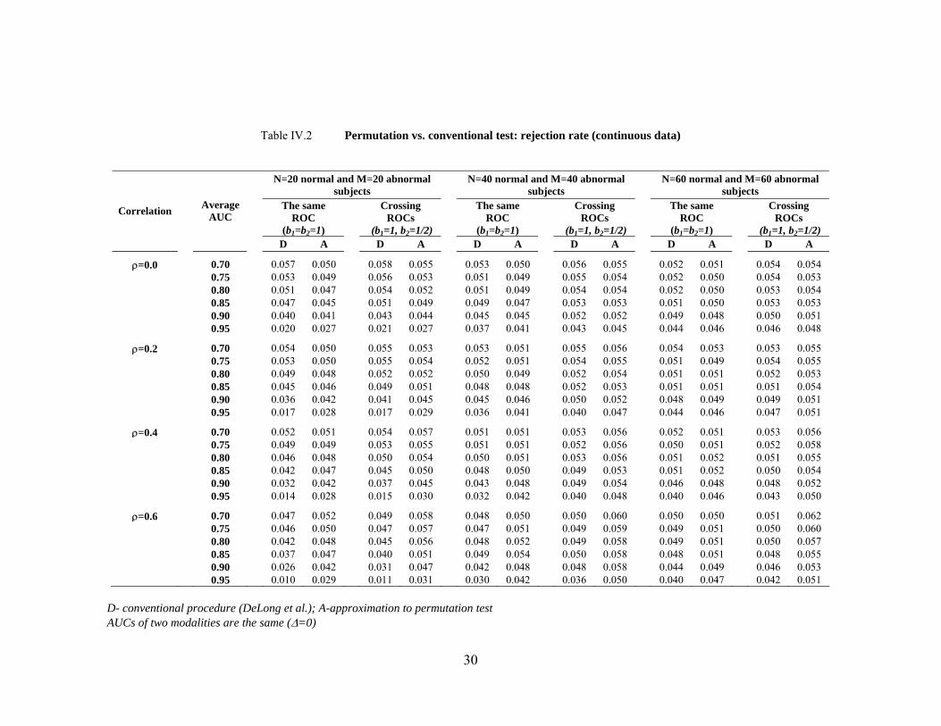
Table IV.2 Permutation vs. conventional test: rejection rate (continuous data)
N=20 normal and M=20 abnormal subjects N=40 normal and M=40 abnormal
subjects N=60 normal and M=60 abnormal subjects
The same
ROC (b1=b2=1)
Crossing
ROCs (b1=1, b2=1/2)
The same
ROC (b1=b2=1)
Crossing
ROCs (b1=1, b2=1/2)
The same
ROC (b1=b2=1)
Crossing
ROCs (b1=1, b2=1/2)
Correlation
Average AUC
D A D A D A D A D A D A
ρ=0.0
0.70 0.057 0.050 0.058 0.055 0.053 0.050 0.056 0.055 0.052 0.051 0.054 0.0540.75 0.053 0.049 0.056 0.053 0.051 0.049 0.055 0.054 0.052 0.050 0.054 0.053
0.80 0.051 0.047 0.054 0.052 0.051 0.049 0.054 0.054 0.052 0.050 0.053 0.0540.85 0.047 0.045 0.051 0.049 0.049 0.047 0.053 0.053 0.051 0.050 0.053 0.0530.90 0.040 0.041 0.043 0.044 0.045 0.045 0.052 0.052 0.049 0.048 0.050 0.0510.95 0.020 0.027 0.021 0.027 0.037 0.041 0.043 0.045 0.044 0.046 0.046 0.048
ρ=0.2
0.70 0.054 0.050 0.055 0.053 0.053 0.051 0.055 0.056 0.054 0.053 0.053 0.0550.75 0.053 0.050 0.055 0.054 0.052 0.051 0.054 0.055 0.051 0.049 0.054 0.055
0.80 0.049 0.048 0.052 0.052 0.050 0.049 0.052 0.054 0.051 0.051 0.052 0.0530.85 0.045 0.046 0.049 0.051 0.048 0.048 0.052 0.053 0.051 0.051 0.051 0.0540.90 0.036 0.042 0.041 0.045 0.045 0.046 0.050 0.052 0.048 0.049 0.049 0.0510.95 0.017 0.028 0.017 0.029 0.036 0.041 0.040 0.047 0.044 0.046 0.047 0.051
ρ=0.4
0.70 0.052 0.051 0.054 0.057 0.051 0.051 0.053 0.056 0.052 0.051 0.053 0.0560.75 0.049 0.049 0.053 0.055 0.051 0.051 0.052 0.056 0.050 0.051 0.052 0.058
0.80 0.046 0.048 0.050 0.054 0.050 0.051 0.053 0.056 0.051 0.052 0.051 0.0550.85 0.042 0.047 0.045 0.050 0.048 0.050 0.049 0.053 0.051 0.052 0.050 0.0540.90 0.032 0.042 0.037 0.045 0.043 0.048 0.049 0.054 0.046 0.048 0.048 0.0520.95 0.014 0.028 0.015 0.030 0.032 0.042 0.040 0.048 0.040 0.046 0.043 0.050
ρ=0.6
0.70 0.047 0.052 0.049 0.058 0.048 0.050 0.050 0.060 0.050 0.050 0.051 0.0620.75 0.046 0.050 0.047 0.057 0.047 0.051 0.049 0.059 0.049 0.051 0.050 0.060
0.80 0.042 0.048 0.045 0.056 0.048 0.052 0.049 0.058 0.049 0.051 0.050 0.0570.85 0.037 0.047 0.040 0.051 0.049 0.054 0.050 0.058 0.048 0.051 0.048 0.0550.90 0.026 0.042 0.031 0.047 0.042 0.048 0.048 0.058 0.044 0.049 0.046 0.053
0.95 0.010 0.029 0.011 0.031 0.030 0.042 0.036 0.050 0.040 0.047 0.042 0.051
D- conventional procedure (DeLong et al.); A-approximation to permutation test AUCs of two modalities are the same (∆=0)
30

Table IV.3 Permutation vs. conventional test: rejection rate (discrete data)
N=20 normal and M=20 abnormal subjects N=40 normal and M=40 abnormal
subjects N=60 normal and M=60 abnormal subjects
The same ROC (b1=b2=1)
Crossing ROCs (b1=1,b2=1/2)
The same ROC (b1=b2=1)
Crossing ROCs (b1=1,b2=1/2)
The same ROC (b1=b2=1)
Crossing ROCs (b1=1,b2=1/2)
Correlation
AUC
D A D A D A D A D A D A
ρ=0.0
0.70 0.057 0.049 0.059 0.049 0.054 0.050 0.056 0.053 0.054 0.051 0.054 0.0520.75 0.055 0.047 0.055 0.048 0.053 0.049 0.054 0.050 0.054 0.052 0.054 0.050
0.80 0.054 0.048 0.054 0.047 0.052 0.049 0.054 0.051 0.055 0.053 0.054 0.0490.85 0.052 0.047 0.054 0.045 0.052 0.049 0.054 0.048 0.052 0.050 0.054 0.0490.90 0.046 0.045 0.051 0.044 0.049 0.046 0.054 0.047 0.048 0.049 0.050 0.0450.95 0.023 0.033 0.032 0.041 0.044 0.046 0.050 0.045 0.047 0.047 0.050 0.043
ρ=0.2
0.70 0.056 0.048 0.057 0.049 0.052 0.049 0.056 0.051 0.056 0.053 0.055 0.0530.75 0.055 0.049 0.056 0.047 0.052 0.049 0.053 0.048 0.053 0.050 0.053 0.049
0.80 0.053 0.048 0.052 0.043 0.054 0.051 0.051 0.047 0.053 0.052 0.053 0.0490.85 0.049 0.046 0.050 0.041 0.052 0.050 0.053 0.046 0.053 0.051 0.051 0.0450.90 0.042 0.044 0.047 0.041 0.047 0.046 0.052 0.043 0.049 0.048 0.050 0.0440.95 0.016 0.028 0.028 0.039 0.040 0.043 0.049 0.043 0.048 0.048 0.046 0.039
ρ=0.4
0.70 0.055 0.049 0.055 0.048 0.052 0.049 0.055 0.051 0.054 0.052 0.055 0.0520.75 0.055 0.049 0.052 0.045 0.054 0.053 0.055 0.050 0.054 0.053 0.054 0.052
0.80 0.052 0.048 0.048 0.039 0.053 0.052 0.051 0.046 0.052 0.049 0.054 0.0480.85 0.047 0.046 0.048 0.040 0.053 0.051 0.050 0.044 0.052 0.052 0.051 0.0440.90 0.037 0.040 0.042 0.036 0.047 0.048 0.050 0.042 0.048 0.048 0.045 0.0390.95 0.014 0.028 0.024 0.042 0.037 0.040 0.049 0.043 0.047 0.048 0.048 0.037
ρ=0.6
0.70 0.053 0.049 0.053 0.047 0.054 0.052 0.053 0.051 0.052 0.050 0.054 0.0510.75 0.051 0.049 0.050 0.046 0.053 0.052 0.056 0.049 0.052 0.052 0.052 0.049
0.80 0.045 0.045 0.046 0.040 0.054 0.054 0.053 0.046 0.051 0.050 0.053 0.0480.85 0.044 0.047 0.047 0.039 0.050 0.050 0.049 0.041 0.051 0.049 0.049 0.0390.90 0.034 0.040 0.036 0.036 0.045 0.046 0.048 0.037 0.047 0.047 0.045 0.0330.95 0.011 0.025 0.018 0.044 0.031 0.037 0.044 0.039 0.043 0.043 0.047 0.034
D- conventional procedure (DeLong et al.); A-approximation to permutation test AUCs of two modalities are the same (∆=0)
31

32
Table IV.4 Permutation vs. conventional test: statistical power (non-crossing ROCs)
N=20 normal and M=20 abnormal subjects N=40 normal and M=40 abnormal subjects N=60 normal and M=60 abnormal subjects ρ=0.0 ρ=0.4 ρ=0.6 ρ=0.0 ρ=0.4 ρ=0.6 ρ=0.0 ρ=0.4 ρ=0.6
Ave
rage
A
UC
AU
C
diff
eren
ce
D A
D A D A D A D A
D A D A D A D A
0.70 0.05 0.077 0.069 0.082 0.082 0.089 0.094 0.101 0.096 0.122 0.121 0.151 0.155 0.118 0.114 0.155 0.153 0.200 0.202
0.164
0.10 0.143 0.130 0.185 0.181 0.240 0.245 0.237 0.230 0.334 0.332 0.446 0.450 0.321 0.315 0.466 0.464 0.613 0.6140.15 0.262 0.246 0.361 0.353 0.470 0.476 0.453 0.443 0.632 0.628 0.783 0.784 0.617 0.610 0.806 0.805 0.921 0.922
0.20 0.415 0.393 0.569 0.563 0.712 0.716 0.698 0.688 0.864 0.863 0.956 0.956 0.858 0.855 0.967 0.966 0.996 0.996
0.75 0.05 0.077 0.072 0.082 0.083 0.092 0.097 0.105 0.100 0.132 0.131 0.162 0.166 0.127 0.124 0.167 0.167 0.220 0.223 0.10 0.154 0.140 0.200 0.199 0.257 0.264 0.266 0.260 0.370 0.367 0.492 0.497 0.360 0.354 0.518 0.517 0.667 0.669
0.15 0.289 0.271 0.394 0.390 0.511 0.520 0.510 0.501 0.691 0.688 0.827 0.831 0.679 0.673 0.857 0.855 0.953 0.953 0.20 0.467 0.447 0.620 0.617 0.768 0.772 0.757 0.750 0.906 0.904 0.977 0.978 0.909 0.906 0.983 0.983 0.998 0.998
0.80 0.05 0.078 0.071 0.085 0.090 0.097 0.108 0.117 0.112 0.143 0.144 0.179 0.186 0.143 0.140 0.192 0.193 0.253 0.257 0.10 0.170 0.160 0.227 0.231 0.285 0.301 0.309 0.302 0.429 0.429 0.558 0.567 0.427 0.422 0.594 0.595 0.746 0.749
0.15 0.331 0.316 0.451 0.451 0.573 0.590 0.592 0.583 0.767 0.767 0.888 0.890 0.769 0.765 0.915 0.915 0.979 0.980 0.20 0.547 0.528 0.703 0.703 0.829 0.840 0.843 0.837 0.955 0.956 0.992 0.993 0.959 0.958 0.995 0.996 0.999 0.999
0.85 0.05 0.083 0.079 0.092 0.098 0.103 0.121 0.132 0.130 0.167 0.171 0.215 0.225 0.174 0.171 0.231 0.234 0.310 0.317 0.10 0.206 0.196 0.264 0.273 0.337 0.365 0.391 0.384 0.527 0.532 0.661 0.673 0.543 0.537 0.713 0.716 0.846 0.850
0.15 0.422 0.409 0.548 0.557 0.667 0.693 0.726 0.720 0.872 0.874 0.955 0.957 0.891 0.889 0.971 0.972 0.997 0.997 0.20 0.687 0.673 0.821 0.827 0.907 0.920 0.948 0.946 0.991 0.992 0.999 0.999 0.995 0.994 1.000 1.000 1.000 1.000
0.90 0.05 0.092 0.091 0.105 0.120 0.118 0.150 0.176 0.176 0.225 0.235 0.286 0.303 0.243 0.242 0.319 0.327 0.420 0.435 0.10 0.278 0.273 0.345 0.374 0.427 0.488 0.559 0.556 0.704 0.714 0.827 0.843 0.749 0.749 0.884 0.888 0.956 0.960
0.15 0.611 0.610 0.718 0.752 0.799 0.847 0.929 0.928 0.981 0.984 0.997 0.997 0.991 0.991 0.999 0.999 1.000 1.000
0.95 0.05 0.104 0.117 0.114 0.130 0.218 0.325 0.331 0.401 0.435 0.493 0.545 0.482 0.488 0.609 0.629 0.732 0.757
D- conventional procedure (DeLong et al.) A-approximation to permutation test

33
Table IV.5 Permutation vs. conventional test: statistical power (crossing ROCs)
N=20 normal and M=20 abnormal subjects N=40 normal and M=40 abnormal subjects N=60 normal and M=60 abnormal subjects ρ=0.0 ρ=0.4 ρ=0.6 ρ=0.0 ρ=0.4 ρ=0.6 ρ=0.0 ρ=0.4 ρ=0.6
Ave
rage
A
UC
AU
C
diff
eren
ce
D A
D A D A D A D A
D A D A D A D A
0.70
1.000 1.000
0.95 0.05 0.119 0.138 0.127 0.187 0.137 0.233 0.340 0.351 0.401 0.439 0.471 0.528 0.478 0.488 0.569 0.596 0.666 0.701
0.05 0.077 0.072 0.083 0.087 0.091 0.103 0.100 0.098 0.119 0.126 0.139 0.155 0.116 0.116 0.147 0.156 0.181 0.201 0.10 0.143 0.136 0.180 0.184 0.215 0.237 0.230 0.227 0.313 0.322 0.396 0.422 0.310 0.309 0.431 0.445 0.545 0.576 0.15 0.252 0.241 0.333 0.340 0.423 0.450 0.439 0.436 0.588 0.599 0.721 0.742 0.597 0.596 0.765 0.775 0.880 0.895 0.20 0.403 0.388 0.536 0.542 0.657 0.682 0.669 0.666 0.831 0.839 0.925 0.936 0.841 0.841 0.952 0.954 0.988 0.990
0.75
0.05 0.080 0.077 0.088 0.091 0.093 0.107 0.106 0.105 0.128 0.137 0.151 0.168 0.124 0.123 0.159 0.168 0.198 0.216 0.10 0.155 0.146 0.195 0.202 0.234 0.258 0.255 0.253 0.346 0.360 0.438 0.468 0.351 0.349 0.476 0.491 0.594 0.625 0.15 0.278 0.268 0.367 0.376 0.460 0.491 0.489 0.486 0.648 0.658 0.769 0.789 0.656 0.656 0.819 0.829 0.916 0.928 0.20 0.453 0.438 0.588 0.596 0.707 0.731 0.736 0.733 0.875 0.881 0.951 0.958 0.893 0.893 0.970 0.972 0.994 0.995
0.80
0.05 0.085 0.081 0.094 0.101 0.102 0.119 0.115 0.115 0.141 0.148 0.166 0.185 0.140 0.140 0.182 0.191 0.226 0.247 0.10 0.175 0.168 0.220 0.228 0.266 0.295 0.301 0.298 0.397 0.410 0.501 0.531 0.410 0.410 0.546 0.559 0.669 0.693 0.15 0.323 0.314 0.424 0.437 0.523 0.554 0.572 0.571 0.726 0.735 0.835 0.852 0.747 0.748 0.888 0.896 0.954 0.961 0.20 0.533 0.519 0.668 0.679 0.775 0.800 0.825 0.823 0.931 0.935 0.979 0.983 0.947 0.948 0.989 0.991 0.999 0.999
0.85
0.05 0.092 0.089 0.103 0.114 0.107 0.133 0.135 0.134 0.166 0.174 0.195 0.217 0.175 0.176 0.222 0.234 0.275 0.299 0.10 0.206 0.201 0.260 0.275 0.323 0.361 0.377 0.378 0.488 0.503 0.596 0.630 0.516 0.518 0.661 0.675 0.778 0.800 0.15 0.412 0.402 0.521 0.542 0.615 0.659 0.699 0.698 0.832 0.841 0.910 0.925 0.866 0.867 0.952 0.956 0.986 0.989 0.20 0.672 0.664 0.794 0.808 0.868 0.892 0.930 0.931 0.982 0.984 0.995 0.997 0.990 0.990 0.999 0.999 1.000 1.000
0.90
0.05 0.106 0.105 0.116 0.136 0.126 0.163 0.179 0.180 0.222 0.235 0.268 0.296 0.239 0.242 0.305 0.320 0.3740.915
0.4060.927 0.10
0.15 0.286
0.612 0.288 0.351 0.614 0.697 0.737
0.387 0.4110.765
0.4820.823
0.5380.905
0.5410.906
0.6610.961
0.6790.967
0.763 0.986 0.990
0.790 0.7180.983
0.7210.984
0.8360.997
0.8470.998
D- conventional procedure (DeLong et al.) A-approximation to permutation test

In summary, our simulations demonstrate close agreement of the type I error of the proposed
permutation test and the nominal value with reasonably small sample sizes. Furthermore, for
moderate correlation between modalities, large average AUC and small sample sizes the test
possesses better operating characteristics than the conventional nonparametric AUC test
developed by DeLong et al. Finally, within the considered range of parameters, the power of the
proposed test to detect crossing ROC curves with equal AUCs is close to the nominal
significance level suggesting that a rejection of the null hypothesis is unlikely to occur unless
there is a difference in the AUCs of the two curves.
C. SUMMARY AND DISCUSSION
The proposed procedure offers a useful supplement to existing methods for comparing
performances of diagnostic systems in a paired design setting. It provides the ability to conduct
the exact test and allows for an easy-to-implement approximation when the sample size is large.
This test has enhanced power against the alternatives of a difference in AUCs and its null
hypothesis is equality of ROC curves under the additional assumption of exchangeability of the
within subject’s rank-ratings for modalities with equal ROC curves. In experiments with small to
moderate sample sizes (≤ 60 normal and 60 abnormal subjects) when the average of two
correlated AUCs is at least moderate (>0.80) and correlation within subject’s ratings is not low
(≥0.4) the presented test possesses more appropriate type I error and a greater statistical power as
compared to the conventional nonparametric test by DeLong et al. [19]. Despite the fact that the
conventional test has greater statistical power than the permutation test for small average AUC or
low correlation between modalities, these situations are less likely to be encountered when
evaluating diagnostic imaging technologies or practices. Furthermore, part of the observed
superiority of the conventional procedure for low AUC might be attributed to its elevated type I
error. For larger sample sizes the proposed test and the method of DeLong produce similar type I
error and statistical power.
The simulations performed by Venkatraman and Begg [24] showed that for ROC curves that
do not cross their procedure for the nonparametric comparison has lower power than the
34

conventional nonparametric test of DeLong et al. This is expected because the procedure is
designed to detect differences in ROC curves rather than detecting differences in AUCs only, as
does the conventional nonparametric AUC test. The procedure presented here, although formally
a test of difference in ROC curves, is constructed to detect differences in AUCs. Our
investigations show that it has comparable power to the conventional nonparametric AUC test
and for some ranges of the parameters of practical interest has superior operating characteristics.
Alternatively, if the primary interest of the investigator is to detect differences in ROC curves at
every operating point, even if these have similar AUCs, then the method of Venkatraman and
Begg should be used.
The derived formula for the exact variance of the difference between correlated AUC
estimators in the permutation space (Ω) enables one to construct a normal approximation to the
exact procedure that is precise even for small samples. The availability of an asymptotic
procedure that provides a simple and precise approximation to the permutation test is a desirable
property since with increasing sample size the exact permutation tests quickly become very
demanding computationally. Also, the approach demonstrated in the Appendix A can be
relatively easily adapted to different permutation schemes. For example, following the steps
described in the Appendix A, one can derive the exact variance of the difference in
nonparametric AUC estimators in the permutation space where ties between the permuted rank-
ratings are uniformly broken, or alternatively in the permutation space where the rank-ratings are
permuted within the groups of normal and abnormal subjects. The latter permutation scheme can
be used to develop a procedure for an unpaired design [25].
35

V. BOOTSTRAP-VARIANCE AND ASYMPTOTIC TEST
The bootstrap is a powerful nonparametric approach [41] and the ideas of exploiting the
bootstrap procedure in ROC analysis have been previously proposed [43,39,37]. Unfortunately
the intensity of the computations required to create all bootstrap-samples or an additional error
associated with incomplete sampling of the bootstrap-space reduce the attractiveness of the
approach.
The conventional procedure for comparing correlated AUCs developed by DeLong et al. [19]
is equivalent to the two-sample jackknife procedure [22]. Since the bootstrap approach is usually
considered to be superior to the jackknife, it is reasonable to investigate the properties of the
asymptotic bootstrap test compared to the conventional test. For a specific statistic such as the
nonparametric estimator of the AUC, the closed-form bootstrap-variance can be derived allowing
one to construct an easy-to-compute asymptotic test. We compare the properties of the variance
estimators and the corresponding asymptotic procedures based on jackknife and bootstrap
approaches using computer simulations.
A. EXACT VARIANCE
The essence of the bootstrap approach is to construct a space of equally-probable bootstrap-
samples created from a single random sample observed originally. Each bootstrap-sample has the
same size as the original sample and each data point in the bootstrap-sample is one of the
original data points. (In other words the bootstrap-sample is a random sample of predetermined
size that is drawn with replacement from the originally observed data.) The values of the primary
statistic calculated from each bootstrap-sample constitute the bootstrap-distribution of that
statistic and can be used for inferential purposes. We are interested only in one parameter of such
36
a bootstrap-distribution, namely in its variance. Since the nonparametric estimator of the AUC
(or AUC difference) has a relatively simple form its variance is straightforward to express
(II.B.2.2) and its bootstrap-variance can be computed exactly without creating all possible
samples.
In the specific problem that we consider, the data is assumed to be based on a random sample
of subjects; hence the subjects are appropriate units for bootstrap re-sampling. The sample of
subjects is composed from the two independent samples of normal and abnormal subjects;
therefore we resample within corresponding sub-samples (normal subjects separately from
abnormal). Under the nonparametric bootstrap approach [41] that we adopt, a normal (abnormal)
subject drawn for a bootstrap-sample can with equal probability be one of the normal (abnormal)
subjects present in the original data.
As defined previously (Chapter II Section A), let ( ) Niii xx 1
21 , = be normal subjects’ ratings and
be abnormal subjects’ ratings. Then a normal (abnormal) subject from a bootstrap-
sample of subjects can, with equal probability, have one of the pairs of ratings observed in
original data for normal (abnormal) subjects i.e. the pair of ratings in a bootstrap-sample is
uniformly distributed over the discrete set of pairs of ratings present in the original dataset. We
denote this as:
and
( ) M
jjj yy1
21 ,=
( ) ( ) [ ]Niii xxUniformXX 1
2121 ,~, = ( ) ( ) [ ]M
jjj yyUniformYY1
2121 ,~,=
Every bootstrap-sample is taken with replacement from the original sample, therefore ratings
of the subjects in a bootstrap-sample can be viewed as simultaneous realizations of identically
and independently distributed (i.i.d.) random ratings, namely:
and ( ) ( ) [ ]Niii
diiNiii xxUniformXX 1
21...
1`2`
1` ,~, == ( ) ( [ ]M
jjj
diiM
jjj yyUniformYY1
21...
1`2`
1` ,~,
== )
After a bootstrap-sample is drawn it is used to compute the value of the primary statistic -
nonparametric estimator of the AUC difference. This statistic depends on the ratings via the joint
order indicators denoted by w and defined in II.A.3. The wij provides information on the
difference in relative orders assigned to the pair of ith normal and jth abnormal subjects by two
37
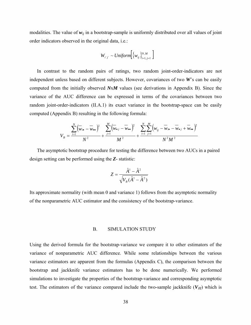
modalities. The value of wij in a bootstrap-sample is uniformly distributed over all values of joint
order indicators observed in the original data, i.e.:
[ ]MNjiijji wUniformW ,
1,1`` ~==
In contrast to the random pairs of ratings, two random joint-order-indicators are not
independent unless based on different subjects. However, covariances of two W’s can be easily
computed from the initially observed NxM values (see derivations in Appendix B). Since the
variance of the AUC difference can be expressed in terms of the covariances between two
random joint-order-indicators (II.A.1) its exact variance in the bootstrap-space can be easily
computed (Appendix B) resulting in the following formula:
( ) ( ) ( )22
1 1
2
21
2
21
2
MN
wwww
M
ww
N
wwV
N
i
M
jjiij
M
jj
N
ii
B
∑∑∑∑= =
••••
=
•••
=
••• +−−+
−+
−=
The asymptotic bootstrap procedure for testing the difference between two AUCs in a paired
design setting can be performed using the Z- statistic:
)ˆˆ(
ˆˆ21
21
AAV
AAZB −
−=
Its approximate normality (with mean 0 and variance 1) follows from the asymptotic normality
of the nonparametric AUC estimator and the consistency of the bootstrap-variance.
B. SIMULATION STUDY
Using the derived formula for the bootstrap-variance we compare it to other estimators of the
variance of nonparametric AUC difference. While some relationships between the various
variance estimators are apparent from the formulas (Appendix C), the comparison between the
bootstrap and jackknife variance estimators has to be done numerically. We performed
simulations to investigate the properties of the bootstrap-variance and corresponding asymptotic
test. The estimators of the variance compared include the two-sample jackknife (VJ2) which is
38

equivalent to that proposed by DeLong et al. [19], the one-sample jackknife (VJ1) which ignores
the distinction between normal and abnormal subjects; and biased (VWb) and unbiased (VW)
estimators suggested by Wieand et al. [18]. The simulations follow the general approach
described in Chapter III Section A. All figures illustrate the estimates computed for samples of
size of 40 normal and 40 abnormal subjects, correlation between ratings (ρ) of 0.4, shape
parameter (b) of 1 in both modalities. In addition, for Figure V.3.b the AUC of each modality is
set equal to 0.85.
Figure V.1 illustrates the average variance estimates and their relative biases (percent of
deviation from the empirical variance). The graph in Figure V.1.a indicates a strong decreasing
relationship between the variance and average AUC
Figure V.1 Expectations of the variance estimators Types of the variance estimators: Wb- Wieand (biased); W-Wieand (unbiased); J2-two-sample jackknife; J1-one-sample jackknife; B-bootstrap. Graph a): Average estimates of the variance; Graph b): Estimated relative bias of the estimates (percent of deviation from the empirical variance)
Figure V.1.b indicates that the bootstrap-variance (VB) has an upward bias that increases with
increasing underlying AUC. The commonly used two-sample-jackknife-variance (VJ2)
demonstrates similar properties and the trend in upward bias is less sharp than the trend for the
39

bootstrap-variance. On average, however, the bootstrap-variance is much closer to the
conventional estimator than to any other.
Figure V.2 Efficiency of the variance estimators Types of the variance estimators: Wb- Wieand (biased); W- Wieand (unbiased); J2-two-sample jackknife; J1-one-sample jackknife; B-bootstrap. Graph a): Relative variability of the estimates (relative to the bootstrap); Graph b): Relative efficiency of the estimates (relative to bootstrap)
Figure V.2.a illustrates how variance estimators differ with respect to their variability. From
this graph it can be seen that the variability of the bootstrap-variance (VB) is quite small and
uniformly superior to both jackknife estimators. The biased estimator (VWb) proposed by Wieand
et al. has uniformly lower variance than the bootstrap estimator and the unbiased estimator (VW)
has lower variance when AUC>85.
Since four out of five variance estimators demonstrate bias for some values of AUC we
compare their efficiencies by considering the ratio of the “mean squared errors” (MSEs). Figure
V.2.b demonstrates efficiencies of the estimators relative to that produced by the bootstrap
approach. The bootstrap-variance (VB) has the mean squared error that is lower than that of the
unbiased estimator (VW) when AUC is less than 0.85 and lower than that of the biased estimator
(VWb) proposed by Wieand et al. when AUC is less than 0.8. The efficiency of the bootstrap-
variance is consistently better than that of the conventional variance estimator (VJ2).
40
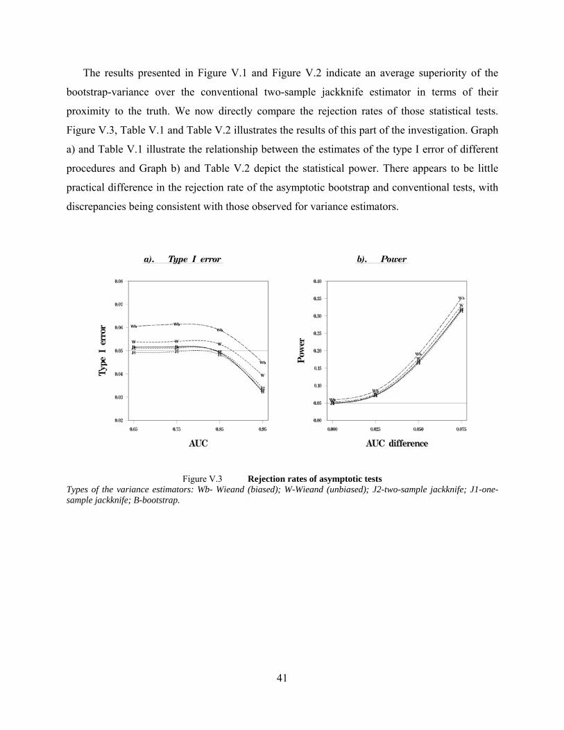
41
The results presented in Figure V.1 and Figure V.2 indicate an average superiority of the
bootstrap-variance over the conventional two-sample jackknife estimator in terms of their
proximity to the truth. We now directly compare the rejection rates of those statistical tests.
Figure V.3, Table V.1 and Table V.2 illustrates the results of this part of the investigation. Graph
a) and Table V.1 illustrate the relationship between the estimates of the type I error of different
procedures and Graph b) and Table V.2 depict the statistical power. There appears to be little
practical difference in the rejection rate of the asymptotic bootstrap and conventional tests, with
discrepancies being consistent with those observed for variance estimators.
Figure V.3 Types of the variance estimators: Wb- Wieand (biase knife; J1-one-sample jackknife; B-bootstrap.
Rejection rates of asymptotic tests d); W-Wieand (unbiased); J2-two-sample jack

42
Table V.1 Bootstrap asymptotic test: type I error
Sample size
N=20 normal M=20 abnormal
subjects N=40 normal M=40 abnormal
subjects N=60 normal M=60 abnormal
subjects
Correlation AUC The same
ROC Crossing
ROCs The same
ROC Crossing
ROCs The same
ROC Crossing
ROCs (b1=b2=1) (b1=1,b2=1/2) (b1=b2=1) (b1=1,b2=1/2) (b1=b2=1) (b1=1,b2=1/2)
J2 B J2 B J2 B J2 B J2 B J2 B
ρ=0.0 0.65 0.056 0.059 0.056 0.059 0.053 0.054 0.053 0.054 0.054 0.054 0.053 0.054 0.75 0.052 0.054 0.057 0.062 0.051 0.052 0.052 0.053 0.051 0.052 0.051 0.052 0.85 0.048 0.050 0.051 0.052 0.047 0.047 0.050 0.051 0.049 0.050 0.048 0.049
0.95 0.018 0.019 0.020 0.020 0.038 0.037 0.043 0.043 0.044 0.043 0.046 0.046
ρ=0.4 0.65 0.054 0.055 0.054 0.056 0.051 0.052 0.053 0.055 0.054 0.054 0.053 0.054 0.75 0.048 0.049 0.052 0.053 0.051 0.052 0.049 0.050 0.051 0.051 0.050 0.051 0.85 0.038 0.039 0.044 0.045 0.050 0.049 0.050 0.050 0.053 0.053 0.045 0.046 0.95 0.015 0.014 0.017 0.016 0.034 0.032 0.035 0.034 0.045 0.043 0.044 0.043
ρ=0.6 0.65 0.046 0.046 0.051 0.051 0.045 0.045 0.051 0.050 0.049 0.049 0.053 0.053 0.75 0.046 0.046 0.047 0.047 0.053 0.053 0.049 0.049 0.054 0.054 0.045 0.045 0.85 0.042 0.040 0.041 0.040 0.044 0.042 0.049 0.049 0.050 0.049 0.054 0.054 0.95 0.011 0.009 0.015 0.014 0.030 0.027 0.036 0.034 0.037 0.035 0.048 0.046
Types of the variance-estimators: J2-two-sample jackknife; B-bootstrap.
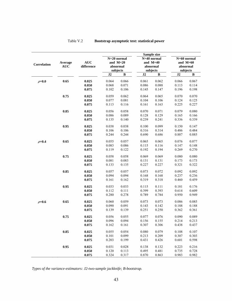
Table V.2 Bootstrap asymptotic test: statistical power
Sample size
Correlation Average AUC AUC
difference
N=20 normal and M=20 abnormal subjects
N=40 normal and M=40 abnormal subjects
N=60 normal and M=60 abnormal subjects
J2 B J2 B J2 B
ρ=0.0 0.65 0.025 0.064 0.066 0.061 0.062 0.066 0.067 0.050 0.068 0.071 0.086 0.088 0.113 0.114 0.075 0.102 0.106 0.145 0.147 0.196 0.198
0.75 0.025 0.059 0.062 0.064 0.065 0.070 0.070 0.050 0.077 0.081 0.104 0.106 0.124 0.125 0.075 0.113 0.116 0.161 0.163 0.225 0.227
0.85 0.025 0.056 0.058 0.070 0.071 0.079 0.080 0.050 0.086 0.089 0.128 0.129 0.165 0.166 0.075 0.135 0.140 0.239 0.241 0.336 0.339
0.95 0.025 0.038 0.038 0.100 0.099 0.150 0.147 0.050 0.106 0.106 0.316 0.314 0.486 0.484 0.075 0.244 0.244 0.690 0.686 0.887 0.885
ρ=0.4 0.65 0.025 0.055 0.057 0.065 0.065 0.076 0.077 0.050 0.083 0.086 0.115 0.116 0.147 0.148 0.075 0.119 0.122 0.192 0.194 0.269 0.270
0.75 0.025 0.058 0.058 0.069 0.069 0.080 0.080 0.050 0.081 0.083 0.131 0.131 0.173 0.173 0.075 0.133 0.135 0.227 0.227 0.321 0.322
0.85 0.025 0.057 0.057 0.073 0.072 0.092 0.092 0.050 0.094 0.094 0.168 0.168 0.237 0.236 0.075 0.161 0.162 0.319 0.318 0.460 0.459
0.95 0.025 0.033 0.033 0.115 0.111 0.181 0.176 0.050 0.112 0.111 0.399 0.393 0.614 0.609 0.075 0.280 0.278 0.789 0.784 0.950 0.949
ρ=0.6 0.65 0.025 0.060 0.059 0.073 0.073 0.086 0.085 0.050 0.090 0.091 0.143 0.142 0.188 0.188 0.075 0.139 0.139 0.251 0.250 0.362 0.361
0.75 0.025 0.056 0.055 0.077 0.076 0.090 0.089 0.050 0.096 0.094 0.156 0.155 0.214 0.213 0.075 0.162 0.161 0.307 0.306 0.438 0.437
0.85 0.025 0.055 0.054 0.080 0.079 0.108 0.107 0.050 0.101 0.099 0.213 0.209 0.307 0.303 0.075 0.203 0.199 0.431 0.426 0.601 0.598
0.95 0.025 0.031 0.028 0.138 0.132 0.223 0.216 0.050 0.120 0.113 0.495 0.481 0.735 0.728 0.075 0.324 0.317 0.870 0.863 0.983 0.982
Types of the variance-estimators: J2-two-sample jackknife; B-bootstrap.
43

C. SUMMARY AND DISCUSSION
We have derived a closed-form solution for the bootstrap-variance of the nonparametric
estimator of AUC difference. Availability of such an estimator allows for construction of an
easy-to-implement asymptotic bootstrap test as well as alleviating the computational burden.
The results of our simulation study indicate that the bootstrap-variance provides a good
estimate of the true variability. Among the estimators we considered it is the most efficient for
AUCs lower than 0.8 but less efficient than both estimators proposed by Wieand et al. [18] for
larger AUCs. The bootstrap estimator also has an upward bias which increases with increasing
average AUC. Compared to the conventional two-sample-jackknife [19] the bootstrap estimator
of the variance is more efficient but has greater bias for large AUCs (>0.85). Both estimators
proposed by Wieand et al. [18] perform well. The biased estimator has lower mean squared error
(MSE) than that of the bootstrap-variance for AUC>0.80 and the unbiased version of the
estimator has lower MSE for AUC>0.85 (the low MSE of the biased estimator is perhaps due to
its low variance).
For small AUCs the asymptotic bootstrap test, compared to the conventional procedure, has
even more elevated type I error and, perhaps because of that, is slightly more powerful. For large
AUCs the bootstrap-based test is more conservative than the conventional test implying even
greater potential for the loss of the statistical power. Thus, although the bootstrap might offer a
better way to estimate the variability than the conventional two-sample jackknife approach it
leads to an asymptotic test with slightly inferior small-sample properties. However, our
simulations indicate no practical difference between bootstrap and conventional test.
44
VI. CONDITIONAL TEST
In this chapter we develop a novel approach for statistical comparison of the overall performance
of the two modalities in a paired design setting. The motivation for this approach was dependent
on two factors. First, the AUC can be viewed as a simple function of the relative orderings of all
pairs of normal and abnormal subjects. Secondly, the difference in the AUCs for two modalities
in a paired design depends only on those pairs where the relative orderings of normal and
abnormal cases differ. The corresponding statistical test is similar in spirit to McNemar’s
procedure [44] which conducts the analysis only on discordant pairs. Simulations are conducted
to verify the small-samples properties of the conditional test. This part of the research is
published in Academic Radiology [33].
A. CONDITIONAL APPROACH
In general, the ratings assigned to a randomly selected pair of normal and abnormal cases can
only be in one of three possible orderings: YX < , YX = , YX > (i.e. normal case having score
lower than, equal to, or higher than the score for the abnormal case). Each of these possibilities
represents different degrees to which a modality (including the observer) can distinguish between
a given set of actually positive and actually negative findings, namely:
- the modality correctly discriminates between given cases; YX <
- the modality does not discriminate between given cases; YX =
YX > - the modality incorrectly discriminates the between given cases.
In a paired design when the same cases are evaluated by two modalities the nine possible
joint orderings between the ratings of the normal and abnormal cases can be classified as
follows:
45

(VI.A.1)
In the table above, the ‘+’ indicates a combination of orderings implying the 1st modality is
superior to the 2nd, ‘-’ indicates a combination of orderings implying the 2nd modality is superior
to the 1st modality, and “0” indicates a combination of orderings suggesting equivalence between
the two modalities with respect to their ability to correctly discriminate between cases with and
without the abnormality. In this work the orderings (‘+’ or ‘-’) that contribute to the
determination of which modality is superior are naturally termed “discordant” orderings while
the others (‘0’) are termed “concordant”.
The overall ability of the modality to identify the abnormality can be viewed as the AUC.
The difference between the overall performance levels of two modalities can therefore be
summarized as the difference between two AUCs:
(VI.A.2)
00
0
11
11
11
222222
−−>+−=++<>=<
YXYXYX
YXYXYX
( ) ( ) ( ) ( )22212211
211121 YXPYXPYXPYXPAA =−<−=+<=−
The estimator of the difference above is written in terms of probabilities of “marginal”
orderings (orderings that corresponds to rows and columns of table VI.A.1). Alternatively, in a
paired design setting we can express this difference in terms of probabilities of discordant joint
orderings. Namely, by replacing each probability of the “marginal” ordering in VI.A.2 with the
sum of joint probabilities (probabilities of corresponding cells in table VI.A.1) and canceling
common terms, one obtains the following expression directly:
(VI.A.3)( ) ( ) ( )( ) ( ) ( )1122
211122
211122
2211212211
21221121
,,,
,,,
YXYXPYXYXPYXYXP
YXYXPYXYXPYXYXPAA
>=−=<−><−
>=+=<+><=−
In any given dataset, the probabilities of the joint discordant orderings contain all the needed
information in order to quantify the differences in the area under the two ROC curves orderings.
Motivated by this observation we construct a statistical test conditional on the pairs of cases with
observed discordant orderings.
Note that for truly continuous ratings (i.e. when no ties are possible) the difference between
two AUC in a paired design can be equivalently written as:
( ) ( )1122221121 ,, YXYXPYXYXPAA ><−><=−
Since, in the continuous case:
46

),(),(:),( 22112211 YXYXorYXYXYXD <>><=
then:
( ) ( )( ) 1),(|2
),(|),(|11
221121
−∈<=
=∈<−∈<=−
DYXYXPDYXYXPDYXYXPAA
and the hypothesis of equality between two AUCs is equivalent to the hypothesis:
( ) 2111 ),(| =∈< DYXYXP .
B. CONDITIONAL PERMUTATION TEST
The test we propose makes use of a nonparametric estimator of the AUC difference and is based
on the concept of estimating the variability of the sum of discordant order indicators (structural
elements of the nonparametric AUC difference estimator). Namely, in the underlying sample
space the initial discordant orderings may correspond to a different “degree” (level) of
superiority of one of the modalities. In this sample space we estimate the variability of the sum
of discordant ordering indicators:
(VI.B.1) ∑≠
=0w:j,i
ijij
WW
Note that the quantity Wij as defined in (II.A.3) differentiates the possible orderings for the
pair of ith normal and jth abnormal cases (VI.A.1) in the following manner:
(VI.B.2)
010
10
2111
21
2111
2111
222222
−−>−=
<>=<
ji
ji
ji
jijijiij
YXYXYX
YXYXYXW
We propose conditioning on the set of discordant orderings, D. (non-zero Wij in the data
remain non-zero for all permutations). The variance of W can be expressed through the variances
of each of the Wij and the covariances between any pair of these. Thus, to compute the variance
of the W we need moments of the joint distribution of any pair of ijW . To obtain these moments
we model the marginal joint distribution of any pair of ijW .
47

ijWAlthough, in general the joint distribution of any pair of is difficult to derive, the use of
the permutation test provides a direct way to estimate the needed distributions [32]. Following
the approach used in [24] the rank-ratings (ranks of the rating) are used to generalize the
inferences to a situation where the two modalities may have different underlying rating scales. If
the two modalities are assumed to have the same underlying scales the actual ratings (not the
rank ratings) should be used. The basic permutation space Ω is created by permuting the case-
specific rank-ratings between the two modalities within the structure of given pairs.
Thus, if for the pair consisting of the ith normal case and the jth abnormal case we observe
rank-ratings of xi1 and yj
1 for the first modality and xi2 yj
2 for the second modality then the four
permutations within this paired structure are:
where the first pair is assumed to be observed for the first modality and the second pair is
assumed to be observed for the second modality. We are assuming that under the null hypothesis
the ranks for normal (abnormal) cases satisfy the statistical assumption of exchangeability
implying that each of these four situations is equally likely. Let
)y,x(,)y,x(
)y,x(,)y,x(
)y,x(,)y,x(
)y,x(,)y,x(
1j
1i
2j
2i
1j
2i
2j
1i
2j
1i
1j
2i
2j
2i
1j
1i
2,2
1q,1pq,p
ijw==
sociated with the i
be the score as
assigned in II.A.3 for each of the four possible permutations as th normal and jth
abnormal pair of cases. The value represents the value of Wij associated with the observed
data. A superscript of p=2 (q=2) corresponds to a permutation where the normal (abnormal)
rank-ratings of the two modalities are interchanged.
Assuming equal probability of each permutation under the null hypothesis, each Wij is
uniformly distributed over the values
11ijw
2,2
1q,1pq,p
ijw==
which belong to the set 1,,0,,1 21
21−− and
possess the anti-symmetric property: .
The pairs of normal and abnormal cases with initially observed discordant order of ratings
are distinguished by the condition and the random quantity in VI.B.1 can be written as:
21ij
12ij
22ij
11ij ww,ww −=−=
0w11ij ≠
48

∑≠
=0w:j,i
ij11ij
WW .
Constraining the discordant orderings to remain discordant (i.e. conditioning on D) results in
Wij that are uniformly distributed over non-zero values from 2,2
1q,1pq,p
ijw==
.
The set of values can be obtained by determining the relative orderings
al case and then taking the differences in a
manner consistent with II.A.3. The moments of the
2,2,M,N
1q,1p1j,1iq,p
ijw====
between rank-ratings for every normal and abnorm
0w:j,iij 11
ijW
≠ can be computed from the set of
values using the formulae shown in the Appendix D. Finally, to implement the
lity of AUC between two modalities in a paired design we propose
comp
2,2,M,N
1q,1p1j,1iq,p
ijw====
conditional test of equa
aring the statistic ( )DWVar
W|Ω
to the pre-specified normal percentile.
C. SIMULATION STUDY
To verify the validity of the proposed test we performed simulations to investigate its type I error
for different underlying AUCs, correlations between case ratings across modalities and different
sample sizes. In our simulations we assume equal correlation across modalities for the ratings of
normal and abnormal cases and consider scenarios with non-crossing as well as crossing ROC
curves.
The general protocol of simulations follows the general approach described in Chapter II,
Section A. In addition to simulations of conventional datasets, we conducted simulations where
the samples from the binormal distribution (“typical” cases) were enriched with “easy” and
“difficult” cases. Such enrichment has the practical effect of increasing the number of concordant
pairs (i.e. pairs where there is an agreement for both modalities). When the concordance level is
high the method by DeLong et al. has been shown to have a below nominal level (0.05) type I
error [Chapter III,31]. Hence in these situations the conventional nonparametric test may have
unnecessarily low statistical power.
49

50
The ratings of “easy” and “difficult” cases were defined relative to the ratings of cases in the
other groups. Namely, “easy” normal cases are rated by both modalities below that of any
“typical” abnormal cases but might be higher than some of the “difficult” abnormal cases; the
“difficult” normal cases are those rated by both modalities higher than the “typical” abnormal
cases but might be rated lower than “easy” abnormal cases; and the “typical” normal and
abnormal cases have generally overlapping range of ratings. The fixed number of cases of each
type was simulated from normal distributions in a manner that easy normal/abnormal cases had
the same distributions as difficult abnormal/normal cases (e.g. completely missed abnormal cases
were considered to be rated similar to easy normal cases). The distributions of easy and difficult
cases were sufficiently different than the distribution for typical cases to prevent overlapping.
Table VI.1 illustrates that the rejection rate of the proposed procedure is generally close to
the nominal level of 0.05 while being conservative for small sample sizes, large AUCs, and high
correlation between ratings of the same case.

51
Table VI.1 Conditional test: rejection rate
N=20 normal and M=20 abnormal subjects N=40 normal and M=40 abnormal
subjects N=60 normal and M=60 abnormal subjects
AUC
ρ=0.0 ρ=0.2 ρ=0.4 ρ=0.6 ρ=0.0 ρ=0.2 ρ=0.4 ρ=0.6 ρ=0.0 ρ=0.2 ρ=0.4 ρ=0.6
0.60 0.042 0.041 0.041 0.038 0.045 0.043 0.046 0.045 0.049 0.050 0.049 0.048 0.65 0.043 0.040 0.040 0.039 0.046 0.046 0.046 0.044 0.050 0.050 0.049 0.049 0.70 0.042 0.041 0.040 0.038 0.046 0.046 0.046 0.043 0.047 0.049 0.048 0.048 0.75 0.041 0.038 0.038 0.036 0.046 0.046 0.045 0.043 0.047 0.046 0.046 0.046 0.80 0.040 0.038 0.036 0.034 0.046 0.046 0.045 0.044 0.048 0.048 0.047 0.044 0.85 0.036 0.036 0.034 0.030 0.043 0.043 0.043 0.045 0.047 0.047 0.048 0.045 0.90 0.033 0.031 0.029 0.025 0.042 0.041 0.040 0.040 0.046 0.045 0.045 0.043
The same ROC
(b1=b2=1)
0.95 0.018 0.017 0.015 0.015 0.036 0.036 0.033 0.033 0.043 0.043 0.040 0.040
0.60 0.047 0.047 0.045 0.043 0.051 0.051 0.050 0.050 0.052 0.050 0.051 0.052 0.65 0.047 0.044 0.043 0.043 0.050 0.049 0.049 0.048 0.051 0.051 0.052 0.053 0.70 0.047 0.044 0.042 0.041 0.051 0.051 0.050 0.049 0.052 0.051 0.052 0.052 0.75 0.046 0.043 0.044 0.039 0.051 0.049 0.049 0.048 0.052 0.052 0.052 0.051 0.80 0.044 0.041 0.040 0.038 0.050 0.048 0.050 0.049 0.052 0.051 0.049 0.050 0.85 0.041 0.039 0.037 0.035 0.050 0.048 0.048 0.049 0.051 0.050 0.049 0.049 0.90 0.035 0.034 0.030 0.028 0.048 0.048 0.047 0.048 0.049 0.049 0.047 0.046
Crossing ROC
( b1=1, b2=1/2)
0.95 0.018 0.017 0.016 0.015 0.040 0.040 0.040 0.040 0.045 0.046 0.044 0.043

We also compared the power of the proposed conditional procedure to that of the
conventional nonparametric procedure developed by DeLong et al. [19]. For the binormal
(“typical” cases only) datasets the conventional AUC test is somewhat more powerful than the
conditional procedure. For example, for 20 normal and 20 abnormal cases that form non-crossing
ROC curves with AUCs of 0.75 and 0.85, and a correlation of 0.4 between ratings on the same
cases, the conventional AUC test has power and type I error correspondingly of 0.223 and 0.046
as compared with 0.191 and 0.036 for the conditional procedure proposed here. However, the
presence of small number of “easy” and “difficult” cases may result in an advantage for the
proposed conditional test in datasets with 20 “typical” normal and 20 “typical” abnormal cases.
The estimates of the power for the two procedures in “enriched” datasets are presented in Table
VI.2.
Table VI.2 Conditional test: statistical power in the “enriched” datasets
ρ=0.0 ρ=0.2 ρ=0.4 ρ=0.6 Average AUC
AUC difference DeLong Conditional DeLong Conditional DeLong Conditional DeLong Conditional
0.75 0.1 0.118 0.122 0.129 0.136 0.151 0.162 0.191 0.209 0.2 0.380 0.394 0.436 0.454 0.526 0.545 0.658 0.685
0.8 0.1 0.128 0.135 0.143 0.153 0.167 0.181 0.208 0.233 0.2 0.441 0.463 0.503 0.527 0.583 0.611 0.712 0.742
0.85 0.1 0.148 0.161 0.165 0.181 0.189 0.211 0.244 0.275 0.2 0.537 0.576 0.597 0.634 0.671 0.713 0.773 0.816
“Enriched” datasets include: 20” typical” normal + 20 “typical” abnormal, 10 “easy” normal + 10 “easy” abnormal and 3 “difficult” normal +3“difficult” abnormal subjects.
D. SUMMARY AND DISCUSSION
The proposed procedure illustrates a conceptually new approach to testing the equality of overall
diagnostic performances between two modalities in a paired design setting. Using the nature of a
paired design and relative orderings we introduced the idea of concordances and discordances in
the task of comparing overall performances of diagnostic systems. Conditioning on the
discordant order indicators resulted in a test similar in spirit to McNemar’s test. However the
52

complex correlation structure of the discordant order indicators prevents construction of an exact
procedure and greatly complicates the process of developing an asymptotic test. The estimator of
the variance used in our method is derived using the assumption of exchangeability of the case-
specific rank-ratings under the null hypothesis. The condition of exchangeability is stricter than
the condition of equality of AUCs and implies an equality of the two ROC curves. However, our
computer simulations indicate that the rejection rate of the proposed test remains close to
nominal significance level even in cases of substantially crossing ROC curves (b1=1, b2=1/2), at
least for moderate sample sizes, hence rejection of the null hypothesis is unlikely to occur unless
there is a difference in the AUCs.
A substantial number of concordances may occur in a screening population where there may
be a substantial number of “easy” or “difficult” cases or in laboratory experiments where the
method of selection of cases could result in a higher level of concordance. In datasets with
ratings that can be monotonically transformed to a binormal distribution the number of
“concordant” orderings increases with increasing AUC and correlation between ratings in
different modalities. This may explain in part the conservative behavior of the conventional
nonparametric AUC test [19]. It should be noted however that the impact of “concordant”
orderings on the efficiency of the conditional procedure is most evident for reasonably small
sample sizes (less than 60 normal and 60 abnormal).
In conclusion, we presented a conceptually new approach to the assessment of differences
between two diagnostic modalities in a paired design. This method, which is conditioned on
discordances in discrimination between normal and abnormal cases in the two modalities, may
provide advantages in relatively small studies where the selection of cases results in a high level
of concordance.
53
VII. CONCLUSIONS AND DISCUSSION
In this work we investigated the effects of various parameters on the small-sample properties of
the conventional nonparametric procedure for comparing correlated AUCs and developed three
novel nonparametric approaches for comparing two diagnostic modalities in a paired design
setting. The conducted research provides important information and methods that can be useful
for study design and choice of an appropriate statistical method for analysis. Also the proposed
statistical approaches create a solid foundation for further development of nonparametric
methods and the results of simulation studies may offer guidelines for more complex scenarios.
In our study of the properties of the conventional procedure for nonparametric comparison of
the correlated AUCs we attempted to characterize the effect of various parameters on the
statistical hypothesis testing with small samples. For each parameter we described the direction
and relative magnitude of the effect on the type I error and power of a statistical test. The
parameters we identified as having an effect are (in decreasing order of influence): average AUC
(A), correlation between modalities (ρ), and the prevalence of abnormal subjects in the selected
sample (p).
The proposed permutation procedure for comparing two diagnostic systems provides the
ability to perform the exact test for small samples and the asymptotic test for larger ones. The
easy-to-implement asymptotic test offers an excellent approximation of the exact procedure even
for sample sizes as low as 6 normal and 6 abnormal subjects. The quality of approximation can
be attributed in part to the exact nature of the variance-estimator used in the construction of the
asymptotic test and to the symmetry of the permutation distribution of the nonparametric
estimator of AUC difference. The developed procedure is based on all permutations of the
subject specific rank ratings and is formally a test for equality of ROC curves that is sensitive to
the alternatives of AUC difference. For small samples and for underlying parameters that are
common in experimental studies in the field of diagnostic test evaluation (AUC of more than
54
0.75, correlation of more than 0.4) the permutation test possesses good operating characteristics
and is more powerful than the conventional nonparametric procedure for AUC comparisons.
Exploiting the properties of the nonparametric estimator of AUC difference we derived a
closed-form solution for the bootstrap-variance and constructed an easy-to-implement
asymptotic test. The results of our simulation study indicate that the bootstrap-variance is
uniformly more efficient than the conventional two-sample-jackknife estimator; however it has a
higher bias for large AUCs. Also for small AUCs the bootstrap-variance was shown to have a
relatively small bias and the best efficiency among considered estimators. It is worth noting that
we measure the efficiency by the “mean squared error” (MSE) what induces a specific type of
tradeoff between bias and variability; hence it is possible that under a different measure (for
instance absolute instead of squared distance) the relative efficiencies of the estimators will
change. Despite its good properties the bootstrap variance leads to an asymptotic test with small-
sample properties slightly inferior to that of the conventional procedure developed by DeLong et
al. [19]. In conclusion, for the nonparametric estimator of the AUC difference, the bootstrap
approach might offer a better estimator of the variability than the conventional two-sample
jackknife procedure; however it does not produce a better asymptotic test.
Using the relationship of the AUC difference to the relative orderings of the ratings assigned
to pairs of normal and abnormal subjects by two modalities we introduced the concept of
concordances and discordances in the task of comparing overall performances of diagnostic
systems with paired data. Conditioning on the discordant order indicators resulted in a test
similar in spirit to McNemar’s test. However the complex correlation structure of the discordant
order indicators prevents construction of an exact procedure and greatly complicates the process
of developing an asymptotic test. The problem of constructing the asymptotic test was solved
with the help of the previously developed permutation test. The type I error of the procedure for
small samples was verified using computer simulations. The conditional nonparametric test
presented here is an alternative approach to existing unconditional procedures and may offer
statistical advantages in the presence of highly concordant data.
In developing the permutation approach we have restricted our attention to comparing two
diagnostic modalities with paired data where the primary summary statistic is the area under the
ROC curve. As mentioned previously the permutation approach can be applied to the comparison
55
of two diagnostic systems evaluated on independent datasets as well. Furthermore, if the data is
paired but incomplete, our test could be modified using an approach similar to the one proposed
by Zhou and Gatsonis [29] for correcting the conventional approach of DeLong et al. [19]. The
permutation approach can also be applied either when different methods of estimating the area
under the ROC curve are employed or when different summary statistics are used [7,8,14,24].
Although the permutation test might be used with various test statistics the computation time for
the exact test might increase for some of them. Furthermore it may be impossible to derive exact
permutation moments as was done for the nonparametric estimator of the difference in AUCs
and thus there may be no simple approximation to the exact test.
An alternative summary statistic that is often used is the partial area under the ROC curve
[20,28]. In theory, the permutation approach could be applied to this summary statistic although
several issues need to be addressed. Some of these issues are discussed in [28] where the authors
attempted to compare the partial areas under two ROC curves by modifying the conventional
approach of DeLong et al. [19].
The permutation approach we have used might be also applicable to a more general approach
of comparing diagnostic systems than ROC curve analysis. Bunch et al. [45] proposed a Free-
response Receiver Operating Characteristic (FROC) curve which describes the task of detection
and localization of multiple abnormalities per image. Although some work has been done
addressing the comparison of FROC curves [46,47], the statistical methodology has been much
less developed than for ROC curves. The permutation approach could circumvent some of the
problems encountered in FROC analysis such as potential correlation between the multiple
observations per image.
Other directions of future research include extension of the proposed procedures to
accommodate the “multiple-reader” setting – a commonly used design in which several readers
evaluate selected cases using different modalities. The random effects models in the multiple-
reader settings offer another area of possible development [34,35,36,37].
56
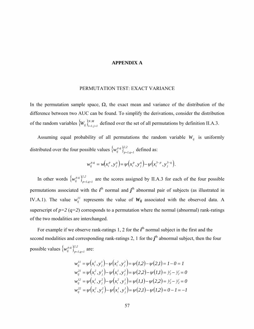
APPENDIX A
PERMUTATION TEST: EXACT VARIANCE
In the permutation sample space, Ω, the exact mean and variance of the distribution of the
difference between two AUC can be found. To simplify the derivations, consider the distribution
of the random variables defined over the set of all permutations by definition II.A.3.
Assuming equal probability of all permutations the random variable is uniformly
distributed over the four possible values
M.N1j,1iijW
==
ijW
2,2
1q,1pq,p
ijw==
defined as:
( ) ( ) ( )q3j
p3i
qj
pi
qj
pi
q,pij y,xy,xy,xww −−−== ψψ .
In other words are the scores assigned by II.A.3 for each of the four possible
permutations associa ith normal and jth abnormal pair of subjects (as illustrated in
IV.A.1). The value represents the value of Wij associated with the observed data. A
superscript of p=2 (q=2) corresponds to a permutation where the normal (abnormal) rank-ratings
of the two modalities are interchanged.
For example if we observe rank-ratings 1, 2 for the ith normal subject in the first and the
second modalities and corresponding rank-ratings 2, 1 for the jth abnormal subject, then the four
possible values are:
2,2
1q,1pq,p
ijw==
ted with the 11ijw
2,2
1q,1pq,p
ijw==
( ) ( ) ( ) ( )( ) ( ) ( ) ( )( ) ( ) ( ) ( )( ) ( ) ( ) ( ) 1102,11,2y,xy,xw
02,21,1y,xy,xw
01,12,2y,xy,xw
1011,22,1y,xy,xw
1j
1i
2j
2i
22ij
21
211
j2i
2j
1i
12ij
21
212
j1i
1j
2i
21ij
2j
2i
1j
1i
11ij
−=−=−=−=
=−=−=−=
=−=−=−=
=−=−=−=
ψψψψ
ψψψψ
ψψψψ
ψψψψ
57

Note also that the set naturally possesses certain anti-symmetric properties,
namely:
2,2
1q,1pq,p
ijw==
211222112
12
1, ,,1,,0,,12,1,,...,1,,...,1 ijijijijqp
ij wwwwwqpMjNi −=−=−−∈=∀==∀ .
The values for each pair of normal-abnormal subjects 2,2
1q,1pq,p
ijw==
2,2,M,N
1q,1p1j,1iq,p
ijw====
can be
obtained by comparing each available rank-rating for a normal subject with the rank-ratings of
every abnormal one using II.A.3.
Thus, the distribution of can be summarized as: ijW
( ) 2,1q,pwWPw,w,w,wWM,...,1j;N,...,1i 41q,p
ijij22ij
21ij
12ij
11ijij =∀==∈==∀ .
The joint distribution of any two with the same subscripts follows naturally from II.A.3
and the permutation algorithm. For example, the joint distribution of Ws sharing the same
normal subjects ( ) can be summarized as follows:
ijW
ijW , ilW
[ ] 2,1,,),(),(
),(),,(),,(),,(
),,(),,(),,(),,(),(;,...,1;,...,1
81,,
2222212222212121
1212111212111111
=∀==
⎪⎭
⎪⎬⎫
⎪⎩
⎪⎨⎧
∈≠==∀
oqpwwWWP
wwwwwwww
wwwwwwwwWWjlMjNi
opil
qpijilij
ilijilijilijilij
ilijilijilijilijilij
We can now derive the mean and covariance structure of the set of the random variables
. These are as follows: M,N1j,1iijW
==
, jl;ik;M,...,1l,j;N,...,1k,i ≠≠==∀
( ) ( )0
44/)(
211222112
1
2
1
, =+++
===••
= =Ω ∑∑ ijijijij
ijp q
qpijij
wwwwwwWE ,
( ) ( ) ( )∑∑= =
+==−=
2
1p
2
1q
212ij
211ij
2q,pij2
ij2
ijij 2ww
4w
)W(E)W(E)W(Var ΩΩΩ ,
and
=−= )W(E)W(E)WW(E)W,W(Cov ilijilijilij ΩΩΩΩ
58

( ) ( ) ••
= =
−
×=+×+
=+
= ∑∑11
121112112
1
2
1
3,,,,
48ilij
ililijij
p q
qpil
qpij
qpil
qpij ww
wwwwwwww
=−= )W(E)W(E)WW(E)W,W(Cov kjijkjijkjij ΩΩΩΩ
( ) ( ) 11211121112
1
2
1
,3,,,
48••
= =
−
×=+×+
=+
= ∑∑ kjijkjkjijij
p q
qpkj
qpij
qpkj
qpij ww
wwwwwwww
0)W,W(Cov klij =Ω .
Using the derived formulae for the moments of M,N1j,1iijW
==, the moments of the estimator of
the difference between AUC in Ω are as follows:
0NM
)W(E)AA(E
N
1i
M
1jij
21 ==−∑∑= =
Ω
Ω
( ) ( ) ⎜⎜⎜
⎝
⎛++=
⎟⎟⎠
⎞⎜⎜⎝
⎛
=− ∑∑∑∑∑∑∑
= =≠== =
= =N
1i
M
1j
M
jl,1l
ilij
N
1i
M
1jij22
N
1i
M
1jij
21 )W,W(Cov)W(VarNM
1NM
WVar)AA(Var ΩΩ
Ω
Ω
=⎟⎟⎟
⎠
⎞++ ∑∑∑∑∑∑∑
= =≠=
≠== =
≠=
N
1i
M
1j
N
ik,1k
M
jl,1l
klij
M
1j
N
1i
N
ik,1k
kjij )W,W(Cov)W,W(Cov ΩΩ
( )( ) ( ) ( ) ( ) =
⎟⎟⎟
⎠
⎞
⎜⎜⎜
⎝
⎛×+×+
+= ∑∑∑ ∑∑∑∑∑
= =≠= = =
≠=
••••
= =
N
i
M
j
M
jll
M
j
N
i
N
ikk
kjijilij
N
i
M
j
ijij wwwwww
NM 1 1 ,1 1 1 ,1
1111
1 1
212211
2 21
( )( ) ( ) ( ) ( ) ( ) ( ) ⎟
⎟⎠
⎞⎜⎜⎝
⎛
⎭⎬⎫
⎩⎨⎧
−+⎭⎬⎫
⎩⎨⎧
−++= ∑∑∑∑∑∑∑∑= =
•
=
••
= =
•
=
••
= =
M
j
N
iij
M
jj
N
i
M
jij
N
ii
N
i
M
jijij wwNwwMww
NM 1 1
21
1
212
1 1
21
1
212
1 1
2122112 2
11
( )( ) ( )
( ) ( )2
1
21
21
21
1
212
1
2122
1M
w
N
wwNwM
NM
M
jj
N
iiM
jj
N
ii
∑∑∑∑ =
••
=
••
=
••
=
•• +=⎟⎟
⎠
⎞⎜⎜⎝
⎛+= .
59
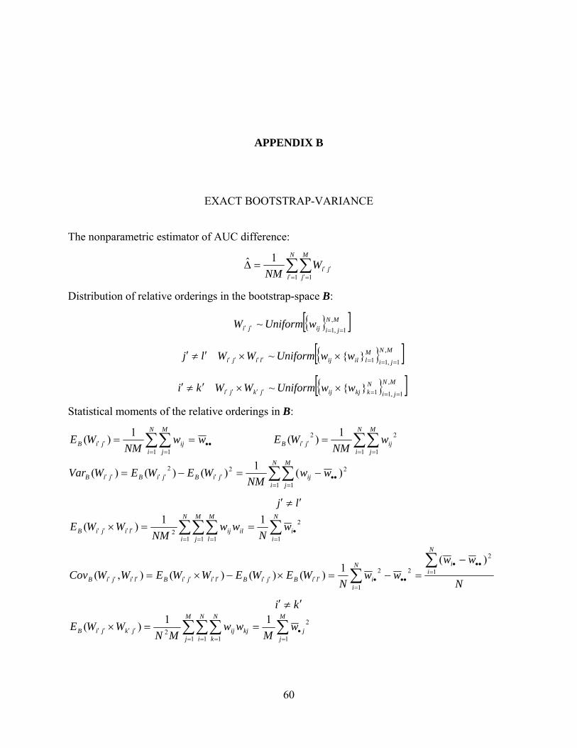
APPENDIX B
EXACT BOOTSTRAP-VARIANCE
The nonparametric estimator of AUC difference:
∑∑=′ =′
′′=∆N
i
M
jjiW
NM 1 1
1ˆ
Distribution of relative orderings in the bootstrap-space B:
[ ]MNjiijji wUniformW ,
1,1~
==′′
[ ]MN
jiMlilijliji wwUniformWWlj ,
1,11~===′′′′ ××′≠′
[ ]MN
jiNkkjijjkji wwUniformWWki ,
1,11~===′′′′ ××′≠′
Statistical moments of the relative orderings in B:
∑∑= =
••′′ ==N
i
M
jijjiB ww
NMWE
1 1
1)( ∑∑= =
′′ =N
i
M
jijjiB w
NMWE
1 1
22 1)(
∑∑= =
••′′′′′′ −=−=N
i
M
jijjiBjiBjiB ww
NMWEWEWVar
1 1
222 )(1)()()(
lj ′≠′
∑∑∑∑=
•= = =
′′′′ ==×N
ii
N
i
M
j
M
lilijlijiB w
Nww
NMWWE
1
2
1 1 12
11)(
N
wwww
NWEWEWWEWWCov
N
iiN
iiliBjiBlijiBlijiB
∑∑ =
•••
••=
•′′′′′′′′′′′′
−=−=×−×= 1
2
2
1
2)(
1)()()(),(
ki ′≠′
∑∑∑∑=
•= = =
′′′′ ==×M
jj
M
j
N
i
N
kkjijjkjiB w
Mww
MNWWE
1
2
1 1 12
11)(
60

M
www
M
wWEWEWWEWWCov
M
jj
M
jj
jkBjiBjkjiBjkjiB
∑∑=
•••
••=
•
′′′′′′′′′′′′
−=−=×−×= 1
2
21
2 )()()()(),(
Using the derived moments the bootstrap-variance of the nonparametric estimator of AUC
difference can be computed in closed form:
=⎭⎬⎫
⎩⎨⎧
++=∆ ∑∑ ∑∑∑ ∑∑∑=′ =′ =′ =′ ′≠′ =′ =′ ′≠′
′′′′′′′′′′
N
i
M
j
N
i
M
j jl
M
j
N
i ikjkjiBlijiBjiBB WWCovWWCovWVar
MNV
1 1 1 1 1 122 ),(),()(1)ˆ(
=
⎪⎪⎭
⎪⎪⎬
⎫
⎪⎪⎩
⎪⎪⎨
⎧
−−
+−−
+−
= ∑ ∑∑∑
= =••••••
= =•• N
i
M
jji
N
i
M
jij
wwMNMNww
NMNM
NM
wwNM
MN 1 1
221 1
2
22 )()1()()1()(
1
∑ ∑∑∑= =
••••••= =
•• −−
+−−
+−=N
i
M
jji
N
i
M
jij ww
NMNww
MNMww
MN 1 1
22
22
1 1
222 )()1()()1()(1
Note that
∑∑∑ ∑∑∑=
•••= = =
•••••••= =
•• −+−++−−=−M
jj
N
i
M
j
N
iijiij
N
i
M
jij wwNwwMwwwwww
1
2
1 1 1
22
1 1
2 )()()()(
Finally
221 1
2
21
2
21
2 )()()()ˆ(
MN
wwww
M
ww
N
wwV
N
i
M
jjiij
M
jj
N
ii
B
∑∑∑∑= =
••••=
•••=
•••+−−
+−
+−
=∆
61

APPENDIX C
VARIANCE ESTIMATORS OF THE AUC DIFFERENCE
Bootstrap-variance:
( ) ( ) ( )22
1 1
2
21
2
21
2
MN
wwww
M
ww
N
wwV
N
i
M
jjiij
M
jj
N
ii
B
∑∑∑∑= =
••••=
•••
=••• +−−
+−
+−
=
Biased variance-estimator proposed by Wieand et al.
( ) ( ) ( )22
1 1
2
21
2
21
2
11MN
wwww
M
ww
NN
N
ww
MMV
N
i
M
jjiij
M
jj
N
ii
Wb
∑∑∑∑= =
••••
=
•••
=
••• +−−−
−−
+−
−=
Unbiased variance-estimator proposed by Wieand et al.
( ) ( ) ( ))1)(1()1()1(
1 1
2
1
2
1
2
−−
+−−−
−
−+
−
−=
∑∑∑∑= =
••••
=
•••
=
•••
MNNM
wwww
MM
ww
NN
wwV
N
i
M
jjiij
M
jj
N
ii
W
Two-sample jackknife (DeLong et al.)
( ) ( ))1()1(
1
2
1
2
2 −
−+
−
−=
∑∑=
•••
=
•••
MM
ww
NN
wwV
M
jj
N
ii
J
One-sample jackknife
( ) ( )MN
MNM
ww
N
wwV
M
jj
N
ii
J +−+
×
⎥⎥⎥⎥
⎦
⎤
⎢⎢⎢⎢
⎣
⎡
−
−+
−
−=
∑∑=
•••
=
•••1
)1()1( 21
2
21
2
1
62

Certain deterministic relationships exist between considered variance-estimators:
(C.1)
These inequalities can be proved by the following observations:
BWb
JJWWb
VVVVVV
≤≤≤≤ 12
WWb VMN
NMV =−−
×)1)(1(
, hence WWb VV ≤
( )2
1 1
2
)1)(1( J
N
i
M
jjiij
W VMNNM
wwwwV =
−−
+−−+∑∑= =
••••
hence 2JW VV ≤
To establish relationship Note that: 12 JJ VV ≤
=
⎥⎥⎥⎥
⎦
⎤
⎢⎢⎢⎢
⎣
⎡
−
−
−+
−
−
−×
+−+
=∑∑=
•••=
•••
)1(
)(
1)1(
)(
11 1
2
1
2
1 MM
ww
MM
NN
ww
NN
MNMNV
M
ll
N
kk
J
⎥⎥⎥⎥
⎦
⎤
⎢⎢⎢⎢
⎣
⎡
−
−
−+−+
+
⎥⎥⎥⎥
⎦
⎤
⎢⎢⎢⎢
⎣
⎡
−
−
−+−+
=∑∑=
•••=
•••
)1(
)(
)1)(()1(
)1(
)(
)1)(()1( 1
2
1
2
MM
ww
MMNMMN
NN
ww
NMNNMN
M
ll
N
kk
1)1)((
)1(2
2
>−−+
−+=
−+−+
MNNMNNNMN
NMNNMN and 1
)1)(()1(
2
2
>−−+
−+=
−+−+
NMNMMMNMM
MMNMMN Since
12 JJ VV ≤ then the following relationship is straightforward:
Finally the inequality between the bootstrap-variance (VB) and biased estimator developed by
Wieand et al. (VWB) can be established in a following way:
( ) ( ) ( )≤
+−−−
−−
+−
−=
∑∑∑∑= =
••••
=
•••
=•••
221 1
2
21
2
21
2
11MN
wwww
M
ww
NN
N
ww
MMV
N
i
M
jjiij
M
jj
N
ii
Wb
( ) ( ) ( )B
N
i
M
jjiij
M
jj
N
ii
VMN
wwww
M
ww
N
ww≤
+−−−
−+
−≤
∑∑∑∑= =
••••
=
•••
=
•••
221 1
2
21
2
21
2
The estimator VW proposed by Wieand et al. [18] is unbiased, allowing determination of the
direction of the biases for other estimators. Namely, the relationship (C.1) indicates that two- and
one- sample jackknife variance estimators (VJ2 and VJ1) are biased upwards while biased
estimator (VWb) is biased downwards.
63

ONE-SAMPLE JACKKNIFE (variance derivation)
The nonparametric estimator of AUC difference (later referred to as estimator):
∑∑= =
•• ==∆N
i
M
jijw
NMw
1 1
1ˆ
The estimator computed on “reduced” sample:
•••≠ =
••••− −
−−
=−−
=−
=∆ ∑∑ kki
M
jkij
kMN w
Nw
NNww
MNw
MN 11
1)1(1
)1(1ˆ
1
,)1(
l
N
i ljlij
lMN w
Mw
MMww
MNw
MN •••= ≠
••••
− −−
−=−
−=
−=∆ ∑∑ 1
11)1(
1)1(
1ˆ1
,)1(
••••−• −
−++
−−=∆−+−∆+=∆ k
kMNk w
NMNw
NMMNMN
11
1ˆ)1(ˆ)(ˆ ,
)1(, The pseudovalues:
ll
MNl wM
MNwM
NMNMN ••••
−• −−+
+−
−=∆−+−∆+=∆1
11
ˆ)1(ˆ)(ˆ ,)1(,
••••••••=
• =−−
=−−+
+−
−=∆∑ wNwNNNw
NNMNw
NNMN
kk 1
)1(1
)1(1
ˆ1
, Note that:
••••••••=
• =−−
=−−+
+−
−=∆∑ wMwM
MMwM
MMNwMNMM
ll 1
)1(1
)1(1
ˆ1
,
The one-sample jackknife-estimator (average of the pseudovalues):
••••••=
•=
• =++
=⎭⎬⎫
⎩⎨⎧
∆+∆+
=∆ ∑∑ wwMwNMNMN
M
ll
N
kk
1ˆˆ1ˆ1
,1
,
The one-sample jackknife-variance (a sample variance of the pseudo-values):
×−++
=⎥⎦
⎤⎢⎣
⎡∆−∆+∆−∆
−++= ∑∑
=•
=• )1)((
1)ˆˆ()ˆˆ()1)((
11
2,
1
2,1 MNMNMNMN
VM
ll
N
kkJ
=⎥⎥⎦
⎤
⎢⎢⎣
⎡
⎭⎬⎫
⎩⎨⎧
−−+
+−−+
−+⎭⎬⎫
⎩⎨⎧
−−+
+−−+
−× ∑∑=
•••=
•••
M
ll
N
kk w
MMNw
MMNw
NMNw
NMN
1
2
1
2
11
11
11
11
⎥⎥⎥⎥
⎦
⎤
⎢⎢⎢⎢
⎣
⎡
−
−+
−
−×
+−+
=∑∑=
•••=
•••
21
2
21
2
)1(
)(
)1(
)(1
M
ww
N
ww
MNMN
M
ll
N
kk
64
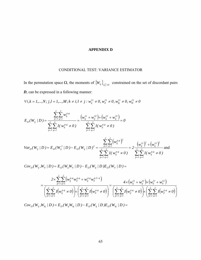
APPENDIX D
CONDITIONAL TEST: VARIANCE ESTIMATOR
In the permutation space Ω, the moments of 0wij 11
ijW
≠ constrained on the set of discordant pairs
D, can be expressed in a following manner:
0w,0w,0w,0w:jl;ik;M,...,1l,j;N,...,1k,i 11kl
11kj
11il
11ij ≠≠≠≠≠≠==∀
( ) ( )0
)0w(I
wwww
)0w(I
w)D|W(E 2
1p
2
1q
q,pij
21ij
12ij
22ij
11ij
2
1p
2
1q
q,pij
2
1p
2
1q
q,pij
ij =≠
+++=
≠=
∑∑∑∑
∑∑
= == =
= =Ω
( ) ( ) ( )∑∑∑∑
∑∑
= == =
= =
≠
+=
≠=−= 2
1p
2
1q
q,pij
212ij
211ij
2
1p
2
1q
q,pij
2
1p
2
1q
2q,pij
2ij
2ijij
)0w(I
ww2
)0w(I
w)D|W(E)D|W(E)D|W(Var ΩΩΩ and
=−= )D|W(E)D|W(E)D|WW(E)D|W,W(Cov ilijilijilij ΩΩΩΩ
( )
( ) ( )( ) ( )
( ) ( )⎟⎟⎠
⎞⎜⎜⎝
⎛≠×⎟⎟
⎠
⎞⎜⎜⎝
⎛≠
+×+×=
⎟⎟⎠
⎞⎜⎜⎝
⎛≠×⎟⎟
⎠
⎞⎜⎜⎝
⎛≠
+×=
∑∑∑∑∑∑∑∑
∑∑
= == == == =
= =
−
2
1p
2
1q
q,pil
2
1p
2
1q
q,pij
12il
11il
12ij
11ij
2
1p
2
1q
q,pil
2
1p
2
1q
q,pij
2
1p
2
1q
q3,pil
q,pij
q,pil
q,pij
0wI0wI
wwww4
0wI0wI
wwww2
=−= )D|W(E)D|W(E)D|WW(E)D|W,W(Cov kjijkjijkjij ΩΩΩΩ
65

( )
( ) ( )( ) ( )
( ) ( )⎟⎟⎠
⎞⎜⎜⎝
⎛≠×⎟⎟
⎠
⎞⎜⎜⎝
⎛≠
+×+×=
⎟⎟⎠
⎞⎜⎜⎝
⎛≠×⎟⎟
⎠
⎞⎜⎜⎝
⎛≠
+×=
∑∑∑∑∑∑∑∑
∑∑
= == == == =
= =
−
2
1p
2
1q
q,pkj
2
1p
2
1q
q,pij
21kj
11kj
21ij
11ij
2
1p
2
1q
q,pkj
2
1p
2
1q
q,pij
2
1p
2
1q
q,p3kj
q,pij
q,pkj
q,pij
0wI0wI
wwww4
0wI0wI
wwww2
0)D|W,W(Cov klij =Ω .
The moments of the W follow:
( ) 0D|WE)D|W(E0w:j,i
ij11ij
== ∑≠
Ω
=⎟⎟⎟
⎠
⎞
⎜⎜⎜
⎝
⎛
= ∑≠
DWVar)D|W(Var
0w:j,i
ij
11ij
ΩΩ
( ) ( ) (∑∑∑≠≠
≠≠≠
≠≠
++=
0wand0w:ik,j,i
kjij
0wand0w:jl,j,i
ilij
0w:j,i
ij
11kj
11ij
11il
11ij
11ij
D|W,WCovD|W,WCovD|WVar ΩΩΩ ) .
In the above equations I(x) designates the indicator function.
66
BIBLIOGRAPHY
1. Zhou XH, Obuchowski NA, McClish DK. Statistical Methods in Diagnostic Medicine. Wiley & Sons Inc.: New York, 2002.
2. Swets JA, Picket RM. Evaluation of Diagnostic Systems: Methods from Signal Detection Theory. Academic Press: New York, 1982.
3. Greenhouse SW, Mantel N. The evaluation of diagnostic tests. Biometrics 1950; 6(4): 399-412.
4. Metz CE. Basic Principles of ROC analysis. Seminars in Nuclear Medicine 1978; 8(4): 283-298.
5. Metz CE. ROC methodology in radiologic imaging. Investigative Radiology 1986; 21(9): 720-733.
6. Campbell G. Advances in statistical methodology for the evaluation of diagnostic and laboratory tests. Statistics in Medicine 1994; 13: 499-508.
7. Lee WC, Hsiao CK. Alternative summary indices for the receiver operating characteristic curve. Epidemiology 1996; 7: 605-611.
8. Hilden J. The area under the ROC curve and its competitors. Medical Decision Making 1991; 11: 95-101.
9. Hanley JA. The Robustness of the ‘Binormal’ Assumption Used in Fitting ROC Curves. Medical Decision Making 1988; 8(3): 197-203.
10. Dorfman DD, Alf JrE. Maximum likelihood estimation of parameters of signal detection theory and determination of confidence intervals – rating-method data. Journal of Mathematical Psychology 1969; 6: 487-496.
11. Metz CE, Herman BA, Shen J. Maximum likelihood estimation of receiver operating characteristic (ROC) curves from continuously distributed data. Statistics in Medicine 1998; 17: 1033-1053.
12. Zou KH, Hall WJ, Shapiro DE. Smooth nonparametric receiver operating characteristics (ROC) curves for continuous diagnostic tests. Statistics in Medicine 1997; 16(9): 2143-2156.
13. Hanley JA, McNeil BJ. The meaning and use of the Area under Receiver Operating Characteristic (ROC) Curve. Radiology 1982; 143: 29-36.
14. Faraggi D, Reiser B. Estimation of the area under the ROC curve. Statistics in Medicine 2002; 21: 3093-3106.
67

15. Noether GE. Elements of Nonparametric Statistics. Wiley & Sons Inc.: New York 1967.
16. Bamber D. The area above the ordinal dominance graph and the area below the receiver operating characteristic graph. Journal of Mathematical Psychology 1975; 12: 387-415.
17. Hanley JA, McNeil BJ. A method of comparing the area under two ROC curves derived from the same cases. Radiology 1983; 148: 839-843.
18. Wieand HS, Gail MM, Hanley JA. A nonparametric procedure for comparing diagnostic tests with paired or unpaired data. I.M.S. Bulletin 1983; 12: 213-214.
19. DeLong ER, DeLong DM, Clarke-Pearson DL. Comparing the Area under Two or More Correlated Receiver Operating Characteristic Curves: A Nonparametric Approach. Biometrics 1988; 44(3): 837-845.
20. Wieand HS, Gail M, James B, James K. A family of nonparametric statistics for comparing diagnostic markers with paired or unpaired data. Biometrika 1989; 76: 585-592.
21. Metz CE, Wang P-L, Kronman HB. A new approach for testing the significance of differences between ROC curves measured from correlated data. Information Processing in Medical Imaging VIII, F. Deconick (ed.) 1984; 432-445. The Hangue: Martinus Nijhof.
22. Arvesen JN. Jackknifing U-statistics. Annals of Mathematical Statistics 1969; 40(6): 2076-2100.
23 Beam CA, Wieand SH. A statistical method for the comparison of a discrete diagnostic test with several continuous diagnostic tests. Biometrics 1991; 47(3): 907-919.
24. Venkatraman ES, Begg CB. A distribution-free procedure for comparing receiver operating characteristic curves from a paired experiment. Biometrika 1996; 83(4): 835-848.
25. Venkatraman ES. A permutation test to compare receiver operating characteristic curves. Biometrics 2000; 56: 1134-1136.
26. Hoeffding W. A class of statistics with asymptotically normal distribution. Annals of Mathematical Statistics 1948; 19(3): 293-325.
27. Rockette HE, Campbell WL, Britton CA, Holbert JM, King JL, Gur D. Empiric assessment of parameters that affect the design of multireader receiver operating characteristic studies. Academic Radiology 1999; 6: 723-729.
28. Zhang DD, Zhou XH, Freeman DH, Freeman JL. A nonparametric method for the comparison of partial areas under ROC curves and its application to large health case data sets. Statistics in Medicine 2002; 21: 701-715.
29. Zhou XH, Gatsonis CA. A simple method for comparing correlated ROC curves using incomplete data. Statistics in Medicine 1996; 15: 1687-1693.
30. Metz C., Herman BA, Roe CA. Statistical comparison of two ROC estimates obtained from partially paired datasets. Medical Decision Making 1998; 18: 110-121.
31. Bandos AI, Rockette HE, Gur D. Small sample size properties of the nonparametric comparison of the area under two ROC curves. Medical Image Perception Society Conference X, September 2003, Durham, NC.
68

32. Bandos AI, Rockette HE, Gur D. A permutation test sensitive to differences in areas for comparing ROC curves from a paired design. Statistics in Medicine 2005; scheduled for 24(19).
33. Bandos AI, Rockette HE, Gur D. A conditional nonparametric test for comparing areas under two ROC curves from a paired design. Academic Radiology 2005; 12: 291-297.
34 Obuchowski NA, Rockette HE. Hypothesis testing of diagnostic accuracy for multiple readers and multiple tests an ANOVA approach with dependent observations. Communications in Statistics: Simulation and Computation 1995; 24(2): 285-308.
35. Dorfman DD, Berbaum KS, Metz CE. Receiver operating characteristic rating analysis: Generalization to the population of readers and patients with the jackknife method. Investigative Radiology 1992; 27: 723-731.
36. Roe CA, Metz CE. Variance-components modeling in the analysis of receiver operating characteristic index estimates. Academic Radiology 1997; 4: 587-600.
37. Beiden SV, Wagner RF, Campbell G. Components-of-variance models and multiple-bootstrap experiments: An alternative method for random-effects receiver operating characteristic analysis. Academic Radiology 2000; 7: 341-349.
38. Song HH. Analysis of correlated ROC areas in diagnostic testing. Biometrics 1997: 53(1): 370-382.
39. Obuchowski NA, Lieber ML. Confidence intervals for the receiver operating characteristic area in studies with small samples. Academic Radiology 1998; 5: 561-571.
40. Hajian-Tilaki KO, Hanley JA. Comparison of three methods for estimating the standard error of the area under the curve in ROC analysis of quantitative data. Academic Radiology 2002; 9: 1278-1285.
41. Efron B, Tibshirani RJ. An introduction to the bootstrap. Chapman & Hall: New York, NY, 1993.
42. Efron B. Bootstrap Methods: Another look at the jackknife. The Annals of Statistics 1979; 7: 1-26.
43. Mossman D. Resampling techniques in the analysis of non-binormal ROC data. Medical decision making 1995; 15: 358-366.
44. McNemar Q. Note on the sampling error of the differences between correlated proportions or percentages. Psychometrika 1947; 12: 153-157.
45. Bunch PC, Hamilton JF, Sanderson GK, Simmons AH. A fee-response approach to the measurement and characterization of radiographic-observer performance. Journal of Applied Photography and Engineering 1978; 4: 166-171.
46. Chakraborty DP. Maximum-likelihood analysis of free-response receiver operating characteristic (FROC) data. Medical Physics 1989; 16: 561-568
47. Chakraborty DP, Winter LHL. Free-response methodology: Alternative analysis and a new observer-performance experiment. Radiology 1990; 174: 873-881.
69