nonlinear system representation...schetzen, the volterra and wiener theories of nonlinear systems,...
TRANSCRIPT

1
NONLINEAR SYSTEM REPRESENTATION
Tommy W. S. Chow, City University of Hong Kong Hong-Zhou Tan, University of Manitoba Yong Fang, Shanghai University J. Webster (ed.), Wiley Encyclopedia of Electrical and Electronics Engineering Online Copyright © 2001 by John Wiley & Sons, Inc. All rights reserved. Article Online Posting Date: December 20, 2001
CONTENTS
• TOP OF ARTICLE • INPUT-OUTPUT SYSTEM REPRESENTATION • NONLINEAR DIFFERENTIAL ALGEBRAIC REPRESENTATION • VOLTERRA REPRESENTATION • STATE-SPACE REPRESENTATION • BILINEAR REPRESENTATION • NARMA REPRESENTATION • FUZZY-LOGIC NONLINEAR REPRESENTATION • NONLINEAR REPRESENTATION USING NEURAL NETWORKS • MODEL-FREE REPRESENTATION • FEATURES OF NONLINEAR REPRESENTATIONS • EXAMPLE • CONCLUDING REMARKS • ACKNOWLEDGMENT
BIBLIOGRAPHY 1. D. E. Thompson, Design Analysis: Mathematical Modeling of Nonlinear Systems, New York: Cambridge
Univ. Press, 1999. 2. M. Vidyasagar, Nonlinear Systems Analysis, 2nd ed., Englewood Cliffs, NJ: Prentice-Hall, 1993. 3. A. J. Fossard, D. Normand-Cyrot, Nonlinear Systems, Modeling and Estimation, London: Chapman &
Hall, 1995. 4. M. Schetzen, The Volterra and Wiener Theories of Nonlinear Systems, New York: Wiley, 1980. 5. J. L. Casti, Nonlinear System Theory, Orlando, FL: Academic Press, 1985. 6. P. G. Drazin, Nonlinear Systems, New York: Cambridge Univ. Press, 1992. 7. J. S. Bendat, A. G. Piersol, Engineering Applications of Correlation and Spectral Analysis, New York:

2
Wiley, 1993. 8. R. R. Mohler, Bilinear Control Processes, New York: Academic Press, 1973. 9. P. N. Paraskevopoulos, A. S. Tsirikos, K. G. Arvanitis, A new orthogonal series approach to state space
analysis of bilinear systems, IEEE Trans. Automat. Control, 39: 793-797, 1994. 10. S. Chen, S. A. Billings, Representation of nonlinear systems: the NARMA model, Int. J. Control, 49(3):
1013-1032, 1989. 11. I. J. Leontaritis, S. A. Billings, Input-output parametric models for non-linear systems, part I:
deterministic non-linear systems, Int. J. Control, 41(2): 303-328, 1985. 12. E. D. Sontag, Realization theory of discrete-time nonlinear systems: Part I - the bounded case, IEEE
Trans. Circuits Syst. 26: 342-356, 1979. 13. L. Zadeh, Fuzzy sets, Inf. Control, 8: 338-353. 14. C. C. Lee, Fuzzy logic in control systems: fuzzy logic controller, part I, IEEE Trans. Syst. Man Cybern.,
SMC-20: 404-418, 1990. 15. C. C. Lee, Fuzzy logic in control systems: fuzzy logic controller, part II, IEEE Trans. Syst. Man Cybern.,
SMC-20: 419-435, 1990. 16. T. Takagi, M. Sugeno, Fuzzy identification of systems and its applications to modeling and control, IEEE
Trans. Syst. Man Cybern., 15: 116-132, 1985. 17. E. H. Mamdani, Applications of fuzzy algorithms for simple dynamic plant, Proc. IEE, 121(12): 1585-
1588, 1974. 18. C. J. Harris, C. G. Moore, M. Brown, Intelligent Control: Some Aspects of Fuzzy Logic and Neural
Networks, London and Singapore: World Scientific Press, 1993. 19. B. H. Wang, G. Vachtsevanos, Learning fuzzy logic control: an indirect control approach, Proc. IEEE
Int. Conf. on Fuzzy Systems, San Diego, CA, 1992, pp. 297-304. 20. T. J. Ross, Fuzzy Logic with Engineering Applications, New York: McGraw-Hill, 1995, Chapter 13. 22. J. Y. Li, T. W. S. Chow, Functional approximation of higher-order neural networks, J. Intell. Syst., 6(3-
4): 239-260, 1996. 23. J. J. Hopfield, Learning algorithm and probability distributions in feed-forward and feed-back networks,
Proc. Nat. Acad. Sci. U.S.A., 84, 8429-8433, 1987. 24. K. Hornik, M. Stinchcombe, H. White, Multilayer feedforward networks are universal Approximators,
Neural Netw., 2: 359-366, 1989. 25. H.-Z. Tan, T. W. S. Chow, Blind identification of quadratic nonlinear models using neural networks with
higher-order cumulants, IEEE Trans. Ind. Electron., 47: 687-696 2000. 26. J. Y. F. Yam, T. W. S. Chow, A weight initialization method for improving training speed in feedforward
neural network, Neurocomputing, 30(1-4): 219-232, 1999. 27. J. Y. F. Yam, T. W. S. Chow, C. T. Leung, A new method in determining initial weights of feedforward
neural networks for training enhancement, Neurocomputing, 16(1): 23-32, 1997. 28. J. J. Hopfield, Neural networks and physical systems with emergent collective properties, Proc. Nat.
Acad. Sci. U.S.A., 79: 2554-2558, 1982. 29. C. L. Nikias, A. P. Petropuop, Higher-Order Spectra Analysis: A Non-linear Signal Processing
Framework, Englewood Cliffs, NJ: Prentice-Hall, 1993. 30. L. Ljung, System Identification: Theory for the User, 2nd ed., Upper Saddle River, NJ: Prentice-Hall,
1999. 31. G. A. Glentis, P. Koukoulas, N. Kalouptsidis, Efficient algorithm for Volterra system identification,

3
IEEE Trans. Signal Process., 47: 3042-3057, 1999. 32. A. U. Levin, K. S. Narendra, Recursive identification using feedforward neural networks, Int. J. Control,
61(3): 533-547, 1995. 33. L. X. Wang, J. M. Mendel, Fuzzy basis function, universal approximation, and orthogonal least squares
learning, IEEE Trans. Neural Netw., 3: 807-814, 1992. 34. H.-Z. Tan, Y. Fang, T. W. S. Chow, Wiener models identification based on the higher-order cumulants
and orthogonal wavelet neural networks, Int. J. Knowledge Based Intell. Eng. Syst., 3(2): 102-107, 1999. 35. T. W. S. Chow, C. T Leung, A non-linear autoregressive intergrated neural network model for short-term
load forecasting, IEE Proc. Gener. Transm. Distrib., 143(5): 500-506, 1996. READING LIST G. Anger, Inverse Problems in Differential Equations, New York: Plenum, 1990. B. Igelnik, Y.-H. Pao, Stochastic choice of basis functions in adaptive function approximation and the functional-link net, IEEE Trans. Neural Netw., 6: 1320-1329, 1995. W. J. Rough, An extended linearization approach to nonlinear system inversion, IEEE Trans. Automat. Control, AC-31(8): 725-733, 1986. S. N. Singh, A modified algorithm for invertibility in nonlinear systems, IEEE Trans. Automat. Control, 26: 595-598, 1981.
[EEEE Home] [A to Z] [Subjects] [Search]
Copyright ©1999-2000 by John Wiley & Sons, Inc. All rights reserved.

4
It has been said that whereas linearity is a specification of a field of activity, nonlinearity is a “nonspecification and its field is unbounded. In nature, nonlinearity is the rule rather than the exception, while linearity is a simplification adopted for analysis. Most practical systems used for control are essentially nonlinear, and in many applications, particular in the area of chaos, it is the nonlinear rather than the linear characteristics that are most used. Signals found in the physical world are also far from conforming to linear models. Indeed, the complex structure of dynamic systems makes it almost impossible to use linear models to represent them accurately. Nonlinear models are designed to provide a better mathematical way to characterize the inherent nonlinearity in real dynamic systems, although we may not be able to take all their physical properties into account. In this article, we will focus on other nonlinear techniques than modeling, which may provide readers with useful perspectives.
For most real-world practical applications, there are advantages to using nonlinear models to characterize the nonlinear relationships. Mathematical models may be expressed in the form of difference or differential equations. Depending on the given engineering problem and the circumstances, one mathematical model may be better suited than another. Figure 1 shows a typical system for processing and evaluating a system model. In general, nonlinear representations can be classified into three types: (1) system input-output representation, (2) state-space representation, and (3) model-free representation. The first type considers the input-output behavior of a system without considering any internal variations. The second type focuses on both internal and external performance of the system, and the last type focuses on the representation of nonlinear systems that cannot be handled by the other two approaches. Although the selection of the type of model is often quite subjective, it is usually the result of a compromise between the model selection and familiarity with the model itself. In this regard, a number of nonlinear techniques will be briefed in this article.
[EEEE Home] [A to Z] [Subjects] [Search]
Copyright ©1999-2000 by John Wiley & Sons, Inc. All rights reserved.
5
INPUT-OUTPUT SYSTEM REPRESENTATION Nonlinear system representation means the characterization of nonlinear systems using nonlinear mathematical models. In fact, nonlinear models may be considered as a tool for explaining the nonlinear behavior patterns in terms of a set of easily understood elements. Figure 2 shows the input-output representation approach for describing a given nonlinear system
where y(t) refers to the system output, u(t) refers to the system input, the independent variable t is time, and the f denotes a mathematical relationship describing the nonlinear behavior: the system yields the output y(t) when the system has a input u(t). Generally, the nonlinear mapping f is very complicated, and there is no single technique suitable for the analysis of all nonlinear behaviors. In order to appreciate the complexity associated with nonlinear systems, it is best first to review the relative simplicity associated with linear systems. The main reason is that dynamic system analysis relies heavily on linear models, due to their comprehensiveness and the availability of well-developed linear system theories.
A system (1) is called a linear system if it satisfies
We note two important features. One is that the sum of inputs results in the sum of the responses to the individual inputs, and the other is that a multiple of an input results in the same multiple of the corresponding output. An electric circuit containing a capacitor and a resistor is a common example used for explication. In this article we will mainly focus on the theoretical aspect.
A dynamic system is called anticipatory or noncausal if its outputs depend on the past, present, and future values of its inputs. A system is called nonanticipatory or causal if its outputs depend only on the past and present values of its inputs. We say that a system is time-invariant if its properties are invariant to a shift of time.
First let us consider the following linear system, which can be described as single-input, single-output, time-invariant, and causal (1):

6
where h(t) is called the impulse response of the system. Without loss of generality, this system can be assumed to satisfy the following assumptions: (1) h(t) is a real-valued function defined for t (- , ) and piecewise continuous except possibly at t = 0; (2) the input signal is a real-valued function defined for t (-, ) and piecewise continuous. These conditions imply that the output signal is a continuous, real-valued function defined for t (- , ). In practical engineering, however, it is often assumed that h(t) is a real-valued function defined for t (0, ), corresponding to causality. Considering only input signals that are zero prior to t = 0, which allows the upper limit in Eq. (3) to be replaced by t, a change of the integration variable shows that Eq. (3) can be rewritten as
In this form the one-sidedness assumption on h(t) implies that the upper limit can be lowered to t, while a one-sided assumption on u(t) enables the lower limit to be raised to 0. The representation (3) is usually favored for time-invariant systems.
If the assumption that the system is time-invariant is dropped, the following input-output representation applies. We replace h(t) with a real-valued function h(t, s) defined for t (- , ), s (- , ), with h(t, s) = 0 if s > t, that is,
It is straightforward to confirm that this represents a linear system in a general sense. In fact, the assumption on h(t, s) implies causality; only the delay-invariance property has been dropped. Typically h(t, s) is allowed to contain impulses for s = t, but otherwise is piecewise continuous for t s 0. The range of integration in Eq. (5) can be narrowed as discussed before.
Comparison of Eqs. (4) and (5) highlights the fact that time-invariant linear systems are, in fact, special cases of time-varying linear systems. Thus, the impulse function h(t, s) in (5) is called time-invariant if there exists an impulse response h (t) such that
An easy way to check for time invariance of h(t, s) is to check the condition h(0, s - t) = h(t, s). If this is satisfied, then setting h (t) = h(0, - t) verifies Eq. (6).
[EEEE Home] [A to Z] [Subjects] [Search]
Copyright ©1999-2000 by John Wiley & Sons, Inc. All rights reserved.

7
NONLINEAR DIFFERENTIAL ALGEBRAIC REPRESENTATION The specification of the modeling problem for a linear system is simplified by the fact that it is easy to parametrize the response via a defined coordinate system. This fact enables us to reduce the problem of constructing a standard model from an input-output relation to a linear-algebra expression. In the nonlinear case, there is no such global coordinate system. Usually we have to be cautious in defining what we mean by the problem data. We cannot simply assume the system response to be as simple as an infinite sequence of functions or an impulse function.
The first step in constructing a nonlinear model is the development of a differential representation for describing the system input-output behavior. Clearly, there are a number of ways in writing differential equations that describe the behavior of different dynamic systems. No single one of them is preferable in all circumstances. In general, the result required and the familiarity of the investigator with a particular method determine the form of the differential equations.
One particularly convenient method of characterizing the behavior of a nonlinear system is by (2)
where u(t) is the system input, y(t) is the system output, and f(·) is an arbitrary nonlinear function. Figure 3 shows the corresponding input-output relationship. There are several reasons for the importance of this differential algebraic form of the system equations. Apart from the notational simplicity, one can deal with all systems by means of a compact notation instead of having to write a system of simultaneous differential equations. Also, this representation is the one that most modern literature in the theory of differential equations makes use of.
It is natural to represent the output in terms of the input as a series expansion
where the real-valued function of n variables hi(t1,t2, ,tn), i = 0, 1, 2, , is equal to zero if any ti < 0, that is to say, the system is causal. Obviously the system is not linear, and it is a time-invariant system if hi(t1,t2,,tn) = h i(t1 - t2 - - tn). Formally the expansion (8) is a generalization of the linear-variation-of-constants formula (5). Clearly, this type of modeling problem for nonlinear systems may be expressed as follows: given a sequence of input-output pairs, find a canonical model (8) whose input-output behavior generates the series of impulse functions hi, i = 0, 1, 2, .

8
The modeling process is rather straightforward if there are no further hypotheses on the analytic behavior of f in Eq. (7) and there is a suitable definition of the canonical model. In general the problem is unsolvable, but the following theorem (3) provides conditions under which the expansion (8) exists and is unique.
Theorem 1 If the nonlinear relationship f in Eq. (7) is an analytic vector field and Eq. (7) has a solution on [0, T] with y(0) = h0(0), then the input-output behavior of Eq. (7) has a unique representation expressed by Eq. (8) on [0, T] (3).
Now it is quite clear that the condition of analyticity of the defining vector field is essential. The reason is clear: analyticity forces a certain type of rigidity upon the system, namely, the system behavior is determined by its response in an arbitrarily small open set. Fortunately, it is a property possessed by all systems defined by sets of algebraic equations.
[EEEE Home] [A to Z] [Subjects] [Search]
Copyright ©1999-2000 by John Wiley & Sons, Inc. All rights reserved.

9
VOLTERRA REPRESENTATION In this section, we introduce a special type of nonlinear series, Volterra series, which exhibit many important features for nonlinear system modeling, control, and signal processing. Put in simple words, a Volterra series contains symmetrical parameters, Volterra kernels, of order n, which are nth-order impulse responses, to represent nonlinear dynamics. In most cases, we have to estimate the Volterra kernels. This is usually a computationally rather complex procedure and is best performed offline.
Based on a real-valued function of n variables hn(t1, t2, , tn) defined for ti (- , ), i = 1, 2, , n, and such that hn(t1,t2, ,tn) = 0 if any ti < 0, we consider the following system response:
Equation (9) is a nonlinear model of degree n, in which application of the input au(t), where a is a scalar, yields the output an y(t). The impulse function hn(t1, t2, ,tn) is called the model kernel.
If the input signal is one-sided, then all the upper limits can be replaced by t. A change of each variable of integration shows that Eq. (9) can be rewritten in the following form:
In most science and engineering applications the above model is usually obtained from physical systems that are structured in terms of interconnections of linear subsystems and simple nonlinearity, especially time-invariant linear subsystems and nonlinearities that can be represented in terms of multipliers. Simply by tracing the input signal through the system structure, it is easy to derive the system kernels from the subsystem kernels for the interconnection-structured systems. The model (10) can also arise with a state-equation description of a nonlinear system, which will be discussed in detail later on.
A model described by a finite sum of terms like those in Eq. (10),

10
is called an Nth-order Volterra model (4). It is worth noting that, as special cases, static nonlinear models described by a polynomial or power series in the input,
or
are included in this Volterra model simply taking hn(t1, t2, , ti) = ai (t1) (t2) (ti).
As a Volterra series is an infinite series, convergence conditions must be considered. Usually these conditions include a bound on the time interval and a bound for u(t) on this interval, but the determination of the bound is often difficult.
With reference to the derivation of the Volterra representation for a nonlinear model, it is reasonable to consider the output y(t) of a nonlinear model at a particular time t as depending on all values of the input at times prior to t, which implies that y(t) depends on u(t - i) for all i 0. In other words, the present output depends on all past input values. This viewpoint leads to the following idea. If u(t - i) for all i 0 can be described by a set of quantities u1(t), u2(t), , then the output y(t) can be represented as a nonlinear function of these quantities,
Suppose that t is fixed, and the input u(t - i) is an element of the Hilbert space L2(0, ) of square-integrable functions, that is,
Also, suppose that w1(t), w2(t), is an orthonormal basis for this space:
The value of the inputs at any time of the past is in the form

11
where
Equation (17) yields a characterization of the past of u(t) in terms of u1(t), u2(t), , regardless of t. Expand the function f(u1(t), u2(t), ) into a power series, so that the output at any time t is
Substituting Eq. (18) into Eq. (19), we obtain
In view of the definition of the kernel, this is the kind of representation that has been discussed.
The generalization of the Laplace transform to functions of variables is of importance for nonlinear system modeling (5). This representation is very handy for characterizing model properties and for describing the model input-output response. Given a time-invariant linear model, the transfer function of the model is the Laplace transform of h(t),
For one-sided input signals, by using the convolution property of the Laplace transform, the input-output response can be expressed as
or
where Y(s) and U(s) are the transforms of y(t) and u(t), respectively. If a model transfer function is given and the input signal of interest has a simple transform U(s), then the utility of this representation for computing
12
the corresponding output signal is quite clear. Moreover, many system properties can be expressed rather simply as properties of H(s). Consider that an nth-order nonlinear model with one-sided inputs is represented by
Because of the properties of the multivariable Laplace transform, there is no direct way of updating in a form similar to Eq. (23). An indirect approach is therefore employed, writing Eq. (24) as the following pair of equations:
Then, Eq. (25) can be written as a relationship between Laplace transforms in the form
Now let us look at the Laplace transform representation of Volterra models. It basically involves the collection of submodel transfer functions in Eq. (25). Obviously, response calculations are performed by summing the responses of the submodels as calculated individually by association of variables:
This summation requires consideration of the convergence properties of an infinite series of time functions. Usually convergence is crucially dependent on properties of the input signals, for example, bounds on their amplitude. Using the growing exponential signals as inputs of Volterra models, it is easy to determine the transfer function of the model.
The nonlinear Volterra models discussed above can be developed for discrete-time cases. There are differences, of course, but these mostly are differences in technical details or interpretation of the results. The situation is similar to the linear case, where the continuous- and discrete-time theories look much the same.
Consider the following discrete-time system representation:

13
The input signal u(t) and the output signal y(t) are real sequences that are assumed to be zero for t < 0. The kernel h(i0, i1, , il) is real, and assumed to be zero for any i0, i1, , il < 0. It is straightforward to verify that a system described by Eq. (29) is nth-order, time-invariant, and causal. It is noted that the upper limits on the summations can be lowered to t. Since, for any t, y(t) is given by a finite summation, problems like continuity and integrability in the continuous-time case do not arise with regard to the representation in Eq. (29). Notice that direct transmission terms are explicitly displayed in Eq. (29), and there is no need to consider impulsive kernels. The familiar sum-over-permutations argument shows that the kernel in Eq. (29) can be replaced by the symmetric kernel hsym(i0, i1, , in) = 1/n! (·) h(i (1), i (2), , i (n)) without loss of generality. From the symmetric kernel representation, a triangular-type kernel can be defined as htri(i0, i1, , il) = hsym(i0, i1, , il) (i1 - i2, i2 - i3, , il-1 - il) (6), where the special multivariable step function takes the form
It is easy to verify that when n = 2, this setup yields consistent results in going from the symmetric kernel to the triangular kernel and vice versa. The higher-degree cases are less easy but still straightforward.
The regular kernel representation is another special form of the system kernel. With the triangular kernel representation
a simple change of variables argument gives
where

14
Also it is noticed that the upper limits of the summation in Eqs. (31) and (32) can be replaced by finite quantities.
Although only time-invariant systems are usually considered, a general representation of the form
is also very important. It is natural to follow the continuous-time case and call a kernel h(t, i0, i1, , il) time-invariant if h(0, i0 - t, i1 - t, , il - t) = h(t, i0, i1, , il). If this relationship holds, then setting g(i0, i1, , il) = h(0, - i0, - i1, , - il) yields the representation
which is equivalent to Eq. (34). Actually the above equation can be described as
which is in the same form as Eq. (29).
With these basic representations, the description of Volterra models is simply a matter of finite sums of the terms in Eq. (29). In circuit theory, signal processing, and communication applications, the following two truncated Volterra models are usually utilized:
Quadratic Model:
Cubic Model:

15
Of course the convergence issue is important for Volterra models, but the basic approach to convergence in the continuous-time case carries over directly (4). In the frequency domain, the z-transform representation is used for Volterra systems in just the same way that the Laplace transform is used in the continuous-time case (7). A transfer function for a nth-order discrete-time system [Eq. (29)] is defined as the z-transform of a kernel for the system. That is,
Unfortunately, it seems to be impossible to represent the input-output relationship in Eq. (29) directly in terms of U(z), Y(z), and H(z1, z2, , zl). The usual alternative is to rewrite Eq. (29) as a pair of equations
Then the first equation has the form
while the second equation is an association of variables that involves contour integrations of the following form:
As far as the regular transfer function is concerned, the formulas in Eqs. (40) and (41) do not directly apply. However, by suitably restricting the class of input signals, a much more explicit formula can be obtained. By establishing a basic expression for the z-transform of the input-output relation (32), the regular transfer function is cast in the following form:

16
where each Hi1i2 il-1 (zl) is defined according to
[EEEE Home] [A to Z] [Subjects] [Search]
Copyright ©1999-2000 by John Wiley & Sons, Inc. All rights reserved.

17
STATE-SPACE REPRESENTATION
A state-space representation is usually used for describing physical systems. If the state of a system is known, then any output or quantity of interest with respect to certain performance indices can be achieved. To determine the state of a system as a function of time, we need a set of equations to relate the inputs state of the system. One approach for obtaining that set of equations is to consider each state variable as an output, to be determined via an nth-order differential or difference equation. Using the state-space approach, we will be able to write n first-order differential or difference equations for the n state variables of the system. In general they will be coupled equations, that is, they will have to be solved simultaneously. For nonlinear systems, these first-order equations will be nonlinear ones. One advantage of the state-space representation is that once the first-order equations are solved, complete knowledge of the system behavior is obtained. All outputs are algebraic functions of the state variables. No further solution of a differential or difference equation is needed.
The input-output behavior of a nonlinear system can be characterized by first-order differential or difference equations
or
where x n are the internal states of the system, u m are the inputs, y q are the outputs and f : n+m n, g : n q. While the inputs and outputs of a system are generally the tangible physical data, it is
the state variables that assume the dominant role in this formulation. It is possible that quantities that are not of interest will lead to an unnecessarily complicated problem.
A major difficulty in dealing with nonlinear equations is that the existence and the uniqueness of solutions, even in a local sense, cannot be taken for granted. As a matter of fact, there does not exist any general methodology to determine the nonlinear relations f and g. Instead, various simplified nonlinear models are widely used in practical engineering applications. The so-called bilinear model is among these. We will discuss the bilinear representation in detail later.
Now let us look at the discrete-time nonlinear model (47). It is assumed that the initial state is x(0) = 0, and that f(0, 0) = 0 and g(0, 0) = 0. Then the functions f(x, u) and g(x, u) can be represented using a Taylor series

18
about x = u = 0 of order sufficient to permit calculating the polynomial input-output representation to the degree desired:
where x(i) = x x x (i factors) and Fij, Gij are the standard Kronecker products. Just as in the continuous-time case, the crucial requirement is that the kernels through order N corresponding to Eq. (48) should be identical to the kernels through order N corresponding to Eq. (47).
[EEEE Home] [A to Z] [Subjects] [Search]
Copyright ©1999-2000 by John Wiley & Sons, Inc. All rights reserved.

19
BILINEAR REPRESENTATION
In the class of nonlinear dynamic systems, bilinear models are probably the simplest ones. They take the form (8)
or
where F, Ni, and C are n × n real matrices and G, D are n × m real matrices. Bilinear models are widely used in control systems, signal processing, and communications, because they can be parametrized by matrix operations and lead to linear models of familiar type.
The solution of Eq. (49) for x(t) in terms of a series expansion is given by (9)
where Nx(t)u(t) = ( mi=1 Niui)x(t). The first term xl(t) in Eq. (51) is the solution, for the state vector x(t), of the
linear system described by the equation (t) = Fx(t) + Gu(t). The second term xb(t) is due to the bilinear term ( m
i=1 Niui)x(t) appearing in Eq. (49). The term xl(t) may be approximated via orthogonal series as follows:

20
where fr(t) = [f0(t), f1(t), , fr-1(t)]T is the orthogonal basis vector and
where e is a constant r × 1 vector, whose form depends on the particular orthogonal series; Pr is the r × r operational matrix of integration; and U is the m × r coefficient matrix of the input u(t), defined by
An approximation of Eq. (54) is obtained by keeping the first k power-series terms of eFt and eF(t-t1) appearing
in xl(t).
Similarly to xl(t) in Eq. (54), the second term xb(t) can be expressed by the following equations:
where
Then Eq. (51) can be replaced by an orthogonal expression in the form
This makes the study of controllability and observability of bilinear models much easier via orthogonal functions.
[EEEE Home] [A to Z] [Subjects] [Search]
Copyright ©1999-2000 by John Wiley & Sons, Inc. All rights reserved.

21
NARMA REPRESENTATION
In this section, the nonlinear autoregressive moving-average (NARMA) model is discussed. Detailed nonlinear system modeling using this model can found in Refs. (10) and (11).
Now let us consider the following discrete-time system:
where y(t) Y, the output set of dimension q; x(t + 1), x(t) X, the state set of dimension n; u(t) U, the input set of dimension m; t Z, the set of integers; f : Z × X × U X is the one-step-ahead state transition function; and g : Z × X × U Y is the output function. Assuming that the system is at the zero equilibrium point at time t = 1, the zero-state response for an input sequence of length t is given by
where ht : Ut Y. The function ht is a different function for every t = 1, 2, , because the domain of definition Ut is different. Assume that the response functions ht are continuously differentiable functions, and let the vector ut(t) = [u(t), u(t - 1), , u(1)]T; then
Let ytk(t) = [y(t), y(t - 1), , y(t + k - 1)]T and ut
k(t) = [u(t + k - 1), u(t + k - 2), , u(t)]T. Then Eq. (63) can be rewritten as
where yk(t) Yk, utk Uk, ut-1 Ut-1. The function Ht
k : Uk × Ut Yk can be defined for any k = 1, 2, , t = 1, 2, , when the response function ht is known for t = 1, 2, . The function Ht
k is continuously differentiable, since it is the Cartesian product of k response functions of continuously differentiable. For simplicity, we let z = ut+1
k Uk, x = ut Ut. The assumptions on the function Htk are the following:
Assumption 1 max[rank dHt
k(z,x)/dx]=n for any z = ukt+1 Uk, x = ut Ut and any t, k =1, 2, .

22
Assumption 2 rank dHt
k(0,0)/dx = n for some t and some k.
We can prove the following theorem.
Theorem 2 For any nonlinear system satisfying Assumptions 1 and 2, there exists a number l and a continuous function
: yl × ul y such that the recursive input-output representation given as
has the same input-output behavior as the original system in a restricted operating region and around the zero equilibrium point.
Recall the autoregressive moving-average (ARMA) model in the linear case,
The model (65) is called the NARMA model (10) by extension. The NARMA model can be further extended to a nonlinear stochastic system. Let the estimate (t) denote the prediction of y(t) that is in the form
The prediction error vector e(t) can be calculated as e(t) = y(t) - (t); it is a vector random variable and shows how much the actual output at time t differs from the predicted one. Then the stochastic NARMA model can be expressed as (12)
[EEEE Home] [A to Z] [Subjects] [Search]
Copyright ©1999-2000 by John Wiley & Sons, Inc. All rights reserved.

23
FUZZY-LOGIC NONLINEAR REPRESENTATION
The real physical world is very complex, so that problems may always arise from many uncertain factors. The uncertainty in all engineering problems motivates us to establish appropriate methods or models to express the uncertainty. Fuzzy logic is a mathematical approach developed by Zadeh (13) to tackle this issue. Because of their outstanding ability to relate fuzzy sets with humanistic variables, fuzzy-logic nonlinear models have recently been widely used in the areas of control, signal processing, and communication applications. They have demonstrated their versatility in representing complex nonlinear physical systems using linguistic rules of the IF-THEN form. For example, Fig. 4 shows the nonlinear relation between the probability of a machine fault and the vibration magnitude. The mapping shown in Fig. 4 can be best described by fuzzy logic.
A fuzzy-logic model consists of an identification algorithm that adjusts the parameters. The model is designed from certain IF-THEN rules using fuzzy-logic principles. In general, there are two strategies for combining numerical and linguistic information using adaptive fuzzy models. In the first, one uses linguistic information to construct an initial fuzzy-logic model. The parameters of that model are then adjusted in accordance with numerical information. The final fuzzy-logic model can then be obtained by combining numerical and linguistic information. In the second strategy, two separate fuzzy-logic models are initially constructed from numerical information and linguistic information. These models are then averaged to obtain the final fuzzy-logic model.
The most popular fuzzy logic models may be classified into three types: the pure fuzzy-logic model, Takagi and Sugeno's fuzzy model, and fuzzy-logic models with fuzzifier and defuzzifier (14, 15).
Pure Fuzzy-Logic Model Basically, this first type consists of a fuzzy rule base and a fuzzy inference engine. The rule base is a collection of fuzzy IF-THEN rules, and the inference engine is based on fuzzy-logic principles. The IF-THEN rules are to determine a mapping from fuzzy sets in the input universe to fuzzy sets in the output. They are of the following form:
where Fli and Gl are fuzzy sets, and u = [u1, u2, , un]T U and y V are input and output linguistic
variables, respectively. The major advantage of fuzzy logic is its remarkable ability to incorporate common sense, as reflected in decisions, into numerical information. Each fuzzy IF-THEN rule of Eq. (69) defines a fuzzy set Fl
1 × Fl2 × × Fl
n Gl in the product space U × V.
The most commonly used fuzzy-logic principle is the so-called sup-star composition. Let A be the input to the pure fuzzy-logic model. Then the output determined by each fuzzy IF-THEN rule of Eq. (69) is a fuzzy set A (R(l)) in V whose membership function is

24
where * is an operator such as minimization or multiplication, and A is the membership function of the fuzzy set A. The output of the pure fuzzy-logic system is a fuzzy set A (R(1), R(2), ,R(M)) in V that combines the M fuzzy sets in accordance with Eq. (70):
where the operator is maximization, that is, u y = u + y - uy. The model becomes a fuzzy dynamic model if there is feedback in the fuzzy-logic model. Takagi and Sugeno's Fuzzy Model The pure fuzzy-logic model constitutes the essential part of all fuzzy-logic models. By itself, however, it has the disadvantage that its inputs and outputs are fuzzy sets, whereas in most physical systems the inputs and outputs of a system are real-valued variables. In order to overcome this shortcoming, Takagi and Sugeno designed another fuzzy-logic model of which inputs and outputs are real-valued variables.
In this model (16), the following fuzzy IF-THEN rules are proposed:
where Fli are fuzzy sets, cl
i are real-valued parameters, yl is the model output due to the rule Ll, and l = 1, 2, , M. That is, they considered rules of which the IF part is fuzzy, but the THEN part is crisp. Also, the
output is a linear combination of input variables. For a real-valued input vector u = [u1, u2, , un]T, the output y(u) is a weighted average of the yl's:
where the weight wl represents the overall truth value of the premise of the rule Ll for input and can be determined by
where Fil is the member function of the fuzzy set Fi
l. The major advantage of this model lies in the fact that it provides a compact system equation (73). Hence, parameter estimation and order determination methods can be developed to estimate the parameters cl
i and the order M. A shortcoming of this model is, however, that the THEN part is not fuzzy, so that it cannot incorporate fuzzy rules from common sense and human decisions.

25
Fuzzy-Logic Models with Fuzzifier and Defuzzifier Models of this type (17) add a fuzzifier to the input and a defuzzifier to the output of the pure fuzzy-logic model. The fuzzifier maps crisp points in U to fuzzy sets in U, while the defuzzifier maps fuzzy sets in V to crisp points in V. The fuzzy rule base and fuzzy inference engine are the same as those described in the pure fuzzy-logic model.
Evidently the fuzzy-logic model with fuzzifier and defuzzifier has certain advantages over other nonlinear modeling techniques. First, it is suitable for engineering systems in that its input and outputs are real-valued variables. Second, it is capable of incorporating fuzzy IF-THEN rules from common sense and human decisions. Third, there is much freedom in the selection of fuzzifier, fuzzy inference engine, and defuzzifier, in order to obtain the most appropriate fuzzy-logic model for a given problem. Finally, we are able to design different identification algorithms for this fuzzy-logic model, so as to integrate given numerical and human information.
The fuzzifier that performs the mapping from a crisp point into a fuzzy set A in U can be a singleton or a nonsingleton fuzzifier. Singleton fuzzifiers have mainly been used, but nonsingleton fuzzifiers can be useful when the inputs are noise-corrupted.
There are at least three possible choices for the defuzzifer that performs a mapping from fuzzy sets in V into a crisp point y V:
1.The maximum defuzzifier, defined as
where B is a fuzzy set with support y. 2.The center average defuzzifier, defined as
where yl is the center of the fuzzy set Gl, that is, the point in V at which Gl(y) achieves its maximum value.
3.The modified center average defuzzifier, which is given as
where l is a parameter characterizing the shape of Gl (y) such that the narrower the shape of G
l (y), the smaller is l. For example, if G (y) = exp[-(y - yl)/ l]2, then l is such a parameter.
Fuzzy Control Summarized For nonlinear system modeling, fuzzy logic can be viewed as a versatile tool to perform nonlinear mapping. But in such an input-output nonlinear system model, the input signals should be representative and

26
sufficiently rich. In most cases, the fuzzy nonlinear model is based on inputs such as the rate of change of error, and the fuzzy model may be in continuous time or discrete time.
Figure 5 shows a typical fuzzy control system, in which input values are normalized and fuzzified, the fuzzy-model rule base is the control rule base used to produce a fuzzy region, and a defuzzification process is used to find the expected output value. A typical fuzzy learning control-system design is that proposed in 1993 by Harris et al. (18). Wang and Vachtsevanos (19) detailed an indirect fuzzy-control approach in 1992. In their early research, a separate fuzzy model was developed. A well-designed procedure was then used to calculate the control signal. More detailed discussion of control of nonlinear systems using fuzzy logic can be found in Refs. 18-20.
[EEEE Home] [A to Z] [Subjects] [Search]
Copyright ©1999-2000 by John Wiley & Sons, Inc. All rights reserved.

27
NONLINEAR REPRESENTATION USING NEURAL NETWORKS
Conventional model-based theoretical methods have dominated nonlinear-representation research over the last few decades. These methods depend on a mathematical characterization of the monitored system. The main disadvantage of such approaches is that they are very sensitive to the selection of model type, modeling errors, parameter variations, and measurement noise. The success of model-based representation approaches is heavily dependent upon the quality of the models as well. For most practical nonlinear physical systems, it is often very difficult, if not impossible, to describe them by sufficiently simplified analytical models. In view of these, there is great interest in developing a robust and less model-dependent methodology for representing a complex nonlinear dynamic system. To avoid the difficulties experienced in the classical nonlinear system modeling, neural-network-based nonlinear system modeling methods appeared to be an appealing alternative. The rationale behind this approach lies in the fact that a multilayer neural network (Fig. 6) with an appropriate nonlinear activation function can approximate any nonlinear relationship.
In using neural networks for nonlinear system modeling, their nonlinear functional approximation capability can be enhanced by using higher-order architectures. In Refs. (33) and (34) strong theoretical arguments were introduced for the functional-approximation capability of the random-vector version of functional-link nets (RVFL). (See Fig. 7.) The distinctive aspects of this network are that the parameters of the hidden layer, such as the weights and the thresholds, are selected randomly and independently in advance. The parameters of the output layer are learned using simple quadratic optimization, whereas under conventional approaches all parameters need to be learned using complicated nonquadratic optimization.
Two types of RVFL have been proved to be universal approximators. One [Fig. 7(a)] can be formulated as f n(x) = n
k=1akg(wk · x + bk, where n = (n, a1, a2, an, b1, b2, , bn, w1, w2, , wn) is the whole parameter vector of the net, f(x) C(Id), and wk · x is the inner product of the vectors wk and x. The random part of n is denoted as n = (b1, b2, , bn, w1, w2, , wn). Each n is selected uniformly in a specified probabilistic space. The second type of RVFL [Fig. 7(b)] is formulated as f n(x) = n
k=1ak di=1g(wkixi + bki, where x = (x1,
x2, xd), wk = (wk1, wk2, wkd), and bk = (bk1, bk2, bkd). The parameters wk, bk are selected uniformly in a specified probabilistic space, and ak are learned from the information of f(x). The parameter ak represents a dth-order weight from the kth group in the hidden layer to the output unit. This is an interesting structure in that it is also a partially connected higher-order neural network. Apart from the network architecture, the self-learning ability is another appealing property, enabling the neural network to extract the system features through a learning process. This provides great flexibility and convenience for modeling nonlinear systems.
Many types of neural networks have been developed for tackling different problems, but two types have received the most attention in recent years (23, 24): (1) multilayer feedforward neural networks and (2) recurrent networks. Multilayer feedforward networks have proved extremely successful in pattern recognition problems, and recurrent networks for dynamical system modeling and time-series forecasting.
A multilayer network is a network of neurons organized in the form of layers. Figure 8 shows a typical form of a multilayer network, in which an input layer of source nodes projects onto the hidden layer composed of

28
hidden neurons. The output of the hidden neurons then projects onto an output layer. In general, one hidden layer is adequate to handle most engineering problems. The nonlinear activation function of the hidden neurons, which is generally sigmoidal, is chosen to intervene between the external input and the network output.
For hidden neurons to be useful in modeling nonlinear systems, they must be sufficiently numerous. Though there has been much research on determining the optimal number of hidden neurons, there is no straightforward rule for doing so. When the number of hidden neurons reaches a certain threshold, the overall performance will not be significantly affected by small further increases. In this respect, the design criterion is rather loose.
The source nodes of the network supply corresponding elements of the activation pattern (input vector), which constitute the input signals applied to the neurons in the hidden layer. The set of output signals of the neurons in the output layer of the network constitutes the overall response of the network to the activation pattern supplied by the source nodes at the input layer.
A neural network is said to be fully connected when every node in each layer of the network is connected to every other node in the adjacent forward layer. We say that the network is partially connected if some of the links are missing. Evidently, fully connected networks are relatively complex, but they are usually capable of much better functional approximation. A form of partially connected multilayer network of particular interest is the locally connected network. In practice, the specialized structure built into the design of a connected network reflects prior information about the characteristics of the activation pattern being classified.
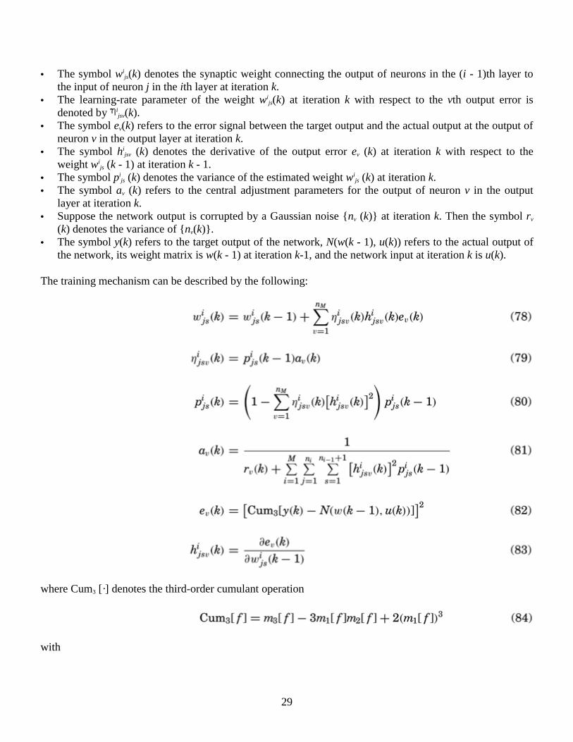
As multilayer feedforward neural networks have become generally recognized as a suitable architecture for representing unknown nonlinearities in dynamic systems, numerous algorithms for training the networks on the basis of observable input-output information have been developed by many researchers. In this article, a training algorithm for neural networks called the cumulant-based weight-decoupled extended Kalman filter (CWDEKF) is described (25). Third-order cumulants are employed to define output errors for the network training. By this means, Gaussian disturbances or non-Gaussian noises with symmetric probability density function among the output signals can be rejected in the cumulant domain. Thus we can obtain clean neural network output information for nonlinear mapping implementation. The weight-decoupled extended Kalman filter training algorithm is applied because it provides faster convergence (learning rate) then other training algorithms. This feature is very important for neural-network-based analysis of nonlinear dynamic systems.
To ease the mathematical burden, we first present a summary of the notation used in the network learning algorithm.
Notation
• The index i refers to different layers in the network, where 1 i M, and M is the total number of layers (including the hidden and output layers) in the network.
• The index j refers to different neurons in the ith layer, where 1 j ni, and ni is the neuron number of the ith layer.
• The index s refers to different neurons in the (i - 1)th layer, where 1 s ni-1 + 1. • The index v refers to different neurons in the output layer, where 1 v nM. • The iteration index k refers to the kth training pattern (example) presented to the network.
29
• The symbol wijs(k) denotes the synaptic weight connecting the output of neurons in the (i - 1)th layer to
the input of neuron j in the ith layer at iteration k. • The learning-rate parameter of the weight wi
js(k) at iteration k with respect to the vth output error is denoted by i
jsv(k). • The symbol ev(k) refers to the error signal between the target output and the actual output at the output of
neuron v in the output layer at iteration k. • The symbol hi
jsv (k) denotes the derivative of the output error ev (k) at iteration k with respect to the weight wi
js (k - 1) at iteration k - 1. • The symbol pi
js (k) denotes the variance of the estimated weight wijs (k) at iteration k.
• The symbol av (k) refers to the central adjustment parameters for the output of neuron v in the output layer at iteration k.
• Suppose the network output is corrupted by a Gaussian noise {nv (k)} at iteration k. Then the symbol rv (k) denotes the variance of {nv(k)}.
• The symbol y(k) refers to the target output of the network, N(w(k - 1), u(k)) refers to the actual output of the network, its weight matrix is w(k - 1) at iteration k-1, and the network input at iteration k is u(k).
The training mechanism can be described by the following:
where Cum3 [·] denotes the third-order cumulant operation
with
30
where pp is the sample number.
A number of network initialization procedures have been developed for general feedforward networks (26, 27). These algorithms are based on linear-algebraic methods to determine the optimal initial weights. With the optimal initial weights, the initial network error is much smaller, thus speeding up the overall training procedure (26, 27). In this article, a conventional randomized-weight initialization procedure is presented:
1.Weights are initialized as random numbers with normal distribution, typically in the range of ±0.1. 2.We initialize the matrices Pi (k):{pi
js (k)} and R(k):{rv (k)} as Pi (0) = 100.0I and R(0) = I, where I refers to the unit matrix.
Thereafter, the CWDEKF algorithm can be applied to train the neural network on which the nonlinear representation is based.
A recurrent neural network differs from a multilayer feedforward neural network in that it has at least one feedback loop, which represents the dynamical characteristics of the network. For example, a recurrent network may consist of a single layer of neurons with each neuron feeding its output signals back to the inputs of all the other neurons. In this structure, there are no self-feedback loops in the network. Self-feedback refers to a situation where the output of a neuron is fed back to its own input. The feedback connections originate from the hidden neurons as well as the output neurons. The presence of feedback loops has a profound influence on the learning capability of the network and on its dynamical performance. Moreover, the feedback loops involve the use of special branches composed of unit-delay elements, which result in nonlinear dynamical behavior by virtue of the nonlinear nature of the neurons. Nonlinear dynamics plays a key role in the storage function of a recurrent network.
The Hopfield network is a typical recurrent network that is well known for its capability of storing information in a dynamically stable configuration. It was Hopfield's paper (28) in 1982, elaborating the remarkable physical capacity for storing information in a dynamically stable network, that sparked off the research on neural networks on the eighties. One of the most fascinating findings of his paper is the realization of the associative memory properties. This has now become immensely useful for pattern recognition.
Physically, the Hopfield network operates in an unsupervised fashion. Thus, it may be used as a content-addressable memory or as a computer for solving optimization problems of a combinatorial kind. The classical traveling-salesman problem is a typical example. Koch applied Hopfield networks to the problem of vision. There has been other work on depth computation and on reconstructing and smoothing images.

31
In tackling a combinatorial optimization problem we are facing a discrete system that has an extremely large but finite number of possible solutions. The task is to find one of the optimal solutions through minimizing a cost function, which provides a measure of system performance. The Hopfield network requires time to converge to an equilibrium condition. The time required depends on the problem size and the possible stability problem. Hence it is never used online unless special-purpose hardware is available for its implementation.
The operational procedure for the Hopfield network may be summarized as follows:
1.Storage (Learning). Let 1, 2, , p denote a known set of N-dimensional memories. Construct the network by using the outer-product rule to compute the synaptic weights of the network as
where wji is the synaptic weight from neuron i to neuron j. The elements of the vector equal ±1. Once they are determined, the synaptic weights are kept fixed.
2.Initialization. Let X denote an unknown N-dimensional input vector presented to the network. Thealgorithm is initialized by setting
where sj (0) is the state of neuron j at time n = 0, and xj is the jth element of the vector X. 3.Iteration until Convergence. Update the elements of the state vector sj (n) asynchronously (i.e., randomly
and one at a time) according to the rule
Repeat until the state vector s remains unchanged. 4.Outputting. Let sf denote the fixed point (stable state) computed at the end of step 3. The resulting output
vector y of the network is
It is clear that a neural network is a massively parallel-distributed network that has a natural capacity for storing experimental knowledge and making it available for use.
The primary characteristics of knowledge representation are twofold: (1) what information is actually made explicit, and (2) how the information is physically encoded. In real-world applications of intelligent machines, neural networks represent a special and versatile class of modeling techniques that are

32
significantly different from conventional mathematical models. Neural networks also offer a convenient and reliable approach for the modeling of highly nonlinear multiinput multioutput systems.
[EEEE Home] [A to Z] [Subjects] [Search]
Copyright ©1999-2000 by John Wiley & Sons, Inc. All rights reserved.

33
MODEL-FREE REPRESENTATION
The traditional qualitative modeling techniques discussed above focus on means for abstracting the value spaces of variables that are used to represent system input-output relationships as well as system states and for simplifying the constraints that hold among the values of those variables. It is obvious that no general nonlinear representations exist for modeling an arbitrary nonlinear system. The approximation accuracy of a nonlinear model depends on what physical system is modeled and what type of model is used. In some cases, where all possible nonlinear models are found to be unsuitable, model-free representations for nonlinear systems will be a better alternative. Rather than a model-based methodology, a flexible model-free technique based on signal processing provides a set of enhanced, sensitive, and definitive characterizations of nonlinear systems. Higher-order statistics have been found to be useful in such analyses (29).
Given an arbitrary real, stationary random signal {y(t)} at the discrete times t = 0, ±1, ±2, , its second-order moment (SOM) My
2 (m) and third-order moment (TOM) My3 (m, n) provide a measure of how the
sequence is correlated with itself at different time points:
where m is the time lag; m, n = 0, ±1, ±2, ; and E[·] denotes statistical expectation. Third-Order Cumulant in Time Domain
For the random signal {y(t)}, its third-order cumulant (TOC) Cy3 (m, n) is given by
Note that the SOM My2 (m) in Eq. (90) is a symmetric function about m = 0, that is, My
2 (-m) = My2 (m).
Hence, My2(m) is a zero-phase function, which means that all phase information about y(t) is lost in My
2(m). With regard to the TOC Cy
3 (m, n), important symmetry conditions follow from the properties of SOM and TOM and Eq. (92):
Thus Cy3 (m, n) is a phase-bearing function, and knowing the TOC in any of the six sectors delimited by Eq.
(93) would enable us to find it everywhere.
34
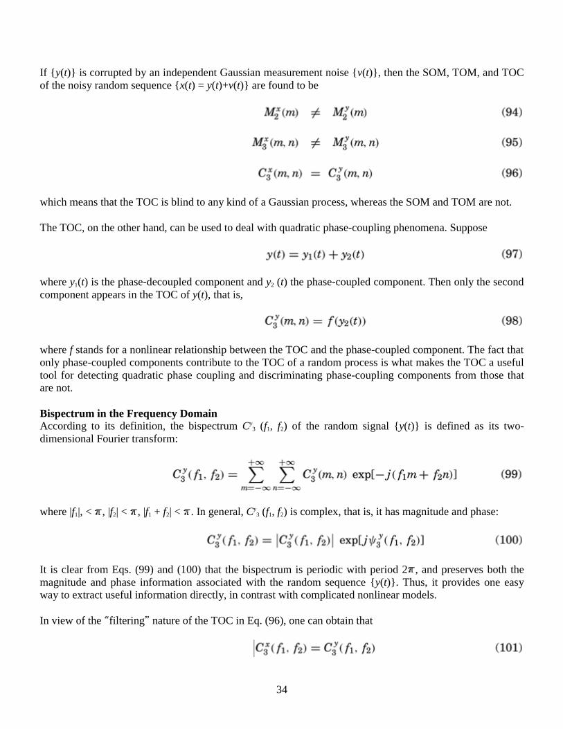
If {y(t)} is corrupted by an independent Gaussian measurement noise {v(t)}, then the SOM, TOM, and TOC of the noisy random sequence {x(t) = y(t)+v(t)} are found to be
which means that the TOC is blind to any kind of a Gaussian process, whereas the SOM and TOM are not.
The TOC, on the other hand, can be used to deal with quadratic phase-coupling phenomena. Suppose
where y1(t) is the phase-decoupled component and y2 (t) the phase-coupled component. Then only the second component appears in the TOC of y(t), that is,
where f stands for a nonlinear relationship between the TOC and the phase-coupled component. The fact that only phase-coupled components contribute to the TOC of a random process is what makes the TOC a useful tool for detecting quadratic phase coupling and discriminating phase-coupling components from those that are not. Bispectrum in the Frequency Domain According to its definition, the bispectrum Cy
3 (f1, f2) of the random signal {y(t)} is defined as its two-dimensional Fourier transform:
where |f1|, < , |f2| < , |f1 + f2| < . In general, Cy3 (f1, f2) is complex, that is, it has magnitude and phase:
It is clear from Eqs. (99) and (100) that the bispectrum is periodic with period 2 , and preserves both the magnitude and phase information associated with the random sequence {y(t)}. Thus, it provides one easy way to extract useful information directly, in contrast with complicated nonlinear models.
In view of the filtering nature of the TOC in Eq. (96), one can obtain that
35
Bearing Eq. (98) in mind, the bispectrum of y(t) can be easily obtained as
where g stands for a nonlinear relationship between the bispectrum and the phase-coupled component. The above discussion has shown that the TOC and bispectrum statistical measures provide an enhanced system characterization capability over conventional second-order measures. As a result, model-free TOC- and bispectrum-based analysis techniques are particularly suitable for extracting internal chararacteristics of a nonlinear system.
[EEEE Home] [A to Z] [Subjects] [Search]
Copyright ©1999-2000 by John Wiley & Sons, Inc. All rights reserved.

36
FEATURES OF NONLINEAR REPRESENTATIONS
Identifiability Identifiability is a concept that is central in system identification problems. Loosely speaking, the problem is whether the system modeling procedure will yield a unique value of the parameter and whether the resulting model is faithful to the true system. The issue involves whether the measured data set is informative enough to distinguish between different models as well as properties of the model structure itself: If the data are informative enough to distinguish between unequal models, then the question is whether different values of parameters can give equal models. Depending on the availability of system information, the corresponding models can be distinguished as: (1) gray-box models, whose structures are known on physical grounds but that have certain of parameters to be estimated from observed data; and (2) black-box models, whose structures as well as parameters are totally unavailable. In the following, we define different kinds of identifiability corresponding to different models.
Definition 1 A gray-box model (y(t), u(t), ), where the observed input-output pair {y(t), u(t)} is given, is internally identifiable at parameter vector * if (y(t), u(t), ) = (y(t), u(t), *), , leads to = *, where comprises the true parameters of the model, and * their estimates. A gray-box model (y(t), u(t), ) is globally internally identifiable if it is internally identifiable at almost all * . Moreover, the gray model
(y(t), u(t), ) is blindly internally identifiable if its input u(t) is unknown.
Definition 2 A black-box model (y(t), u(t)), where the observed input-output pair {y(t), u(t)} is given, is externally identifiable if there exists a determined model structure and parameters such that (y(t), u(t)) = (y(t), u(t), ), . A black-box model (y(t), u(t)) is globally externally identifiable if it is externally identifiable at almost all u u, y y.
A nonlinear differential algebraic representation (7) and a state-space representation (46) are globally internally identifiable if and only if one can obtain differential equations in the form
where i=1, 2, , , n, by differentiating, adding, scaling and multiplying the equations (7) and (46). Then the identification algorithm gives the parameter estimate (30)
As a special case of Eq. (46), a bilinear model (49) is internally identifiable if the above condition (103) is satisfied.

37
For the Volterra representation, it should be pointed out, there is no general identifiability principle. However, if we consider the finite-support Volterra model (34) excited by a zero-mean Gaussian signal, then the model is globally internally identifiable if and only if the power spectral process of the input signal is nonzero at at least t distinct frequencies (31). Moreover, if we consider the finite-support second-order Volterra model (37) excited by an unknown arbitrary zero-mean independent and identically distributed (i.i.d.) random signal, then the model is of blind internal identifiability if and only if the following equation has a unique solution (25):
and
where
and

38

39
where Cy3(m,n) is the TOC of the output signal y(t) defined in Eq. (92), and iuγ , i=2, 3, 4, 6, is the ith-order
autocorrelation of the input u(t). Clearly, one must estimate the (q + 1)2 TOCs Cy3(m,n) for 0 m,n q, and
then invert the equations to solve for the unknown quantities (i,j). This inversion involves solving (q + 1)2 simultaneous cubic equations with (q + 1)2 unknowns. The parameter-coupled terms in Eq. (105) are of high complexity, and conventional model-based estimation theories cannot directly applied. However, the following theorem provides a possible way to estimate the model parameters based on neural networks: Let (m,n) M p and Hij H q, where Hij =[h(0,0) h(0,1) h(0,q) h(q,0) h(q,1) h(q,q)] be open. Let g be continuous on M × H. Consider the equation (105).
Theorem 3 Let DHijg( ij, ) be nonsingular for ij, H and M. Given the class of neural networks, N, that map p × q to q, there exist 1, 2 > 0 and a neural network NN N such that, given > 0,
where = {(Cy3(m,n), (m,n)) : |Cy
3(m,n) - g( ij, )|< 1,|(m,n) - | < 2}. As far as the identifiability of NARMA models is concerned, Eqs. (103) and (104) are also suitable, because a NARMA model is a special type of nonlinear differential algebraic representation and can be characterized by a state-space representation. On the other hand, relying on the approximation capabilities of multilayer neural networks, the functions in Eq. (65) can be approximated by a neural network with appropriate input and output dimensions. This can be stated as the following theorem (32).
Theorem 4 For generic , the input-output behavior of the NARMA model (65) is externally identifiable with arbitrary precision by a multilayer feedforward neural-network-based input-output model of the form
where NN(·) is a multilayer feedforward neural network with 2l inputs and one output characterizing the monitored nonlinear system. Here l is the order of the model.
An important problem faced herein is the choice of the most suitable network topology to perform the identification and modeling of unknown nonlinear dynamic systems efficiently. It mainly lies in the choice of the optimal number of neurons for each of the networks employed, which plays a crucial role in network performance. Considering the external identifiability of fuzzy-logic models, the following theorem shows that the fuzzy-logic models with fuzzifier and defuzzifier are capable of uniformly approximating any nonlinear function over U to any degree of accuracy if U is compact (33).
Theorem 5 For any given real continuous function g on a compact set U n and arbitrary > 0, there exists a fuzzy-logic model f such that

40
This theorem provides a justification for applying the fuzzy-logic representations to almost any nonlinear modeling problem. It also provides an explanation for the practical success of the fuzzy logic models in engineering applications.
Some nonlinear systems are very difficult, if not impossible, to describe with analytical equations. Hence, there is a great need to develop a robust and less model-dependent methodology for the representation of a complex nonlinear dynamic system. To avoid the difficulties of the classical nonlinear-system modeling approach, neural-network-based modeling methods for nonlinear systems have been proposed recently. The main motivation is that any nonlinear relationship can be approximated by a neural network given suitable weighting factors and architecture. Another important property of such networks is their self-learning ability: a neural network can extract the system features from previous training data through learning, whilst requiring little or no a priori knowledge about the system. This provides great flexibility for modeling general nonlinear physical systems and guarantees robust external identifiability of neural-network-based system representations. A multilayer network trained with the CWDEKF algorithm may be viewed as a practical vehicle for performing general nonlinear input-output mapping, due to the following universal approximation theorem (24, 34).
Theorem 6 Let (·) be a nonconstant, bounded, and monotone-increasing continuous function. Let Ip denote the p-dimensional unit hypercube [0,1]p. The space of continuous functions on Ip is denoted by C(Ip). Then, given any function f C(Ip) and > 0, there exist an integer M and sets of real constants j, i, and wij, where i=1, 2,
, M and j=1, 2, , p, such that we may define
as an approximate realization of the function f(·); that is, |F(x1, x2, , xp) - f(x1, x2, , xp)| < for all (x1, x2, , xp) Ip.
This theorem is directly applicable to multilayer networks. We first note that the logistic function used as the nonlinearity in a neuron node for the construction of a multilayer network is indeed a nonconstant, bounded, and monotone-increasing function. It therefore satisfies the conditions imposed on the function (·). Next, we note that the above equation represents the output of a multilayer network described as follows: (1) the network has p point nodes and a single hidden layer consisting of M neurons; the inputs are denoted by (x1, x2, , xp); (2) hidden neuron i has synaptic weights (wi1, Wi2, , wip) and threshold i; and (3) the network output is a linear combination of the outputs of the hidden neurons, with ( 1, 2, M) as coefficients.
The universal approximation theorem 6 is an existence theorem in the sense that it provides the mathematical justification for the approximation of an arbitrary continuous function as opposed to exact representation.
Controllability Controllability is one of the most important properties of systems modeled by state-space representations. A state-space model in Eq. (46) is said to be controllable if an available input u(t) is sufficient to bring the

41
model from any initial state x(0) to any desired final state x(t). The importance of controllability in the formulation of the control problems for linear systems is evident. A linear time-invariant system (t) = Ax(t) + Bu(t) is completely controllable if and only if the matrix E = [B AB An-1 B] has rank n, where x(t) n, u(t) m.
In spite of many attempts to characterize controllability for nonlinear systems, similar generic results to those available for linear systems do not exist for nonlinear systems. Hence, the choice of controller models for nonlinear systems is a formidable problem, and successful control has to depend on several strong assumptions regarding the input-output behavior of the systems. For example, we consider the specified (affine) nonlinear model of the form
where x(t) = [x1,x2, , xn]T is the local coordinate on a smooth n-dimensional manifold M, the control u(t) is a scalar piecewise smooth function, and f(x, t), g(x, t) are the local coordinate representations of smooth vector fields globally defined on M. The model (110) is locally controllable at an equilibrium point xe of f(·) if [B, AB, , An-1 B] has full rank, where B = g(xe) and A = f(xe)/ x (36).
On the other hand, the variable structure of bilinear systems allows them to be more controllable than linear systems, just as it frequently provides for a more accurate model. Let us consider the bilinear system given by Eq. (49). It is assumed that the class of admissible inputs u(t) is the class of all piecewise continuous vector time functions with [0, ) and range U, where U is a compact connected set containing the origin in
m. The reachable zone from an initial state x0, R(x0) n, is the set of all states to which the system can be transferred in finite time, starting at x0. Similarly, the incident zone to a terminal state xf, I(xf) n, is the set of all initial states from which xf is reachable in finite time.
For each fixed x U, the bilinear system is a constant-parameter linear system with system matrix F + m
i=1Niui. The term mi=1Niui in the system matrix permits manipulation of the eigenvalues of the fixed-control
system. With an appropriate controller it is often possible to shift these eigenvalues from the left half of the complex plane to the right half. The controllability analysis presented here can be summarized by the following sufficient conditions (5):
Theorem 7 The bilinear system (49) is completely controllable if: (1) there exist input values u+ and u- such that the real parts of the eigenvalues of the system matrix are positive and negative, respectively, and such that equilibrium states xe(u+) and xe(u-) are contained in a connected component of the equilibrium set, and (2) for each x in the equilibrium set with an equilibrium input ue(x) U such that f(x, ue(x)) = 0, there exists a v Rm such that g lies in no invariant subspace of dimensional at most n - 1 of the matrix E, where

42
As one might expect, the conditions given by the above theorem are not as simple as the popular conditions for complete controllability of linear systems. For phase-variable systems, x1 = x, x2 = , , xn = x(n-1), condition (2) is always satisfied if G is a nonzero matrix. Condition (2) is satisfied if all the eigenvalues of the system matrix F + m
i=1Niui can be shifted across the imaginary axis of the complex plane without passing through zero, as u ranges continuously over a subset of U.
Observability A nonlinear state-space model is said to be observable if, given any two states x1, x2, there exists an input sequence of finite length, ul = [u(0), u(1), , u(l)]T, such that yl(x1, ul) yl(x2, ul), where yl is the output sequence. The ability to effectively estimate the state of a model or to identify it based on input-output observations is determined by the observability properties of the model.
Observability has been extensively studied in the context of linear systems and is now part of the standard control literature. An nth-order single-input and single-output time-invariant linear system is described by the set of equations
where x(t) n, u(t) , y(t) , A is an n × n matrix, and B, C are n-dimensional vectors. A basic result in linear control theory states that the above system will be observable if and only if the n × n matrix M = [C CA CAn-1]T is of rank n. M is called the observability matrix. If the system (112) is observable and [CB CAB CAd-2 B]T = 0, but CAd-1B 0, then we have y(t + d) = CAd x(t) + CAd-1Bu(t). This implies that the input at any instant t can affect the output only d instants later, where d denotes the delay in the propagation of the signals through the system and is called the relative degree of the system.
Observability of a linear system is a system-theoretic property and remains unchanged even when inputs are present, provided they are known. For an observable linear system of order n, any input sequence of length n will distinguish any state from any other state. If two states are not distinguishable by this randomly chosen input, they cannot be distinguished by any other input sequence. In that case, the input-output behavior of the system can be realized by an observable system of lower dimension, where each state in the new system represents an equivalence class that corresponds to a set of states that could not be distinguished in the old one.
Whereas a single definition is found to be adequate for linear time-invariant systems, the concept of observability is considerably more involved for nonlinear systems. A desirable situation would be if any input sequence of length l sufficed to determine the state uniquely, for some integer l. This form of observability will be referred to as strong observability. It readily follows that any observable linear system is strongly observable with l = n, n being the order of the system. A less restrictive form of observability is the notion of generic observability. A system of the form (46) is said to be generically observable if there exists an integer l such that almost any input sequence of length greater or equal to l will uniquely determine the state.
Now let us look at the observability of nonlinear systems using Eq. (46). This problem arises when the laws governing the system are known but the states of the system are not accessible or only partly accessible. By

43
definition, complete knowledge of the states will enable accurate prediction of the system's behavior. Thus the observation problem in this case actually reduces to the estimation of the state based on input and output observations over a time interval [t0, t0 + l], or in other words establishing an observer. Sufficient conditions for strong local observability of a system (46) around the origin can be derived from the observability properties of its linearization at the origin:
where A = fx|0,0, B = fu|0,0, C = gx|0 are the system's Jacobian matrices. This is summarized by the following theorem (33). Theorem 8 Let be nonlinear system (45), and l its linearization around the equilibrium as given in Eq. (113). If l is observable, then is locally strongly observable.
A bilinear model (49) or (50) is called observable if there are no indistinguishable states in the model. Theorem 9 gives a necessary and sufficient condition for observability of bilinear models (8).
Theorem 9 The bilinear model described in Eq. (49) or (50) is observable if and only if rank Qn = n, where Qn = [q1, q2,
, qn]T, q1 = C, qi = [qi-1F qi-1Ni]T, i = 2, 3, , n.
[EEEE Home] [A to Z] [Subjects] [Search]
Copyright ©1999-2000 by John Wiley & Sons, Inc. All rights reserved.
44
EXAMPLE
This example shows how a neural network together with a nonlinear model approach is used for short-term electric load forecasting (35). This neural-network model utilizes the full dynamic range of the neural network and is a nonlinear model for nonstationary time series. The model is used to provide hourly load forecasts one day ahead. Off-line simulation has been done on the Hong Kong Island electric load profile provided by the Statistics and Planning Division of Hong Kong Electric Company Limited.
The electric load forecast models can be summarized in the following two equations: for a static model (feedforward neural network),
and for a dynamical model (recurrent neural network),
where xt is the load consumption, t+l is the weather forecast, wt is the weather information, and et is a noise residual at time t. The nonlinear function h is nonlinearly approximated by ANN. From the above models, the load forecast t+l is estimated mainly from the currently available load profile.
In general, a linear time series {xt} can be written in the form of an ARMA model as
where B is the backward shift operator, and the autoregressive operator (B) of order p is given by
The moving-average operator (B) of order q is defined by
where the white noise et with finite variance 2 is zero-mean, i.i.d., and independent of past xt. Equation (114) can be rewritten in the form

45
If the roots of the equation
lie outside the unit circle, the time series {xt} is stationary; otherwise {xt} is nonstationary. For linear nonstationary time series {xt}, the ARMA model for stationary time series can still be used, but the above ARMA model (115) has to be reformulated as
or
where dxt = (1 - Bd)xt = xt - xt-d and i = i + i+d. The model (116) is the so-called ARIMA model. A natural generalization of the linear ARIMA model to the nonlinear case would be the nonlinear autoregressive integrated moving average (NARIMA) model, which is given by
or
where h is an unknown smooth function and, as in Eq. (114), it is assumed that the white noise et with variance 2 is zero-mean, i.i.d, and independent of past xt. The minimum-mean-squared-error optimal predictor of xt given xt-1, , xt-r is the conditional expectation
This predictor has mean squared error 2. In this work, a nonlinear autoregressive integrated (NARI) model, the special case of the NARIMA, is considered and is defined by
or
46
We focus on a multilayer feedforward neural network (FNN) and how it may be used to forecast the hourly load consumption of the coming day. In many time-series predictions, the time-series model is based on nonlinear autoregressive (NAR) models of the form
The neural STLF model can be considered as a modified NAR model given by
and the unknown smooth function h is nonlinearly approximated by a FNN. Hence, the neural optimal predictor is given by
where 0 l 24 and the function is a smooth bounded monotonic function, tanh(0.5x). The vector wt of m components contains the available weather information at time t. The parameters W0
ij, W0ik, and W1
i are the neural-network weights.
To obtain an accurate load forecast, we should identify the most appropriate model in accordance with the nature of load consumption. In this example, the modified NARI model in Eq. (118b) is proposed for STLF. Several important weather factors are also included, because weather variation is one of the crucial disturbances to electric load demand. Consequently, the modified NARI model for STLF is given by
and the neural optimal predictor is then formulated by
where 0 l 24. The weather information vector wt contains four components, namely, temperature, relative humidity, level of rainfall, and level of sunshine.
The architecture of our proposed neural network model is illustrated in Fig. 9(b). The structure of the modified NAR model for STLF is depicted in Fig. 9(a). This type of NARI neural-network model is called a weather compensation neural network because the weather-dependent component will be only determined from the weather information and load consumption of the previous day.

47
The characteristics of electric load consumption gradually change because of many uncontrollable factors. Our weather compensation neural network (NARI model), without keeping track of the change of load characteristic, will degrade in forecasting performance over the years. An adaptive tracking scheme is therefore proposed so that the weather compensation neural network will be retrained every day. This scheme can efficiently update the neural network to adapt to the changing conditions of the environment. Different sizes of window of the trained set have been studied. The size of the window determines the memory of past knowledge. Too small a window may produce catastrophic loss of information that severely degrades the forecasting performance and robustness. Three different sizes - 10 days, 20 days, and 136 days - are examined. Updating is omitted when the standard deviation of the forecast error is less than 990 MW. The results are depicted in Fig. 10, and they show that the neural network provides the most robust forecasting when the window size of 136 days is used. Figure 11 displays a comparison of the actual load and the load forecast for seven consecutive working days using our proposed NARI neural network and adaptive tracking scheme. Figures 12 and 13 display a comparison of the actual load and the load forecast for the worst cases using the NAR and the NARI neural network, respectively.
[EEEE Home] [A to Z] [Subjects] [Search]
Copyright ©1999-2000 by John Wiley & Sons, Inc. All rights reserved.

48
CONCLUDING REMARKS
Nonlinear system representations are classified by a simple dichotomy: a system is represented either linearly or nonlinearly. The number and variety of nonlinear representations is almost limitless, and one does not find the complete and elegant theory that exists for linear representations. It would be expecting too much if one hoped to find a universal analytical technique applicable to any nonlinear system representation with an arbitrary input signal.
In this article, we have discussed several nonlinear representations and their important features such as identifiability, controllability, and observability. These representations are widely used in signal processing, circuit systems, control systems, and communication systems. A comparison of these representations is given in Table 1. It can be seen that, with different types of input signal, different nonlinear representations should be selected. When internal identifiability is important, Volterra, state-space, and bilinear representations are the better choices, due to the linear parameter relationship of the Volterra system and the compact description of the state-space and bilinear systems. For external identifiability, fuzzy logic and neural-network-based representations often appear to be useful for characterizing nonlinear systems in a black-box approach.
On the other hand, a state-space representation can be used to guarantee high controllability and observability, since the corresponding theories in the linear domain can be extended to the nonlinear world. For system inversion, no one representation is the best, due to the complexity of the problem; but suboptimal alternatives may be obtained with Volterra, state-space, or bilinear representations.
[EEEE Home] [A to Z] [Subjects] [Search]
Copyright ©1999-2000 by John Wiley & Sons, Inc. All rights reserved.

49
ACKNOWLEDGMENT
The authors would like to thank the Hong Kong Electric Company Limited for providing the electric load data and weather information for this part of work.
[EEEE Home] [A to Z] [Subjects] [Search]
Copyright ©1999-2000 by John Wiley & Sons, Inc. All rights reserved.

50
FIGURES AND TABLE

51

52
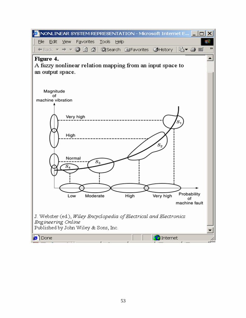
53

54

55
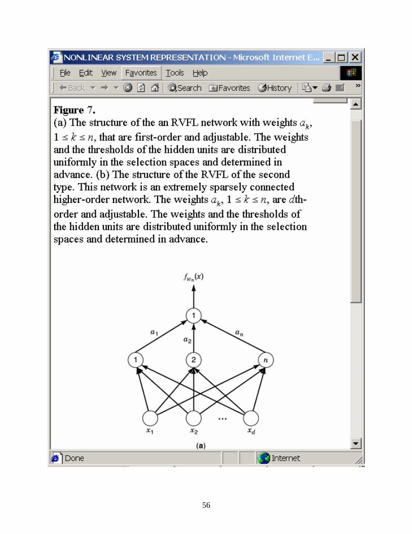
56

57

58

59

60

61
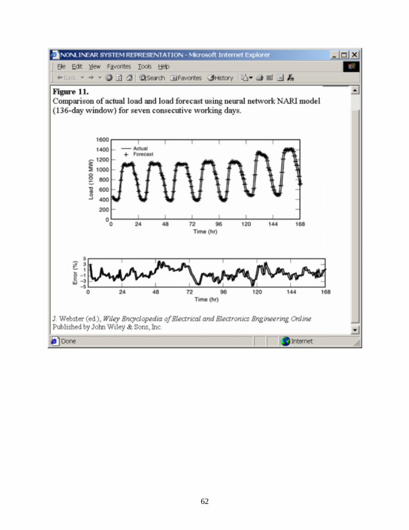
62

63
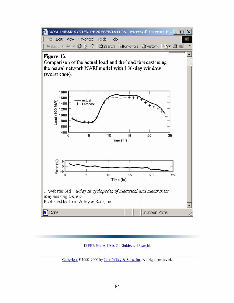
64
[EEEE Home] [A to Z] [Subjects] [Search]
Copyright ©1999-2000 by John Wiley & Sons, Inc. All rights reserved.

65
Table 1. Comparison of Different Nonlinear Representations
Representation Input Signals Identifiability Controllability Observability Differential algebraic
Deterministic √ х х
Volterra Random √ х х State-space Deterministic
or random √ √ √
Bilinear Deterministic or random
√ √ √
NARMA Random √ х х Fuzzy logic Deterministic √ х х
Neural network Deterministic or random
√ х х
J. Webster (ed.), Wiley Encyclopedia of electrical and Electronics Engineering Online Published by John Wiley & Sons, Inc.
[EEEE Home] [A to Z] [Subjects] [Search]
Copyright ©1999-2000 by John Wiley & Sons, Inc. All rights reserved.