nonlinear relationships - university of notre damerwilliam/stats2/l61.pdf · and the relationship...

Nonlinear Relationships

Nonlinear relationships Richard Williams, University of Notre Dame, https://www3.nd.edu/~rwilliam/

Last revised February 20, 2015

Sources: Berry & Feldman’s Multiple Regression in Practice 1985; Pindyck and Rubinfeld’s Econometric Models and Economic Forecasts 1991 edition; McClendon’s Multiple Regression and Causal Analysis, 1994; SPSS’s Curvefit documentation. Also see Hamilton’s Statistics with Stata, Updated for Version 9, for more on how Stata can handle nonlinear relationships.

Linearity versus additivity. Remember again that the general linear model is

Y X X X X E Y Xj j j k kj j i ij ji

k

j j= + + + + + = + + = +=∑α β β β ε α β ε ε1 1 2 2

1

... ( | )

The assumptions of linearity and additivity are both implicit in this specification.

• Additivity = assumption that for each IV X, the amount of change in E(Y) associated with a unit increase in X (holding all other variables constant) is the same regardless of the values of the other IVs in the model. That is, the effect of X1 does not depend on X2; increasing X1 from 10 to 11 will have the same effect regardless of whether X2 = 0 or X2 = 1.

• With non-additivity, the effect of X on Y depends on the value of a third variable, e.g. gender. As we’ve just discussed, we use models with multiplicative interaction effects when relationships are non-additive.

• Linearity = assumption that for each IV, the amount of change in the mean value of Y associated with a unit increase in the IV, holding all other variables constant, is the same regardless of the level of X, e.g. increasing X from 10 to 11 will produce the same amount of increase in E(Y) as increasing X from 20 to 21. Put another way, the effect of a 1 unit increase in X does not depend on the value of X.

• With nonlinearity, the effect of X on Y depends on the value of X; in effect, X somehow interacts with itself. This is sometimes refered to as a self interaction. The interaction may be multiplicative but it can take on other forms as well, e.g. you may need to take logs of variables. Examples:

http://www3.nd.edu/%7Erwilliam/


Dealing with Nonlinearity in variables. We will see that many nonlinear specifications can be converted to linear form by performing transformations on the variables in the model. For example, if Y is related to X by the equation

E Y Xi i( ) = +α β 2

and the relationship between the variables is therefore nonlinear, we can define a new variable Z = X2. The new variable Z is then linearly related to Y, and OLS regression can be used to estimate the coefficients of the model. There are numerous other cases where, given appropriate transformations of the variables, nonlinear relationships can be converted into models for which coefficients can be estimated using OLS. We’ll cover a few of the most important and common ones here, but there are many others.

Detecting nonlinearity and nonadditivity. The key question is whether the slope of the relationship between an IV and a DV can be expected to vary depending on the context.

• The first step in detecting nonlinearity or nonadditivity is theoretical rather than technical. Once the nature of the expected relationship is understood well enough to make a rough graph of it, the technical work should begin. Hence, ask such questions as, can the slope of the relationship between Xi and E(Y) be expected to have the same sign for all values of Xi? Should we expect the magnitude of the slope to increase as Xi increases, or should we expect the magnitude of the slope to decrease as Xi increases?

• Can do scatterplots of the IV against the DV. Sometimes, nonlinearity will be obvious.

• Can often do incremental F tests or Wald tests like we have used in other situations. Stata’s estat ovtest command can also be used in some cases; see below.

Types of nonlinearity

1. Polynomial models. Some variables have a curvilinear relationship with each other. Increases in X initially produce increases in Y, but after a while subsequent increases in X produce declines in Y, e.g.

Y0N0

X1

43210-1-2-3-4

2

0

-2

-4

-6

-8

-10

Observed

Linear

Quadratic

YEXP

X1

43210-1-2-3-4

30

20

10

0

-10

Observed

Linear

Exponential


Polynomial models can estimate such relationships. A polynomial model can be appropriate if it is thought that the slope of the effect of Xi on E(Y) changes sign as Xi increases. For many such models, the relationship between Xi and E(Y) can be accurately reflected with a specification in which Y is viewed as a function of Xi and one or more powers of Xi, as in

Y X X X XMM= + + + + + +α β β β β ε1 1 2 1

23 1

31...

The graph of the relationship between X1 and E(Y) consists of a curve with one or more “bends”, points at which the slope of the curve changes signs. The numbers of bends nearly always equals M - 1. For M = 2, the curve bends (changes sign) when X1 = -b1/2b2. If this value appears within the meaningful range of X, the relationship is nonmonotonic. If this value falls outside the meaningful range of X, the relationship appears monotonic (i.e. Y always decreases or increases as X increases.)

This model is easily estimated — simply compute X2 = X12, X3 = X13, etc., and regress Y on these terms. (In practice, we usually stop at M =2 or M = 3). Or, in Stata 11 or higher, use factor variables, e.g. c.x1#c.x1 (equivalent to X12), c.x1#c.x1#c.x1 (equivalent to X13).

Example: In psychology, the Yerkes-Dodson law predicts that the relationship between physiological arousal and performance will follow an inverted U-shaped function, i.e. higher levels of arousal initially increase performance, but after a certain level of arousal is achieved additional arousal decreases performance.

INTERPRETATION. When M = 2, the b1 coefficient indicates the overall linear trend (positive or negative) in the relationship between X and Y across the observed data. The b2 coefficient indicates the direction of curvature. If the relationship is concave upward, b2 is positive, if concave downward b2 is negative. For example, a positive coefficient for X and a negative coefficient for X2 cause the curve to rise initially and then fall.

More generally, a polynomial of order k will have a maximum of k-1 bends (k-1 points at which the slope of the curve changes direction); for example, a cubic equation (which includes X, X2, and X3) can have 2 bends. Note that the bends do not necessarily have to occur within the observed values of the Xs.

Y0N0

X1

43210-1-2-3-4

2

0

-2

-4

-6

-8

-10

Observed

Linear

Quadratic


SOME POLYNOMIAL MODELS, WITH QUADRATIC TERMS: [Note: These are often refered to as quadratic models.] b1 positive, b2 positive; Y = 2X + X2

b1 positive, b2 negative; Y = 2X - X2

b1 negative, b2 positive; Y = -2X + X2

b1 negative, b2 negative; Y = -2X - X2

b1 zero, b2 positive; Y = X2

b1 zero, b2 negative; Y = -X2

YPP0

X1

43210-1-2-3-4

20

10

0

-10

Observed

Linear

Quadratic

YPN0

X1

43210-1-2-3-4

10

0

-10

-20

Observed

Linear

Quadratic

YNP0

X1

43210-1-2-3-4

20

10

0

-10

Observed

Linear

Quadratic

YNN0

X1

43210-1-2-3-4

10

0

-10

-20

Observed

Linear

Quadratic

Y0P0

X1

43210-1-2-3-4

10

8

6

4

2

0

-2

Observed

Linear

Quadratic

Y0N0

X1

43210-1-2-3-4

2

0

-2

-4

-6

-8

-10

Observed

Linear

Quadratic


SOME POLYNOMIAL MODELS, WITH CUBIC TERMS: [NOTE: These are often referred to as cubic models.] b1 positive, b2 positive, b3 negative; Y = 2X + X2 - X3

b1 negative, b2 positive, b3 positive; Y = -2X + X2 + X3

b1 zero, b2 zero, b3 positive; Y = X3

b1 zero, b2 zero, b3 negative; Y = - X3

Testing whether polynomial terms are needed. As usual, you can use incremental F tests or Wald tests to test whether polynomial terms belong in a model. In the following example, x2 is x^2, x3 is x^3, and x4 is x^4. . use https://www3.nd.edu/~rwilliam/statafiles/nonlin1.dta, clear . nestreg, quietly: reg y x1 (x2 x3 x4)

YPPN

X1

43210-1-2-3-4

40

30

20

10

0

-10

-20

Observed

Linear

Quadratic

Cubic

YNPP

X1

43210-1-2-3-4

40

30

20

10

0

-10

-20

Observed

Linear

Quadratic

Cubic

Y00P

X1

43210-1-2-3-4

30

20

10

0

-10

-20

-30

Observed

Linear

Quadratic

Cubic

Y00N

X1

43210-1-2-3-4

30

20

10

0

-10

-20

-30

Observed

Linear

Quadratic

Cubic


Block 1: x1 Block 2: x2 x3 x4 +-------------------------------------------------------------+ | | Block Residual Change | | Block | F df df Pr > F R2 in R2 | |-------+-----------------------------------------------------| | 1 | 3.21 1 59 0.0782 0.0516 | | 2 | 34.10 3 56 0.0000 0.6645 0.6129 | +-------------------------------------------------------------+

This shows us that at least one polynomial term should be in the model. Or, using a Wald test,

. quietly reg y x1 x2 x3 x4

. test x2 x3 x4 ( 1) x2 = 0 ( 2) x3 = 0 ( 3) x4 = 0 F( 3, 56) = 34.10 Prob > F = 0.0000

Using factor variable notation, . reg y x1 c.x1#c.x1 c.x1#c.x1#c.x1 c.x1#c.x1#c.x1#c.x1 Source | SS df MS Number of obs = 61 -------------+------------------------------ F( 4, 56) = 27.73 Model | 44318.4937 4 11079.6234 Prob > F = 0.0000 Residual | 22372.3755 56 399.506705 R-squared = 0.6645 -------------+------------------------------ Adj R-squared = 0.6406 Total | 66690.8692 60 1111.51449 Root MSE = 19.988 ------------------------------------------------------------------------------------- y | Coef. Std. Err. t P>|t| [95% Conf. Interval] --------------------+---------------------------------------------------------------- x1 | -5.295304 3.637185 -1.46 0.151 -12.58146 1.990853 | c.x1#c.x1 | .8421613 3.238257 0.26 0.796 -5.644847 7.32917 | c.x1#c.x1#c.x1 | 1.714328 .5977291 2.87 0.006 .5169324 2.911723 | c.x1#c.x1#c.x1#c.x1 | .9803527 .3897181 2.52 0.015 .1996535 1.761052 | _cons | .8290378 4.801439 0.17 0.864 -8.789401 10.44748 ------------------------------------------------------------------------------------- . test c.x1#c.x1 c.x1#c.x1#c.x1 c.x1#c.x1#c.x1#c.x1 ( 1) c.x1#c.x1 = 0 ( 2) c.x1#c.x1#c.x1 = 0 ( 3) c.x1#c.x1#c.x1#c.x1 = 0 F( 3, 56) = 34.10 Prob > F = 0.0000

Stata also provides the estat ovtest command (ov = omitted variables; you can just use ovtest for short). In its default form, ovtest regresses y on yhat^2, yhat^3, and yhat^4. A significant test statistic indicates that polynomial terms should be added. In this particular


example, ovtest gives the same results as above, but that wouldn’t necessarily be true in a more complicated model. . quietly reg y x1 . ovtest Ramsey RESET test using powers of the fitted values of y Ho: model has no omitted variables F(3, 56) = 34.10 Prob > F = 0.0000

As Appendix A explains in more detail, there are various ways to plot the relationship between y and x1. Here I will use the user-written routine curvefit, which “produces curve estimation regression statistics and related plots between two variables for 35 different curve estimation regression models.” Look at the help file to get the codes for the functions you want. In this case I am telling curvefit to fit and display a linear model (function 1) and a 4th order polynomial model (function h). . curvefit y x1, f(1 h) Curve Estimation between y and x1 ------------------------------------------ Variable | Linear Polynomial -------------+---------------------------- b0 | _cons | 20.3918 .82903778 | 4.86 0.17 | 0.0000 0.8635 -------------+---------------------------- b1 | _cons | 4.2672153 -5.2953044 | 1.79 -1.46 | 0.0782 0.1510 -------------+---------------------------- b2 | _cons | .8421613 | 0.26 | 0.7958 -------------+---------------------------- b3 | _cons | 1.7143277 | 2.87 | 0.0058 -------------+---------------------------- b4 | _cons | .98035267 | 2.52 | 0.0148 -------------+---------------------------- Statistics | N | 61 61 r2_a | .0355574 .64057445 ------------------------------------------ legend: b/t/p

These are the same coefficient estimates we got before. Here is the graph produced by curvefit:


That is a little bizarre looking (but then again these are fake data!) In the probably more common case where you just had a squared term, it would look something like this (function 1 = linear, function 4 = quadratic) . curvefit y x1, f(1 4) Curve Estimation between y and x1 ------------------------------------------ Variable | Linear Quadratic -------------+---------------------------- b0 | _cons | 20.3918 -6.4231073 | 4.86 -1.52 | 0.0000 0.1348 -------------+---------------------------- b1 | _cons | 4.2672153 4.2672153 | 1.79 2.66 | 0.0782 0.0100 -------------+---------------------------- b2 | _cons | 8.6499701 | 8.49 | 0.0000 -------------+---------------------------- Statistics | N | 61 61 r2_a | .0355574 .56277883 ------------------------------------------ legend: b/t/p

-50

050

100

150

-4 -2 0 2 4x1

ObservedLinear Fit

4 order Polynomial Fit

Curve fit for y


2A. Exponential models – Growth Models. We often think that variables will increase exponentially rather than arithmetically. For example, each year of education may be worth an additional 5% income, rather than, say, $2,000. Hence, for somebody who would otherwise make $20,000 a year, an additional year of education would raise their income $1,000. For those who would otherwise be expected to make $40,000, an additional year could be worth $2,000. Note that the actual dollar amount of the increase is different, but the percentage increase is the same. Such relationships can often be modeled as

Y e X= + +( )α β ε

When β is positive, the curve has positive slope throughout, but the slope gradually increases in magnitude as X increases. When β is negative, the curve has a negative slope throughout and the slope gradually decreases in magnitude as X increases, with the curve approaching the X axis as Y gets infinitely large. (NOTE: This is often called a growth model.)

When β is positive and small in magnitude (around .25 or less) β * 100 is approximately equal to the percentage increase in E(Y) associated with a unit increase in X, e.g. if β = .10, then a 1 unit increase in X will produce about a 10% increase in E(Y).

Here is a graph of such a relationship. The curved line is a plot of X versus Y, where there is an exponential relationship between the two.

-50

050

100

150

-4 -2 0 2 4x1

ObservedLinear Fit

Quadratic Fit

Curve fit for y


Following is an example of an exponential growth model. It shows the problems that occur if you instead use a linear model of constant growth.

YEXP

X1

43210-1-2-3-4

30

20

10

0

-10

Observed

Linear

Exponential


Exponential (growth) model. Income starts at $10,000 and grows 10% a year, compounded annually Year Income Increase in $ Regr Prediction LN(Income) Increase in ln($) Regr Prediction

1 $ 10,000.00 ($12,279.83) 9.2103404 9.21034 2 $ 11,000.00 $ 1,000.00 ($7,651.47) 9.3056506 0.09531 9.30565 3 $ 12,100.00 $ 1,100.00 ($3,023.11) 9.4009607 0.09531 9.40096 4 $ 13,310.00 $ 1,210.00 $1,605.24 9.4962709 0.09531 9.49627 5 $ 14,641.00 $ 1,331.00 $6,233.60 9.5915811 0.09531 9.59158 6 $ 16,105.10 $ 1,464.10 $10,861.96 9.6868913 0.09531 9.68689 7 $ 17,715.61 $ 1,610.51 $15,490.31 9.7822015 0.09531 9.7822 8 $ 19,487.17 $ 1,771.56 $20,118.67 9.8775116 0.09531 9.87751 9 $ 21,435.89 $ 1,948.72 $24,747.02 9.9728218 0.09531 9.97282

10 $ 23,579.48 $ 2,143.59 $29,375.38 10.068132 0.09531 10.06813 11 $ 25,937.42 $ 2,357.95 $34,003.74 10.163442 0.09531 10.16344 12 $ 28,531.17 $ 2,593.74 $38,632.09 10.258752 0.09531 10.25875 13 $ 31,384.28 $ 2,853.12 $43,260.45 10.354063 0.09531 10.35406 14 $ 34,522.71 $ 3,138.43 $47,888.81 10.449373 0.09531 10.44937 15 $ 37,974.98 $ 3,452.27 $52,517.16 10.544683 0.09531 10.54468 16 $ 41,772.48 $ 3,797.50 $57,145.52 10.639993 0.09531 10.63999 17 $ 45,949.73 $ 4,177.25 $61,773.88 10.735303 0.09531 10.7353 18 $ 50,544.70 $ 4,594.97 $66,402.23 10.830613 0.09531 10.83061 19 $ 55,599.17 $ 5,054.47 $71,030.59 10.925924 0.09531 10.92592 20 $ 61,159.09 $ 5,559.92 $75,658.94 11.021234 0.09531 11.02123 21 $ 67,275.00 $ 6,115.91 $80,287.30 11.116544 0.09531 11.11654 22 $ 74,002.50 $ 6,727.50 $84,915.66 11.211854 0.09531 11.21185 23 $ 81,402.75 $ 7,400.25 $89,544.01 11.307164 0.09531 11.30716 24 $ 89,543.02 $ 8,140.27 $94,172.37 11.402475 0.09531 11.40247 25 $ 98,497.33 $ 8,954.30 $98,800.73 11.497785 0.09531 11.49778 26 $108,347.06 $ 9,849.73 $103,429.08 11.593095 0.09531 11.59309 27 $119,181.77 $ 10,834.71 $108,057.44 11.688405 0.09531 11.68841 28 $131,099.94 $ 11,918.18 $112,685.80 11.783715 0.09531 11.78372 29 $144,209.94 $ 13,109.99 $117,314.15 11.879025 0.09531 11.87903 30 $158,630.93 $ 14,420.99 $121,942.51 11.974336 0.09531 11.97434

Average $ 54,831.34 $ 54,831.34

Note that income increases 10% per year. In absolute terms, the growth is small at first ($1,000 a year) and then gets bigger and bigger ($14,420 in year 30). The linear regression model (left-hand side) predicts a constant growth of about $4,628.36 a year. Hence, it overestimates growth in the early years and underestimates it later. OLS works much better with the exponential growth model (right-hand side), where the dependent variable is the log of income. Note that e.09531 = 1.1, which shows that there is 10% annual growth.

Income Regressed on Year

$(40,000.00)

$(20,000.00)

$-

$20,000.00

$40,000.00

$60,000.00

$80,000.00

$100,000.00

$120,000.00

$140,000.00

$160,000.00

$180,000.00

0 5 10 15 20 25 30 35

Year

Inco

me

Actual IncomePredicted Income

Log Income Regressed on year

8

9

10

11

12

13

0 5 10 15 20 25 30 35

Year

Inco

me

Actual & Predicted Income


Estimation. To estimate the exponential model using OLS: The traditional (but often inferior) approach has been to take the log of both sides of the equation, yielding

lnY X= + +α β ε

We therefore merely compute a new variable which equals ln Y and regress the Xs on it. In Stata we could do something like

. use "https://www3.nd.edu/~rwilliam/statafiles/nonlinln.dta", clear

. gen lninc = ln(inc2)

. reg lninc year Source | SS df MS Number of obs = 30 -------------+------------------------------ F( 1, 28) = 140.03 Model | 18.0405098 1 18.0405098 Prob > F = 0.0000 Residual | 3.60730356 28 .12883227 R-squared = 0.8334 -------------+------------------------------ Adj R-squared = 0.8274 Total | 21.6478134 29 .746476324 Root MSE = .35893 ------------------------------------------------------------------------------ lninc | Coef. Std. Err. t P>|t| [95% Conf. Interval] -------------+---------------------------------------------------------------- year | .0895931 .0075712 11.83 0.000 .0740843 .1051019 _cons | 2.393403 .1278533 18.72 0.000 2.131508 2.655299 ------------------------------------------------------------------------------

The potential problem with this approach is that the log of 0 is undefined; ergo, any cases with 0 (or for that matter negative) values will get dropped from the analysis. Further, most of us don’t think in terms of logs of variables; we would rather see how X is related to the unlogged Y. It is therefor often better to estimate this model:

( )( ) XE Y e α β+= When you do this, Y itself can equal 0; all that is required is that its expected value be greater than zero. In Stata, we can estimate this as a generalized linear model with link log. The commands are . glm inc2 year, link(log) Generalized linear models No. of obs = 30 Optimization : ML Residual df = 28 Scale parameter = 490.7657 Deviance = 13741.44059 (1/df) Deviance = 490.7657 Pearson = 13741.44059 (1/df) Pearson = 490.7657 Variance function: V(u) = 1 [Gaussian] Link function : g(u) = ln(u) [Log] AIC = 9.098184 Log likelihood = -134.4727664 BIC = 13646.21 ------------------------------------------------------------------------------ | OIM inc2 | Coef. Std. Err. z P>|z| [95% Conf. Interval] -------------+---------------------------------------------------------------- year | .0845539 .0114012 7.42 0.000 .0622081 .1068998 _cons | 2.531094 .2774882 9.12 0.000 1.987228 3.074961 ------------------------------------------------------------------------------


In this case, it didn’t make a whole lot of difference in the estimates, but it might matter more if there were some 0 values for income. We can also plot the results. The original values of income, rather than the logged values, are used in the graph. As you can see, the distance between each point keeps getting bigger and bigger (i.e. the growth fit curve keeps getting steeper and steeper), which is what you expect with exponential growth. With curvefit we use function 0 (growth model). . curvefit inc2 year, f(1 0) Curve Estimation between inc2 and year ------------------------------------------ Variable | Linear Growth -------------+---------------------------- b0 | _cons | -5.6227464 2.5310939 | -0.63 9.34 | 0.5344 0.0000 -------------+---------------------------- b1 | _cons | 4.2123271 .08455397 | 7.96 7.60 | 0.0000 0.0000 -------------+---------------------------- Statistics | N | 30 30 r2_a | .68249588 .90169583 ------------------------------------------ legend: b/t/p

2A. Exponential models – Power Models. Another common exponential function, especially popular in economics, is

Y X= α εβ

which, when you log each side, becomes

ln ln (ln ) lnY X= + +α β ε

050

100

150

200

0 10 20 30year

ObservedLinear Fit

Growth Fit

Curve fit for inc2


Ergo, to estimate this model, you can compute new variables that equal ln Y and ln X (or just compute ln X and then estimate a glm with link log). This model says that every 1% increase in X is associated with a β percentage change in E(Y), e.g. if β =1, a 1% increase in X will produce a 1% increase in Y. Economists generally refer to the percentage change E(Y) associated with a 1% increase in X as the elasticity of E(Y) with respect to X. [NOTE: curvefit calls this particular model a power model.]

3. Piecewise regression/Switching regression models. Suppose we think that a variable has one linear effect within a certain range of its values, but a different linear effect at a different range. For example, we might think that each additional year of elementary school education is worth $5,000, and each year of college education is worth $8,000, i.e. all years of education are not equally valuable. Piecewise regression models and the more general switching regression models provide a means for dealing with this.

A piecewise regression model allows for changes in slope, with the restriction that the line being estimated be continuous; that is, it consists of two or more straight line segments. The true model is continuous, with a structural break. At the point of the structural break, the slope becomes steeper, but the line remains continuous. The data might follow a pattern such as the following:

A switching regression model is similar, except that both the intercept and slope can change at the time of the structural break; the regression line need not be continuous. For example,

Here, both the slope and the intercept change at the time of the structural break, and the line is no longer continuous. In the case of education, this might occur because of some sort of “certification” effect; e.g. you get a “bonus” just for having some college.

With both piecewise and switching regressions, the key is to figure out where the meaningful split points are. You also don’t want to do this indiscriminately, as with a large sample, it can be fairly easy to come up with statistically significant but substantively trivial deviations from linearity. When the breakpoints are not known, more advanced techniques can be used to estimate them and the parameters of the model. Pindyck and Rubinfeld discuss these models further.


Stata Example. The mkspline command makes it easy to estimate piecewise regression models.

. use https://www3.nd.edu/~rwilliam/statafiles/blwh.dta, clear

. mkspline educ1 12 educ2 = educ, marginal

. reg income educ1 educ2 Source | SS df MS Number of obs = 500 -------------+------------------------------ F( 2, 497) = 618.37 Model | 28662.6998 2 14331.3499 Prob > F = 0.0000 Residual | 11518.5495 497 23.1761559 R-squared = 0.7133 -------------+------------------------------ Adj R-squared = 0.7122 Total | 40181.2493 499 80.5235456 Root MSE = 4.8142 ------------------------------------------------------------------------------ income | Coef. Std. Err. t P>|t| [95% Conf. Interval] -------------+---------------------------------------------------------------- educ1 | .9064348 .1097101 8.26 0.000 .690882 1.121988 educ2 | 1.599544 .1652037 9.68 0.000 1.274961 1.924128 _cons | 12.4063 1.167048 10.63 0.000 10.11335 14.69926 ------------------------------------------------------------------------------

In the above, we are allowing for education to have one effect for grades 1-12 (reflected by educ1), and a different effect at higher grades (educ2). The marginal option specifies that the new variables are to be constructed so that, when used in estimation, the coefficients represent the change in the slope from the preceding interval. A key advantage of this is that it makes it possible to test whether the change in slope is significant, i.e. if the effect of educ2 is not significant then the effect of education does not change after the break point. The above tells us that each of the first 12 years of education produces an additional $906 in average income. For years 13+, the effect of each year is about $1,600 greater, or about $2,506 altogether. The T value for educ2 tells us the difference in effects across years is statisticially significant, i.e. college years produce greater increases in income than do earlier years of schooling.

However, the default is to construct the variables so that the coefficients will measure the slopes for the intervals rather than the difference in the slopes. So, if you don’t use marginal, you get

. mkspline educ3 12 educ4 = educ

. reg income educ3 educ4 Source | SS df MS Number of obs = 500 -------------+------------------------------ F( 2, 497) = 618.37 Model | 28662.6998 2 14331.3499 Prob > F = 0.0000 Residual | 11518.5495 497 23.1761559 R-squared = 0.7133 -------------+------------------------------ Adj R-squared = 0.7122 Total | 40181.2493 499 80.5235456 Root MSE = 4.8142 ------------------------------------------------------------------------------ income | Coef. Std. Err. t P>|t| [95% Conf. Interval] -------------+---------------------------------------------------------------- Educ3 | .9064348 .1097101 8.26 0.000 .690882 1.121988 Educ4 | 2.505979 .0883207 28.37 0.000 2.332451 2.679507 _cons | 12.4063 1.167048 10.63 0.000 10.11335 14.69926 ------------------------------------------------------------------------------


Personally, I do not like this latter approach as well, since it doesn’t tell you whether the effects of education significantly differ after the break point or not. But, a simple test command will give you that information: . test educ3=educ4 ( 1) educ3 - educ4 = 0 F( 1, 497) = 93.75 Prob > F = 0.0000

Note that the square root of the F value, 9.68, is the same as the T value for educ2 in the previous regression. Hence, it is largely a matter of personal preference whether you use the marginal option or not. As far as I know, curvefit can’t graph something like this, but here is an alternative approach (see Appendix A for more details) . use "https://www3.nd.edu/~rwilliam/statafiles/blwh.dta", clear . mkspline educ1 12 educ2 = educ, marginal . quietly reg income educ1 educ2 . predict spline (option xb assumed; fitted values) . scatter income educ || line spline educ, sort scheme(sj)

Note: If you want to allow for a different intercept, you can do something like . use "https://www3.nd.edu/~rwilliam/statafiles/blwh.dta", clear . mkspline educ1 12 educ2 = educ, marginal . gen int2 = educ > 12 . reg income educ1 educ2 int2 Source | SS df MS Number of obs = 500 -------------+------------------------------ F( 3, 496) = 453.65 Model | 29448.6717 3 9816.2239 Prob > F = 0.0000 Residual | 10732.5776 496 21.6382612 R-squared = 0.7329 -------------+------------------------------ Adj R-squared = 0.7313 Total | 40181.2493 499 80.5235456 Root MSE = 4.6517 ------------------------------------------------------------------------------ income | Coef. Std. Err. t P>|t| [95% Conf. Interval] -------------+----------------------------------------------------------------

010

2030

4050

0 5 10 15 20educ

income Fitted values


educ1 | 1.154626 .1137254 10.15 0.000 .9311829 1.378069 educ2 | 1.860707 .1654055 11.25 0.000 1.535726 2.185689 int2 | -4.114868 .6827529 -6.03 0.000 -5.456312 -2.773423 _cons | 10.79802 1.158806 9.32 0.000 8.52125 13.0748 ------------------------------------------------------------------------------ . predict spline (option xb assumed; fitted values) . scatter income educ || line spline educ, sort scheme(sj)

Closing Comments. Visual inspection and empirical tests can often be inconclusive in determining which nonlinear transformation is best. For example, both an exponential model and a piecewise regression model can appear to be consistent with the data:

Remember, too, the presence of random error terms will cause the observed data to not show as clear of relationships as we have depicted here. In the end, theoretical concerns need to guide you in determining which transformations are most appropriate for the data. There are lots of other transformations that can be useful. For example, rather than use a log transformation, it is sometimes useful to use the cube root of a variable instead. Unlike the log, a cube root transformation can deal with 0 and negative values. As of this writing (February 20, 2015), other userful references include http://fmwww.bc.edu/repec/bocode/t/transint.html (Very good)

010

2030

4050

0 5 10 15 20educ


YEXP

X1

43210-1-2-3-4

30

20

10

0

-10

Observed

Linear

Exponential

http://fmwww.bc.edu/repec/bocode/t/transint.html


http://www.ats.ucla.edu/stat/stata/faq/piecewise.htm

http://www.ats.ucla.edu/stat/stata/faq/piecewise.htm


Appendix A: Graphing Nonlinear Relationships with Stata Stata has several ways to graph nonlinear relationships involving a single Y and a single X. Use the built-in functions of the twoway command. With twoway, you can easily plot the observed values, the linear fitted values (X only), and the quadratic fitted values (X and X2). Further, you can combine all these in a single graph if you want. You just need to use the lfit and the qfit options. Example: . use "https://www3.nd.edu/~rwilliam/statafiles/nonlin1.dta", clear . twoway scatter ypp0 x1 || lfit ypp0 x1 || qfit ypp0 x1, scheme(sj)

Use the user-written curvefit command. Liu Wei’s curvefit command, available from SSC, “produces curve estimation regression statistics and related plots between two variables for 35 different curve estimation regression models.” Different plots can be combined. curvefit doesn’t give you much direct control over the appearance of the graph, but you can always edit if you want (e.g. you can change to a different scheme like sj). Look at the help file to get the codes for the functions you want. To reproduce the above graph, we want functions 1 (linear) and 4 (quadratic). . curvefit ypp0 x1, f(1 4)

-50

510

15

-4 -2 0 2 4x1

ypp0 Fitted valuesFitted values

-50

510

15

-4 -2 0 2 4x1

ObservedLinear Fit

Quadratic Fit

Curve fit for ypp0


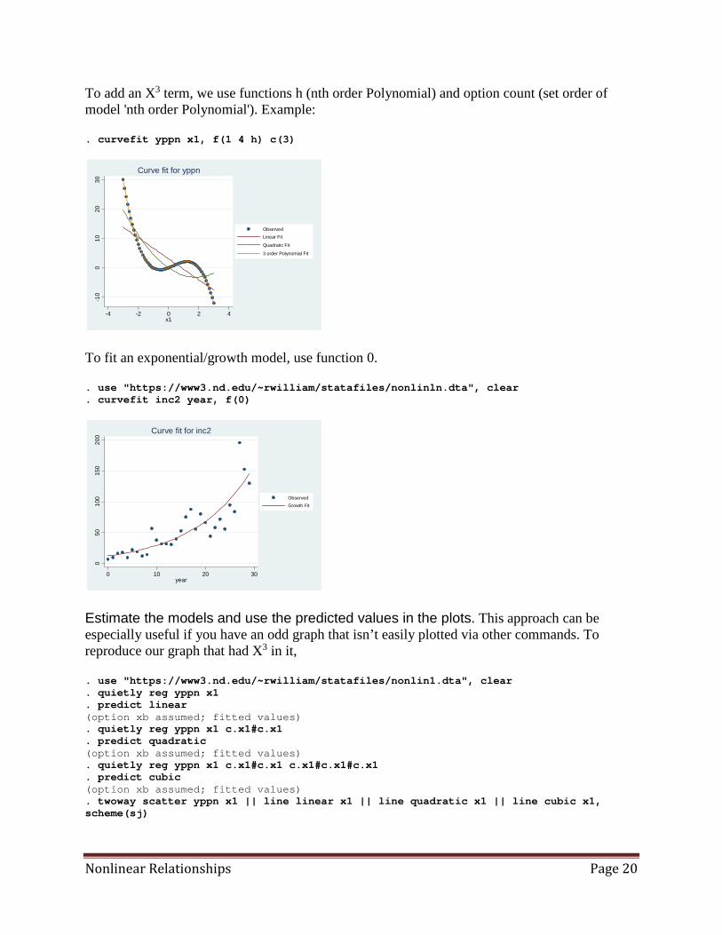
To add an X3 term, we use functions h (nth order Polynomial) and option count (set order of model 'nth order Polynomial'). Example: . curvefit yppn x1, f(1 4 h) c(3)

To fit an exponential/growth model, use function 0. . use "https://www3.nd.edu/~rwilliam/statafiles/nonlinln.dta", clear . curvefit inc2 year, f(0)

Estimate the models and use the predicted values in the plots. This approach can be especially useful if you have an odd graph that isn’t easily plotted via other commands. To reproduce our graph that had X3 in it, . use "https://www3.nd.edu/~rwilliam/statafiles/nonlin1.dta", clear . quietly reg yppn x1 . predict linear (option xb assumed; fitted values) . quietly reg yppn x1 c.x1#c.x1 . predict quadratic (option xb assumed; fitted values) . quietly reg yppn x1 c.x1#c.x1 c.x1#c.x1#c.x1 . predict cubic (option xb assumed; fitted values) . twoway scatter yppn x1 || line linear x1 || line quadratic x1 || line cubic x1, scheme(sj)

-10

010

2030

-4 -2 0 2 4x1

ObservedLinear Fit

Quadratic Fit

3 order Polynomial Fit

Curve fit for yppn

050

100

150

200

0 10 20 30year

ObservedGrowth Fit

Curve fit for inc2


For an unusual graph like our spline functions (use the sort option if data are not already sorted by x) . use "https://www3.nd.edu/~rwilliam/statafiles/blwh.dta", clear . mkspline educ1 12 educ2 = educ, marginal . reg income educ1 educ2 Source | SS df MS Number of obs = 500 -------------+------------------------------ F( 2, 497) = 618.37 Model | 28662.6998 2 14331.3499 Prob > F = 0.0000 Residual | 11518.5495 497 23.1761559 R-squared = 0.7133 -------------+------------------------------ Adj R-squared = 0.7122 Total | 40181.2493 499 80.5235456 Root MSE = 4.8142 ------------------------------------------------------------------------------ income | Coef. Std. Err. t P>|t| [95% Conf. Interval] -------------+---------------------------------------------------------------- educ1 | .9064348 .1097101 8.26 0.000 .690882 1.121988 educ2 | 1.599544 .1652037 9.68 0.000 1.274961 1.924128 _cons | 12.4063 1.167048 10.63 0.000 10.11335 14.69926 ------------------------------------------------------------------------------ . predict spline (option xb assumed; fitted values) . scatter income educ || line spline educ, sort scheme(sj)

-10

010

2030

-4 -2 0 2 4x1

yppn Fitted valuesFitted values Fitted values

010

2030

4050

0 5 10 15 20educ



Appendix B (Optional): The underlying math for piecewise regression.

The piecewise regression model can be written as

E Y X X structural break value Breakdummy( ) [( _ _ ) * ]= + + −α β β1 1 2 1

where breakdummy = 1 if X1 is greater than the structural break value, 0 otherwise. Note that the main effect of breakdummy is NOT included in the model; this implies that the intercept is the same both before and after the structural break.

So, in the case of education, the structural break value would be 12. Those with 12 years of education or less would be coded 0 on the dummy variable (and the interaction), and those with more than 12 years of education would be coded 1 on the dummy. On the interaction term, their value would be [years of education - 12].

The switching regression model can be written as

E Y X Breakdummy X structural break value Breakdummy( ) [( _ _ ) * ]= + + + −α β β β1 1 2 3 1

Both of the above correspond to the coding used by the marginal option of Stata’s mkspline command. As noted in the Stata example, you can reparameterize these depending on whether you’d rather have the coefficients represent the slope of the interval or the change in the slope from the preceding interval.

A listing of the first 20 cases in the data set makes clear how Stata has computed the variables: . list educ educ1 educ2 educ3 educ4 in 1/20 +--------------------------------------+ | educ educ1 educ2 educ3 educ4 | |--------------------------------------| 1. | 2 2 0 2 0 | 2. | 4 4 0 4 0 | 3. | 8 8 0 8 0 | 4. | 8 8 0 8 0 | 5. | 8 8 0 8 0 | |--------------------------------------| 6. | 10 10 0 10 0 | 7. | 12 12 0 12 0 | 8. | 12 12 0 12 0 | 9. | 12 12 0 12 0 | 10. | 12 12 0 12 0 | |--------------------------------------| 11. | 12 12 0 12 0 | 12. | 13 13 1 12 1 | 13. | 14 14 2 12 2 | 14. | 14 14 2 12 2 | 15. | 15 15 3 12 3 | |--------------------------------------| 16. | 15 15 3 12 3 | 17. | 16 16 4 12 4 | 18. | 16 16 4 12 4 | 19. | 17 17 5 12 5 | 20. | 21 21 9 12 9 | +--------------------------------------+


As we see, when the marginal parameter is specified, educ1 = educ, while educ2 = max(0, educ – 12). Hence, the slope for educ2 shows you the difference in effects between the first 12 years of education and any later years. When the marginal parameter is not specified, educ3 = min(educ, 12) and educ4 = max(0, educ – 12). Hence, the slope for educ4 shows you the effect for each additional year of education after year 12.

nonlinear relationships - university of notre damerwilliam/stats2/l61.pdf · and the relationship...

Documents