Dep

t. of M

athem

atical Info

rmatio

n Tech

nolo

gy

Nonlinear Multiobjective

Optimization

Jussi Hakanen, Markus Hartikainen &

Karthik Sindhya

Dept. of Mathematical Information

Technology, University of Jyväskylä,

Finland

Dep

t. of M

athem

atical Info

rmatio

n Tech

nolo

gy

Syllabus

http://users.jyu.fi/~jhaka/uppsala/syllabus.p

df

Dep

t. of M

athem

atical Info

rmatio

n Tech

nolo

gy

Where we come from?

Jyväskylä

University of Jyväskylä

Dept. of Mathematical Information

Technology

Industrial Optimization Group

January 23-27, 2012 Dagstuhl Seminar on Learning in

Multiobjective Optimization

Dep

t. of M

athem

atical Info

rmatio

n Tech

nolo

gy

A quick look at single objective

optimization

Jussi Hakanen

jussi.hakanen@jyu.fi

Dep

t. of M

athem

atical Info

rmatio

n Tech

nolo

gy

Contents

Introduction to single objective optimization

What is optimization?

Examples of optimization problems

Elements of an optimization problem

Optimality conditions

Solving an optimization problem

Optimization software

Dep

t. of M

athem

atical Info

rmatio

n Tech

nolo

gy

What is optimization?

”Scientific approach to decision making” –

Prof. Saul I. Gass

Searching for the best solution with respect

to given constraints

Enables systematic search of the best

solution (cf. trial and error)

Dep

t. of M

athem

atical Info

rmatio

n Tech

nolo

gy

Examples of practical optimization

Process design and optimization

Optimal shape design

Portfolio optimization

Route optimization in logistics

Supply chain management

etc.

Dep

t. of M

athem

atical Info

rmatio

n Tech

nolo

gy

Optimization problem

Objective function (cost function) = measure for the goodness of the solution

Variables (decision, design, ...) = values change the solution

Constraints (equality, inequality) = define feasible solutions

Feasible region = all the constraints are satisfied

Parameters = values don’t change during optimization (cf. variables)

Dep

t. of M

athem

atical Info

rmatio

n Tech

nolo

gy

Mathematical formulation

• Feasible region

• Optimality: find 𝑥∗ ∈ 𝑆 such that 𝑓 𝑥∗ ≤ 𝑓 𝑥 ∀ 𝑥 ∈ 𝑆

• Note: solutions of the optimization problems max 𝑓(𝑥) and min−𝑓(𝑥) are the same

Dep

t. of M

athem

atical Info

rmatio

n Tech

nolo

gy

Example1: mixing problem

Refinery produces 3 types of gasoline by mixing 3 different grude oil. Each grude oil can be purchased maximum of 5000 barrels per day. Let us assume that octane values and lead concentrations behave linearly in mixing. Refining costs are 4$ per barrel and the capacity of the refinery is 14000 barrels per day. Demand of gasoline can be increased by advertizing (demand grows 10 barrels per day for each $ used for advertizing).

Determine the production quantities of each type of gasoline, mixing ratios of different grude oil and the advertizing budget so that the daily profit is maximized.

Dep

t. of M

athem

atical Info

rmatio

n Tech

nolo

gy

Mixing problem

Gasoline1 Gasoline2 Gasoline3

Sale price 70 60 50

Lower limit for octane 10 8 6

Upper limit for lead 0.01 0.02 0.01

Demand 3000 2000 1000

Refining costs 4 4 4

Grude oil 1 Grude oil 2 Grude oil3

Purchase price 45 35 25

Octane value 12 6 8

Lead concentration 0.005 0.02 0.03

Availability 5000 5000 5000

Dep

t. of M

athem

atical Info

rmatio

n Tech

nolo

gy

Mixing problem

Variables:

– 𝑥𝑖𝑗 = amount of grude oil 𝑖 used for producing gasoline 𝑗

– 𝑦𝑗 = the amount of money used for advertizing gasoline 𝑗 Net income:

– 𝑥11: 70 − 45 − 4 = 21

– 𝑥12: 60 − 45 − 4 = 11

– 𝑥13: 50 − 45 − 4 = 1

– 𝑥21: 70 − 35 − 4 = 31

– 𝑥22: 60 − 35 − 4 = 21

– 𝑥23: 50 − 35 − 4 = 11

– 𝑥31: 70 − 25 − 4 = 41

– 𝑥32: 60 − 25 − 4 = 31

– 𝑥33: 50 − 25 − 4 = 21

Dep

t. of M

athem

atical Info

rmatio

n Tech

nolo

gy

Mixing problem

Objective function:

– max 21 𝑥11 + 11 𝑥12 + 𝑥13 + 31𝑥21 +21𝑥22 + 11𝑥23 + 41𝑥31 + 31𝑥32 +21𝑥33 − 𝑦1 − 𝑦2 − 𝑦3

Nonnegativity:

– 𝑥𝑖𝑗 ≥ 0 ∀ 𝑖, 𝑗 𝑎𝑛𝑑 𝑦𝑗 ≥ 0 ∀ 𝑗

Capacity:

– 𝑥𝑖𝑗3𝑗=1

3𝑖=1 ≤ 14000

Dep

t. of M

athem

atical Info

rmatio

n Tech

nolo

gy

Mixing problem

Demands:

– Gasoline 1: 𝑥11 + 𝑥21 + 𝑥31 = 3000 + 10𝑦1

– Gasoline 2: 𝑥12 + 𝑥22 + 𝑥32 = 2000 + 10𝑦2

– Gasoline 3: 𝑥13 + 𝑥23 + 𝑥33 = 1000 + 10𝑦3

Availabilities:

– Grude oil 1: 𝑥11 + 𝑥21 + 𝑥31 ≤ 5000

– Grude oil 2: 𝑥12 + 𝑥22 + 𝑥32 ≤ 5000

– Grude oil 3: 𝑥13 + 𝑥23 + 𝑥33 ≤ 5000

Dep

t. of M

athem

atical Info

rmatio

n Tech

nolo

gy

Mixing problem

Octane values:

– Gasoline 1: 12𝑥11+ 6𝑥21+8𝑥31𝑥11+ 𝑥21+𝑥31

≥ 10

– Gasoline 2: 12𝑥12+ 6𝑥22+8𝑥32𝑥12+ 𝑥22+𝑥32

≥ 8

– Gasoline 3: 12𝑥13+ 6𝑥23+8𝑥33𝑥13+ 𝑥23+𝑥33

≥ 6

Lead concentrations:

– Gasoline 1: 0.005𝑥11+ 0.02𝑥21+0.03𝑥31

𝑥11+ 𝑥21+𝑥31 ≤ 0.01

– Gasoline 2: 0.005𝑥12+ 0.02𝑥22+0.03𝑥32

𝑥12+ 𝑥22+𝑥32 ≤ 0.02

– Gasoline 3: 0.005𝑥13+ 0.02𝑥23+0.03𝑥33

𝑥13+ 𝑥23+𝑥33 ≤ 0.01

Dep

t. of M

athem

atical Info

rmatio

n Tech

nolo

gy

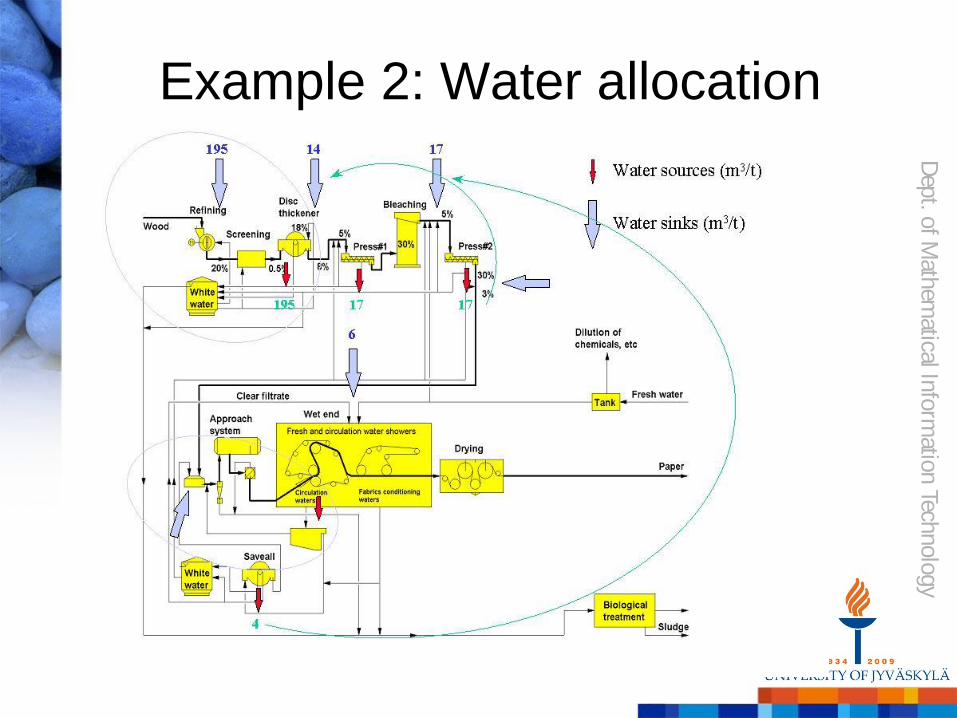
Example 2: Water allocation

Dep

t. of M

athem

atical Info

rmatio

n Tech

nolo

gy

Water allocation

Papermaking process consumes lots of water

Water can be circulated and reused in different parts of the process as long as it remains fresh enough

Fresh water costs

The aim is to minimize the amount of fresh water required by the process

How to formulate the optimization problem?

Dep

t. of M

athem

atical Info

rmatio

n Tech

nolo

gy

Water allocation

Objective function: minimize the amount of fresh water used

Constraints:

– water used should be fresh enough

– Energy and mass balances between the different unit processes (requires a process model)

Can not (usually) be formulated explicitly but requires e.g. the use of a process simulation software

Dep

t. of M

athem

atical Info

rmatio

n Tech

nolo

gy

Different types of optimization

problems

Linear = all functions are linear

Nonlinear = at least one function is nonlinear

Continuous = variables real-valued

Discrete = only finite (or countable) number of

possible values for the variables

Stochastic = problem contains uncertainties

Multiobjective = multiple objective functions

Dep

t. of M

athem

atical Info

rmatio

n Tech

nolo

gy

Different types of optimization

problems

Unconstraint = all values of the variables

are feasible

Box constraints = variables have upper and

lower bounds

Linear constraints = feasible region is

convex polyhedron

Nonlinear constraints = feasible region can

be anything

Dep

t. of M

athem

atical Info

rmatio

n Tech

nolo

gy

Local vs. global optima

-5 -4 -3 -2 -1 0 1 2

-1.5

-1

-0.5

0

0.5

1

1.5

2

minimize sin(x2+x)+cos(3x) -5≤x≤2

global minimum

local minima

Adopted from Prof. Janos D. Pinter

Dep

t. of M

athem

atical Info

rmatio

n Tech

nolo

gy

Local vs. global optima

-4

-2

0

2

4

-4

-2

0

2

-1

0

1

2

-4

-2

0

2

4

Only two variables… → curse of dimensionality

Adopted from Prof. Janos D. Pinter

Dep

t. of M

athem

atical Info

rmatio

n Tech

nolo

gy

How to find optimal solutions?

Trial and error → widely used in practice, not

efficient and high possibility to miss good

solutions

Better to use a systematic way to find optimal

solution

Typically we know only

– function value(s) at the current trial point

– possibly gradients at the current trial point

How can we know when an optimal solution

has been reached?

Dep

t. of M

athem

atical Info

rmatio

n Tech

nolo

gy

Optimality conditions

How can we know that a solution is optimal?

One way is to utilize optimality conditions

Necessary optimality conditions = conditions

that an optimal solution has to satisfy (does

not guarantee optimality)

Sufficient optimality conditions = conditions

that guarantee optimality when satisfied

1. order conditions (1. order derivatives) and 2.

order conditions (2. order derivatives)

Dep

t. of M

athem

atical Info

rmatio

n Tech

nolo

gy

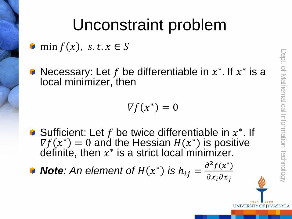
Unconstraint problem

min 𝑓 𝑥 , 𝑠. 𝑡. 𝑥 ∈ 𝑆

Necessary: Let 𝑓 be differentiable in 𝑥∗. If 𝑥∗ is a local minimizer, then

𝛻𝑓 𝑥∗ = 0

Sufficient: Let 𝑓 be twice differentiable in 𝑥∗. If 𝛻𝑓 𝑥∗ = 0 and the Hessian 𝐻(𝑥∗) is positive definite, then 𝑥∗ is a strict local minimizer.

Note: An element of 𝐻 𝑥∗ is ℎ𝑖𝑗 =𝜕2𝑓(𝑥∗)

𝜕𝑥𝑖𝜕𝑥𝑗

Dep

t. of M

athem

atical Info

rmatio

n Tech

nolo

gy

Info: Definite Matrices

A symmetric 𝑛 × 𝑛 matrix 𝐻 is positive

semidefinite if ∀ 𝑥 ∈ ℝ𝑛

𝑥𝑇𝐻𝑥 ≥ 0.

A symmetric 𝑛 × 𝑛 matrix 𝐻 is positive

definite if

𝑥𝑇𝐻𝑥 > 0 ∀ 0 ≠ 𝑥 ∈ ℝ𝑛.

Dep

t. of M

athem

atical Info

rmatio

n Tech

nolo

gy

Example of optimality conditions

-5 -4 -3 -2 -1 0 1 2

-1.5

-1

-0.5

0

0.5

1

1.5

2

minimize sin(x2+x)+cos(3x)

satisfies both necessary and sufficient conditions

satisfies only necessary conditions

Adopted from Prof. Janos D. Pinter

Dep

t. of M

athem

atical Info

rmatio

n Tech

nolo

gy

Unconstraint problem

Adopted from Prof. L.T. Biegler (Carnegie Mellon

University)

Dep

t. of M

athem

atical Info

rmatio

n Tech

nolo

gy

Inequality constraints

Adopted from Prof. L.T. Biegler (Carnegie Mellon

University)

Dep

t. of M

athem

atical Info

rmatio

n Tech

nolo

gy

Inequality and equality constraints

Adopted from Prof. L.T. Biegler (Carnegie Mellon

University)

Dep

t. of M

athem

atical Info

rmatio

n Tech

nolo

gy

Optimality conditions: necessary

Dep

t. of M

athem

atical Info

rmatio

n Tech

nolo

gy

Optimality conditions: sufficient

Dep

t. of M

athem

atical Info

rmatio

n Tech

nolo

gy

Solving an optimization problem

Find optimal values 𝑥∗ for the variables

Problems that can be solved analytically

min 𝑥2, 𝑤ℎ𝑒𝑛 𝑥 ≥ 3 → 𝑥∗ = 3

Usually impossible to solve analytically

Must be solved numerically →

approximation of the solution

Dep

t. of M

athem

atical Info

rmatio

n Tech

nolo

gy

Numerical solution

Modelling → mathematical model of the

problem

Numerical methods → numerical simulation

model for the mathematical model

Optimization method → solve the problem

utilizing the numerical simulation model

SO

modelling → simulation → optimization

Dep

t. of M

athem

atical Info

rmatio

n Tech

nolo

gy

Optimization method

Algorithm: a mathematical description 1. Choose a stopping parameter 𝜀 > 0, starting point 𝑥1 and a

symmetric positive definite 𝑛 × 𝑛 matrix 𝐷1(e.g. 𝐷1 = 𝐼). Set 𝑦1 = 𝑥1 and ℎ = 𝑗 = 1.

2. If 𝛻𝑓(𝑦𝑗) < 𝜀, stop. Otherwise, set 𝑑𝑗 = −𝐷𝛻𝑓(𝑦𝑗). Let 𝜆𝑗 be a solution of

min 𝑓(𝑦𝑗 + 𝜆𝑑𝑗), s.t. 𝜆 ≥ 0.

Set 𝑦𝑗+1 = 𝑦𝑗 + 𝜆𝑗𝑑𝑗. If 𝑗 = 𝑛, set 𝑦1 = 𝑥ℎ+1 = 𝑦𝑛+1, ℎ = ℎ + 1, 𝑗 = 1

and repeat (2).

3. Compute 𝐷𝑗+1. Set 𝑗 = 𝑗 + 1 and go to (2).

Method: numerical methods included

Software: a method implemented as a computer programme

Dep

t. of M

athem

atical Info

rmatio

n Tech

nolo

gy

Local optimization methods

Find a (closest) local optimum

Fast

Usually utilize derivatives

Mathematical convergence

For example

– Direct search methods (pattern search, Hooke & Jeeves, Nelder & Mead, …)

– Gradient based methods (steepest descent, Newton’s method, quasi-Newton method, conjugate gradient, SQP, interior point methods…)

Dep

t. of M

athem

atical Info

rmatio

n Tech

nolo

gy

Global optimization methods

Try to get as close to global optimum as

possible

No mathematical convergence

Do not assume much of the problem

Slow, use lots of function evaluations

Heuristic, contain randomness

Most well known are evolutionary methods

– based on improving a population of

solutions at a time instead of a single

solution

Dep

t. of M

athem

atical Info

rmatio

n Tech

nolo

gy

Hybrid methods

Combination of global and local methods

Try to combine the benefits of both

– rough estimate with a global method,

fine tune with a local method

Challenge: how the methods should be

combined?

– e.g. when to switch from global to local?

(speed vs. accuracy)

Dep

t. of M

athem

atical Info

rmatio

n Tech

nolo

gy

On selecting a software

Lots of software available (also open

source)

Decision Tree for Optimization Software,

http://plato.asu.edu/guide.html

NEOS Optimization Software Guide,

http://www.neos-guide.org/Optimization-

Guide

Dep

t. of M

athem

atical Info

rmatio

n Tech

nolo

gy

Optimization platforms

AIMMS, http://www.aimms.com/

AMPL, http://www.ampl.com/

GAMS, http://www.gams.com/

Matlab,

http://www.mathworks.com/products/matlab

MPL, http://www.maximalsoftware.com/

Dep

t. of M

athem

atical Info

rmatio

n Tech

nolo

gy

Matlab example (by yourself)

Solve the mixing problem related to oil

refinery introduced earlier with Matlab

Matlab Optimization toolbox

Routine linprog is an optimization method

for linear problems

Dep

t. of M

athem

atical Info

rmatio

n Tech

nolo

gy

Examples of optimization

literature

P.E. Gill et al., Practical Optimization, 1981

M.S. Bazaraa et al., Nonlinear Programming: Theory and Algorithms, 1993

D.P. Bertsekas, Nonlinear Programming, 1995

S.S. Rao, Engineering Optimization: Theory and Practice, 1996

J. Nocedal, Numerical Optimization, 1999

A.R. Conn et al., Introduction to Derivative-Free Optimization, 2009

M. Hinze et al., Optimization with PDE Constraints, 2009

L.T. Biegler, Nonlinear Programming – Concepts, Algorithms, and Applications to Chemical Processes, 2010

Dep

t. of M

athem

atical Info

rmatio

n Tech

nolo

gy

Journals in optimization Applied Mathematics and Optimization

Computational Optimization and Applications

European Journal of Operational Research

Decision Support Systems

Journal of Global Optimization

Journal of Multi-Criteria Decision Analysis

Journal of Optimization Theory and Applications

Mathematical Programming

Omega

Operations Research

Optimization Letters

Optimization Methods and Software

Optimization

SIAM Journal on Control and Optimization

SIAM Journal on Optimization

Structural and Multidisciplinary Optimization

…

Dep

t. of M

athem

atical Info

rmatio

n Tech

nolo

gy

Examples of journals in

application areas

AIChE Journal

American Institute of Aeronautics and Astronautics

Applied Thermal Engineering

Computers & Chemical Engineering

Engineering Optimization

Engineering with Computers

Environmental Modelling & Software

Industrial & Engineering Chemistry Research

Journal of Environmental Engineering and Science

Optimization and Engineering

Water Science and Technology

…