nonlinear modeling of an electric submersible pump ... · pdf filenonlinear modeling of an...

International Journal of Scientific Research and Innovative Technology ISSN: 2313-3759 Vol. 3 No. 4; April 2016

27

Nonlinear Modeling of an Electric Submersible Pump Operating with Multiphase Flow by SVMr and Genetic Algorithms

BY

G. E. CASTAÑEDA JIMENEZ1, 2, D. M. MARTINEZ RICARDO1, 2, AND J. VAQUEIRO FERREIRA1

1 Department of Computational Mechanics, UNICAMP-University of Campinas, Brazil

2 Students-Agreement Graduate - PEC-PG, CAPES / CNPq – Brazil

ABSTRACT

In the oil industry, it is common to use submersible electric pumps (ESP) operating with multiphase fluid flow

"gas-liquid". The presence of large amounts of gas in the pump generates instabilities and degradation in

performance of the pump. In this paper it is presented a method to create a nonlinear model, which

interpolates the behavior of an ESP operating with multiphase fluid flow, using artificial intelligence from

experimental data.The method is based on support vector machines for regression (SVMr), which is a robust

tools capable of solving nonlinear and high dimensional problems. Once the SVMr have internal parameters

that influence the performance of it, this paper used a genetic algorithm as optimizer of the SVMr parameters

to reach a good solution to the problem. The results obtained with SVMr and the data set shows that it is

possible to obtain representative models with artificial intelligence and a limited number of training data.

Keywords: submersible electric pumps, support vector machines for regression, genetic algorithm, machine

learning.


28

1 Introduction The submersible electric pump (ESP) is a method widely used for artificial lift, which comprises a centrifugal

pump with multiples stages normally installed at the end of the column of production within the oil well. The

produced fluid in the well is sometimes a liquid gas mixture. The presence of gas causes changes in the

properties of the pumped fluid, such as change in density, viscosity and the presence of a gas phase, which in

turn can cause severe impacts on the performance of the ESP( MONTE, 2011)(G DUTRA, 2007)(GAMBOA

& PRADO , 2007).

Figure 1 shows the performance curve of a pump operating with gas-liquid fluid flow, with different

percentages of gas in which∆� is the pressure differential between the output and input of ESP and � is the

total fluid flow, ie, flow of liquid fluid plus the airflow fluid.Curve (1) represents the operation of the pump

with a single phase fluid flow, that is, single or two phase liquid with a very small amount of gas. The curve

(2) represents the behavior of the pump with a small increase in the amount of gas, as shown only exhibits a

small loss in lifting capacity, since the amount of gas is still low and the fluid flow has a behavior

homogeneous, i.e., the bubbles are dispersed in the liquid. Curve (3) shows a characteristic curve when the

amount of gas in the mixture is greater, showing a peak of the curve. This peak is known as the point of

"surging", characterized by a considerable decrease in its pumping capacity. Under these conditions the flow is

no longer homogeneous, i.e., liquid and gas in the multiphase mixture are flowing separately. When there is a

large presence of gas in the flow, the performance curve presents new instabilities shown on curved (4) which

has three different ranges; Range (a) shows a stable operation, that is, the mixture is homogeneous; Range (b)

starts at the point of surging, showing a loss in pressure and pumping capacity; Range (c) shoes the presence

of large amounts of free gas at low flow rates that may cause clogging in the surface available for flow in the

pump rotor, causing the flow rate to be zero, a phenomenon known as “gas locking“.

The use of ESP operating with gas-liquid multiphase flow is common in the oil industry, for this reason there

is great interest to know the performance of pumps in wells. Currently researches focuses on the empirical

study of the behavior of pumps working with multiphase fluid flow, and it has been criticalto understand and

provide information on the actual behavior of the ESP operating with liquid-gas fluidflows in the wells.Exists

a great difficulty for obtaining mathematical models representing the performance of the pumps in the three

ranges shown in Figure 1with physical laws, so in this work is presented ageneration of a non-parametric

model using artificial intelligence and experimental data as a basis for the training of the algorithm.

2 Support Vector Machine for Regression (SVMr) The support vector machine (SVMr) are machine learning algorithms for supervised classification and

regression problems developed by Vladimir Vapnik(VAPNIK & STEVEN, 1996)( HONG & YONGMEI,

2013).

In this paper is used for regression, where you have a set of training data ��, �� ,�,…,�, where each �� ∈ �� represents a sample of the input data and each � ∈ �an object. The aim of the SVMr, is to find a

function��representing the objectives�y� withaccuracy ϵ, which means estimate the regression coefficients

of ��with the requirements given (STOEAN, DUMITRESCU, PREUSS, & STOEAN, 2006)(SMOLA &

SCHOLKOPF, 2004).

Suppose you have a linear regression model that can adjust the training data as shown in Figure 2,

consequently the function ��has the form: �� = ⟨�, �⟩ + � ( 1 )

in which� ∈ �� is the slope of the regression plane and � ∈ �is the -intercept of the surface.


29

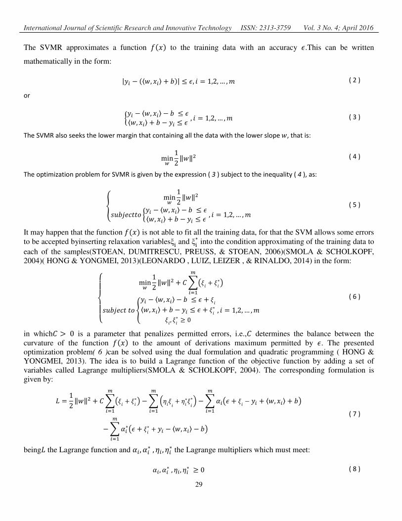
The SVMR approximates a function �� to the training data with an accuracy �.This can be written

mathematically in the form:

|� − �⟨�, ��⟩ + �| ≤ �, " = 1,2,… ,% ( 2 )

or

&� − ⟨�, ��⟩ − � ≤ �⟨�, ��⟩ + � − � ≤ � , " = 1,2,… ,%' ( 3 )

The SVMR also seeks the lower margin that containing all the data with the lower slope �, that is:

min+ 12 ‖�‖� ( 4 )

The optimization problem for SVMR is given by the expression ( 3 ) subject to the inequality ( 4 ), as:

- min+ 12 ‖�‖�./�012334 &� − ⟨�, ��⟩ − � ≤ �⟨�, ��⟩ + � − � ≤ � , " = 1,2,… ,%'' ( 5 )

It may happen that the function �� is not able to fit all the training data, for that the SVM allows some errors

to be accepted byinserting relaxation variablesξ� and ξ�∗ into the condition approximating of the training data to

each of the samples(STOEAN, DUMITRESCU, PREUSS, & STOEAN, 2006)(SMOLA & SCHOLKOPF,

2004)( HONG & YONGMEI, 2013)(LEONARDO , LUIZ, LEIZER , & RINALDO, 2014) in the form:

6778779 min+ 12 ‖�‖� + :;<=" + ="∗>�

�� ./�012334 ?� − ⟨�, ��⟩ − � ≤ � + ="⟨�, ��⟩ + � − � ≤ � + ="∗=", ="∗ ≥ 0 , " = 1,2, … ,%'' ( 6 )

in which: > 0 is a parameter that penalizes permitted errors, i.e.,: determines the balance between the

curvature of the function �� to the amount of derivations maximum permitted by �. The presented

optimization problem( 6 )can be solved using the dual formulation and quadratic programming ( HONG &

YONGMEI, 2013). The idea is to build a Lagrange function of the objective function by adding a set of

variables called Lagrange multipliers(SMOLA & SCHOLKOPF, 2004). The corresponding formulation is

given by:

C = 12‖�‖� + :;<=" + ="∗>�� −;DE"=" + E"∗="∗F�

�� −;G�<� + =" − � + ⟨�, ��⟩ + �>��

−;G�∗<� + ="∗ + � − ⟨�, ��⟩ − �>��

( 7 )

beingC the Lagrange function and G�, G�∗, E� , E�∗ the Lagrange multipliers which must meet:

G�, G�∗, E�, E�∗ ≥ 0 ( 8 )


30

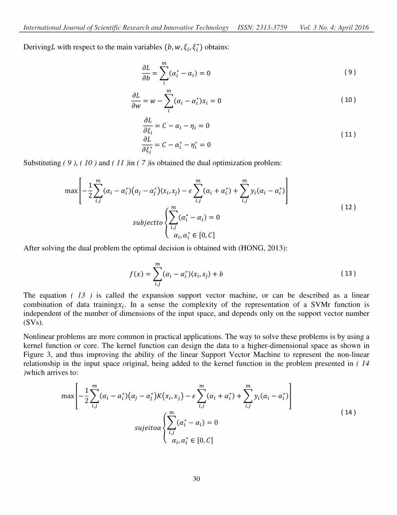
DerivingC with respect to the main variables ��, �, =� , =�∗ obtains:

HCH� =;�G�∗ − G�� = 0 ( 9 )

HCH� = � −;�G� − G�∗�� = 0 ( 10 )

HCH=� = : − G� − E� = 0HCH=�∗ = : − G�∗ − E�∗ = 0 ( 11 )

Substituting ( 9 ), ( 10 ) and ( 11 )in ( 7 )is obtained the dual optimization problem:

max K−12;�G� − G�∗<GL − GL∗>⟨��, �L⟩��,L − �;�G� + G�∗�

�,L +;��G� − G�∗��,L M

./�012334 -;�G�∗ − G��,L = 0G� , G�∗ ∈ N0, :O

' ( 12 )

After solving the dual problem the optimal decision is obtained with (HONG, 2013):

�� =;�G� − G�∗⟨��, �L⟩ + ��,L ( 13 )

The equation ( 13 ) is called the expansion support vector machine, or can be described as a linear

combination of data training��. In a sense the complexity of the representation of a SVMr function is

independent of the number of dimensions of the input space, and depends only on the support vector number

(SVs).

Nonlinear problems are more common in practical applications. The way to solve these problems is by using a

kernel function or core. The kernel function can design the data to a higher-dimensional space as shown in

Figure 3, and thus improving the ability of the linear Support Vector Machine to represent the non-linear

relationship in the input space original, being added to the kernel function in the problem presented in ( 14

)which arrives to:

max K−12;�G� − G�∗<GL − GL∗>P<�� , �L>��,L − �;�G� + G�∗�

�,L +;��G� − G�∗��,L M

./01"34Q -;�G�∗ − G��,L = 0G�, G�∗ ∈ N0, :O

' ( 14 )


31

beingP<�� , �L> the function kernel. After solving the problem presented in ( 14 )the optimal decision function

with the kernel is given by:

�� =;�G� − G�∗P<�� , �L> + ��,L ( 15 )

The larger the size of the space description, the better the kernel will provide a greater probability of obtaining

a hyperplane. By turning the input space into a higher space (theoretically of infinite dimension), it is possible

to obtain a separation of classes by hyperplanes ( HONG & YONGMEI, 2013).

3 SVMr Parameters Optimization using Genetic Algorithms Genetic algorithms (GA) developed by (HOLLAND J. E., 1975)(HOLLAND J. H., 1992), are adaptive

methods that can be used to solve search and optimization problems. They are based on the genetic process of

living beings. The process of evolution is based on nature, is the natural principles and the survival of the

fittest. This optimization strategy can be used for the search of hidden parameters of SVMr in order to

improve its performance(HUA & YONG XIN, 2009)(QILONG, GANLIN, XIUSHENG, & ZINING,

2009)(CAO, ZHOU, LI, WU, & LIU, 2008). Figure 4 shows the flow diagram of a simplex genetic algorithm

in which are shown the most important aspects that will be explained for the case of optimization of SVMr

parameters.

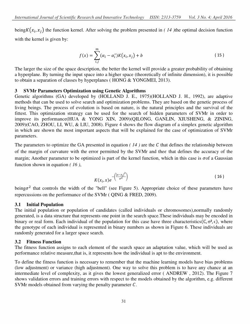
The parameters to optimize the GA presented in equation ( 14 ) are the : that defines the relationship between

of the margin of curvature with the error permitted by the SVMr and the� that defines the accuracy of the

margin; Another parameter to be optimized is part of the kernel function, which in this case is Rof a Gaussian

function shown in equation ( 16 ),

P�� , �1STUVWVXUYZY [

( 16 )

beingR� that controls the width of the "bell" (see Figure 5). Appropriate choice of these parameters have

repercussions on the performance of the SVMr ( QING & FRED, 2009).

3.1 Initial Population The initial population or population of candidates (called individuals or chromosomes),normally randomly

generated, is a data structure that represents one point in the search space.These individuals may be encoded in

binary or real form. Each individual of the population for this case have three characteristics�C, σ², ϵ, where

the genotype of each individual is represented in binary numbers as shown in Figure 6. These individuals are

randomly generated for a larger space search.

3.2 Fitness Function The fitness function assigns to each element of the search space an adaptation value, which will be used as

performance relative measure,that is, it represents how the individual is apt to the environment.

To define the fitness function is necessary to remember that the machine learning models have bias problems

(low adjustment) or variance (high adjustment). One way to solve this problem is to have any chance at an

intermediate level of complexity, as it gives the lowest generalized error ( ANDREW , 2012). The Figure 7

shows validation errors and training errors with respect to the models obtained by the algorithm, e.g. different

SVMr models obtained from varying the penalty parameter :.


32

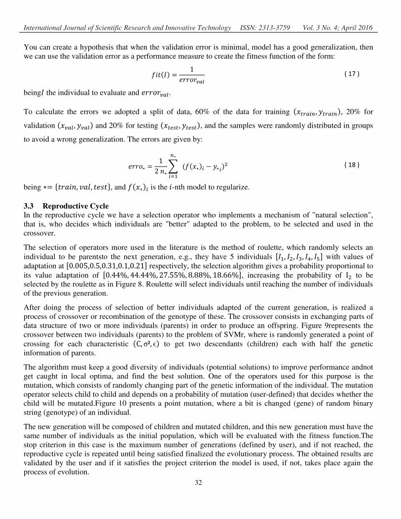
You can create a hypothesis that when the validation error is minimal, model has a good generalization, then

we can use the validation error as a performance measure to create the fitness function of the form:

�"3�] = 11^^4 _̂à ( 17 )

being] the individual to evaluate and 1^^4 _̂à. To calculate the errors we adopted a split of data, 60% of the data for training ��bc`��, bc`��, 20% for

validation ��_à, _à and 20% for testing ��bdeb, bdeb, and the samples were randomly distributed in groups

to avoid a wrong generalization. The errors are given by:

1^^4∗ = 12f∗;��∗� − ∗��∗�� ( 18 )

being ∗= �3^Q"f, gQh, 31.3�, and ��∗� is the "-nth model to regularize.

3.3 Reproductive Cycle In the reproductive cycle we have a selection operator who implements a mechanism of "natural selection",

that is, who decides which individuals are "better" adapted to the problem, to be selected and used in the

crossover.

The selection of operators more used in the literature is the method of roulette, which randomly selects an

individual to be parentsto the next generation, e.g., they have 5 individuals N] , ]�, ]i, ]j, ]kO with values of

adaptation at N0.005,0.5,0.31,0.1,0.21O respectively, the selection algorithm gives a probability proportional to

its value adaptation of N0.44%, 44.44%, 27.55%, 8.88%, 18.66%O, increasing the probability of I� to be

selected by the roulette as in Figure 8. Roulette will select individuals until reaching the number of individuals

of the previous generation.

After doing the process of selection of better individuals adapted of the current generation, is realized a

process of crossover or recombination of the genotype of these. The crossover consists in exchanging parts of

data structure of two or more individuals (parents) in order to produce an offspring. Figure 9represents the

crossover between two individuals (parents) to the problem of SVMr, where is randomly generated a point of

crossing for each characteristic �C, σ², ϵ to get two descendants (children) each with half the genetic

information of parents.

The algorithm must keep a good diversity of individuals (potential solutions) to improve performance andnot

get caught in local optima, and find the best solution. One of the operators used for this purpose is the

mutation, which consists of randomly changing part of the genetic information of the individual. The mutation

operator selects child to child and depends on a probability of mutation (user-defined) that decides whether the

child will be mutated.Figure 10 presents a point mutation, where a bit is changed (gene) of random binary

string (genotype) of an individual.

The new generation will be composed of children and mutated children, and this new generation must have the

same number of individuals as the initial population, which will be evaluated with the fitness function.The

stop criterion in this case is the maximum number of generations (defined by user), and if not reached, the

reproductive cycle is repeated until being satisfied finalized the evolutionary process. The obtained results are

validated by the user and if it satisfies the project criterion the model is used, if not, takes place again the

process of evolution.


33

4 Application of the SVMr with GA for the Modeling of an ESP The ESP model in this work has the structure depicted in Figure 11 having as inputs the pressure in the suction

side of the ESP ��, the percentage of gas in the mixture �%`c, the pump rotation �uvwx and the flow of

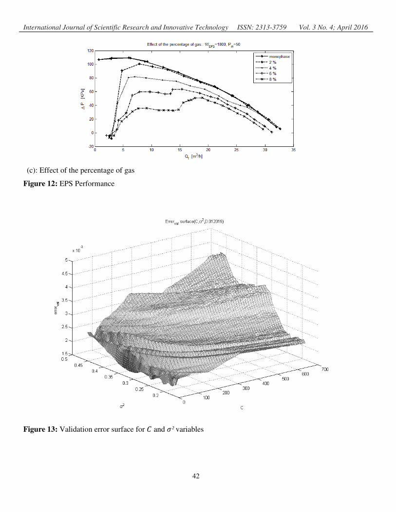
the liquid-gas mixture ��b, and as output the pressure generated by ESP ��yzb. Figure 12 shows the performance curves (flow-pressure) of the pumpoperating at different conditions, in

which in Figure 12.ashows the effect of the rotation of ESP,in Figure 12.b shows the effect of pressure input

and in Figure 12.cshowsthe effect of the percentage of gas.

As for the training process was used a data set (Data of ( MONTE, 2011)) a pump GN 7000, with operation

ranges for a pressure of �50,100,200�P�Q, rotations of�1200,1800,2400�{�|, and percentage of gas �0,2,4,6,8,10�%, thus having the flow-pressure performance curves shown in Table 1. The data set (714

samples) were randomly allocated into three groups: 60 % for training (500 samples), 20 % for validation (107

samples) and 20 % for testing (107 samples).

The input parameters in the genetic algorithm are:

• Individuals: �40,80,100� • Chromosome length: �60� bits; �20� Bits to :N2S }, 2 }O, �20� bits to σ²N2S k, 2kO and �20� bits to �N2S ~, 2�O • Crossover probability: �50�%

• Mutation probability: �20�%

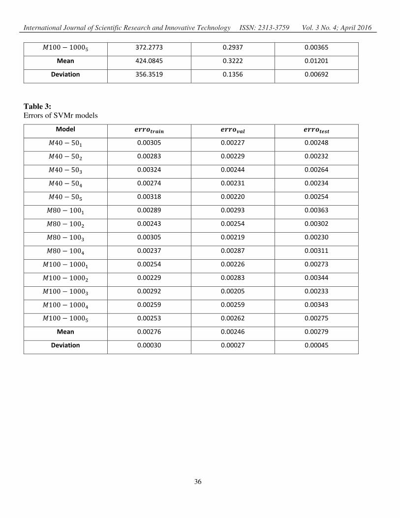
• Generations: �50,100,1000� After the training phase delivered by genetic algorithm, it is possible to see the results. Table 2 shows

parameters for the SVMr. Table 3 displays its training errors, validation and test for each model. For the

process of obtaining and optimization of SVMr models, it was used the library LIBSVM (CHANG & LIN.,

2011).

The notation used �|f�� − �� in the name of the models makes reference to the input parameters for the

genetic algorithm, being | the model, f�� the number of individuals in the population, � is a number of

generations used as a criterion for stop, and the index iis referencing the model number, e.g., the model M80 − 100� has 80 individuals in the population, the stopping criterion has 100 generations and is the second

model obtained with these input parameters for the GA.

From Table 2 and Table 3 can be seen that there is a rank of values for : and σ² that can give a good

performance in terms of minimizing the validation error. It can also be seen that the test error have low values,

i.e., the model generalizes well the data. The above results can be seen in Figure 13 where the validation error

has similar errors for different values of :and σ².

Studying the performance of each model shown in the Table 2 and Table 3, the best result having as a criterion

the model offering the best generalization, i.e.,lower test error, according to Table 3was |80 − 100i with

parameters : = 381.2881, σ� = 0.2498 and � = 0.01080, reaching a test error �0.00230, being the model

that has the lowest error validation �0.00219. 5 Conclusion In this work, it were developed nonlinear models based on SVM algorithms capable of interpolating the ESP

behavior at different points of operation (pressure, flow, speed and gas percentage) from experimental data.

These models have a good generalization, because for training phase was performed a optimization of the

hidden parameters of SVMr �C, σ², ϵ using genetic algorithms, taking into account that the GA has trouble


34

finding the global optimum since some variations in hidden parameters from SVMr show similar results,

without harming the performance of the models obtained for the ESP.

References ANDREW , N. (2012). Introduction to machine learning. In Machine learning Course.

HONG, Z., & YONGMEI, L. (2013). Bsp-based support vector regression machine parallel framework.

Computer and Information Science (ICIS), 2013 IEEE/ACIS 12th, 329-334.

MONTE, V. W. (2011). Estudo experimental de bombas de bcs operando com escoamento bifásico gás-l´

ıquido. Master’s thesis, FEM/UNICAMP.

QING, Y., & FRED, R. (2009). Parameter selection of support vector regression machine based on differential

evolution algorithm. Sixth International Conference on Fuzzy Systems and Knowledge Discovery,

IEEE, vol 2, 596-598.

CAO, L., ZHOU, S., LI, R., WU, F., & LIU, T. (2008). Application of optimizing the parameters of svm using

genetic simulated annealing algorithm. 7th World Congress on Intelligent Control and Automation.

CHANG, C. C., & LIN., C. J. (2011). Libsvm : a library for support vector machines. ACM Transactions on

Intelligent Systems and Technology, 2:27:1-27:27.

G DUTRA, L. (2007). Modelagem do escoamento monofásico em bomba centrífuga submersa operando com

fluidos viscosos. Master’s thesis FEM/UNICAMP.

GAMBOA , J. J., & PRADO , M. (2007). Multiphase performance of esp stages-part I. The University of

Tulsa, Artificial Lift Projects.

HOLLAND, J. E. (1975). Adaptation in Natural and Artificial Systems. University of Michigan Press.

HOLLAND, J. H. (1992). Adaptation in Natural and Artificial Systems. 2nd edition, The MIT Press.

HUA, L., & YONG XIN, Z. (2009). An algorithm of soft fault diagnosis for analog circuit based on the

optimized svm by ga. he Ninth International Conference on Electronic Measurement & Instruments.

LEONARDO , F., LUIZ, H. S., LEIZER , S., & RINALDO, A. (2014). Elevação de petróleo por bcs via

técnica de controle fuzzy pid. XX Congresso Brasileiro de Automática.

QILONG, Z., GANLIN, S., XIUSHENG, D., & ZINING, Z. (2009). Parameters optimization of support

vector machine based on simulated annealing and genetic algorithm. IEEE International Conference

on Robotics and Biomimetics.

SMOLA , J. S., & SCHOLKOPF, B. A. (2004). A tutorial on support vector regression. Kluwer Academic

Publishers. Manufactured in The Netherlands, Statistics and Computing 14, 199-222.

STOEAN, S., DUMITRESCU, D., PREUSS, M., & STOEAN, C. (2006). Evolutionary support vector

regression machines. Symbolic and Numeric Algorithms for Scientific Computing, 330-335.

VAPNIK, V., & STEVEN, E. (1996). Support Vector Method for Function Approximation, Regression

Estimation, and Signal Processing. Advances in Neural Information Processing Systems 9, 281--287.


35

Tables

Table 1: Performance curves employed for learning model �� %��

50P�Q

0% 2% 4% 6% 8% 10%

�� %��

50P�Q

0% 2% 4% 6% 8% 10%

100P�Q 6% 10%

200P�Q 6% 10%

�� %��

50P�Q

0% 2% 4% 6% 8% 10%

Table 2: Results of the optimization of the parameters of SVMr with AG

Model � �² � |40 − 50 600.918 0.2268 0.01396 |40 − 50� 1003.1934 0.2221 0.00897 |40 − 50i 740.1055 0.2000 0.01750 |40 − 50j 271.0596 0.2963 0.01118 |40 − 50k 967.7246 0.1960 0.01362 |80 − 100 924.9834 0.2290 0.03170 |80 − 100� 138.8623 0.3723 0.01351 |80 − 100i 381.2881 0.2498 0.01080 |80 − 100j 136.3564 0.3840 0.00203 |100 − 1000 138.3994 0.3404 0.01085 |100 − 1000� 38.8457 0.5362 0.00834 |100 − 1000i 212.748 0.2946 0.01079 |100 − 1000j 10.4219 0.6696 0.01126


36

|100 − 1000k 372.2773 0.2937 0.00365

Mean 424.0845 0.3222 0.01201

Deviation 356.3519 0.1356 0.00692

Table 3: Errors of SVMr models

Model �� |40 − 50 0.00305 0.00227 0.00248 |40 − 50� 0.00283 0.00229 0.00232 |40 − 50i 0.00324 0.00244 0.00264 |40 − 50j 0.00274 0.00231 0.00234 |40 − 50k 0.00318 0.00220 0.00254 |80 − 100 0.00289 0.00293 0.00363 |80 − 100� 0.00243 0.00254 0.00302 |80 − 100i 0.00305 0.00219 0.00230 |80 − 100j 0.00237 0.00287 0.00311 |100 − 1000 0.00254 0.00226 0.00273 |100 − 1000� 0.00229 0.00283 0.00344 |100 − 1000i 0.00292 0.00205 0.00233 |100 − 1000j 0.00259 0.00259 0.00343 |100 − 1000k 0.00253 0.00262 0.00275

Mean 0.00276 0.00246 0.00279

Deviation 0.00030 0.00027 0.00045


37

Figures

Figure 1: Representation of EPS performance curves with multiphase flow

Figure 2: Linear regression problem with SVMr

(c) (b) (a)

Surging

(1)

(2)

(3)

(4)

Increased

percentage of gas

SVs


38

Figure 3: High dimensional mapping using the Kernel function

Figure 4: GA Flowchart

Start

Initialise population

Evaluate the fitness function for each individual.

Select the best individuals

Crossover

Mutation

Evaluate the fitness function for each individual.

Generate a new generation

End

The stopping

criterion is

satisfied?

No

Yes

Rep

rod

uct

ive

cycl

e


39

Figure 5: Effect of R� in the Gaussian function

Figure 6: Genome of the individual

Figure 7: Bias and variance with respect to the models

1 0 1 0 0 1 1 1 0 1 1 0 0 0 0

Models

High Bias High Variance

Low bias and low variance


40

Figure 8: Method roulette

Figure 9: Crossover of the genotype

Figure 10: Mutation in the genotype

9%

19%

0%

44%

28%

Dad Mom

1 0 1 0 0 1 1 1 0 1 1 0 0 0 0

1 0 0 0 1 0 1 0 0 1 1 0 1 0 1

1 0 1

0 0

1 1

1 0 1

1 0 0 0

01 0 0

0 1

0 1

0 0 1

1 0 1 0

1

Fat

her

sC

hil

dre

n

1 0 1 0 1 1 1 0 0 1 1 0 1 0 01

Son

Mutated Son

1 0 1 0 1 1 1 0 0 1 1 0 1 0 0


41

Figure 11: Block diagram of the model of EPS

(a): Effect of the rotation

(b): Pressure effect input

Training data

EPS Model

SVM

International Journal of Scientific Research

(c): Effect of the percentage of gas

Figure 12: EPS Performance

Figure 13: Validation error surface for :

ch and Innovative Technology ISSN: 2313-3759

42

: and R² variables

Vol. 3 No. 4; April 2016

nonlinear modeling of an electric submersible pump ... · pdf filenonlinear modeling of an...

Documents