nonlinear interference in fiber-optic communicationsronendar/phd_thesis.pdf · nonlinear...

THE IBY AND ALADAR FLEISCHMAN FACULTY OF ENGINEERINGThe Zandman-Slaner Graduate School of Engineering

Nonlinear Interference

in Fiber-Optic Communications

by

Ronen Dar

THESIS SUBMITTED TO THE SENATE OF TEL-AVIV UNIVERSITYin partial fulfillment of the requirements for the degree of

“DOCTOR OF PHILOSOPHY”

April, 2015

THE IBY AND ALADAR FLEISCHMAN FACULTY OF ENGINEERINGThe Zandman-Slaner Graduate School of Engineering

Nonlinear Interference


by

Ronen Dar

THESIS SUBMITTED TO THE SENATE OF TEL-AVIV UNIVERSITYin partial fulfillment of the requirements for the degree of

“DOCTOR OF PHILOSOPHY”

Under the Supervision of Prof. Meir Feder and Prof. Mark Shtaif

April, 2015

This dissertation is submitted as a collection of the peer-reviewed

journal papers that I published during my PhD studies.

The work was carried out under the supervision of

Prof. Meir Feder and Prof. Mark Shtaif

v

To my advisors, Meir & Mark. I feel immensely fortunate to have had the opportunity towork with you. Your leadership, charisma and pursuit for excellence have inspired me count-less times. Words can not express the admiration and gratitude I feel toward you. Thank you.

To my “third advisor”, Antonio. Your wisdom, knowledge, and enthusiasm for researchhave tremendously enriched me. Thank you for all the interesting discussions, long emailcorrespondences and fruitful notes exchanging. Working with you was an amazing experi-ence.

To my parents, Susan &Yigal. A thousands thanks for your endless support, guidance,care and love. Huge credit for this accomplishment goes to you.

To my beautiful wife, Yifat. I feel blessed to have you by my side. Thank you for youradvice and devoted support. This achievement could not have been accomplished withoutyour help.

Finally and most importantly, this thesis is dedicated to my biggest love - Ella .

vii

Abstract

The nonlinearity of optical fibers is arguably the most significant factor limiting the ca-pacity of modern wavelength division multiplexed (WDM) communications systems. TheKerr nonlinear effect of the fiber introduces complex distortions into the transmitted opticalwaveforms, generating nonlinear interference noise (NLIN) between the various WDM chan-nels; this diminishes the receiver’s capability of decoding the transmitted data and limits thereach of the system and the achievable data-rates. The modeling of NLIN and the under-standing of its impact on system performance are therefore key components in the efficientdesign of fiber-optic communication systems and in the evaluation of their ultimate reachand capacity.

In this dissertation we formulate a discrete-time model for the NLIN in an arbitrarilylink. We use the model to study the accurate extraction of the NLIN variance, its depen-dence on modulation format, the role of nonlinear phase-noise and polarization rotation,and the existence of temporal correlations. By taking advantage of these results, we de-velop new lower bounds on the channel capacity and further propose new practical schemesfor mitigating the NLIN by exploiting its temporal correlations. In addition, we present apulse-collision theory that provides qualitative and quantitative insight into the build-up ofNLIN, offering a simple and intuitive explanation to many of the reported and previouslyunexplained phenomena.

In this thesis we also address the topic of space-division multiplexing (SDM) in fiber-optic communications. We examine the case in which the number of optical paths that areaddressed by the transmitter and receiver is allowed to be smaller than the total numberof paths supported by the link. We calculate the ergodic capacity, outage probability, anddiversity-multiplexing tradeoff as a function of the number of addressed paths.

viii

Contents

1 Introduction 1

1.1 The under-addressed MIMO channel . . . . . . . . . . . . . . . . . . . . . . 21.2 Nonlinear interference noise in fiber-optic communications . . . . . . . . . . 3

2 The Under Addressed Optical MIMO Channel: Capacity and Outage 7

2.1 Abstract . . . . . . . . . . . . . . . . . . . . . . . . . . . . . . . . . . . . . . 72.2 Introduction and results . . . . . . . . . . . . . . . . . . . . . . . . . . . . . 72.3 Conclusions . . . . . . . . . . . . . . . . . . . . . . . . . . . . . . . . . . . . 11

3 The Jacobi MIMO Channel 15

3.1 abstract . . . . . . . . . . . . . . . . . . . . . . . . . . . . . . . . . . . . . . 153.2 Introduction . . . . . . . . . . . . . . . . . . . . . . . . . . . . . . . . . . . . 153.3 System Model and Channel Statistics . . . . . . . . . . . . . . . . . . . . . . 17

3.3.1 Case I - mt +mr ≤ m . . . . . . . . . . . . . . . . . . . . . . . . . . 183.3.2 Case II - mt +mr > m . . . . . . . . . . . . . . . . . . . . . . . . . . 19

3.4 The Ergodic Case . . . . . . . . . . . . . . . . . . . . . . . . . . . . . . . . . 203.4.1 Case I - mt +mr ≤ m . . . . . . . . . . . . . . . . . . . . . . . . . . 203.4.2 Case II - mt +mr > m . . . . . . . . . . . . . . . . . . . . . . . . . . 21

3.5 The Non-Ergodic Case . . . . . . . . . . . . . . . . . . . . . . . . . . . . . . 223.5.1 Case I - mt +mr ≤ m . . . . . . . . . . . . . . . . . . . . . . . . . . 233.5.2 Case II - mt +mr > m . . . . . . . . . . . . . . . . . . . . . . . . . . 24

3.6 Achieving The No-Outage Promise . . . . . . . . . . . . . . . . . . . . . . . 253.7 Diversity Multiplexing Tradeoff . . . . . . . . . . . . . . . . . . . . . . . . . 28

3.7.1 Case I - mt +mr ≤ m . . . . . . . . . . . . . . . . . . . . . . . . . . 313.7.2 Case II - mt +mr > m . . . . . . . . . . . . . . . . . . . . . . . . . . 33

3.8 Relation To The Rayleigh Model . . . . . . . . . . . . . . . . . . . . . . . . 353.9 Discussion . . . . . . . . . . . . . . . . . . . . . . . . . . . . . . . . . . . . . 373.10 Appendix: Proof of Theorem 1 . . . . . . . . . . . . . . . . . . . . . . . . . 383.11 Appendix: Proof of Theorem 4 . . . . . . . . . . . . . . . . . . . . . . . . . 40

4 Properties of Nonlinear Noise in Long, Dispersion-Uncompensated Fiber

Links 47

4.1 Abstract . . . . . . . . . . . . . . . . . . . . . . . . . . . . . . . . . . . . . . 474.2 Introduction . . . . . . . . . . . . . . . . . . . . . . . . . . . . . . . . . . . . 474.3 Time-domain analysis . . . . . . . . . . . . . . . . . . . . . . . . . . . . . . . 49

ix

4.4 Frequency domain analysis . . . . . . . . . . . . . . . . . . . . . . . . . . . . 534.5 Numerical validation . . . . . . . . . . . . . . . . . . . . . . . . . . . . . . . 56

4.5.1 Modulation format dependence . . . . . . . . . . . . . . . . . . . . . 564.5.2 The variance of phase-noise and assessment of the residual NLIN . . . 594.5.3 The difference with respect to the NLIN power predicted by the GN

model . . . . . . . . . . . . . . . . . . . . . . . . . . . . . . . . . . . 604.6 Discussion . . . . . . . . . . . . . . . . . . . . . . . . . . . . . . . . . . . . . 62

5 New Bounds on the Capacity of the Nonlinear Fiber-Optic Channel 67

5.1 Abstract . . . . . . . . . . . . . . . . . . . . . . . . . . . . . . . . . . . . . . 675.2 Introduction and results . . . . . . . . . . . . . . . . . . . . . . . . . . . . . 675.3 Conclusions . . . . . . . . . . . . . . . . . . . . . . . . . . . . . . . . . . . . 73

6 Accumulation of Nonlinear Interference Noise in Fiber-Optic Systems 77

6.1 Abstract . . . . . . . . . . . . . . . . . . . . . . . . . . . . . . . . . . . . . . 776.2 Introduction . . . . . . . . . . . . . . . . . . . . . . . . . . . . . . . . . . . . 776.3 Theoretical background . . . . . . . . . . . . . . . . . . . . . . . . . . . . . . 796.4 Results . . . . . . . . . . . . . . . . . . . . . . . . . . . . . . . . . . . . . . . 796.5 Discussion . . . . . . . . . . . . . . . . . . . . . . . . . . . . . . . . . . . . . 836.6 Conclusions . . . . . . . . . . . . . . . . . . . . . . . . . . . . . . . . . . . . 856.7 Appendix: Computation of χ1 and χ2 . . . . . . . . . . . . . . . . . . . . . . 86

7 Inter-Channel Nonlinear Interference Noise in WDM Systems: Modeling

and Mitigation 93

7.1 Abstract . . . . . . . . . . . . . . . . . . . . . . . . . . . . . . . . . . . . . . 937.2 Introduction . . . . . . . . . . . . . . . . . . . . . . . . . . . . . . . . . . . . 937.3 NLIN modeling . . . . . . . . . . . . . . . . . . . . . . . . . . . . . . . . . . 967.4 Modulation-format dependence and the importance of nonlinear phase-noise 997.5 Time-varying ISI channel . . . . . . . . . . . . . . . . . . . . . . . . . . . . . 103

7.5.1 Channel model . . . . . . . . . . . . . . . . . . . . . . . . . . . . . . 1037.5.2 NLIN mitigation - simulation results . . . . . . . . . . . . . . . . . . 105

7.6 Conclusions . . . . . . . . . . . . . . . . . . . . . . . . . . . . . . . . . . . . 1077.7 Appendix: Time and frequency-domain representations of χ1 and χ2 . . . . . 108

8 Pulse Collision Picture of Inter-Channel Nonlinear Interference in Fiber-

Optic Communications 113

8.1 Abstract . . . . . . . . . . . . . . . . . . . . . . . . . . . . . . . . . . . . . . 1138.2 Introduction . . . . . . . . . . . . . . . . . . . . . . . . . . . . . . . . . . . . 1148.3 Time-domain theory . . . . . . . . . . . . . . . . . . . . . . . . . . . . . . . 1168.4 Two-pulse collisions . . . . . . . . . . . . . . . . . . . . . . . . . . . . . . . . 1188.5 Three-pulse collisions . . . . . . . . . . . . . . . . . . . . . . . . . . . . . . . 1198.6 Four-pulse collisions . . . . . . . . . . . . . . . . . . . . . . . . . . . . . . . . 1198.7 A few numerical examples . . . . . . . . . . . . . . . . . . . . . . . . . . . . 1208.8 The effect of polarization-multiplexing . . . . . . . . . . . . . . . . . . . . . 1238.9 System implications of collision classification . . . . . . . . . . . . . . . . . . 126

x

8.10 Relation to the Gaussian noise model and the role of chromatic dispersion . 1328.11 Conclusions . . . . . . . . . . . . . . . . . . . . . . . . . . . . . . . . . . . . 1338.12 Appendix: The dependence on Ω in complete versus incomplete collisions . . 133

8.12.1 Complete collisions . . . . . . . . . . . . . . . . . . . . . . . . . . . . 1358.12.2 Incomplete collisions . . . . . . . . . . . . . . . . . . . . . . . . . . . 136

8.13 Appendix: Relative rotation between the modulated polarization axes of theinteracting WDM channels . . . . . . . . . . . . . . . . . . . . . . . . . . . . 136

9 Shaping in the Nonlinear Fiber-Optic Channel 141

9.1 Channel model . . . . . . . . . . . . . . . . . . . . . . . . . . . . . . . . . . 1419.2 Shaping gain in the fiber-optic channel . . . . . . . . . . . . . . . . . . . . . 143

9.2.1 2N -dimensional cube . . . . . . . . . . . . . . . . . . . . . . . . . . . 1449.2.2 2N -dimensional ball . . . . . . . . . . . . . . . . . . . . . . . . . . . 1459.2.3 Shaping gain . . . . . . . . . . . . . . . . . . . . . . . . . . . . . . . 146

9.3 Simulation results . . . . . . . . . . . . . . . . . . . . . . . . . . . . . . . . . 148

10 Summary and Conclusions 151

xi

List of Figures

1.1 Achievable data-rates versus signal power . . . . . . . . . . . . . . . . . . . . 2

2.1 Ergodic capacity versus ρ2 . . . . . . . . . . . . . . . . . . . . . . . . . . . . 92.2 Outage probability versus normalized rate . . . . . . . . . . . . . . . . . . . 11

3.1 Ergodic capacity versus ρ . . . . . . . . . . . . . . . . . . . . . . . . . . . . . 213.2 ρ versus the normalized number of received modes . . . . . . . . . . . . . . . 243.3 Outage probability versus normalized rate . . . . . . . . . . . . . . . . . . . 253.4 The average error probability of a repetition scheme versus ρ . . . . . . . . . 303.5 Optimal DMT curves for mt = mr = 4 . . . . . . . . . . . . . . . . . . . . . 323.6 A comparison between the Alamouti scheme and the repetition scheme . . . 343.7 Comparing the Rayleigh and Jacobi models . . . . . . . . . . . . . . . . . . 36

4.1 Constellation diagrams for inter-channel NLIN . . . . . . . . . . . . . . . . . 574.2 The electric field intensities of a single channel operating with Nyquist sinc-

shaped pulses at a baud-rate of 100 GHz . . . . . . . . . . . . . . . . . . . . 584.3 The autocorrelation of nonlinear phase-noise . . . . . . . . . . . . . . . . . . 594.4 The total NLIN variance and phase-noise variance . . . . . . . . . . . . . . . 604.5 NLIN power versus the average power per-channel . . . . . . . . . . . . . . . 61

5.1 The variance of the effective noise versus block-size . . . . . . . . . . . . . . 705.2 Capacity lower bound versus linear SNR and the maximum achievable trans-

mission distance as a function of spectral efficiency . . . . . . . . . . . . . . 715.3 Noise-to-signal ratio versus average input power . . . . . . . . . . . . . . . . 72

6.1 NLIN power versus the average power per-channel . . . . . . . . . . . . . . . 806.2 Constellation diagrams for inter-channel NLIN . . . . . . . . . . . . . . . . . 816.3 Accumulation of the NLIN power with the number of spans . . . . . . . . . 826.4 The ratio between the FON and SON coefficients . . . . . . . . . . . . . . . 846.5 The effect of pre-dispersion . . . . . . . . . . . . . . . . . . . . . . . . . . . . 85

7.1 An illustration of SNR versus power . . . . . . . . . . . . . . . . . . . . . . . 947.2 The ratio between the intra-channel and inter-channel contributions to the

NLIN power . . . . . . . . . . . . . . . . . . . . . . . . . . . . . . . . . . . . 957.3 Constellation diagrams for inter-channel NLIN in polarization-multiplexed

transmission . . . . . . . . . . . . . . . . . . . . . . . . . . . . . . . . . . . . 997.4 NLIN power versus number of spans . . . . . . . . . . . . . . . . . . . . . . 100

xiii

7.5 The relative weight of complete collisions in a polarization-multiplexed system 1017.6 Theoretical autocorrelation and variance of H

(n)l1,1

. . . . . . . . . . . . . . . . 104

7.7 Autocorrelation and variance of H(n)01,1

as extracted from simulations . . . . . 1067.8 Effective SNR and BER as a function of input power after NLIN mitigation . 107

8.1 Generic four-pulse interference . . . . . . . . . . . . . . . . . . . . . . . . . . 1168.2 Evolution of the NLIN coefficients along the fiber axis . . . . . . . . . . . . . 1208.3 The magnitude of the nonlinear perturbation γ|Xh,k,m| as a function of fre-

quency separation . . . . . . . . . . . . . . . . . . . . . . . . . . . . . . . . . 1218.4 The magnitude of the nonlinear perturbation γ|Xh,k,m| as a function of m . . 1228.5 The relative contribution of the various pulse-collisions versus number of spans1278.6 The ratio between unitary noise and circular noise and the ratio between

phase-noise and polarization-rotation versus number of spans . . . . . . . . . 1298.7 The contributions of phase-noise, polarization-rotation, and circular noise to

the NLIN power, as a function of the modulation format factor . . . . . . . . 131

9.1 Auto-correlation of the AMIN term . . . . . . . . . . . . . . . . . . . . . . . 1439.2 Linear and nonlinear shaping gains . . . . . . . . . . . . . . . . . . . . . . . 1479.3 NLIN variance versus average input power, spectral efficiency versus average

input power, and shaping gain versus number dimensions . . . . . . . . . . . 148

xiv

List of Acronyms

ACF Auto-Correlation FunctionAMIN Amplitude Modulation Induced NoiseASE Amplified Spontaneous EmissionAWGN Additive White Gaussian NoiseBER Bit Error RateBPSK Binary Phase-Shift KeyingCOE Circular Orthogonal EnsembleCSI Channel State InformationCUE Circular Unitary EnsembleDSP Digital Signal ProcessingDMT Diversity Multiplexing TradeoffEDFA Erbium-Doped Fiber AmplifierFON Fourth Order NoiseFWM Four-Wave-MixingGN Gaussian Noisei.i.d. independent identically distributedISI Inter Symbol InterferenceJOE Jacobi Orthogonal EnsembleJUE Jacobi Unitary EnsembleLMS Least Mean SquaresMIMO Multiple-Input Multiple-OutputML Maximum LikelihoodNLIN Non-Linear Interference NoiseNSR Noise-to-Signal Ratiopdf probability density functionPSK Phase-Shift KeyingQAM Quadrature Amplitude ModulationQPSK Quadrature Phase-Shift KeyingRLS Recursive Least SquaresSDM Space Division Multiplexing

xv

SISO Single-Input Single-OutputSMF Single-Mode FiberSNR Signal-to-Noise RatioSON Second Order NoiseSPM Self-Phase-ModulationWDM Wavelength Division MultiplexingXPM Cross-Phase-Modulation

xvi

Chapter 1

Introduction

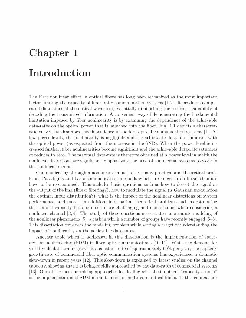
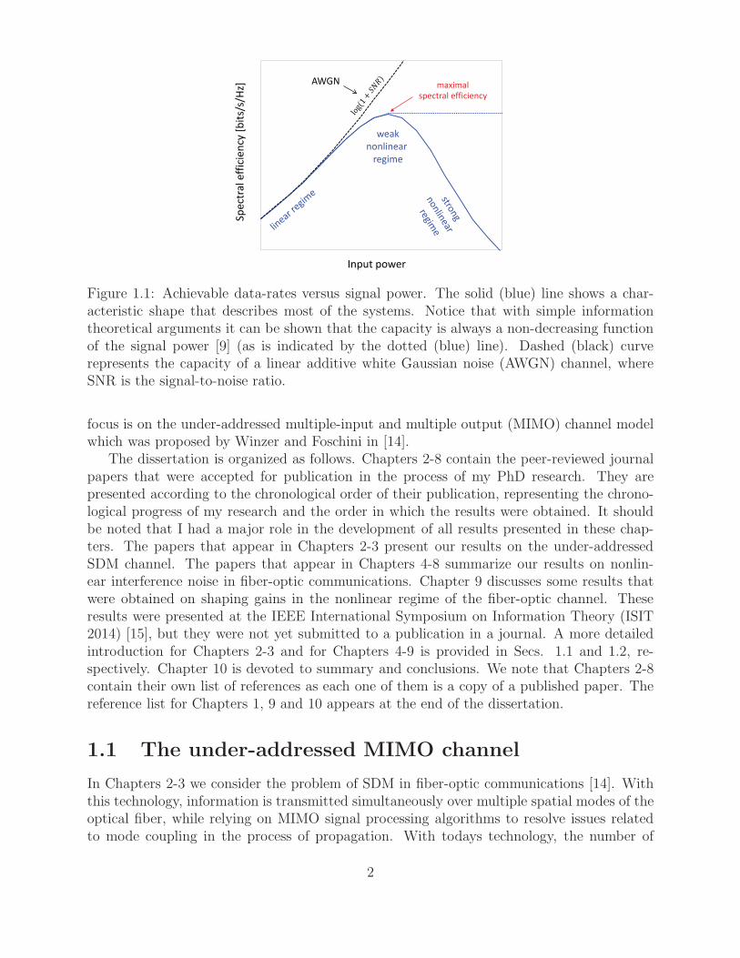
The Kerr nonlinear effect in optical fibers has long been recognized as the most importantfactor limiting the capacity of fiber-optic communication systems [1,2]. It produces compli-cated distortions of the optical waveform, essentially diminishing the receiver’s capability ofdecoding the transmitted information. A convenient way of demonstrating the fundamentallimitation imposed by fiber nonlinearity is by examining the dependence of the achievabledata-rates on the optical power that is launched into the fiber. Fig. 1.1 depicts a character-istic curve that describes this dependence in modern optical communication systems [1]. Atlow power levels, the nonlinearity is negligible and the achievable data-rate improves withthe optical power (as expected from the increase in the SNR). When the power level is in-creased further, fiber nonlinearities become significant and the achievable data-rate saturatesor reduces to zero. The maximal data-rate is therefore obtained at a power level in which thenonlinear distortions are significant, emphasizing the need of commercial systems to work inthe nonlinear regime.

Communicating through a nonlinear channel raises many practical and theoretical prob-lems. Paradigms and basic communication methods which are known from linear channelshave to be re-examined. This includes basic questions such as how to detect the signal atthe output of the link (linear filtering?), how to modulate the signal (is Gaussian modulationthe optimal input distribution?), what is the impact of the nonlinear distortions on systemperformance, and more. In addition, information theoretical problems such as estimatingthe channel capacity become much more challenging and cumbersome when considering anonlinear channel [3, 4]. The study of these questions necessitates an accurate modeling ofthe nonlinear phenomena [5], a task in which a number of groups have recently engaged [6–8].This dissertation considers the modeling problem while setting a target of understanding theimpact of nonlinearity on the achievable data-rates.

Another topic which is addressed in this dissertation is the implementation of space-division multiplexing (SDM) in fiber-optic communications [10, 11]. While the demand forworld-wide data traffic grows at a constant rate of approximately 60% per year, the capacitygrowth rate of commercial fiber-optic communication systems has experienced a dramaticslow-down in recent years [12]. This slow-down is explained by latest studies on the channelcapacity, showing that it is being rapidly approached by the data-rates of commercial systems[13]. One of the most promising approaches for dealing with the imminent “capacity crunch”is the implementation of SDM in multi-mode or multi-core optical fibers. In this context our

1

weak

nonlinear

regime

Input power

Sp

ect

ral

eff

icie

ncy

[b

its/

s/H

z]

maximal

spectral efficiency

The nonlinear distortions are proportional to the power of the signal …

AWGN

Figure 1.1: Achievable data-rates versus signal power. The solid (blue) line shows a char-acteristic shape that describes most of the systems. Notice that with simple informationtheoretical arguments it can be shown that the capacity is always a non-decreasing functionof the signal power [9] (as is indicated by the dotted (blue) line). Dashed (black) curverepresents the capacity of a linear additive white Gaussian noise (AWGN) channel, whereSNR is the signal-to-noise ratio.

focus is on the under-addressed multiple-input and multiple output (MIMO) channel modelwhich was proposed by Winzer and Foschini in [14].

The dissertation is organized as follows. Chapters 2-8 contain the peer-reviewed journalpapers that were accepted for publication in the process of my PhD research. They arepresented according to the chronological order of their publication, representing the chrono-logical progress of my research and the order in which the results were obtained. It shouldbe noted that I had a major role in the development of all results presented in these chap-ters. The papers that appear in Chapters 2-3 present our results on the under-addressedSDM channel. The papers that appear in Chapters 4-8 summarize our results on nonlin-ear interference noise in fiber-optic communications. Chapter 9 discusses some results thatwere obtained on shaping gains in the nonlinear regime of the fiber-optic channel. Theseresults were presented at the IEEE International Symposium on Information Theory (ISIT2014) [15], but they were not yet submitted to a publication in a journal. A more detailedintroduction for Chapters 2-3 and for Chapters 4-9 is provided in Secs. 1.1 and 1.2, re-spectively. Chapter 10 is devoted to summary and conclusions. We note that Chapters 2-8contain their own list of references as each one of them is a copy of a published paper. Thereference list for Chapters 1, 9 and 10 appears at the end of the dissertation.

1.1 The under-addressed MIMO channel

In Chapters 2-3 we consider the problem of SDM in fiber-optic communications [14]. Withthis technology, information is transmitted simultaneously over multiple spatial modes of theoptical fiber, while relying on MIMO signal processing algorithms to resolve issues relatedto mode coupling in the process of propagation. With todays technology, the number of

2

fiber modes that can be effectively supported for the transmission of information is limitedalmost exclusively by the complexity of the MIMO algorithms and by the speed of thesignal-processing hardware. As these technologies continuously improve with time, one mayconsider deploying multi-mode fibers admitting a larger number of spatial modes than can beprocessed today, with the intention of harvesting the full capacity of the fiber in the future.Such a solution, initially proposed and considered by Winzer and Foschini in [14], does notcome without a price. Part of the transmitted signal energy couples into fiber modes thatare not detected at the receiver, thereby resulting in the reduction of the achievable capacity.

The prime goal of the paper in Chapter 2 is to analyze the performance of the under-addressed channel with respect to the number of modes that are addressed by the transmitterand receiver. In the absence of sufficient experimental characterization, we adopt the as-sumptions of [14] and model the coupling between the modes as unitary. In this case thetransfer matrix is modeled as a block of size mr × mt within a uniformly drawn m × munitary matrix, where mt and mr represent the number of modes that are addressed bythe transmitter and receiver, respectively, and m represents the total number of availablemodes. By establishing the relation between the channel matrix and the Jacobi ensembleof random matrices [16–18], we find the distribution of the eigenvalues of the channel andderive explicit expressions to the channel capacity in the ergodic regime and to the outageprobability in the non-ergodic regime. An interesting outcome of the derivation is that zerooutage capacity can be obtained even when not all of the modes are detected by the receiver.

The paper which appears in Chapter 3 expands the results of Chapter 2 and furtheranalyzes the new channel model from a more information theoretical point of view. We reviewthe calculations of the ergodic capacity and outage probability in a more detailed manner andsupplement them with the calculation of the diversity-multiplexing tradeoff of the channel.We further provide a simple communication scheme that uses a channel-state feedback toobtain the zero-outage promise. In addition, we discuss the possibility of using the Jacobichannel as a model for fading MIMO channels where the size of the unitary matrix m definesthe “fading measure” of the channel, providing a way to model the statistical structure of thepower loss. For example, when m is equal to mr, the transfer matrix is simply composed oforthonormal columns: its elements (i.e., the path gains) are highly dependent and there is norandomness in the received power. As m becomes greater, the orthogonality of the columnsand rows of the transfer matrix fades, the dependency between the path gains becomesweaker and the power loss in the unaddressed receive outputs increases. Indeed, when m isvery large with respect to mt and mr, with proper normalization that compensates for theaverage power loss, the Jacobi fading model approaches to the Rayleigh model.

1.2 Nonlinear interference noise in fiber-optic commu-

nications

In a wavelength division multiplexed (WDM) environment, where several channels are mul-tiplexed into the fiber, nonlinear propagation phenomena can be classified as either intra-channel [19], or inter-channel [20] effects. Intra-channel distortions are those affecting anindividual WDM channel. Inter-channel distortions are those in which a given WDM chan-

3

nel is affected by the electric fields of the neighboring WDM channels that simultaneouslypropagate in the fiber. In principle, intra-channel distortions can be mitigated by meansof digital back propagation at the receiver [21], or pre-distortion at the transmitter [22].However, similar elimination of inter-channel distortions is considered impractical. The dif-ficulty is not only in the need of coherently detecting and jointly processing multiple WDMchannels, but also because of the unpredictable add-drop operations taking place in modernoptical networks, and the fact that the polarization states of different WDM channels evolverandomly and differently in the presence of polarization mode dispersion [23]. Inter-channelinterference is therefore customarily treated as noise [2], and hence we refer to it in whatfollows as nonlinear interference noise, or NLIN [24–30]. In this dissertation we focus oninter-channel nonlinear effects as they come into play in modern, dispersion uncompensatedfiber links with coherent optical detection. We additionally assume that the effect of non-linearity on the ASE noise, and its nonlinear interaction with the signal are negligible. Thisassumption is safely satisfied in most systems of practical relevance as well as in all systemconfigurations considered throughout the dissertation [2].

Two approaches to the analytical characterization of NLIN have so far been reported inthe literature. The first approach, which relies on analysis in the spectral domain, originatedfrom the group of P. Poggiolini at the Politecnico di Torino [6,31–33] and its derivation hasbeen recently generalized by Johannisson and Karlsson [34] and by Bononi and Serena [7].The model generated by this approach is commonly referred to as the Gaussian noise (GN)model and its implications have already been addressed in a number of studies [35–37]. Thesecond approach has been proposed by Mecozzi and Essiambre [38], and it is based on atime-domain analysis1. The results of the latter approach [38] are different from those ofthe former [6, 7, 34]. Most conspicuously, in the results of [6, 7, 34], the NLIN is treated asadditive Gaussian noise and its power-spectrum is totally independent of modulation format,whereas the theory of Mecozzi et al. predicts a strong dependence of the NLIN variance onthe modulation format, as well as the fact that in the presence of non-negligible intensitymodulation a large fraction of NLIN can be characterized as phase-noise.

In the paper presented in Chapter 4 we review the essential parts of the time-domaintheory of [38], as well as those of the frequency domain GN approach. We show that theassumption of statistical independence between non overlapping frequency components of thepropagating electric field is responsible for the fact that the NLIN in Refs. [6, 7, 34] appearsto be independent of modulation format. We supplement the NLIN variance obtained in thefrequency domain analysis [31] with an extra term that follows from fourth-order frequencycorrelations. This work has been followed upon by the authors of [6], and a new enhancedGN model that relies on the findings of our analysis has been published subsequently in [41].We believe that the results of Chapter 4 and the followup work of [41] settle the discrepancybetween the frequency domain approach [6, 7, 34] and the time-domain theory of [38]2.

In the paper presented in Chapter 5, we revisit the problem of estimating the nonlinearchannel capacity. A common feature of capacity estimates published so far [1, 2] is thatthey treat the intra-channel nonlinear interference as a cancelable noise while treating the

1Additional time-domain models for inter-channel NLIN were developed in Refs. [8, 39] and for intra-channel NLIN in Ref. [40].

2An additional frequency-domain analysis has been recently published [42], showing similar dependenceof NLIN spectrum on the high order moments of the transmitted signal.

4

inter-channel nonlinear interference as additive, white noise which is independent of the datatransmitted on the channel of interest. In reality, in the presence of chromatic dispersion,different WDM channels propagate at different velocities so that every symbol in the chan-nel of interest interacts with multiple symbols of every interfering channel. Consequently,adjacent symbols in the channel of interest are disturbed by essentially the same collectionof interfering pulses and therefore they are affected by nonlinearity in a highly correlatedmanner. In addition, as demonstrated in Chapter 4, one of the most pronounced manifes-tations of nonlinearity is in the form of phase-noise. We show that by taking advantage ofthe fact that a large fraction of the nonlinear interference is in the form of phase-noise, andby accounting for the long temporal correlations of this noise, the capacity of the fiber-opticchannel is notably higher than what is currently assumed. This advantage is translated intothe doubling of the link distance for a fixed transmission rate. The impact of these resultson practical systems is further examined in Chapter 7.

We follow-up the work of Chapter 4 and further explore the statistical properties of NLINin Chapter 6. We examine the significance of nonlinear phase-noise and the importance ofthe modulation format dependence of NLIN variance with respect to system parameterssuch as the link-length, span-length, amplification scheme, and more. We show that thesignificance of phase-noise and the modulation format dependence are largest in the case ofa single amplified span, or in a system of arbitrary length that uses distributed amplification;their distinctness reduces somewhat in multi-span systems with lumped amplification andwith a span-length much larger than the fibers effective length. In order to facilitate futureresearch of this problem, we provide a Matlab program that implements a computationallyefficient algorithm for computing the overall NLIN variance. This Matlab program wasfurther developed into an online web application that is available at http://nlinwizard.eng.tau.ac.il/.

In the first part of the invited paper presented in Chapter 7 we extend the work reportedin Chapters 4 and 6 and generalize the time-domain model to the case of polarization-multiplexed transmission. We characterize the nature of NLIN in this case and explore thedependence of the relevant NLIN features on the parameters of the system. In the second partof the paper we show that the effect of NLIN is equivalent to a linear time-varying inter-symbol-interference (ISI) (where the zeroth-order ISI coefficient manifests itself as phase-noise, as was discussed in Chapter 4-6). We propose a nonlinear interference mitigationscheme that exploit the temporal correlations of the ISI terms to track, estimate and canceltheir effect by using linear fast-adaptive equalization. We evaluate the potential benefit ofsuch schemes and discuss the implications on system design.

In the paper of Chapter 8 we model the build-up of NLIN by considering the pulse-collision dynamics in the time domain. We show that the fundamental interactions can beclassified as two-pulse, three-pulse, or four-pulse collisions and they can be either complete, orincomplete. Each type of collision is shown to have its unique signature and the overall natureof NLIN is determined by the relative importance of the various classes of pulse collisions ina given WDM system. The most important contributions to NLIN follow from two-pulse andfour-pulse collisions. While the contribution of two-pulse collisions is in the form of phase-noise and polarization-state-rotation with strong dependence on modulation format, four-pulse collisions generate complex circular noise whose variance is independent of modulationformat. In addition, two-pulse collisions are strongest when the collision is complete, whereas

5

four-pulse collisions are strongest when the collision is incomplete. We show that two-pulsecollisions dominate the formation of NLIN in short links with lumped amplification, or inlinks with distributed amplification extending over arbitrary length. In long links usinglumped amplification the relative significance of four-pulse collisions increases, emphasizingthe circularity of the NLIN while reducing its dependence on modulation format.

Finally, in Chapter 9 we examine methods for suppressing NLIN by shaping the inputconstellation. We show that by using a ball shaped input the nonlinear penalty can besignificantly reduced. The potential shaping gain in the nonlinear fiber-optic channel istherefore not only in reducing the average transmission power, as in linear AWGN channels[43,44], but also in suppressing the affect of nonlinearity. We show that the maximum shapinggain in certain fiber-optic scenarios can be more than 1.53dB, which is the ultimate shapinggain in linear AWGN channels. Furthermore, while the “linear” shaping gain monotonicallyincreases with the number of dimensions of the shaping region, the maximum shaping gainfrom suppressing the NLIN is obtained with a finite-dimensional ball shaped input. Theresults of this chapter also relate to the problem of finding the optimum input distributionwhich maximizes the channel mutual information, showing that Gaussian distribution maybe sub-optimal in the nonlinear optical channel.

We note that our analysis throughout this dissertation focuses on inter-channel nonlin-earities resulted from XPM only while ignoring FWM contributions. As is evident fromsimulations [24, 41], the contribution of FWM to NLIN is of negligible importance in allscenarios examined throughout this dissertation as well as in most of current commercialsystems. We note however that FWM contributions may become important in certain sys-tems employing multi-subcarrier transmission [45] or operating over very low dispersionfibers [24]. The significance of FWM in these cases can be further investigated by using thetheoretical predictions of the NLIN Wizard.

6

Chapter 2

The Under Addressed Optical MIMO

Channel: Capacity and OutageRonen Dar, Meir Feder andMark Shtaif, “The under-addressed optical multiple-input, multiple-output channel: capacity and outage,” Optics letters, vol. 37, pp. 3150–3152 (August 2012)

2.1 Abstract

We study an optical space-division multiplexed system where the number of modes that areaddressed by the transmitter and receiver is allowed to be smaller than the total numberof optical modes supported by the fiber. This situation will be of relevance if, for instance,fibers supporting more modes than can be processed with current MIMO technology aredeployed with the purpose of future-proof installation. We calculate the ergodic capacityand the outage probability of the link and study their dependence on the number of addressedmodes at the transmitter and receiver.

2.2 Introduction and results

One of the most intensely explored approaches for dealing with the imminent capacity crunchof optical communications systems [1] is the implementation of space division multiplexing(SDM) in multi-mode optical fibers [2–6]. With this approach, information is transmittedsimultaneously over multiple spatial modes of the optical fiber, while relying on multiple-input and multiple-output (MIMO) signal processing algorithms to resolve issues related tomode coupling in the process of propagation. With today’s technology, the number of fibermodes that can be effectively supported for the transmission of information is limited almostexclusively by the complexity of the MIMO algorithms and by the speed of signal-processinghardware. As these technologies continuously improve with time, one may consider deployingmulti-mode fibers admitting a larger number of spatial modes than can be processed today,with the intention of harvesting the full capacity of the fiber in the future. Such a solution,initially proposed and considered by Winzer and Foschini in [3], does not come without aprice. Part of the transmitted signal energy couples into fiber modes that are not detected

7

at the receiver, thereby resulting in the reduction of achievable capacity. In what follows, werefer to the multi-mode fiber-optic channel in which not all supported modes are coupled totransmitters or receivers, as the under-addressed MIMO channel. Analysis of its performanceis the prime goal of this work.

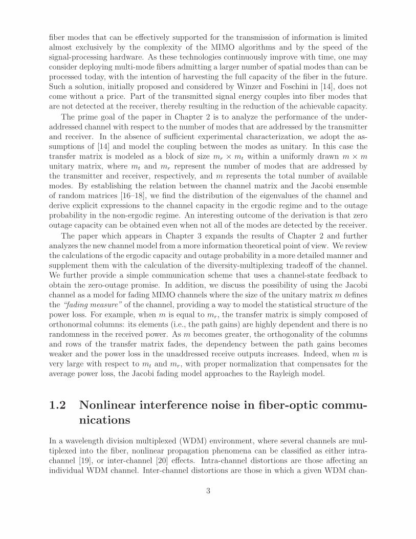
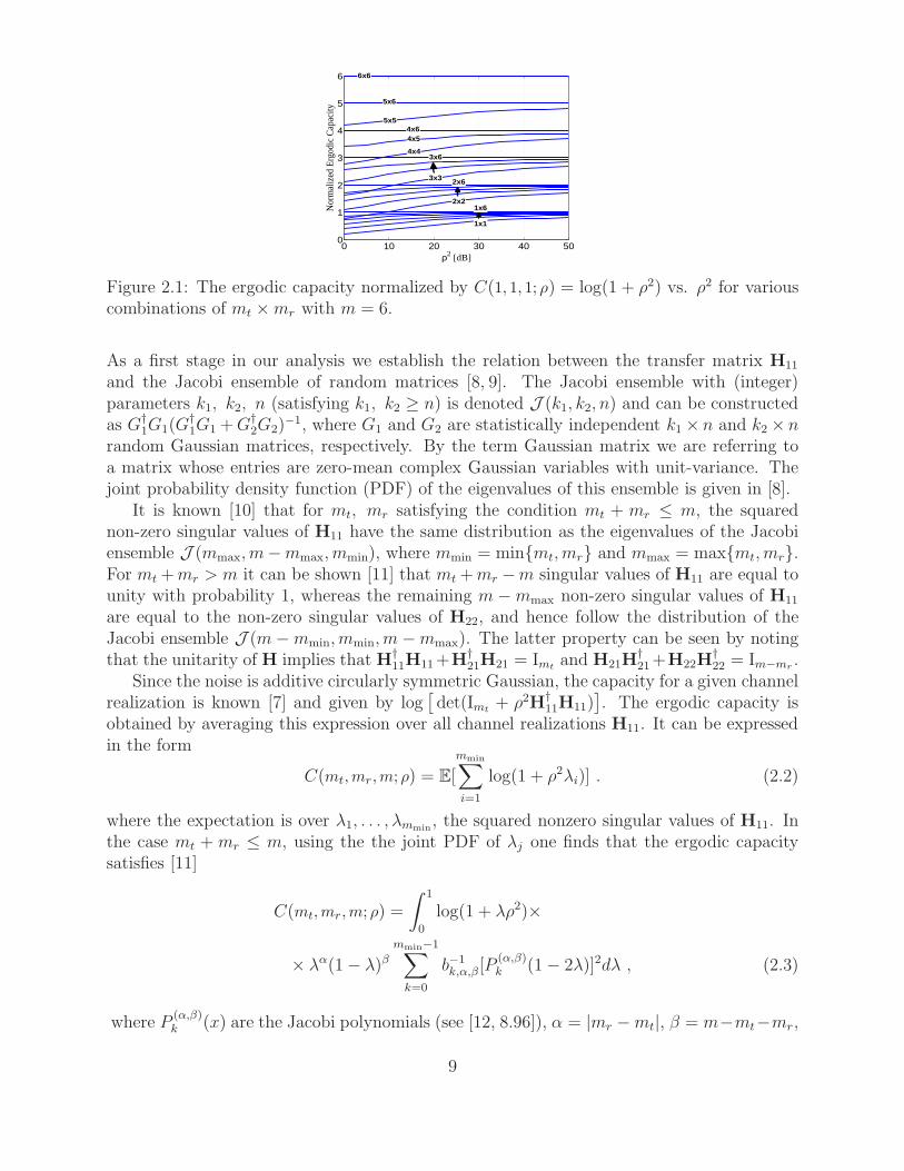
We consider a system using a total of m scalar modes (counting both spatial modes andpolarizations) and where the number of modes addressed by the transmitter and receiver aremt and mr, respectively. We explore two distinct regimes of operation, referred to as theergodic and the non-ergodic regimes [7]. In the ergodic regime, a single frame of the error-correcting code samples the entire channel statistics, whereas in the non-ergodic regime,the channel within each code-frame is assumed to be constant. The ergodic regime can berelevant if schemes actively randomizing fiber mode-coupling on a time-scale much shorterthan the the error-correcting code-frame are introduced. Alternatively, in the fiber-opticalscenario, if coding is implemented in the spectral domain, the ergodic assumption applieswhen the channel decorrelates quickly in frequency. A situation that characterizes systemswith high modal dispersion [5]. In the ergodic regime, performance is evaluated in termsof the ergodic capacity, which is the channel capacity averaged with respect to all channelrealizations. In the non-ergodic regime, performance is characterized in terms of the systemoutage probability. We derive these quantities analytically and present their dependence onm, mt and mr. A particularly interesting outcome of our study is that when mt +mr > m,a throughput equivalent to mt+mr −m decoupled single-mode channels can be guaranteed.In the fast-changing channel regime this implies that the ergodic capacity is never smallerthan (mt +mr −m) single-input single-output (SISO) channels, whereas in the non-ergodicregime a throughput equivalent to (mt +mr −m) SISO channels can be achieved with zerooutage probability.

In the absence of sufficient experimental characterization, we adopt the description ofthe multi-mode fiber as a unitary system with strong mode-coupling, as was used in mostprevious studies [3–6] of the multi-mode transmission problem. By doing so, we ignore theeffects of mode-dependent losses and justify the description of the overall m × m transfermatrix H as a random instantiation drawn uniformly from the ensemble of all m×m unitarymatrices (Haar distributed). In addition, as was done in [3], we assume that the averagepower generated by each of the mt transmitters is constant, regardless of the value of mt.Under these conditions the channel can be described as

y = ρH11x+ z , (2.1)

where the vector x containing mt complex components, represents the transmitted signal,the vector y containing mr complex components, represents the received signal, and z ac-counts for the presence of additive Gaussian noise. The mr components of z are statisticallyindependent, circularly symmetric complex zero-mean Gaussian variables of unit energyE(|zj |2) = 1, and the components of x are constrained such that the average energy of eachcomponent is equal to 1, i.e., E(|xj |2) = 1 for all j. The term ρ is proportional to the opticalpower per excited mode so that ρ2 is equal to the signal-to-noise ratio (SNR) in the singlemode (m = 1) case. The matrix H11 is a block of size mr ×mt within the m ×m randomunitary matrix H

H =

[H11 H12

H21 H22

].

8

0 10 20 30 40 500

1

2

3

4

5

6

ρ2 [dB]

Nor

mal

ized

Erg

odic

Cap

acity

6x6

4x43x6

2x6

1x1

2x21x6

3x3

4x5

5x5

5x6

4x6

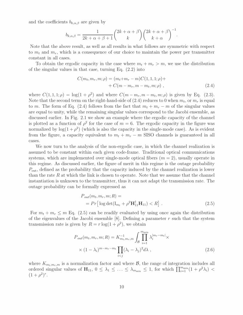
Figure 2.1: The ergodic capacity normalized by C(1, 1, 1; ρ) = log(1 + ρ2) vs. ρ2 for variouscombinations of mt ×mr with m = 6.

As a first stage in our analysis we establish the relation between the transfer matrix H11

and the Jacobi ensemble of random matrices [8, 9]. The Jacobi ensemble with (integer)parameters k1, k2, n (satisfying k1, k2 ≥ n) is denoted J (k1, k2, n) and can be constructedas G†

1G1(G†1G1 +G†

2G2)−1, where G1 and G2 are statistically independent k1 × n and k2 × n

random Gaussian matrices, respectively. By the term Gaussian matrix we are referring toa matrix whose entries are zero-mean complex Gaussian variables with unit-variance. Thejoint probability density function (PDF) of the eigenvalues of this ensemble is given in [8].

It is known [10] that for mt, mr satisfying the condition mt + mr ≤ m, the squarednon-zero singular values of H11 have the same distribution as the eigenvalues of the Jacobiensemble J (mmax, m−mmax, mmin), where mmin = minmt, mr and mmax = maxmt, mr.For mt +mr > m it can be shown [11] that mt +mr −m singular values of H11 are equal tounity with probability 1, whereas the remaining m −mmax non-zero singular values of H11

are equal to the non-zero singular values of H22, and hence follow the distribution of theJacobi ensemble J (m−mmin, mmin, m−mmax). The latter property can be seen by notingthat the unitarity of H implies that H†

11H11+H†21H21 = Imt

and H21H†21+H22H

†22 = Im−mr

.Since the noise is additive circularly symmetric Gaussian, the capacity for a given channel

realization is known [7] and given by log[det(Imt

+ ρ2H†11H11)

]. The ergodic capacity is

obtained by averaging this expression over all channel realizations H11. It can be expressedin the form

C(mt,mr,m; ρ) = E[

mmin∑

i=1

log(1 + ρ2λi)] . (2.2)

where the expectation is over λ1, . . . , λmmin, the squared nonzero singular values of H11. In

the case mt + mr ≤ m, using the the joint PDF of λj one finds that the ergodic capacitysatisfies [11]

C(mt,mr,m; ρ) =

∫ 1

0

log(1 + λρ2)×

× λα(1− λ)βmmin−1∑

k=0

b−1k,α,β[P

(α,β)k (1− 2λ)]2dλ , (2.3)

where P(α,β)k (x) are the Jacobi polynomials (see [12, 8.96]), α = |mr −mt|, β = m−mt−mr,

9

and the coefficients bk,α,β are given by

bk,α,β =1

2k + α + β + 1

(2k + α+ β

k

)(2k + α + β

k + α

)−1

.

Note that the above result, as well as all results in what follows are symmetric with respectto mt and mr, which is a consequence of our choice to maintain the power per transmitterconstant in all cases.

To obtain the ergodic capacity in the case where mt +mr > m, we use the distributionof the singular values in that case, turning Eq. (2.2) into

C(mt,mr,m; ρ) = (mt+mr −m)C(1, 1, 1; ρ)+

+ C(m−mr,m−mt,m; ρ) , (2.4)

where C(1, 1, 1; ρ) = log(1 + ρ2) and where C(m−mr,m−mt,m; ρ) is given by Eq. (2.3).Note that the second term on the right-hand-side of (2.4) reduces to 0 whenmt, ormr is equalto m. The form of Eq. (2.4) follows from the fact that mt +mr −m of the singular valuesare equal to unity, while the remaining singular values correspond to the Jacobi ensemble, asdiscussed earlier. In Fig. 2.1 we show an example where the ergodic capacity of the channelis plotted as a function of ρ2 for the case of m = 6. The ergodic capacity in the figure wasnormalized by log(1 + ρ2) (which is also the capacity in the single-mode case). As is evidentfrom the figure, a capacity equivalent to mt + mr − m SISO channels is guaranteed in allcases.

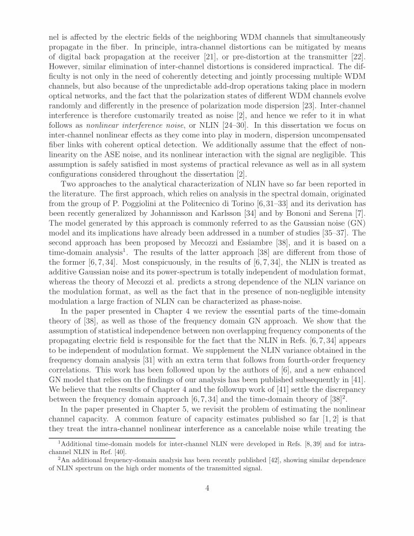
We now turn to the analysis of the non-ergodic case, in which the channel realization isassumed to be constant within each given code-frame. Traditional optical communicationssystems, which are implemented over single-mode optical fibers (m = 2), usually operate inthis regime. As discussed earlier, the figure of merit in this regime is the outage probabilityPout, defined as the probability that the capacity induced by the channel realization is lowerthan the rate R at which the link is chosen to operate. Note that we assume that the channelinstantiation is unknown to the transmitter, thus it can not adapt the transmission rate. Theoutage probability can be formally expressed as

P out(mt,mr,m;R) =

= Pr[log det(Imt

+ ρ2H†11H11) < R

]. (2.5)

For mt +mr ≤ m Eq. (2.5) can be readily evaluated by using once again the distributionof the eigenvalues of the Jacobi ensemble [8]. Defining a parameter r such that the systemtransmission rate is given by R = r log(1 + ρ2), we obtain

P out(mt,mr,m;R) = K−1mt,mr ,m

∫

B

mmin∏

i=1

λ|mr−mt|i ×

× (1− λi)m−mr−mt

∏

i<j

(λi − λj)2dλ , (2.6)

where Kmt,mr ,m is a normalization factor and where B, the range of integration includes allordered singular values of H11, 0 ≤ λ1 ≤ . . . ≤ λmmin

≤ 1, for which∏mmin

i=1 (1 + ρ2λi) <(1 + ρ2)r.

10

0 1 2 3 4 5 610

−5

10−4

10−3

10−2

10−1

100

r=R/log(1+ρ2)

Out

age

Pro

babi

lity

4x43x6

3x32x6

2x21x11x6 4x54x6 6x6

5x55x6

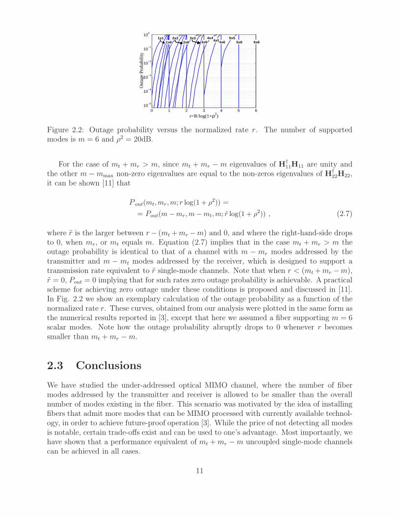
Figure 2.2: Outage probability versus the normalized rate r. The number of supportedmodes is m = 6 and ρ2 = 20dB.

For the case of mt +mr > m, since mt +mr −m eigenvalues of H†11H11 are unity and

the other m−mmax non-zero eigenvalues are equal to the non-zeros eigenvalues of H†22H22,

it can be shown [11] that

P out(mt,mr,m; r log(1 + ρ2)) =

= Pout(m−mr,m−mt,m; r log(1 + ρ2)) , (2.7)

where r is the larger between r− (mt+mr −m) and 0, and where the right-hand-side dropsto 0, when mr, or mt equals m. Equation (2.7) implies that in the case mt +mr > m theoutage probability is identical to that of a channel with m − mr modes addressed by thetransmitter and m − mt modes addressed by the receiver, which is designed to support atransmission rate equivalent to r single-mode channels. Note that when r < (mt +mr −m),r = 0, Pout = 0 implying that for such rates zero outage probability is achievable. A practicalscheme for achieving zero outage under these conditions is proposed and discussed in [11].In Fig. 2.2 we show an exemplary calculation of the outage probability as a function of thenormalized rate r. These curves, obtained from our analysis were plotted in the same form asthe numerical results reported in [3], except that here we assumed a fiber supporting m = 6scalar modes. Note how the outage probability abruptly drops to 0 whenever r becomessmaller than mt +mr −m.

2.3 Conclusions

We have studied the under-addressed optical MIMO channel, where the number of fibermodes addressed by the transmitter and receiver is allowed to be smaller than the overallnumber of modes existing in the fiber. This scenario was motivated by the idea of installingfibers that admit more modes that can be MIMO processed with currently available technol-ogy, in order to achieve future-proof operation [3]. While the price of not detecting all modesis notable, certain trade-offs exist and can be used to one’s advantage. Most importantly, wehave shown that a performance equivalent of mt +mr −m uncoupled single-mode channelscan be achieved in all cases.

11

Acknowledgement

The authors wish to thank Amir Dembo for his useful comments. Mark Shtaif acknowledgesfinancial support by TeraSanta consortium and by Alcatel-Lucent within the framework ofGreen Touch. The research was partially supported by the Israel Science Foundation, grantNo. 634/09.

12

Bibliography

[1] A. R. Chraplyvy, “The coming capacity crunch,”European Conference on Optical Com-munication 2009 (ECOC09), plenary talk (2009).

[2] S. Randel, R. Ryf, A. Sierra, P.J. Winzer, A.H. Gnauck, C.A. Bolle, R-J. Essiambre,D.W. Peckham, A. McCurdy, and R. Lingle, “6 × 56-Gb/s mode-division multiplexedtransmission over 33-km few-mode fiber enabled by 6×6 MIMO equalization,”Opt. Ex-press19, 16697–16707 (2011).

[3] P. J. Winzer and G. J. Foschini, “MIMO capacities and outage probabilities in spatiallymultiplexed optical transport systems,” Opt. Express19, 16680-16696 (2011).

[4] K.-P. Ho and J. M. Kahn, “Frequency Diversity in Mode-Division Multiplexing Sys-tems,” J. Lightwave Technol. 29, 3719–3726 (2011).

[5] C. Antonelli, A. Mecozzi, M. Shtaif, and P. J. Winzer, “Stokes-space analysis of modaldispersion in fibers with multiple mode transmission,”Opt. Express20, 11718–11733(2012).

[6] K.-P. Ho and J. M Kahn, “Statistics of group delays in multi-mode fibers with strongmode coupling,”J. Lightwave Technol. 29, 3119–3128 (2011).

[7] I. E. Telatar, “Capacity of multi-antenna Gaussian channels,” European Transactionson Telecommunications 10, 585-595 (1999).

[8] R. J. Muirhead, Aspects of Multivariate Statistical Theory (Wiley, 1982).

[9] A. Edelman and N. Raj Rao, “Random matrix theory,” Acta Numerica 14, 233-297(2005).

[10] A. Edelman and B. D. Sutton, “The beta-Jacobi matrix model, the CS decomposition,and generalized singular value problems,” Foundations of Computational Mathematics8, 259-285 (2008).

[11] R. Dar, M. Feder and M. Shtaif, “The Jacobi MIMO Channel,” available onhttp://arxiv.org/abs/1202.0305.

[12] I. S. Gradshteyn and I. M. Ryzhik, Table of Integrals, Series, and Products (AcademicPress, 1980).

13

Chapter 3

The Jacobi MIMO ChannelRonen Dar, Meir Feder and Mark Shtaif, “The Jacobi MIMO channel,” IEEE Transactionson Information Theory, vol. 59, pp. 2426–2441 (April 2013)

3.1 abstract

This paper presents a new fading model for MIMO channels, the Jacobi fading model. Itasserts that H, the transfer matrix which couples the mt inputs into mr outputs, is a sub-matrix of anm×m random (Haar-distributed) unitary matrix. The (squared) singular valuesof H follow the law of the classical Jacobi ensemble of random matrices; hence the nameof the channel. One motivation to define such a channel comes from multimode/multicoreoptical fiber communication. It turns out that this model can be qualitatively different thanthe Rayleigh model, leading to interesting practical and theoretical results. This paper firstevaluates the ergodic capacity of the channel. Then, it considers the non-ergodic case, whereit analyzes the outage probability and the diversity-multiplexing tradeoff. In the case wherek = mt +mr −m > 0 it is shown that at least k degrees of freedom are guaranteed not tofade for any channel realization, enabling a zero outage probability or infinite diversity orderat the corresponding rates. A simple scheme utilizing (a possibly outdated) channel statefeedback is provided, attaining the no-outage guarantee. Finally, noting that as m increases,the Jacobi model approaches the Rayleigh model, the paper discusses the applicability ofthe model in other communication scenarios.

3.2 Introduction

In Multi-Input Multi-Output (MIMO) channels a vector x of mt signals is transmitted, avector y of mr signals is received, and an mr ×mt random matrix H represents the couplingof the input into the output so that the received vector is y = Hx + z where z is a noisevector. In this paper we consider a channel matrix H which is a sub-matrix of a Haar-distributed unitary matrix, i.e., drawn uniformly from the ensemble of all m × m unitarymatrices, m ≥ mt, mr.

The three classical and most well-studied random matrix ensembles are the Gaussian,Wishart and Jacobi (also known as MANOVA) ensembles [1–4]. A common model for the

15

channel matrix H in fading wireless communication is a matrix with independent Gaussianelements (also known as the Rayleigh model). In that case, H†H is a Wishart matrix . Forthe model assumed in this paper, H†H follows the Jacobi ensemble. It turns out that thismodel is both practically useful and qualitatively different than other fading models such asthe Rayleigh [5–7], Rician [8–10] and Nakagami [10–13].

Jacobi ensembles, forming an important part of classical random matrix ensembles, areof considerable interest in connection with multivariate statistics and random matrix the-ory [1–3]. These ensembles have been successfully applied in several problems. One notableexample is related to quantum conductance/transmission in mesoscopic systems [4, 14–18],where scattering is modeled by a random unitary matrix (owing to flux conservation) andthe blocks of unitary matrix are then the transmission/reflection matrices which govern theconductance/transmission properties. This paper provides another application in communi-cation theory.

The motivation to introduce the Jacobi channel comes from recent developments in opti-cal fiber communication. The expected capacity crunch in long haul optical fibers [19,20] ledto proposals for “space-division multiplexing” (SDM) [21, 22], that is to have several linksat the same fiber, by either multiple single-mode fiber strands within a fiber cable, multi-ple cores within a multi-core fiber, or multiple modes within a multi-mode waveguide. AnSDM system with m parallel transmission paths per wavelength can potentially multiply thethroughput of a certain link by a factor of m. Since m can potentially be chosen very large,SDM technology is highly scalable. Now, a significant crosstalk between the optical pathsraises the need for MIMO signal processing techniques. Unfortunately, for large size MIMO(large m) this is unfeasible currently in the optical rates. Assuming that faster computationwill be available in the future and having in mind that replacing optical fibers to supportSDM is a long and expensive procedure, a long term design is sought after. To that end andmore, it was proposed to design an optical system that can support relatively large numberof paths for future use, but at start to address only some of the paths. In this scenario thechannel can be modeled as a sub-matrix of a larger unitary matrix, i.e., the Jacobi model isapplicable.

This under-addressed channel is discussed in [23] where simulations of the capacities andoutage probabilities were presented. In this paper we further analyze the channel in theergodic and non-ergodic settings, where we provide analytical expression for the capacity,outage probability and the diversity-multiplexing tradeoff. It should be noted that in opticalsystems the outage probability is an important measure, required to be very low. Evidently,since the entire channel matrix is unitary, when all paths are addressed a zero outage prob-ability can be attained for any transmission rate. An interesting result that comes out ofthis work is that there are situations, where a partial number of paths are addressed, yet anumber of streams are guaranteed to experience zero outage. Thus, choosing the numberof addressed paths and the corresponding rate is a very critical design element that highlyreflects on the system outage and performance. A preliminary description of our work, inthe context of the SDM optical channel is provided in [24].

A possibly practical outcome of this work is a simple communication scheme, with channelstate feedback, that achieves the highest rate possible with no outage. The scheme workseven when the feedback is “outdated”, and it allows simple decoding with no complicatedMIMO signal processing, making it plausible for optical communication. We note that while

16

our theoretical findings indicate that the no-outage promise can be attained with no feedback,the quest for such simple schemes is open.

As noted above, the motivation for this work comes from optical fiber communication.Yet, the application of the Jacobi model and the insights that follow from it may be relevantin other cases, such as in-line communication and even wireless communication. While aconstant can be applied to account for the average power loss in the medium, the randomnessstructure of the loss can be modeled using the Jacobi model. As m increases with respectto mt, mr, the randomness of the absolute received power increases. Evidently, in typicalwireless communication, a large fraction of the energy is not captured, and so the channelcan be modeled as a small sub-matrix of a large unitary matrix. Indeed, it will be shownthat as m becomes larger in comparison to mt, mr, the Jacobi model (up to a normalizingconstant) approaches the Rayleigh model.

The paper is organized as follows. We start by defining the system model and presentingthe channel statistics in Section 3.3. An interesting transition threshold is revealed: whenthe number of addressed paths is large enough, so that k = mt +mr −m > 0, the statisticsof the problem changes. Using this observation we give analytic expressions for the ergodiccapacity in Section 3.4. In Section 3.5 we analyze the outage probabilities in the non-ergodicchannel and show that for k > 0 a strictly zero outage probability is obtainable for k degreesof freedom. Following this finding, we present in Section 3.6 a new communication schemewhich exploits a channel state feedback to achieve zero outage probability. Section 3.7 discussthe diversity-multiplexing tradeoff of the channel where we show an absorbing difference inthe maximum diversity gain between the Rayleigh fading and Jacobi channels. Section 3.9discusses the results.

3.3 System Model and Channel Statistics

We consider a space-division multiplexing (SDM) system that supportsm spatial propagationpaths. In tribute to optical communication, in particular multi-mode optical fibers, the initialmotivation for this work, we shall refer to these links as modes. Assuming a unitary couplingamong all transmission modes the overall transfer matrix H can be described as an m×munitary matrix, where each entry hij represents the complex path gain from transmittedmode i to received mode j. We further assume a uniformly distributed unitary coupling,that is, H is drawn uniformly from the ensemble of all m × m unitary matrices (Haardistributed). Considering a communication system where mt ≤ m and mr ≤ m modes arebeing addressed by the transmitter and receiver, respectively, the effective transfer matrix isa truncated version of H. Under these conditions the channel can be described as

y =√ρ H11x+ z , (3.1)

where the vector x containing mt complex components, represents the transmitted signal,the vector y containing mr complex components, represents the received signal, and z ac-counts for the presence of additive Gaussian noise. The mr components of z are statisticallyindependent, circularly symmetric complex zero-mean Gaussian variables of unit energyE(|zj |2) = 1. The components of x are constrained such that the average energy of each

17

component is equal to 1, i.e., E(|xj |2) = 1 for all j 1. The term ρ ≥ 0 is proportional tothe power per excited mode so that it equals to the signal-to-noise ratio in the single modecase (m = 1). The matrix H11 is a block of size mr ×mt within the m×m random unitarymatrix H

H =

[H11 H12

H21 H22

]. (3.2)

As a first stage in our analysis we establish the relation between the transfer matrixH11 and the Jacobi ensemble of random matrices [1–3]. Limiting our discussion to complexmatrices we state the following definitions:

Definition 1 (Gaussian matrices). G(m,n) is m × n matrix of i.i.d complex entries dis-tributed as CN (0, 1).

Definition 2 (Wishart ensemble). W(m,n), where m ≥ n, is n×n Hermitian matrix whichcan be constructed as A†A, where A is G(m,n).Definition 3 (Jacobi ensemble). J (m1, m2, n), where m1, m2 ≥ n, is n × n Hermitianmatrix which can be constructed as A(A+B)−1, where A and B are W(m1, n) and W(m2, n),respectively.

The first two definitions relate to wireless communication [7]. We claim here that thethird classical ensemble, the Jacobi ensemble, is relevant to this channel model by relatingits eigenvalues to the singular values of H11. To that end we quote the well-known [1,4] jointprobability density function (PDF) of the ordered eigenvalues 0 ≤ λ1 ≤ . . . ≤ λn ≤ 1 of theJacobi ensemble J (m1, m2, n)

f(λ1, . . . , λn) = K−1m1,m2,n

n∏

i=1

λm1−ni (1− λi)

m2−n∏

i<j

(λi − λj)2 , (3.3)

where Km1,m2,n is a normalizing constant. We say that n variables follow the law of theJacobi ensemble J (m1, m2, n) if their joint distribution follows (3.3).

We shall now present the explicit distribution of the channel’s singular values by distin-guishing between the following two cases:

3.3.1 Case I - mt +mr ≤ m

In [25, Theorem 1.5] it was shown that for mt, mr satisfying the conditions mt ≤ mr andmt + mr ≤ m, the eigenvalues of H†

11H11 have the same distribution as the eigenvalues ofthe Jacobi ensemble J (mr, m−mr, mt). For mt, mr satisfying mt > mr and mt +mr ≤ m,since H† share the same distribution with H, the eigenvalues of H11H

†11 follow the law of

the Jacobi ensemble J (mt, m−mt, mr). Combining these two results, we can say that thesquared non-zero singular values of H11 have the same distribution as the eigenvalues of theJacobi ensemble J (mmax, m−mmax, mmin), where here and throughout this paper we denotemmax = maxmt, mr and mmin = minmt, mr.

1The constant per-mode power constraint, as opposed to the constant total power constraint often usedin wireless communication, is motivated by the optical fiber nonlinearity limitation. Nevertheless, the totalpower constraint will be considered as well when needed.

18

3.3.2 Case II - mt +mr > m

When the sum of transmit and receive modes, mt + mr, is larger than the total availablemodes, m, the statistics of the singular values change. Clearly, when H11 is the completeunitary matrix (mt = mr = m), all singular values are one. Thus, having in mind that thecolumns of H are orthonormal, one can think of mt +mr > m as a transition threshold inwhich the size of H11 is large enough with respect to the size of the complete unitary matrixto change the singularity statistics. The following Lemma provides the joint distribution ofthe singular values of H11, showing that for any realization of H11 there are mt +mr −msingular values which are 1. This Lemma is a Corollary of a result of Paige and Saunders [26],however its proof is given here for completeness.

Lemma 1. Let H be an m×m unitary matrix, divided into blocks as in (3.2), where H11 is anmr×mt block with mt+mr > m. Thenmt+mr−m eigenvalues of H†

11H11 are 1, mt−mmin are0, and m−mmax equal to the non-zero eigenvalues of H22H

†22; if H is Haar distributed these

m−mmax eigenvalues follow the law of the Jacobi ensemble J (m−mmin, mmin, m−mmax).

Proof. Since H is unitary we can write

H†11H11 +H†

21H21 = Imt(3.4)

andH21H

†21 +H22H

†22 = Im−mr

. (3.5)

Let λ(11)i mt

i=1 and λ(21)i mt

i=1 be the eigenvalues of H†11H11 and H†

21H21, respectively. From(3.4) we can write

λ(11)i = 1− λ

(21)i ∀ i = 1, . . . , mt . (3.6)

Since H21 is a block of size (m − mr) × mt where m − mr < mt, H†21H21 has (at least)

mt +mr −m zero eigenvalues. Following (3.6), H†11H11 has mt +mr −m eigenvalues which

are 1. Now, let λ(21)i m−mr

i=1 and λ(22)i m−mr

i=1 be the eigenvalues of H21H†21 and H22H

†22,

respectively. From (3.5) we can write

λ(21)i = 1− λ

(22)i ∀ i = 1, . . . , m−mr . (3.7)

Since for any matrix A, A†A and AA† share the same non-zero eigenvalues we can combine(3.6) and (3.7) to conclude that the additional m − mr eigenvalues of H†

11H11 are equal tothe m − mr eigenvalues of H22H

†22. Note that mt − mmin of them are 0. Since the above

arguments hold for any unitary matrix, and since H22 is a block of size (m−mr)× (m−mt),when H is Haar distributed the results of subsection 3.3.1 can be applied, which completesthe proof.

Lemma 1 reveals an interesting algebraic phenomenon: k = maxmt+mr−m, 0 singularvalues ofH11 are 1 for any realization ofH. This provides some powerful results in the contextof Jacobi fading channels. For example, the channel’s power ‖H11‖2F , where ‖A‖F denotesthe Frobenius norm of A, is guaranteed to be at least k. Furthermore, H11 always comprisesan unfaded k-dimensional subspace. In what follows we show that this implies a lower boundon the ergodic capacity, an achievable zero outage probability and an “unbounded” diversitygain for certain rates.

19

3.4 The Ergodic Case

In the ergodic scenario the channel is assumed to be rapidly changing so that the transmittedsignal samples the entire channel statistics. We further assume that the channel realizationat each symbol time is known only at the receiver end. It is well known [6] that the channelcapacity in that case is achieved by taking x to be a vector of circularly symmetric complexzero-mean Gaussian components; and is given by

C(mt,mr,m; ρ) = maxQ: Q0

Qii≤1 ∀ i=1,...,mt

E[log det(Imr+ ρH11QH

†11)] , (3.8)

where the maximization is over all covariance matrices of x, Q, that satisfy the powerconstraints. Now, the capacity in (3.8) also satisfies

C(mt,mr,m; ρ) ≤ maxQ: Q0

trace(Q)≤mt

E[log det(Imr+ ρH11QH

†11)] , (3.9)

where it is well known [6, Theorem 1] that if the distribution ofH11 is invariant under unitarypermutations, Q = Imt

is the optimal choice for (3.9). Since H is Haar-distributed, that isinvariant under unitary permutations, also H11 is invariant under unitary permutations.Thus Q = Imt

is the optimal choice for (3.8) and by using the following equation

det(Imr+ ρH11H

†11) = det(Imt

+ ρH†11H11),

we can conclude that the ergodic capacity is given by

C(mt,mr,m; ρ) = E[log det(Imt+ ρH†

11H11)] . (3.10)


The following theorem gives an analytical expression to the ergodic capacity for cases wheremt + mr ≤ m. Using the joint distribution of the eigenvalues of the Jacobi ensemble weassociate the ergodic capacity with the Jacobi polynomials [27, 8.96].

Theorem 1. The ergodic capacity of the channel defined in (3.1) with mt, mr satisfyingmt +mr ≤ m, reads

C(mt,mr,m; ρ) =

∫ 1

0

λα(1− λ)β log(1 + λρ)

mmin−1∑

k=0

b−1k,α,β[P

(α,β)k (1− 2λ)]2dλ (3.11)

where P(α,β)k (x) are the Jacobi polynomials

P(α,β)k (x) = (−1)k

2kk!(1− x)−α(1 + x)−β d

k

dxk[(1− x)k+α(1 + x)k+β

], (3.12)

the coefficients bk,α,β are given by

bk,α,β =1

2k + α+ β + 1

(2k + α + β

k

)(2k + α + β

k + α

)−1

,

and α = |mr −mt|, β = m−mt −mr.

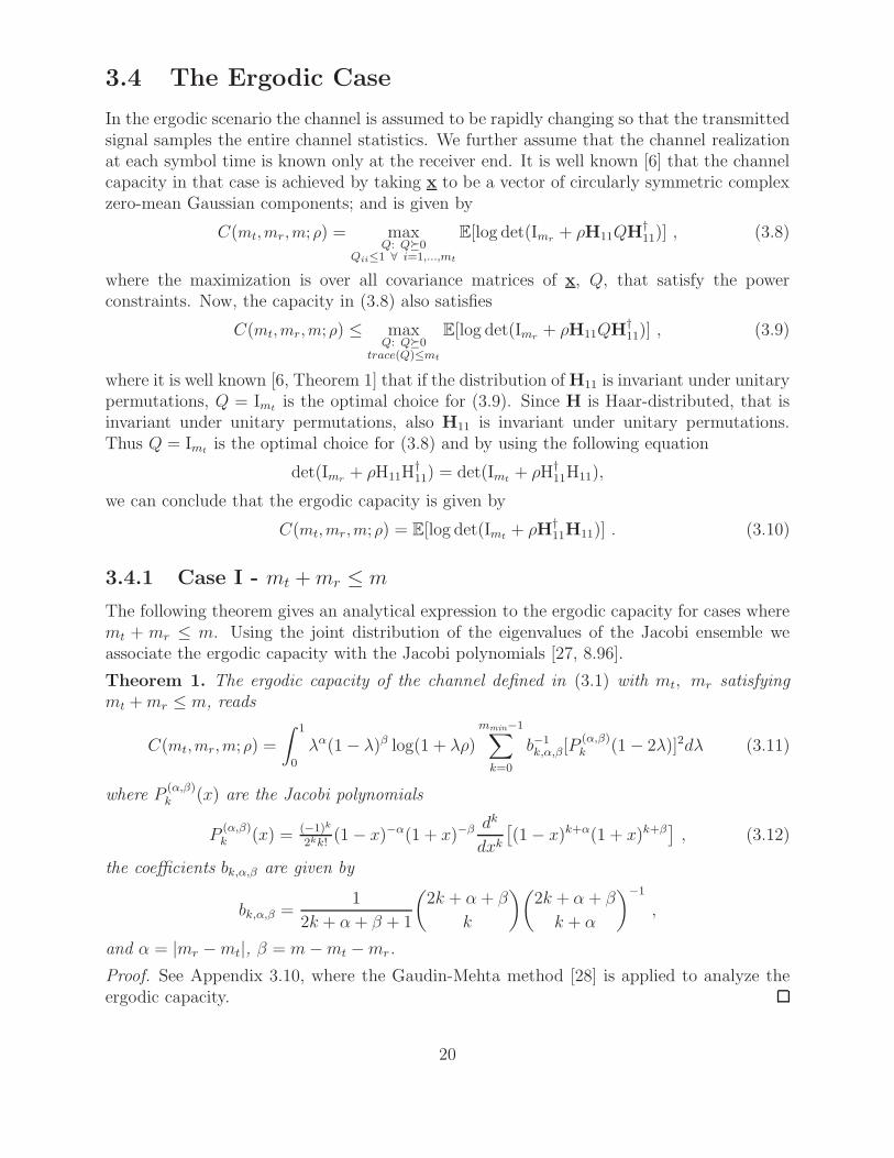
Proof. See Appendix 3.10, where the Gaudin-Mehta method [28] is applied to analyze theergodic capacity.

20

0 10 20 30 40 500

0.5

1

1.5

2

2.5

3

3.5

4

4.5

Nor

mal

ized

Erg

odic

Cap

acity

ρ [dB]

3x3

3x4

2x4

2x3

1x31x4

1x21x1

2x2

4x4

(a)

0 10 20 30 40 500

0.5

1

1.5

2

2.5

Nor

mal

ized

Erg

odic

Cap

acity

ρ [dB]

m=32

m=2

m=4

m=3

m=6

m=8

m=128m=64

m=16

(b)

Figure 3.1: The ergodic capacity, normalized by C(1, 1, 1; ρ) = log(1 + ρ), as a function of ρ.In (a) the number of supported modes is fixed m = 4, various numbers of transmit×receivemodes; in (b) the number of addressed modes is fixed mt = mr = 2, various values ofsupported modes m.


Applying Lemma 1 to the channel capacity given in (3.10) readily results in the followingtheorem.

Theorem 2. The ergodic capacity of the channel defined in (3.1) with mt, mr satisfyingmt +mr > m, reads

C(mt,mr,m; ρ) =(mt +mr −m)C(1, 1, 1; ρ) + C(m−mr,m−mt,m; ρ) , (3.13)

where C(1, 1, 1; ρ) is the SISO channel capacity log(1 + ρ).

Proof. According to (3.10) the ergodic capacity satisfies


11H11)] (3.14)

= E[mt∑

i=1

log(1 + ρλi)] , (3.15)

where λimt

i=1 are the eigenvalues ofH†11H11. According to Lemma 1, mt+mr−m eigenvalues

are 1 and the rest are equal to the m−mr eigenvalues of H22H†22. Applying that into (3.15)

results

C(mt,mr,m; ρ) = (mt +mr −m) log(1 + ρ) + E[log det(Im−mr+ ρH22H

†22))] . (3.16)

21

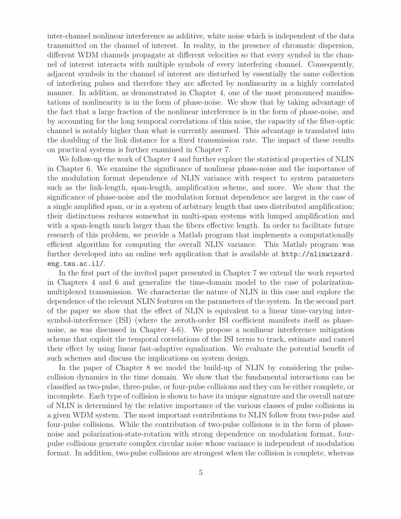
Note that the second term on the right-hand-side of (3.13), C(m−mr,m−mt,m; ρ), isgiven by Theorem 1 and reduces to 0 when mt, or mr is equal to m. Thus, (3.13) suggeststhat for systems with k = mt + mr − m > 0, the ergodic capacity is the sum capacitiesof k unfaded SISO capacities and a Jacobi MIMO channel with m − mr transmit modesand m − mt receive modes. Fig. 3.1a depicts the ergodic capacity as a function of ρ form = 4 and various combinations of mt, mr (note that the ergodic capacity, in our case, issymmetric in mt, mr; thus all combinations are plotted). As is evident from the figure, acapacity equivalent to k SISO channels is guaranteed in all cases. In Fig. 3.1b the ergodiccapacities for mt = mr = 2 and various values of supported modes are plotted. Note thatas m increases, the power loss increases and the ergodic capacity becomes smaller. Unlikethe common practice of expressing the capacity in terms of the received SNR, here thecapacities are presented as a function of ρ. This normalizes the capacity expression to reflectthe capacity loss due to power loss including power leaked into the unobserved modes. Inparticular, this presentation enables to examine the total effect (capacity loss) of increasingm. See further discussion in section 3.8.

3.5 The Non-Ergodic Case

In the non-ergodic scenario the channel matrix is drawn randomly but rather assumed tobe constant within the entire transmission period of each code-frame. The figure of meritin the non-ergodic case is the outage probability defined as the probability that the mutualinformation induced by the channel realization is lower than the rate R at which the link ischosen to operate. Note that we assume that the channel instantiation is unknown at thetransmitter, thus it can not adapt the transmission rate. However, the channel is assumedto be known at the receiver end. By taking an input vector of circularly symmetric complexzero-mean Gaussian variables with covariance matrix Q the mutual information is maximizedand the outage probability can be expressed as

Pout(mt,mr,m;R) = infQ: Q0

Pr[log det(Imr

+ ρH11QH†11) < R

], (3.17)

where the minimization is over all covariance matrices Q satisfying the power constraints.Since the statistics of H11 are invariant under unitary permutations, the optimal choice ofQ, when applying constant per-mode power constraint , is simply the identity matrix. Wenote that when imposing total power constraint , the optimal choice of Q may depend on Rand ρ and in general is unknown, even for the Rayleigh channel. Nevertheless, when ρ ≫ 1the identity matrix is approximately the optimal Q (see section 3.7). Thus, in the followingwe make the simplified assumption that the transmitted covariance matrix is the commonlyused choice Q = Imt

.Now, let the transmission rate be R = r log(1 + ρ) (bps/Hz) and let λ = λimmin

i=1 be theordered non-zeros eigenvalues of H†

11H11; we can write

Pout(mt,mr,m; r log(1 + ρ)) = Pr[log det(Imt

+ ρH†11H11) < R

](3.18)

= Pr[mmin∏

i=1

(1 + ρλi) < (1 + ρ)r], (3.19)

and evaluate this expression by applying the statistics of λ.

22


Using (3.3) we can apply the joint distribution of λ into (3.19) to get

Pout(mt,mr,m; r log(1 + ρ)) = K−1mt,mr,m

∫

B

mmin∏

i=1

λ|mr−mt|i (1− λi)

m−mr−mt

∏

i<j

(λi − λj)2dλ ,

(3.20)

where Kmt,mr ,m is a normalizing factor and B describes the outage event

B =

λ :

mmin∏

i=1

(1 + ρλi) < (1 + ρ)r.

This gives an analytical expression to the outage probability. See Fig. 3.3 and the examplebelow.

Example 1. Suppose mt = 1 and mr, m satisfy m ≥ 1 + mr. In that case the outageprobability is given by

Pout(1,mr,m;R) = K−11,mr ,m

∫ (2R−1)/ρ

0

λmr−1(1− λ)m−mr−1dλ . (3.21)

Thus, we can write

Pout(1,mr,m;R) =B((2R − 1)/ρ;mr, m−mr)

B(1;mr, m−mr), (3.22)

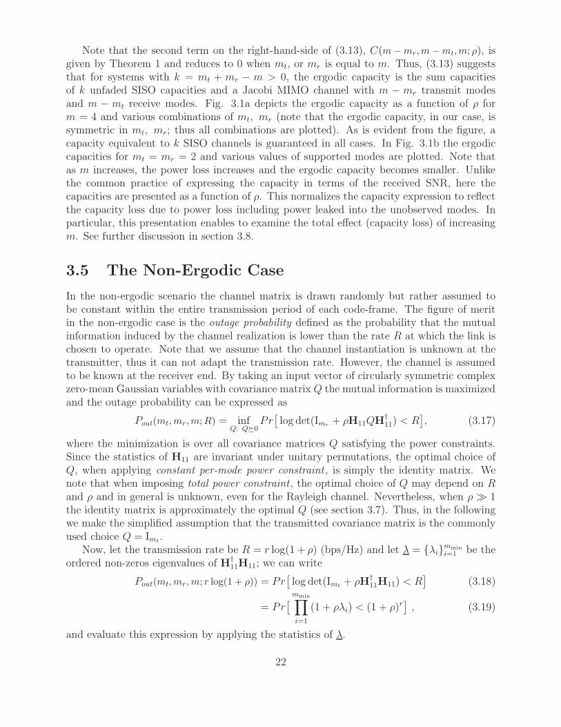
where B(x; a, b) is the incomplete beta function. Hence, to support an outage probabilitysmaller than ǫ, R and ρ have to satisfy

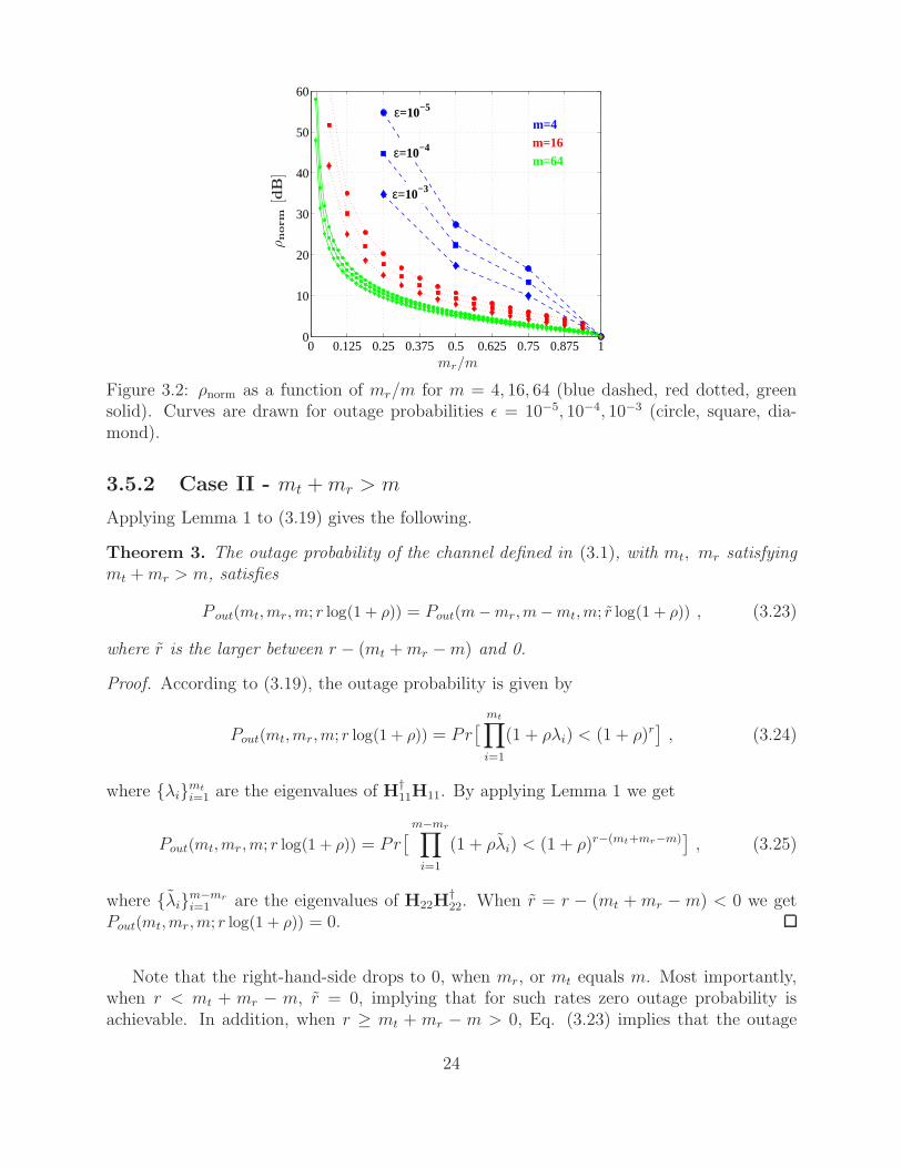
ρ

2R − 1≥ ρnorm = 1/B−1(ǫB(1;mr, m−mr);mr, m−mr) ,

where B−1(x; a, b) is the inverse function of B(x; a, b). ρnorm is the normalized signal-to-noise ratio at the transmitter, is proportional to the received normalized signal-to-noise ratio,and essentially measures the minimal additional power required to support a target rate Rwith outage probability smaller than ǫ (additional power over the minimal required in SISOunfading channel (m = mr)). As ρnorm is smaller one can afford higher data rate or smallerρ (smaller transmission power).In Fig. 3.2 we plot ρnorm as a function of mr/m for various numbers of available modesm and desired outage probabilities ǫ. For fixed m and mr/m, ρnorm increases as ǫ decreases(since more power or lower data rate are needed to achieve smaller outage probability). Forfixed ǫ and m, ρnorm decreases as mr/m increases (since more modes are addressed by thereceiver, therefore the power loss decreases). This is also true as m increases while ǫ andmr/m are fixed (since the diversity at the receiver increases, see Section 3.7). Note that formr/m = 1 there is no power loss and we get ρnorm = 1, that is, the minimal transmissionpower required to support the rate R, for any ǫ, is ρ = 2R − 1.

23

0 0.125 0.25 0.375 0.5 0.625 0.75 0.875 10

10

20

30

40

50

60

ε=10−5

ε=10−4

ε=10−3

m=4m=16m=64

mr/m

ρnorm

[dB]

Figure 3.2: ρnorm as a function of mr/m for m = 4, 16, 64 (blue dashed, red dotted, greensolid). Curves are drawn for outage probabilities ǫ = 10−5, 10−4, 10−3 (circle, square, dia-mond).


Applying Lemma 1 to (3.19) gives the following.

Theorem 3. The outage probability of the channel defined in (3.1), with mt, mr satisfyingmt +mr > m, satisfies

P out(mt,mr,m; r log(1 + ρ)) = Pout(m−mr,m−mt,m; r log(1 + ρ)) , (3.23)

where r is the larger between r − (mt +mr −m) and 0.

Proof. According to (3.19), the outage probability is given by

Pout(mt,mr,m; r log(1 + ρ)) = Pr[ mt∏

i=1

(1 + ρλi) < (1 + ρ)r], (3.24)

where λimt

i=1 are the eigenvalues of H†11H11. By applying Lemma 1 we get

Pout(mt,mr,m; r log(1 + ρ)) = Pr[m−mr∏

i=1

(1 + ρλi) < (1 + ρ)r−(mt+mr−m)], (3.25)

where λim−mr

i=1 are the eigenvalues of H22H†22. When r = r − (mt +mr −m) < 0 we get

Pout(mt,mr,m; r log(1 + ρ)) = 0.

Note that the right-hand-side drops to 0, when mr, or mt equals m. Most importantly,when r < mt + mr − m, r = 0, implying that for such rates zero outage probability isachievable. In addition, when r ≥ mt + mr − m > 0, Eq. (3.23) implies that the outage

24

0 1 2 3 4

10−6

10−4

10−2

100

r=R/log(1+ρ)

Out

age

Pro

babi

lity

1x4 2x4 3x4 4x4

1x2 2x3

2x2 3x31x1

1x3

(a)

0 0.5 1 1.5 2

10−6

10−4

10−2

100

r=R/log(1+ρ)

Out

age

Pro

babi

lity

m=4 m=3m=6m=8m=16

m=32m=64

m=128

m=2

(b)

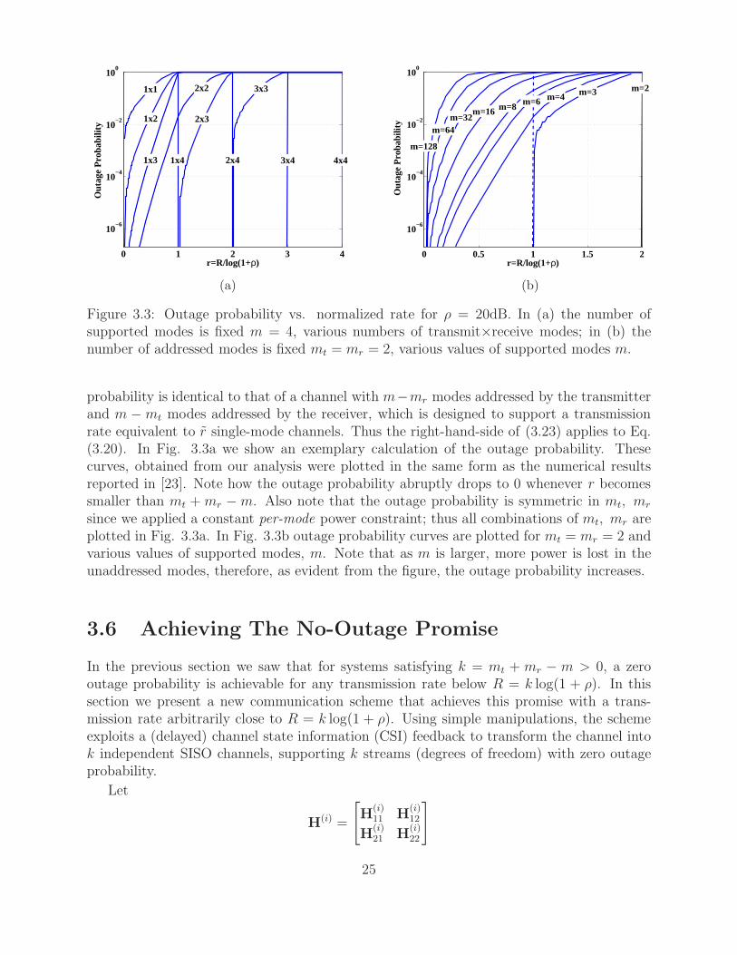
Figure 3.3: Outage probability vs. normalized rate for ρ = 20dB. In (a) the number ofsupported modes is fixed m = 4, various numbers of transmit×receive modes; in (b) thenumber of addressed modes is fixed mt = mr = 2, various values of supported modes m.

probability is identical to that of a channel with m−mr modes addressed by the transmitterand m −mt modes addressed by the receiver, which is designed to support a transmissionrate equivalent to r single-mode channels. Thus the right-hand-side of (3.23) applies to Eq.(3.20). In Fig. 3.3a we show an exemplary calculation of the outage probability. Thesecurves, obtained from our analysis were plotted in the same form as the numerical resultsreported in [23]. Note how the outage probability abruptly drops to 0 whenever r becomessmaller than mt +mr −m. Also note that the outage probability is symmetric in mt, mr

since we applied a constant per-mode power constraint; thus all combinations of mt, mr areplotted in Fig. 3.3a. In Fig. 3.3b outage probability curves are plotted for mt = mr = 2 andvarious values of supported modes, m. Note that as m is larger, more power is lost in theunaddressed modes, therefore, as evident from the figure, the outage probability increases.

3.6 Achieving The No-Outage Promise

In the previous section we saw that for systems satisfying k = mt + mr − m > 0, a zerooutage probability is achievable for any transmission rate below R = k log(1 + ρ). In thissection we present a new communication scheme that achieves this promise with a trans-mission rate arbitrarily close to R = k log(1 + ρ). Using simple manipulations, the schemeexploits a (delayed) channel state information (CSI) feedback to transform the channel intok independent SISO channels, supporting k streams (degrees of freedom) with zero outageprobability.

Let

H(i) =

[H

(i)11 H

(i)12

H(i)21 H

(i)22

]

25

be the unitary matrix realization at channel use i and let

y(i) =√ρH

(i)11x

(i) + z(i)

be the received signal. We assume a perfect knowledge of H(i)11 at the receiver and a noiseless

CSI feedback with a delay of a single channel use. Since H(i) is unitary, a matrix H(i)21 can

be computed to complete H(i)11 into orthonormal columns. Therefore, we shall assume that

the receiver noiselessly communicates this computed H(i)21 to the transmitter. Nevertheless,

note that for mt +mr −m > 1 and certain matrix instantiations, the computed H(i)21 is not

unique and can be chosen wisely (see Remark 4).Now, let the transmitter excites the following signal from the addressed modes at each

channel use i = 1, . . . , n

x(i) =

x(i)1...

x(i)mt+mr−m

H(i−1)21 x(i−1)

.

That is, the transmitter conveysmt+mr−m new information bearing symbols andH(i−1)21 x(i−1),

a linear combination of the signal that was transmitted in the previous channel use (x(0) isa vector of zeros). Note that H is unitary, thus the power constraint is left satisfied.

We shall now assume that after the last signal y(n) is received, the receiver gets as a sideinformation the following noisy measures

ysi=

√ρH

(n)21 x

(n) + zsi , (3.26)

where the components of zsi are i.i.d. CN (0, 1). Thus the receiver can linearly combine y(n)

and ysiin the following manner

y(n) =[H

(n)†11 H

(n)†21

] [[c] y(n)

ysi

](3.27)

to yield

y(n) =√ρx(n) + z (3.28)

where the entries of z are i.i.d. CN (0, 1). We remind that the first mt + mr − m entries

of x(n) are new information bearing symbols and the last entries are equal to H(n−1)21 x(n−1).

Thus, the last m−mr entries of y(n), denoted y, satisfy

y =√ρH

(n−1)21 x(n−1) + z .

where z are the last m−mr entries of z. Again, the receiver can linearly combine y(n−1) andy as

y(n−1) =[H

(n−1)†11 H

(n−1)†21

] [[c] y(n−1)

y

](3.29)

26

to yield measures of x(n−1) as in Eq. (3.28). Repeating this procedure for i = n − 1 → 1results in mt +mr −m independent streams of measures

y(1)1...

y(1)mt+mr−m

, . . . ,

y(n)1...

y(n)mt+mr−m

.

The scheme above is feasible if the side information after channel use n is being conveyedby the transmitter through a neglectable number of channel uses (with respect to n, seeRemark 3). In that case the receiver can construct mt+mr−m independent SISO channels,each with signal-to-noise ratio ρ. Thus the scheme supports a rate arbitrarily close (as nis larger) to (mt +mr −m) log(1 + ρ) with zero outage probability. Note that the schemeessentially completes the singular values of the channel to 1. This is feasible since m−mr <mt, thus at each channel use the transmitter can transmit H

(i−1)21 x(i−1), a signal of m −mr

entries, and new symbols.The scheme presented above can be easily expanded to the case where the feedback delay

is l channel uses. In that case the transmitter conveys at each channel use mt + mr − mnew information bearing symbols and H

(i−l)21 x(i−l), a linear combination of the signal that

was transmitted l channel uses before. After channel use n, the transmitter would have toconvey l noisy measures of the last l signals, so that the receiver could construct mt+mr−mindependent SISO channels. This can be done in a fixed number of channel uses (see Remark3), thus as n is larger, the transmission rate of the scheme approaches (mt+mr−m) log(1+ρ).

Remark 1 (Outdated feedback). Our scheme exploits a noiseless CSI feedback system tocommunicate a (possibly) outdated information - the channel realization in previous channeluses. Thus, the feedback is not required to be fast, that is, no limitations on the delay timel. However, if l is smaller than the coherence time of the channel, the feedback may carryinformation about the current channel realization. Thus, the transmitter can exploit theup-to-date feedback to use more efficient schemes. Nevertheless, for systems with a longdelay time (e.g., relatively long distance optical fibers), the channel can be regarded as non-ergodic with an outdated feedback. In these cases our scheme efficiently achieves zero outageprobability.

Remark 2 (Simple decoding). The scheme linearly process the received signals to constructmt +mr −m independent streams of measures, each with signal-to-noise ρ. This allows thedecoding stage to be simple, where a SISO channel decoder can be used, removing the needfor further MIMO signal processing.

Remark 3 (Side information measures). For a feedback with a delay of l channel uses, the

transmitter has to convey H(i)21x

(i), for each i = n− (l− 1), . . . , n, such that the receiver canextracted a vector of noisy measures with signal-to-noise ratio that is not smaller than ρ. Thisis feasible with a finite number of channel uses. For example, the repetition scheme can beused to convey these measures (see Section 3.7 Example 2). Suppose each H

(i)21x

(i) is conveyedto the receiver within Nsi channel uses (e.g., for the repetition scheme Nsi = mt(m−mr)). Bytaking large enough n (with respect to l·Nsi) one can approach the rate (mt+mr−m) log(1+ρ).

27

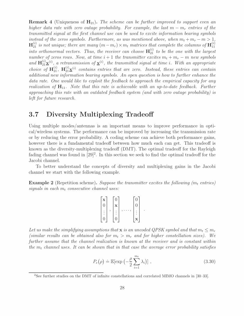
Remark 4 (Uniqueness of H21). The scheme can be further improved to support even anhigher data rate with zero outage probability. For example, the last m − mr entries of thetransmitted signal at the first channel use can be used to excite information bearing symbolsinstead of the zeros symbols. Furthermore, as was mentioned above, when mt +mr −m > 1,H

(i)21 is not unique; there are many (m−mr)×mt matrices that complete the columns of H

(i)11

into orthonormal vectors. Thus, the receiver can choose H(i)21 to be the one with the largest

number of zeros rows. Now, at time i+ 1 the transmitter excites mt +mr −m new symbolsand H

(i)21x

(i), a retransmission of x(i), the transmitted signal at time i. With an appropriate

choice of H(i)21 , H

(i)21x

(i) contains entries that are zero. Instead, these entries can containadditional new information bearing symbols. An open question is how to further enhance thedata rate. One would like to exploit the feedback to approach the empirical capacity for anyrealization of H11. Note that this rate is achievable with an up-to-date feedback. Furtherapproaching this rate with an outdated feedback system (and with zero outage probability) isleft for future research.

3.7 Diversity Multiplexing Tradeoff

Using multiple modes/antennas is an important means to improve performance in opti-cal/wireless systems. The performance can be improved by increasing the transmission rateor by reducing the error probability. A coding scheme can achieve both performance gains,however there is a fundamental tradeoff between how much each can get. This tradeoff isknown as the diversity-multiplexing tradeoff (DMT). The optimal tradeoff for the Rayleighfading channel was found in [29]2. In this section we seek to find the optimal tradeoff for theJacobi channel.

To better understand the concepts of diversity and multiplexing gains in the Jacobichannel we start with the following example.

Example 2 (Repetition scheme). Suppose the transmitter excites the following (mt entries)signals in each mt consecutive channel uses:

x

0...0

,

0x...0

, . . . ,

00...x

.

Let us make the simplifying assumptions that x is an uncoded QPSK symbol and that mt ≤ mr

(similar results can be obtained also for mt > mr and for higher constellation sizes). Wefurther assume that the channel realization is known at the receiver and is constant withinthe mt channel uses. It can be shown that in that case the average error probability satisfies

Pe

(ρ) .= E[exp

(−ρ2

mt∑

i=1

λi)] , (3.30)

2See further studies on the DMT of infinite constellations and correlated MIMO channels in [30–33].

28

where the expectation is over λimt

i=1, the eigenvalues of H†11H11. Here and throughout the

rest of the paper we use.= to denote exponential equality, i.e., f(ρ)

.= ρd denotes

limρ→∞

log f(ρ)

log ρ= d . (3.31)

Now, for mt +mr ≤ m, we can apply the joint distribution of the unordered eigenvalues ofa Jacobi matrix J (mr, m−mr, mt), to write

Pe

(ρ) .=

K−1mt,mr,m

mt!

∫ 1

0

. . .

∫ 1

0

mt∏

i=1

λmr−mt

i (1− λi)m−mr−mte−

ρ2λi

∏

i<j

(λj − λi)2

mt∏

i=1

dλi . (3.32)

Note that the term ∏

1≤i<j≤mt

(λj − λi)

is the determinant of the Vandermonde matrix

1 . . . 1λ1 . . . λmt

......

λmt−11 . . . λmt−1

mt

.

Thus we can write

∏

1≤i<j≤mt

(λj − λi)2 =

∑

σ1,σ2∈Smt

(−1)sgn(σ1)+sgn(σ2)

mt∏

i=1

λσ1(i)+σ2(i)−2i , (3.33)

where Smtis the set of all permutations of 1, . . . , mt and sgn(σ) denotes the signature of

the permutation σ. Applying (3.33) into (3.32) results

Pe

(ρ) .=

K−1mt,mr,m

mt!

∑

σ1,σ2∈Smt

(−1)sgn(σ1)+sgn(σ2)mt∏

i=1

∫ 1

0

λmr−mt+σ1(i)+σ2(i)−2i ×

× (1− λi)m−(mr+mt)e−

ρ2λidλi . (3.34)

It can be further shown that the right-hand-side of above is dominated (for large ρ) by thefollowing term

K−1mt,mr,m

mt!

∑

σ1,σ2∈Smt


mt∏

i=1

(mr −mt + σ1(i) + σ2(i)− 2)!(ρ2)−(mr−mt+σ1(i)+σ2(i)−1) .

(3.35)

Thus, for mt +mr ≤ m, the average error probability satisfies

Pe

(ρ) .= ρ−

∑mti=1

(mr−mt+2i−1) (3.36).= ρ−mrmt . (3.37)

29

For mt +mr > m, by applying Lemma 1 into (3.30) we get

Pe

(ρ) .= e−

ρ(mt+mr−m)2 E[exp

(−ρ

2

m−mr∑

i=1

λi)] ,

where λim−mr

i=1 are the eigenvalues of H22H†22. Thus, we can conclude that the error prob-

ability of the repetition scheme satisfies

Pe

(ρ) .=

ρ−mrmt , mt +mr ≤ m

e−ρ(mt+mr−m)

2 ρ−(m−mt)(m−mr) , mt +mr > m .(3.38)

0 5 10 15

10−4

10−2

100

ρ[dB]

Err

or P

roba

bilit

y

mt+m

r≤ m

mt+m

r>m

α⋅ρ−mtm

r

1x1

1x2

1x3

1x42x32x43x33x44x42x2

Figure 3.4: The average error probability of the repetition scheme vs. ρ, for fixed numberof supported modes m = 4 and various numbers of transmit×receive modes. The errorprobability curves are depict in solid lines for systems satisfying mt+mr ≤ m and in dottedlines for systems satisfying mt + mr > m. The dashed lines are given to emphasize thedecaying order of the non-exponentially decaying curves.

In Fig. 3.4 we present the average error probability vs. ρ for m = 4 and various combi-nations of mt, mr (the error probability is symmetric in mt, mr, thus all combinations ofmt, mr are plotted). Note the decaying order of the curves and how they turn exponentiallydecaying when mt +mr > m.

Eq. (3.38) implies that when using mt transmit and mr receive modes, where mt+mr ≤m, the exponent of the dominant term in the average error probability is −mrmt. Comparingto a system with a single transmit and a single receive mode, the decaying order of the averageerror probability is improved by a factor of mrmt. This gain is termed diversity gain. Whenenough modes are being addressed by the transmitter and the receiver to satisfymt+mr > m,we get an average error probability that exponentially decays with ρ; that is, an unboundeddiversity gain. Thus, as more modes are being addressed, the diversity gain of the repetitionscheme is greater. Since the total transmitted power is spread over all m available modes,

30

addressing only some modes at the receiver results in a power loss. As the number of thesemodes is larger, the probability for a substantial power loss is smaller; hence, smaller errorprobability. As the signal is transmitted from more modes, the average power in each receivemode is larger since the propagation paths are orthogonal. This is in analogy to the Rayleighchannel where as the signal passes through more (independent) faded paths, the decayingorder of the error probability increases. However, it turns out that in the Jacobi channelthere is a transition threshold in which enough modes are being addressed to ensure a certainreceived power. This results in an exponentially decaying error probability for certain rates.

Now, using multiple modes can also improve the data rate of the system. In the exampleabove the rate is fixed, R(ρ) = 1/mt (bps/Hz) for any ρ. Increasing the data rate withρ to support a rate of R(ρ) = r log ρ (bps/Hz) for some 0 < r < 1/mt, can be achievedby increasing the constellation size of the transmitted signal. In that case the data rateis improved by a factor of r comparing to a system with a single transmit and a singlereceive mode. This gain is termed multiplexing gain 3. By increasing the constellation size,however, the minimum distance between the constellation points decreases, resulting an errorprobability with a smaller decaying order; that is, a smaller diversity gain. Thus, there is atradeoff between diversity and multiplexing gains.

We now turn to analyze the DMT in the Jacobi model. To that end, we formalize theconcepts of diversity gain and multiplexing gain by quoting some definitions from [29] 4.

Definition 4. Let a scheme be a family of codesC(ρ)

of block length l, one at each ρ

level. Let R(ρ) (bps/Hz) be the rate of the code C(ρ). A schemeC(ρ)

is said to achieve

spatial multiplexing gain r and diversity gain d if the data rate satisfies

limρ→∞

R(ρ)

log ρ= r

and the average error probability satisfies

limρ→∞

Pe(ρ)

log ρ= −d .

For each r, define d∗(r) to be the supremum of the diversity advantage achieved over allschemes.


The following Theorem provides the optimal DMT of a Jacobi channel with mt, mr andm satisfying mt +mr ≤ m. In [29] it was shown that the average error probability in thehigh SNR regime (large ρ) is dominated by the outage probability. Furthermore, the outageprobability for a transmission rate R = r log(1 + ρ), where r is integer, is dominated bythe probability that r singular values of the channel are 1 and the other approach zero. We

3The multiplexing gain in the given example is 0.4Note that in [29] the definitions in 4 were made with respect to the average signal-to-noise ratio at each

receive mode, denoted ρ. However, since ρ = ρE[ tr(H11QH†11)]/mr, where Q is the transmitted covariance

matrix, we can write limρ→∞ log ρ = limρ→∞ log ρ . Hence the definitions in 4 coincide with those in [29].

31

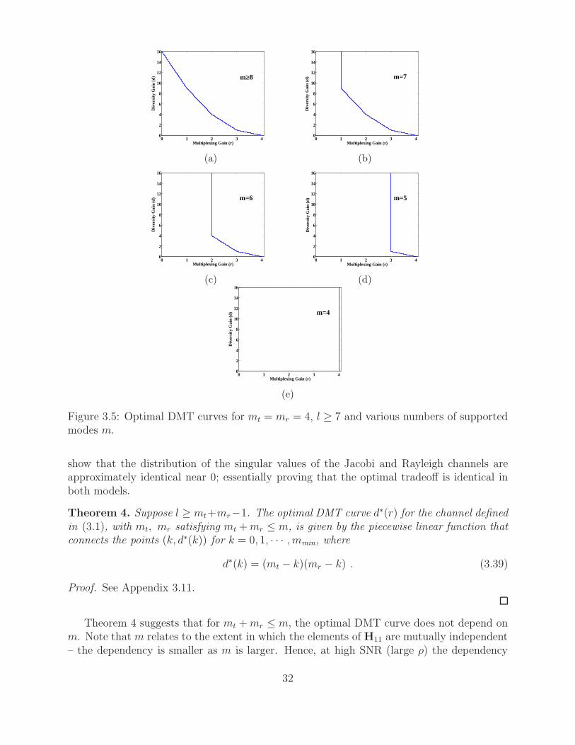
0 1 2 3 40

2

4

6

8

10

12

14

16

Multiplexing Gain (r)

Div

ersi

ty G

ain

(d) m≥8

(a)

0 1 2 3 40

2

4

6

8

10

12

14

16


Div

ersi

ty G

ain

(d) m=7

(b)

0 1 2 3 40

2

4

6

8

10

12

14

16


Div

ersi

ty G

ain

(d) m=6

(c)

0 1 2 3 40

2

4

6

8

10

12

14

16


Div

ersi

ty G

ain

(d) m=5

(d)

0 1 2 3 40

2

4

6

8

10

12

14

16


Div

ersi

ty G

ain

(d) m=4

(e)

Figure 3.5: Optimal DMT curves for mt = mr = 4, l ≥ 7 and various numbers of supportedmodes m.

show that the distribution of the singular values of the Jacobi and Rayleigh channels areapproximately identical near 0; essentially proving that the optimal tradeoff is identical inboth models.

Theorem 4. Suppose l ≥ mt+mr−1. The optimal DMT curve d∗(r) for the channel definedin (3.1), with mt, mr satisfying mt +mr ≤ m, is given by the piecewise linear function thatconnects the points (k, d∗(k)) for k = 0, 1, · · · , mmin, where

d∗(k) = (mt − k)(mr − k) . (3.39)

Proof. See Appendix 3.11.

Theorem 4 suggests that for mt +mr ≤ m, the optimal DMT curve does not depend onm. Note that m relates to the extent in which the elements of H11 are mutually independent– the dependency is smaller as m is larger. Hence, at high SNR (large ρ) the dependency

32

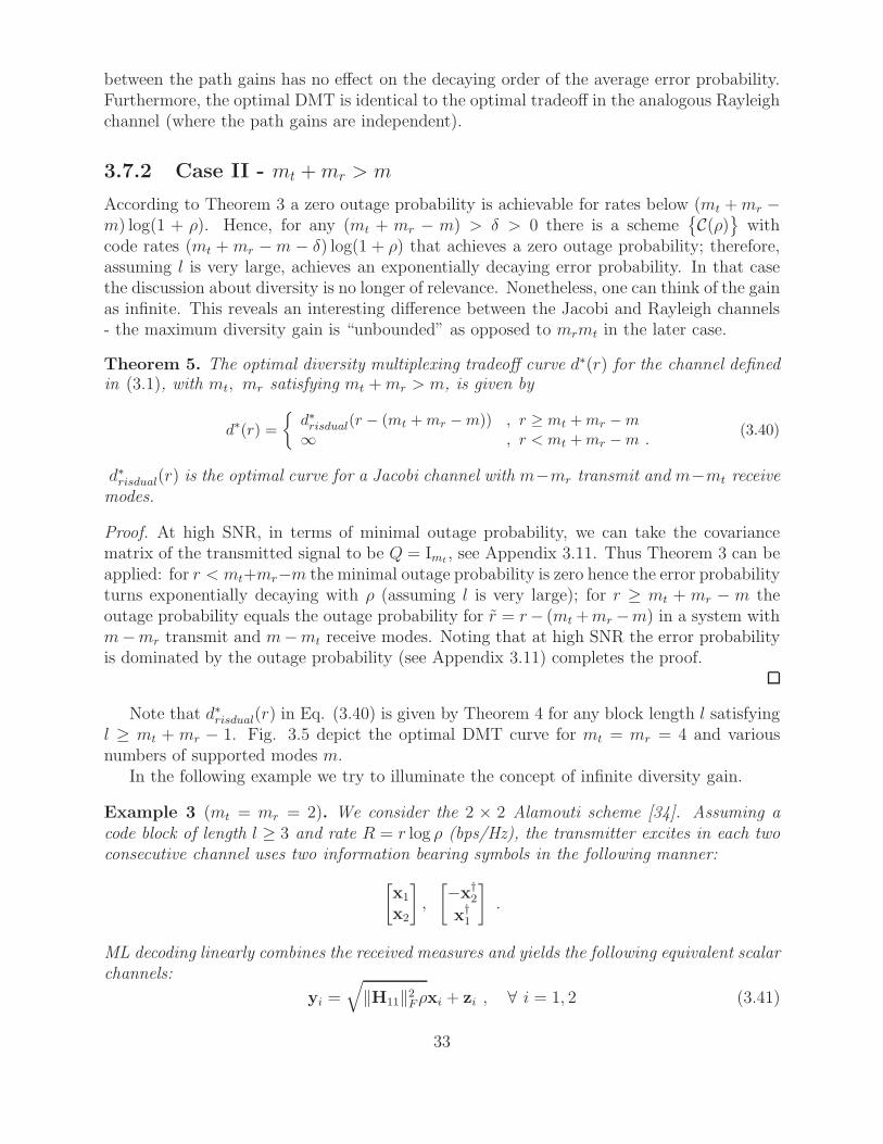
between the path gains has no effect on the decaying order of the average error probability.Furthermore, the optimal DMT is identical to the optimal tradeoff in the analogous Rayleighchannel (where the path gains are independent).


According to Theorem 3 a zero outage probability is achievable for rates below (mt +mr −m) log(1 + ρ). Hence, for any (mt + mr − m) > δ > 0 there is a scheme

C(ρ)

with

code rates (mt +mr −m − δ) log(1 + ρ) that achieves a zero outage probability; therefore,assuming l is very large, achieves an exponentially decaying error probability. In that casethe discussion about diversity is no longer of relevance. Nonetheless, one can think of the gainas infinite. This reveals an interesting difference between the Jacobi and Rayleigh channels- the maximum diversity gain is “unbounded” as opposed to mrmt in the later case.

Theorem 5. The optimal diversity multiplexing tradeoff curve d∗(r) for the channel definedin (3.1), with mt, mr satisfying mt +mr > m, is given by

d∗(r) =

d∗risdual(r − (mt +mr −m)) , r ≥ mt +mr −m∞ , r < mt +mr −m .

(3.40)

d∗risdual(r) is the optimal curve for a Jacobi channel with m−mr transmit and m−mt receivemodes.

Proof. At high SNR, in terms of minimal outage probability, we can take the covariancematrix of the transmitted signal to be Q = Imt

, see Appendix 3.11. Thus Theorem 3 can beapplied: for r < mt+mr−m the minimal outage probability is zero hence the error probabilityturns exponentially decaying with ρ (assuming l is very large); for r ≥ mt + mr − m theoutage probability equals the outage probability for r = r− (mt +mr −m) in a system withm−mr transmit and m−mt receive modes. Noting that at high SNR the error probabilityis dominated by the outage probability (see Appendix 3.11) completes the proof.

Note that d∗risdual(r) in Eq. (3.40) is given by Theorem 4 for any block length l satisfyingl ≥ mt + mr − 1. Fig. 3.5 depict the optimal DMT curve for mt = mr = 4 and variousnumbers of supported modes m.

In the following example we try to illuminate the concept of infinite diversity gain.

Example 3 (mt = mr = 2). We consider the 2 × 2 Alamouti scheme [34]. Assuming acode block of length l ≥ 3 and rate R = r log ρ (bps/Hz), the transmitter excites in each twoconsecutive channel uses two information bearing symbols in the following manner:

[x1

x2

],

[−x

†2

x†1

].

ML decoding linearly combines the received measures and yields the following equivalent scalarchannels:

yi =√

‖H11‖2Fρxi + zi , ∀ i = 1, 2 (3.41)

33

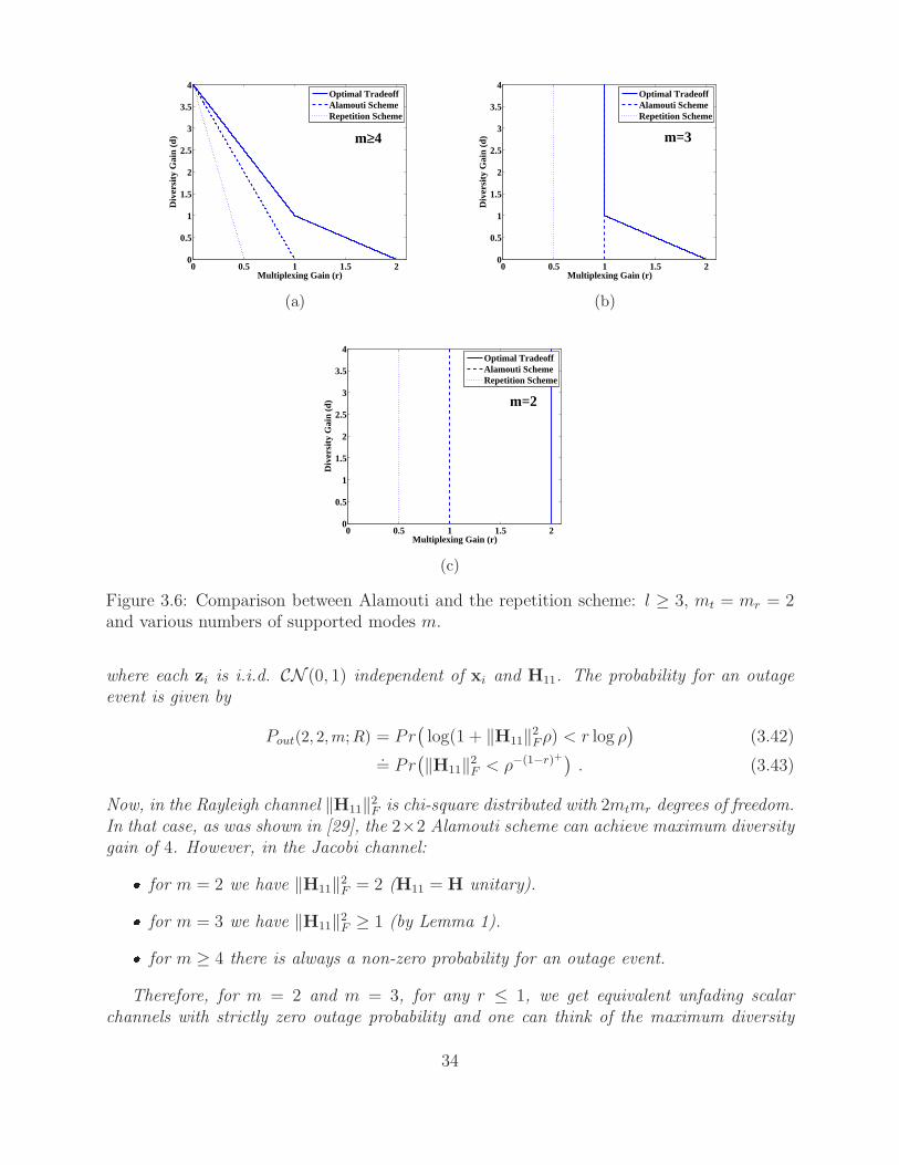
0 0.5 1 1.5 20

0.5

1

1.5

2

2.5

3

3.5

4


Div

ersi

ty G

ain

(d)

Optimal TradeoffAlamouti SchemeRepetition Scheme

m≥4

(a)

0 0.5 1 1.5 20

0.5

1

1.5

2

2.5

3

3.5

4


Div

ersi

ty G

ain

(d)


m=3

(b)

0 0.5 1 1.5 20

0.5

1

1.5

2

2.5

3

3.5

4


Div

ersi

ty G

ain

(d)


m=2

(c)

Figure 3.6: Comparison between Alamouti and the repetition scheme: l ≥ 3, mt = mr = 2and various numbers of supported modes m.

where each zi is i.i.d. CN (0, 1) independent of xi and H11. The probability for an outageevent is given by

Pout(2, 2,m;R) = Pr(log(1 + ‖H11‖2Fρ) < r log ρ

)(3.42)

.= Pr

(‖H11‖2F < ρ−(1−r)+

). (3.43)

Now, in the Rayleigh channel ‖H11‖2F is chi-square distributed with 2mtmr degrees of freedom.In that case, as was shown in [29], the 2×2 Alamouti scheme can achieve maximum diversitygain of 4. However, in the Jacobi channel:

for m = 2 we have ‖H11‖2F = 2 (H11 = H unitary).

for m = 3 we have ‖H11‖2F ≥ 1 (by Lemma 1).

for m ≥ 4 there is always a non-zero probability for an outage event.

Therefore, for m = 2 and m = 3, for any r ≤ 1, we get equivalent unfading scalarchannels with strictly zero outage probability and one can think of the maximum diversity

34

gain as infinite. For m ≥ 4 it can be shown that the maximum diversity gain is 4 and theDMT curve linearly connects the points (1, 0) and (0, 4).

In Example 2 we saw that for multiplexing gain r = 0 the repetition scheme achievesa diversity gain of mrmt for systems satisfying mt + mr ≤ m and an unbounded gain forsystems satisfying mt+mr > m. Thus, for m ≥ 4 the maximum diversity gain of this schemeis 4 and it can be shown that the DMT curve linearly connects the points (1/2, 0) and (0, 4).For m = 2 and m = 3 we get an unbounded diversity gain for any multiplexing gain belowr = 1/2.

In Fig. 3.6 we compare these DMT curves to the optimal curves. Note that for m = 3the Alamouti scheme achieves the optimal DMT for r = 1.

3.8 Relation To The Rayleigh Model

The Jacobi fading model is defined by the transfer matrix H11, a truncated mr ×mt versionof a Haar distributed m × m unitary matrix. We shall now examine the case where m isvery large with respect to mt and mr.

Assuming mt ≤ mr and mt + mr ≤ m, the statistics of the squared singular values ofthe Jacobi channel model follow the law of the Jacobi ensemble J (mr, m − mr, mt). Thisensemble can be constructed as

G†1G1(G

†1G1 +G

†2G2)

−1 , (3.44)

where G1 and G2 are mr×mt and (m−mr)×mt independent Gaussian matrices. Thus, thesquared singular values of H11 share the same distribution with the eigenvalues of (3.44).Intuitively, in terms of the singularity statistics, the Jacobi channel can be viewed as anmr ×mt sub-channel of an m×mt normalized Gaussian channel. Furthermore, for m≫ mr

we have

G†1G1(G

†1G1 +G

†2G2)

−1 = G†1G1(

[G1

G2

]† [G1

G2

])−1 (3.45)

≈ G†1G1(mE[gg†])−1 (3.46)

= 1mG

†1G1 , (3.47)

where in (3.45) we applied the law of large numbers (g is a vector of mt independent com-ponents, each distributed CN (0, 1)). In the same manner, for mt > mr, mt +mr ≤ m andm≫ mt the squared singular values of the Jacobi channel share the same distribution withthe following ensemble of random matrices

G1G†1(G1G

†1 +G2G

†2)

−1 ≈ 1mG1G

†1 . (3.48)

This allows us to conclude that up to a normalizing factor the Jacobi model approaches(with m) the Rayleigh model.

The discussion above provides an “intuitive” proof, using the law of large numbers, to thefact that the Wishart ensemble approaches the Jacobi ensemble as m → ∞. However, thisresult can be proved rigorously and is well known in randommatrix theory. The proof is based

35

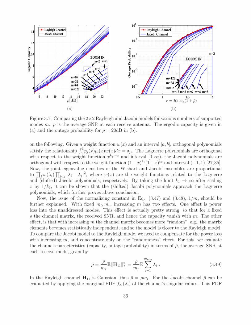
6 8 10 12 14 16 18 20 22

4

6

8

10

12

14E

rgo

dic

Ca

pa

city

Rayleigh ChannelJacobi Channel

16.5 17 17.5 18

10

10.5

11

m=8m=6

m=4

m=2

m=32

m=128m=64

m=3

m=16

ZOOM IN

ρ[dB]

(a)

0.5 1 1.5 2

10−4

10−3

10−2

10−1

100

Ou

tag

e P

rob

ab

ility

Rayleigh ChannelJacobi Channel

1 1.1 1.2

10−2

ZOOM INm=2

m=128m=64m=32

m=6m=8 m=4 m=3m=16

r = R/ log(1 + ρ)

(b)

Figure 3.7: Comparing the 2×2 Rayleigh and Jacobi models for various numbers of supportedmodes m. ρ is the average SNR at each receive antenna. The ergodic capacity is given in(a) and the outage probability for ρ = 20dB in (b).

on the following. Given a weight function w(x) and an interval [a, b], orthogonal polynomials

satisfy the relationship∫ b

apj(x)pi(x)w(x)dx = δji. The Laguerre polynomials are orthogonal

with respect to the weight function xke−x and interval [0,∞), the Jacobi polynomials areorthogonal with respect to the weight function (1−x)k1(1+x)k2 and interval (−1, 1) [27,35].Now, the joint eigenvalue densities of the Wishart and Jacobi ensembles are proportionalto∏

i w(λi)∏

i<j |λi − λj|2, where w(x) are the weight functions related to the Laguerreand (shifted) Jacobi polynomials, respectively. By taking the limit k1 → ∞ after scalingx by 1/k1, it can be shown that the (shifted) Jacobi polynomials approach the Laguerrepolynomials, which further proves above conclusion.

Now, the issue of the normalizing constant in Eq. (3.47) and (3.48), 1/m, should befurther explained. With fixed mt, mr, increasing m has two effects. One effect is powerloss into the unaddressed modes. This effect is actually pretty strong, so that for a fixedρ the channel matrix, the received SNR, and hence the capacity vanish with m. The othereffect, is that with increasing m the channel matrix becomes more “random”, e.g., the matrixelements becomes statistically independent, and so the model is closer to the Rayleigh model.To compare the Jacobi model to the Rayleigh mode, we need to compensate for the power losswith increasing m, and concentrate only on the “randomness” effect. For this, we evaluatethe channel characteristics (capacity, outage probability) in terms of ρ, the average SNR ateach receive mode, given by

ρ =ρ

mr

E‖H11‖2F =ρ

mr

E

mmin∑

i=1

λi . (3.49)

In the Rayleigh channel H11 is Gaussian, thus ρ = ρmt. For the Jacobi channel ρ can beevaluated by applying the marginal PDF fλi

(λi) of the channel’s singular values. This PDF

36

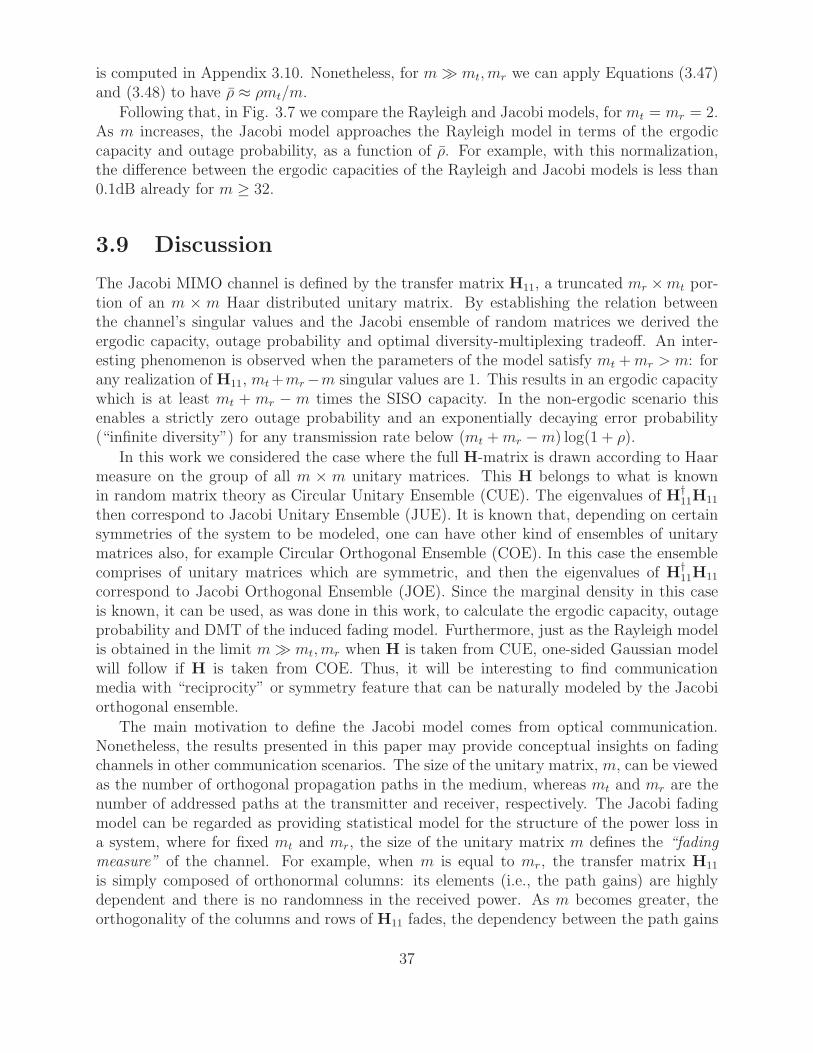
is computed in Appendix 3.10. Nonetheless, for m≫ mt, mr we can apply Equations (3.47)and (3.48) to have ρ ≈ ρmt/m.

Following that, in Fig. 3.7 we compare the Rayleigh and Jacobi models, formt = mr = 2.As m increases, the Jacobi model approaches the Rayleigh model in terms of the ergodiccapacity and outage probability, as a function of ρ. For example, with this normalization,the difference between the ergodic capacities of the Rayleigh and Jacobi models is less than0.1dB already for m ≥ 32.

3.9 Discussion

The Jacobi MIMO channel is defined by the transfer matrix H11, a truncated mr ×mt por-tion of an m × m Haar distributed unitary matrix. By establishing the relation betweenthe channel’s singular values and the Jacobi ensemble of random matrices we derived theergodic capacity, outage probability and optimal diversity-multiplexing tradeoff. An inter-esting phenomenon is observed when the parameters of the model satisfy mt +mr > m: forany realization of H11, mt+mr−m singular values are 1. This results in an ergodic capacitywhich is at least mt + mr − m times the SISO capacity. In the non-ergodic scenario thisenables a strictly zero outage probability and an exponentially decaying error probability(“infinite diversity”) for any transmission rate below (mt +mr −m) log(1 + ρ).

In this work we considered the case where the full H-matrix is drawn according to Haarmeasure on the group of all m × m unitary matrices. This H belongs to what is knownin random matrix theory as Circular Unitary Ensemble (CUE). The eigenvalues of H†

11H11

then correspond to Jacobi Unitary Ensemble (JUE). It is known that, depending on certainsymmetries of the system to be modeled, one can have other kind of ensembles of unitarymatrices also, for example Circular Orthogonal Ensemble (COE). In this case the ensemblecomprises of unitary matrices which are symmetric, and then the eigenvalues of H†

11H11

correspond to Jacobi Orthogonal Ensemble (JOE). Since the marginal density in this caseis known, it can be used, as was done in this work, to calculate the ergodic capacity, outageprobability and DMT of the induced fading model. Furthermore, just as the Rayleigh modelis obtained in the limit m≫ mt, mr when H is taken from CUE, one-sided Gaussian modelwill follow if H is taken from COE. Thus, it will be interesting to find communicationmedia with “reciprocity” or symmetry feature that can be naturally modeled by the Jacobiorthogonal ensemble.

The main motivation to define the Jacobi model comes from optical communication.Nonetheless, the results presented in this paper may provide conceptual insights on fadingchannels in other communication scenarios. The size of the unitary matrix, m, can be viewedas the number of orthogonal propagation paths in the medium, whereas mt and mr are thenumber of addressed paths at the transmitter and receiver, respectively. The Jacobi fadingmodel can be regarded as providing statistical model for the structure of the power loss ina system, where for fixed mt and mr, the size of the unitary matrix m defines the “fadingmeasure” of the channel. For example, when m is equal to mr, the transfer matrix H11

is simply composed of orthonormal columns: its elements (i.e., the path gains) are highlydependent and there is no randomness in the received power. As m becomes greater, theorthogonality of the columns and rows of H11 fades, the dependency between the path gains

37

becomes weaker and the power loss in the unaddressed receive outputs increases. Indeed,when m is very large with respect tomt andmr, with proper normalization that compensatesfor the average power loss, the Jacobi fading model approaches to the Rayleigh model. TheJacobi model, thus, introduces new concepts in fading channels, providing a degree of freedomto scale the model from a unitary channel up to the Rayleigh channel.

Acknowledgement

We wish to thank Amir Dembo and Yair Yona for interesting discussions on Lemma 1.

3.10 Appendix: Proof of Theorem 1

The Gaudin-Mehta method [28] is used here for proving Theorem 1.According to (3.10), the ergodic capacity satisfies


11H11)] (3.50)

= E[

mt∑

i=1

log(1 + ρλi)] (3.51)

where we denote by λimt

i=1 the eigenvalues of H†11H11. To simplify notations let us assume

mt ≤ mr (one can simply replace mt with mr to obtain the proof for mt > mr). Thus, wecan write

C(mt,mr,m; ρ) = mtE[log(1 + ρλ1)]. (3.52)

Now, the joint distribution of the ordered eigenvalues fλ(λ1, . . . , λmt) is given by (3.3). The

joint distribution of the unordered eigenvalues equals

1mt!fλ(λ1, . . . , λmt

) ,

thus we can compute the density of λ1 by integrating out λimt

i=2, that is

fλ1(λ1) =

∫ 1

0

. . .

∫ 1

0

1mt!fλ(λ1, . . . , λmt

)

mt∏

i=2

dλi . (3.53)

By takingλi =

12(1− λi) (3.54)

we can write

fλ1(λ1) =

∫ 1

−1

. . .

∫ 1

−1

fλ(λ1, . . . , λmt)

mt∏

i=2

dλi , (3.55)

where

fλ(λ1, . . . , λmt) = K−1

mt,mr ,m

mt∏

i=1

(1− λi)α(1 + λi)

β∏

i<j

(λi − λj)2 , (3.56)

38

and α = mr −mt, β = m−mr −mt. Now, the term

∏

1≤i<j≤mt

(λi − λj)

is the determinant of the Vandermonde matrix

1 . . . 1

λ1 . . . λmt

......

λmt−11 . . . λmt−1

mt

. (3.57)

With row operations we can transform (3.57) into the following matrix

P

(α,β)0 (λ1) . . . P

(α,β)0 (λmt

)...

...

P(α,β)mt−1(λ1) . . . P

(α,β)mt−1(λmt

)

. (3.58)

where P(α,β)n (x) are the Jacobi polynomials [27, 8.96]. These polynomials form a complete

orthogonal system in the interval [−1, 1] with respect to the weighting function w(x) =(1− x)α(1 + x)β , that is

∫ 1

−1

w(x)P (α,β)n (x)P

(α,β)k (x)dx = ak,α,βδkn , (3.59)

where the coefficients ak,α,β are given by

ak,α,β =2α+β+1

2k + α+ β + 1

(2k + α + β

k

)(2k + α + β

k + α

)−1

. (3.60)

Thus we can write

∏

1≤i<j≤mt

(λi − λj) = Cmt,mr ,m

∑

σ∈Smt

(−1)sgn(σ)mt∏

i=1

P(α,β)σ(i)−1(λi) , (3.61)

where Smtis the set of all permutations of 1, . . . , mt, sgn(σ) denotes the signature of

the permutation σ and Cmt,mr ,m is a constant picked up from the row operations on theVandermonde matrix (3.57). By applying (3.61) into (3.56) we get

fλ(λ1, . . . , λmt) = C−1

mt,mr ,m

∑

σ1,σ2∈Smt


mt∏

i=1

(1− λi)α(1 + λi)

βP(α,β)σ1(i)−1(λi)P

(α,β)σ2(i)−1(λi) .

(3.62)

39

Further integrating over λimt

i=2 results

fλ1(λ1) = C−1

mt,mr,m

∑

σ1,σ2∈Smt

(−1)sgn(σ1)+sgn(σ2)(1− λ1)α(1 + λ1)

β×

× P(α,β)σ1(1)−1(λ1)P

(α,β)σ2(1)−1(λ1)

mt∏

i=2

a(σ1(i)−1),α,βδσ1(i)σ2(i) (3.63)

= C−1mt,mr,m(mt − 1)!

mt−1∑

k=0

(1− λ1)α(1 + λ1)

β[P(α,β)k (λ1)]

2∏

i 6=k

ai,α,β (3.64)

=1

mt

mt−1∑

k=0

a−1k,α,β[P

(α,β)k (λ1)]

2(1− λ1)α(1 + λ1)

β , (3.65)

where the first equality follows from (3.59) and thus implies that σ1(i) = σ2(i) for all i. Thisresults in the second equality while the third follows from (3.59) and the fact that fλ1

(λ1)must integrate to unity. Turning back to λ1 we get:

fλ1(λ1) =

1

mt

mt−1∑

k=0

b−1k,α,β

(P

(α,β)k (1− 2λ1)

)2λα1 (1− λ1)

β , (3.66)

where

bk,α,β =1

2k + α + β + 1

(2k + α + β

k

)(2k + α + β

k + α

)−1

. (3.67)

3.11 Appendix: Proof of Theorem 4

The outage probability for a transmission rate R is

Pout(mt,mr,m;R) = infQ: Q0

Pr[log det(Imr

+ ρH11QH†11) < R

], (3.68)

where the minimization is over all covariance matrices Q of the transmitted signal thatsatisfy the power constraints. As was already mentioned, since the statistics of H11 isinvariant under unitary permutations, the optimal choice of Q, when applying constant per-mode power constraint, is simply the identity matrix. When imposing power constraint onthe total power over all modes, we can take Q = Imt

if ρ≫ 1 since

Pout(mt,mr,m;R).= Pr

[log det(Imr

+ ρH11H†11) < R

], (3.69)

where we use.= to denote exponential equality, i.e., f(ρ)

.= ρd denotes

limρ→∞

log f(ρ)

log ρ= d . (3.70)

Eq. (3.69) can be proved by picking Q = Imtto derive an upper bound on the outage

probability and Q = mtImtto derive a lower bound. It can be easily shown that these bounds

are exponentially tight (see [29]), hence, in the scale of interest, we can take Q = Imt.

40

Now, let the transmission rate be R = r log(1 + ρ) and without loss of generality, let usassume that mt ≤ mr (the outage probability is symmetric in mt and mr). Since

log det(Imr+ ρH11H

†11) = log det(Imt

+ ρH†11H11)

we can apply the joint distribution of the ordered eigenvalues of H†11H11 to write

Pout(mt,mr,m; r log(1 + ρ)).= K−1

mt,mr ,m

∫

B

mt∏

i=1

λmr−mt

i (1− λi)m−mr−mt

∏

i<j

(λi − λj)2dλ ,

(3.71)

where Kmt,mr ,m is a normalizing factor and

B =λ : 0 ≤ λ1 ≤ . . . ≤ λmt

≤ 1,

mt∏

i=1

(1 + ρλi) < (1 + ρ)r

is the set that describes the outage event. Letting

λi = ρ−αi (3.72)

for i = 1, . . . , mt allows us to write

Pout(mt,mr,m; r log(1 + ρ)).= (log ρ)mtK−1

mt,mr,m

∫

B

mt∏

i=1

ρ−αi(mr−mt+1) (3.73)

(1− ρ−αi)m−mr−mt

∏

i<j

(ρ−αi − ρ−αj )2dα . (3.74)

Since1 + ρ1−αi

.= ρ(1−αi)

+

,

where (x)+ = max0, x, we can describe the set of outage events by

B =α : α1 ≥ . . . ≥ αmt

≥ 0,mt∑

i=1

(1− αi)+ < r

.

Now, the term (log ρ)mtK−1mt,mr ,m satisfies

limρ→∞

log((log ρ)mtK−1mt,mr ,m)

log ρ= 0 , (3.75)

thus we can write

Pout(mt,mr,m; r log(1 + ρ)).=

∫

B

mt∏

i=1

ρ−αi(mr−mt+1)×

× (1− ρ−αi)m−mr−mt

∏

i<j

(ρ−αi − ρ−αj )2dα (3.76)

≤∫

B

mt∏

i=1

ρ−αi(mr−mt+1)∏

i<j

(ρ−αi − ρ−αj )2dα . (3.77)

41

In [29, Theorem 4] it was shown that the right hand side of above satisfies

∫

B

mt∏

i=1

ρ−αi(mr−mt+1)∏

i<j

(ρ−αi − ρ−αj )2dα.= ρ−f(α∗) , (3.78)

where

f(α) =

mt∑

i=1

(2i− 1 +mr −mt)αi (3.79)

andα∗ = arg inf

α∈Bf(α) . (3.80)

By defining Sδ = α : αi > δ ∀ i = 1, . . . , mt for any δ > 0, we can write

Pout(mt,mr,m; r log(1 + ρ)) ≥∫

B⋂

Sδ

mt∏

i=1


× (1− ρ−αi)m−mr−mt

∏

i<j

(ρ−αi − ρ−αj )2dα (3.81)

≥ (1− ρ−δ)mt(m−mr−mt)

∫

B⋂

Sδ

mt∏

i=1


×∏

i<j

(ρ−αi − ρ−αj )2dα (3.82)

.= ρ−f(α∗

δ) , (3.83)

whereα∗δ = arg inf

α∈B⋂

Sδ

f(α) . (3.84)

Using the continuity of f , α∗δ approaches α∗ as δ goes to zero and we can conclude that

Pout(mt,mr,m; r log(1 + ρ)).= ρ−f(α∗) . (3.85)

This result was obtained in [29] for the Rayleigh model. From here one can continue as waspresented in [29], showing that the error probability is dominated by the outage probabilityat high SNR (large ρ) for l ≥ mt +mr − 1 ( [29, Lemma 5 and Theorem 2], these proofs relyon (3.85) without making any assumptions on the channel statistics, therefore are true alsofor the Jacobi model).

42

Bibliography

[1] R. J. Muirhead, Aspects of Multivariate Statistical Theory. New York: Wiley, 1982.

[2] M. L. Mehta, Random Matrices. 3rd ed. New York: Academic Press, 1991.

[3] A. Edelman and N. R. Rao, “Random matrix theory,” Acta Numerica, vol. 14, pp.233–297, 2005.

[4] P. J. Forrester, “Quantum conductance problems and the Jacobi ensemble,” Journal ofPhysics A: Mathematical and General, vol. 39, pp. 6861–6870, 2006.

[5] G. J. Foschini, “Layered space-time architecture for wireless communication in a fadingenvironment when using multi-element antennas,” Bell Labs Technical Journal, vol. 1,no. 2, pp. 41–59, 1996.

[6] I. E. Telatar, “Capacity of multi-antenna Gaussian channels,” European Transactionson Telecommunications, vol. 10, pp. 585–595, 1999.

[7] A. M. Tulino and S. Verdu, “Random matrix theory and wireless communications,”Foundations and Trends in Communications and Information Theory, vol. 1, pp. 1–182, June 2004.

[8] S. Jayaweera and H. Poor, “On the capacity of multiple-antenna systems in Ricianfading,” IEEE Transactions on Wireless Communications, vol. 4, no. 3, pp. 1102 –1111, May 2005.

[9] M. Kang and M. Alouini, “Capacity of MIMO Rician channels,” IEEE Transactions onWireless Communications, vol. 5, no. 1, pp. 112 – 122, January 2006.

[10] M. K. Simon and M. S. Alouini, Digital Communications Over Fading Channels. NewYork: Wiley, 2000.

[11] M. Nakagami, “The m-distribution: A general formula of intensity distribution of rapidfading,” Statistical Methods in Radio Wave Propagation. New York: Pergamon, 1960,pp. 3–36.

[12] G. Fraidenraich, O. Leveque, and J. M. Cioffi, “On the MIMO channel capacity for theNakagami-m channel,” IEEE Transactions on Information Theory, vol. 54, no. 8, pp.3752 –3757, August 2008.

43

[13] S. Kumar and A. Pandey, “Random matrix model for Nakagami-Hoyt fading,” IEEETransactions on Information Theory, vol. 56, no. 5, pp. 2360 –2372, May 2010.

[14] C. W. J. Beenakker, “Random matrix theory of quantum transport,” Review of ModernPhysics, vol. 69, pp. 731–808, July 1997.

[15] H. Schanze, H.-J. Stockmann, M. Martınez-Mares, and C. H. Lewenkopf, “Universaltransport properties of open microwave cavities with and without time-reversal symme-try,” Physical Review E, vol. 71, p. 016223, January 2005.

[16] S. H. Simon and A. L. Moustakas, “Crossover from conserving to lossy transport incircular random-matrix ensembles,” Physical Review Letters, vol. 96, p. 136805, April2006.

[17] S. Kumar and A. Pandey, “Jacobi crossover ensembles of random matrices and statis-tics of transmission eigenvalues,” Journal of Physics A: Mathematical and Theoretical,vol. 43, no. 8, p. 085001, 2010.

[18] ——, “Crossover ensembles of random matrices and skew-orthogonal polynomials,” An-nals of Physics, vol. 326, no. 8, pp. 1877 – 1915, 2011.

[19] R. W. Tkach, “Scaling optical communications for the next decade and beyond,” BellLabs Technical Journal, vol. 14, no. 4, pp. 3–10, 2010.

[20] A. R. Chraplyvy, “The coming capacity crunch,” European Conference on Optical Com-munication (ECOC), plenary talk, 2009.

[21] P. Winzer, “Energy-efficient optical transport capacity scaling through spatial multi-plexing,” IEEE Photonics Technology Letters, vol. 23, no. 13, pp. 851 –853, July 2011.

[22] T. Morioka, “New generation optical infrastructure technologies: EXAT initiative to-wards 2020 and beyond,” in OptoElectronics and Communications Conference (OECC),2009.

[23] P. J. Winzer and G. J. Foschini, “MIMO capacities and outage probabilities in spatiallymultiplexed optical transport systems,” Optics Express, vol. 19, no. 17, pp. 16 680–96,2011.

[24] R. Dar, M. Feder, and M. Shtaif, “The underaddressed optical multiple-input, multiple-output channel: Capacity and outage,” Optics Letters, vol. 37, no. 15, pp. 3150–3152,2012.

[25] A. Edelman and B. D. Sutton, “The beta-Jacobi matrix model, the CS decomposition,and generalized singular value problems,” Foundations of Computational Mathematics,vol. 8, no. 1, pp. 259–285, 2008.

[26] C. C. Paige and M. A. Saunders, “Towards a generalized singular value decomposition,”SIAM Journal on Numerical Analysis, vol. 18, no. 3, pp. 398–405, 1981.

44

[27] I. S. Gradshteyn and I. M. Ryzhik, Table of Integrals, Series, and Products. New York:Academic Press, 1980, vol. 48.

[28] M. Mehta and M. Gaudin, “On the density of eigenvalues of a random matrix,” NuclearPhysics, vol. 18, no. 0, pp. 420 – 427, 1960.

[29] L. Zheng and D. N. C. Tse, “Diversity and multiplexing: A fundamental tradeoff inmultiple antenna channels,” IEEE Transactions on Information Theory, vol. 49, pp.1073–1096, 2002.

[30] R. Narasimhan, “Finite-SNR diversity-multiplexing tradeoff for correlated Rayleigh andRician MIMO channels,” IEEE Transactions on Information Theory, vol. 52, no. 9, pp.3965–3979, September 2006.

[31] Z. Rezki, D. Haccoun, F. Gagnon, and W. Ajib, “Impact of spatial correlation on thefinite-SNR diversity-multiplexing tradeoff,” IEEE Transactions on Wireless Communi-cations, vol. 7, no. 4, pp. 1184–1189, April 2008.

[32] S. Loyka and G. Levin, “Finite-SNR diversity-multiplexing tradeoff via asymptotic anal-ysis of large MIMO systems,” IEEE Transactions on Information Theory, vol. 56, no. 10,pp. 4781–4792, October 2010.

[33] Y. Yona and M. Feder, “Fundamental limits of infinite constellations in MIMO fad-ing channels,” Submitted to IEEE Transaction on Information Theory, Available onarxiv.org.

[34] S. Alamouti, “A simple transmit diversity technique for wireless communications,” IEEEJournal on Selected Areas in Communications, vol. 16, no. 8, pp. 1451 –1458, October1998.

[35] G. Szego, Orthogonal Polynomials, 4th ed. Providence, RI: AMS Colloquium Publica-tions, 1975.

45

Chapter 4

Properties of Nonlinear Noise in

Long, Dispersion-Uncompensated

Fiber LinksRonen Dar, Meir Feder, Antonio Mecozzi and Mark Shtaif, “Properties of nonlinear noisein long, dispersion-uncompensated fiber links,” Optics express, vol. 21, pp. 25685–25699(October 2013)

4.1 Abstract

We study the properties of nonlinear interference noise (NLIN) in fiber-optic communicationssystems with large accumulated dispersion. Our focus is on settling the discrepancy betweenthe results of the Gaussian noise (GN) model (according to which NLIN is additive Gaus-sian) and a recently published time-domain analysis, which attributes drastically differentproperties to the NLIN. Upon reviewing the two approaches we identify several unjustifiedassumptions that are key in the derivation of the GN model, and that are responsible forthe discrepancy. We derive the true NLIN power and verify that the NLIN is not additiveGaussian, but rather it depends strongly on the data transmitted in the channel of inter-est. In addition we validate the time-domain model numerically and demonstrate the strongdependence of the NLIN on the interfering channels’ modulation format.

4.2 Introduction

The modeling of nonlinear propagation in optical fibers is a key component in the efficientdesign of fiber-optic communications. Although computer simulations have long reached astate of maturity allowing very accurate prediction of system performance, their use is pro-hibitively complex in many cases of relevance, where approximate analytical models becomeinvaluable. In a wavelength division multiplexed (WDM) environment, nonlinear propa-gation phenomena can be classified as either intra-channel [1], or inter-channel [2] effects.Intra-channel effects manifest themselves as nonlinear inter-symbol interference, which canin principle be eliminated by means of post-processing (such as back-propagation [3]), or

47

pre-distortion [4]. Inter-channel effects consist of cross-phase-modulation (XPM) and four-wave-mixing (FWM) between WDM channels, and in a complex network environment, wherejoint processing is prohibitively complex, distortions due to inter-channel effects are randomand it is customary to treat them as noise. The chief goal of analytical models of fiberpropagation is to accurately characterize this noise in terms of its statistical properties.

While early attempts of characterizing the properties of nonlinear interference noise(NLIN) in the context of fiber-communications date back to the previous millennium [5], tworecent analytical approaches are of particular relevance to this paper. The first approach,which relies on analysis in the spectral domain, originated from the group of P. Poggioliniat the Politecnico di Torino [6–11] and its derivation has been recently generalized by Jo-hannisson and Karlsson [12] and by Bononi and Serena [13]. The model generated by thisapproach is commonly referred to as the Gaussian noise (GN) model and its implicationshave already started to be addressed in a number of studies [14–16]. The second approachhas been reported by Mecozzi and Essiambre [17], and it is based on a time-domain analysis.The results of the latter approach [17] are distinctly different from those of the former [6–13].Most conspicuously, in the results of [6–13], the NLIN is treated as additive Gaussian noiseand its power-spectrum is totally independent of modulation format. Conversely, the theoryof Mecozzi et al. predicts a strong dependence of the NLIN variance on the modulationformat, consistently with recent experimental observations [18]. It also predicts that in thepresence of non-negligible intensity modulation a large fraction of NLIN can be characterizedas phase noise. This property has a very important practical consequence. If NLIN indeedhas a large phase-noise component, as argued in [17], then it can be canceled out easilyby making use of its long temporal correlation [19], and the effective NLIN becomes muchweaker than suggested by its overall variance. The consequences of this reality in terms ofthe predicted channel capacity have been recently studied in [19, 20].

In this paper we review the essential parts of the time-domain theory of [17], as well asthose of the frequency domain GN approach. We argue that the difference between the twomodels results from three subtle, but very important shortcomings of the frequency domainanalysis. The first is the implicit assumption that NLIN can be treated as additive noise,while ignoring its statistical dependence on the data in the channel of interest. While it istrue that within the framework of a perturbation analysis NLIN can always be expressedas an additive noise term, its dependence on the channel of interest is critical. In the caseof phase noise, for example, the signal of interest s(t) changes into s(t) exp(i∆θ), and thenoise s(t) exp(i∆θ) − s(t) ≃ is(t)∆θ may be uncorrelated with s(t), but it is certainly notstatistically independent of it. The second shortcoming of the frequency domain approachis the assumption that in the limit of large chromatic dispersion the electric field of thesignal and the NLIN that accompanies it can be treated as a Gaussian processes whosedistribution is uniquely characterized in terms of its power density spectrum. The thirdshortcoming that we find in the GN analysis, is the claim that non overlapping frequencycomponents of the propagating electric field are statistically independent of each other.We show here that these components are statistically dependent in general and it is theassumption of independence that is responsible for the fact that the NLIN in [6–13] appearsto be independent of modulation format. We supplement the NLIN variance obtained in thefrequency domain analysis of [6] with an extra term that follows from fourth-order frequencycorrelations and which, as we believe, settles the discrepancy with respect to the time-domain

48

theory of [17].The study contained in this paper was performed only for the case of single carrier

transmission, where XPM constitutes the predominant contribution to NLIN, a fact whichis confirmed by our simulations. For this reason the analytical parts of this paper focusexclusively on XPM. Moreover, in order to isolate only the NLIN caused by inter-channelnonlinear interference, we back propagate the channel of interest so as to eliminate thedistortions that are induced by SPM and chromatic dispersion.

The paper is organized as follows. In Section 4.3 we review the main analytical stepsof [17], occasionally recasting them in a form that emphasizes the aspects of most relevanceto this paper, and supplement them by the calculation of the autocorrelation function of thenonlinear phase-noise [19]. We then review the spectral approach in Section 4.4 and explainthe consequences of the assumptions on Gaussianity and statistical independence that weremade in [6,7,12,13]. In Sec. 4.5 we describe a numerical study that validates the analyticalprediction of Secs. 4.3 and 4.4. Section 4.6 is devoted to a summary and discussion.

4.3 Time-domain analysis

We consider a channel of interest, whose central frequency is arbitrarily set to zero, anda single interfering channel whose central frequency is set to Ω. Since XPM only involvestwo-channel interactions, the NLIN contributions of multiple WDM channels add up inde-pendently, and there is no need to conduct the initial analysis with more than a single pair.We also ignore nonlinear interactions that involve amplified spontaneous emission noise,which are negligible within the framework of a perturbation analysis such as we are conduct-ing here. While a second-order analysis such as in [21] is possible in principle, we find thefirst-order approach sufficiently accurate in the context of the study conducted here. As astarting point we express the zeroth order (i.e. linear) solution for the electric field as

u(0)(z, t) =∑

k

akg(0)(z, t− kT ) +

∑

k

bke−iΩt+iβ

′′Ω2

2zg(0)(z, t− kT − β ′′Ωz), (4.1)

where the superscript (0) throughout the equation signifies “zeroth order”. The first sum onthe right-hand-side of (4.1) represents the channel of interest, and the second sum representsthe interfering channel. The symbols ak and bk represent the data that is carried by thek-th symbol of the two channels, respectively, z and t are the space and time coordinates,β ′′ is the dispersion coefficient and T is the symbol duration. For simplicity of notation, andwithout loss of generality we will assume throughout this section that β ′′ is negative and Ωpositive. The fundamental pulse representing an individual symbol is g(0)(z, t) = U(z)g(0, t),where g(0, t) is the input waveform and U(z) = exp

(i12β ′′z∂2t

)(with ∂t denoting the time

derivative operator) [22] is the propagation operator in the presence of chromatic dispersion.We assume that the waveform g(0, t) is normalized to unit energy, whereas the actual energyof the transmitted symbols is accounted for by the coefficients ak and bk. In addition it isassumed that the input waveform g(0, t) is orthogonal with respect to time shifts by an integernumber of symbol durations, namely

∫∞−∞ g∗(0, t− kT )g(0, t− k′T )dt = δk,k′. Owing to the

unitarity of U(z) this property of orthogonality is also preserved in the linearly propagatedwaveform g(0)(z, t).

49

The first order correction for the field, u(1)(z, t), is obtained by solving the nonlinearSchrodinger equation in which the nonlinear term is evaluated from the zeroth order approx-imation

∂u(1)(z, t)

∂z= − i

2β ′′∂2t u

(1)(z, t) + iγf(z)|u(0)(z, t)|2u(0)(z, t), (4.2)

where γ is the nonlinearity coefficient and the function f(z) accounts for the loss/gain profilealong the optical link [17]. It is equal to 1 in the case of perfectly uniform distributedamplification, whereas in the case of lumped amplifiers f(z) = exp(−αz′), where α is theloss coefficient and z′ is the difference between the point z and the position of the lastamplifier that precedes it. It is assumed that only terms that contribute to the channel ofinterest (i.e. in the vicinity of zero frequency) are retained in the nonlinear term in (4.2).The solution to Eq. (4.2) at z = L is straightforward and it is given by

u(1)(L, t) = iγ

∫ L

0

dzU(L− z)f(z)|u(0)(z, t)|2u(0)(z, t). (4.3)

We now focus, without loss of generality on the detection of the zeroth data symbol a0, whichis obtained by passing the received field, u(L, t) ≃ u(0)(L, t) + u(1)(L, t), through a matchedfilter whose impulse response is proportional to g(0)(L, T ). The contribution of u(0)(L, t)to the output of the matched filter is a0 itself, whereas the contribution of u(1)(L, t) is theestimation error ∆a0 resulting from NLIN. It is given by

∆a0 =

∫ ∞

−∞u(1)(L, t)g(0)

∗

(L, t)dt = iγ

∫ L

0

dzf(z)

∫ ∞

−∞dtg(0)

∗

(z, t)|u(0)(z, t)|2u(0)(z, t), (4.4)

where we have used the identity U(L − z)g(0)∗

(L, t) = g(0)∗

(z, t), which follows from thedefinition of the linear propagation operator. Substitution of the zeroth order field expressionfrom Eq. (4.1) in Eq. (4.4) produces the result

∆a0 = iγ∑

h,k,m

(aha

∗kamSh,k,m + 2 ahb

∗kbmXh,k,m

). (4.5)

where

Sh,k,m =

∫ L

0

dzf(z)

∫dtg(0)

∗

(z, t)g(0)(z, t− hT )g(0)∗

(z, t− kT )g(0)(z, t−mT ), (4.6)

is responsible for intra-channel interference effects, whereas

Xh,k,m =

∫ L

0

dzf(z)

∫dtg(0)

∗

(z, t)g(0)(z, t− hT )

×g(0)∗(z, t− kT − β ′′Ωz)g(0)(z, t−mT − β ′′Ωz), (4.7)

accounts for (inter-channel) XPM induced interference. Intra-channel interference involvesonly symbols transmitted in the channel of interest and they need not be considered asnoise. It can be reduced either by performing joint decoding of a large block of symbols, oreliminated by means of back-propagation or pre-distortion. We will hence ignore the terms

50

proportional to Sh,k,m in what follows and focus on the NLIN due to XPM. Notice that giventhe injected pulse waveform g(0, t), the symbol duration T , the channel spacing Ω and theparameters of the fiber, the value of Xh,k,m can be found numerically. It can be seen toreduce monotonically with the walk-off between channels, where the relevant parameter isthe ratio between the group velocity difference β ′′Ω and the symbol duration T .

A very important feature in Xh,k,m is that it is proportional to the overlap between fourtemporally shifted waveforms. It is therefore reasonable to expect based on Eq. (4.7) thatthe largest elements of Xh,k,m are those for which h = 0 and k = m. That is because in thissituation only two temporally shifted waveforms need to overlap. We write the contributionof these terms to ∆a0 as

∆a0p = ia0

(2γ∑

m

|bm|2X0,m,m

)= ia0θ, (4.8)

where we define θ = 2γ∑

m |bm|2X0,m,m. Notice that since X0,m,m is a real quantity accordingto Eq. (4.7), θ is a real quantity as well and it represents a nonlinear phase rotation. Thiswas the inspiration for using the sub-index p (as in “phase”) in the symbol ∆a0p [23]. Thefirst and second moments of θ are given by

〈θ〉 = 2γ〈|b0|2〉∑

m

X0,m,m, and 〈θ2〉 = 4γ2∑

m,m′

〈|bm|2|bm′ |2〉X0,m,mX0,m′,m′

and the variance of the phase rotation is

∆θ2 = 〈θ2〉 − 〈θ〉2 = 4γ2(〈|b0|4〉 − 〈|b0|2〉2

)∑

m

X20,m,m. (4.9)

where we have used the independence between different data symbols

〈|bm|2|bm′ |2〉 = 〈|bm|2〉〈|bm′ |2〉(1− δm,m′) + 〈|bm|4〉δm,m′ , (4.10)

as well as their stationarity 〈|bm|n〉 = 〈|b0|n〉. Equation (4.9) constitutes an extremely im-portant result that the phase noise grows with the variance of the square amplitude of theinformation symbols and that it vanishes in the case of pure phase-modulation where |b0| isa constant (and hence 〈|b0|4〉− 〈|b0|2〉2 = 0). This is a rather counter-intuitive result in viewof the fact that upon propagation through a dispersive fiber, the intensity of the electric fieldappears to fluctuate randomly, independent of the way in which it is modulated ( [6,12] andsee discussion related to Fig. 2 in Sec. 4.5 of this paper).

Apart from the pure phase-noise that follows from XPM between WDM channels thereare additional noise contributions involving a single pulse from the channel of interest with apair of pulses from the interfering channel. We refer to the NLIN due to these contributionsas residual NLIN, so as to distinguish it from the phase NLIN that was described earlier. Ingeneral, since residual NLIN occurs in the process of temporal overlap between three or fourdistinct waveforms (see Eq. (4.7) ) its magnitude in the presence of amplitude modulation(as in 16QAM or larger QAM constellations) is expected to be notably smaller than that ofphase noise, as we demonstrate numerically in section 4.5.

51

A further simplification of the expression for the variance of phase-noise follows in thelimit of large accumulated chromatic dispersion, which accurately characterizes the situationin most modern fiber-communications links that do not include inline dispersion compensa-tion. In this situation the propagating waveform g(0)(z, t) quickly becomes proportional toits own Fourier transform [26], namely

g(0)(z, t) ≃√

i

2πβ ′′zexp

(− it2

2β ′′z

)g

(0,

t

β ′′z

). (4.11)

where g(0, ω) =∫∞−∞ g(0, t) exp(iωt)dt. Equation (4.11) simply reflects the fact that disper-

sion causes different frequency components of the incident signal to propagate at differentvelocities, so that the frequency spectrum of the injected signal is mapped into time. In thislimit the coefficients X0,m,m are given by

X0,m,m =

∫ L

z0

dzf(z)

∫dν

4π2β ′′z|g (0, ν)|2

∣∣∣∣g(0, ν − Ω− mT

β ′′z

)∣∣∣∣2

. (4.12)

where we defined ν = t/β ′′z. In Eq. (4.12) we neglected the nonlinear distortion generatedin the vicinity of the fiber input and defined z0 ∼ T 2/|β ′′| ≪ L as the distance after whichthe large dispersion approximation Eq. (4.11) becomes valid. Using Eq. (4.12) we derive anapproximate analytic expression for ∆θ2 in the case of perfectly distributed amplification.The approximation relies on the notion that the largest overlap between the two waveformsin the integrand of (4.12) occurs at a position z = zm = −mT/β ′′Ω. We replace the integralfrom z0 to L with an integral from −∞ to +∞ and approximate f(z) with f(zm), whichis set to 1 when zm ∈ [z0, L] and to 0, otherwise. Physically this is equivalent to statingthat all collision whose center is inside the region [z0, L] are counted as complete collisionsin spite of the fact that in reality some of them (those that are centered close to the edgesof the fiber) are partial. Multiplying the integrand by zm/z (which is close to unity whenthere is strong overlap between pulses), and changing the order of integration, we obtain

X0,m,m =

∫dν

2π|g (0, ν)|2

∫ ∞

−∞dzzmf(zm)

2πβ ′′z2

∣∣∣∣g(0, ν − Ω− mT

β ′′z

)∣∣∣∣2

≃

1β′′Ω

0 ≤ m ≤ |β′′Ω|LT

0 otherwise. (4.13)

Substitution into Eq. (4.9) yields the result

∆θ2 =(〈|b0|4〉 − 〈|b0|2〉2

) 4γ2L

|β ′′Ω|T . (4.14)

The simplified expression for X0,m,m, Eq. (4.13), also allows calculation of the temporalautocorrelation function of the phase noise Rθ(l) = 〈θnθn+l〉−〈θ〉2, where we use the notationθn to denote the nonlinear phase rotation induced upon the n-th symbol in the channel ofinterest. Using Eq. (4.8) we have [19, 20]

Rθ(l) = 4γ2∑

m

∑

n

〈|bm|2|bn+l|2〉X0,m,mX∗0,n,n − 〈θ〉2 = ∆θ2

[1− |l|T

|β ′′Ω|L

]+, (4.15)

52

where [a]+ = maxa, 0. In the case of multiple WDM channels, Eq. (4.15) generalizes to

Rθ(l) =∑

s

∆θ2(Ωs)

[1− |l|T

|β ′′Ωs|L

]+, (4.16)

where Ωs is the frequency separation between the s-th WDM channel and the channel ofinterest and the summation is over all the interfering channels. Notice that in the limitof large accumulated dispersion, |β ′′Ωs|L/T ≫ 1, the phase noise is characterized by avery long temporal correlation. This property allows a cancelation of nonlinear phase-noisewith available equalization technology [24, 25] and contributes to the achievement of higherinformation capacity [19, 20]. It also allows the extraction of phase noise from simulations,as we explain in Sec. 4.5.

4.4 Frequency domain analysis

In this section we review the approach adopted in [6–13] of analyzing in the frequency domainthe interaction leading to NLIN and relate it to the analysis in Sec. 4.3.

Following [6], we assume that the transmitted symbols an and bn are periodic with periodM , so that an+M = an, bn+M = bn and the propagating field u(0)(z, t), which is defined inEq. (4.1) is periodic in time with a period MT . As pointed out in [6], for large enoughM , the assumption of periodicity is immaterial from the physical standpoint, but facilitatescalculations by allowing the representation of the signal by means of discrete frequency tones,

u(0)(z, t) =1√MT

[∑

n

νn(z)e−i 2π

MTnt + e−iΩt

∑

n

ξn(z)e−i 2π

MTnt

]. (4.17)

The coefficients νn represent the spectrum of the channel of interest at frequency ω = 2π nMT

,whereas ξn represent the spectrum of the interfering channel at ω = Ω + 2π n

MT. Both νn

and ξn are zero mean random variables whose statistics depends on the transmitted symbolsin a way on which we elaborate in what follows. The complex amplitude of the NLIN thatthe interfering channel imposes on the channel of interest is the sum of all the nonlinearinteractions between triplets of individual frequency tones,

∆u(t) = 2∑

lmn,m6=n

ρlmnνlξmξ∗n, (4.18)

where consistently with [6], the terms m = n that only contribute to a time independentphase-shift, where excluded from the summation. The factor of 2 in front of the sum in Eq.(4.18) is characteristic of XPM when the nonlinearly interacting channels are co-polarized.The coefficients ρlmn are given by [7]

ρlmn =γ

(MT )3/2e−i 2π

MT(l+m−n)t

×1− ei(2πMT )

2β′′NLs(m−n)(l−qM−n)

1− ei(2πMT )

2β′′Ls(m−n)(l−qM−n)

1− e−αLsei(2πMT )

2β′′Ls(m−n)(l−qM−n)

α− i(

2πMT

)2β ′′(m− n)(l − qM − n)

, (4.19)

53

where the WDM channel spacing is assumed to be Ω = q 2πT, Ls is the length of a single

amplified span and N is the overall number of amplified spans in the system. The NLINpower is given by the square average of ∆u(t)

〈|∆u(t)|2〉 = 4∑

lmnl′m′n′

ρlmnρ∗l′m′n′〈νlν∗l′〉〈ξmξ∗nξ∗m′ξn′〉, (4.20)

where m 6= n and m′ 6= n′ and where we have made use of the fact that νl and ξm are sta-tistically independent for all l and m since they correspond to different WDM channels thattransmit statistically independent data. Lack of correlation between different frequency tonesimplies that 〈νlν∗l′〉 = 〈|νl|2〉δll′, and the assumption of true statistical independence (which iskey in obtaining the results of [6]) implies that 〈ξmξ∗nξ∗m′ξn′〉 = 〈|ξm|2〉〈|ξn|2〉δmm′δnn′(1−δmn)(where the irrelevant cases with m = n, or m′ = n′ were ignored for simplicity). Equation(4.20) then simplifies to

〈|∆u|2〉 = 4∑

lmn,m6=n

|ρlmn|2〈|νl|2〉〈|ξm|2〉〈|ξn|2〉, (4.21)

an expression that only depends on the mean power spectrum of the interacting channelsand is totally independent of modulation format. As we now show for the case of singlecarrier modulation, the above assumption of statistical independence is unjustified (even asan approximation) with most of the relevant modulation formats.

We consider a generic interfering channel as in (4.1) x(t) =∑

k bkg(t − kT ), which isperiodic as in [6] with bk+M = bk. The Fourier coefficients of x(t) are

ξn =1√MT

∫ MT

0

x(t)ei2πMT

ntdt = g(ωn)1√MT

M−1∑

k=0

bkei 2πM

kn, (4.22)

where g(ω) =∫g(t) exp(iωt)dt is the Fourier transform of g(t), ωn = n 2π

MT, and the final

expression on the right-hand-side follows from a straight-forward, albeit slightly cumbersomealgebraic manipulation. The correlation relations between the various ξn are obtained byaveraging the product ξnξ

∗n′ with respect to the transmitted data. In order to simplify the

algebra we will assume Nyquist, sinc-shaped pulses g(t) = sinc (πt/T ) in which case [6, 7]

〈ξnξ∗n′〉 = |g(ωn)|2T

〈|b0|2〉δnn′. (4.23)

The restriction to Nyquist pulses ensured wide-sense stationarity for x(t) and allowed avoid-ing the appearance of correlations between frequency tones ξn and ξn′ that are separatedby an integer multiple of M [6]. Assuming circularly symmetric complex modulation, thecentral limit theorem can be applied to Eq. (4.22), implying (as argued in [6,7]) that in thelimit of large M , the coefficients ξn are Gaussian distributed random variables. Yet, unlikethe claim made in [6,7], the fact that the coefficients ξn are Gaussian and uncorrelated doesnot imply their statistical independence. That is because the coefficients ξn are Gaussianindividually, but not jointly and hence their lack of correlation does not imply anythingregarding the statistical dependence between them. In order to see the lack of joint Gaus-sianity note that if all ξn were jointly Gaussian then x(t) (which can be expressed as their

54

linear combination) would have to be Gaussian as well. Therefore, unless the data-carryingsymbols bn are themselves Gaussian distributed, the Fourier coefficients ξn cannot obey ajointly Gaussian distribution. We now write the fourth order correlation, which is obtainedfrom Eq. (4.22) (again, after some algebra and for the case of Nyquist pulses)

〈ξmξ∗nξ∗m′ξn′〉 =〈|b0|2〉2T 2

|g(ωm)|2|g(ωn′)|2 (δm−nδm′−n′ + δm−m′δn−n′)

+〈|b0|4〉 − 2〈|b0|2〉2

MT 2Pmnm′n′ (4.24)

where

Pmnm′n′ = g(ωm)g∗(ωn)g

∗(ωm′)g(ωn′)

× (δn−n′+m′−m−M + δn−n′+m′−m + δn−n′+m′−m+M) . (4.25)

The first term on the right-hand-side of (4.24) is what would follow if the coefficients ξnwhere indeed statistically independent, as assumed in [6], whereas the second term reflectsthe deviation from this assumption. Upon substitution into Eq. (4.20) we find that the noisevariance can be written as

〈|∆u|2〉 = 〈|a0|2〉〈|b0|2〉2χ1 + 〈|a0|2〉(〈|b0|4〉 − 2〈|b0|2〉2

)χ2 (4.26)

where

χ1 =4

T 3

∑

lmn,m6=n

|g(ωl)|2|g(ωm)|2|g(ωn)|2|ρlmn|2, (4.27)

χ2 =4

MT 3

∑

lmnm′n′

|g(ωl)|2Pmnm′n′ρlmnρ∗lm′n′ (4.28)

where terms with m = n or m′ = n′ are excluded from the summation. The first term onthe right-hand-side of (4.26) is due to second-order correlations between the frequency tonesand we will refer to it as the second-order noise (SON). This term coincides with the resultof [6,12] (and can be obtained by substituting Eq. (4.23) in Eq. (4.21)). The second term isabsent in the calculations of [6,12] and since it results from fourth order correlations betweenthe frequency tones we will refer to it as fourth-order noise (FON). Consistently, we will referto χ1 and χ2 as the SON and FON coefficients, respectively. Due to the delta functions inthe definition of Pmnm′n′ in Eq. (4.25), the number of free indices in the summation in Eq.(4.28) is four (e.g. l, m, n,m′, in which case n′ is determined by the other four and givenby n′ = n + n′ − m −M , n′ = n + n′ − m, or n′ = n + n′ − m +M). Since every freeindex runs over O(M) values, the factor of 1/M in the expression for the FON coefficientχ2 is countered by M more summations than in Eq. (4.27) and hence χ1 and χ2 are ofsimilar order of magnitude. Moreover, as we demonstrate numerically in Sec. 4.5, in thelimit of distributed amplification the coefficients χ2 is almost identical to χ1 and they becomepractically indistinguishable when the frequency separation between the interfering channelsgrows (see Fig. 4.5). Interestingly, in the special case of purely Gaussian modulation, whenthe symbols bk are circularly symmetric complex Gaussian variables, 〈|b0|4〉−2〈|b0|2〉2 = 0 and

55

the FON vanishes, in which case the NLIN spectrum found in [6] is exact. Consistently, weremind that this is also the only case in which x(t) is truly Gaussian distributed and the lackof correlation between different frequency tones indeed implies their statistical independence.

The last point that we address in this section is the assumption of Gaussianity in thecontext of NLIN in the limit of high chromatic dispersion. The argument against thisassumption is similar to the argument made in the context of Gaussianity in the frequencydomain. That is because in the limit of large dispersion, the signal frequency spectrum issimply mapped to the time domain. Therefore, the field becomes Gaussian point-wise, butit does not form a Gaussian process. It is in fact a general principle that a linear unitarytime independent operation, such as chromatic dispersion, cannot transform a non-Gaussianprocess into a Gaussian one. In the absence of joint Gaussianity between all of the fieldsamples, the power density spectrum does not sufficiently characterize the nature of NLIN.

4.5 Numerical validation

In order to validate the analytical results of the previous section, a set of simulations, all basedon the standard split-step Fourier transform method, was performed. In order to demonstratethe principle and to be able to test the phase-noise variance predicted in Eq. (4.14) weperform all simulations for the case of perfectly distributed gain, namely where the losscoefficient α is set to 0. The simulations are performed for a 500 km system over a standardsingle mode fiber, whose dispersion coefficient is β ′′ = 21 ps2/km and whose nonlinearitycoefficient is given by γ = 1.3 W−1km−1. As we are only interested in characterizing theNLIN, we did not include ASE noise in any of the simulations. In all our simulations thesymbol-rate was 100 Gb/s, similarly to [27], and the channel spacing was set to 102 GHz.Nyquist pulses of a perfectly square optical spectrum (of 100 GHz width) were assumed. Thenumber of simulated symbols in each run was 8192 and up to 500 runs (each with independentand random data symbols) were performed with each set of system parameters, so as toaccumulate sufficient statistics. The data symbols of the various channels were generatedindependently of each other using Matlab’s random number generator whose periodicity ismuch larger than the collective number of symbols produced in our simulations. Use ofvery long sequences in every run is critical in such simulations so as to achieve acceptableaccuracy in view of the long correlation time of NLIN, as well as to avoid artifacts relatedto the periodicity of the signals that is imposed by the use of the discrete Fourier transform.In all system simulations that we present, the number of WDM channels was five, with thecentral channel being the channel of interest. At the receiver the channel of interest wasisolated with a matched optical filter and back-propagated so as to eliminate the effects ofSPM and chromatic dispersion.

4.5.1 Modulation format dependence

In order to demonstrate the dependence of NLIN on the modulation format we plot in Fig.4.1 the received signal constellations in six different cases. The figures in the left columnrepresent the case in which the channel of interest undergoes QPSK modulation, whereasthe right column refers to the case in which the modulation of the channel of interest is 16-

56

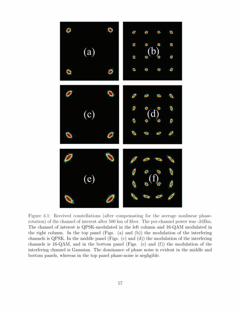
Figure 4.1: Received constellations (after compensating for the average nonlinear phase-rotation) of the channel of interest after 500 km of fiber. The per-channel power was -2dBm.The channel of interest is QPSK-modulated in the left column and 16-QAM modulated inthe right column. In the top panel (Figs. (a) and (b)) the modulation of the interferingchannels is QPSK. In the middle panel (Figs. (c) and (d)) the modulation of the interferingchannels is 16-QAM, and in the bottom panel (Figs. (e) and (f)) the modulation of theinterfering channel is Gaussian. The dominance of phase noise is evident in the middle andbottom panels, whereas in the top panel phase-noise is negligible.

57

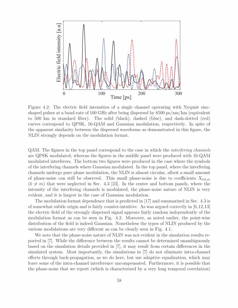
0 100 200 300Time [ps]

Ele

ctri

c fi

eld

in

ten

sity

[a.

u]

Figure 4.2: The electric field intensities of a single channel operating with Nyquist sinc-shaped pulses at a baud-rate of 100 GHz after being dispersed by 8500 ps/nm/km (equivalentto 500 km in standard fiber). The solid (black), dashed (blue), and dash-dotted (red)curves correspond to QPSK, 16-QAM and Gaussian modulation, respectively. In spite ofthe apparent similarity between the dispersed waveforms as demonstrated in this figure, theNLIN strongly depends on the modulation format.

QAM. The figures in the top panel correspond to the case in which the interfering channelsare QPSK modulated, whereas the figures in the middle panel were produced with 16-QAMmodulated interferers. The bottom two figures were produced in the case where the symbolsof the interfering channels where Gaussian modulated. In the top panel, where the interferingchannels undergo pure phase modulation, the NLIN is almost circular, albeit a small amountof phase-noise can still be observed. This small phase-noise is due to coefficients X0,k,m

(k 6= m) that were neglected in Sec. 4.3 [23]. In the center and bottom panels, where theintensity of the interfering channels is modulated, the phase-noise nature of NLIN is veryevident, and it is largest in the case of Gaussian modulation.

The modulation format dependence that is predicted in [17] and summarized in Sec. 4.3 isof somewhat subtle origin and is fairly counter-intuitive. As was argued correctly in [6,12,13]the electric field of the strongly dispersed signal appears fairly random independently of themodulation format as can be seen in Fig. 4.2. Moreover, as noted earlier, the point-wisedistribution of the field is indeed Gaussian. Nonetheless the types of NLIN produced by thevarious modulations are very different as can be clearly seen in Fig. 4.1.

We note that the phase-noise nature of NLIN was not evident in the simulation results re-ported in [7]. While the difference between the results cannot be determined unambiguouslybased on the simulation details provided in [7], it may result from certain differences in thesimulated system. Most importantly, the simulations in [7] do not eliminate intra-channeleffects through back-propagation, as we do here, but use adaptive equalization, which mayleave some of the intra-channel interference uncompensated. Furthermore, it is possible thatthe phase-noise that we report (which is characterized by a very long temporal correlation)

58

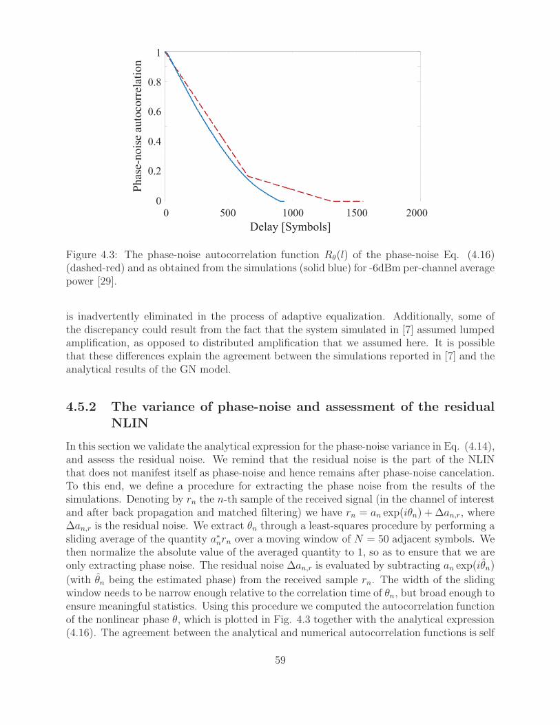
0 500 1000 1500 20000

0.2

0.4

0.6

0.8

1

Delay [Symbols]

Ph

ase-

no

ise

auto

corr

elat

ion

Figure 4.3: The phase-noise autocorrelation function Rθ(l) of the phase-noise Eq. (4.16)(dashed-red) and as obtained from the simulations (solid blue) for -6dBm per-channel averagepower [29].

is inadvertently eliminated in the process of adaptive equalization. Additionally, some ofthe discrepancy could result from the fact that the system simulated in [7] assumed lumpedamplification, as opposed to distributed amplification that we assumed here. It is possiblethat these differences explain the agreement between the simulations reported in [7] and theanalytical results of the GN model.

4.5.2 The variance of phase-noise and assessment of the residual

NLIN

In this section we validate the analytical expression for the phase-noise variance in Eq. (4.14),and assess the residual noise. We remind that the residual noise is the part of the NLINthat does not manifest itself as phase-noise and hence remains after phase-noise cancelation.To this end, we define a procedure for extracting the phase noise from the results of thesimulations. Denoting by rn the n-th sample of the received signal (in the channel of interestand after back propagation and matched filtering) we have rn = an exp(iθn) + ∆an,r, where∆an,r is the residual noise. We extract θn through a least-squares procedure by performing asliding average of the quantity a∗nrn over a moving window of N = 50 adjacent symbols. Wethen normalize the absolute value of the averaged quantity to 1, so as to ensure that we areonly extracting phase noise. The residual noise ∆an,r is evaluated by subtracting an exp(iθn)

(with θn being the estimated phase) from the received sample rn. The width of the slidingwindow needs to be narrow enough relative to the correlation time of θn, but broad enough toensure meaningful statistics. Using this procedure we computed the autocorrelation functionof the nonlinear phase θ, which is plotted in Fig. 4.3 together with the analytical expression(4.16). The agreement between the analytical and numerical autocorrelation functions is self

59

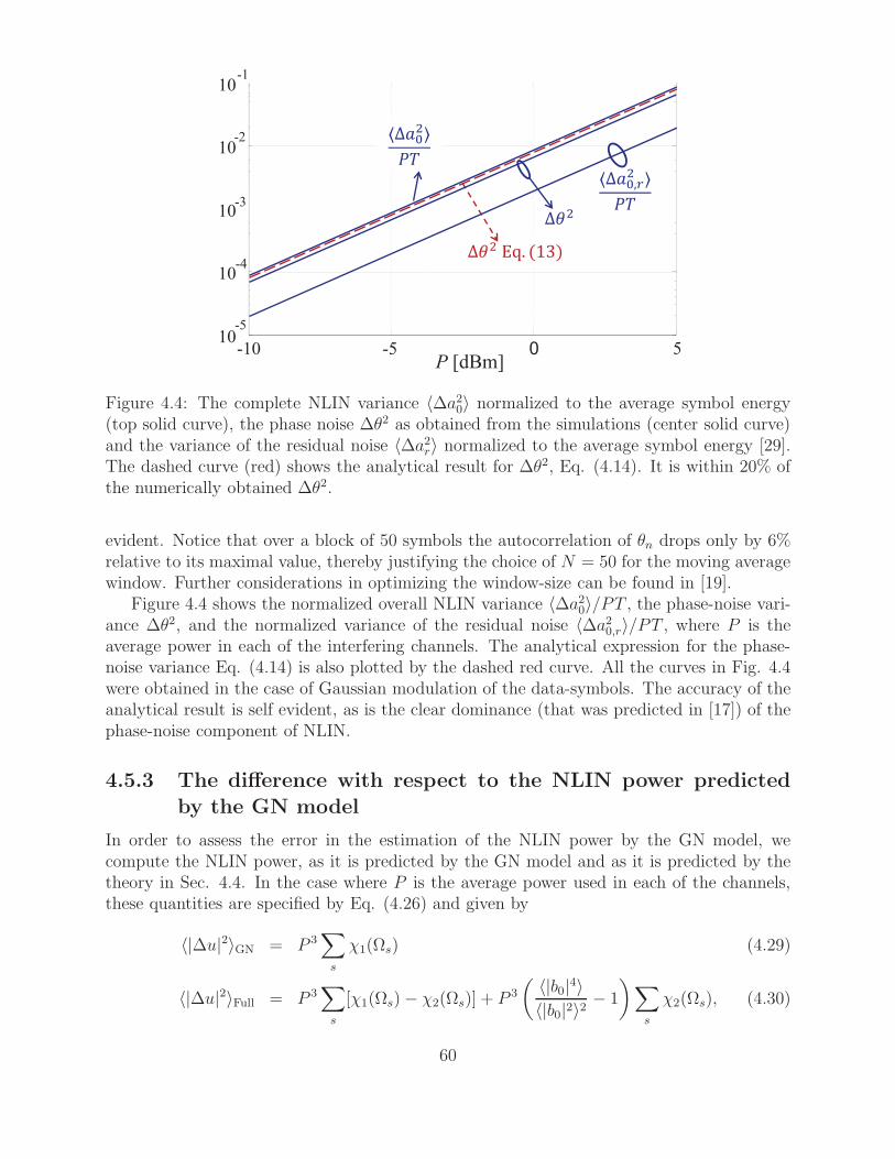
-10 -5 010

10

10

10

10

P [dBm]

-1

-2

-3

-4

-5

5

Figure 4.4: The complete NLIN variance 〈∆a20〉 normalized to the average symbol energy(top solid curve), the phase noise ∆θ2 as obtained from the simulations (center solid curve)and the variance of the residual noise 〈∆a2r〉 normalized to the average symbol energy [29].The dashed curve (red) shows the analytical result for ∆θ2, Eq. (4.14). It is within 20% ofthe numerically obtained ∆θ2.

evident. Notice that over a block of 50 symbols the autocorrelation of θn drops only by 6%relative to its maximal value, thereby justifying the choice of N = 50 for the moving averagewindow. Further considerations in optimizing the window-size can be found in [19].

Figure 4.4 shows the normalized overall NLIN variance 〈∆a20〉/PT , the phase-noise vari-ance ∆θ2, and the normalized variance of the residual noise 〈∆a20,r〉/PT , where P is theaverage power in each of the interfering channels. The analytical expression for the phase-noise variance Eq. (4.14) is also plotted by the dashed red curve. All the curves in Fig. 4.4were obtained in the case of Gaussian modulation of the data-symbols. The accuracy of theanalytical result is self evident, as is the clear dominance (that was predicted in [17]) of thephase-noise component of NLIN.

4.5.3 The difference with respect to the NLIN power predicted

by the GN model

In order to assess the error in the estimation of the NLIN power by the GN model, wecompute the NLIN power, as it is predicted by the GN model and as it is predicted by thetheory in Sec. 4.4. In the case where P is the average power used in each of the channels,these quantities are specified by Eq. (4.26) and given by

〈|∆u|2〉GN = P 3∑

s

χ1(Ωs) (4.29)

〈|∆u|2〉Full = P 3∑

s

[χ1(Ωs)− χ2(Ωs)] + P 3

( 〈|b0|4〉〈|b0|2〉2

− 1

)∑

s

χ2(Ωs), (4.30)

60

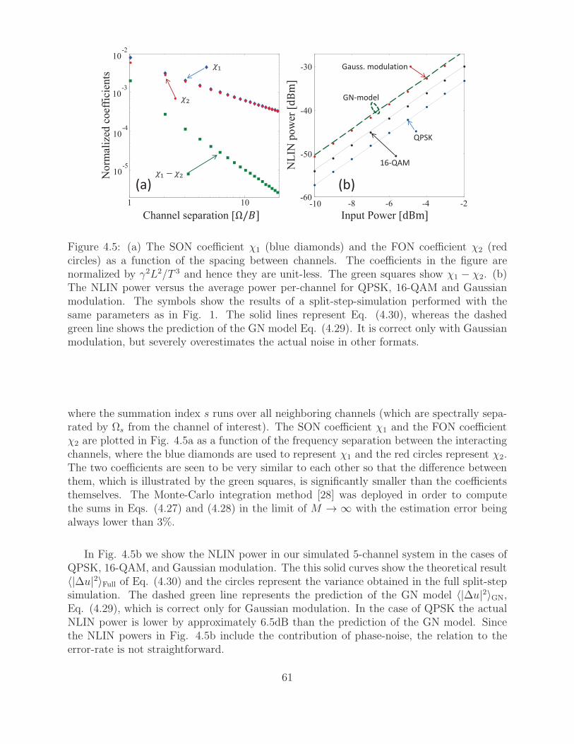
-10 -8 -6 -4 -2-60

-50

-40

-30

Channel separation [ Input Power [

NL

IN p

ow

er [

1 10

10 -2

10 -3

10 -4

10 -5

No

rmal

ized

co

effi

cien

ts

QPSK

16-QAM

GN-model

Gauss. modulation

(a) (b)

Figure 4.5: (a) The SON coefficient χ1 (blue diamonds) and the FON coefficient χ2 (redcircles) as a function of the spacing between channels. The coefficients in the figure arenormalized by γ2L2/T 3 and hence they are unit-less. The green squares show χ1 − χ2. (b)The NLIN power versus the average power per-channel for QPSK, 16-QAM and Gaussianmodulation. The symbols show the results of a split-step-simulation performed with thesame parameters as in Fig. 1. The solid lines represent Eq. (4.30), whereas the dashedgreen line shows the prediction of the GN model Eq. (4.29). It is correct only with Gaussianmodulation, but severely overestimates the actual noise in other formats.

where the summation index s runs over all neighboring channels (which are spectrally sepa-rated by Ωs from the channel of interest). The SON coefficient χ1 and the FON coefficientχ2 are plotted in Fig. 4.5a as a function of the frequency separation between the interactingchannels, where the blue diamonds are used to represent χ1 and the red circles represent χ2.The two coefficients are seen to be very similar to each other so that the difference betweenthem, which is illustrated by the green squares, is significantly smaller than the coefficientsthemselves. The Monte-Carlo integration method [28] was deployed in order to computethe sums in Eqs. (4.27) and (4.28) in the limit of M → ∞ with the estimation error beingalways lower than 3%.

In Fig. 4.5b we show the NLIN power in our simulated 5-channel system in the cases ofQPSK, 16-QAM, and Gaussian modulation. The this solid curves show the theoretical result〈|∆u|2〉Full of Eq. (4.30) and the circles represent the variance obtained in the full split-stepsimulation. The dashed green line represents the prediction of the GN model 〈|∆u|2〉GN,Eq. (4.29), which is correct only for Gaussian modulation. In the case of QPSK the actualNLIN power is lower by approximately 6.5dB than the prediction of the GN model. Sincethe NLIN powers in Fig. 4.5b include the contribution of phase-noise, the relation to theerror-rate is not straightforward.

61

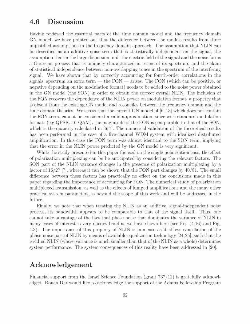
4.6 Discussion

Having reviewed the essential parts of the time domain model and the frequency domainGN model, we have pointed out that the difference between the models results from threeunjustified assumptions in the frequency domain approach. The assumption that NLIN canbe described as an additive noise term that is statistically independent on the signal, theassumption that in the large dispersion limit the electric field of the signal and the noise formsa Gaussian process that is uniquely characterized in terms of its spectrum, and the claimof statistical independence between non-overlapping tones in the spectrum of the interferingsignal. We have shown that by correctly accounting for fourth-order correlations in thesignals’ spectrum an extra term — the FON — arises. The FON (which can be positive, ornegative depending on the modulation format) needs to be added to the noise power obtainedin the GN model (the SON) in order to obtain the correct overall NLIN. The inclusion ofthe FON recovers the dependence of the NLIN power on modulation format, a property thatis absent from the existing GN model and reconciles between the frequency domain and thetime domain theories. We stress that the current GN model of [6–13] which does not containthe FON term, cannot be considered a valid approximation, since with standard modulationformats (e.g QPSK, 16-QAM), the magnitude of the FON is comparable to that of the SON,which is the quantity calculated in [6,7]. The numerical validation of the theoretical resultshas been performed in the case of a five-channel WDM system with idealized distributedamplification. In this case the FON term was almost identical to the SON term, implyingthat the error in the NLIN power predicted by the GN model is very significant.

While the study presented in this paper focused on the single polarization case, the effectof polarization multiplexing can be be anticipated by considering the relevant factors. TheSON part of the NLIN variance changes in the presence of polarization multiplexing by afactor of 16/27 [7], whereas it can be shown that the FON part changes by 40/81. The smalldifference between these factors has practically no effect on the conclusions made in thispaper regarding the importance of accounting for FON. The numerical study of polarizationmultiplexed transmission, as well as the effects of lumped amplifications and the many otherpractical system parameters, is beyond the scope of this work and will be addressed in thefuture.

Finally, we note that when treating the NLIN as an additive, signal-independent noiseprocess, its bandwidth appears to be comparable to that of the signal itself. Thus, onecannot take advantage of the fact that phase noise that dominates the variance of NLIN inmany cases of interest is very narrow-band as we have shown here (see Eq. (4.16) and Fig.4.3). The importance of this property of NLIN is immense as it allows cancelation of thephase-noise part of NLIN by means of available equalization technology [24,25], such that theresidual NLIN (whose variance is much smaller than that of the NLIN as a whole) determinessystem performance. The system consequences of this reality have been addressed in [20].

Acknowledgement

Financial support from the Israel Science Foundation (grant 737/12) is gratefully acknowl-edged. Ronen Dar would like to acknowledge the support of the Adams Fellowship Program

62

of the Israel Academy of Sciences and Humanities, and the Yitzhak and Chaya WeinsteinResearch Institute for Signal Processing. The authors acknowledge useful comments by P.JWinzer and A. Bononi.

63

Bibliography

[1] A. Mecozzi, C. B. Clausen, and M. Shtaif, “Analysis of intrachannel nonlinear effects inhighly dispersed optical pulse transmission,” IEEE Photon. Technol. Lett. 12, 392–394(2000).

[2] F. Forghieri, R.W. Tkack, A. R. Chraplyvy, “Fiber nonlinearities and their impact ontransmission systems,” Ch. 8 in Optical Fiber Telecommunications IIIA, P. Kaminowand T. L. Koch eds. Academic Press, 1997

[3] E. Ip, J.M. Kahn “Compensation of dispersion and nonlinear impairments using digitalbackpropagation,” J. Lightwave Technol. 26, 3416–3425 (2008).

[4] R. I. Killey, P. M. Watts, V. Mikhailov, M. Glick, P. Bayvel “Electronic dispersioncompensation by signal predistortion using digital processing and a dual-drive Mach-Zehnder modulator,” IEEE Photon. Technol. Lett., 17, 714–716 (2005).

[5] A. Splett, C. Kurtzke, K. Petermann, “Ultimate transmission capacity of amplifiedfiber communication systems taking into account fiber nonlinearities,” in 19th EuropeanConference on Optical Communication (ECOC), ECOC Technical Digest, (1993), PaperMoC2.4.

[6] P. Poggiolini, A. Carena, V. Curri, G. Bosco, and F. Forghieri, “Analytical modelingof nonlinear propagation in uncompensated optical transmission links,” IEEE Photon.Technol. Lett., 23, 742–744, (2011).

[7] A. Carena, V. Curri, G. Bosco, P. Poggiolini, and F. Forghieri, “Modeling of the Impactof Nonlinear Propagation Effects in Uncompensated Optical Coherent TransmissionLinks,” J. Lightwave Technol. 30, 1524–1539 (2012).

[8] P. Poggiolini, G. Bosco, A. Carena, V. Curri, and F. Forghieri, “A Detailed AnalyticalDerivation of the GN Model of Non-Linear Interference in Coherent Optical Transmis-sion Systems,” July 2, 2012 [Online]. Available: arXiv:1209.0394v12 [physics.optics].

[9] P. Poggiolini, “The GN Model of Non-Linear Propagation in Uncompensated CoherentOptical Systems,” J. of Lightwave Technol., 30, 3857–3879, (2012).

[10] A. Carena, G. Bosco, V. Curri, P. Poggiolini, M. Tapia Taiba, and F. Forghieri, “Sta-tistical characterization of PM-QPSK signals after propagation in uncompensated fiberlinks,” in Proc. ECOC, 2010, Paper P4.07.

64

[11] E. Torrengo, R. Cigliutti, G. Bosco, A. Carena, V. Curri, P. Poggiolini, A. Nespola, D.Zeolla, and F. Forghieri, “Experimental validation of an analytical model for nonlinearpropagation in uncompensated optical links,” in Proc. ECOC, 2011, Paper We.7.B.2.

[12] P. Johannisson and M. Karlsson, “Perturbation analysis of nonlinear propagation in astrongly dispersive optical communication system,” IEEE J. of Lightwave Technol., 31,1273–1282 (2013).

[13] A. Bononi, P. Serena “An alternative derivation of Johannissons regular perturbationmodel,” July 19, 2012 [Online]. Available: arXiv:1207.4729v1 [physics.optics].

[14] G. Bosco, R. Cigliutti, A. Nespola, A. Carena, V. Curri, F. Forghieri, Y. Yamamoto,T. Sasaki, Y. Jiang, P. Poggiolini, “Experimental investigation of nonlinear interferenceaccumulation in uncompensated links,” IEEE Photon. Technol. Lett. 24, 1230 – 1232,(2012)

[15] A. Bononi, N. Rossi, P. Serena, “Nonlinear Threshold Decrease with Distance in 112Gb/s PDM-QPSK Coherent Systems,” Proceeding of the European Conf. on Opt.Comm. (ECOC), Paper We.2.C.4, Amsterdam (2012)

[16] S.J. Savory, “Approximations for the Nonlinear Self-Channel Interference of ChannelsWith Rectangular Spectra,” IEEE Photon. Technol. Lett. 25, 961 – 964, (2013)

[17] A. Mecozzi and R. Essiambre, “Nonlinear Shannon Limit in Pseudolinear CoherentSystems,” J. Lightwave Technol. 30, 2011–2024 (2012).

[18] Xiang Liu, A. R. Chraplyvy, P. J. Winzer, R. W. Tkach, S. Chandrasekhar, “Phase-conjugated twin waves for communication beyond the Kerr nonlinearity limit,” NaturePhotonics 7, 560–568 (2013).

[19] Ronen Dar, Mark Shtaif, and Meir Feder, “New Bounds on the Capacity of Fiber-OpticsCommunications,” arXiv:1305.1762v1 [physics.optics].

[20] Ronen Dar, Mark Shtaif, and Meir Feder, “Improved Bounds on the Nonlinear Fiber-Channel Capacity,” in Proc. ECOC, 2013, paper P.4.16.

[21] S. Kumar and D. Yang, “Second-order theory for self-phase modulation andcross-phasemodulation in optical fibers,” J. of Lightwave Technol., 23, 2073 – 2080, (2005)

[22] We have assumed a fixed position independent dispersion parameter β ′′. The general-ization to position dependent dispersion is straightforward, but we avoid it as it consid-erably complicates the notation.

[23] Although terms involving X0,k,m with m 6= k also contribute to phase noise, they aremuch smaller than the terms proportional to X0,m,m (particularly in the limit of largedispersion) and we omit them from the analysis presented in this paper.

[24] X. Zhou, ”Hardware Efficient Carrier Recovery Algorithms for Single-Carrier QAMsystems,” in Advanced Photonics Congress, OSA Technical Digest (online) (OpticalSociety of America, 2012), paper SpTu3A.1.

65

[25] A. Tolmachev, I. Tselniker, M. Meltsin, I. Sigron, M. Nazarathy, “Efficient multiplier-free fpga demonstration of polar-domain multi-symbol-delay-detector (MSDD) for highperformance phase recovery of 16-QAM,” Proceedings of Optical Fiber Comm. Conf.OFC 2012, Paper OMC8

[26] A. Papoulis, “Pulse compression, fiber communications, and diffraction: a unified ap-proach,” J. Opt. Soc. Am. A 11, 3–13 (1994).

[27] R.-J. Essiambre, G. Kramer, P.J. Winzer, G.J. Foschini, and B. Goebel, “CapacityLimits of Optical Fiber Networks,” J. Lightwave Technol. 28, 662–701, (2010).

[28] S. Asmussen, P.W. Glynn, Stochastic simulation, algorithms and analysis, Springer,2007

[29] The numerical curves in Figs. 4.3 and 4.4 reproduce the plots reported in [20], but withlarger statsitics.

66

Chapter 5

New Bounds on the Capacity of the

Nonlinear Fiber-Optic ChannelRonen Dar, Mark Shtaif and Meir Feder, “New bounds on the capacity of the nonlinearfiber-optic channel,” Optics letters, vol. 39, pp. 398–401 (January 2014)

5.1 Abstract

We revisit the problem of estimating the nonlinear channel capacity of fiber-optic systems.By taking advantage of the fact that a large fraction of the nonlinear interference betweendifferent wavelength-division multiplexed channels manifests itself as phase noise, and byaccounting for the long temporal correlations of this noise, we show that the capacity is no-tably higher than what is currently assumed. This advantage is translated into the doublingof the link distance for a fixed transmission rate.

5.2 Introduction and results

Estimation of the fiber-optic channel capacity has come to be one of the most challenging andimportant problems in the field of optical communications [1–7]. Recently, its importancehas grown even higher as the latest capacity estimates are being rapidly approached by therates of commercial communications systems [8]. The difficulty in estimating the capacity ofthe fiber-optic channel is mostly due to the effect of fiber nonlinearity which generates com-plicated distortions of the transmitted optical waveforms. Perhaps the most comprehensiveand familiar attempt of estimating the fiber-channel capacity to date is due to Essiambreet al. [3], where it was argued that, under plausible assumptions on network architecture,nonlinear interference between different wavelength-division multiplexed (WDM) channelsmust be treated as noise, which was then identified as the predominant nonlinear factor inlimiting the capacity of the fiber-optic channel. This point of view has been adopted bymost subsequent studies [4–6], and we also adopt it in the study presented herein.

A common feature of capacity estimates published so far is that they treat the nonlinearnoise as additive, white and independent of the data transmitted on the channel of interest.In reality, in the presence of chromatic dispersion, different WDM channels propagate at

67

different velocities so that every symbol in the channel of interest interacts with multiplesymbols of every interfering channel. Consequently, adjacent symbols in the channel ofinterest are disturbed by essentially the same collection of interfering pulses and thereforethey are affected by nonlinearity in a highly correlated manner. In addition, as has beenrecently demonstrated in [6, 9], one of the most pronounced manifestations of nonlinearityis in the form of phase noise due to cross-phase modulation (XPM). The dominance of thephase noise nature of the nonlinear interference is particularly pronounced in systems withdistributed gain, which is the regime where the capacity of the fiber-optic channel has beenevaluated [3], and which is also assumed in the present work.

We demonstrate in what follows that by taking advantage of the long temporal correla-tions that allow the cancelation of nonlinear phase noise, it is possible to communicate ata higher rate than predicted in [3], or equivalently (almost) double the distance achievableat a given rate of communications. We stress that practical methods for canceling the non-linear phase noise are not discussed in this paper as we are only interested in the capacityimplications. We also note that nonlinear phase noise is canceled inadvertently in coherentoptical systems where an appropriately fast phase tracking algorithm is deployed.

We start by expressing the received signal samples after coherent detection and matchedfiltering as

yj = xj exp(iθj) + nNLj + nj , (5.1)

where j is the time index and the term nNLj accounts for all nonlinear noise contributions

that do not manifest themselves as phase noise. As in [3–6] we assume that the samples nNLj

are zero-mean statistically independent complex Gaussian variables with variance σ2NL. A

similar assumption holds for the amplified spontaneous emission (ASE) samples nj , whosevariance is denoted by σ2

ASE. All three noise contributions θj , nNLj , and nj are assumed to be

statistically independent of each other. All of the above assumptions, regarding the whitenessof nNL

j and nj, the statistical independence of all noise contributions and the Gaussianity ofnNLj constitute a worst case in terms of the resultant capacity [10, Ch. 10] and hence they

are in accord with our goal of deriving a capacity lower bound. Finally, consistently withwhat is suggested by the analysis in [6], we will also assume that θj is a Gaussian distributedvariable and its variance will be denoted by σ2

θ , whose expression can be found in [6, 9].For arriving at an analytical lower bound for the capacity, we assume that the nonlinear

phase noise θj is blockwise constant. In other words, it is assumed that the noise θj does notchange at all within a block of N symbols and then in the subsequent block it changes in astatistically independent manner. The assumption that θj does not change within a block isconsistent with the very long temporal correlations of the phase noise, as was demonstratedin [9, 11, 12]. The assumption of statistical independence of θj in adjacent blocks is again aworst-case scenario which is in accord with our interest in a lower bound.

The capacity of the block-wise independent phase noise channel (5.1) is given by

C =1

NsuppX

I(X ; Y ), (5.2)

where X and Y are column random vectors representing a block of N channel inputs andoutputs, respectively, in which the phase noise is constant. The term I(X; Y ) = h(Y ) −

68

h(Y |X) is the mutual information between the channel’s input and output, where h(·) isthe differential entropy. The supremum is over all input distributions satisfying the powerconstraint E[‖X‖2] = NP . In order to obtain a lower bound on the capacity we assignX a circular Gaussian distribution with statistically independent elements. Note that withthis input distribution, and taking into account the fact that nNL

j and nj are uncorrelatedwith the input signal [6,9], our assumption that these quantities are white circular Gaussianconstitutes a worst case scenario from the standpoint of the resultant capacity [10, Ch. 10,Ex. 1]. In this case Y is also a circularly symmetric complex Gaussian vector with differentialentropy h(Y ) = N log2(πe(P +σ2

eff)), where σ2eff is the variance of the effective additive noise,

i.e., σ2eff = σ2

ASE + σ2NL. The conditional distribution of Y given X is obviously not Gaussian

(see Eq. (5.1)), but since the Gaussian distribution maximizes the differential entropy of avector of zero-mean random variables with a given covariance matrix [10, Ch. 9, Theorem9.6.5], the differential entropy h(Y |X) satisfies

h(Y |X) = Ex

(h(Y |X = x)

)(5.3)

≤ 1

2Ex

(log2 det(2πe QY |X=x)

), (5.4)

where Y =[Re(Y )Im(Y )

]and QY |X=x is the covariance matrix of Y given X = x. By applying

some algebraic manipulations the determinant of QY |X=x can be shown to satisfy

det(QY |X=x) = (σ2eff

2)2N (1 + 2

‖x‖2σ2eff

σ2c )(1 + 2

‖x‖2σ2eff

σ2s ) , (5.5)

where the terms σ2c = 0.5(1 − e−σ2

θ )2 and σ2s = 0.5(1 − e−2σ2

θ ) are the variances of cos(θ)and sin(θ), respectively, and their calculation relies on the Gaussianity of θj . Note thatthroughout this paper the Gaussianity assumption of the phase noise is needed only here,for calculating σ2

c and σ2s . Finally, by plugging (5.5) into (5.4), the following capacity lower

bound is obtained

C ≥ log2

(1 +

P

σ2eff

)

− 1

2NEυ

log2

(1 + υσ2

c

P

σ2eff

)

− 1

2NEυ

log2

(1 + υσ2

s

P

σ2eff

), (5.6)

where the symbol Eυ stands for ensemble averaging with respect to a standard Chi-squaredistributed variable υ with 2N degrees of freedom. Notice that the first line on the right-hand-side of Eq. (5.6) follows from treating the nonlinear noise as white circular Gaussian– similarly to the analysis in [3]. Yet, the difference is that in our case σ2

NL corresponds onlyto the part of the nonlinear noise that does not manifest itself as phase noise and hence itis smaller than the nonlinear noise that is accounted for in [3]. The effect of phase noise onthe capacity is captured in our case by the bottom two lines on the right-hand-side of (5.6).This capacity loss, which may be viewed as a rate reduction needed for tracking the phasenoise, vanishes when the phase exhibits very long term correlations (i.e., when N → ∞).

69

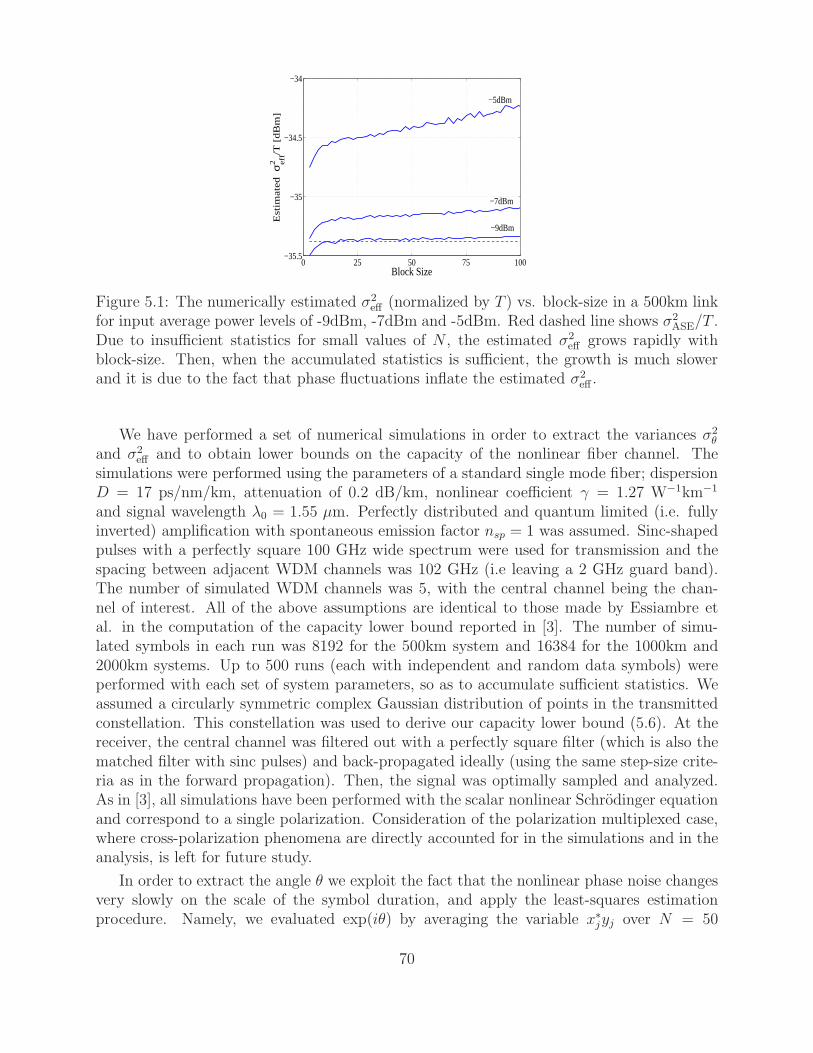
0 25 50 75 100−35.5

−35

−34.5

−34

Block SizeE

stim

ate

d σ

eff

2/T

[d

Bm

]

−9dBm

−7dBm

−5dBm

Figure 5.1: The numerically estimated σ2eff (normalized by T ) vs. block-size in a 500km link

for input average power levels of -9dBm, -7dBm and -5dBm. Red dashed line shows σ2ASE/T .

Due to insufficient statistics for small values of N , the estimated σ2eff grows rapidly with

block-size. Then, when the accumulated statistics is sufficient, the growth is much slowerand it is due to the fact that phase fluctuations inflate the estimated σ2

eff .

We have performed a set of numerical simulations in order to extract the variances σ2θ

and σ2eff and to obtain lower bounds on the capacity of the nonlinear fiber channel. The

simulations were performed using the parameters of a standard single mode fiber; dispersionD = 17 ps/nm/km, attenuation of 0.2 dB/km, nonlinear coefficient γ = 1.27 W−1km−1

and signal wavelength λ0 = 1.55 µm. Perfectly distributed and quantum limited (i.e. fullyinverted) amplification with spontaneous emission factor nsp = 1 was assumed. Sinc-shapedpulses with a perfectly square 100 GHz wide spectrum were used for transmission and thespacing between adjacent WDM channels was 102 GHz (i.e leaving a 2 GHz guard band).The number of simulated WDM channels was 5, with the central channel being the chan-nel of interest. All of the above assumptions are identical to those made by Essiambre etal. in the computation of the capacity lower bound reported in [3]. The number of simu-lated symbols in each run was 8192 for the 500km system and 16384 for the 1000km and2000km systems. Up to 500 runs (each with independent and random data symbols) wereperformed with each set of system parameters, so as to accumulate sufficient statistics. Weassumed a circularly symmetric complex Gaussian distribution of points in the transmittedconstellation. This constellation was used to derive our capacity lower bound (5.6). At thereceiver, the central channel was filtered out with a perfectly square filter (which is also thematched filter with sinc pulses) and back-propagated ideally (using the same step-size crite-ria as in the forward propagation). Then, the signal was optimally sampled and analyzed.As in [3], all simulations have been performed with the scalar nonlinear Schrodinger equationand correspond to a single polarization. Consideration of the polarization multiplexed case,where cross-polarization phenomena are directly accounted for in the simulations and in theanalysis, is left for future study.

In order to extract the angle θ we exploit the fact that the nonlinear phase noise changesvery slowly on the scale of the symbol duration, and apply the least-squares estimationprocedure. Namely, we evaluated exp(iθ) by averaging the variable x∗jyj over N = 50

70

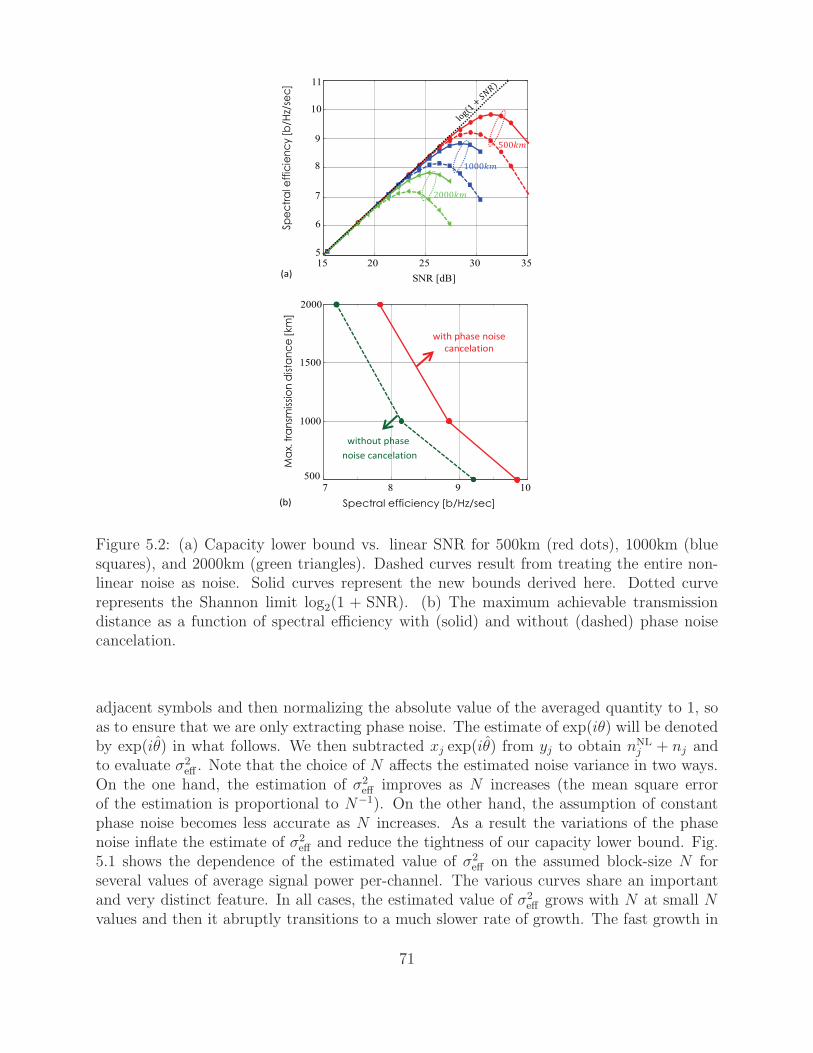
11

10

9

8

7

6

515 20 25 30 35

]Sp

ec

tra

l eff

icie

nc

y [

b/H

z/se

cSNR [dB]

(a)

(b)

7 8 9 10

500

1000

1500

2000

]Spectral efficiency [b/Hz/sec

Ma

x.tr

an

smis

sio

n d

ista

nc

e [

km

]

without phase

noise cancelation

with phase noise

cancelation

500

1000

2000

Figure 5.2: (a) Capacity lower bound vs. linear SNR for 500km (red dots), 1000km (bluesquares), and 2000km (green triangles). Dashed curves result from treating the entire non-linear noise as noise. Solid curves represent the new bounds derived here. Dotted curverepresents the Shannon limit log2(1 + SNR). (b) The maximum achievable transmissiondistance as a function of spectral efficiency with (solid) and without (dashed) phase noisecancelation.

adjacent symbols and then normalizing the absolute value of the averaged quantity to 1, soas to ensure that we are only extracting phase noise. The estimate of exp(iθ) will be denotedby exp(iθ) in what follows. We then subtracted xj exp(iθ) from yj to obtain nNL

j + nj andto evaluate σ2

eff . Note that the choice of N affects the estimated noise variance in two ways.On the one hand, the estimation of σ2

eff improves as N increases (the mean square errorof the estimation is proportional to N−1). On the other hand, the assumption of constantphase noise becomes less accurate as N increases. As a result the variations of the phasenoise inflate the estimate of σ2

eff and reduce the tightness of our capacity lower bound. Fig.5.1 shows the dependence of the estimated value of σ2

eff on the assumed block-size N forseveral values of average signal power per-channel. The various curves share an importantand very distinct feature. In all cases, the estimated value of σ2

eff grows with N at small Nvalues and then it abruptly transitions to a much slower rate of growth. The fast growth in

71

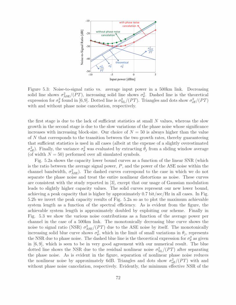
10-

20-

30-

40-

50-10- 5- 50

Input power [dBm]N

ois

e-to

-Sig

nal

Rat

io [

dB

]

theoretical

with phase noise

cancelation

without phase noise

cancelation

Figure 5.3: Noise-to-signal ratio vs. average input power in a 500km link. Decreasingsolid line shows σ2

ASE/(PT ), increasing solid line shows σ2θ . Dashed line is the theoretical

expression for σ2θ found in [6,9]. Dotted line is σ2

NL/(PT ). Triangles and dots show σ2eff/(PT )

with and without phase noise cancelation, respectively.

the first stage is due to the lack of sufficient statistics at small N values, whereas the slowgrowth in the second stage is due to the slow variations of the phase noise whose significanceincreases with increasing block-size. Our choice of N = 50 is always higher than the valueof N that corresponds to the transition between the two growth rates, thereby guaranteeingthat sufficient statistics is used in all cases (albeit at the expense of a slightly overestimatedσ2eff). Finally, the variance σ2

θ was evaluated by extracting θj from a sliding window average(of width N = 50) performed over all simulated symbols.

Fig. 5.2a shows the capacity lower bound curves as a function of the linear SNR (whichis the ratio between the average signal power, P , and the power of the ASE noise within thechannel bandwidth, σ2

ASE). The dashed curves correspond to the case in which we do notseparate the phase noise and treat the entire nonlinear distortions as noise. These curvesare consistent with the study reported in [3], except that our usage of Gaussian modulationleads to slightly higher capacity values. The solid curves represent our new lower bound,achieving a peak capacity that is higher by approximately 0.7 bit/sec/Hz in all cases. In Fig.5.2b we invert the peak capacity results of Fig. 5.2a so as to plot the maximum achievablesystem length as a function of the spectral efficiency. As is evident from the figure, theachievable system length is approximately doubled by exploiting our scheme. Finally inFig. 5.3 we show the various noise contributions as a function of the average power perchannel in the case of a 500km link. The monotonically decreasing blue curve shows thenoise to signal ratio (NSR) σ2

ASE/(PT ) due to the ASE noise by itself. The monotonicallyincreasing solid blue curve shows σ2

θ , which in the limit of small variations in θj , representsthe NSR due to phase noise. The dashed blue line is the theoretical expression for σ2

θ as givenin [6, 9], which is seen to be in very good agreement with our numerical result. The bluedotted line shows the NSR due to the residual nonlinear noise σ2

NL/(PT ) after separatingthe phase noise. As is evident in the figure, separation of nonlinear phase noise reducesthe nonlinear noise by approximately 6dB. Triangles and dots show σ2

eff/(PT ) with andwithout phase noise cancelation, respectively. Evidently, the minimum effective NSR of the

72

system is improved by approximately 2dB. We note that to facilitate the distinction betweenthe noise contributions the simulation that produced Fig. 5.3 was performed without ASEpropagation. In Figs. 5.2a and 5.2b ASE noise was propagated, although similar resultswere observed when the ASE was added at the end. We also note that these figures wereobtained using more statistics than those presented in [11].

5.3 Conclusions

We have derived a new lower bound for the capacity of the nonlinear fiber channel by takinginto account the fact that phase noise is one of the the most significant consequences ofnonlinear interference, and by taking advantage of the fact that this noise is characterizedby strong temporal correlations. We showed that the peak capacity per polarization canbe increased by approximately 0.7bit/s/Hz or equivalently the length of a system can be(almost) doubled for a given transmission rate.

Acknowledgement

The authors would like to acknowledge financial support from the Israel Science Foundation(grant 737/12). Ronen Dar would like to acknowledge the support of the Adams FellowshipProgram of the Israel Academy of Sciences and Humanities, and the Yitzhak and ChayaWeinstein Research Institute for Signal Processing. Fruitful discussions with R. J. Essiambreare also gratefully acknowledged.

73

Bibliography

[1] P. P. Mitra and J. B. Stark, “Nonlinear limits to the information capacity of opticalfibre communications,”Nature 411, 1027–1030 (2001).

[2] K. S. Turitsyn, S. A. Derevyanko, I. V. Yurkevich, and S. K. Turitsyn, “Informationcapacity of optical fiber channels with zero average dispersion,”Physical review letters91, 203901–203904 (2003).

[3] R.-J. Essiambre, G. Kramer, P. J. Winzer, G. J. Foschini, and B. Goebel, “Capacitylimits of optical fiber networks,”J. Lightwave Technol. 28, 662–701 (2010).

[4] A. D. Ellis, J. Zhao, and D. Cotter, “Approaching the non-linear Shannon limit,”J.Lightwave Technol. 28, 423–433 (2010).

[5] G. Bosco, P. Poggiolini, A. Carena, V. Curri, and F. Forghieri, “Analytical resultson channel capacity in uncompensated optical links with coherent detection,”Opt. Ex-press19, B440–B451 (2011).

[6] A. Mecozzi and R.-J. Essiambre, “Nonlinear Shannon limit in pseudolinear coherentsystems,”J. Lightwave Technol. 30, 2011–2024 (2012).

[7] E. Agrell and M. Karlsson, “WDM channel capacity and its dependence on multichanneladaptation models,”Optical Fiber Communication Conference 2013 (OFC13).

[8] P. J. Winzer and G. J. Foschini, “MIMO capacities and outage probabilities in spatiallymultiplexed optical transport systems,”Opt. Express19, 16680–96 (2011).

[9] R. Dar, M. Feder, A. Mecozzi, and M. Shtaif, “Properties of nonlinear noise in long,dispersion-uncompensated fiber links,”Opt. Express21, 25685–25699 (2013).

[10] T. M. Cover and J. A. Thomas, “Elements of information theory,”(Wiley, 1991).

[11] R. Dar, M. Shtaif, and M. Feder, “Improved bounds on the nonlinear fiber-channel ca-pacity,”European Conference on Optical Communication 2013 (ECOC13), paper P.4.16(2013).

[12] With system parameters similar to those used for evaluating the capacity in [3] andassuming for example a 500km link, the phase has been shown to be nearly constant onthe scale of a few tens of symbol durations [9].

74

[13] A. Lapidoth and S. M. Moser, “Capacity bounds via duality with applications tomultiple-antenna systems on flat-fading channels,”IEEE Trans. on IT 49, 25685–25699(2003).

75

Chapter 6

Accumulation of Nonlinear

Interference Noise in Fiber-Optic

SystemsRonen Dar, Meir Feder, Antonio Mecozzi and Mark Shtaif, “Accumulation of nonlinearinterference noise in fiber-optic systems,” Optics express, vol. 22, pp. 14199–14211 (June2014)

6.1 Abstract

Through a series of extensive system simulations we show that all of the previously notunderstood discrepancies between the Gaussian noise (GN) model and simulations can beattributed to the omission of an important, recently reported, fourth-order noise (FON)term, that accounts for the statistical dependencies within the spectrum of the interferingchannel. We examine the importance of the FON term as well as the dependence of NLINon modulation format with respect to link-length and number of spans. A computationallyefficient method for evaluating the FON contribution, as well as the overall NLIN power isprovided.

6.2 Introduction

Inter-channel nonlinear interference is arguably the most important factor in limiting theperformance of fiber-optic communications [1]. Since joint processing of the entire WDMspectrum of channels is prohibitively complex, nonlinear interference between channels iscustomarily treated as noise. The statistical characterization of this noise — to which werefer in what follows as nonlinear interference noise (NLIN) — is the goal of most recenttheoretical studies of nonlinear transmission [2–9]. Understanding the features of NLIN iscritical for the efficient design of fiber-optic systems and for the accurate prediction of theirperformance.

Most of the available work on NLIN in fiber-optic systems was published in the contextof the Gaussian noise (GN) model [2–5], which describes NLIN as an additive Gaussian

77

noise process whose variance and spectrum it evaluates. The validation of the GN modeland the characterization of its accuracy have been the subject of numerous studies (e.g.see [3, 4]). It was found that while the model’s accuracy is satisfactory in some scenarios, itis highly inadequate in others. Some of the GN model’s most conspicuous shortcomings areits independence of modulation format [6], its independence of pre-dispersion [4], and its largeinaccuracy in predicting the growth of the NLIN variance with the number of spans in anamplified multi-span link [3,4]. Although phenomenological fixes for the latter problem havebeen proposed (most notably through the practice of accumulating the NLIN contributionsof various spans incoherently [2–4]), the remedy that they offered remained limited, and thefundamental reason for the observed behavior has never been understood.

We argue, similarly to [6], that the reason for the inaccuracy of the GN approach is inignoring the statistical dependence between different frequency components of the interferingchannel. Accounting for this dependence produces an important correction term to which werefer (for reasons explained in the following section) as the fourth-order noise or FON. Bysimulating a number of fiber-systems in the relevant range of parameters, we demonstratethat the FON term resolves all of the reported inaccuracies of the GN model, including thedependence on modulation format, signal pre-dispersion, and the accumulation of NLIN withthe number of spans.

We stress that as demonstrated in [6] the NLIN is not an additive Gaussian process, andhence its variance (and even its entire spectrum) does not characterize its properties in asatisfactory manner. For example, as pointed out in [8], part of the NLIN manifests itselfas phase-noise, whose effect in terms of transmission performance is very different from thatof additive noise [10]. We show in what follows that the phase-noise character of NLIN,as well as the dependence of NLIN on modulation format is largest in the case of a singleamplified span, or in a system of arbitrary length that uses distributed amplification (asin [6]). The distinctness of these properties reduces somewhat in multi-span systems withlumped amplification and with a span-length much larger than the fiber’s effective length.

In order to facilitate future research of this problem, we provide a computer programthat implements a computationally efficient algorithm for computing the SON and the FONcoefficients that are needed for reproducing the theoretical curves that we present in thispaper. For the reader’s convenience, the program also includes the option of computing theentire NLIN variance, including intra-channel interference terms, as well as inter-channelinterference terms that are not directly addressed in the main text of this paper, and whichhave been recently posted in [7]. The contribution of these terms reduces very rapidlywith channel spacing and while one may generate situations in which inclusion of theseterms becomes relevant, they were negligible in the system studied in [6] (which assumeddistributed amplification, and a guard-band as small as 2%), and they are also negligible insystems with more realistic parameters, as considered here. We note that while the full scalesimulations of the systems of interest are computationally intense and time consuming, theextraction of NLIN power on the basis of the FON and SON coefficients that we provide ispractically instantaneous.

78

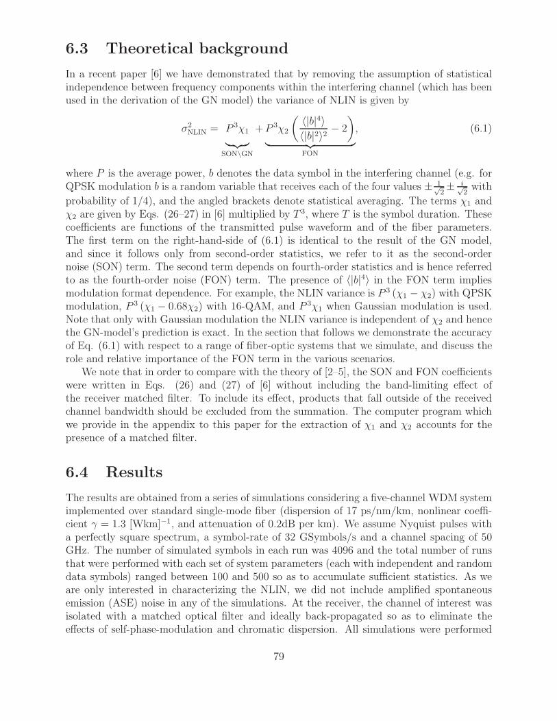
6.3 Theoretical background

In a recent paper [6] we have demonstrated that by removing the assumption of statisticalindependence between frequency components within the interfering channel (which has beenused in the derivation of the GN model) the variance of NLIN is given by

σ2NLIN = P 3χ1

︸︷︷︸SON\GN

+P 3χ2

( 〈|b|4〉〈|b|2〉2 − 2

)

︸︷︷︸FON

, (6.1)

where P is the average power, b denotes the data symbol in the interfering channel (e.g. forQPSK modulation b is a random variable that receives each of the four values ± 1√

2± i√

2with

probability of 1/4), and the angled brackets denote statistical averaging. The terms χ1 andχ2 are given by Eqs. (26–27) in [6] multiplied by T 3, where T is the symbol duration. Thesecoefficients are functions of the transmitted pulse waveform and of the fiber parameters.The first term on the right-hand-side of (6.1) is identical to the result of the GN model,and since it follows only from second-order statistics, we refer to it as the second-ordernoise (SON) term. The second term depends on fourth-order statistics and is hence referredto as the fourth-order noise (FON) term. The presence of 〈|b|4〉 in the FON term impliesmodulation format dependence. For example, the NLIN variance is P 3 (χ1 − χ2) with QPSKmodulation, P 3 (χ1 − 0.68χ2) with 16-QAM, and P 3χ1 when Gaussian modulation is used.Note that only with Gaussian modulation the NLIN variance is independent of χ2 and hencethe GN-model’s prediction is exact. In the section that follows we demonstrate the accuracyof Eq. (6.1) with respect to a range of fiber-optic systems that we simulate, and discuss therole and relative importance of the FON term in the various scenarios.

We note that in order to compare with the theory of [2–5], the SON and FON coefficientswere written in Eqs. (26) and (27) of [6] without including the band-limiting effect ofthe receiver matched filter. To include its effect, products that fall outside of the receivedchannel bandwidth should be excluded from the summation. The computer program whichwe provide in the appendix to this paper for the extraction of χ1 and χ2 accounts for thepresence of a matched filter.

6.4 Results

The results are obtained from a series of simulations considering a five-channel WDM systemimplemented over standard single-mode fiber (dispersion of 17 ps/nm/km, nonlinear coeffi-cient γ = 1.3 [Wkm]−1, and attenuation of 0.2dB per km). We assume Nyquist pulses witha perfectly square spectrum, a symbol-rate of 32 GSymbols/s and a channel spacing of 50GHz. The number of simulated symbols in each run was 4096 and the total number of runsthat were performed with each set of system parameters (each with independent and randomdata symbols) ranged between 100 and 500 so as to accumulate sufficient statistics. As weare only interested in characterizing the NLIN, we did not include amplified spontaneousemission (ASE) noise in any of the simulations. At the receiver, the channel of interest wasisolated with a matched optical filter and ideally back-propagated so as to eliminate theeffects of self-phase-modulation and chromatic dispersion. All simulations were performed

79

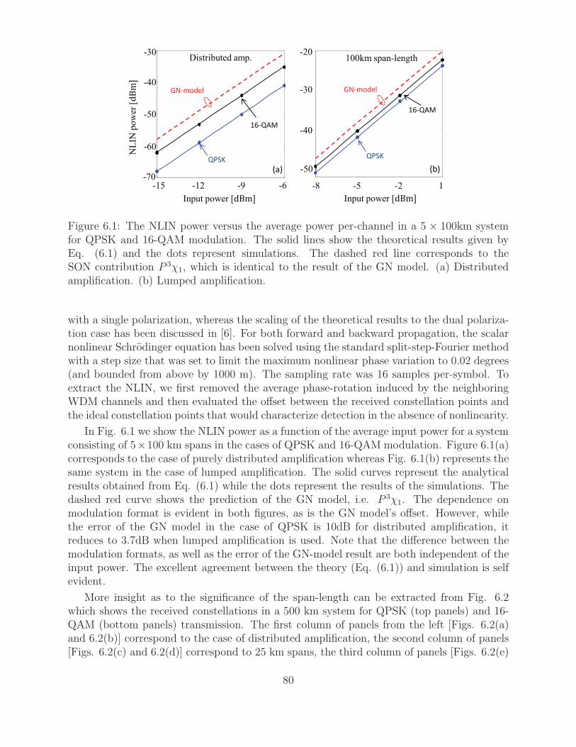
100km span-length

GN-model

8- 5- 2- 1

40-

30-

20-

Input power [dBm]

(b)50-

GN-model

Distributed amp.

-15 -12 -9 -6

-60

-50

-40

-30

NL

IN p

ow

er [dBm]

(a)

Input power [dBm]

-70

QPSK

16-QAM

QPSK

16-QAM

Figure 6.1: The NLIN power versus the average power per-channel in a 5 × 100km systemfor QPSK and 16-QAM modulation. The solid lines show the theoretical results given byEq. (6.1) and the dots represent simulations. The dashed red line corresponds to theSON contribution P 3χ1, which is identical to the result of the GN model. (a) Distributedamplification. (b) Lumped amplification.

with a single polarization, whereas the scaling of the theoretical results to the dual polariza-tion case has been discussed in [6]. For both forward and backward propagation, the scalarnonlinear Schrodinger equation has been solved using the standard split-step-Fourier methodwith a step size that was set to limit the maximum nonlinear phase variation to 0.02 degrees(and bounded from above by 1000 m). The sampling rate was 16 samples per-symbol. Toextract the NLIN, we first removed the average phase-rotation induced by the neighboringWDM channels and then evaluated the offset between the received constellation points andthe ideal constellation points that would characterize detection in the absence of nonlinearity.

In Fig. 6.1 we show the NLIN power as a function of the average input power for a systemconsisting of 5×100 km spans in the cases of QPSK and 16-QAM modulation. Figure 6.1(a)corresponds to the case of purely distributed amplification whereas Fig. 6.1(b) represents thesame system in the case of lumped amplification. The solid curves represent the analyticalresults obtained from Eq. (6.1) while the dots represent the results of the simulations. Thedashed red curve shows the prediction of the GN model, i.e. P 3χ1. The dependence onmodulation format is evident in both figures, as is the GN model’s offset. However, whilethe error of the GN model in the case of QPSK is 10dB for distributed amplification, itreduces to 3.7dB when lumped amplification is used. Note that the difference between themodulation formats, as well as the error of the GN-model result are both independent of theinput power. The excellent agreement between the theory (Eq. (6.1)) and simulation is selfevident.

More insight as to the significance of the span-length can be extracted from Fig. 6.2which shows the received constellations in a 500 km system for QPSK (top panels) and 16-QAM (bottom panels) transmission. The first column of panels from the left [Figs. 6.2(a)and 6.2(b)] correspond to the case of distributed amplification, the second column of panels[Figs. 6.2(c) and 6.2(d)] correspond to 25 km spans, the third column of panels [Figs. 6.2(e)

80

500km

distributed amp. 20 x 25km 10 x 50km 5 x 100km

16

-QA

MQ

PS

K

(g)

(c)

(d)

(e)

(f)

(g)

(h)

(c)

(d)(b)

(a)

Figure 6.2: Constellation diagrams for QPSK (top panels) and 16-QAM (bottom panels) inthe cases of distributed amplification (a and b), 25 km spans (c and d), 50 km (e and f) and100 km (g and h). In all cases a path-averaged power of -10dBm was used. The phase noisenature of NLIN is evident in the case of 16-QAM modulation, but its relative significancereduces when the span-length is large. The 100 km span case is closer to the circular noisedistributions observed in [3].

and 6.2(f)] correspond to 50 km spans and the case of 100 km spans is shown in the rightmostpanels [Figs. 6.2(g) and 6.2(h)]. Here and in the figures that follow, the launched powers wereselected such that the path-averaged power per-channel was -10dBm in all cases (input powerof -7.7dBm, -5.9dBm and -3.3dBm, for 25 km, 50 km, and 100 km spans, respectively). Useof a constant path-averaged power is customary when comparing systems with different spanlengths [11], and the value of -10dBm was found to be roughly optimal from the standpointof capacity maximization in the distributed amplification case [8]. As can be seen in Fig.6.1, the comparison between modulation formats is practically independent of the launchedoptical power. Consistently with the predictions in [6], the phase noise is negligible in the caseof QPSK transmission, and the constellation points are nearly circular for all span-lengths.With 16-QAM modulation, phase-noise is dominant in the case of distributed amplificationand 25 km spans, whereas at longer span-lengths the phase-noise character of NLIN becomesless evident. We note that even in the case of 100 km spans, phase noise is clearly visibleimplying that NLIN cannot be accurately described as additive, although the error fromdoing so is notably smaller.

Figure 6.3 shows the accumulation of NLIN along systems of different span-lengths.Fig. 6.3(a) shows the case of distributed amplification whereas Figs. 6.3(b)-6.3(d) show

81

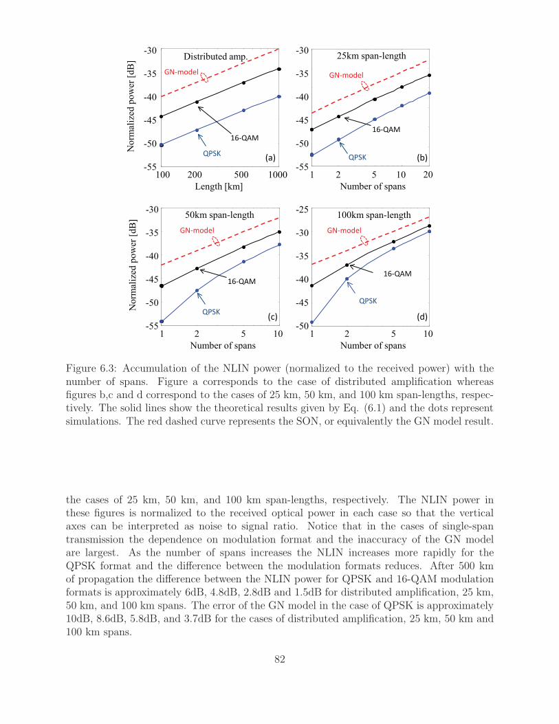
QPSK

16-QAM

GN-model

(d)

100km span-length

10

45-

40-

35-

30-

-25

Number of spans

52150-

QPSK

16-QAM

GN-model

(b)

10

50-

45-

40-

35-

-30

52155-

20

25km span-length

QPSK

16-QAM

50km span-length

GN-model

(c)

10

50-

45-

40-

35-

-30

Number of spans

52155-

No

rmal

ized

po

wer

[d

B]

Number of spans

QPSK

16-QAM

Distributed amp.

GN-model

(a)

1000

50-

45-

40-

35-

-30

Length [km]

50020010055-

No

rmal

ized

po

wer

[d

B]

Figure 6.3: Accumulation of the NLIN power (normalized to the received power) with thenumber of spans. Figure a corresponds to the case of distributed amplification whereasfigures b,c and d correspond to the cases of 25 km, 50 km, and 100 km span-lengths, respec-tively. The solid lines show the theoretical results given by Eq. (6.1) and the dots representsimulations. The red dashed curve represents the SON, or equivalently the GN model result.

the cases of 25 km, 50 km, and 100 km span-lengths, respectively. The NLIN power inthese figures is normalized to the received optical power in each case so that the verticalaxes can be interpreted as noise to signal ratio. Notice that in the cases of single-spantransmission the dependence on modulation format and the inaccuracy of the GN modelare largest. As the number of spans increases the NLIN increases more rapidly for theQPSK format and the difference between the modulation formats reduces. After 500 kmof propagation the difference between the NLIN power for QPSK and 16-QAM modulationformats is approximately 6dB, 4.8dB, 2.8dB and 1.5dB for distributed amplification, 25 km,50 km, and 100 km spans. The error of the GN model in the case of QPSK is approximately10dB, 8.6dB, 5.8dB, and 3.7dB for the cases of distributed amplification, 25 km, 50 km and100 km spans.

82

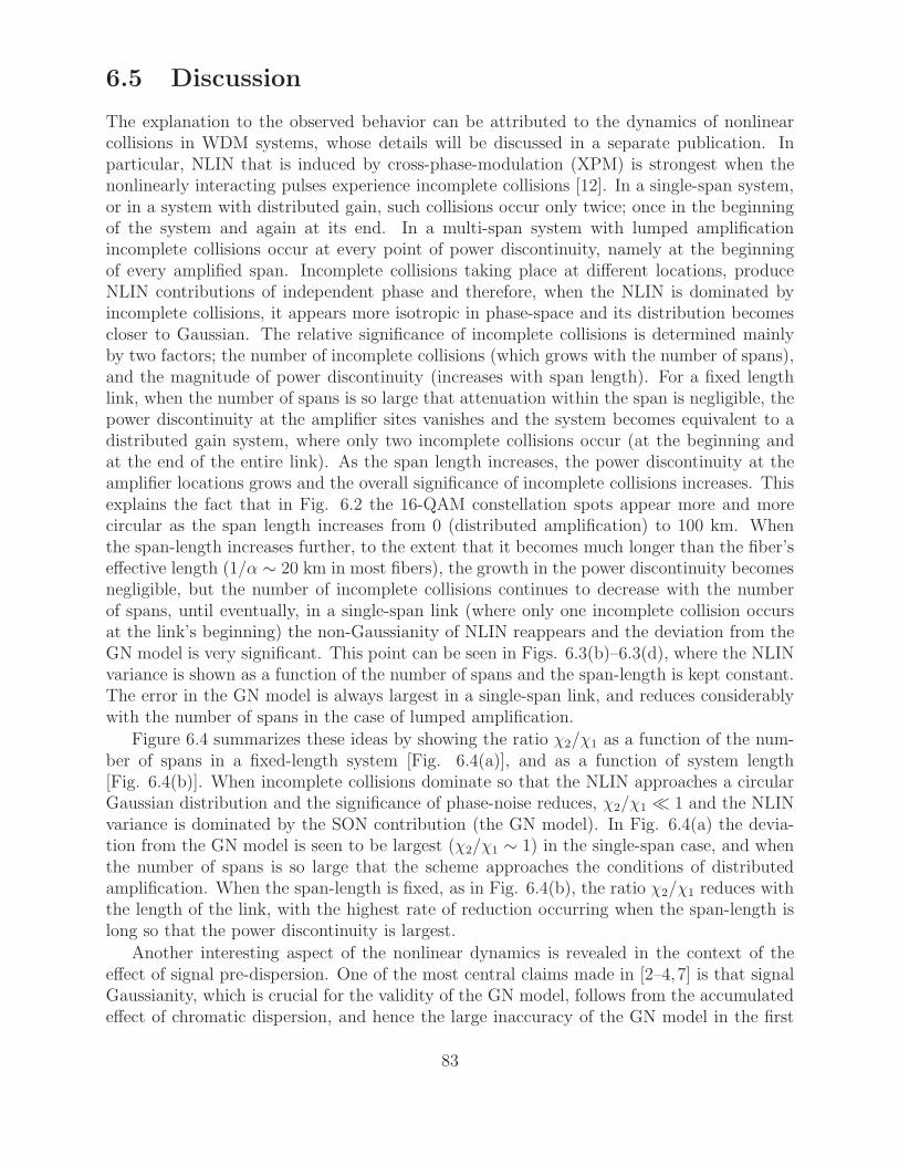
6.5 Discussion

The explanation to the observed behavior can be attributed to the dynamics of nonlinearcollisions in WDM systems, whose details will be discussed in a separate publication. Inparticular, NLIN that is induced by cross-phase-modulation (XPM) is strongest when thenonlinearly interacting pulses experience incomplete collisions [12]. In a single-span system,or in a system with distributed gain, such collisions occur only twice; once in the beginningof the system and again at its end. In a multi-span system with lumped amplificationincomplete collisions occur at every point of power discontinuity, namely at the beginningof every amplified span. Incomplete collisions taking place at different locations, produceNLIN contributions of independent phase and therefore, when the NLIN is dominated byincomplete collisions, it appears more isotropic in phase-space and its distribution becomescloser to Gaussian. The relative significance of incomplete collisions is determined mainlyby two factors; the number of incomplete collisions (which grows with the number of spans),and the magnitude of power discontinuity (increases with span length). For a fixed lengthlink, when the number of spans is so large that attenuation within the span is negligible, thepower discontinuity at the amplifier sites vanishes and the system becomes equivalent to adistributed gain system, where only two incomplete collisions occur (at the beginning andat the end of the entire link). As the span length increases, the power discontinuity at theamplifier locations grows and the overall significance of incomplete collisions increases. Thisexplains the fact that in Fig. 6.2 the 16-QAM constellation spots appear more and morecircular as the span length increases from 0 (distributed amplification) to 100 km. Whenthe span-length increases further, to the extent that it becomes much longer than the fiber’seffective length (1/α ∼ 20 km in most fibers), the growth in the power discontinuity becomesnegligible, but the number of incomplete collisions continues to decrease with the numberof spans, until eventually, in a single-span link (where only one incomplete collision occursat the link’s beginning) the non-Gaussianity of NLIN reappears and the deviation from theGN model is very significant. This point can be seen in Figs. 6.3(b)–6.3(d), where the NLINvariance is shown as a function of the number of spans and the span-length is kept constant.The error in the GN model is always largest in a single-span link, and reduces considerablywith the number of spans in the case of lumped amplification.

Figure 6.4 summarizes these ideas by showing the ratio χ2/χ1 as a function of the num-ber of spans in a fixed-length system [Fig. 6.4(a)], and as a function of system length[Fig. 6.4(b)]. When incomplete collisions dominate so that the NLIN approaches a circularGaussian distribution and the significance of phase-noise reduces, χ2/χ1 ≪ 1 and the NLINvariance is dominated by the SON contribution (the GN model). In Fig. 6.4(a) the devia-tion from the GN model is seen to be largest (χ2/χ1 ∼ 1) in the single-span case, and whenthe number of spans is so large that the scheme approaches the conditions of distributedamplification. When the span-length is fixed, as in Fig. 6.4(b), the ratio χ2/χ1 reduces withthe length of the link, with the highest rate of reduction occurring when the span-length islong so that the power discontinuity is largest.

Another interesting aspect of the nonlinear dynamics is revealed in the context of theeffect of signal pre-dispersion. One of the most central claims made in [2–4,7] is that signalGaussianity, which is crucial for the validity of the GN model, follows from the accumulatedeffect of chromatic dispersion, and hence the large inaccuracy of the GN model in the first

83

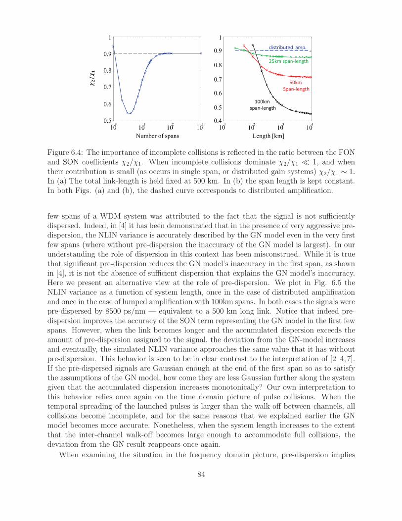
100

0.5

/

0.6

0.7

0.8

0.9

1

101

102

103

Number of spans

101

0.5

0.6

0.7

0.8

0.9

1

102

103

104

Length [km]

0.4

50km

Span-length

25km span-length

100km

span-length

distributed amp.

Figure 6.4: The importance of incomplete collisions is reflected in the ratio between the FONand SON coefficients χ2/χ1. When incomplete collisions dominate χ2/χ1 ≪ 1, and whentheir contribution is small (as occurs in single span, or distributed gain systems) χ2/χ1 ∼ 1.In (a) The total link-length is held fixed at 500 km. In (b) the span length is kept constant.In both Figs. (a) and (b), the dashed curve corresponds to distributed amplification.

few spans of a WDM system was attributed to the fact that the signal is not sufficientlydispersed. Indeed, in [4] it has been demonstrated that in the presence of very aggressive pre-dispersion, the NLIN variance is accurately described by the GN model even in the very firstfew spans (where without pre-dispersion the inaccuracy of the GN model is largest). In ourunderstanding the role of dispersion in this context has been misconstrued. While it is truethat significant pre-dispersion reduces the GN model’s inaccuracy in the first span, as shownin [4], it is not the absence of sufficient dispersion that explains the GN model’s inaccuracy.Here we present an alternative view at the role of pre-dispersion. We plot in Fig. 6.5 theNLIN variance as a function of system length, once in the case of distributed amplificationand once in the case of lumped amplification with 100km spans. In both cases the signals werepre-dispersed by 8500 ps/nm — equivalent to a 500 km long link. Notice that indeed pre-dispersion improves the accuracy of the SON term representing the GN model in the first fewspans. However, when the link becomes longer and the accumulated dispersion exceeds theamount of pre-dispersion assigned to the signal, the deviation from the GN-model increasesand eventually, the simulated NLIN variance approaches the same value that it has withoutpre-dispersion. This behavior is seen to be in clear contrast to the interpretation of [2–4,7].If the pre-dispersed signals are Gaussian enough at the end of the first span so as to satisfythe assumptions of the GN model, how come they are less Gaussian further along the systemgiven that the accumulated dispersion increases monotonically? Our own interpretation tothis behavior relies once again on the time domain picture of pulse collisions. When thetemporal spreading of the launched pulses is larger than the walk-off between channels, allcollisions become incomplete, and for the same reasons that we explained earlier the GNmodel becomes more accurate. Nonetheless, when the system length increases to the extentthat the inter-channel walk-off becomes large enough to accommodate full collisions, thedeviation from the GN result reappears once again.

When examining the situation in the frequency domain picture, pre-dispersion implies

84

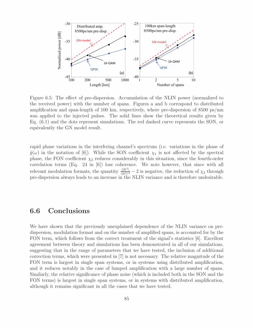
QPSK

16-QAM

GN-model

100km span-length

8500ps/nm pre-disp.

(b)

1040-

35-

30-

-25

Number of spans

521

QPSK

16-QAM

GN-model

Distributed amp.

8500ps/nm pre-disp.

No

rmal

ized

po

wer

[d

B]

(a)

1000

40-

35-

-30

Length [km]

50020010045-

Figure 6.5: The effect of pre-dispersion. Accumulation of the NLIN power (normalized tothe received power) with the number of spans. Figures a and b correspond to distributedamplification and span-length of 100 km, respectively, where pre-dispersion of 8500 ps/nmwas applied to the injected pulses. The solid lines show the theoretical results given byEq. (6.1) and the dots represent simulations. The red dashed curve represents the SON, orequivalently the GN model result.

rapid phase variations in the interfering channel’s spectrum (i.e. variations in the phase ofg(ω) in the notation of [6]). While the SON coefficient χ1 is not affected by the spectralphase, the FON coefficient χ2 reduces considerably in this situation, since the fourth-ordercorrelation terms (Eq. 24 in [6]) lose coherence. We note however, that since with all

relevant modulation formats, the quantity 〈|b|4〉〈|b|2〉2 − 2 is negative, the reduction of χ2 through

pre-dispersion always leads to an increase in the NLIN variance and is therefore undesirable.

6.6 Conclusions

We have shown that the previously unexplained dependence of the NLIN variance on pre-dispersion, modulation format and on the number of amplified spans, is accounted for by theFON term, which follows from the correct treatment of the signal’s statistics [6]. Excellentagreement between theory and simulations has been demonstrated in all of our simulations,suggesting that in the range of parameters that we have tested, the inclusion of additionalcorrection terms, which were presented in [7] is not necessary. The relative magnitude of theFON term is largest in single span systems, or in systems using distributed amplification,and it reduces notably in the case of lumped amplification with a large number of spans.Similarly, the relative significance of phase noise (which is included both in the SON and theFON terms) is largest in single span systems, or in systems with distributed amplification,although it remains significant in all the cases that we have tested.

85

6.7 Appendix: Computation of χ1 and χ2

The extraction of the analytical curves in Figs. 6.1 and 6.3 –6.5 relies on the computationof the SON and FON coefficients χ1 and χ2, which requires summation over three andfive indices, respectively. Multi-dimensional summations are extremely inefficient in brute-force computation, and hence we have adopted the Monte-Carlo integration method [13] forevaluating these quantities. We provide a code (written in Matlab) that computes χ1, χ2

(using Eqs. (26) and (27) of [6] including receiver matched filtering that removes productsthat fall outside of the received channel bandwidth), and allows the evaluation of the impliedNLIN variance according to Eq. (6.1). The program also evaluates the relative error in thecomputed NLIN variance, where in all of the numerical curves presented in this paper thenumber of integration points N was large enough to ensure that the relative error was wellunder 1%.

For the reader’s convenience, in addition to providing the tools for reproducing the curvespresented in this paper, we include blocks that compute the variance of nonlinear intra-channel noise, as well as additional inter-channel terms that contribute to NLIN when theguard-band between WDM channels is much smaller than the channel bandwidth, and whichwere first reported in [7]. It can be easily verified that the contribution of these terms isnegligible with the typical system parameters assumed in this paper, although they mayplay a role in the case of future densely spaced super-channels. The option of describing apolarization multiplexed link is also included. The program assumes perfect Nyquist pulsesand homogeneous fiber spans, but it can be readily extended to an arbitrary pulse-shapeand to systems with different span length and fiber dispersions.

The runtime for the computation of the SON and FON coefficients χ1 and χ2 on astandard PC with an i5 processor is of the order of 0.5 seconds, whereas the computation ofall (intra and inter-channel) NLIN terms is performed in less than 2 seconds. We note thatpolarization multiplexing does not affect the run-time of the code (although it more thandoubles the runtime of a full split-step simulation).

function main()%% System parametersclear; %clc;tic;PolMux = 0; % 0 when single polarization, 1 with polarization mulltiple xinggamma = 1.3; % Nonlinearity coefficient in [1/W/km]beta2 = 21; % Dispersion coefficient [psˆ2/km]alpha = 0.2; % Fiber loss coefficient [dB/km]Nspan = 24; % Number of spansL = 100; % Span length [km]PD = 0; % Pre−dispersion [psˆ2]PdBm = −2; % Average input power [dBm]BaudRate = 32; % Baud−rate [GHz]ChSpacing = 33.6; % Channel spacing [GHz]kur = 1; %1.32; % Second order modulation factor <|a|ˆ4 >/ <|a|ˆ2 >ˆ2kur3 = 1; %1.96; % Third order modulation factor <|a|ˆ6 >/ <|a|ˆ2 >ˆ3N = 1000000; % Number of integration points in algorithm [14]. Should

% be set such that the relative error is desirably small.

86

%% Monte−Carlo integrationalpha norm = alpha/10 * log(10);T=1000/BaudRate;P0 = 10ˆ((PdBm −30)/10);beta2 norm = beta2/Tˆ2;PD norm = PD/Tˆ2;ChSpacing norm = ChSpacing./BaudRate;

%% calculate inter −channel nonlinear noise variance according to Eq. (1)[NLIN var chi1 chi2 Err] = calc interChannel(gamma,beta2 norm,alpha norm, ...

Nspan,L,PD norm,P0,kur,kur3,N,PolMux,ChSpacing norm);

%% displaydisp( '%%%%%%%%%%%%%%%%%%%%%%%%%%%%%%%%%%%%%%%%%%%%%%');if (PolMux == 1)

disp( '%%%Polarization Multiplexed case is considered%%%' );enddisp( '%%Results correspond to a single interferer%%%' )disp([ '(1) chi 1 = ' num2str(chi1) ', chi 2 = ' num2str(chi2)]);disp([ '(2) NLIN variance according to Eq. (1) is ' num2str(NLIN var) ...

' Watts (' num2str(10 * log10(NLIN var * 1000)) 'dBm).' ...' Relative computation error is ' , num2str(Err * 100), '%' ]);

%% calculate the contribution of the additional inter −channel terms of [7]NLIN var addTerm = calc interChannel addTerms(gamma,beta2 norm,alpha norm, ...

Nspan,L,PD norm,P0,kur,kur3,N,PolMux,ChSpacing norm);

%% calculate intra −channel nonlinear noise%% NLINvar intra(1) is the intra −channel nonlinear noise variance%% NLINvar intra(2) is due to the nonlinear broadening of the adjacent i nterfererNLIN var intra = calc intraChannel(gamma,beta2 norm,alpha norm, ...

Nspan,L,PD norm,P0,kur,kur3,N,PolMux,ChSpacing norm);NLIN var addTerm = NLIN var addTerm + NLIN var intra(2);

%%Continue displaydisp([ '(3) Contribution of additional inter −channel interference ' ...

'terms of [7] is ' num2str(NLIN var addTerm) ' Watts (' ...num2str(10 * log10(NLIN var addTerm * 1000)) 'dBm)' ]);

disp([ '(4) Total NLIN variance (2)+(3) is ' num2str(NLIN var+NLIN var addTerm) ...' Watts (' num2str(10 * log10((NLIN var+NLIN var addTerm) * 1000)) 'dBm)' ]);

disp([ '(5) Intra −Channel nonlinear noise variance is ' num2str(NLIN var intra(1)) ...' Watts (' num2str(10 * log10(NLIN var intra(1) * 1000)) 'dBm)' ]);

toc;disp( '%%%%%%%%%%%%%%%%%%%%%%%%%%%%%%%%%%%%%%%%%%%%%%');end

%%%%%%%%%%%%%%%%%%%%%%%%%function [NLIN var chi1 chi2 Err] = ...

calc interChannel(gamma,beta2,alpha,Nspan,L,PD,P0,kur,ku r3,N,PolMux,q)

R = 2* pi * (rand(4, N) −0.5 * ones(4, N));Volume = (2 * pi)ˆ4;

87

%% calculate chi1w0 = R(1,:) −R(2,:)+R(3,:);arg1 = (R(2,:) −R(3,:)). * (R(2,:)+2 * pi * q−R(1,:));argPD1 = arg1;ss1 = exp(1i * argPD1 * PD). * (exp(1i * beta2 * arg1 * L−alpha * L) −1) ...

./(1i * beta2 * arg1 −alpha). * (w0<pi). * (w0>−pi);s1 = abs(ss1. * (1 −exp(1i * Nspan* arg1 * beta2 * L)) ...

./(1 −exp(1i * arg1 * beta2 * L))).ˆ2/Volume;avgF1 = sum(s1)/N;chi1 = avgF1 * Volume * (4 * gammaˆ2* P0ˆ3);

%% calculate chi2w3p = −R(2,:)+R(4,:)+R(3,:)+2 * pi * q;arg2 = (R(2,:) −R(3,:)). * (R(4,:) −R(1,:)+2 * pi * q);argPD2 = arg2;ss2 = exp( −1i * argPD2 * PD). * (exp( −1i * beta2 * arg2 * L−alpha * L) −1) ...

./( −1i * beta2 * arg2 −alpha). * (w3p>−pi+2 * pi * q). * (w3p<pi+2 * pi * q);s2 = (1 −exp(1i * Nspan* arg1 * beta2 * L))./(1 −exp(1i * arg1 * beta2 * L)). * ss1 ...

. * (1 −exp( −1i * Nspan* arg2 * beta2 * L)) ...

./(1 −exp( −1i * arg2 * beta2 * L)). * ss2/Volume;avgF2 = real(sum(s2))/N;chi2 = avgF2 * Volume * (4 * gammaˆ2* P0ˆ3);

%% calculate NLINNLIN var = chi1+(kur −2) * chi2;if (PolMux == 1)

NLIN var = (9/8)ˆ2 * 16/81 * (NLIN var+2 * chi1/4+(kur −2) * chi2/4);end

%% calculate the root mean square relative errorif (PolMux == 0)

Err = (sum((s1 −avgF1+(kur −2) * (real(s2) −avgF2)).ˆ2) .../(N −1)) .4/(avgF1+(kur −2) * avgF2)/sqrt(N);

elseErr = (sum(((9/8)ˆ2 * 16/81 * (6/4 * (s1 −avgF1)+5/4 * (kur −2) * ...

(real(s2) −avgF2))).ˆ2)/(N −1)) .4/((9/8)ˆ2 * 16/81 * ...(6/4 * avgF1+5/4 * (kur −2) * avgF2))/sqrt(N);

end

end

%%%%%%%%%%%%%%%%%%%%%%%%%function [NLIN var] = calc interChannel addTerms(gamma,beta2,alpha, ...

Nspan,L,PD,P0,kur,kur3,N,PolMux,q)

R = 2* pi * (rand(4, N) −0.5 * ones(4, N));

%% calculate X21w0 = R(1,:) −R(2,:)+R(3,:)+2 * pi * q;arg1 = (R(2,:) −R(3,:) −2* pi * q). * (R(2,:) −R(1,:));argPD1 = arg1;ss1 = exp(1i * argPD1 * PD). * (exp(1i * beta2 * arg1 * L−alpha * L) −1) ...

./(1i * beta2 * arg1 −alpha). * (w0<pi). * (w0>−pi);s1 = abs(ss1. * (1 −exp(1i * Nspan* arg1 * beta2 * L))./(1 −exp(1i * arg1 * beta2 * L))).ˆ2;

88

X21 = sum(s1) * (gammaˆ2 * P0ˆ3)/N;

%% calculate X22w1 = R(1,:) −R(2,:)+R(4,:);arg2 = (w1 −R(3,:) −2* pi * q). * (R(2,:) −R(1,:));argPD2 = arg2;ss2 = exp( −1i * argPD2 * PD). * (exp( −1i * beta2 * arg2 * L−alpha * L) −1) ...

./( −1i * beta2 * arg2 −alpha). * (w1<pi). * (w1>−pi);s2 = (1 −exp(1i * Nspan* arg1 * beta2 * L))./(1 −exp(1i * arg1 * beta2 * L)). * ss1 ...

. * (1 −exp( −1i * Nspan* arg2 * beta2 * L))./(1 −exp( −1i * arg2 * beta2 * L)). * ss2;X22 = real(sum(s2)) * (gammaˆ2 * P0ˆ3)/N;

%% calculate X23w2 = R(1,:)+R(2,:) −R(3,:) −2* pi * q;arg1 = (R(3,:)+2 * pi * q−R(2,:)). * (R(3,:)+2 * pi * q−R(1,:));argPD1 = arg1;ss3 = exp(1i * argPD1 * PD). * (exp(1i * beta2 * arg1 * L−alpha * L) −1) ...

./(1i * beta2 * arg1 −alpha). * (w2<pi). * (w2>−pi);s3 = abs(ss3. * (1 −exp(1i * Nspan* arg1 * beta2 * L))./(1 −exp(1i * arg1 * beta2 * L))).ˆ2;X23 = sum(s3) * (gammaˆ2 * P0ˆ3)/N;

%% calculate X24w3 = R(1,:) −R(4,:)+R(2,:);arg2 = (R(3,:)+2 * pi * q−R(4,:)). * (R(3,:)+2 * pi * q−w3);argPD2 = arg2;ss4 = exp( −1i * argPD2 * PD). * (exp( −1i * beta2 * arg2 * L−alpha * L) −1) ...


. * (1 −exp( −1i * Nspan* arg2 * beta2 * L))./(1 −exp( −1i * arg2 * beta2 * L)). * ss4;X24 = real(sum(s4)) * (gammaˆ2 * P0ˆ3)/N;

%% calculate NLINNLIN var = 4 * X21+4* (kur −2) * X22+2* X23+(kur −2) * X24;if (PolMux == 1)

NLIN var = (9/8)ˆ2 * 16/81 * (NLIN var+2 * X21+(kur −2) * X22+X23+0* (kur −2) * X24);end

end

%%%%%%%%%%%%%%%%%%%%%%%%%function [NLIN var] = ...

calc intraChannel(gamma,beta2,alpha,Nspan,L,PD,P0,kur,ku r3,N,PolMux,q)

if (exist( 'q' )==0) q = 0; end ;R = 2* pi * (rand(5, N) −0.5 * ones(5, N));

%% calculate X1w0 = R(1,:) −R(2,:)+R(3,:);argInB = (w0 <pi). * (w0>−pi);argOutB = (w0 <pi+2 * pi * q). * (w0>−pi+2 * pi * q);arg1 = (R(2,:) −R(3,:)). * (R(2,:) −R(1,:));argPD1 = arg1;ss1 = exp(1i * argPD1 * PD). * (exp(1i * beta2 * arg1 * L−alpha * L) −1) ...

./(1i * beta2 * arg1 −alpha);

89

s1 = abs(ss1. * (1 −exp(1i * Nspan* arg1 * beta2 * L))./(1 −exp(1i * arg1 * beta2 * L))).ˆ2;X1 = [sum(s1. * argInB) sum(s1. * argOutB)] * (gammaˆ2 * P0ˆ3)./N;

%% calculate X0s0 = ss1. * (1 −exp(1i * Nspan* arg1 * beta2 * L))./(1 −exp(1i * arg1 * beta2 * L));X0 = [abs(sum(s0. * argInB)/N).ˆ2 abs(sum(s0. * argOutB)/N).ˆ2] * (gammaˆ2 * P0ˆ3);

%% calculate X2w1 = −R(2,:)+R(4,:)+R(3,:);arg2 = (R(2,:) −R(3,:)). * (R(4,:) −R(1,:));argPD2 = arg2;ss2 = exp( −1i * argPD2 * PD). * (exp( −1i * beta2 * arg2 * L−alpha * L) −1) ...


. * (1 −exp( −1i * Nspan* arg2 * beta2 * L))./(1 −exp( −1i * arg2 * beta2 * L)). * ss2;X2 = [real(sum(s2. * argInB)) real(sum(s2. * argOutB))] * (gammaˆ2 * P0ˆ3)./N;

%% calculate X21w2 = R(4,:) −R(1,:) −R(3,:);arg2 = (R(2,:) −R(4,:)). * (R(2,:) −w2);argPD2 = arg2;ss2 = exp( −1i * argPD2 * PD). * (exp( −1i * beta2 * arg2 * L−alpha * L) −1) ...



%% calculate X3w3 = R(1,:) −R(2,:)+R(4,:)+R(3,:) −R(5,:);arg3 = (R(4,:) −R(5,:)). * (R(4,:) −w3);argPD3 = arg3;ss3 = exp( −1i * argPD3 * PD). * (exp( −1i * beta2 * arg3 * L−alpha * L) −1) ...



%% calculate NLINNLIN var = 2 * X1+(kur −2) * (4 * X2+X21)+(kur3 −9* kur+12) * X3−(kur −2)ˆ2 * X0;if (PolMux == 1)

NLIN var = (9/8)ˆ2 * 16/81 * (NLIN var+X1+(kur −2) * X2);end

end

Acknowledgment

The authors would like to acknowledge financial support from the Israel Science Foundation(grant 737/12). Ronen Dar would like to acknowledge the support of the Adams Fellowship ofthe Israel Academy of Sciences and Humanities, the Yitzhak and Chaya Weinstein ResearchInstitute, and the Feder Family Award.

90

Bibliography

[1] R.-J. Essiambre, G. Kramer, P.J. Winzer, G.J. Foschini, B. Goebel, “Capacity limits ofoptical fiber networks,” J. Lightwave Technol. 28, 662–701 (2010).

[2] P. Poggiolini, A. Carena, V. Curri, G. Bosco, F. Forghieri, “Analytical modeling ofnonlinear propagation in uncompensated optical transmission links,” IEEE Photon.Technol. Lett. 23, 742–744 (2011).

[3] A. Carena, V. Curri, G. Bosco, P. Poggiolini, F. Forghieri, “Modeling of the impact ofnonlinear propagation effects in uncompensated optical coherent transmission links,” J.Lightwave Technol. 30, 1524–1539 (2012).

[4] A. Carena, G. Bosco, V. Curri, P. Poggiolini, F. Forghieri, “Impact of the transmittedsignal initial dispersion transient on the accuracy of the GN-model of non-linear propa-gation,” 39th European Conference and Exhibition on Optical Communication (ECOC2013), Paper Th.1.D.4.

[5] P. Johannisson and M. Karlsson, “Perturbation analysis of nonlinear propagation ina strongly dispersive optical communication system,” IEEE J. Lightwave Technol. 31,1273–1282 (2013).

[6] R. Dar, M. Feder, A. Mecozzi, M. Shtaif, “Properties of nonlinear noise in long,dispersion-uncompensated fiber links,” Optics Express, 21, pp. 25685–25699 (2013).

[7] A. Carena, G. Bosco, V. Curri, Y. Jiang, P. Poggiolini, F. Forghieri, “On the accuracyof the GN-model and on analytical correction terms to improve it,” arXiv preprint1401.6946v1 (2014).

[8] A. Mecozzi and R.-J. Essiambre, “Nonlinear Shannon limit in pseudolinear coherentsystems,” J. Lightwave Technol. 30, 2011–2024 (2012).

[9] M. Secondini, E. Forestieri, G. Prati, “Achievable information rate in nonlinear WDMfiber-optic systems with arbitrary modulation formats and dispersion maps,” J. Light-wave Technol. 31, 3839–3852 (2013).

[10] R. Dar, M. Shtaif, M. Feder, “New bounds on the capacity of the nonlinear fiber-opticchannel,” Optics Lett. 39, 398–401 (2014).

[11] J. P. Gordon and L. F. Mollenauer, “Effects of fiber nonlinearities and amplifier spacingon ultra-long distance transmission,” J. Lightwave Technol. 9, 170–173 (1991)

91

[12] M. Shtaif, “Analytical description of cross-phase modulation in dispersive optical fibers.”Optics Lett. 23, 1191–1193 (1998).

[13] R. E. Caflisch, “Monte Carlo and quasi-Monte Carlo methods,” Acta Numerica 7, Cam-bridge University Press, 1–49 (1998).

92

Chapter 7

Inter-Channel Nonlinear Interference

Noise in WDM Systems: Modeling

and MitigationRonen Dar, Meir Feder, Antonio Mecozzi and Mark Shtaif, “Inter-channel nonlinear inter-ference noise in WDM systems: modeling and mitigation,” invited paper, IEEE Journal ofLightwave Technology, vol. 33, pp. 1044–1053 (March 2015)

7.1 Abstract

We review the modeling of inter-channel nonlinear interference noise (NLIN) in fiber-opticcommunication systems, focusing on the accurate extraction of the NLIN variance, the depen-dence on modulation format, the role of nonlinear phase-noise and the existence of temporalcorrelations. We show ways in which temporal correlations can be exploited for reducing theimpact of NLIN, and discuss the prospects of this procedure in future systems.

7.2 Introduction

Signal distortions imposed by the nonlinearity of optical fibers are arguably the most sig-nificant factor limiting the capacity of modern wavelength division multiplexed (WDM)communications systems [1,2]. Nonlinear distortions are customarily categorized as belong-ing to the intra-channel [3] or the inter-channel [4] types. Intra-channel distortions are thoseaffecting an individual WDM channel independently of the other WDM channels propa-gating in the fiber. Inter-channel distortions are those in which a given WDM channel isaffected by the electric fields of the neighboring WDM channels that propagate in the fiberat the same time. In principle, while intra-channel distortions can be eliminated by means ofdigital back propagation at the receiver [5], or pre-distortion at the transmitter [6], similarelimination of inter-channel distortions is considered impractical. The difficulty is not onlyin the need of coherently detecting and jointly processing multiple WDM channels, but alsobecause of the unpredictable add-drop operations taking place in modern optical networks,and the fact that the polarizations states of different WDM channels evolve randomly and

93

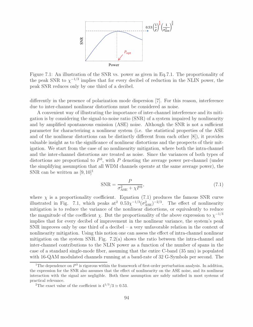
0.531 1

Power

SN

R

Figure 7.1: An illustration of the SNR vs. power as given in Eq.7.1. The proportionality ofthe peak SNR to χ−1/3 implies that for every decibel of reduction in the NLIN power, thepeak SNR reduces only by one third of a decibel.

differently in the presence of polarization mode dispersion [7]. For this reason, interferencedue to inter-channel nonlinear distortions must be considered as noise.

A convenient way of illustrating the importance of inter-channel interference and its miti-gation is by considering the signal-to-noise ratio (SNR) of a system impaired by nonlinearityand by amplified spontaneous emission (ASE) noise. Although the SNR is not a sufficientparameter for characterizing a nonlinear system (i.e. the statistical properties of the ASEand of the nonlinear distortions can be distinctly different from each other [8]), it providesvaluable insight as to the significance of nonlinear distortions and the prospects of their mit-igation. We start from the case of no nonlinearity mitigation, where both the intra-channeland the inter-channel distortions are treated as noise. Since the variances of both types ofdistortions are proportional to P 3, with P denoting the average power per-channel (underthe simplifying assumption that all WDM channels operate at the same average power), theSNR can be written as [9, 10]1

SNR =P

σ2ASE + χP 3

, (7.1)

where χ is a proportionality coefficient. Equation (7.1) produces the famous SNR curveillustrated in Fig. 7.1, which peaks at2 0.53χ−1/3(σ2

ASE)−2/3. The effect of nonlinearity

mitigation is to reduce the variance of the nonlinear distortions, or equivalently to reducethe magnitude of the coefficient χ. But the proportionality of the above expression to χ−1/3

implies that for every decibel of improvement in the nonlinear variance, the system’s peakSNR improves only by one third of a decibel – a very unfavorable relation in the context ofnonlinearity mitigation. Using this notion one can assess the effect of intra-channel nonlinearmitigation on the system SNR. Fig. 7.2(a) shows the ratio between the intra-channel andinter-channel contributions to the NLIN power as a function of the number of spans in thecase of a standard single-mode fiber, assuming that the entire C-band (35 nm) is populatedwith 16-QAM modulated channels running at a baud-rate of 32 G-Symbols per second. The

1The dependence on P 3 is rigorous within the framework of first-order perturbation analysis. In addition,the expression for the SNR also assumes that the effect of nonlinearity on the ASE noise, and its nonlinearinteraction with the signal are negligible. Both these assumption are safely satisfied in most systems ofpractical relevance.

2The exact value of the coefficient is 41/3/3 ≃ 0.53.

94

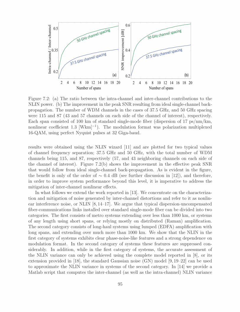
Intr

a-c

hannel

/In

ter-

ch

ann

el

Number of spans

(a)

0.5

0.35

0.2

8642 16141210 2018

SN

R i

mp

rov

em

en

t [d

B]

Number of spans

(b)

0.6

0.4

0.2

8642 16141210 2018

Figure 7.2: (a) The ratio between the intra-channel and inter-channel contributions to theNLIN power. (b) The improvement in the peak SNR resulting from ideal single-channel back-propagation. The number of WDM channels in the cases of 37.5 GHz, and 50 GHz spacingwere 115 and 87 (43 and 57 channels on each side of the channel of interest), respectively.Each span consisted of 100 km of standard single-mode fiber (dispersion of 17 ps/nm/km,nonlinear coefficient 1.3 [Wkm]−1). The modulation format was polarization multiplexed16-QAM, using perfect Nyquist pulses at 32 Giga-baud.

results were obtained using the NLIN wizard [11] and are plotted for two typical valuesof channel frequency separation; 37.5 GHz and 50 GHz, with the total number of WDMchannels being 115, and 87, respectively (57, and 43 neighboring channels on each side ofthe channel of interest). Figure 7.2(b) shows the improvement in the effective peak SNRthat would follow from ideal single-channel back-propagation. As is evident in the figure,the benefit is only of the order of ∼ 0.4 dB (see further discussion in [12]), and therefore,in order to improve system performance beyond this level, it is imperative to address themitigation of inter-channel nonlinear effects.

In what follows we extend the work reported in [13]. We concentrate on the characteriza-tion and mitigation of noise generated by inter-channel distortions and refer to it as nonlin-ear interference noise, or NLIN [8, 14–17]. We argue that typical dispersion-uncompensatedfiber-communications links installed over standard single-mode fiber can be divided into twocategories. The first consists of metro systems extending over less than 1000 km, or systemsof any length using short spans, or relying mostly on distributed (Raman) amplification.The second category consists of long-haul systems using lumped (EDFA) amplification withlong spans, and extending over much more than 1000 km. We show that the NLIN in thefirst category of systems exhibits clear phase-noise-like features and a strong dependence onmodulation format. In the second category of systems these features are suppressed con-siderably. In addition, while in the first category of systems, the accurate assessment ofthe NLIN variance can only be achieved using the complete model reported in [8], or itsextension provided in [18], the standard Gaussian noise (GN) model [9, 19–22] can be usedto approximate the NLIN variance in systems of the second category. In [14] we provide aMatlab script that computes the inter-channel (as well as the intra-channel) NLIN variance

95

within seconds. The implementation of this script with a number of important extensions isalso available as an online application at [11].

Another topic that we address in this paper is the correlation properties of inter-channelNLIN [8, 15–17], which offer a potential path for inter-channel nonlinearity mitigation. Thepresence of chromatic dispersion causes different WDM channels to propagate at differentgroup velocities, so that every symbol in the channel of interest interacts with multiplesymbols of every interfering channel. Consequently, adjacent symbols in the channel ofinterest are disturbed by essentially the same collection of interfering pulses, and are thereforeaffected by nonlinearity in a highly correlated manner 3. This property has been exploitedto some extent in [15], where it was shown that when taking this correlation into accountwith respect to the phase-noise component of NLIN, the lower bound for the informationcapacity increases by nearly 1 bit. The implications of temporal correlations on the channelcapacity have also been recently considered in [25]. We take this idea further and arguethat a channel impaired by inter-channel NLIN is equivalent to a linear channel with time-varying inter-symbol interference (ISI) [16,17,26]. Using this concept, we evaluate the extentto which mitigation of inter-channel nonlinearities may improve system performance.

The paper is organized as follows. In Sec. 7.3 we briefly review the essentials of thetime domain model, initially introduced in [8, 27], and extend the main equations to thepolarization multiplexed case. In Sec. 7.4 we quantify the significance of modulation formatdependence and the phase-noise-like nature of NLIN in polarization multiplexed systems. InSec. 7.5 we introduce the time-varying ISI model and evaluate the potential of inter-channelNLIN mitigation. Finally, Sec. 7.6 is devoted to conclusions.

7.3 NLIN modeling

Throughout this work we neglect the effect of four-wave-mixing, whose significance in thekind of systems used in modern communications (particularly when implemented over stan-dard single-mode fiber (SMF)) is known to be secondary, and focus our attention on in-terference due to the cross-phase-modulation (XPM) effect. Since this effect only involvestwo-channel interactions, the NLIN contributions of multiple WDM channels add up inde-pendently, and hence we conduct the initial analysis with only two channels, one of which isthe channel of interest (whose central frequency is arbitrarily set to 0) and the other is theinterfering channel, and its central frequency is denoted by Ω. The electric field vector thatis injected into the fiber is thereby given by4

u(0, t) =∑

n

ang(0, t− nT ) + e−iΩt∑

n

bng(0, t− nT ) , (7.2)

3The existence of temporal correlations can also be seen from the power spectral density of NLIN, whichhas been considered in [23, 24].

4For simplicity, Eq. (7.2) assumes that the modulated polarization axes of the interacting channels areparallel to each other. While this assumption significantly simplifies the analysis it does not affect theresults presented in this paper. In particular, the NLIN power and its dependence on modulation formatare independent of the relative rotation between the channels. The magnitude of phase-noise may changewith the the relative orientation of the channels, but the major conclusions regarding the significance ofphase-noise and its dependence on modulation format remain valid.

96

where the symbols an and bn represent the transmitted data in the channel of interest andinterfering channel, respectively, in the n-th time-slot, and T is the symbol duration. Theunderlined quantities in Eq. (7.2) and throughout this paper are column vectors, whosetwo elements correspond to the two polarization components of the field. The injectedfundamental symbol waveform is denoted by g(0, t) and it is assumed to be normalized inenergy and orthogonal with respect to time shifts by an integer number of symbol durations,i.e.

∫g∗(0, t − nT )g(0, t − n′T )dt = δn,n′. The dispersed waveform of the individual pulse

when reaching point z along the fiber is g(z, t) = exp(− i2β ′′z ∂2

∂t2)g(0, t), where β ′′ is the fiber

dispersion coefficient5.We now focus, without loss of generality, on the detection of the zeroth-index data sym-

bols a0. We assume coherent detection preceded by a matched filter that isolates the channelof interest and removes the effect of chromatic dispersion. We note that throughout this workwe assume a matched filter that is optimized to the unperturbed system, namely one withoutthe nonlinear interference. The received signal samples in the two polarizations can then beexpressed as r0 = a0 +∆a0, where ∆a0 represents the NLIN contribution. It can be shownthat within the first order perturbation analysis [27], the results of [8, 27] can be readilyextended to the two-polarization case, yielding

∆a0 = i8

9γ∑

l,k,m

Sl,k,ma†kamal

+i8

9γ∑

l,k,m

Xl,k,m(b†kbmI+ bmb

†k)al, (7.3)

where γ is the fiber’s nonlinearity coefficient, I is a 2×2 identity matrix, and the coefficientsSl,k,m and Xl,k,m are given by

Sl,k,m=

∫ L

0

dzf(z)

∫ ∞

−∞dt g∗(z, t)g(z, t− lT )

×g∗(z, t− kT )g(z, t−mT ) (7.4)

and

Xl,k,m=

∫ L

0

dzf(z)

∫ ∞

−∞dt g∗(z, t)g(z, t− lT )

×g∗(z, t−kT − β ′′Ωz)g(z, t−mT − β ′′Ωz). (7.5)

Here L is the length of the link and the function f(z) accounts for its loss/gain profile. Forexample, it is equal to 1 in the case of perfectly distributed amplification and f(z) = exp(−αmod(z, Ls)) in the case of lumped amplification (where α is the loss coefficient, Ls is the span-length, and where mod(z, Ls) is the modulo operation). The first and second summationson the right-hand side of Eq. (7.3) represent intra-channel and inter-channel interference,respectively. As mentioned earlier, we shall focus in what follows on the NLIN due to inter-channel interactions and ignore the terms proportional to Sl,k,m.

5Note the change in notation with respect to [8], where the waveform which we now denote by g(z, t) wasdenoted by g(0)(z, t).

97

Equation (7.3) illuminates two relevant features of NLIN, whose significance will be quan-tified in Sec. 7.4. These are the existence of a phase-noise component within the NLIN andthe dependence of the NLIN on the modulation format of the interfering channels. The phase-noise contribution arrives from the diagonal elements of the 2×2 matricesX0,k,m(b

†kbmI+bmb

†k)

corresponding to l = 0. These contributions can be divided into two subgroups. The firstsubgroup (which constitutes the largest contribution to phase-noise [8,28]) consists of termswhere k = m, whereas the second subgroup consists of the terms where k andm are different.Since the coefficients X0,m,m can be readily seen to be real-valued, the diagonal contribu-tions from the first group are at a complex angle of π/2 from the detected symbol a0, andhence they constitute phase-noise. A similar conclusion can be drawn for the terms in whichk 6= m, when noting that X0,k,m = X∗

0,m,k and after summing the contributions in which kand m are permuted with each other.

The dependence of the NLIN on modulation format follows from the terms in Eq. (7.3)where k = m. This dependence is particularly significant to the magnitude of the phase-noise part of NLIN, which (as mentioned earlier) is dominated by this kind of terms. Indeed,when the interfering channel is phase-modulated (e.g. QPSK), the phase-noise experiencedby the channel of interest has been demonstrated [8,14] to be much smaller than it is whenthe amplitude of the interfering channel is modulated as well. The dependence of the overallinter-channel NLIN variance on modulation format has been explored in [8], where it hasbeen shown that when the symbols transmitted over the two channels are independent,identically and isotropically distributed, this variance can be expressed as

σ2NLIN = P 3χ1

︸︷︷︸SON\GN

+P 3χ2

( 〈|b|4〉〈|b|2〉2 − 2

)

︸︷︷︸FON

, (7.6)

where P is the average input power (assuming it is equal in bothWDM channels), b representsa single-polarization constellation point of the interfering channel, and the angled bracketsdenote statistical averaging over the data constellation points6. The terms χ1 and χ2 in asingle-polarization transmission are given by Eqs. (26) and (27) in [8] (multiplied by T 3),whereas in the case of dual polarizations they need to be multiplied by 8/27 and 20/81,respectively. In the appendix of this paper we provide a time-domain representation forthese terms and illustrate the relation with the frequency domain analysis adopted in [8].

The first term on the right-hand-side of (7.6) is identical to the value that the GNmodel [9, 19, 20] assigns to the variance of the inter-channel NLIN, and since it follows onlyfrom second-order statistics, we refer to it as the second-order noise (SON) term. The secondterm depends on fourth-order statistics and is hence referred to as the fourth-order noise(FON) term. The presence of the fourth moment 〈|b|4〉 in the FON term is responsible forthe dependence on modulation format. The value of (〈|b|4〉/〈|b|2〉2 − 2) is −1,−1.32,−1.38and 0 for the cases of QPSK, 16-QAM, 64-QAM, and Gaussian modulation, respectively.Note that only with Gaussian modulation the second term in Eq. (7.6) vanishes and theresult of the GN model becomes exact.

6As is customary in the fiber-optics community, P represents the total average signal power (over bothpolarizations) and σ2

NLIN is the sum of the NLIN variances in the two polarizations. It is assumed thatthe symbols transmitted over the two polarizations are statistically independent of each other and that themodulation formats are identical.

98

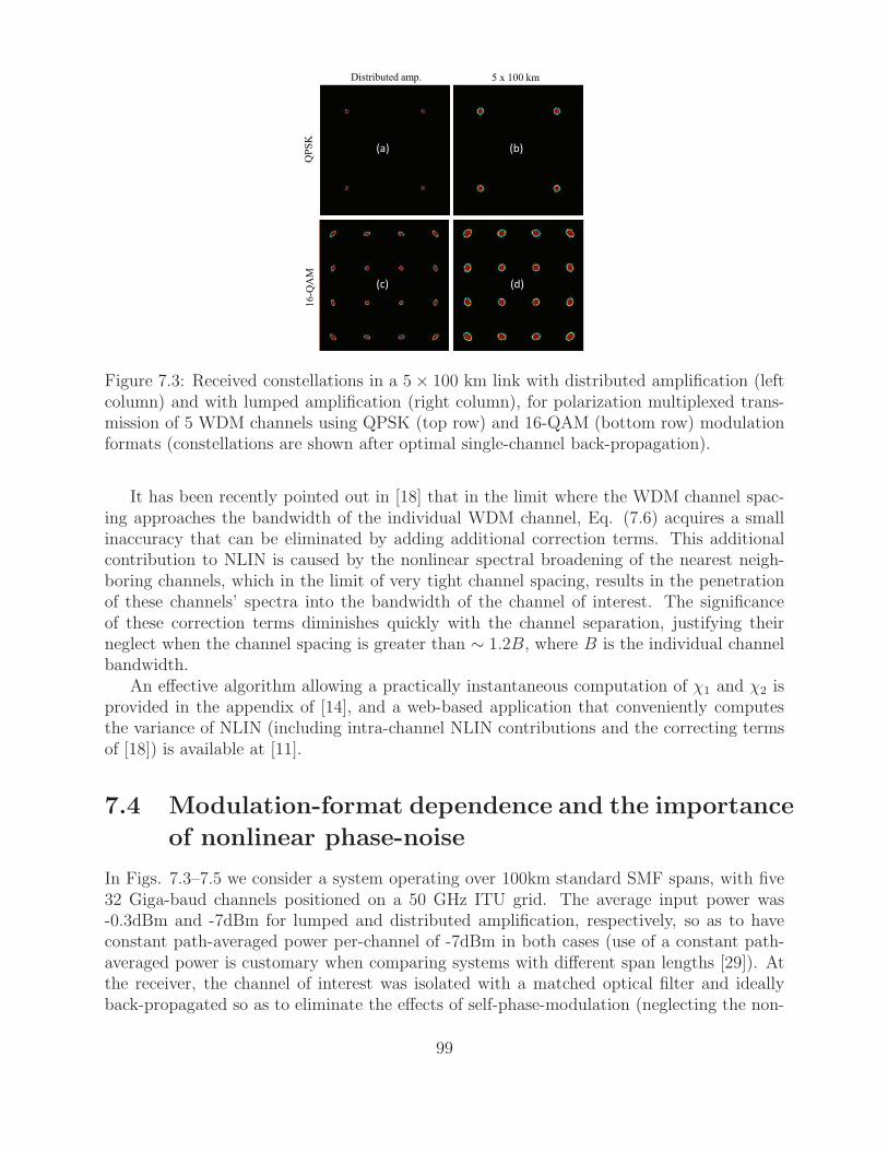
16

-QA

MQ

PS

K

Distributed amp. 5 x 100 km

(a) (b)

(c) (d)

Figure 7.3: Received constellations in a 5× 100 km link with distributed amplification (leftcolumn) and with lumped amplification (right column), for polarization multiplexed trans-mission of 5 WDM channels using QPSK (top row) and 16-QAM (bottom row) modulationformats (constellations are shown after optimal single-channel back-propagation).

It has been recently pointed out in [18] that in the limit where the WDM channel spac-ing approaches the bandwidth of the individual WDM channel, Eq. (7.6) acquires a smallinaccuracy that can be eliminated by adding additional correction terms. This additionalcontribution to NLIN is caused by the nonlinear spectral broadening of the nearest neigh-boring channels, which in the limit of very tight channel spacing, results in the penetrationof these channels’ spectra into the bandwidth of the channel of interest. The significanceof these correction terms diminishes quickly with the channel separation, justifying theirneglect when the channel spacing is greater than ∼ 1.2B, where B is the individual channelbandwidth.

An effective algorithm allowing a practically instantaneous computation of χ1 and χ2 isprovided in the appendix of [14], and a web-based application that conveniently computesthe variance of NLIN (including intra-channel NLIN contributions and the correcting termsof [18]) is available at [11].

7.4 Modulation-format dependence and the importance

of nonlinear phase-noise

In Figs. 7.3–7.5 we consider a system operating over 100km standard SMF spans, with five32 Giga-baud channels positioned on a 50 GHz ITU grid. The average input power was-0.3dBm and -7dBm for lumped and distributed amplification, respectively, so as to haveconstant path-averaged power per-channel of -7dBm in both cases (use of a constant path-averaged power is customary when comparing systems with different span lengths [29]). Atthe receiver, the channel of interest was isolated with a matched optical filter and ideallyback-propagated so as to eliminate the effects of self-phase-modulation (neglecting the non-

99

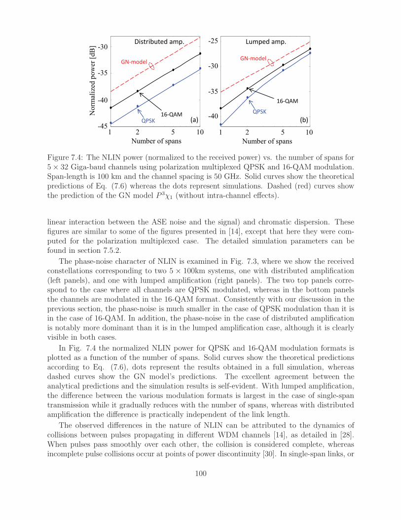
No

rmal

ized

po

wer

[d

B]

QPSK16-QAM

GN-model

Distributed amp.

(a)

10

40-

35-

-30

Number of spans

52145-

10

40-

35-

30-

-25

Number of spans

521

GN-model

QPSK

16-QAM

Lumped amp.

(b)

Figure 7.4: The NLIN power (normalized to the received power) vs. the number of spans for5× 32 Giga-baud channels using polarization multiplexed QPSK and 16-QAM modulation.Span-length is 100 km and the channel spacing is 50 GHz. Solid curves show the theoreticalpredictions of Eq. (7.6) whereas the dots represent simulations. Dashed (red) curves showthe prediction of the GN model P 3χ1 (without intra-channel effects).

linear interaction between the ASE noise and the signal) and chromatic dispersion. Thesefigures are similar to some of the figures presented in [14], except that here they were com-puted for the polarization multiplexed case. The detailed simulation parameters can befound in section 7.5.2.

The phase-noise character of NLIN is examined in Fig. 7.3, where we show the receivedconstellations corresponding to two 5 × 100km systems, one with distributed amplification(left panels), and one with lumped amplification (right panels). The two top panels corre-spond to the case where all channels are QPSK modulated, whereas in the bottom panelsthe channels are modulated in the 16-QAM format. Consistently with our discussion in theprevious section, the phase-noise is much smaller in the case of QPSK modulation than it isin the case of 16-QAM. In addition, the phase-noise in the case of distributed amplificationis notably more dominant than it is in the lumped amplification case, although it is clearlyvisible in both cases.

In Fig. 7.4 the normalized NLIN power for QPSK and 16-QAM modulation formats isplotted as a function of the number of spans. Solid curves show the theoretical predictionsaccording to Eq. (7.6), dots represent the results obtained in a full simulation, whereasdashed curves show the GN model’s predictions. The excellent agreement between theanalytical predictions and the simulation results is self-evident. With lumped amplification,the difference between the various modulation formats is largest in the case of single-spantransmission while it gradually reduces with the number of spans, whereas with distributedamplification the difference is practically independent of the link length.

The observed differences in the nature of NLIN can be attributed to the dynamics ofcollisions between pulses propagating in different WDM channels [14], as detailed in [28].When pulses pass smoothly over each other, the collision is considered complete, whereasincomplete pulse collisions occur at points of power discontinuity [30]. In single-span links, or

100

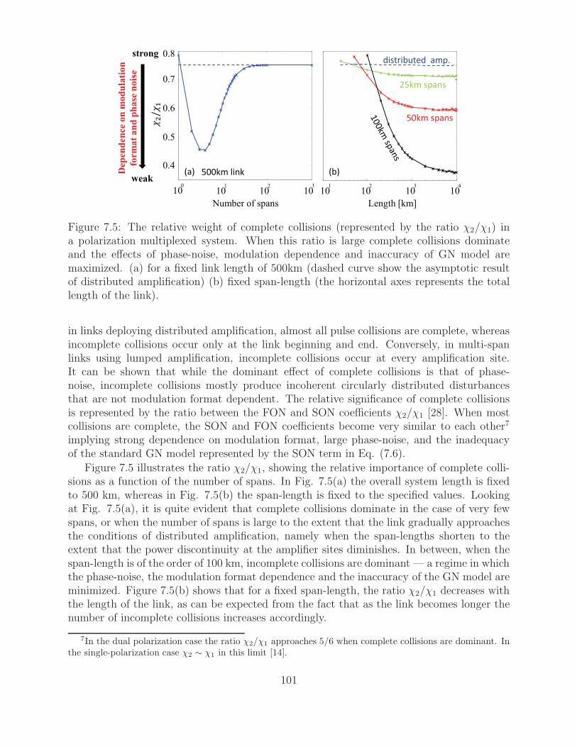
strong

weak

Dep

end

ence

on

mo

du

lati

on

form

at

an

d p

ha

se n

ois

e

101

0.5

0.6

0.7

0.8

102

103

104

Length [km]

0.4

100

101

102

103

Number of spans

50km spans

25km spans

distributed amp.

/

(a) (b)500km link

Figure 7.5: The relative weight of complete collisions (represented by the ratio χ2/χ1) ina polarization multiplexed system. When this ratio is large complete collisions dominateand the effects of phase-noise, modulation dependence and inaccuracy of GN model aremaximized. (a) for a fixed link length of 500km (dashed curve show the asymptotic resultof distributed amplification) (b) fixed span-length (the horizontal axes represents the totallength of the link).

in links deploying distributed amplification, almost all pulse collisions are complete, whereasincomplete collisions occur only at the link beginning and end. Conversely, in multi-spanlinks using lumped amplification, incomplete collisions occur at every amplification site.It can be shown that while the dominant effect of complete collisions is that of phase-noise, incomplete collisions mostly produce incoherent circularly distributed disturbancesthat are not modulation format dependent. The relative significance of complete collisionsis represented by the ratio between the FON and SON coefficients χ2/χ1 [28]. When mostcollisions are complete, the SON and FON coefficients become very similar to each other7

implying strong dependence on modulation format, large phase-noise, and the inadequacyof the standard GN model represented by the SON term in Eq. (7.6).

Figure 7.5 illustrates the ratio χ2/χ1, showing the relative importance of complete colli-sions as a function of the number of spans. In Fig. 7.5(a) the overall system length is fixedto 500 km, whereas in Fig. 7.5(b) the span-length is fixed to the specified values. Lookingat Fig. 7.5(a), it is quite evident that complete collisions dominate in the case of very fewspans, or when the number of spans is large to the extent that the link gradually approachesthe conditions of distributed amplification, namely when the span-lengths shorten to theextent that the power discontinuity at the amplifier sites diminishes. In between, when thespan-length is of the order of 100 km, incomplete collisions are dominant — a regime in whichthe phase-noise, the modulation format dependence and the inaccuracy of the GN model areminimized. Figure 7.5(b) shows that for a fixed span-length, the ratio χ2/χ1 decreases withthe length of the link, as can be expected from the fact that as the link becomes longer thenumber of incomplete collisions increases accordingly.

7In the dual polarization case the ratio χ2/χ1 approaches 5/6 when complete collisions are dominant. Inthe single-polarization case χ2 ∼ χ1 in this limit [14].

101

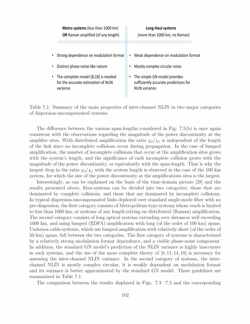
OR Raman amplified (of any length) (more than 1000 km, no Raman)

• Weak dependence on modulation format

• Mostly complex circular noise

• The simple GN model provides

sufficiently accurate predictions for

NLIN variance

• Strong dependence on modulation format

• Distinct phase-noise-like nature

• The complete model [8,18] is needed

for the accurate estimation of NLIN

variance

Metro systems (less than 1000 km) Long-Haul systems

NLIN in two major categories

Table 7.1: Summary of the main properties of inter-channel NLIN in two major categoriesof dispersion-uncompensated systems

The difference between the various span-lengths considered in Fig. 7.5(b) is once againconsistent with the observations regarding the magnitude of the power discontinuity at theamplifier sites. With distributed amplification the ratio χ2/χ1 is independent of the lengthof the link since no incomplete collisions occur during propagation. In the case of lumpedamplification, the number of incomplete collisions that occur at the amplification sites growswith the system’s length, and the significance of each incomplete collision grows with themagnitude of the power discontinuity, or equivalently with the span-length. That is why thelargest drop in the ratio χ2/χ1 with the system length is observed in the case of the 100 kmsystem, for which the size of the power discontinuity at the amplifications sites is the largest.

Interestingly, as can be explained on the basis of the time-domain picture [28] and theresults presented above, fiber-systems can be divided into two categories; those that aredominated by complete collisions, and those that are dominated by incomplete collisions.In typical dispersion-uncompensated links deployed over standard single-mode fiber with nopre-dispersion, the first category consists of Metropolitan-type systems whose reach is limitedto less than 1000 km, or systems of any length relying on distributed (Raman) amplification.The second category consists of long optical systems extending over distances well exceeding1000 km, and using lumped (EDFA) amplification with long (of the order of 100 km) spans.Undersea cable-systems, which use lumped amplification with relatively short (of the order of50 km) spans, fall between the two categories. The first category of systems is characterizedby a relatively strong modulation format dependence, and a visible phase-noise component.In addition, the standard GN model’s prediction of the NLIN variance is highly inaccuratein such systems, and the use of the more complete theory of [8, 11, 14, 18] is necessary forassessing the inter-channel NLIN variance. In the second category of systems, the inter-channel NLIN is mostly complex circular, it is weakly dependent on modulation formatand its variance is better approximated by the standard GN model. These guidelines aresummarized in Table 7.1.

The comparison between the results displayed in Figs. 7.3 –7.5 and the corresponding

102

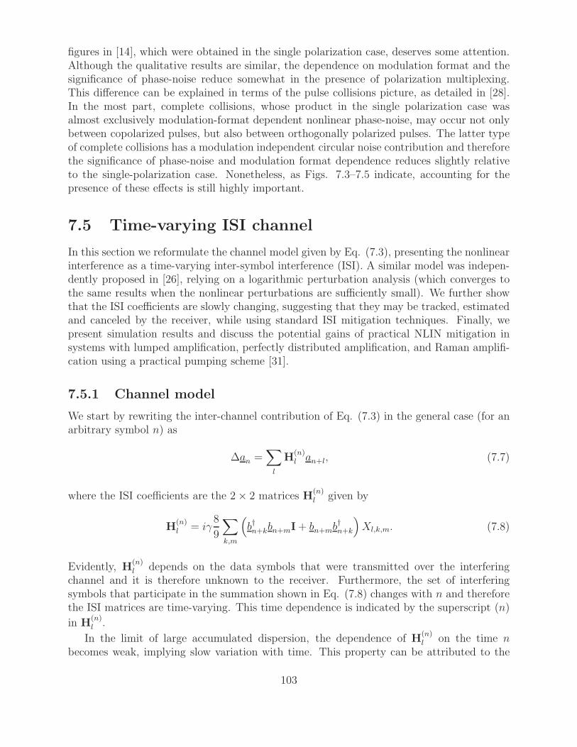
figures in [14], which were obtained in the single polarization case, deserves some attention.Although the qualitative results are similar, the dependence on modulation format and thesignificance of phase-noise reduce somewhat in the presence of polarization multiplexing.This difference can be explained in terms of the pulse collisions picture, as detailed in [28].In the most part, complete collisions, whose product in the single polarization case wasalmost exclusively modulation-format dependent nonlinear phase-noise, may occur not onlybetween copolarized pulses, but also between orthogonally polarized pulses. The latter typeof complete collisions has a modulation independent circular noise contribution and thereforethe significance of phase-noise and modulation format dependence reduces slightly relativeto the single-polarization case. Nonetheless, as Figs. 7.3–7.5 indicate, accounting for thepresence of these effects is still highly important.

7.5 Time-varying ISI channel

In this section we reformulate the channel model given by Eq. (7.3), presenting the nonlinearinterference as a time-varying inter-symbol interference (ISI). A similar model was indepen-dently proposed in [26], relying on a logarithmic perturbation analysis (which converges tothe same results when the nonlinear perturbations are sufficiently small). We further showthat the ISI coefficients are slowly changing, suggesting that they may be tracked, estimatedand canceled by the receiver, while using standard ISI mitigation techniques. Finally, wepresent simulation results and discuss the potential gains of practical NLIN mitigation insystems with lumped amplification, perfectly distributed amplification, and Raman amplifi-cation using a practical pumping scheme [31].

7.5.1 Channel model

We start by rewriting the inter-channel contribution of Eq. (7.3) in the general case (for anarbitrary symbol n) as

∆an =∑

l

H(n)l an+l, (7.7)

where the ISI coefficients are the 2× 2 matrices H(n)l given by

H(n)l = iγ

8

9

∑

k,m

(b†n+kbn+mI+ bn+mb

†n+k

)Xl,k,m. (7.8)

Evidently, H(n)l depends on the data symbols that were transmitted over the interfering

channel and it is therefore unknown to the receiver. Furthermore, the set of interferingsymbols that participate in the summation shown in Eq. (7.8) changes with n and thereforethe ISI matrices are time-varying. This time dependence is indicated by the superscript (n)

in H(n)l .

In the limit of large accumulated dispersion, the dependence of H(n)l on the time n

becomes weak, implying slow variation with time. This property can be attributed to the

103

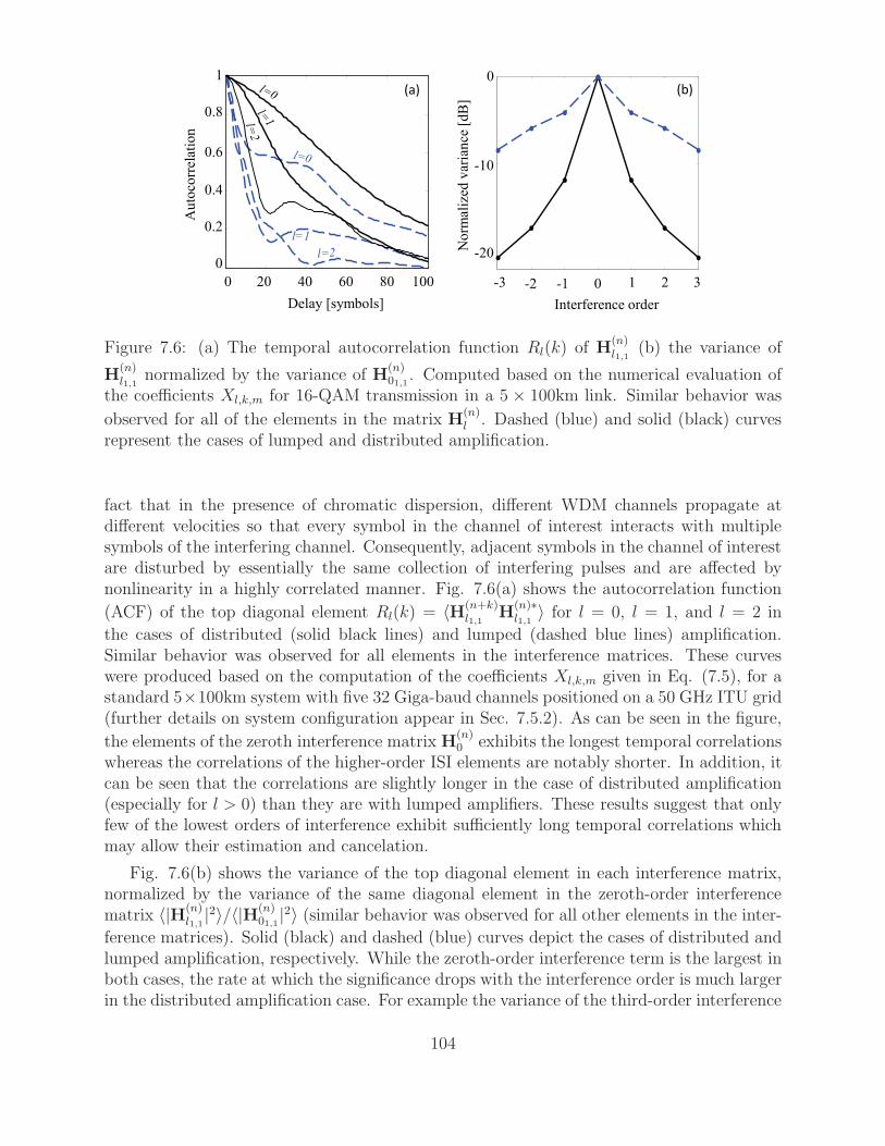
0

Delay [symbols]

20 40 60 80 100

0

0.2

0.4

0.6

0.8

1

Au

toco

rrel

atio

n

l=1

3- 1 2 32- 1- 0

20-

10-

0

Interference order

No

rmal

ized

var

ian

ce [

dB

]

(b)(a)

Figure 7.6: (a) The temporal autocorrelation function Rl(k) of H(n)l1,1

(b) the variance of

H(n)l1,1

normalized by the variance of H(n)01,1 . Computed based on the numerical evaluation of

the coefficients Xl,k,m for 16-QAM transmission in a 5 × 100km link. Similar behavior was

observed for all of the elements in the matrix H(n)l . Dashed (blue) and solid (black) curves

represent the cases of lumped and distributed amplification.

fact that in the presence of chromatic dispersion, different WDM channels propagate atdifferent velocities so that every symbol in the channel of interest interacts with multiplesymbols of the interfering channel. Consequently, adjacent symbols in the channel of interestare disturbed by essentially the same collection of interfering pulses and are affected bynonlinearity in a highly correlated manner. Fig. 7.6(a) shows the autocorrelation function

(ACF) of the top diagonal element Rl(k) = 〈H(n+k)l1,1

H(n)∗l1,1

〉 for l = 0, l = 1, and l = 2 in

the cases of distributed (solid black lines) and lumped (dashed blue lines) amplification.Similar behavior was observed for all elements in the interference matrices. These curveswere produced based on the computation of the coefficients Xl,k,m given in Eq. (7.5), for astandard 5×100km system with five 32 Giga-baud channels positioned on a 50 GHz ITU grid(further details on system configuration appear in Sec. 7.5.2). As can be seen in the figure,

the elements of the zeroth interference matrix H(n)0 exhibits the longest temporal correlations

whereas the correlations of the higher-order ISI elements are notably shorter. In addition, itcan be seen that the correlations are slightly longer in the case of distributed amplification(especially for l > 0) than they are with lumped amplifiers. These results suggest that onlyfew of the lowest orders of interference exhibit sufficiently long temporal correlations whichmay allow their estimation and cancelation.

Fig. 7.6(b) shows the variance of the top diagonal element in each interference matrix,normalized by the variance of the same diagonal element in the zeroth-order interferencematrix 〈|H(n)

l1,1|2〉/〈|H(n)

01,1|2〉 (similar behavior was observed for all other elements in the inter-

ference matrices). Solid (black) and dashed (blue) curves depict the cases of distributed andlumped amplification, respectively. While the zeroth-order interference term is the largest inboth cases, the rate at which the significance drops with the interference order is much largerin the distributed amplification case. For example the variance of the third-order interference

104

is smaller than the zeroth-order interference by ∼ 20dB in the distributed amplification casewhereas it is smaller by only ∼ 10dB in the case of lumped amplification. This implies thatthe benefit of canceling only the zeroth order would be much greater with distributed ampli-fication than it would be when lumped amplification is used. The fact that the dominance ofthe zeroth interference term is larger in the distributed amplification case is consistent withthe observations made in the previous section regarding the larger significance of phase-noisein this situation. This is because, as we discussed in Sec. 7.3, the diagonal terms H

(n)01,1

and

H(n)02,2 can be identified as contributing to phase-noise.

In what follows we present simulation results of practical NLIN mitigation, employingstandard ISI estimation, tracking and cancelation techniques, focusing exclusively on thecancelation of the zeroth order matrix H

(n)0 as it has the strongest impact and it exhibits

the longest temporal correlations. Attempts to compensate for higher ISI orders producednegligible benefits in the lumped amplification case. Since the potential gain in systems withdistributed amplification is much larger than it is in systems with lumped amplification,a practical compromise on which we test the performance of our mitigation, is a standardRaman amplified system, with parameters taken from [31]. As we show in what follows,the performance improvement extracted from NLIN mitigation in this case is quite notable.We further note that while the cancelation of the diagonal elements in the zeroth-orderinterference matrix H

(n)0 amounts to canceling the phase-noise part of the NLIN, cancelation

of the off-diagonal elements amounts to canceling circular NLIN originating from the lowestorder cross-polarization interference.

7.5.2 NLIN mitigation - simulation results

We have performed a series of simulations assuming a five-channel polarization multiplexedWDM system implemented over standard single-mode fiber (dispersion of 17 ps/nm/km,nonlinear coefficient γ = 1.3 [Wkm]−1, and attenuation of 0.2dB per km). The transmissionconsisted of Nyquist pulses at 32 Giga-baud and a standard channel spacing of 50 GHz. Themodulation format used by all WDM channels was 16-QAM where the number of simulatedsymbols in each run and for each polarization was 4096 when simulating a 500 km system, and8192 when simulating 6000 km. More than 100 runs (each with independent and random datasymbols) were performed with each set of system parameters, so as to accumulate sufficientstatistics. In the Raman amplified cases, a combination of co-propagating and counter-propagating Raman pumps was assumed, providing gains of 5 dB and 15 dB, respectively(as was done in [31]). At the receiver, the channel of interest was isolated with a matchedoptical filter and (perfectly, using 16 samples per symbol) back-propagated so as to eliminatethe effects of self-phase-modulation and chromatic dispersion. The noise figure of the lumpedamplifiers was 4dB and the Raman noise was generated with nsp = 1.26 (corresponding toa local NF of 4dB). In order to concentrate on the nonlinear noise mitigation aspects, weassumed ideal carrier phase and frequency estimation. To cancel the effect of the interferencematrix H

(n)0 we trained and tracked a canceling matrix, using a standard decision-aided

approach based on the recursive least squares (RLS) algorithm [32]. The RLS algorithmconverged faster than the more familiar least mean-squares (LMS) algorithm, and with asmall filter order, the added complexity is expected to be tolerable in future DSP used in

105

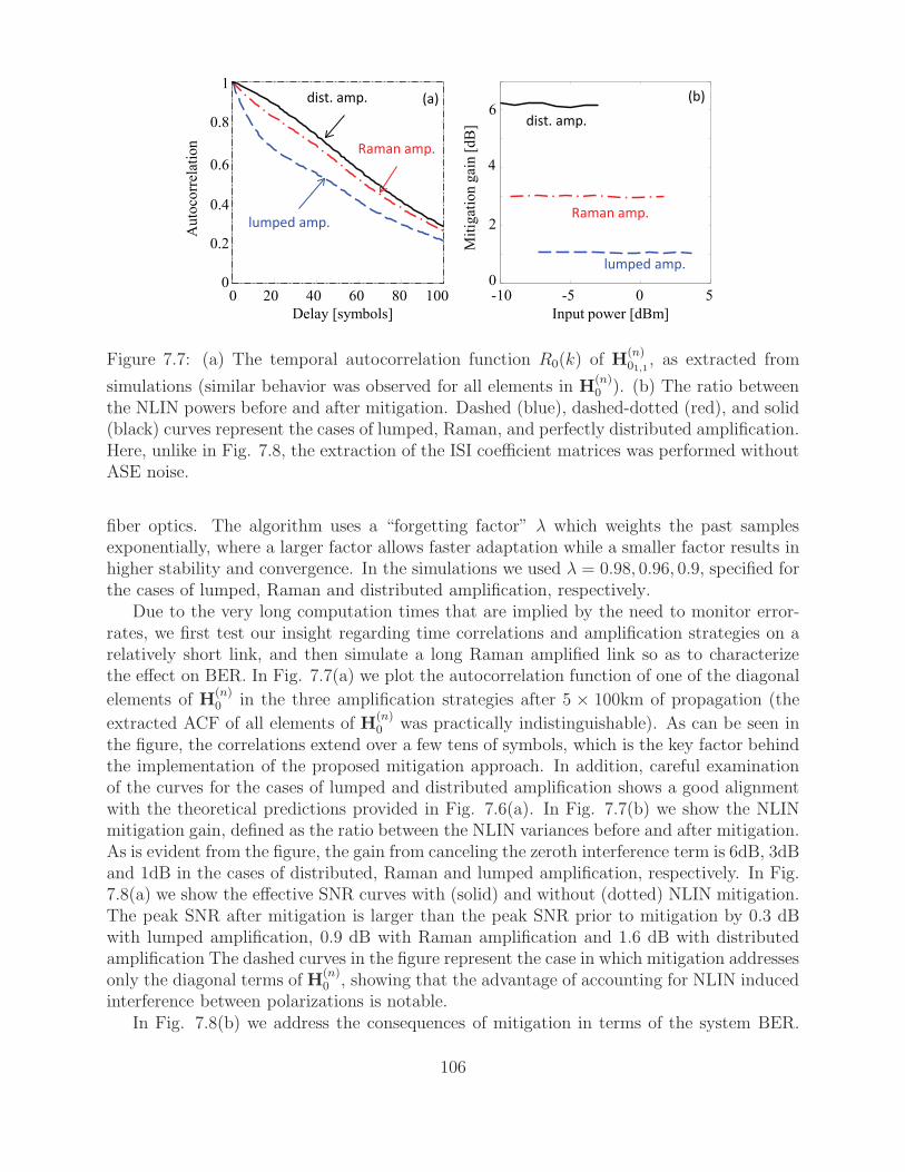
0

Delay [symbols]

20 40 60 80 1000

0.2

0.4

0.6

0.8

1(a)

Au

toco

rrel

atio

n

lumped amp.

Raman amp.

dist. amp. (b)

10-

Input power [dBm]

Mit

igat

ion

gai

n [

dB

]

5- 0 50

2

4

6

Raman amp.

dist. amp.

lumped amp.

(b)

Figure 7.7: (a) The temporal autocorrelation function R0(k) of H(n)01,1

, as extracted from

simulations (similar behavior was observed for all elements in H(n)0 ). (b) The ratio between

the NLIN powers before and after mitigation. Dashed (blue), dashed-dotted (red), and solid(black) curves represent the cases of lumped, Raman, and perfectly distributed amplification.Here, unlike in Fig. 7.8, the extraction of the ISI coefficient matrices was performed withoutASE noise.

fiber optics. The algorithm uses a “forgetting factor” λ which weights the past samplesexponentially, where a larger factor allows faster adaptation while a smaller factor results inhigher stability and convergence. In the simulations we used λ = 0.98, 0.96, 0.9, specified forthe cases of lumped, Raman and distributed amplification, respectively.

Due to the very long computation times that are implied by the need to monitor error-rates, we first test our insight regarding time correlations and amplification strategies on arelatively short link, and then simulate a long Raman amplified link so as to characterizethe effect on BER. In Fig. 7.7(a) we plot the autocorrelation function of one of the diagonal

elements of H(n)0 in the three amplification strategies after 5 × 100km of propagation (the

extracted ACF of all elements of H(n)0 was practically indistinguishable). As can be seen in

the figure, the correlations extend over a few tens of symbols, which is the key factor behindthe implementation of the proposed mitigation approach. In addition, careful examinationof the curves for the cases of lumped and distributed amplification shows a good alignmentwith the theoretical predictions provided in Fig. 7.6(a). In Fig. 7.7(b) we show the NLINmitigation gain, defined as the ratio between the NLIN variances before and after mitigation.As is evident from the figure, the gain from canceling the zeroth interference term is 6dB, 3dBand 1dB in the cases of distributed, Raman and lumped amplification, respectively. In Fig.7.8(a) we show the effective SNR curves with (solid) and without (dotted) NLIN mitigation.The peak SNR after mitigation is larger than the peak SNR prior to mitigation by 0.3 dBwith lumped amplification, 0.9 dB with Raman amplification and 1.6 dB with distributedamplification The dashed curves in the figure represent the case in which mitigation addressesonly the diagonal terms of H

(n)0 , showing that the advantage of accounting for NLIN induced

interference between polarizations is notable.In Fig. 7.8(b) we address the consequences of mitigation in terms of the system BER.

106

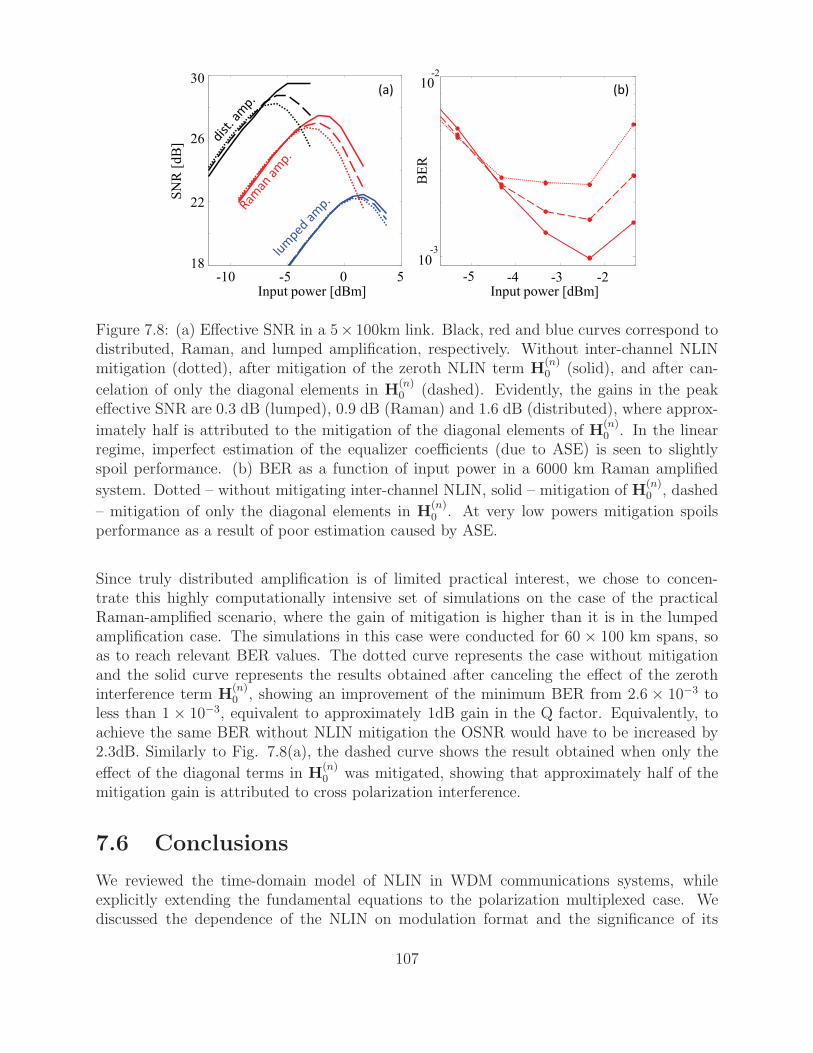
10-Input power [dBm]

SN

R[d

B]

5- 0 518

22

26

30

-5

10-3

Input power [dBm]

BE

R

-4 -3 -2

10-2

(a) (b)

Figure 7.8: (a) Effective SNR in a 5× 100km link. Black, red and blue curves correspond todistributed, Raman, and lumped amplification, respectively. Without inter-channel NLINmitigation (dotted), after mitigation of the zeroth NLIN term H

(n)0 (solid), and after can-

celation of only the diagonal elements in H(n)0 (dashed). Evidently, the gains in the peak

effective SNR are 0.3 dB (lumped), 0.9 dB (Raman) and 1.6 dB (distributed), where approx-

imately half is attributed to the mitigation of the diagonal elements of H(n)0 . In the linear

regime, imperfect estimation of the equalizer coefficients (due to ASE) is seen to slightlyspoil performance. (b) BER as a function of input power in a 6000 km Raman amplified

system. Dotted – without mitigating inter-channel NLIN, solid – mitigation of H(n)0 , dashed

– mitigation of only the diagonal elements in H(n)0 . At very low powers mitigation spoils

performance as a result of poor estimation caused by ASE.

Since truly distributed amplification is of limited practical interest, we chose to concen-trate this highly computationally intensive set of simulations on the case of the practicalRaman-amplified scenario, where the gain of mitigation is higher than it is in the lumpedamplification case. The simulations in this case were conducted for 60 × 100 km spans, soas to reach relevant BER values. The dotted curve represents the case without mitigationand the solid curve represents the results obtained after canceling the effect of the zerothinterference term H

(n)0 , showing an improvement of the minimum BER from 2.6 × 10−3 to

less than 1 × 10−3, equivalent to approximately 1dB gain in the Q factor. Equivalently, toachieve the same BER without NLIN mitigation the OSNR would have to be increased by2.3dB. Similarly to Fig. 7.8(a), the dashed curve shows the result obtained when only the

effect of the diagonal terms in H(n)0 was mitigated, showing that approximately half of the

mitigation gain is attributed to cross polarization interference.

7.6 Conclusions

We reviewed the time-domain model of NLIN in WDM communications systems, whileexplicitly extending the fundamental equations to the polarization multiplexed case. Wediscussed the dependence of the NLIN on modulation format and the significance of its

107

phase-noise component, as well as the accuracy and range of validity of the various models forpredicting the variance of NLIN. We showed that both the dependence on modulation formatand the phase-noise nature of inter-channel NLIN are particularly important in metro-lengthsystems, or in systems of any reach that use short spans, or Raman amplification. In thecase of long-haul systems (well over 1000 km) operating with long spans and using lumped(EDFA) amplification the significance of these phenomena is considerably smaller. Theobserved phenomena were related to the pulse collisions picture, whose details are providedseparately [28]. Finally, we introduced the slowly varying ISI model for the nonlinear channeland examined the improvement that can be achieved in system performance when mitigatinginter-channel NLIN by means of adaptive linear equalization (without joint processing ofmultiple WDM channels). We note that the proposed mitigation scheme has the advantageof using the same type of hardware currently used for equalizing polarization effects, yet theequalization algorithm and the required speed of convergence are substantially different.

Acknowledgement

The authors would like to acknowledge financial support from the Israel Science Foundation(grant 737/12). Ronen Dar would like to acknowledge the support of the Adams Fellowship ofthe Israel Academy of Sciences and Humanities, the Yitzhak and Chaya Weinstein ResearchInstitute, the Advanced Communication Center and the Electro-Optic Fund of Tel-AvivUniversity, and the Terasanta consortium.

7.7 Appendix: Time and frequency-domain represen-

tations of χ1 and χ2

The process of evaluating the variance of the NLIN involves the calculation of the secondmoment 〈∆a†∆a〉 from the (inter-channel) summation appearing in Eq. (7.3). The ideais that the FON coefficient χ2 can be found by identifying all terms in the second sum inEq. (7.3) that contribute to the existence of a fourth moment 〈|b|4〉. Then, the term χ1

is found such that the terms proportional to the second moment 〈|b|2〉2 are accounted for,in accordance with the form of Eq. (7.6). A cumbersome, yet straightforward calculation,produces the results

χ1 =32

27γ2∑

l,k,m

|Xl,k,m|2 (7.9)

χ2 =80

81γ2∑

l,m

|Xl,m,m|2 , (7.10)

where the nonlinear coefficients Xl,k,m are given in Eq. (7.5).

The frequency-domain representations of χ1 and χ2 can now be easily derived from thetime-domain representations given in Eqs. (7.9–7.10). Using the fact that g(L, t) is equalto∫g(ω) exp(−iωt+ iβ ′′ω2L/2)dω/(2π), where g(ω) is the inverse Fourier transform of the

108

fundamental pulse g(t), the expression for Xl,k,m can be rewritten as follows

Xl,k,m=

∫ρ(ω1, ω2, ω3)e

i(ω1l−ω2k+ω3m)T d3ω

(2π)3, (7.11)

where dnω stands for dω1 · · ·dωn and where

ρ(ω1, ω2, ω3)= g∗(ω1 − ω2 + ω3)g(ω1)g

∗(ω2 − Ω)g(ω3 − Ω)

×∫ L

0

f(z)eiβ′′(ω2−ω3)(ω2−ω1)zdz. (7.12)

Note that within the time-domain picture, the various contributions to NLIN are propor-tional to Xl,k,m, whereas the frequency-domain representation consists of the contributionsof multiple FWM products that are proportional to ρ(ω1, ω2, ω3) (each contribution is pro-duced by FWM between the frequency tone at ω1 in the channel of interest and the frequencytones at ω2 and ω3 in the interfering channel). Equation (7.11) reveals an interesting relationbetween the time-domain and frequency-domain analyses where Xl,k,m and ρ(ω1, ω2, ω3) arerelated through the 3-dimensional Fourier transform.

Substitution of Eq. (7.11) into Eq. (7.9) results in

χ1=32

27γ2∑

l,k,m

∫ei(ω1−ω′

1)lT e−i(ω2−ω′2)kT ei(ω3−ω′

3)mT

×ρ(ω1, ω2, ω3)ρ∗(ω′

1, ω′2, ω

′3)

d3ω

(2π)3d3ω′

(2π)3, (7.13)

where for simplicity we assumed perfect Nyquist pulses so that g(ω)g(ω ± 2π/T ) = 0. Inthis case, by using the identity

∞∑

k=−∞eikTω =

2π

T

∞∑

n=−∞δ

(ω − 2πn

T

)(7.14)

we find that

χ1=32

27

γ2

T 3

∫|ρ(ω1, ω2, ω3)|2

d3ω

(2π)3. (7.15)

In the same manner it can be shown that χ2 is equal to

χ2=80

81

γ2

T 2

∫ρ(ω1, ω2, ω3)ρ

∗(ω1, ω4, ω4+ω3−ω2)d4ω

(2π)4. (7.16)

The SON and FON coefficients χ1 and χ2 can be therefore calculated by computing a threeand four dimension integrals, respectively. Such integration is readily performed using theMonte Carlo integration method [33], whose implementation is described in the appendixof [14].

109

Bibliography

[1] R.-J. Essiambre, G. Kramer, P.J. Winzer, G.J. Foschini, B. Goebel, “Capacity limits ofoptical fiber networks,” J. Lightwave Technol., vol. 28, pp. 662–701 (2010).

[2] A. D. Ellis, J. Zhao, D. Cotter, “Approaching the non-linear Shannon limit,” J. Light-wave Technol., vol 28, pp. 423–433 (2010).

[3] A. Mecozzi, C. B. Clausen, and M. Shtaif, “Analysis of intrachannel nonlinear effects inhighly dispersed optical pulse transmission,” IEEE Photon. Technol. Lett., vol 12, pp.392-394 (2000).

[4] F. Forghieri, R.W. Tkack, A. R. Chraplyvy, “Fiber nonlinearities and their impact ontransmission systems,” Ch. 8 in Optical Fiber Telecommunications IIIA, P. Kaminowand T. L. Koch eds. (Academic Press, 1997).

[5] E. Ip, J. M. Kahn, “Compensation of dispersion and nonlinear impairments using digitalbackpropagation,” J. Lightwave Technol., vol. 26, pp. 3416-3425 (2008).

[6] R. I. Killey, P. M. Watts, V. Mikhailov, M. Glick, P. Bayvel, “Electronic dispersioncompensation by signal predistortion using digital processing and a dual-drive Mach-Zehnder modulator,” IEEE Photon. Technol. Lett., vol 17, pp. 714-716 (2005).

[7] E. Ip, “Nonlinear compensation using backpropagation for polarization-multiplexedtransmission,” J. Lightwave Technol., vol 28, pp. 939–951 (2010).

[8] R. Dar, M. Feder, A. Mecozzi, M. Shtaif, “Properties of nonlinear noise in long,dispersion-uncompensated fiber links,” Optics Express, vol. 21, pp. 25685–25699 (2013).

[9] A. Carena, V. Curri, G. Bosco, P. Poggiolini, F. Forghieri, “Modeling of the impact ofnonlinear propagation effects in uncompensated optical coherent transmission links,” J.Lightwave Technol., vol. 30, pp. 1524–1539 (2012).

[10] A. Bononi, N. Rossi, P. Serena, “On the nonlinear threshold versus distance in long-haulhighly-dispersive coherent systems,” Optics Express, vol. 20, pp. B204–B216 (2012).

[11] R. Dar, M. Feder, A. Mecozzi, M. Shtaif, Nonlinear interference noise wizard. Availableat: http://nlinwizard.eng.tau.ac.il

[12] P. Poggiolini, G. Bosco, A. Carena, V. Curri, Y. Jiang, F. Forghieri, “The GN-modelof fiber non-linear propagation and its applications,” J. Lightwave Technol., vol. 4, pp.100–127 (2014).

110

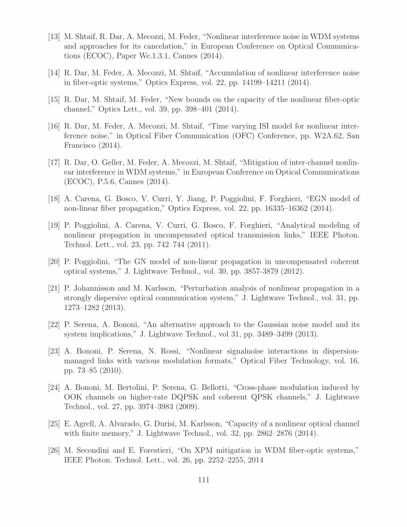
[13] M. Shtaif, R. Dar, A. Mecozzi, M. Feder, “Nonlinear interference noise in WDM systemsand approaches for its cancelation,” in European Conference on Optical Communica-tions (ECOC), Paper We.1.3.1, Cannes (2014).

[14] R. Dar, M. Feder, A. Mecozzi, M. Shtaif, “Accumulation of nonlinear interference noisein fiber-optic systems,” Optics Express, vol. 22, pp. 14199–14211 (2014).

[15] R. Dar, M. Shtaif, M. Feder, “New bounds on the capacity of the nonlinear fiber-opticchannel,” Optics Lett., vol. 39, pp. 398–401 (2014).

[16] R. Dar, M. Feder, A. Mecozzi, M. Shtaif, “Time varying ISI model for nonlinear inter-ference noise,” in Optical Fiber Communication (OFC) Conference, pp. W2A.62, SanFrancisco (2014).

[17] R. Dar, O. Geller, M. Feder, A. Mecozzi, M. Shtaif, “Mitigation of inter-channel nonlin-ear interference in WDM systems,” in European Conference on Optical Communications(ECOC), P.5.6, Cannes (2014).

[18] A. Carena, G. Bosco, V. Curri, Y. Jiang, P. Poggiolini, F. Forghieri, “EGN model ofnon-linear fiber propagation,” Optics Express, vol. 22, pp. 16335–16362 (2014).

[19] P. Poggiolini, A. Carena, V. Curri, G. Bosco, F. Forghieri, “Analytical modeling ofnonlinear propagation in uncompensated optical transmission links,” IEEE Photon.Technol. Lett., vol. 23, pp. 742–744 (2011).

[20] P. Poggiolini, “The GN model of non-linear propagation in uncompensated coherentoptical systems,” J. Lightwave Technol., vol. 30, pp. 3857-3879 (2012).

[21] P. Johannisson and M. Karlsson, “Perturbation analysis of nonlinear propagation in astrongly dispersive optical communication system,” J. Lightwave Technol., vol. 31, pp.1273–1282 (2013).

[22] P. Serena, A. Bononi, “An alternative approach to the Gaussian noise model and itssystem implications,” J. Lightwave Technol., vol 31, pp. 3489–3499 (2013).

[23] A. Bononi, P. Serena, N. Rossi, “Nonlinear signalnoise interactions in dispersion-managed links with various modulation formats,” Optical Fiber Technology, vol. 16,pp. 73–85 (2010).

[24] A. Bononi, M. Bertolini, P. Serena, G. Bellotti, “Cross-phase modulation induced byOOK channels on higher-rate DQPSK and coherent QPSK channels,” J. LightwaveTechnol., vol. 27, pp. 3974–3983 (2009).

[25] E. Agrell, A. Alvarado, G. Durisi, M. Karlsson, “Capacity of a nonlinear optical channelwith finite memory,” J. Lightwave Technol., vol. 32, pp. 2862–2876 (2014).

[26] M. Secondini and E. Forestieri, “On XPM mitigation in WDM fiber-optic systems,”IEEE Photon. Technol. Lett., vol. 26, pp. 2252–2255, 2014

111

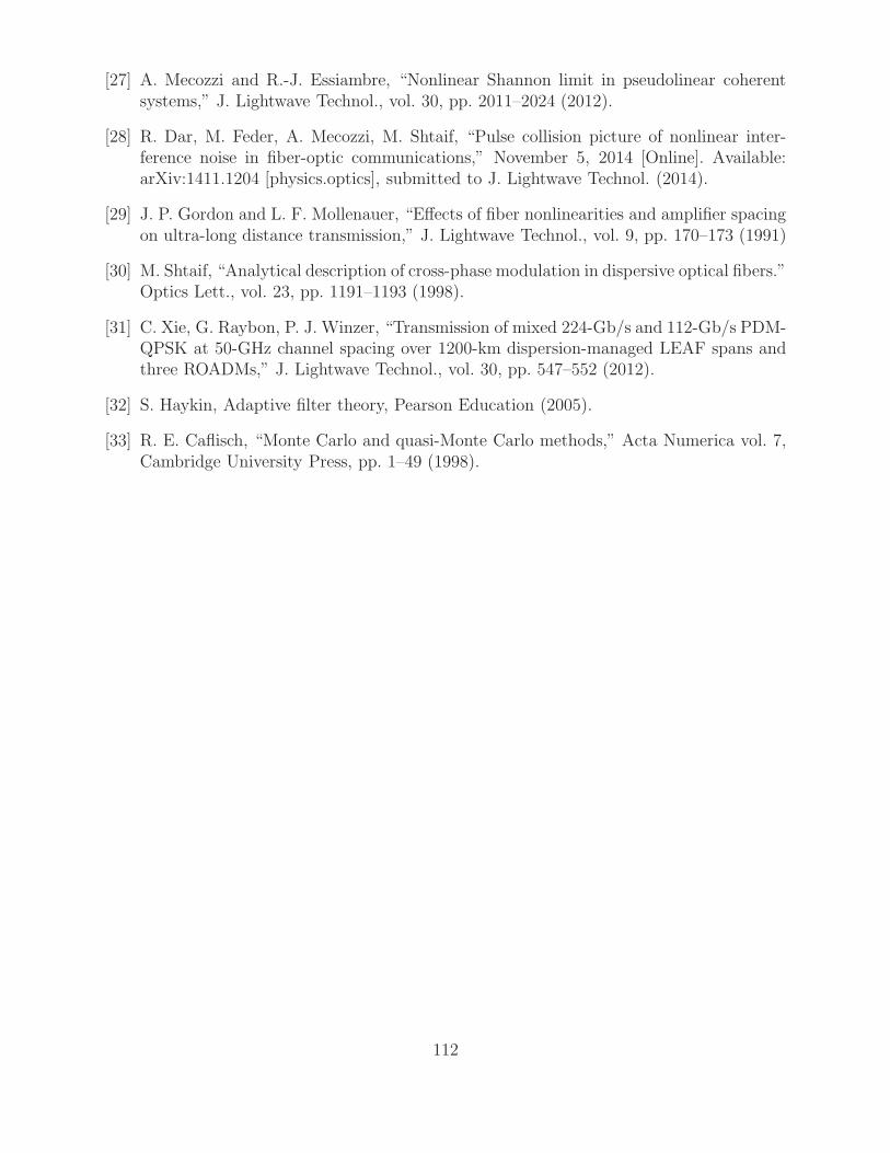
[27] A. Mecozzi and R.-J. Essiambre, “Nonlinear Shannon limit in pseudolinear coherentsystems,” J. Lightwave Technol., vol. 30, pp. 2011–2024 (2012).

[28] R. Dar, M. Feder, A. Mecozzi, M. Shtaif, “Pulse collision picture of nonlinear inter-ference noise in fiber-optic communications,” November 5, 2014 [Online]. Available:arXiv:1411.1204 [physics.optics], submitted to J. Lightwave Technol. (2014).

[29] J. P. Gordon and L. F. Mollenauer, “Effects of fiber nonlinearities and amplifier spacingon ultra-long distance transmission,” J. Lightwave Technol., vol. 9, pp. 170–173 (1991)

[30] M. Shtaif, “Analytical description of cross-phase modulation in dispersive optical fibers.”Optics Lett., vol. 23, pp. 1191–1193 (1998).

[31] C. Xie, G. Raybon, P. J. Winzer, “Transmission of mixed 224-Gb/s and 112-Gb/s PDM-QPSK at 50-GHz channel spacing over 1200-km dispersion-managed LEAF spans andthree ROADMs,” J. Lightwave Technol., vol. 30, pp. 547–552 (2012).

[32] S. Haykin, Adaptive filter theory, Pearson Education (2005).

[33] R. E. Caflisch, “Monte Carlo and quasi-Monte Carlo methods,” Acta Numerica vol. 7,Cambridge University Press, pp. 1–49 (1998).

112

Chapter 8

Pulse Collision Picture of

Inter-Channel Nonlinear Interference


Ronen Dar, Meir Feder, Antonio Mecozzi and Mark Shtaif, “Pulse collision picture of inter-channel nonlinear interference in fiber-optic communications,” accepted for publication inIEEE Journal of Lightwave Technology (April 2015)

8.1 Abstract

We model the build-up of inter-channel nonlinear interference noise (NLIN) in wavelengthdivision multiplexed systems by considering the pulse collision dynamics in the time domain.The fundamental interactions can be classified as two-pulse, three-pulse, or four-pulse colli-sions and they can be either complete, or incomplete. Each type of collision is shown to haveits unique signature and the overall nature of NLIN is determined by the relative importanceof the various classes of pulse collisions in a given WDM system. The pulse-collision pictureprovides qualitative and quantitative insight into the character of NLIN, offering a simpleand intuitive explanation to all of the reported and previously unexplained phenomena. Inparticular, we show that the most important contributions to NLIN follow from two-pulseand four-pulse collisions. While the contribution of two-pulse collisions is in the form ofphase-noise and polarization-state-rotation with strong dependence on modulation format,four-pulse collisions generate complex circular noise whose variance is independent of modu-lation format. In addition, two-pulse collisions are strongest when the collision is complete,whereas four-pulse collisions are strongest when the collision is incomplete. We show thattwo-pulse collisions dominate the formation of NLIN in short links with lumped amplification,or in links with distributed amplification extending over arbitrary length. In long links usinglumped amplification the relative significance of four-pulse collisions increases, emphasizingthe circularity of the NLIN while reducing its dependence on modulation format.

113

8.2 Introduction

The nonlinearity of optical fibers has been long recognized as one of the most importantfactors limiting the growth of data-rates transmitted in wavelength division multiplexed(WDM) systems [1]. The nonlinear distortions are usually classified as either intra-channel[2], or inter-channel [3]. While intra-channel distortions are generated by each of the WDMchannels individually, inter-channel distortions are caused by interference between differentWDM channels. In this work we focus on the physical mechanism responsible for inter-channel nonlinear effects as it comes into play in modern, dispersion uncompensated fiberlinks with coherent detection. Since joint processing of multiple WDM channels is currentlyconsidered to be prohibitively complex in commercial systems, inter-channel interferenceis customarily treated as noise [1], and hence we refer to it in what follows as nonlinearinterference noise, or NLIN [4–9].

We follow up on the theory published in [4,6,10] and model in the time domain1 the build-up of NLIN in WDM systems which are using single-carrier transmission. In this approachinter-channel NLIN is attributed to multiple pulse collisions whose dynamics we examinein detail (a similar analysis of intra-channel pulse-interactions can be found in [2, 14]). Aswe demonstrate in what follows, the pulse-collision picture provides deep quantitative andqualitative insight into the build-up of NLIN, and explains the various properties of NLINthat have previously only been observed empirically in simulations. For example, issues likethe importance of the phase-noise component of the NLIN versus the legitimacy of describingNLIN as complex circular noise, the dependence of the NLIN power on modulation format,the effect of pre-dispersion, the dependence on system-length and type of amplification,etc. [4–6, 15–18], are all clarified once the essence of pulse collision dynamics is understood.

While the practice of analyzing nonlinear interference by means of pulse collisions hasbeen known for a while (initially in the context of soliton [19, 20] and dispersion-managed-soliton [21,22] transmission, and subsequently in the more general context of arbitrary pulseinteractions [23]), the pulse collision dynamics encountered in modern coherent fiber com-munications systems, has a number of fundamentally different characteristics. Most promi-nently, in modern systems, which avoid the use of inline dispersion compensation, simulta-neous multi-pulse collisions play a unique and very significant role. In order to illustratethis, consider the case where the channel of interest is perturbed by a nonlinear interactionwith a single interfering WDM channel. In the old generation of dispersion managed sys-tems [21–23], interference was generated by collisions between pairs of pulses, one from thechannel of interest and one from the interfering channel. In the new generation of dispersionuncompensated systems, pulse spreading generates significant temporal overlap within eachof the channels, allowing for example, situations in which two different pulses in the inter-fering channel interact nonlinearly with a third pulse, belonging to the channel of interest,so as to generate interference that affects a fourth pulse, also belonging to the channel ofinterest.

In what follows we demonstrate that substantial understanding of a broad range of ob-served nonlinear interference phenomena can be achieved by means of proper classificationof the type of collisions taking place in the fiber. Most relevantly, there is a qualitative and

1Other time-domain models for inter-channel effects were considered in [11–13]

114

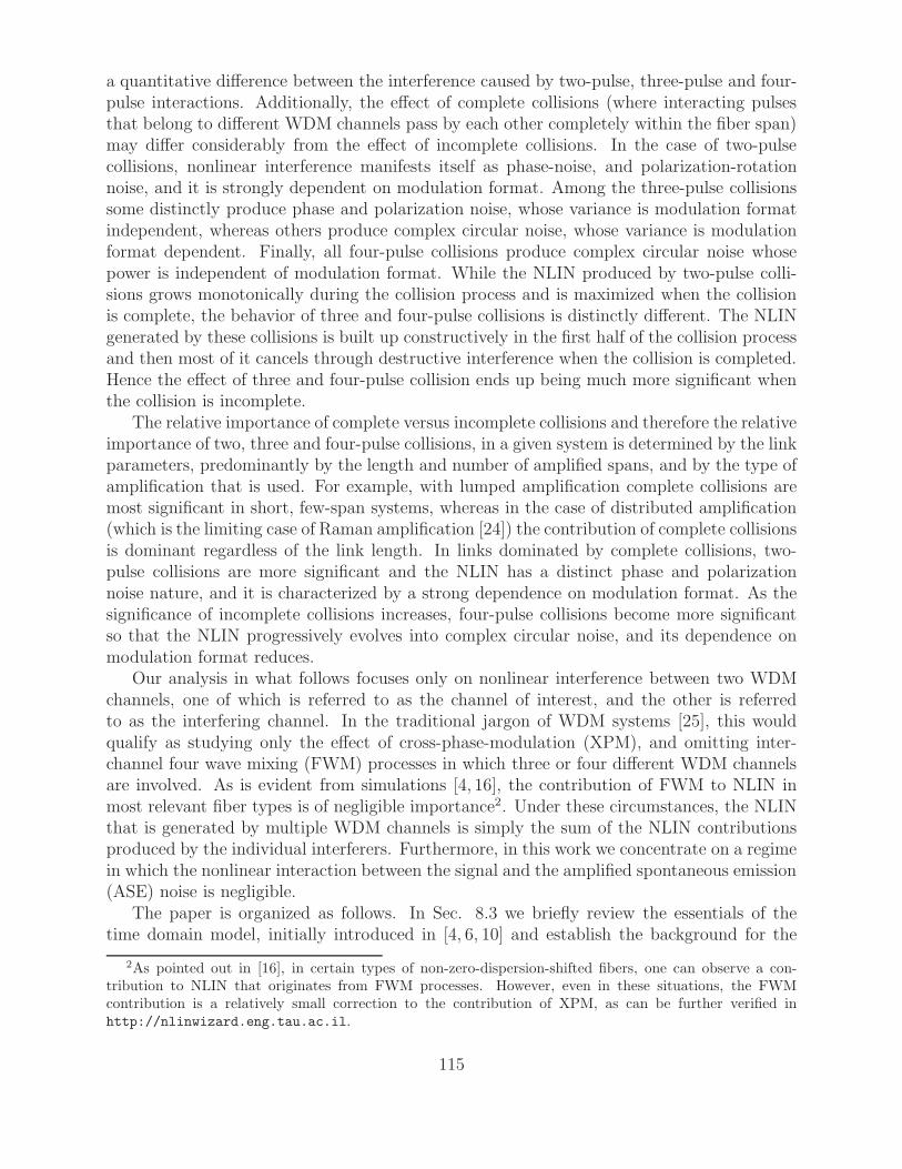
a quantitative difference between the interference caused by two-pulse, three-pulse and four-pulse interactions. Additionally, the effect of complete collisions (where interacting pulsesthat belong to different WDM channels pass by each other completely within the fiber span)may differ considerably from the effect of incomplete collisions. In the case of two-pulsecollisions, nonlinear interference manifests itself as phase-noise, and polarization-rotationnoise, and it is strongly dependent on modulation format. Among the three-pulse collisionssome distinctly produce phase and polarization noise, whose variance is modulation formatindependent, whereas others produce complex circular noise, whose variance is modulationformat dependent. Finally, all four-pulse collisions produce complex circular noise whosepower is independent of modulation format. While the NLIN produced by two-pulse colli-sions grows monotonically during the collision process and is maximized when the collisionis complete, the behavior of three and four-pulse collisions is distinctly different. The NLINgenerated by these collisions is built up constructively in the first half of the collision processand then most of it cancels through destructive interference when the collision is completed.Hence the effect of three and four-pulse collision ends up being much more significant whenthe collision is incomplete.

The relative importance of complete versus incomplete collisions and therefore the relativeimportance of two, three and four-pulse collisions, in a given system is determined by the linkparameters, predominantly by the length and number of amplified spans, and by the type ofamplification that is used. For example, with lumped amplification complete collisions aremost significant in short, few-span systems, whereas in the case of distributed amplification(which is the limiting case of Raman amplification [24]) the contribution of complete collisionsis dominant regardless of the link length. In links dominated by complete collisions, two-pulse collisions are more significant and the NLIN has a distinct phase and polarizationnoise nature, and it is characterized by a strong dependence on modulation format. As thesignificance of incomplete collisions increases, four-pulse collisions become more significantso that the NLIN progressively evolves into complex circular noise, and its dependence onmodulation format reduces.

Our analysis in what follows focuses only on nonlinear interference between two WDMchannels, one of which is referred to as the channel of interest, and the other is referredto as the interfering channel. In the traditional jargon of WDM systems [25], this wouldqualify as studying only the effect of cross-phase-modulation (XPM), and omitting inter-channel four wave mixing (FWM) processes in which three or four different WDM channelsare involved. As is evident from simulations [4, 16], the contribution of FWM to NLIN inmost relevant fiber types is of negligible importance2. Under these circumstances, the NLINthat is generated by multiple WDM channels is simply the sum of the NLIN contributionsproduced by the individual interferers. Furthermore, in this work we concentrate on a regimein which the nonlinear interaction between the signal and the amplified spontaneous emission(ASE) noise is negligible.

The paper is organized as follows. In Sec. 8.3 we briefly review the essentials of thetime domain model, initially introduced in [4, 6, 10] and establish the background for the

2As pointed out in [16], in certain types of non-zero-dispersion-shifted fibers, one can observe a con-tribution to NLIN that originates from FWM processes. However, even in these situations, the FWMcontribution is a relatively small correction to the contribution of XPM, as can be further verified inhttp://nlinwizard.eng.tau.ac.il.

115

t

t

-th

pulse

zeroth

pulse

= 0 =

| |

m + /2

( )

-th

pulse-th

pulse

WDM channels

t

t

m + /2 z

WDM channels

Figure 8.1: The generic four-pulse interference. The h-th pulse in the channel of interestinteracts with the k-th and m-th pulses of the interfering channel so as to create NLIN thataffects the zeroth symbol in the channel of interest. Since we assume detection that involvesfiltering matched to the waveform of the fundamental pulse centered at the zeroth symbol,as discussed in Sec. 8.3, one can refer to this as a four-pulse interaction. The zeroth pulseis plotted only to keep track of the matched-filter waveform, and it is plotted by a dashedline in order to stress that it is not a pulse that is physically participating in the nonlinearinteraction during propagation. The left panel shows the situation in the beginning of thelink, before the pulses overlap, whereas the right panel illustrates the situation once anoverlap between the pulses is formed. When two of the indices overlap (h = 0, or k = m)one observes a three-pulse interaction and when both index pairs overlap (h = 0 and k = m)one obtains a two-pulse interaction.

subsequent analysis. In Secs. 8.4, 8.5, and 8.6 we classify the nonlinear interference pro-cesses as two, three and four-pulse collisions, respectively. In each case we describe theirdistinctive features depending on whether the collision is complete, or incomplete. Severalnumerical examples illustrating the main ideas are presented in Sec. 8.7. For the simplicityof illustration Secs. 8.3–8.6 consider scalar (single-polarization) transmission. The extensionto the polarization multiplexed case is presented in Sec. 8.8. In Sec. 8.9 we discuss theimplications of the pulse-collision theory to fiber-communications systems, whereas in Sec.8.10 we explain the role of chromatic dispersion and relate the time domain theory to theGaussian noise (GN) model [26–30]. Section 8.11 is devoted to conclusions.

8.3 Time-domain theory

For the simplicity of illustration we start by considering the single-polarization case, post-poning the generalization to polarization multiplexed systems to Sec. 8.8. In the case of twoWDM channels, we may express the electric field at the fiber input as

∑

n

ang(0, t− nT ) + exp(−iΩt)∑

n

bng(0, t− nT ), (8.1)

where T is the symbol duration and an and bn are the complex valued data symbols trans-mitted over the channel of interest and over the interfering channel, respectively. The central

116

frequency of the channel of interest is arbitrarily set to 0, whereas the central frequency ofthe interfering channel is denoted by Ω. The injected fundamental symbol waveforms inboth channels are identical and denoted by g(0, t), whereas g(z, t) = exp(− i

2β ′′z ∂2

∂t2)g(0, t) is

the dispersed waveform of the individual pulse when reaching point z along the fiber withβ ′′ being the fiber dispersion coefficient3. The fundamental waveforms are further assumedto be orthogonal with respect to time shifts by an integer number of symbol durations andtheir energy is assumed to be normalized to 1

∫g∗(z, t− nT )g(z, t− n′T )dt = δn,n′. (8.2)

After coherent detection, the channel of interest is match-filtered with the filter’s impulseresponse being proportional to g∗(L, t), where L is the link length. The extracted n-th datasymbol can be then expressed as an +∆an, with ∆an accounting for the presence of NLIN.In [4] we have shown that ∆an due to inter-channel NLIN is given by

∆a0=2iγ∑

h,k,m

ahb∗kbmXh,k,m. (8.3)

where γ is the nonlinear coefficient and where we have arbitrarily (and without loss ofgenerality) set the index of the received symbol to 0. The coefficients Xh,k,m have beenintroduced in Ref. [4], where they have been shown to be

Xh,k,m=

∫ L

0

dz f(z)

∫ ∞

−∞dt g∗(z, t)g(z, t− hT )

×g∗(z, t−kT−β ′′Ωz)g(z, t−mT−β ′′Ωz). (8.4)

The function f(z) accounts for the loss/gain profile along the link [4, 10]. For example,f(z) = 1 in the case of perfectly distributed amplification and f(z) = exp(−αmod(z, Ls))in the case of lumped amplification where α is the loss coefficient and Ls is the span length.

The coefficient Xh,k,m is associated with the NLIN that is observed in the measurement ofthe zeroth data symbol in the channel of interest following the nonlinear interaction betweenthe h-th pulse in the channel of interest and the k-th and m-th pulses in the interferingchannel, as illustrated in Fig. 8.1. The triple product ξ(z, t) = g(z, t − hT )g∗(z, t−kT−β ′′Ωz)g(z, t−mT−β ′′Ωz), appearing in the integrand of Eq. (8.4), describes a classic non-linear Kerr interaction taking place at time t and position z along the link (where β ′′Ω isthe difference between the reciprocal group velocities). This product then propagates to-wards the receiver, while accumulating the dispersion present in the remaining fiber-length,which is equal to L − z. Since the impulse response of the matched filter is proportionalto g∗(L, t) = exp( i

2β ′′(L − z) ∂2

∂t2)g∗(z, t), this accumulated dispersion is removed. The sam-

pled perturbation at the receiver, as the inner integral in Eq. (8.4) suggests, is therefore∫g∗(z, t)ξ(z, t)dt, which can be interpreted as if the nonlinear product ξ(z, t) was matched

filtered by a ‘fourth’ pulse g∗(z, t) exactly at the position along the link at which the Kerr in-teraction occurred. The integral over z in Eq. (8.4) gathers the nonlinear products producedalong the entire link.

3As we are relying on a first order perturbation analysis – the waveform g(z, t) includes only the effect ofdispersion and not the effect of nonlinearity. In [4] we used g(0)(z, t) for the same quantity.

117

We now proceed to classifying the various contributions to the NLIN in terms of the typeof collisions that produce them. In the most general case, these contributions are producedby nonlinear interactions between four pulses – the “dummy” zeroth pulse from the channelof interest (accounting for the fact that the signal is matched filtered at the receiver), theh-th pulse from the channel of interest, and the k-th and m-th pulses from the interferingchannel. When some of the indices coincide, as we shall see in the following sections, atwo-pulse, or three-pulse collision is formed.

8.4 Two-pulse collisions

A two-pulse collision occurs when one of the interacting pulses is the pulse of interest,which we arbitrarily select as the zeroth-index pulse, whereas the other pulse belongs to theinterfering channel, so that h = 0 and k = m. The strength of this interaction is governedby the coefficient

X0,m,m=

∫ L

0

dzf(z)

∫ ∞

−∞dt |g(z, t)|2 |g(z, t−mT−β ′′Ωz)|2, (8.5)

and, according to Eq. (8.3), it produces a perturbation equal to ia0(2γX0,m,m|bm|2). AsX0,m,m is a real-valued quantity the perturbation is at a complex angle of π/2 from thetransmitted symbol a0. Namely, the perturbation generated by two-pulse interactions hasthe character of phase-noise.

An interesting perspective into this reality can be obtained by considering the ‘old class’of two-pulse collisions initially studied in the context of solitons [19–22]. There, it hasbecome common knowledge that when a pulse in the channel of interest undergoes a completecollision with an interfering pulse belonging to an adjacent WDM channel, the only notableconsequence observed on the pulse of interest is a time-independent phase-shift. However, itis also well known that when the collision between the two pulses is not complete [22, 23],the phase of the interacting pulses is distorted via XPM leading to the formation of a time-dependent phase distortion (nonlinear chirp), which subsequently produces an amplitude (ortiming-jitter) perturbation after being affected by the dispersion of the remaining fiber. Notethat in the scheme that we consider here, no amplitude perturbation is formed in two-pulsecollisions, regardless of whether the collisions are complete, or incomplete. This differencewith respect to the old generation of systems can be attributed to coherent detection andthe use of a matched filter, which is equivalent to measuring the perturbation at the pointalong the fiber where the collision takes place, as explained earlier. Namely, the effect ofdispersion, which translates the time-dependent phase distortion into amplitude variationsis reversed by the matched filter.

Since in addition to being real-valued, the integrand in Eq. (8.5) is also non-negative,the nonlinear phase-shift is proportional to the “completeness” of the collision, namely thephase-shift is zero when the waveforms do not overlap at all during propagation and it ismaximized when the collision is complete. As we demonstrate in Appendix 8.12, two-pulsecollision coefficients X0,m,m scale as Ω−1. In addition, the fact that two-pulse contributions toNLIN are proportional to a0|bm|2 implies that the variance of NLIN that is associated withthese contributions is proportional to 〈|a0|2〉(〈|bm|4〉 − 〈|bm|2〉2), with the angled brackets

118

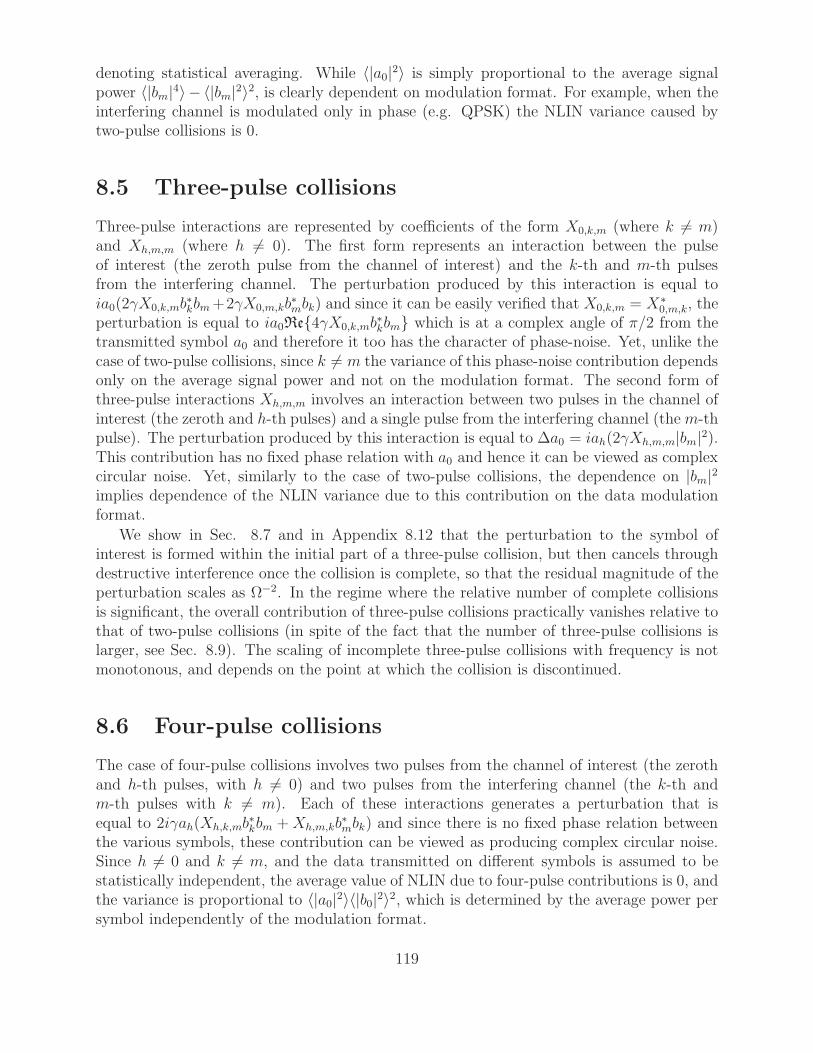
denoting statistical averaging. While 〈|a0|2〉 is simply proportional to the average signalpower 〈|bm|4〉 − 〈|bm|2〉2, is clearly dependent on modulation format. For example, when theinterfering channel is modulated only in phase (e.g. QPSK) the NLIN variance caused bytwo-pulse collisions is 0.

8.5 Three-pulse collisions

Three-pulse interactions are represented by coefficients of the form X0,k,m (where k 6= m)and Xh,m,m (where h 6= 0). The first form represents an interaction between the pulseof interest (the zeroth pulse from the channel of interest) and the k-th and m-th pulsesfrom the interfering channel. The perturbation produced by this interaction is equal toia0(2γX0,k,mb

∗kbm+2γX0,m,kb

∗mbk) and since it can be easily verified that X0,k,m = X∗

0,m,k, theperturbation is equal to ia0Re4γX0,k,mb

∗kbm which is at a complex angle of π/2 from the

transmitted symbol a0 and therefore it too has the character of phase-noise. Yet, unlike thecase of two-pulse collisions, since k 6= m the variance of this phase-noise contribution dependsonly on the average signal power and not on the modulation format. The second form ofthree-pulse interactions Xh,m,m involves an interaction between two pulses in the channel ofinterest (the zeroth and h-th pulses) and a single pulse from the interfering channel (them-thpulse). The perturbation produced by this interaction is equal to ∆a0 = iah(2γXh,m,m|bm|2).This contribution has no fixed phase relation with a0 and hence it can be viewed as complexcircular noise. Yet, similarly to the case of two-pulse collisions, the dependence on |bm|2implies dependence of the NLIN variance due to this contribution on the data modulationformat.

We show in Sec. 8.7 and in Appendix 8.12 that the perturbation to the symbol ofinterest is formed within the initial part of a three-pulse collision, but then cancels throughdestructive interference once the collision is complete, so that the residual magnitude of theperturbation scales as Ω−2. In the regime where the relative number of complete collisionsis significant, the overall contribution of three-pulse collisions practically vanishes relative tothat of two-pulse collisions (in spite of the fact that the number of three-pulse collisions islarger, see Sec. 8.9). The scaling of incomplete three-pulse collisions with frequency is notmonotonous, and depends on the point at which the collision is discontinued.

8.6 Four-pulse collisions

The case of four-pulse collisions involves two pulses from the channel of interest (the zerothand h-th pulses, with h 6= 0) and two pulses from the interfering channel (the k-th andm-th pulses with k 6= m). Each of these interactions generates a perturbation that isequal to 2iγah(Xh,k,mb

∗kbm +Xh,m,kb

∗mbk) and since there is no fixed phase relation between

the various symbols, these contribution can be viewed as producing complex circular noise.Since h 6= 0 and k 6= m, and the data transmitted on different symbols is assumed to bestatistically independent, the average value of NLIN due to four-pulse contributions is 0, andthe variance is proportional to 〈|a0|2〉〈|b0|2〉2, which is determined by the average power persymbol independently of the modulation format.

119

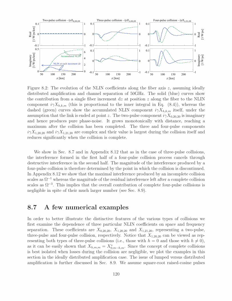
Imag

inar

y

[1/W

/ps/

km

]

Rea

l

[1/W

/ps/

km

]

Two-pulse collision - , , Three-pulse collision - , , Four-pulse collision - , ,

0.1-

0

0.1

0

2

4

6

0

0.5

1-

0

1

50 100 150

[km]

200

Imag

inar

y

[1/W

/ps]

Rea

l

[1/W

/ps]

0.1-

0

0.1

1-

0

1

0.1-

0

0.1

1-

0

1

50 100 150

[km]

200 50 100 150

[km]

200

0.1-

0

0.1

1-

0

1

0.1-

0

0.1

1-

0

1

NLIN at each increment dz

Accumulated NLIN

(a) 50GHz channel spacing

Figure 8.2: The evolution of the NLIN coefficients along the fiber axis z, assuming ideallydistributed amplification and channel separation of 50GHz. The solid (blue) curves showthe contribution from a single fiber increment dz at position z along the fiber to the NLINcomponent iγXh,k,m (this is proportional to the inner integral in Eq. (8.4)), whereas thedashed (green) curves show the accumulated NLIN component iγXh,k,m itself, under theassumption that the link is ended at point z. The two-pulse component iγX0,20,20 is imaginaryand hence produces pure phase-noise. It grows monotonically with distance, reaching amaximum after the collision has been completed. The three and four-pulse componentsiγX1,20,20 and iγX1,21,20 are complex and their value is largest during the collision itself andreduces significantly when the collision is complete.

We show in Sec. 8.7 and in Appendix 8.12 that as in the case of three-pulse collisions,the interference formed in the first half of a four-pulse collision process cancels throughdestructive interference in the second half. The magnitude of the interference produced by afour-pulse collision is therefore determined by the point in which the collision is discontinued.In Appendix 8.12 we show that the maximal interference produced by an incomplete collisionscales as Ω−1 whereas the magnitude of the residual interference left after a complete collisionscales as Ω−3. This implies that the overall contribution of complete four-pulse collisions isnegligible in spite of their much larger number (see Sec. 8.9).

8.7 A few numerical examples

In order to better illustrate the distinctive features of the various types of collisions wefirst examine the dependence of three particular NLIN coefficients on space and frequencyseparation. These coefficients are X0,20,20, X1,20,20 and X1,21,20, representing a two-pulse,three-pulse and four-pulse collision, respectively. Notice that X1,20,20 can be viewed as rep-resenting both types of three-pulse collisions (i.e., those with h = 0 and those with h 6= 0),as it can be easily shown that Xh,m,m = X∗

0,m−h,m. Since the concept of complete collisionsis best isolated when losses during the collision are negligible, we plot the examples in thissection in the ideally distributed amplification case. The issue of lumped versus distributedamplification is further discussed in Sec. 8.9. We assume square-root raised-cosine pulses

120

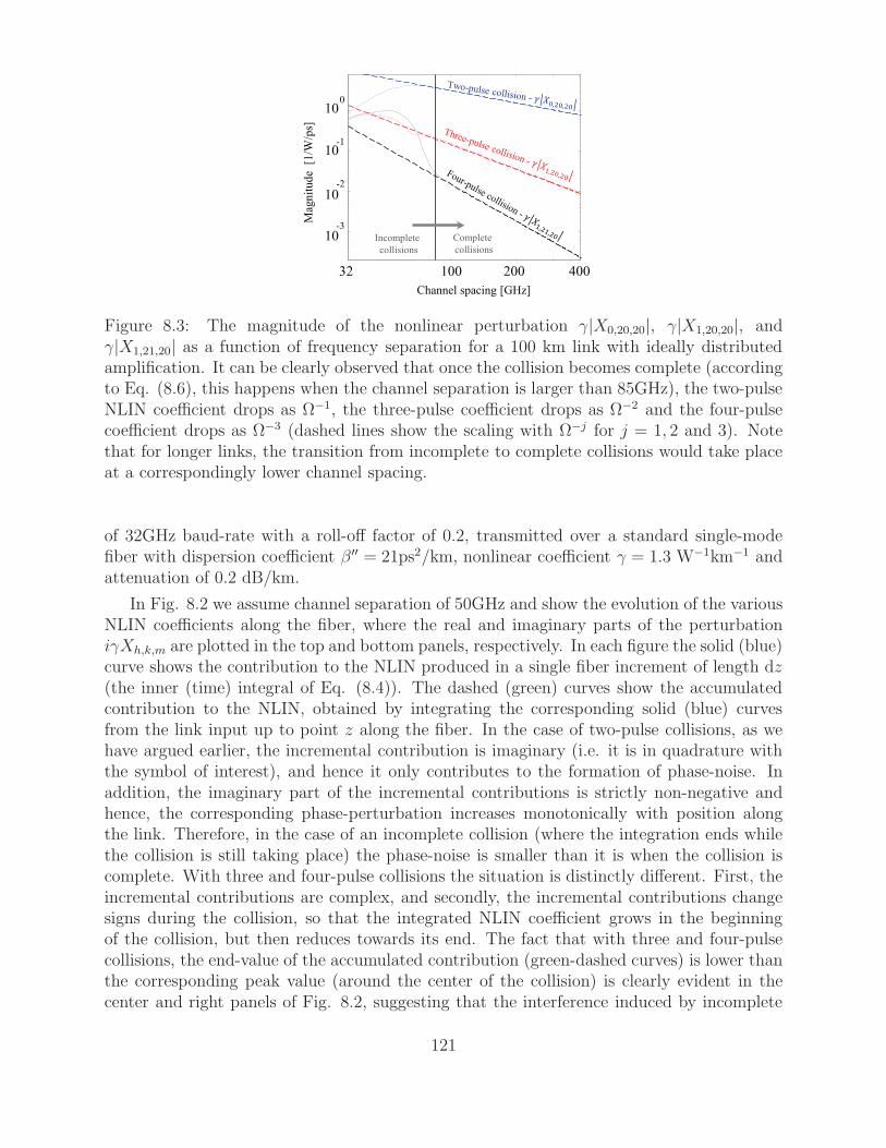
Channel spacing [GHz]

Mag

nit

ude

[1/W

/ps]

32 100 200 400

103-

102-

101-

100

Complete

collisions

Incomplete

collisions

Figure 8.3: The magnitude of the nonlinear perturbation γ|X0,20,20|, γ|X1,20,20|, andγ|X1,21,20| as a function of frequency separation for a 100 km link with ideally distributedamplification. It can be clearly observed that once the collision becomes complete (accordingto Eq. (8.6), this happens when the channel separation is larger than 85GHz), the two-pulseNLIN coefficient drops as Ω−1, the three-pulse coefficient drops as Ω−2 and the four-pulsecoefficient drops as Ω−3 (dashed lines show the scaling with Ω−j for j = 1, 2 and 3). Notethat for longer links, the transition from incomplete to complete collisions would take placeat a correspondingly lower channel spacing.

of 32GHz baud-rate with a roll-off factor of 0.2, transmitted over a standard single-modefiber with dispersion coefficient β ′′ = 21ps2/km, nonlinear coefficient γ = 1.3 W−1km−1 andattenuation of 0.2 dB/km.

In Fig. 8.2 we assume channel separation of 50GHz and show the evolution of the variousNLIN coefficients along the fiber, where the real and imaginary parts of the perturbationiγXh,k,m are plotted in the top and bottom panels, respectively. In each figure the solid (blue)curve shows the contribution to the NLIN produced in a single fiber increment of length dz(the inner (time) integral of Eq. (8.4)). The dashed (green) curves show the accumulatedcontribution to the NLIN, obtained by integrating the corresponding solid (blue) curvesfrom the link input up to point z along the fiber. In the case of two-pulse collisions, as wehave argued earlier, the incremental contribution is imaginary (i.e. it is in quadrature withthe symbol of interest), and hence it only contributes to the formation of phase-noise. Inaddition, the imaginary part of the incremental contributions is strictly non-negative andhence, the corresponding phase-perturbation increases monotonically with position alongthe link. Therefore, in the case of an incomplete collision (where the integration ends whilethe collision is still taking place) the phase-noise is smaller than it is when the collision iscomplete. With three and four-pulse collisions the situation is distinctly different. First, theincremental contributions are complex, and secondly, the incremental contributions changesigns during the collision, so that the integrated NLIN coefficient grows in the beginningof the collision, but then reduces towards its end. The fact that with three and four-pulsecollisions, the end-value of the accumulated contribution (green-dashed curves) is lower thanthe corresponding peak value (around the center of the collision) is clearly evident in thecenter and right panels of Fig. 8.2, suggesting that the interference induced by incomplete

121

Complete

collisions

Incomplete

collisions

m10 20 300

101-

10

100

102-

Mag

nit

ud

e [1

/W/p

s]

(a) 50GHz spacing

Four-pulse collisions

| , , |

Three-pulse collisions

| , , |

Two-pulse collisions

| , , |

m

10 20 300

101-

10

100

102-

103-

40 50

Mag

nit

ud

e [1

/W/p

s]

Complete

collisions

Incomplete

collisions


| , , |


| , , |


| , , |

(b) 100GHz spacing

Figure 8.4: The magnitude of the nonlinear perturbation γ|X0,m,m|, γ|X1,m,m|, andγ|X1,m+1,m| as a function of m for a 100 km link with ideally distributed amplification.Top and bottom panels assume 50GHz and 100GHz channel separations, accordingly. Inlonger links, the transition from incomplete to complete collisions would take place at acorrespondingly higher values of m.

collisions is likely to be much stronger than it is in the case of complete collisions. Thisfeature is particularly strong in the case of four-pulse collisions and for both three-pulse andfour-pulse collisions it becomes increasingly more distinct when the frequency separationbetween the interacting WDM channels becomes larger.

The dependence on frequency separation is illustrated in Fig. 8.3 where we show thedependence of the coefficients Xh,k,m on Ω for a 100 km link. As can be deduced fromAppendix 8.12, when

Ω > B +(m+ k − h)T

2|β ′′|L , (8.6)

where B is the spectral width4 of the individual pulses, the group velocity differences betweenthe channels are large enough to guarantee that the collision is completed before the fiber’send. In the case considered in Fig. 8.3, this happens when the channel spacing is largerthan 85GHz. Evidently, in this regime the perturbation due to two, three, and four-pulse

4We stress that in Eq. (8.6) and throughout this paper Ω and B are indicated in angular frequency units.

122

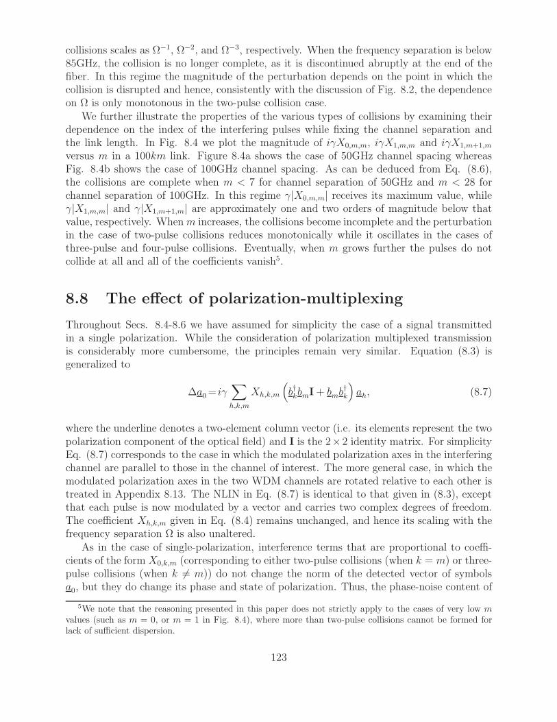
collisions scales as Ω−1, Ω−2, and Ω−3, respectively. When the frequency separation is below85GHz, the collision is no longer complete, as it is discontinued abruptly at the end of thefiber. In this regime the magnitude of the perturbation depends on the point in which thecollision is disrupted and hence, consistently with the discussion of Fig. 8.2, the dependenceon Ω is only monotonous in the two-pulse collision case.

We further illustrate the properties of the various types of collisions by examining theirdependence on the index of the interfering pulses while fixing the channel separation andthe link length. In Fig. 8.4 we plot the magnitude of iγX0,m,m, iγX1,m,m and iγX1,m+1,m

versus m in a 100km link. Figure 8.4a shows the case of 50GHz channel spacing whereasFig. 8.4b shows the case of 100GHz channel spacing. As can be deduced from Eq. (8.6),the collisions are complete when m < 7 for channel separation of 50GHz and m < 28 forchannel separation of 100GHz. In this regime γ|X0,m,m| receives its maximum value, whileγ|X1,m,m| and γ|X1,m+1,m| are approximately one and two orders of magnitude below thatvalue, respectively. Whenm increases, the collisions become incomplete and the perturbationin the case of two-pulse collisions reduces monotonically while it oscillates in the cases ofthree-pulse and four-pulse collisions. Eventually, when m grows further the pulses do notcollide at all and all of the coefficients vanish5.

8.8 The effect of polarization-multiplexing

Throughout Secs. 8.4-8.6 we have assumed for simplicity the case of a signal transmittedin a single polarization. While the consideration of polarization multiplexed transmissionis considerably more cumbersome, the principles remain very similar. Equation (8.3) isgeneralized to

∆a0= iγ∑

h,k,m

Xh,k,m

(b†kbmI+ bmb

†k

)ah, (8.7)

where the underline denotes a two-element column vector (i.e. its elements represent the twopolarization component of the optical field) and I is the 2×2 identity matrix. For simplicityEq. (8.7) corresponds to the case in which the modulated polarization axes in the interferingchannel are parallel to those in the channel of interest. The more general case, in which themodulated polarization axes in the two WDM channels are rotated relative to each other istreated in Appendix 8.13. The NLIN in Eq. (8.7) is identical to that given in (8.3), exceptthat each pulse is now modulated by a vector and carries two complex degrees of freedom.The coefficient Xh,k,m given in Eq. (8.4) remains unchanged, and hence its scaling with thefrequency separation Ω is also unaltered.

As in the case of single-polarization, interference terms that are proportional to coeffi-cients of the form X0,k,m (corresponding to either two-pulse collisions (when k = m) or three-pulse collisions (when k 6= m)) do not change the norm of the detected vector of symbolsa0, but they do change its phase and state of polarization. Thus, the phase-noise content of

5We note that the reasoning presented in this paper does not strictly apply to the cases of very low mvalues (such as m = 0, or m = 1 in Fig. 8.4), where more than two-pulse collisions cannot be formed forlack of sufficient dispersion.

123


= 0, = = 0, 0, 0, =

Two-pulse collisions Three-pulse collisions

Phase-noise and

polarization-rotation

Yes

Circular noise Phase-noise and

polarization-rotation Circular noise

No

• Nature of noise

• Dependence on

modulation format Yes No

• Strongest when the

collision is Complete Incomplete Incomplete Incomplete

Table 8.1: Summary of XPM contributions

NLIN in the single-polarization case is generalized into phase-noise and polarization-rotation.We first show this for the case of two-pulse collisions, whose contribution to the NLIN isgiven by

∆a(2PC)0 = iγ

∑

m

X0,m,m

(‖bm‖2I+ bmb

†m

)a0

=i

2γ∑

m

X0,m,m

(3‖bm‖2I+ ~Bm · ~σ

)a0, (8.8)

where the superscript ‘2PC’ stands for two-pulse-collisions, and where ‖bm‖2 = b†mbm is thesquare modulus of the m-th vector of symbols. The Second line in Eq. (8.8) uses the Stokes-space representation [31]. The term ~σ = (σ1, σ2, σ3) is a vector whose three components are

the Pauli matrices. The term ~Bm is the vector that represents bm in the Stokes space. Itsthree components are real-valued and given by Bm,j = b†mσjbm, with j = 1, 2, or 3. The

notation ~Bm · ~σ is a short-hand for Bm,1σ1 +Bm,2σ2 +Bm,3σ3. All of the relevant propertiesof the Stokes representation are conveniently summarized in [31]. Within the first orderperturbation analysis, the perturbed vector can be written as6

a0 +∆a(2PC)0 = eiϕ2PCe

i2~S2PC·~σa0. (8.9)

where

ϕ2PC =3

2γ∑

m

X0,m,m‖bm‖2 (8.10)

~S2PC = γ∑

m

X0,m,m~Bm. (8.11)

While the first exponent in Eq. (8.9) represents a phase rotation of both polarizations byan angle ϕ2PC, the second exponent represents a polarization-rotation. In the Stokes jargon,the vector representing a0 on the Poincare sphere, rotates about the vector ~S2PC at an angleequal to its length |~S2PC| [31].

As can be readily deduced from Eq. (8.10), the phase-noise ϕ2PC strongly depends on themodulation format, and in particular, its variance vanishes in the case of phase-modulated

6Since the entire theory relies on the first-order perturbation analysis, Eq. (8.9) is not an approximationof Eq. (8.8), but rather it is just as accurate as Eq. (8.8) is.

124

transmission (such as QPSK) as ‖bm‖2 is constant. The dependence of the polarizationrotating effect on modulation format can be seen by observing how the orientation of thevector ~Bm is scattered on the Poincare sphere. In particular, the isotropy of the orientationsof ~Bm on the Poincare sphere increases with increasing QAM-order, whereas with BPSK,or QPSK, all the vectors ~Bm reside in a single plane. Since the polarization-rotation isdetermined by

∑mX0,m,m

~Bm, the variance of the rotations angle |~S2PC| also depends onmodulation format (as shown in the section that follows), but it is always non-zero, even inthe case of pure phase-modulation.

The effect of three-pulse collisions of the type h = 0 and k 6= m generalizes identically tothe above, except that ϕ2PC and ~S2PC are replaced by

ϕ3PC =3

2γ∑

k,mk 6=m

X0,k,mb†kbm (8.12)

~S3PC · ~σ = 2γ∑

k,mk 6=m

X0,k,m

(bmb

†k −

1

2b†kbmI

), (8.13)

where the ‘real-valuedness’ of ϕ3PC and ~S3PC follows from the fact that X0,k,m = X∗0,m,k.

The variance of the phase-shift and of the polarization-rotation angle caused by three-pulsecollisions (k 6= m) are independent of modulation format since bk and bm are statisticallyindependent. The combined perturbation that is caused by both of the above processessatisfies a0 + ∆a

(2PC)0 + ∆a

(3PC)0 = exp(iϕ) exp( i

2~S · ~σ)a0, with ϕ = ϕ2PC + ϕ3PC and ~S =

~S2PC + ~S3PC. The unitarity of these processes implies that ‖a0 +∆a(2PC)0 +∆a

(3PC)0 ‖ = ‖a0‖.

Table 8.1 summarizes the classification of pulse collisions in the polarization multiplexedcase, while pointing out the main properties of each collision type. As seen in the table, theeffects of four-pulse collisions and of three-pulse collisions of the type h 6= 0, k = m remainsunchanged relative to the single-polarization case as they produce complex circular noise oneach of the two polarizations.

It is important to note that the effect of nonlinear polarization-rotation is only unitarywhen both polarization components are considered jointly as a vector. In systems thatprocess the individual polarizations separately, the effect of polarization-rotation does notappear unitary. Rather, from the standpoint of an individual polarization component, thediagonal terms of the polarization-rotation matrix exp( i

2~S · ~σ) appear as additional phase-

noise (which has opposite signs for each of the individual polarization components). Whereas,the non-diagonal terms cause mixing between the two polarization components, which underthe assumption that the components are statistically independent, manifests itself as complexcircular noise. Consequently, in polarization multiplexed systems where the two polarizationchannels are processed separately from each other, two-pulse and three-pulse collisions withh = 0, generate not only pure phase-noise (as in the single-polarization case), but somecomplex circular noise as well. This implies that the relative significance of phase-noise insuch systems is slightly smaller than in the single polarization case.

As explained in Secs. 8.4 and 8.5, and as is summarized in Table 8.1, the dependence ofthe NLIN power on modulation format is caused only by the interference terms proportional

125

to Xh,m,m (whether h = 0, or not)7. In the polarization multiplexed case, the modulationformat dependence of these terms may be slightly weaker than in the case of single polariza-tion. In order to demonstrate this, we examine the NLIN contribution to the y componentof a0 that is proportional to Xh,m,m. This contribution is readily extracted from Eq. (8.7),and it is given by

iγXh,m,m

(2a

(y)h |b(y)m |2 + a

(y)h |b(x)m |2 + a

(x)h b(x)

∗

m b(y)m

). (8.14)

The first term in Eq. (8.14) falls into the category of single polarization interactions and itscontribution to the variance of the NLIN is modulation-format dependent, exactly as dis-cussed in Secs. 8.4-8.5 for the single-polarization case. The same is true for the second termin Eq. (8.14), which represents a classical XPM interaction between the y-polarized symbolsfrom the channel of interest and the x-polarized symbols from the interfering channel. Butthe third term in Eq. (8.14) is different in the sense that it involves interference between fourdifferent data symbols. Assuming that the data transmitted on different polarizations is sta-tistically independent, the variance of the third term is independent of modulation format,and therefore it does not contribute to the modulation format dependence of the overallNLIN variance. It should be noted however, that the modification to the significance ofboth phase-noise (when the polarization channels are processed separately) and modulation-format dependence in polarization multiplexed systems is relatively small, as can be seenin [6] and in the section that follows.

Finally, as we demonstrate in Appendix 8.13, the conclusions of this section do not changewhen the modulated polarization axes in the two channels are not identical. In particular,the phase-noise ϕ, the angle of polarization-rotation |~S|, and the NLIN variance in eachof the two polarizations, are all invariant to whether the modulated polarization axes inthe two WDM channels are identical, or not. A feature that changes somewhat when themodulated polarization axes are different in the two channels, is the relative significance ofphase-noise in systems where the two polarization components are processed separately. Forfurther details, the reader is referred to Appendix 8.13.

8.9 System implications of collision classification

The nature of NLIN in systems changes depending on whether it is dominated by complete orincomplete collisions. A collision can be safely characterized as complete when the evolutionof the individual pulses during the collisions is negligible. This condition can be translatedinto two requirements. The first is that the dispersive broadening of the pulses during thecollision is negligible relative to the pulse width prior to the collisions. This requirement isautomatically satisfied when the frequency spacing between the interacting WDM channelsis sufficiently larger than the bandwidth of the channels themselves. To see that, we definethe collision length, Lc, as the length of the section of fiber in which the collision takes place

7Notice that the variance of the interference contribution that is proportional to Xh,m,m depends on

the statistical average of ‖bm‖4 = |b(y)m |4 + 2|b(y)m |2|b(x)m |2 + |b(x)m |4, where b(y)m and b

(x)m are the y and x

components of bm, accounting for a dependence on the fourth-order moment of the transmitted symbols andfor a dependence on the second-order correlation between the two polarization components.

126

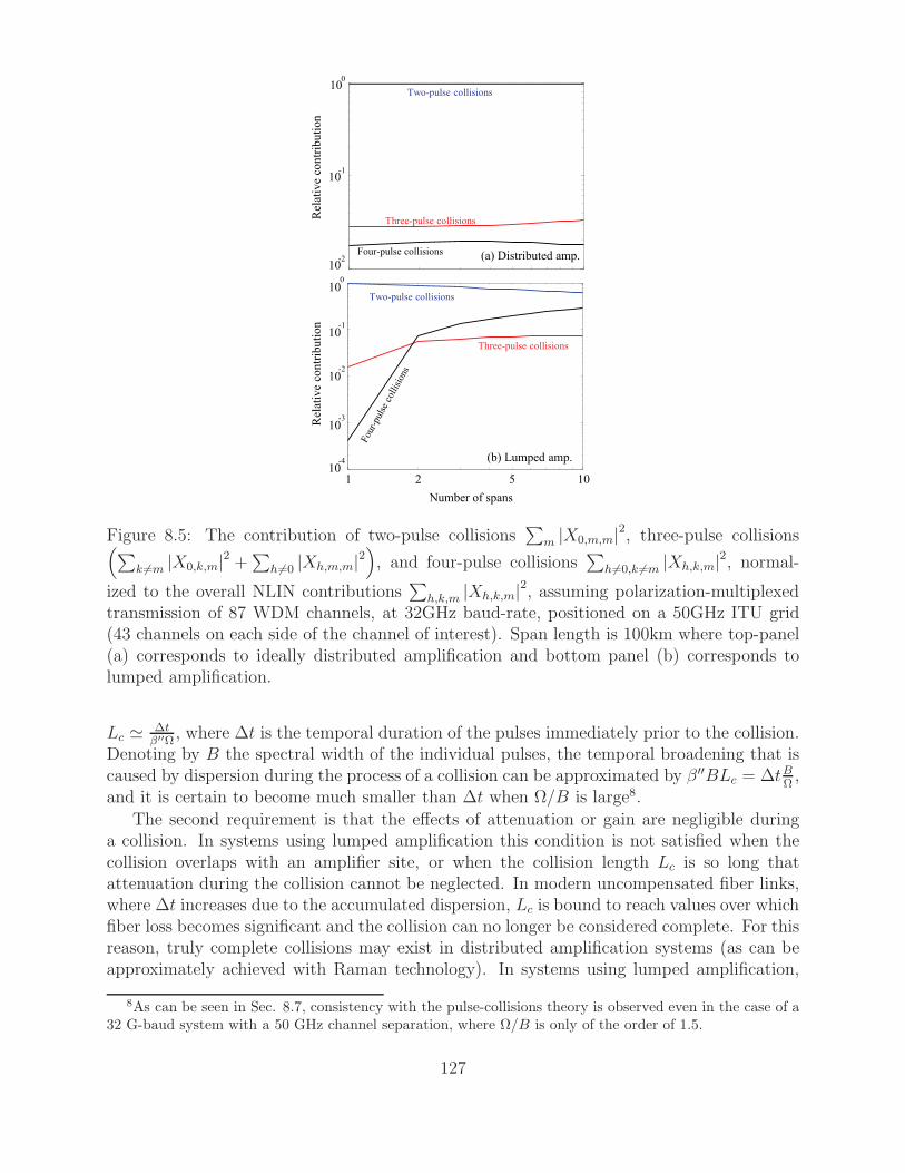
(a) Distributed amp.




102-

101-

100

Rel

ativ

e co

ntr

ibu

tio

n

(b) Lumped amp.



103-

102-

101-

100

Number of spans

Rel

ativ

e co

ntr

ibu

tio

n

2 5 10110

4-

Figure 8.5: The contribution of two-pulse collisions∑

m |X0,m,m|2, three-pulse collisions(∑k 6=m |X0,k,m|2 +

∑h 6=0 |Xh,m,m|2

), and four-pulse collisions

∑h 6=0,k 6=m |Xh,k,m|2, normal-

ized to the overall NLIN contributions∑

h,k,m |Xh,k,m|2, assuming polarization-multiplexedtransmission of 87 WDM channels, at 32GHz baud-rate, positioned on a 50GHz ITU grid(43 channels on each side of the channel of interest). Span length is 100km where top-panel(a) corresponds to ideally distributed amplification and bottom panel (b) corresponds tolumped amplification.

Lc ≃ ∆tβ′′Ω

, where ∆t is the temporal duration of the pulses immediately prior to the collision.Denoting by B the spectral width of the individual pulses, the temporal broadening that iscaused by dispersion during the process of a collision can be approximated by β ′′BLc = ∆tB

Ω,

and it is certain to become much smaller than ∆t when Ω/B is large8.

The second requirement is that the effects of attenuation or gain are negligible duringa collision. In systems using lumped amplification this condition is not satisfied when thecollision overlaps with an amplifier site, or when the collision length Lc is so long thatattenuation during the collision cannot be neglected. In modern uncompensated fiber links,where ∆t increases due to the accumulated dispersion, Lc is bound to reach values over whichfiber loss becomes significant and the collision can no longer be considered complete. For thisreason, truly complete collisions may exist in distributed amplification systems (as can beapproximately achieved with Raman technology). In systems using lumped amplification,

8As can be seen in Sec. 8.7, consistency with the pulse-collisions theory is observed even in the case of a32 G-baud system with a 50 GHz channel separation, where Ω/B is only of the order of 1.5.

127

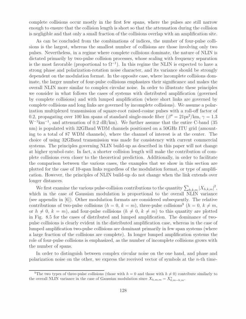
complete collisions occur mostly in the first few spans, where the pulses are still narrowenough to ensure that the collision length is short so that the attenuation during the collisionis negligible and that only a small fraction of the collisions overlap with an amplification site.

As can be concluded from the combinations of indices, the number of four-pulse colli-sions is the largest, whereas the smallest number of collisions are those involving only twopulses. Nevertheless, in a regime where complete collisions dominate, the nature of NLIN isdictated primarily by two-pulse collision processes, whose scaling with frequency separationis the most favorable (proportional to Ω−1). In this regime the NLIN is expected to have astrong phase and polarization-rotation noise character, and its variance should be stronglydependent on the modulation format. In the opposite case, where incomplete collisions dom-inate, the larger number of four-pulse collisions emphasizes their significance and makes theoverall NLIN more similar to complex circular noise. In order to illustrate these principleswe consider in what follows the cases of systems with distributed amplification (governedby complete collisions) and with lumped amplification (where short links are governed bycomplete collisions and long links are governed by incomplete collisions). We assume a polar-ization multiplexed transmission of square-root raised-cosine pulses with a roll-off factor of0.2, propagating over 100 km spans of standard single-mode fiber (β ′′ = 21ps2/km, γ = 1.3W−1km−1, and attenuation of 0.2 dB/km). We further assume that the entire C-band (35nm) is populated with 32GBaud WDM channels positioned on a 50GHz ITU grid (amount-ing to a total of 87 WDM channels), where the channel of interest is at the center. Thechoice of using 32GBaud transmission was made for consistency with current commercialsystems. The principles governing NLIN build-up as described in this paper will not changeat higher symbol-rate. In fact, a shorter collision length will make the contribution of com-plete collisions even closer to the theoretical prediction. Additionally, in order to facilitatethe comparison between the various cases, the examples that we show in this section areplotted for the case of 10-span links regardless of the modulation format, or type of amplifi-cation. However, the principles of NLIN build-up do not change when the link extends overlonger distances.

We first examine the various pulse-collision contributions to the quantity∑

h,k,m |Xh,k,m|2,which in the case of Gaussian modulation is proportional to the overall NLIN variance(see appendix in [6]). Other modulation formats are considered subsequently. The relativecontributions of two-pulse collisions (h = 0, k = m), three-pulse collisions9 (h = 0, k 6= m,or h 6= 0, k = m), and four-pulse collisions (h 6= 0, k 6= m) to this quantity are plottedin Fig. 8.5 for the cases of distributed and lumped amplification. The dominance of two-pulse collisions is clearly evident in the distributed amplification case, whereas in the case oflumped amplification two-pulse collisions are dominant primarily in few span systems (wherea large fraction of the collisions are complete). In longer lumped amplification systems therole of four-pulse collisions is emphasized, as the number of incomplete collisions grows withthe number of spans.

In order to distinguish between complex circular noise on the one hand, and phase andpolarization noise on the other, we express the received vector of symbols at the n-th time-

9The two types of three-pulse collisions (those with h = 0 and those with h 6= 0) contribute similarly tothe overall NLIN variance in the case of Gaussian modulation since Xh,m,m = X∗

0,m−h,m.

128

10-

5-

0

5P

has

e-n

ois

e /

po

lari

zati

on

-ro

tati

on

[d

B]

1 10Number of spans

5215-

Dist. amp.

Lumped amp.

Gaussian

16-QAM

QPSK

(b)

0

5

10

15

20

25

Un

itar

y n

ois

e /

circ

ula

r n

ois

e [d

B]

1 10Number of spans

525-

Dist. amp.

Lumped amp.

Gaussian

16-QAM

QPSK

(a)

Figure 8.6: (a) The ratio between the contribution of unitary noise (phase-noise andpolarization-rotation) and circular noise to the overall NLIN power, i.e. PT (σ2

φ + σ2S)/σ

2ν

in the notation of Eq. (8.16). (b) The ratio between the contributions of phase-noise andpolarization-rotation to the overall NLIN power, i.e. σ2

φ/σ2S. Dotted (red) curves corre-

spond to ideally distributed amplification and solid (black) curves correspond to lumpedamplification, assuming 43 WDM channels on each side of the channel of interest.

slot as

an +∆an = eiφnei2~Sn·~σan + νn (8.15)

where φn represents the phase-noise component of the NLIN, ~Sn is the polarization-rotationvector, as explained in the previous section, and νn represents circular nonlinear noise. Inthe relevant limit of signal to noise ratio being much larger than unity ∆an ≃ i(φnI +12~Sn · ~σ)an + νn and assuming that the data vectors aj and bj are statistically independent,

identically distributed and isotropically symmetric in the phase-space, the NLIN variancecan be expressed as

σ2NLIN = 〈‖∆an‖2〉 − ‖〈∆an〉‖2

= PT (σ2φ + σ2

S) + σ2ν , (8.16)

where σ2φ = 〈φ2

n〉−〈φn〉2, σ2S = 1

4〈|~Sn|2〉, σ2

ν = 〈‖νn‖2〉, P is the average signal power and T isthe symbol duration (so that 〈‖an‖2〉 = PT ). The first two terms on the right-hand-side of

129

the bottom row of Eq. (8.16) are the phase-noise and polarization-rotation contributions tothe total NLIN variance, whereas the third term represents the contribution of the complexcircular noise.

In Fig. 8.6a we plot the ratio between the contributions of the unitary noise (i.e.,phase-noise and polarization-rotation) and of the circular noise to the overall NLIN vari-ance (namely, PT (σ2

φ + σ2S)/σ

2ν). Notice that this ratio is power independent as all the

contributions to the NLIN variance are proportional to P 3. In the distributed amplificationcase, where complete collisions govern the generation of NLIN so that the effect of two-pulsecollisions is dominant, phase-noise and polarization-rotation constitute the largest NLINcontribution, as expected. In the case of lumped amplification, where complete collisionsdominate only the beginning of the link, phase-noise and polarization-rotation are largest af-ter the first amplified span. As the number of spans increases, collisions become increasinglyincomplete and therefore circular noise caused by four-pulse collisions grows gradually.

Figure 8.6b illustrates the relative significance of the two unitary noise contributions,where the ratio σ2

φ/σ2S is plotted versus the number of spans. Clearly, the role of phase-

noise increases with the extent to which the intensity of the symbols is modulated, growingfrom QPSK to 16-QAM and then to Gaussian modulation. This point is further exploredin Fig. 8.7. In addition, in the cases of Gaussian modulation and 16-QAM there is almostno difference between the cases of lumped and distributed amplification, whereas a notabledifference exists in the case of QPSK. The reason is that in QPSK, only three-pulse collisions(of the type h = 0) generate phase-noise and their relative significance increases with thenumber of spans in the case of lumped amplification, whereas it is independent of the link-length in the case of distributed amplification (see Fig. 8.5).

We further address the dependence of the unitary noise and the circular noise on modu-lation format. In order to do that we introduce the concept of the Fourth-order modulationfactor

M =〈|b|4〉〈|b|2〉2 (8.17)

where the random variable b is a symbol in one polarization component of the interferingchannel. The fourth-order modulation factor is equal to unity in the case of pure phase-modulation and grows as the power variations of the modulated signal increase. For examplein the case of QAMmodulation,M = 1 for pure phase modulation (like QPSK) and increasesasymptotically towards 1.4 with the QAM order (specific values are M = 1.32 for 16-QAM,and M = 1.38 for 64-QAM). In the case of complex Gaussian modulation M is equal to2. Excluding cases of extremely tight channel-spacing, which require the correction termdiscussed in [16], and assuming that the two polarization components of the transmitted datavectors are statistically independent, all aspects of the modulation-format dependence of theNLIN power have been shown to be captured by the fourth-order modulation factor [4, 5].

In Fig. 8.7 we plot the contributions of phase-noise PTσ2φ, polarization-rotation PTσ

2S,

and circular noise σ2ν to the NLIN power as a function of M in a 10 × 100km link with

distributed (Fig. 8.7a) and lumped (Fig. 8.7b) amplification. Since the NLIN power scaleswith P 3, the curves are displayed for the case in which P = 1 mW, and therefore to obtainthe results for other input powers, the vertical axes simply need to be shifted upward bythree times the average input power expressed in dBm units. Evidently, the contribution

130

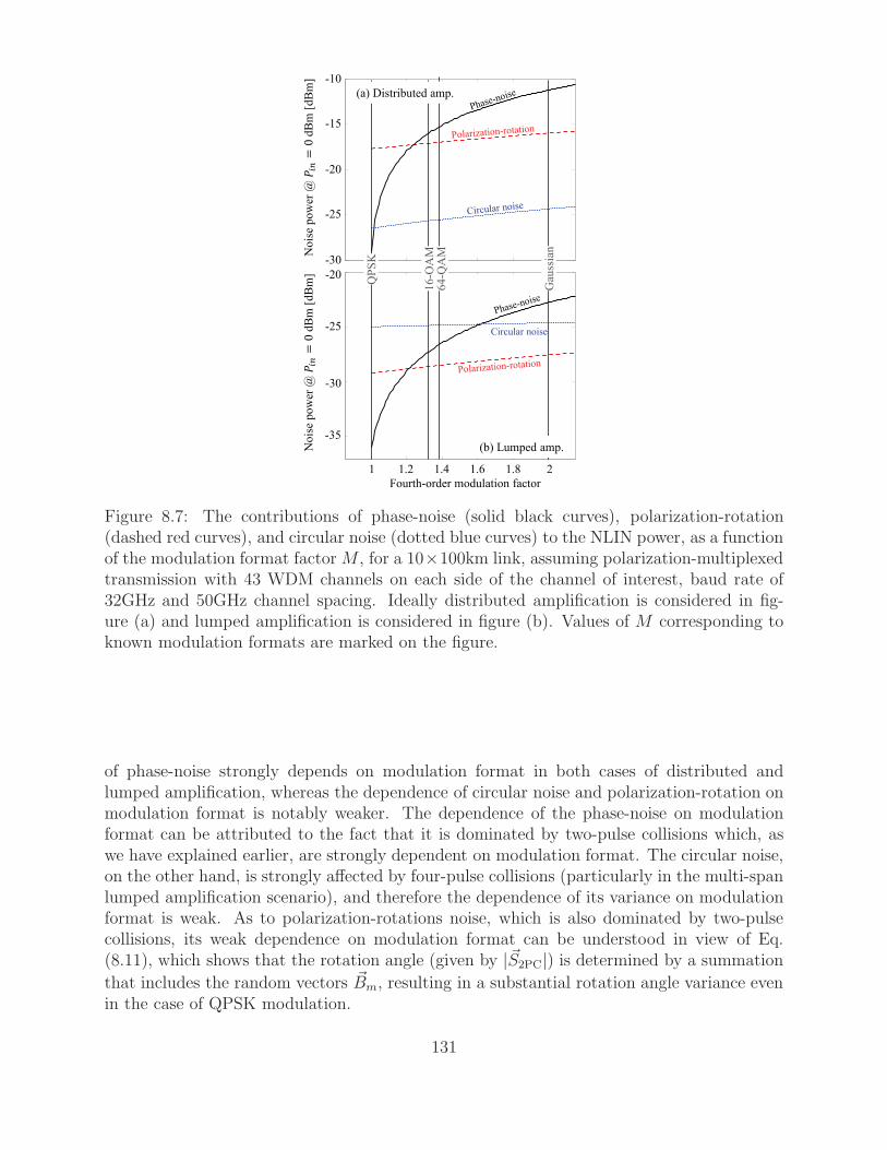
No

ise

po

wer

@

=0

dB

m [

dB

m]

Fourth-order modulation factor

1 1.2 1.4 1.6 1.8 2

No

ise

po

wer

@

=0

dB

m [

dB

m]

35-

30-

20-

30-

10-

25-

25-

15-

20-

(b) Lumped amp.

Circular noise

Gau

ssia

n

QP

SK

16

-QA

M6

4-Q

AM

(a) Distributed amp.

Figure 8.7: The contributions of phase-noise (solid black curves), polarization-rotation(dashed red curves), and circular noise (dotted blue curves) to the NLIN power, as a functionof the modulation format factorM , for a 10×100km link, assuming polarization-multiplexedtransmission with 43 WDM channels on each side of the channel of interest, baud rate of32GHz and 50GHz channel spacing. Ideally distributed amplification is considered in fig-ure (a) and lumped amplification is considered in figure (b). Values of M corresponding toknown modulation formats are marked on the figure.

of phase-noise strongly depends on modulation format in both cases of distributed andlumped amplification, whereas the dependence of circular noise and polarization-rotation onmodulation format is notably weaker. The dependence of the phase-noise on modulationformat can be attributed to the fact that it is dominated by two-pulse collisions which, aswe have explained earlier, are strongly dependent on modulation format. The circular noise,on the other hand, is strongly affected by four-pulse collisions (particularly in the multi-spanlumped amplification scenario), and therefore the dependence of its variance on modulationformat is weak. As to polarization-rotations noise, which is also dominated by two-pulsecollisions, its weak dependence on modulation format can be understood in view of Eq.(8.11), which shows that the rotation angle (given by |~S2PC|) is determined by a summation

that includes the random vectors ~Bm, resulting in a substantial rotation angle variance evenin the case of QPSK modulation.

131

8.10 Relation to the Gaussian noise model and the role

of chromatic dispersion

The GN model has been derived under the assumption that the electric fields of the inter-fering channels are statistically independent Gaussian random processes [26–30]. Hence itspredictions regarding the NLIN power are rigorously accurate (within the obvious limits ofthe first-order perturbation analysis) only when the interfering channels undergo Gaussianmodulation. With other modulation formats, the GN model is known to have certain inaccu-racies, which are particularly conspicuous in the case of distributed amplification systems [4],or few-span systems (less than 1000 km) using lumped amplification [5,6,27]. The improve-ment in the GN model’s accuracy with the number of spans is often attributed to chromaticdispersion [15, 18, 27], with the main argument being that with large chromatic dispersionthe electric fields of the propagating channels approach Gaussian statistics and hence theassumption of Gaussianity, on which the GN model relies, is better satisfied. The difficultywith this argument is that it does not explain the fact that in systems using distributedamplification the inaccuracy of the GN model with non-Gaussian modulation does not seemto reduce with the length of the system [4], regardless of the amount of chromatic dispersionthat the signals accumulate. The role of chromatic dispersion and its relation to the GNmodel’s accuracy can be explained in terms of the pulse collision picture introduced in thispaper, as we elaborate in what follows.

The GN model is accurate in the regime where modulation-format independent threeand four-pulse collisions dominate the formation of NLIN. This does not occur in systemswith distributed amplification, where the completeness of collisions implies that the effects ofthree and four-pulse collisions practically vanishes and the NLIN is dominated by two-pulsecollision processes, independently of the link’s length, as can be seen in Fig. 8.5(a). Inthe regime of lumped optical amplification incomplete collisions become significant to theformation of NLIN only after the first few spans (see Fig. 8.5(b)), which is where the GNmodel’s accuracy begins to improve.

Another interesting aspect of the role of chromatic dispersion has been introduced in [15]and followed in [5]. It has been shown that in the presence of large pre-dispersion thepredictions of the GN model become accurate already in the first span, where in the absenceof pre-dispersion the GN model is known to be highly inaccurate. It has been suggested [15]that the better accuracy of the GN model in this case results from the fact that pre-dispersiontransforms the distribution of the electric field of the interfering channels into Gaussian,independently of their modulation format. While tempting in its simplicity, this argumentis inconsistent with an observation that was reported in [5], where it was shown that theinaccuracy of the predictions of the GN model in pre-dispersed systems is smaller thanwithout pre-dispersion only in short links whose accumulated dispersion is much smallerthan the pre-dispersion that was applied. For example, when the interfering channels arepre-dispersed by an amount equivalent to 500 km of transmission fiber, the GN model’sprediction improved in the first few hundred kilometers, but in longer links, of the orderof 1000 km, it deteriorated to the same level of inaccuracy characterizing systems withoutpre-dispersion, as illustrated in Fig. 5 of [5]. Clearly, if the GN model’s accuracy improvedbecause of better Gaussianity that followed from pre-dispersion, there is no reason for it

132

to deteriorate in longer systems, where even more dispersion is accumulated. The theorypresented in this paper suggests a different explanation, that was briefly alluded to in [5].Large pre-dispersion creates overlaps between all pulses at the link input so that the collisionstaking place in the first few spans of the systems are incomplete. The incompleteness of thecollisions emphasizes the significance of modulation format independent three and four-pulsecollisions whose effect tends to agree with the predictions of the GN model. As the systembecomes longer, the impact of pre-dispersion reduces and the inaccuracy of the GN modelresumes its regular value.

8.11 Conclusions

We have shown that the various contributions to inter-channel NLIN can be classified aspulse collisions involving two, three, or four colliding pulses. Furthermore, we have arguedthat pulse collisions may either be complete (if they occur on a length-scale where loss/gainand dispersive broadening are negligible), or incomplete. When the majority of collisions arecomplete (as occurs with distributed gain systems [4] or in few-span systems using lumpedamplification [5]) the NLIN is dominated by two-pulse collisions which give it the characterof phase-noise and polarization-rotation noise with strong dependence on modulation for-mat. When the majority of collisions are incomplete (high span-count systems with lumpedamplification), the role of four-pulse interactions becomes more prominent, emphasizing thecircular NLIN component, as assumed in [26–30]. In this case the dependence of NLIN onthe modulation format is much weaker.

Acknowledgement

The authors would like to acknowledge financial support from the Israel Science Foundation(grant 737/12). Ronen Dar would like to acknowledge the support of the Adams Fellowship ofthe Israel Academy of Sciences and Humanities, the Yitzhak and Chaya Weinstein ResearchInstitute and the Advanced Communication Center and the Electro-Optic Fund of Tel-AvivUniversity.

8.12 Appendix: The dependence on Ω in complete ver-

sus incomplete collisions

We consider a generic setup of the kind plotted in Fig. 8.1. Two pulses, with indices 0 andh, belonging to the channel of interest collide with two pulses of the interfering channel,whose indices are k and m. Recall that the pulse with the index 0 is not a real pulse thatpropagates along the fiber, but rather (as we described earlier) it is included in the analysisso as to account for the effect of matched filtering.

We assume the regime of large accumulated dispersion, which is relevant in the case of

133

dispersion uncompensated links and take advantage of the far-field approximation [4, 10],

g(z, t) ≃√

i

2π |β ′′| z exp(− it2

2β ′′z

)g

(t

β ′′z

), (8.18)

where g(ω) =∫g(t) exp(iωt)dt is the Fourier transform of the fundamental waveform g(t).

By substituting Eq. (8.18) into Eq. (8.4) and using the change of variables ω = t/β ′′z, weget

Xh,k,m≃ eiΩhT

2π |β ′′|

∫ z1

z0

f(z)

zψ(Ω + mT

β′′z

)eimTβ′′z

hTdz, (8.19)

where m stands for (m+ k − h)/2 and

ψ(u)=1

2π

∫ ∞

−∞g∗(ω + u+ hT

2β′′z

)g(ω + u− hT

2β′′z

)

× g∗(ω + (m−k)T

2β′′z

)g(ω − (m−k)T

2β′′z

)

× eiω(h−k+m)Tdω. (8.20)

Note that the function ψ(u) reduces to zero when z satisfies |h|T2|β′′|z > B

2or |m−k|T

2|β′′|z > B2,

where B is the spectral width of the fundamental pulse g(t). In the limit of large dispersion,

we can assume that |m−k|T2|β′′|z ≪ B

2so that the product g∗

(ω + (m−k)T

2β′′z

)g(ω − (m−k)T

2β′′z

)is

approximately equal to |g (ω)|2. In the same manner, by assuming |h|T2|β′′|z ≪ B

2we get

ψ(u) ≃ 1

2π

∫ ∞

−∞|g (ω + u)|2 |g (ω)|2 eiω(h−k+m)Tdω. (8.21)

Since ψ(u) ≃ 0 when |u| ≤ B we can conclude that the lower integration limit z0 in Eq.

(8.19) is the largest of the three quantities |h|T|β′′|B ,

|k−m|T|β′′|B , and mT

|β′′|(Ω+B), whereas the upper

limit z1 is the smaller between the link length L and mT|β′′|(Ω−B)

. These integration limits z0 andz1 can be intuitively understood when considering the nature of the nonlinear interaction, asillustrated in Fig. 8.1. In the general case, two pulses from the channel of interest interactwith two pulses of the interfering channel, and the nonlinear interaction takes place while allfour pulses overlap with each other temporally. The dispersive broadening of the individualpulses after propagating to point z along the fiber is approximately |β ′′|Bz. Within thefar field approximation, significant overlap between the zeroth and the h-th pulses in thechannel of interest is achieved when |β ′′|Bz ≫ |h|T and similarly the k-th and m-th pulsesin the interfering channel overlap when |β ′′|Bz ≫ |m − k|T . In this case, the zeroth andh-th pulses form a single block of width ∼ |β ′′|Bz centered at hT/2, whereas the k-th andm-th pulses form a block of the same width, centered at (m + k)T/2 − βΩz. The overlapbetween the two blocks starts when (m+k)T/2−βΩz−β ′′Bz/2 > hT/2+β ′′Bz/2 and endswhen (m+ k)T/2− βΩz + β ′′Bz/2 < hT/2− β ′′Bz/2. The combination of these conditionstranslates into the integration limits indicated above, implying that when h, k and m satisfym > max|h| , |k −m|(1+Ω/B), a collision is formed if the condition m < (Ω+B) |β ′′|L/T

134

is being satisfied. The collision is completed before the end of the link if h, k and m furthersatisfy m < (Ω−B) |β ′′|L/T .

Finally, defining u = Ω + mTβ′′z

, Eq. (8.19) can be rewritten as

Xh,k,m =1

2π |β ′′|

∫ u1

u0

1

Ω− uf(

mT|β′′|(Ω−u)

)e−iuhT ψ(u)du, (8.22)

where u0 = Ω + mTβ′′z1

and u1 = Ω+ mTβ′′z0

. This form will be useful in what follows.

8.12.1 Complete collisions

In the case of a complete collision, the integrand in Eq. (8.22) vanishes at the integrationboundaries, which can therefore be replaced by ±∞. In addition, since in the regime ofcomplete collisions, attenuation and gain during the collision must be assumed negligible,

we may replace f(

mT|β′′|(Ω−u)

)with f

(mT|β′′|Ω

)and move it outside of the integral. Having done

so, we obtain

Xh,k,m=f(

mT|β′′|Ω

)

2π |β ′′|Ω∞∑

n=0

∫ ∞

−∞

un

Ωne−iuhT ψ(u)du. (8.23)

Defining ψ(v) = 12π

∫∞−∞ ψ(u) exp(−iuv)du, as the inverse Fourier transform of ψ(u), Eq.

(8.23) can be rewritten as

Xh,k,m=1

|β ′′|Ωf(

mT|β′′|Ω

) ∞∑

n=0

(i

Ω

)n

ψ(n)(hT ), (8.24)

where ψ(n)(hT ) is the n-th derivative of ψ(v), evaluated at v = hT . From Eq. (8.21) it isevident that

ψ(v) = R∗(v)R(v − (h− k +m)T

), (8.25)

where R(v) =∫g∗(t)g(v − t)dt is the temporal autocorrelation function of the fundamental

pulse g(t). The orthogonality condition of Eq. (8.2) implies that R(v) has a maximum whenv = 0 (R(0) = 1) and that it vanishes when v/T is any integer other than 0.

It is evident from Eq. (8.25) that the only contribution that scales with Ω−1 is theone proportional to ψ(0)(hT ) = ψ(hT ). Substitution of v = hT in Eq. (8.25) reveals thatψ(hT ) = R∗(hT )R

((k − m)T

)is non-zero only when h = 0 and k = m. This is exactly

the case of two-pulse collisions discussed earlier. The next contribution to NLIN, whichscales as Ω−2, follows from ψ(1)(hT ) = R′(hT )R

((k − m)T

)+ R(hT )R′((k − m)T

)and it

is nonzero only in the case of three-pulse collisions with h = 0 and k 6= m (one pulse inthe channel of interest and two pulses in the interfering channel), or with h 6= 0 and k = m(two pulses in the channel of interest and a single pulse in the interfering channel). Only theterm with n = 2 in the summation in Eq. (8.24), which scales as Ω−3 is nonzero in the caseof complete four-pulse collisions (with h 6= 0 and k 6= m). Hence we may summarize thatcomplete two-pulse collisions scale as Ω−1, complete three-pulse collisions scale as Ω−2 and

135

complete four-pulse collisions scale as Ω−3. As can be deduced from the integration limitsof Eq. (8.22), the number of complete two, three and four-pulse collisions is proportionalto Ω, Ω2 and Ω3, respectively, and therefore their overall contribution to NLIN (which isproportional to |Xh,k,m|2) is dominated by two-pulse collisions (see Sec. 8.7).

8.12.2 Incomplete collisions

The analysis of incomplete collisions is somewhat more complicated and difficult to extendbeyond what is given by expressions (8.19), or (8.22). Some insight can be gained fromconsidering the case of distributed amplification where f(z) = 1 and can be taken out of theintegral. In this case Eq. (8.23) still holds, except that the actual integration limits u0 to u1need to be applied.

Using the formulation of the previous subsection ψ(v) is no longer given by Eq. (8.25), butrather it is the convolution of the expression on the right-hand-side of Eq. (8.25) with a sincfunction corresponding to the inverse Fourier transform of a unit frequency window extendingbetween u0 and u1. In this situation ψ(hT ) may differ from zero for all combinations of h, k,and m, implying that the contributions of all types of incomplete pulse collisions scale asΩ−1.

8.13 Appendix: Relative rotation between the modu-

lated polarization axes of the interacting WDM

channels

In the analysis of polarization multiplexing in Sec. 8.8, we assumed for simplicity that themodulated polarization axes in the interfering channel are parallel to those in the channelof interest. This assumption clearly does not represent the situation in reality where themodulated polarization axes in each of the two channels undergo different paths betweenthe individual transmitters and the point at which they are wavelength multiplexed into asingle transmission fiber. In addition, polarization mode dispersion in practical links mayalso cause relative polarization rotations between the various WDM channels. We examinethese situations in this appendix.

Rigorously, the rotation of relative polarizations can be taken into account by replacingthe vectors bj with Ubj , where U is an arbitrary unitary matrix representing a relativerotation between the channel of interest and the interfering channel, changing the expressionfor the NLIN into

∆a0= iγ∑

h,k,m

Xh,k,mU(b†kbmI+ bmb

†k

)U†ah. (8.26)

According to Eq. (8.26), and by assuming that the components of aj and bj are isotropic intheir phase-space, the NLIN variance is given by

〈‖∆a0‖2〉−‖〈∆a0〉‖2

= γ2∑

h,k,mh′,k′,m′

X∗h,k,mXh′,k′,m′〈a†hΛ†

k,mΛk′,m′ah′〉, (8.27)

136

where Λk,m = U(b†kbmI+ bmb

†k − 〈b†kbmI+ bmb

†k〉)U†, and the subtraction of the average

〈b†kbmI + bmb†k〉 inside the parenthesis eliminates the average (deterministic) phase shift of

the entire constellation10. By further assuming that the polarization components of aj andbj are statistically independent and identically distributed, it can be readily shown that

〈a†hΛ†k,mΛk′,m′ah′〉 is zero whenever h′ 6= h, k′ 6= k, or m′ 6= m, meaning that the NLIN

variance is

〈‖∆a0‖2〉−‖〈∆a0〉‖2

= γ2∑

h,k,m

〈a†hΛ†k,mΛk,mah〉|Xh,k,m|2

=γ2∑

h,k,m

Tr(〈Λk,maha

†hΛ

†k,m〉

)|Xh,k,m|2

=γ2〈|a|2〉∑

h,k,m

〈Tr(Λk,mΛ

†k,m

)〉|Xh,k,m|2, (8.28)

where Tr(A) denotes the trace of the matrix A. Finally, since the trace of a matrix isinvariant to unitary rotations, i.e. Tr

(UAU†) = Tr (A), Eq. (8.28), and therefore also the

NLIN variance, are independent of the relative rotation between the channels. Notice thatsymmetry between the two polarization components suggests that the NLIN variance in eachpolarization component is also invariant to U.

Further insight into the effect of relative polarization rotation can be extracted from Eq.(8.15), which describes the effect of nonlinearity as a phase-noise φn, polarization-rotation

noise ~Sn, and circular noise νn. The variance of the circular noise νn is independent of U,as discussed in the previous paragraph. In addition, using Eqs. (8.10-8.13) it can be easily

verified that both the phase shift φn and the rotation angle |~Sn| are also independent of U.Yet, in cases where the two polarization channels are processed separately from each other,the inclusion of U may affect the phase-noise that is observed in each of the individualpolarization components. This can be seen most conveniently from the contribution of two-pulse collisions to the phase-noise in the y component of the vector a0, which are givenby

γ∑

m

X0,m,m

(2|b(y)m |2 + |b(x)m |2

), (8.29)

where b(x)m and b

(y)m are the x and y component of the vector Ub, respectively. Assume for

simplicity the example of phase-modulated transmission (e.g. QPSK) where there is no

rotaion of the relative modulation axes (U = I). In this case |b(x)m |2 = |b(y)m |2 = Const and thevariance of the phase-noise due to the contribution of two-pulse collisions is 0. In the casewhere U 6= I, |b(x)m |2 and |b(y)m |2 become dependent on the transmitted data so that two-pulsecollisions contribute to a phase-noise with nonzero variance.

10The subtracted sum iγ∑

h,k,m Xh,k,mU〈b†kbmI+ bmb†k〉U†ah represents a deterministic phase-shift whenk = m and h = 0. The summation over the terms k 6= m is clearly 0 because of the statistical independencebetween symbols and their isotropy. The summation over the terms h 6= 0 can also be shown to be 0 byusing the property that

∑m Xh,m,m = 0 for all h 6= 0.

137

Bibliography

[1] R.-J. Essiambre, G. Kramer, P.J. Winzer, G.J. Foschini, B. Goebel, “Capacity limits ofoptical fiber networks,” J. Lightwave Technol., vol. 28, pp. 662–701 (2010).

[2] A. Mecozzi, C. B. Clausen, and M. Shtaif, “Analysis of intrachannel nonlinear effects inhighly dispersed optical pulse transmission,” IEEE Photon. Technol. Lett., vol 12, pp.392-394 (2000).

[3] F. Forghieri, R.W. Tkack, A. R. Chraplyvy, “Fiber nonlinearities and their impact ontransmission systems,” Ch. 8 in Optical Fiber Telecommunications IIIA, P. Kaminowand T. L. Koch eds. (Academic Press, 1997).



[6] R. Dar, M. Feder, A. Mecozzi, M. Shtaif, “Inter-channel nonlinear interference noisein WDM systems: modeling and mitigation,” accepted for publication in J. LightwaveTechnol. (October 2014).

[7] R. Dar, M. Shtaif, M. Feder, “New bounds on the capacity of the nonlinear fiber-opticchannel,” Optics Lett., vol. 39, pp. 398–401 (2014).

[8] R. Dar, M. Feder, A. Mecozzi, M. Shtaif, “Time varying ISI model for nonlinear inter-ference noise,” in Optical Fiber Communication (OFC) Conference, pp. W2A.62, SanFrancisco (2014).


[10] A. Mecozzi and R.-J. Essiambre, “Nonlinear Shannon limit in pseudolinear coherentsystems,” J. Lightwave Technol., vol. 30, pp. 2011–2024 (2012).

[11] S. Kumar, D. Yang, “Second-order theory for self-phase modulation and cross-phasemodulation in optical fibers,” J. Lightwave Technol., vol. 23, pp. 2073–2080 (2005).

138

[12] S. N. Shahi, S. Kumar, X. Liang, “Analytical modeling of cross-phase modulation incoherent fiber-optic system,” Optics express, vol. 22, pp. 1426–1439 (2014).

[13] X. Liang, S. Kumar, “Analytical modeling of XPM in dispersion-managed coherentfiber-optic systems,” Optics Express, vol. 22, pp. 10579–10592 (2014).

[14] A. Mecozzi and F. Matera, “Polarization scattering by intra-channel collisions,” OpticsExpress, vol. 20, pp. 1213–1218 (2012).

[15] A. Carena, G. Bosco, V. Curri, P. Poggiolini, F. Forghieri, “Impact of the transmittedsignal initial dispersion transient on the accuracy of the GN-model of non-linear propa-gation,” in European Conference on Optical Communication (ECOC), Paper Th.1.D.4,London (2013).


[17] N. Rossi, P. Ramantanis, J.-C. Antona, “Nonlinear interference noise statistics in un-managed coherent networks with channels propagating over different lightpaths,” inEuropean Conference on Optical Communications (ECOC), Paper Mo.4.3.4, Cannes(2014).

[18] P. Serena, A. Bononi, “On the accuracy of the Gaussian nonlinear model for dispersion-unmanaged coherent links,” in European Conference on Optical Communications(ECOC), Paper Th.1.D.3, London (2013).

[19] L. F. Mollenauer, S. G Evangelides, J.P. Gordon, “Wavelength division multiplexingwith solitons in ultra-long distance transmission using lumped amplifiers,” J. LightwaveTechnol., vol. 9, pp. 362–367 (1991)

[20] S. G. Evangelides Jr, J. P. Gordon, “Energy transfers and frequency shifts from threesoliton collisions in a multiplexed transmission line with periodic amplification,” J.Lightwave Technol., vol. 14, pp. 1639–1643 (1996).

[21] J. F. L. Devaney, W. Forysiak, A. M. Niculae, N. J. Doran, “Soliton collisions indispersion-managed wavelength-division-multiplexed systems,” Optics Lett.,vol. 22, pp.1695–1697 (1997)

[22] P. V. Mamyshev and L. F. Mollenauer, “Soliton collisions in wavelength-division-multiplexed dispersion-managed systems,” Optics Lett.,vol. 24, pp. 448–450 (1999)

[23] M. Shtaif, “Analytical description of cross-phase modulation in dispersive optical fibers.”Optics Lett., vol. 23, pp. 1191–1193 (1998).

[24] J. Bromage, “Raman amplification for fiber communications systems,” J. LightwaveTechnol., vol 22, p. 79 (2004).

[25] F. Forghieri, R. W. Tkach, A. R. Chraplyvy, “Fiber nonlinearities and their impact ontransmission system,” in Optical Fiber Telecommunications IIIA, I.P. Kaminow and T.L. Koch eds., Academic (1997)

139

[26] P. Poggiolini, A. Carena, V. Curri, G. Bosco, F. Forghieri, “Analytical modeling ofnonlinear propagation in uncompensated optical transmission links,” IEEE Photon.Technol. Lett., vol. 23, pp. 742–744 (2011).

[27] A. Carena, V. Curri, G. Bosco, P. Poggiolini, F. Forghieri, “Modeling of the impact ofnonlinear propagation effects in uncompensated optical coherent transmission links,” J.Lightwave Technol., vol. 30, pp. 1524–1539 (2012).

[28] P. Poggiolini, “The GN model of non-linear propagation in uncompensated coherentoptical systems,” J. Lightwave Technol., vol. 30, pp. 3857-3879 (2012).

[29] P. Johannisson and M. Karlsson, “Perturbation analysis of nonlinear propagation in astrongly dispersive optical communication system,” IEEE J. Lightwave Technol., vol.31, pp. 1273–1282 (2013).

[30] P. Serena, A. Bononi, “An alternative approach to the Gaussian noise model and itssystem implications,” J. Lightwave Technol., vol 31, pp. 3489–3499 (2013).

[31] J. P. Gordon and H. Kogelnik, “PMD fundamentals: Polarization mode dispersion inoptical fibers,” Proc. Natl. Acad. Sci. USA, vol. 97, pp. 4541-4550 (2000).

140

Chapter 9

Shaping in the Nonlinear Fiber-Optic

Channel

9.1 Channel model

We consider a WDM transmission where several channels are launched into a nonlinearoptical fiber. The received signal at the n-th time-slot in the channel of interest is given by

yn = an +∆an + zn , (9.1)

where an is the data symbol transmitted over the channel of interest at the n-th symbol time,and where ∆an is the interference induced by the nonlinearity of the fiber. The amplifiedspontaneous emission (ASE) noise in the system is represented by zn and is modeled as alinear additive white complex Gaussian noise with zero mean and variance σ2

ASE.In Eq. (9.1) we assume that the channel of interest has been back-propagated so as to

eliminate the intra-channel nonlinearities, implying that only inter-channel interference isincluded in ∆an

1. The interference resulting from a single interfering channel was shown tohave the form (see Chapter 4)

∆an =∑

l,k,m

an−lb∗n−kbn−mXl,k,m. (9.2)

The symbol bn is the n-th data symbol of the interfering channel and Xl,k,m is a coefficientwhose explicit form is provided in Chapter 4 and whose value is defined by the waveformsof the individual pulses, the channel separation, the dispersion coefficient, the link distanceand the link power loss/gain profile. For simplicity of notation, Eq. (9.2) was written forthe case of a single interfering channel, whereas in the presence of multiple interferers ∆anis approximately equal to the sum of the individual contributions2.

1The analysis presented in this chapter can be derived in a similar way also for intra-channel nonlinearities.In fact, these NLIN contributions may also be suppressed by spherical constellations. The investigation ofthe achievable shaping gains resulting from both intra- and inter-channel NLIN suppression is left for futurestudy.

2Four-wave mixing effects, i.e. nonlinear interactions that do not involve the channel of interest, andnonlinear interactions of ASE noise with itself and with the signal, are considered to be much smaller thanthose discussed here.

141

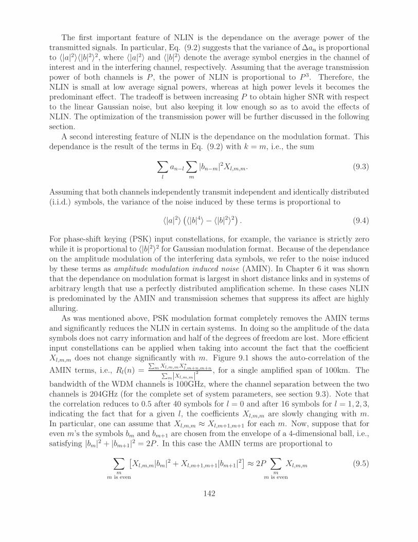
The first important feature of NLIN is the dependance on the average power of thetransmitted signals. In particular, Eq. (9.2) suggests that the variance of ∆an is proportionalto 〈|a|2〉〈|b|2〉2, where 〈|a|2〉 and 〈|b|2〉 denote the average symbol energies in the channel ofinterest and in the interfering channel, respectively. Assuming that the average transmissionpower of both channels is P , the power of NLIN is proportional to P 3. Therefore, theNLIN is small at low average signal powers, whereas at high power levels it becomes thepredominant effect. The tradeoff is between increasing P to obtain higher SNR with respectto the linear Gaussian noise, but also keeping it low enough so as to avoid the effects ofNLIN. The optimization of the transmission power will be further discussed in the followingsection.

A second interesting feature of NLIN is the dependance on the modulation format. Thisdependance is the result of the terms in Eq. (9.2) with k = m, i.e., the sum

∑

l

an−l

∑

m

|bn−m|2Xl,m,m. (9.3)

Assuming that both channels independently transmit independent and identically distributed(i.i.d.) symbols, the variance of the noise induced by these terms is proportional to

〈|a|2〉(〈|b|4〉 − 〈|b|2〉2

). (9.4)

For phase-shift keying (PSK) input constellations, for example, the variance is strictly zerowhile it is proportional to 〈|b|2〉2 for Gaussian modulation format. Because of the dependanceon the amplitude modulation of the interfering data symbols, we refer to the noise inducedby these terms as amplitude modulation induced noise (AMIN). In Chapter 6 it was shownthat the dependance on modulation format is largest in short distance links and in systems ofarbitrary length that use a perfectly distributed amplification scheme. In these cases NLINis predominated by the AMIN and transmission schemes that suppress its affect are highlyalluring.

As was mentioned above, PSK modulation format completely removes the AMIN termsand significantly reduces the NLIN in certain systems. In doing so the amplitude of the datasymbols does not carry information and half of the degrees of freedom are lost. More efficientinput constellations can be applied when taking into account the fact that the coefficientXl,m,m does not change significantly with m. Figure 9.1 shows the auto-correlation of the

AMIN terms, i.e., Rl(n) =∑

m Xl,m,mX∗l,m+n,m+n

∑m|Xl,m,m|2 , for a single amplified span of 100km. The

bandwidth of the WDM channels is 100GHz, where the channel separation between the twochannels is 204GHz (for the complete set of system parameters, see section 9.3). Note thatthe correlation reduces to 0.5 after 40 symbols for l = 0 and after 16 symbols for l = 1, 2, 3,indicating the fact that for a given l, the coefficients Xl,m,m are slowly changing with m.In particular, one can assume that Xl,m,m ≈ Xl,m+1,m+1 for each m. Now, suppose that foreven m’s the symbols bm and bm+1 are chosen from the envelope of a 4-dimensional ball, i.e.,satisfying |bm|2 + |bm+1|2 = 2P . In this case the AMIN terms are proportional to

∑

mm is even

[Xl,m,m|bm|2 +Xl,m+1,m+1|bm+1|2

]≈ 2P

∑

mm is even

Xl,m,m (9.5)

142

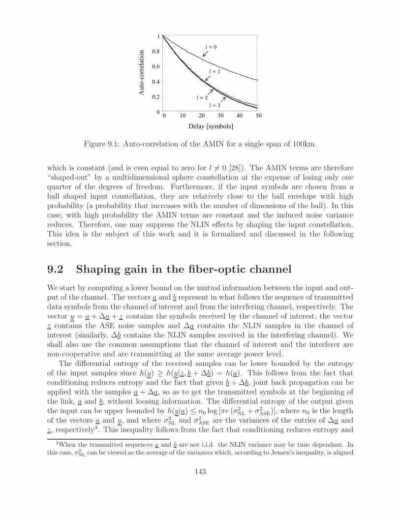
0 10 20 30 40 500

0.2

0.4

0.6

0.8

1

Delay [symbols]

Au

to-c

orr

elat

ion

= 0

= 1

= 2

= 3

Figure 9.1: Auto-correlation of the AMIN for a single span of 100km.

which is constant (and is even equal to zero for l 6= 0 [28]). The AMIN terms are therefore“shaped-out” by a multidimensional sphere constellation at the expense of losing only onequarter of the degrees of freedom. Furthermore, if the input symbols are chosen from aball shaped input constellation, they are relatively close to the ball envelope with highprobability (a probability that increases with the number of dimensions of the ball). In thiscase, with high probability the AMIN terms are constant and the induced noise variancereduces. Therefore, one may suppress the NLIN effects by shaping the input constellation.This idea is the subject of this work and it is formalized and discussed in the followingsection.

9.2 Shaping gain in the fiber-optic channel

We start by computing a lower bound on the mutual information between the input and out-put of the channel. The vectors a and b represent in what follows the sequence of transmitteddata symbols from the channel of interest and from the interfering channel, respectively. Thevector y = a + ∆a + z contains the symbols received by the channel of interest, the vectorz contains the ASE noise samples and ∆a contains the NLIN samples in the channel ofinterest (similarly, ∆b contains the NLIN samples received in the interfering channel). Weshall also use the common assumptions that the channel of interest and the interferer arenon-cooperative and are transmitting at the same average power level.

The differential entropy of the received samples can be lower bounded by the entropyof the input samples since h(y) ≥ h(y|z, b + ∆b) = h(a). This follows from the fact thatconditioning reduces entropy and the fact that given b+∆b, joint back propagation can beapplied with the samples a +∆a, so as to get the transmitted symbols at the beginning ofthe link, a and b, without loosing information. The differential entropy of the output giventhe input can be upper bounded by h(y|a) ≤ n0 log [πe (σ

2NL + σ2

ASE)], where n0 is the lengthof the vectors a and y, and where σ2

NL and σ2ASE are the variances of the entries of ∆a and

z, respectively3. This inequality follows from the fact that conditioning reduces entropy and

3When the transmitted sequences a and b are not i.i.d. the NLIN variance may be time dependant. Inthis case, σ2

NL can be viewed as the average of the variances which, according to Jensen’s inequality, is aligned

143

the fact that Gaussian distribution maximizes the differential entropy of a random variablewith a given covariance matrix.

The resultant lower bound on the mutual information of the channel is therefore

1

n0I(a; y) ≥ 1

n0h(a)− log

[πe(σ2NL + σ2

ASE

)](9.6)

We note that this bound may be loose to some extent as we have applied some relaxing as-sumptions along the way. In particular, the bound on h(y|a) assumes that the NLIN samples,∆a, are memoryless, statistically independent of a and follow a Gaussian distribution. Asdiscussed in the previous sections, in some scenarios the memoryless assumption is not toorestrictive. In the case of short links, for example, the dynamics of NLIN are fast changingand the memory property cannot be exploited to enhance the information rates. Secondly,the assumption of statistical independence between NLIN and the input samples is a strictlyrestrictive assumption, as the dependance can be clearly observed in Eq. (9.2). The thirdassumption, on the Gaussianity of the NLIN, is not too harsh since each sample of NLINinvolves many independent nonlinear interactions and therefore it is indeed approximatelypoint-wise Gaussian. In addition, the lower bound on h(y) assumes that the entropy ofthe received samples is dominated by the entropy of the input samples. This assumptionhowever is well justified in the regimes of interest, namely at the high SNR regime wherethe average input power is much larger than the ASE noise as well as the NLIN (as can beseen from Fig. 9.3b).

Upon reviewing the assumptions above, we stress that the resulted bound on the mutualinformation may be relatively loose. It allows us, however, to derive some very interest-ing insights on the ability to shape the input constellation not only to reduce the averagetransmission power but also to “shape-out” the nonlinear interference. The lower boundpresented in Eq. (9.6) further allows us to derive an analytical expression for the achievableshaping gain in the fiber-optic channel, an expression that accounts also for the dependanceof NLIN on the input constellation. In what follows we compute the bound in Eq. (9.6) forthe cases of uniform input distribution within a 2N -dimensional cube and ball, and derivean analytical expression for the shaping gain in the fiber-optic channel.

9.2.1 2N-dimensional cube

Let the data symbols of the channel of interest and the interfering channel be uniformlydistributed over a 2N -dimensional cube. In order to compute the lower bound of Eq. (9.6)we need to derive the entropy of the input distribution and the induced NLIN variance. Thelatter is given by

σ2NL = P 3X1 + P 3

( 〈|b0|4〉〈|b0|2〉2

− 2

)X2 (9.7)

where we used the fact that the symbols al and bm are i.i.d. and statistically independentof each other, and where we denote the quantities

∑l,k,m |Xl,k,m|2 and

∑l,m |Xl,m,m|2 by X1

and X2, respectively. The quantity K = 〈|b0|4〉/〈|b0|2〉2 − 2 accounts for the dependance

with our goal of upper bounding the entropy h(y|a).

144

on the fourth order moment (that implies a dependance on the amplitude modulation ofthe interfering symbols), and in our case it is equal to -0.6. For 4-QAM and 16-QAMconstellations, K is equal to -1 and -0.68, respectively, whereas it approaches to -0.6 as thesize of the QAM constellation increases.

The entropy of a random vector that is uniformly distributed within some multi-dimensionalregion is equal to the logarithm of the region volume [46]. The entropy of the input in ourcase is therefore log(6P ) and the resulting lower bound on the mutual information follows

1

n0I(a; y) ≥ log

(6

πe

P

σ2ASE + P 3

(X1 − 0.6X2

))

. (9.8)

The optimal average transmission power is the one that optimally accounts both for the linearand nonlinear noises and maximizes the mutual information at the output of the channel.The average power that maximizes the expression on the right hand side of Eq. (9.8) (andactually maximizes the effective SNR at the receiver) is equal to

P ⊡

opt =

(1

2

σ2ASE

X1 − 0.6X2

)1/3

, (9.9)

and the maximum mutual information is hereby bounded by

I ⊡

max , supP

1

n0

I(a; y) ≥ log

(4

πe

P ⊡

opt

σ2ASE

). (9.10)

9.2.2 2N-dimensional ball

In the case of uniform input distribution within a 2N -dimensional ball, the input symbolsare statistically dependant and using straight forward calculations the NLIN variance canbe shown to satisfy

σ2NL = P 3 〈|b0|2|b1|2〉

〈|b0|2〉2X1

+ P 3

(〈|b0|4〉 − 〈|b0|2|b1|2〉〈|b0|2〉2

− 1

)X2

+ P 3

(〈|b0|2|b1|2〉〈|b0|2〉2

− 1

)XCOV (9.11)

where b0 and b1 are two correlated input symbols and the term XCOV is given by

XCOV = 2∑

l,s

(s+1)N−2∑

m=sN

(s+1)N−1∑

k=m+1

ReXl,m,mX∗l,k,k . (9.12)

Now, suppose that each M consecutive coefficients Xl,m,m, ..., Xl,m+M−1,m+M−1 are ap-proximately equal. In this case, if N ≤M then

XCOV ≈ (N − 1)∑

l,m

|Xl,m,m|2 = (N − 1)X2 . (9.13)

145

If N > M , then XCOV is approximately equal to (M − 1)X24. By using straightforward

calculations we find that 〈|b0|4〉 = 2P 2(N +1)/(N +2) and 〈|b0|2|b1|2〉 = P 2(N +1)/(N +2),and the NLIN variance follows

σ2NL ≈ P 3N + 1

N + 2X1 − P 3 M

N + 2X2 (9.14)

where M = minN,M.Since the volume of the ball is V2N(P ) = (π(N +1)P )N/N ! and the entropy of the input

is log (V2N(P )) we get that the optimal average power is

P⊙

opt =

(1

2

σ2ASE

N+1N+2

X1 − MN+2

X2

)1/3

(9.15)

and the lower bound on the maximum mutual information is

I ⊙

max , supP

1

n0

I(a; y) ≥ log

(2(N + 1)

3e(N !)1/NP ⊙

opt

σ2ASE

). (9.16)

9.2.3 Shaping gain

In fiber-optic systems one can arbitrarily choose the average transmission power, and so wewould like to compare the maximum information rate of the various input distributions. Thedifference between the bounds on the maximum mutual information of a uniform distributionwithin a 2N -dimensional ball and within a cube is given by

I ⊙

max − I ⊡

max = log

(π(N + 1)

6(N !)1/NP ⊙

opt

P ⊡

opt

). (9.17)

Notice that the first quotient in the expression inside the logarithm is exactly the shaping gainof a 2N -dimensional ball in the linear AWGN channel. The second quotient accounts for thefact that the optimal average power depends on the NLIN variance which is affected by theshaping of the input constellation. Hence, on the one hand, shaping the input constellationmay reduce the average power of the transmitted symbols, and on the other hand, it mayreduce the NLIN variance and therefore increase the optimal average power.

We therefore can write the shaping gain in the optical fiber channel as

γOFCs (⊙) = γAWGN

s (⊙) γNLs (⊙) (9.18)

where γAWGNs (⊙) is the shaping gain of a 2N -dimensional ball in the AWGN channel and

where γNLs (⊙) is the gain from “shaping-out” the NLIN. By plugging the optimal average

power levels from Eqs. (9.9) and (9.15) we get that the latter is given by

γNLs (⊙) =

(X1 − 0.6X2

N+1N+2

X1 − MN+2

X2

)1/3

(9.19)

4A more precise expression should also account for the cross terms Xl,m,mX∗l,k,k with |k − m| > M ,

however, the significance of these terms is relatively small when M is chosen to be large enough.

146

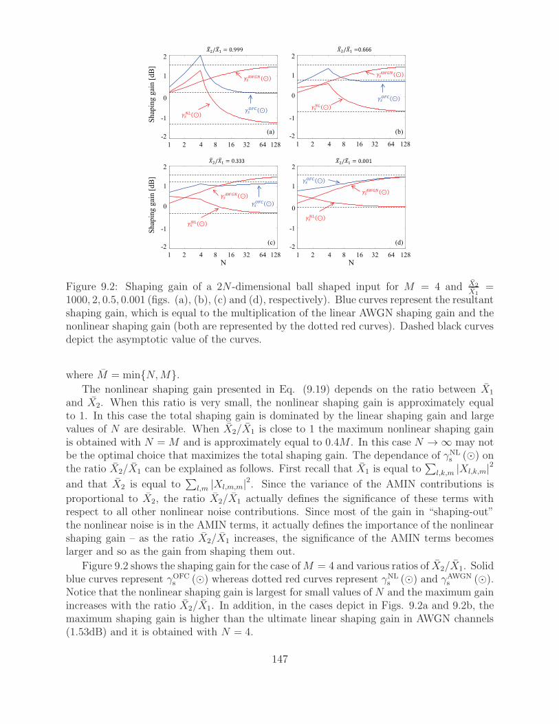
Sh

apin

g g

ain

[d

B]

2

1

0

-1

-2

1 4 16 64 1283282

2

1

0

-1

-2

1 4 16 64 1283282

(a) (b)

Sh

apin

g g

ain

[d

B]

2

1

0

-1

-2

1 4 16 64 1283282

(c)

N

2

1

0

-1

-2

1 4 16 64 1283282

(d)

N

/ = 0.999 / =0.666

/ = 0.333 / = 0.001

Figure 9.2: Shaping gain of a 2N -dimensional ball shaped input for M = 4 and X2

X1=

1000, 2, 0.5, 0.001 (figs. (a), (b), (c) and (d), respectively). Blue curves represent the resultantshaping gain, which is equal to the multiplication of the linear AWGN shaping gain and thenonlinear shaping gain (both are represented by the dotted red curves). Dashed black curvesdepict the asymptotic value of the curves.

where M = minN,M.The nonlinear shaping gain presented in Eq. (9.19) depends on the ratio between X1

and X2. When this ratio is very small, the nonlinear shaping gain is approximately equalto 1. In this case the total shaping gain is dominated by the linear shaping gain and largevalues of N are desirable. When X2/X1 is close to 1 the maximum nonlinear shaping gainis obtained with N =M and is approximately equal to 0.4M . In this case N → ∞ may notbe the optimal choice that maximizes the total shaping gain. The dependance of γNL

s (⊙) onthe ratio X2/X1 can be explained as follows. First recall that X1 is equal to

∑l,k,m |Xl,k,m|2

and that X2 is equal to∑

l,m |Xl,m,m|2. Since the variance of the AMIN contributions is

proportional to X2, the ratio X2/X1 actually defines the significance of these terms withrespect to all other nonlinear noise contributions. Since most of the gain in “shaping-out”the nonlinear noise is in the AMIN terms, it actually defines the importance of the nonlinearshaping gain – as the ratio X2/X1 increases, the significance of the AMIN terms becomeslarger and so as the gain from shaping them out.

Figure 9.2 shows the shaping gain for the case ofM = 4 and various ratios of X2/X1. Solidblue curves represent γOFC

s (⊙) whereas dotted red curves represent γNLs (⊙) and γAWGN

s (⊙).Notice that the nonlinear shaping gain is largest for small values of N and the maximum gainincreases with the ratio X2/X1. In addition, in the cases depict in Figs. 9.2a and 9.2b, themaximum shaping gain is higher than the ultimate linear shaping gain in AWGN channels(1.53dB) and it is obtained with N = 4.

147

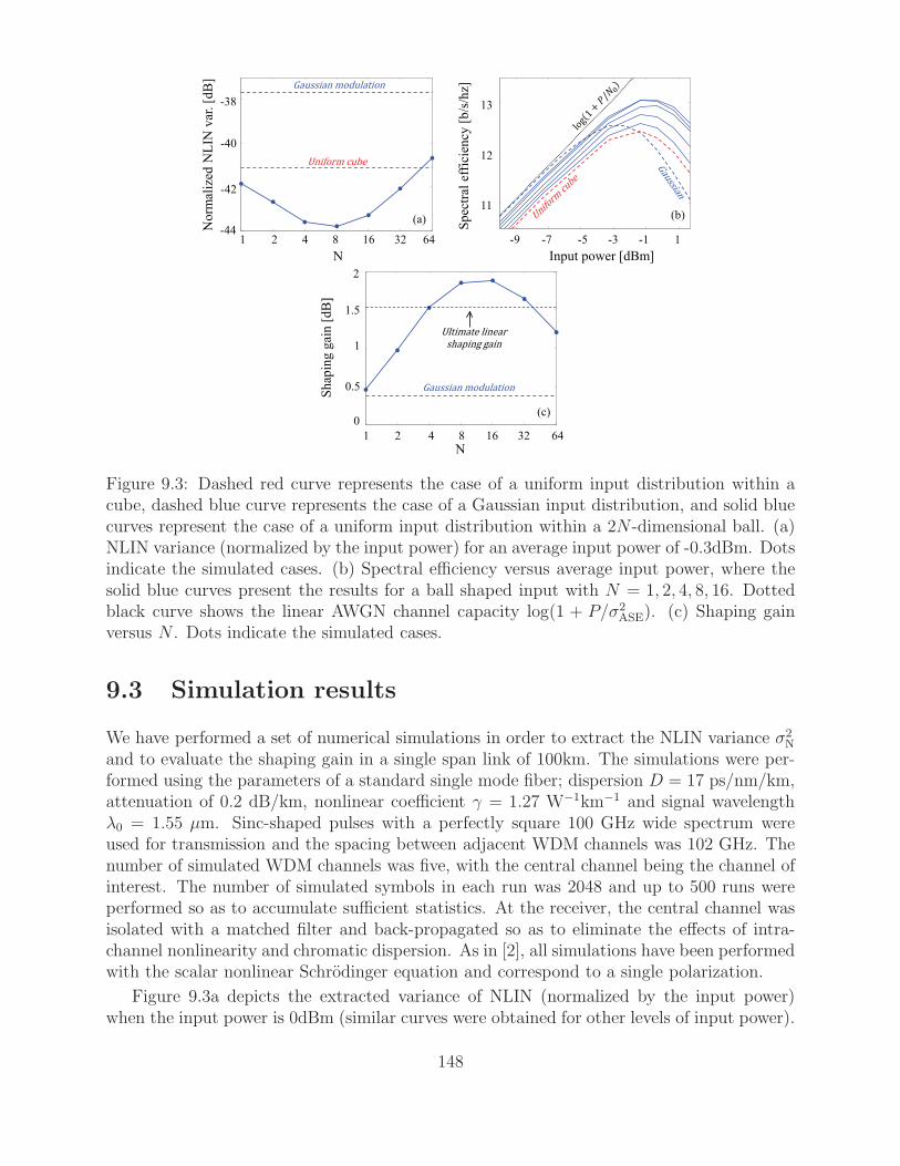
11

12

13

Sp

ectr

al e

ffic

ien

cy [

b/s

/hz]

9- 7- 5- 3- 1- 1

Input power [dBm]

(b)

44-

42-

40-

No

rmal

ized

NL

IN v

ar.

[dB

]

1 2 4 8 16 32

N

64

38-

Gaussian modulation

Uniform cube

(a)

0

0.5

1

Sh

apin

g g

ain

[d

B]

1 2 4 8 16 32

N64

1.5

2

Gaussian modulation

(c)

Ultimate linear shaping gain

Figure 9.3: Dashed red curve represents the case of a uniform input distribution within acube, dashed blue curve represents the case of a Gaussian input distribution, and solid bluecurves represent the case of a uniform input distribution within a 2N -dimensional ball. (a)NLIN variance (normalized by the input power) for an average input power of -0.3dBm. Dotsindicate the simulated cases. (b) Spectral efficiency versus average input power, where thesolid blue curves present the results for a ball shaped input with N = 1, 2, 4, 8, 16. Dottedblack curve shows the linear AWGN channel capacity log(1 + P/σ2

ASE). (c) Shaping gainversus N . Dots indicate the simulated cases.

9.3 Simulation results

We have performed a set of numerical simulations in order to extract the NLIN variance σ2N

and to evaluate the shaping gain in a single span link of 100km. The simulations were per-formed using the parameters of a standard single mode fiber; dispersion D = 17 ps/nm/km,attenuation of 0.2 dB/km, nonlinear coefficient γ = 1.27 W−1km−1 and signal wavelengthλ0 = 1.55 µm. Sinc-shaped pulses with a perfectly square 100 GHz wide spectrum wereused for transmission and the spacing between adjacent WDM channels was 102 GHz. Thenumber of simulated WDM channels was five, with the central channel being the channel ofinterest. The number of simulated symbols in each run was 2048 and up to 500 runs wereperformed so as to accumulate sufficient statistics. At the receiver, the central channel wasisolated with a matched filter and back-propagated so as to eliminate the effects of intra-channel nonlinearity and chromatic dispersion. As in [2], all simulations have been performedwith the scalar nonlinear Schrodinger equation and correspond to a single polarization.

Figure 9.3a depicts the extracted variance of NLIN (normalized by the input power)when the input power is 0dBm (similar curves were obtained for other levels of input power).

148

Dashed red curve represent the case of a uniform input distribution within a cube, solid bluecurve represents the case of a uniform input distribution within a 2N -dimensional ball (dotsindicate the simulated cases), and dashed blue curve represents the case of a Gaussian inputdistribution (equivalent to the case of N → ∞. Evidently, a ball shaped input with N = 8attains the smallest NLIN variance, a value which is smaller by 2.7dB and 6.1dB than theNLIN variance for the case of uniform input distribution within a cube and a Gaussian inputdistribution, respectively.

In Fig. 9.3b we use the extracted NLIN variances in order to compute the lower bound onthe mutual information given by (9.6), where we draw only the curves ofN = 1, 2, 4, 8, 16. Forlow levels of average input power the nonlinear effects are small and the fiber-optic channel isapproximately a linear AWGN channel. In this regime the mutual information in the case ofa Gaussian input distribution is identical to the linear capacity and the mutual informationin the case of a uniform distribution within a cube approaches to the linear capacity up tothe ultimate shaping gain of 1.53dB. For higher levels of average input power, the nonlineareffects become stronger and limits the achievable information rates. The maximum spectralefficiency is obtained with a ball shaped input of N = 16. Note that the maximum spectralefficiency is notably higher than the maximum spectral efficiency obtained with a Gaussianinput.

Figure 9.3c shows the resultant shaping gain, i.e., 2Id where Id is the difference between themaximum mutual information obtained by the various input distributions and the maximummutual information obtained by the uniform distribution within a cube. The maximumshaping gain is obtained with N = 16 – while the case of Gaussian input distribution obtainsonly a 0.38dB shaping gain, a ball shaped input with N = 16 obtains a gain of 1.88dB whichis clearly better than the 1.53dB ultimate shaping gain in a linear AWGN channel.

149

Chapter 10

Summary and Conclusions

In the context of SDM transmission in fiber-optic communications, we have studied theunder-addressed optical MIMO channel, where the number of fiber modes addressed bythe transmitter and receiver is allowed to be smaller than the overall number of modesexisting in the fiber. This scenario was motivated by the idea of installing fibers that admitmore modes than can be processed with currently available technology, mainly in orderto achieve future-proof operation [14]. By establishing the relation between the channelssingular values and the Jacobi ensemble of random matrices we derived the ergodic capacity,outage probability and optimal diversity-multiplexing tradeoff. An interesting phenomenonis observed when the parameters of the model satisfy mt +mr > m (where m is the totalnumber of modes that are available in the fiber, and where mt and mt are the number ofmodes that are addressed by the transmitter and receiver, respectively): for any realizationof the transfer matrix, mt+mr−m singular values are 1. This results in an ergodic capacitywhich is at least mt + mr − m times the SISO capacity. In the non-ergodic scenario thisenables a strictly zero outage probability and an exponentially decaying error probability(“infinite diversity”) for any transmission rate below (mt + mr − m)log(1 + SNR). Theresults of Chapters 2 and 3 therefore quantify the information theoretical limits of opticalSDM systems with respect to m, mt and mr and they may be used to understand thetradeoff between system performance and the complexity and cost that come along with theutilization of more modes. For example, one important outcome that may be relevant alsofor SDM systems that address most of the available modes, is the fact that a performanceequivalent of mt+mr−m uncoupled single-mode channels is always achievable. It should benoted however that Chapters 2 and 3 study the information theoretical limitations imposedby not addressing all modes while ignoring the limitations imposed by the nonlinearity ofthe fiber. The impact of nonlinearities on the results of Chapters 2 and 3 is left for futureresearch.

The main focus of my PhD research was the modeling problem of nonlinear propagationin fiber-optic communications. We have reviewed the essential parts of two previous modelingapproaches, the time domain model and the frequency domain GN model, and pointed outthe differences between the models. We have shown that by correctly accounting for fourth-order correlations in the NLIN spectrum an extra term arises. The inclusion of this termrecovers the dependence of the NLIN power on modulation format, a property that is absentfrom the existing GN model and reconciles between the frequency domain and the time

151

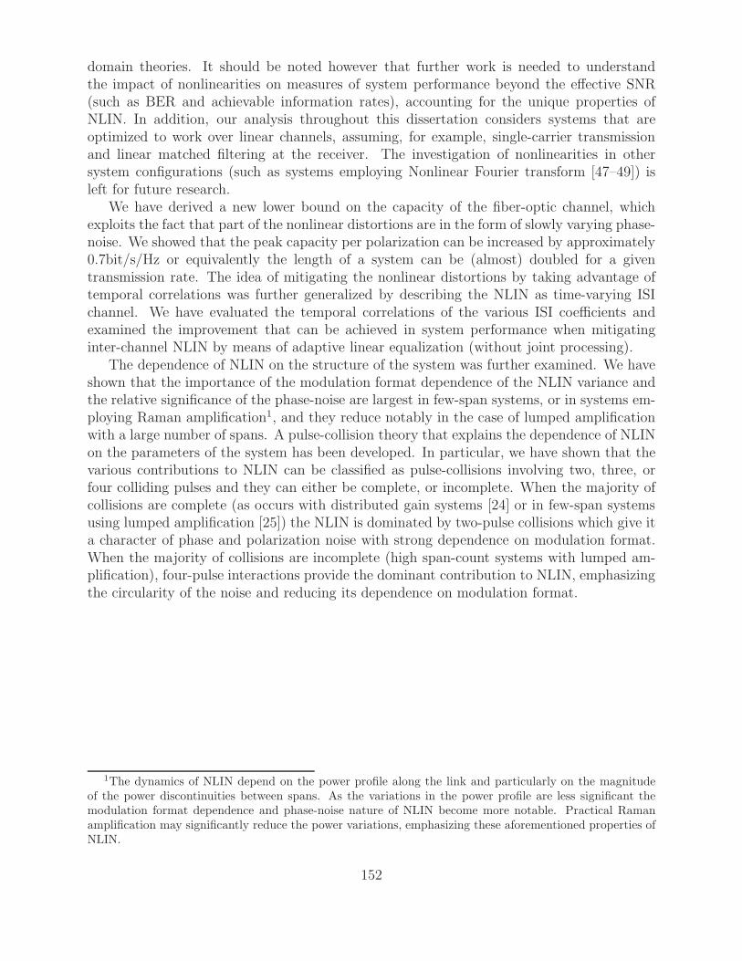
domain theories. It should be noted however that further work is needed to understandthe impact of nonlinearities on measures of system performance beyond the effective SNR(such as BER and achievable information rates), accounting for the unique properties ofNLIN. In addition, our analysis throughout this dissertation considers systems that areoptimized to work over linear channels, assuming, for example, single-carrier transmissionand linear matched filtering at the receiver. The investigation of nonlinearities in othersystem configurations (such as systems employing Nonlinear Fourier transform [47–49]) isleft for future research.

We have derived a new lower bound on the capacity of the fiber-optic channel, whichexploits the fact that part of the nonlinear distortions are in the form of slowly varying phase-noise. We showed that the peak capacity per polarization can be increased by approximately0.7bit/s/Hz or equivalently the length of a system can be (almost) doubled for a giventransmission rate. The idea of mitigating the nonlinear distortions by taking advantage oftemporal correlations was further generalized by describing the NLIN as time-varying ISIchannel. We have evaluated the temporal correlations of the various ISI coefficients andexamined the improvement that can be achieved in system performance when mitigatinginter-channel NLIN by means of adaptive linear equalization (without joint processing).

The dependence of NLIN on the structure of the system was further examined. We haveshown that the importance of the modulation format dependence of the NLIN variance andthe relative significance of the phase-noise are largest in few-span systems, or in systems em-ploying Raman amplification1, and they reduce notably in the case of lumped amplificationwith a large number of spans. A pulse-collision theory that explains the dependence of NLINon the parameters of the system has been developed. In particular, we have shown that thevarious contributions to NLIN can be classified as pulse-collisions involving two, three, orfour colliding pulses and they can either be complete, or incomplete. When the majority ofcollisions are complete (as occurs with distributed gain systems [24] or in few-span systemsusing lumped amplification [25]) the NLIN is dominated by two-pulse collisions which give ita character of phase and polarization noise with strong dependence on modulation format.When the majority of collisions are incomplete (high span-count systems with lumped am-plification), four-pulse interactions provide the dominant contribution to NLIN, emphasizingthe circularity of the noise and reducing its dependence on modulation format.

1The dynamics of NLIN depend on the power profile along the link and particularly on the magnitudeof the power discontinuities between spans. As the variations in the power profile are less significant themodulation format dependence and phase-noise nature of NLIN become more notable. Practical Ramanamplification may significantly reduce the power variations, emphasizing these aforementioned properties ofNLIN.

152

Bibliography

[1] P. P. Mitra and J. B. Stark, “Nonlinear limits to the information capacity of opticalfibre communications,”Nature, vol. 411, pp. 1027–1030 (2001).

[2] R.-J. Essiambre, G. Kramer, P.J. Winzer, G.J. Foschini, B. Goebel, “Capacity limits ofoptical fiber networks,” Journal of Lightwave Technology, vol. 28, pp. 662–701 (2010).

[3] K. S. Turitsyn, S. A. Derevyanko, I. V. Yurkevich, and S. K. Turitsyn, “Informationcapacity of optical fiber channels with zero average dispersion,”Physical review letters,vol. 91, pp. 203901–203904 (2003).

[4] M. Secondini, E. Forestieri, G. Prati, “Achievable information rate in nonlinear WDMfiber-optic systems with arbitrary modulation formats and dispersion maps,” Journalof Lightwave Technology, vol. 31, pp. 3839–3852 (2013).

[5] E. Agrell and M. Karlsson, “WDM channel capacity and its dependence on multichanneladaptation models,”in Optical Fiber Communication (OFC) conference, pp. OTu3B-4,Anaheim, CA (2013).

[6] A. Carena, V. Curri, G. Bosco, P. Poggiolini, and F. Forghieri, “Modeling of the impactof nonlinear propagation effects in uncompensated optical coherent transmission links,”Journal of Lightwave Technology, vol. 30, pp. 1524–1539 (2012).

[7] P. Serena, A. Bononi, “An alternative approach to the Gaussian noise model and itssystem implications,” Journal of Lightwave Technology, vol 31, pp. 3489–3499 (2013).

[8] S. N. Shahi, S. Kumar, X. Liang, “Analytical modeling of cross-phase modulation incoherent fiber-optic system,” Optics express, vol. 22, pp. 1426–1439 (2014).

[9] E. Agrell, “The channel capacity increases with power,” arXiv preprint:1108.0391(2011).

[10] S. Berdague and P. Facq, “Mode division multiplexing in optical fibers,”Applied Optics,vol. 21 pp. 1950–1955 (1982).

[11] A. Tarighat, R. C. Hsu, A. Shah, A. H. Sayed, and B. Jalali, “Fundamentals andchallenges of optical multiple-input multiple-output multimode fiber links,”IEEE Com-munications Magazine, vol. 45 (2007).

153

[12] R. W. Tkach, “Scaling optical communications for the next decade and beyond,” BellLabs Technical Journal, vol. 14, pp. 3–9 (2010).

[13] A. Chralyvy, “The coming capacity crunch,” in European Conference on Optical Com-munication (ECOC), plenary paper, Vienna (2009).

[14] P. J. Winzer and G. J. Foschini, “MIMO capacities and outage probabilities in spatiallymultiplexed optical transport systems,”Optics Express, vol. 19, pp. 16680–16696 (2011).

[15] R. Dar, M. Feder, A. Mecozzi, and M. Shtaif, “On shaping gain in the nonlinear fiber-optic channel,” in IEEE International Symposium on Information Theory (ISIT), pp.2794–2798, Honolulu (2014).

[16] R. J. Muirhead, “Aspects of Multivariate Statistical Theory.” Wiley (1982).

[17] M. L Mehta , “Random Matrices.” Academic Press (1991).

[18] A. Edelman and N. R. Rao, “Random matrix theory,” Acta Numerica, vol. 14, pp.233–297 (2005).

[19] A. Mecozzi, C. B. Clausen, and M. Shtaif, “Analysis of intrachannel nonlinear effects inhighly dispersed optical pulse transmission,” IEEE Photonics Technology Letters, vol12, pp. 392-394 (2000).

[20] F. Forghieri, R.W. Tkack, A. R. Chraplyvy, “Fiber nonlinearities and their impacton transmission systems,” Chapter 8 in Optical Fiber Telecommunications IIIA, P.Kaminow and T. L. Koch eds., Academic Press (1997).

[21] E. Ip, J.M. Kahn “Compensation of dispersion and nonlinear impairments using digitalbackpropagation,” Journal of Lightwave Technology, vol. 26, pp. 3416–3425 (2008).

[22] R. I. Killey, P. M. Watts, V. Mikhailov, M. Glick, P. Bayvel “Electronic dispersioncompensation by signal predistortion using digital processing and a dual-drive Mach-Zehnder modulator,” IEEE Photonics Technology Letters, vol. 17, pp. 714–716 (2005).

[23] E. Ip, “Nonlinear compensation using backpropagation for polarization-multiplexedtransmission,” Journal of Lightwave Technology, vol 28, pp. 939–951 (2010).



[26] R. Dar, M. Feder, A. Mecozzi, M. Shtaif, “Inter-channel nonlinear interference noise inWDM systems: modeling and mitigation,” Journal of Lightwave Technology, vol. 33,pp. 1044–1053 (2015).

[27] R. Dar, M. Shtaif, M. Feder, “New bounds on the capacity of the nonlinear fiber-opticchannel,” Optics Letters, vol. 39, pp. 398–401 (2014).

154

[28] R. Dar, M. Feder, A. Mecozzi, M. Shtaif, “Time varying ISI model for nonlinear inter-ference noise,” in Optical Fiber Communication (OFC) conference, pp. W2A.62, SanFrancisco, CA (2014).


[30] R. Dar, M. Feder, A. Mecozzi, M. Shtaif, “Pulse collision picture of inter-channel non-linear interference noise in fiber-optic communications,” accepted for publication inJournal of Lightwave Technology (April 2015).

[31] P. Poggiolini, A. Carena, V. Curri, G. Bosco, and F. Forghieri, “Analytical modeling ofnonlinear propagation in uncompensated optical transmission links,” IEEE PhotonicsTechnology Letters, vol. 23, pp. 742–744, (2011).

[32] P. Poggiolini, “The GN model of non-linear propagation in uncompensated coherentoptical systems,” Journal of Lightwave Technology, vol. 30, pp. 3857-3879 (2012).

[33] P. Poggiolini, G. Bosco, A. Carena, V. Curri, and F. Forghieri, “A detailed analyticalderivation of the GN model of non-linear interference in coherent optical transmissionsystems,” arXiv preprint:1209.0394v12 (2012).

[34] P. Johannisson and M. Karlsson, “Perturbation analysis of nonlinear propagation in astrongly dispersive optical communication system,” Journal of Lightwave Technology,vol. 31, pp. 1273–1282 (2013).

[35] G. Bosco, R. Cigliutti, A. Nespola, A. Carena, V. Curri, F. Forghieri, Y. Yamamoto,T. Sasaki, Y. Jiang, P. Poggiolini, “Experimental investigation of nonlinear interferenceaccumulation in uncompensated links,” IEEE Photonics Technology Letters, vol.24, pp.1230–1232 (2012)

[36] A. Bononi, N. Rossi, P. Serena, “Nonlinear threshold decrease with distance in 112 Gb/sPDM-QPSK coherent systems,” in European Conference on Optical Communications(ECOC), pp. We.2.C.4, Amsterdam (2012).

[37] S.J. Savory, “Approximations for the nonlinear self-channel interference of channels withrectangular spectra,” IEEE Photon. Technol. Lett. 25, 961 – 964 (2013)

[38] A. Mecozzi and R.-J. Essiambre, “Nonlinear Shannon limit in pseudolinear coherentsystems,” Journal of Lightwave Technology, vol. 30, pp. 2011–2024 (2012).

[39] X. Liang, S. Kumar, “Analytical modeling of XPM in dispersion-managed coherentfiber-optic systems,” Optics Express, vol. 22, pp. 10579–10592 (2014).

[40] L. Beygi, E. Agrell, P. Johannisson, M. Karlsson, H. Wymeersch, “A discrete-time modelfor uncompensated single-channel fiber-optical links,” IEEE Transactions on Commu-nications, vol. 60, pp. 3440–3450 (2012).

155


[42] M. I. Yousefi, F. R. Kschischang, and G. Kramer, “Kolmogorov-Zakharov model foroptical fiber communication,” arXiv preprint:1411.6550 (2014).

[43] G. D. Forney JR. and G. Ungerboeck, “Modulation and coding for linear Gaussianchannels,” IEEE Transactions on Information Theory, vol. 44, pp. 2384–2415 (1998).

[44] G. D. Forney JR. and L.-F. Wei., “Multidimensional constellations – part I: Introduc-tion, figures of merit, and generalized cross constellations,” IEEE Journal on SelectedAreas in Communications, vol. 7.6, pp. 877–892 (1989).

[45] P. Poggiolini, Y. Jiang, A. Carena, G. Bosco, and F. Forghieri, “Analytical results onsystem maximum reach increase through symbol rate optimization,” in Optical FiberCommunication Conference (OFC), pp. Th3D-6 (2015).

[46] T. M. Cover and J. A. Thomas, Elements of information theory. Jhon Wiley and Sons(2012).

[47] E. Meron, M. Feder, and M. Shtaif, “On the achievable communication rates of gener-alized soliton transmission systems,” arXiv preprint:1207.0297 (2011).

[48] M. Yousefi and F. R. Kschischang, “Information transmission using the nonlinearFourier transform, Part I: Mathematical tools,” IEEE Transaction on Information The-ory, vol. 60, pp. 4312–4328 (2014).

[49] S. T. Le, J. E. Prilepsky, and S. K. Turitsyn, “Nonlinear inverse synthesis for highspectral efficiency transmission in optical fibers,” Optics Express, vol. 22, pp. 26720–26741 (2014).

156

nonlinear interference in fiber-optic communicationsronendar/phd_thesis.pdf · nonlinear...

Documents