nonlinear dynamic structures - duke universitypublic.econ.duke.edu/~get/wpapers/grt1993.pdf ·...

Nonlinear Dynamic StructuresAuthor(s): A. Ronald Gallant, Peter E. Rossi and George TauchenReviewed work(s):Source: Econometrica, Vol. 61, No. 4 (Jul., 1993), pp. 871-907Published by: The Econometric SocietyStable URL: http://www.jstor.org/stable/2951766 .

Accessed: 05/12/2012 16:50

Your use of the JSTOR archive indicates your acceptance of the Terms & Conditions of Use, available at .http://www.jstor.org/page/info/about/policies/terms.jsp

.JSTOR is a not-for-profit service that helps scholars, researchers, and students discover, use, and build upon a wide range ofcontent in a trusted digital archive. We use information technology and tools to increase productivity and facilitate new formsof scholarship. For more information about JSTOR, please contact [email protected].

.

The Econometric Society is collaborating with JSTOR to digitize, preserve and extend access to Econometrica.

http://www.jstor.org

This content downloaded by the authorized user from 192.168.72.231 on Wed, 5 Dec 2012 16:50:40 PMAll use subject to JSTOR Terms and Conditions

http://www.jstor.org/action/showPublisher?publisherCode=econosoc

http://www.jstor.org/stable/2951766?origin=JSTOR-pdf

http://www.jstor.org/page/info/about/policies/terms.jsp


Econometrica, Vol. 61, No. 4 (July, 1993), 871-907

NONLINEAR DYNAMIC STRUCTURES

BY A. RONALD GALLANT, PETER E. Rossi, AND GEORGE TAUCHEN1

The paper develops an approach for analyzing the dynamics of a nonlinear time series that is represented by a nonparametric estimate of its one-step ahead conditional density. The approach entails examination of conditional moment profiles corresponding to certain shocks; a conditional moment profile is the conditional expectation evaluated at time t of a time invariant function evaluated at time t + j regarded as a function of j. Comparing the conditional moment profiles to baseline profiles is the nonlinear analog of conventional impulse-response analysis. The approach includes strategies for laying out realistic perturbation experiments in multivariate situations and for undertaking statistical inference using bootstrap methods. It also includes examination of profile bundles for evidence of damping or persistence. The empirical work investigates a bivariate series comprised of daily changes in the Standard and Poor's composite price index and daily NYSE transactions volume from 1928 to 1987. The effort uncovers evidence showing the heavily damped character of the "leverage effect" and the differential response (short-term increase, long-term decline) of trading volume to "common-knowledge" price shocks.

KEYWORDS: Impulse-response, nonlinear time series, nonparametric, financial market volatility, trading volume.

1. INTRODUCTION

THE PROBABILITY DISTRIBUTION of a strictly stationary, possibly nonlinear, process is completely summarized by its one-step ahead conditional density function. From the nonparametric perspective, the conditional density represents the process and is the fundamental object of interest. However, the conditional density is a complicated nonlinear function of a large number of arguments and is difficult to interpret. Thus, it is important to develop methods to elicit the dynamics embodied in the conditional density.

For a linear process with homogeneous errors, there is a comprehensive tool kit of methods for exploring the dynamics of a process and comparing them to the predictions of an economic model. A central component of this tool kit is the impulse-response or "error shock" methodology put forth in Sims (1980) and refined by Doan, Litterman, and Sims (1984) and others. The key idea of impulse-response analysis is to trace through the system the effects of small movements in the innovations, or linear combinations of the innovations. There are various graphical and numerical techniques for tracing through the effects of innovations. These techniques provide a means for exploring the characteristics of the conditional density, which can be quite complicated even for linear processes.

There are some extensions of these ideas to volatility. Using a recursive system of GARCH models, Engle, Ito, and Lin (1990), perform an error shock

1 Research supported by National Science Foundation Grants SES-8808015, SES-8810357, SES- 9023083, North Carolina Agricultural Experiment Station Project NCO-6134, and the PAMS Foundation; we thank two referees and many seminar participants for their helpful comments.

871



872 A. R. GALLANT, P. E. ROSSI, AND G. TAUCHEN

analysis of the effects of price shocks on subsequent volatility. GARCH models have additive innovations defined by a linear difference equation.

In this paper, we outline a strategy for performing an impulse-response analysis of nonlinear time series models. For the general nonlinear model, it seems less useful to think in terms of an innovation. Rather, the dynamic properties of the nonlinear model appear best elicited by perturbing the vector of conditioning arguments in the conditional density function. The dynamic response to the perturbation can be traced out by computing multi-step ahead forecasts of the conditional mean and conditional variance functions, The method can also be applied to general functions, such as those used to study turning points.

If the time series is multivariate, then it is important to design a series of perturbation experiments that take into account the contemporaneous relationships between series. It may be unrepresentative to perturb one of the variables in the conditioning set without simultaneously adjusting the values of others. Because the interpretation of a direct perturbation to conditioning variables is more transparent than perturbing the errors of a linear system, it can be easier to lay out a representative experimental design in the space of conditioning variables than in the space of additive errors to a linear system.

Nonlinear impulse-response analysis, as described above, involves a comparison of a conditional moment profile to a baseline profile. A conditional moment profile is the forecast made at time t of the time t + j value of a time-invariant function regarded as a function of j. Equivalently, a conditional moment profile is the conditional expectation evaluated at time t of a time-invariant function evaluated at time t + j regarded as a function of j. Other conditional moment profiles are of interest. In particular, bundles of long-term profiles run out from a subsequence of data points from the sample can be examined for evidence of persistence. The statistical significance of a conditional moment profile can be assessed by comparing a sup-norm confidence band on the profile with a null profile.

The methods we propose require a means to sample the estimated conditional density efficiently. Having an efficient algorithm to simulate a sample path, a conditional moment profile can be obtained by running a time-invariant function out over many simulated sample paths and then averaging. Bootstrap estimates, which are used to compute sup-norm confidence bounds on profiles, are obtained by simulating the sample path of the entire data and re-estimating the density.

We utilize these ideas to study the dynamics of daily price and volume movements on the NYSE. We employ the conditional density that was estimated via the SNP nonparametric technique in Gallant, Rossi, and Tauchen (1992) for the period 1928 to 1987. This paper examines multi-step ahead dynamics, while the former concentrates exclusively on one-step ahead characteristics. We uncover evidence that the so-called "leverage effect" (Nelson (1991)) is a weak transient phenomenon that dies away within six to ten days after a price shock. We also uncover evidence indicating that volume responds



NONLINEAR DYNAMIC STRUCTURES 873

to price shocks much differently in the short run than in the long run. Interestingly, this evidence would not have been available from fitting a linear VAR model with ARCH errors. A VAR-ARCH model imposes symmetry on the response of volume to price shocks, and this symmetry directly conflicts with the intrinsic nature of the price-volume relationship.

The organization of the paper is as follows. Section 2 outlines a nonlinear impulse-response methodology and discusses computations. Section 3 special- izes the concepts to an AR(1) model with ARCH and GARCH errors to provide a comparison with existing methods for linear difference equations. Section 4 discusses strategies for defining representative impulse-response sequences. Section 5 presents estimates of the impulse-response analysis for stock price and volume data. Section 6 contains confirmatory analysis. Section 7 investigates long term persistence in volatility and volume. Section 8 contains concluding remarks.

2. IMPULSE-RESPONSE ANALYSIS OF NONLINEAR MODELS

Let {y,j, _7 with y, E RM be a strictly stationary process with a conditional density function that depends upon at most L lags. Denote the L lags of y,,, by xt = (Y-L+1,. .., y)' E RML and write f(yt+1jxt) for the (one-step ahead) conditional density. Due to the strict stationarity assumption, the functional form f(y Ix) of the conditional density does not depend on the index t; that is, the density is time invariant.

In this section we shall describe strategies for eliciting the dynamics of the process {yt} as represented by f(y lx). To provide a familiar framework, we first summarize VAR error-shock analysis. We then discuss conditional mean profiles, which are closely related to VAR error shock analysis. Next, the ideas are extended to conditional volatility profiles, which are of particular interest to the finance literature. In the remaining subsections we discuss general conditional moment profiles, computational issues, sup-norm confidence bands, and profile bundles.

Because it is critically important to differentiate between one-step ahead and multi-step ahead conditional moments, the terminology throughout the remain- der of the paper adheres to the following conventions. One-step mean is short for the "one-step ahead forecast of the mean conditioned on the history of the process" which is 6L(Yt+1I{Yt-k}1=o) in general or (yt+lI{ytk}Q-j) for a Markovian process as above. Similarly, the one-step variance, also called the volatility, is the one-step ahead forecast of the variance conditioned on history; that is

Var (y,+l{ yt-kk}'=O) = [yt+1-(yt+11yt-k}k=o)]

X [yt+1 1 I(yt+1 { Yt-k}lk=o)] { Yt-k}'=o}

or Var(yt+1 I{yt_k}k-o) for a Markovian process. With respect to a conditional




moment profile,

&[g(Yt+J, * * *Yt+j)I{Yt-kk=O(=

the word moment refers to the time-invariant function g(y j..., yo). Thus, the term conditional mean profile is short for "the conditional moment profile of the one-step mean" and conditional volatility profile is short for "the conditional moment profile of the one-step variance."

2.1. VAR Error-Shock Analysis

Since Sims' (1980) paper, impulse-response functions have been widely used to study the dynamics of a linear process. Briefly, the ideas are as follows.

Suppose

A(Y) yt = ut

where A(Y) = I - ESL=AkYyk, is a matrix polynomial in the lag operator Y and {ut}rt_. is a sequence of iid innovations with mean 6ut = 0 and variance matrix Var(u,) = 6utu' = 12. Suppose also that A(y) is invertible so that

Yt = B(Y 27ut

where B(Y) = [A(CZ)]-' = Eko=OBktyk. Denote the ijth element of B(Y) by Bij(Y) = Ewk=obijkYk. The sequence {bijk}k=O can be viewed as the dynamic response of the ith variable to a positive, one-unit movement in the jth element of the innovation vector ut.

The sequence {bijk}k=O can be computed as follows: Put ?t = 0 for negative t. Put 9O = j for t = 0, where f; is a vector with 1 in the jth position and 0 in the others. Iterate the difference equation 't = EL 1A,9yt over positive t. The ith element of the sequence {'t}t0 is the sequence {bijk}k=O. This method is a well known computational technique for obtaining the ijth element of [A(Y)]-1.

For later reference, note that due to linearity one could also compute {'t}t=1 as follows: Let {9tA}T 0 be an arbitrary sequence. Set A+= AO + fj for t = 0 and

+= 9t for negative t. Iterate the difference equations 9t=s= As9I-s and 9t= E1As9+ s for positive t. Put

A

=A A-O

Also for later reference, note that 9+ is the conditional mean of the process {yt}7t- with initial conditions {9j}t?=- By the law of iterated expectations, 9t is also the forecast of the one-step mean 6ytj+1 yj{yt_jj}) given initial conditions {9+t}O

In applied work, the contemporaneous covariance matrix Q2 of the linear system is usually not diagonal. In this case, a perturbation of one unit in ujt holding the other elements of ut constant is not considered representative of the typical shocks that impinge on the system. Common practice in the literature is to restrict attention to orthogonalized shocks. An orthogonalization is obtained by choosing -a lower triangular matrix H such that H2H' = I, and

-writing yt=B*(..)ut*, where B*(Y)=B(Y)H-1, and u'*=Hut. The ijth element of B*(Y) represents the response of variable i to orthogonalized




innovation u>, which is a linear combination of the elements ut. As is well known, the orthogonalization of errors by factorization of Q is not unique, making it difficult to provide an economic interpretation of shocks to the orthogonalized errors. This identification problem has led to a large literature on "structural VAR" analysis using both short-run restrictions (Blanchard and Watson (1986)), and long-run restrictions (Blanchard and Quah (1989); King, Plosser, Stock, and Watson (1991)) to identify the structural rather than- reduced-form errors.

In the general nonlinear case, there are various notions of an innovation. One could center y, on a conditional mean or median and leave it unscaled or scale by the conditional variance or range. It may be difficult to compute an impulse response for any of these notions of an innovation. However, if instead of viewing perturbation of ut as the primitive concept, the computational technique of perturbing yt is viewed as the primitive, then the ideas from linear VARs extend directly as we shall see in the subsections that follow. Regardless of whether impulse responses are computed by direct perturbation or through innovations, a structural model is still needed to link shocks to endogenous variables back to shocks in underlying exogenous or policy variables. Also, there are complications related to the task of obtaining realistic perturbations, espe- cially for multivariate data. These issues are addressed more fully in Section 4 and Subsection 5.2. Our strategy uses graphical methods to develop an experimental design for the shocks.

2.2. Conditional Moment Profiles-Means

Consider the general case in which {ytj is a stationary process represented by the one-step ahead conditional density f(y Ix). Define the conditional mean profile {9 (x)}Uj=0 corresponding to initial condition x by

9j(x) = &(yt+jIxt =x)

= yfJ(ylx) dy

where f'(y 1x) denotes the j-step ahead conditional density

M (Y X) ...' r IL ,l(yi+ llYi-L+11

... Yi)] dyl *

. dyj -

with x = (Y'L+1... +, YO)'. (If a dummy variable of integration coincides with an element of x, that integration is omitted.)

In empirical work, f'(y Ix) is approximated by using a nonparametric estimate f(y Ix) in place of f(y Ix). Given an efficient algorithm for sampling f(y IX), 91(x) is easily computed using Monte Carlo integration as discussed in Subsec- tion 2.5 below.

Recall the interpretation of x = (Y L+1 Y'-L+2.. ., Y')': yO E RM represents a contemporaneous value; the y-k E RM, l 1 k < L - 1, represent lags. Let




Sy , 5y - E RM represent small perturbations to the contemporaneous y0 where by+ is "positive" and by- is "negative" in a sense to be made precise later. Put

X = ( -L +11 Y-L +2- ' 0)

X = (Y-L+11 Y-L+2'- * *' Y)'

X = ( -L+11 Y-L+2'- * * * +O (00 .. ' 'Sy)

Thus, x+ is an initial condition corresponding to a positive impulse or shock by+ added to contemporaneous y0, x- corresponds to a negative impulse, while xo represents the base case with no impulse.

Now put

9A =A (x+),

AP ?j(X ),

9j = (X-),

for j=0,1,2,.... The conditional mean profiles {9+}7x0 {92}70, and {9-I j=0' are forecasts of subsequent y, +j for each of these three initial x values. The profile {9;9}7. = is the baseline forecast.

A natural definition of the nonlinear impulse response is the net effect of the impulse by+ (or Sy-). The net effect is obtained by comparing the profile for by+ (or by-) to the baseline. Specifically the sequence, {? A- J 0 represents the net response to the positive impulse while {97 -9 .0}7- represents the net response to the negative impulse. The impulse responses depend upon the initial x, which reflects the nonlinearities of the system. A similar development of a nonlinear shocking strategy is undertaken independently in Potter (1991), who develops various theoretical concepts of nonlinearity and persistence of time series. Our approach below places more emphasis on the complications generated by defining "typical" shocks for multivariate data, on impulse responses for higher-order functions of the data (for example, volatility), and on methods of statistical inference.

Tracing out the impulse responses of a nonlinear system in the way just described is the exact analogue of VAR error-shock analysis, as was noted in the remarks regarding computations in Subsection 2.1.

For multivariate nonlinear impulse-response analysis, the same issues arise as in the linear case regarding the contemporaneous correlation structure among the variables. To be concrete, suppose Sy + contains a perturbation of unity for the first variable, so one is tracing out the effects of a shock in the first variable. For the impulse responses to be realistic, the remaining elements of Sy + should be adjusted to take account of contemporaneous covariance. One possible way to do this would be to enter for the remaining elements their predicted values given the movement in the first variable. These can be calculated eithor from




linear projections, as in Sims (1980), or from the conditional expectations implied by the fitted density of the data.

An alternative, which is used in Subsection 5.2 below, is to inspect a scatter plot of the data cloud {yj} and visually determine shocks Sy+ and by- that appear typical relative to the historical dispersion of the data. This strategy is available for two or three dimensional data, but, of course, will not work directly for four or more dimensions. An interesting topic for future research is exploration of the feasibility of using cluster analysis to determine reasonable shocks from higher dimensional point clouds. Of particular interest might be the robust clustering strategies of Liu (1990).

2.3. Conditional Moment Profiles-Volatility

So far we have only considered tracing out the effects of shocks on the means of subsequent y's. But there are macro and finance applications where one is interested not only in the effects of shocks on the means of subsequent y's but also the effects on subsequent volatility. In financial applications, for instance, y is a price change, which is nearly unpredictable, but large price swings have strong implications for subsequent volatility (see Nelson (1991), Bollerslev and Engle (1993), and the references therein). In macro applications, one might be interested in the effects of monetary disturbances on subsequent output volatility.

In the familiar case of a model that has a notion of an innovation, such as a VAR,

A(L)yt = ut,

volatility is defined as the one-step variance of the innovation ut. This is the concept usually applied to ARCH and GARCH specifications of {utj. The one-step variance of ut is, of course, the same as the one-step variance of yt which is computed as

Var(ylx) = [Y- (ylx)] [y - (ylx)]'f(ylx) dy,

( y Jx) = fyf( y lx) dy.

It is of interest to trace out the effects of a shock on subsequent volatility by extending the analysis above. To do so, note that the law of iterated expectations disguised the fact that it is actually the effect of a shock on the one-step mean &(y Jx) of y that is traced out in Subsection 2.2. That is, 91(x) =

[(1yt+ Ixt+i_d)Ixt =x] and a conditional mean profile is actually a forecast of the one-step mean of y given contemporaneous x. The extension to volatility is immediate.




Define

VPX) = &[Var(yt+jlxt+j_l)|xt =x]

=f. fVar(yjlYj_l-L, ... , Yp-1)

'j-1

X F1f( yi+11 yi-L +1 ... *I* Yi) dy l ... dyi

_i=o

for j = 1,2,... where x = (Y'+1, . *, Yo)'. (If a dummy variable of integration coincides with an element of x, that integration is omitted.) Pj(x) is the forecast of the one-step variance (or variance matrix) j steps ahead, conditional on xt =x.

The analysis proceeds as before. x? defines baseline initial conditions, x+ corresponding to a positive impulse by+, and x- a negative impulse by-. The net effect of an impulse is assessed by plotting its profile relative to the baseline. Examples are presented in Subsections 5.1 and 5.2.

The conditional volatility profile, {iP(x)}j=1, is different from the path described by the j-step ahead mean square error of the process which is defined by

.*j(x) = Var(Yt+jIxt =x).

The contrast is best seen by writing A

(x) = - [ (Yt+j-(yt+j1xt+j_1)I [Yt+j - &(yt+j1Xt+j11)]'xt = x},

(j(x) = -[Yt+-(yIt+jlxt)] [Yt+j- 6(yt+jlxt)]Ixt =x}.

Thus Vj(x) and X0i(x) are seen to differ only in the centering for a mean square error computation. The conditional volatility profile is centered at (yt+jIxt+j_1 ), while the j-step ahead mean square error is centered at

4(y,+j4dt. Which concept is of primary interest depends upon the character of the

application. The conditional volatility profile appears to be the one better suited for studying the structure of the second moment properties of the process separately from first moment properties. This intuition is based on examples from parametric models (see Section 3) and the identity

Xj(x) vj + E9 6[( (yt+j(Xt+k) (Yt+jlXt+k-1)] k=

X [6'(yt+j1Xt+k) - 6(yt+j1Xt+k-1)]'Xt =X}

Thus, XI(x) is a confounding of Aj(X) with the variability of the conditional expectation of yt+j as information accumulates between times t and t +j - 1. This confounding comingles first and second moment characteristics of {yt}, which complicates the task of understanding the second moment properties of the process.




On the other hand, for analyzing the properties of forecasts of Yt+j given the history of the process up through time t, Ai(x) would be the appropriate concept. This type of analysis, while important in some applications, is of secondary interest in this paper.

2.4. Conditional Moment Profiles-General Functions

The extension of the preceding analysis, which only considers the first two conditional moments of yt, to general, possibly nonlinear, functions is straight- forward.

Let g(yj, y-j+i,..., y0) denote a time-invariant function of a stretch of y's of length J + 1. Put

gj( [9g(Yt +j -j,*** Yt +j) ixt XA)

[j-1]

for j = 0, 1,.... where x = (Y' L+, . Y')'. (If a dummy variable of integration coincides with an element of x, that integration is omitted.)

The profiles {gj(x+)}J70g {X0 (x0)}j=0, and {gj(x-)}7j'0 are the forecasts of g's starting from the initial conditions x+, x?, and x-, respectively. Profiles compared to baseline

{gj x _ gj (X ))}o

{gj( )gj( )=}

are the dynamic impulse responses of g(yt-j+j,yt-j+j+...,yt+j) to shocks by+ and by-.

This general setup subsumes a wide variety of cases. By suitably defining the function g, it covers the earlier cases where the impulse responses are defined for the one-step means and variances. Another potential application is turning point analysis. Under one notion of a downturn, the function

9(yt-3, Yt-2, Yt-1, Yt) =I(yt-2 >yt-3, Yt-1 "Yt-2, Yt "Yt-J),

where I(-) is the zero-one indicator function, takes the value unity if a downturn occurs between t - 3 and t. Hence, a forecast of g(yt-3+j, Yt-2+j, yt- 1+j, Yt+j), j > 1, is the conditional probability of a downturn between t - 3 +j and t + j. Examination of the impact that shocks to yt have on these conditional probabilities can possibly provide insight in the character of business cycle fluctuations and, in particular, insight into the asymmetric character of business cycles.




2.5. Computations

In general, analytical evaluation of the integrals in the definition of a conditional moment profile is intractable. At the same time, though, evaluation is well suited to Monte Carlo integration. The steps involved in Monte Carlo integration are outlined for the general case. Specialization to conditional mean and volatility profiles is obvious.

Let {yjr}7.=1, r = 1,2, ..., R, denote R simulated realizations of the process starting from xo = x. In other words, yr is a random drawing from f(y Jx) with X =(YL+1, XYQ1,Y'OY; Y2 is a random draw from f(ylx), with x= (YIL + 2,r* ** , YO 'Y, and so forth.

As above, g(yj ]..., y0) denotes a time-invariant function of a stretch of {fy} of length J + 1. Then

( X) gii( yj- .. 9 j) FAY'1Y=L1

9

i)]d

. y

lR

== E(yr-J, ... , yf) R r=1

with the approximation error tending to zero almost surely as R 00, under mild regularity conditions on f and g.

To illustrate, a nonparametric estimator of the one-step ahead conditional density of a nonlinear, stationary time series is the kernel estimate (Robinson (1983))

A Et=,K2(y -Yt, x-xt) f (ylx)- n7K(x- ff~~~E =l t=Kl(x -xt)

n71K (x-xt)Ky2(y-ytlx-xe) Et=Kl(x -xt)

where K2(y, x) is a multivariate density function such as the normal, K1(x) =

fK2(y,x) dy, and K2(y Ix)= K2(y, x)/fK2(y,x) dy. To sample y from this density for given x, randomly select t, 1 < t < n, with probability K1(x - xt)/En=1K1(x-xt) and then sample y from the density p(y)=K2(y Y x-Xt)

2.6. Sup-Norm Confidence Bands

The significance of a profile (or of a linear combination of profiles) may be assessed by comparing its sup-norm confidence band with a null profile. A null profile describes a null response to an impulse and would usually be a horizontal line through zero or some other unconditional moment. If the band includes the null profile, the effect of the impulse is judged insignificant.

Sup-norm bands can be constructed by bootstrapping, which is a method that uses simulation to take into account the sampling variation in the estimation of




ft(y x); see Efron (1992). In this case, the method is implemented as follows: Additional data sets of the same length as the original data are generated from the fitted conditional density f(y Ix) using the initial conditions of the original data. A conditional density is estimated from each data set and a profile computed from it. A 95% sup-norm confidence band is an 8-band around the profile from f(ylx) that is just wide enough to contain 95% of the simulated profiles.

To illustrate, consider setting a sup-norm band on a difference between conditional volatility profiles of the first element yl, of yt,

Xi= 47[Var (y1Ilxj.l)lx+J - f[Var (yj1x1i_)1xj] (1= 1, ... ,J),

as in Subsection 6.3. The computations proceed as follows. Let {Yt}t=L+1

denote the rth simulated data set from the conditional density (y Ix), r =

1,..., R, computed as described in Subsection 2.5. In these simulations, the initial conditions x = (y',..., yLY are held the same for each r whereas the seed of the random number generator is reset randomly for each r. Let fr(yIx) denote a nonparametric estimate of f(y Ix) fitted to {y[r}; Compute

Mr= maX l1r Al

1<j<J

for each r where /I is computed from fr(ylx) as described in Subsection 2.3. Lastly, letting M0O. denote the 0.95 quantile of the {Mr}rR= the sup-norm confidence band on {1<: j=1,..., J} is

Xi M (j= 1,2,...,J).

To see this, note that for probabilities computed using f(y Ix)

-P(Ar,*,) [ E k47A4 +Mo9..Aj+M9) 1=

AjA

- Pr [M M0M95

- 0.95. A sample from fty Ix) will usually appear more homogeneous than a sample

from the true conditional density (Efron and LePage (1992)). This would tend to bias the bandwidth determined from the data upward for a kernel estimator and the truncation point of a series estimator downward. Thus, we recommend that the bandwidth or truncation point of fr(y Ix) be that of fty Ix).

At this level of generality, the bootstrap as described above, or one of its variants (Efron and LePage (1992)), is perhaps all that is available. However, when the estimator of the conditional density is based on a parametric model or a series expansion, there are some alternative approaches based on the usual -finite dimensional asymptotics.

Consider the case of a series expansion. An estimator of the one-step ahead conditional density based on a series expansion has the representation PK(Y IX, 6)




where 0 is a finite dimensional vector whose elements are the coefficients of the series expansion. The values 0 of these coefficients are determined by some statistical procedure such as maximum likelihood or method of moments. The length po of 0 depends on the point K at which the underlying series expansion is truncated. If K is regarded as fixed and PK(Y Ix, 60) is regarded as the true data generating model for some 00, then standard finite dimensional asymptotic results apply (Gallant (1987, Chapter 7)) and

n (0 _00) _+N[0, V(0?)]

where V(0) is of the form

V(0) = -1

with ,Y(0) and Y(0) determined by the statistical estimation procedure used to compute 0.

A conditional moment profile for fixed x is a sequence of functionals of the one-step ahead conditional density PK(y Ix, 0). As a consequence of the parametric representation of the one-step ahead conditional density, this sequence of functionals can be represented as a sequence of parametric functions: {gj(x, 0): j = 1, ..., J}. Let

g(o) = [g1(x 0)9 ... ., gj(x, gt

An asymptotic 95% sup-norm confidence band for g(60) is g 0(x, 0) ?s where E is determined such that

| 1(x,~)-E<g1(u)<g1(x,~)+E, N[du 16, V(0)/n] 095 {U E-91PH9: gi(X, <- <gi(U) <gi(X, )+ E, i = 1, . N. d

., InJ}95

This integral is easiest to compute by drawing a random sample {6r}rR from N[u I 0 V(0)/n], using PK(Y IX, Or) to compute g(6r) for each r by Monte-Carlo integration as described in Subsection 2.5, and putting an E-band around g(0) just wide enough to include 95% of the g(6r), r = 1, .. ., R.

Alternatively, if the form of g() .were not too complicated, one could find the distribution of g(u) from N[u 160 V(0)/n] with a change of variables or use a Taylor expansion to get an approximation and compute E analytically. With an analytical expression, one could also use the Bonferroni inequality to set simultaneously valid, equal width confidence intervals on the gj(x, 0) to get a sup-norm band although the use of such a conservative method would probably give unnecessarily wide bands. It is important to notice, however, that either analytical or Monte Carlo computations based on N[u I 0, V(0)/nI require inversion of the large and imprecisely determined matrix 7(0).

Were it possible to get the exact, small sample distribution F6(u 1 0) of 0, one could sample from Fb(u 160) instead of N[u I0, V(0)/nI and avoid the inversion. Since 00 is not known, the obvious approach is to sample from Fb(u 0) instead of Fb(u10?). This is the bootstrap as described at the beginning of this subsection. Its use would be justified if Fb(u I 0) could be shown to be asymptotically




N[u 1 0?, V(0&)/n] since this would imply Fb(u 10) is asymptotically Fb(u 160 ) (because Fb(u 160) is asymptotically N[u 160, V(0?)/n]). Unfortunately, the asymptotic theory that implies Fb(u10?) is asymptotically N[u010,V(0?)/n] is not adequate to imply that Fb(u I 0) is asymptotically N[u 1 0?, V(60)/n].

One needs a central limit theorem of the sort that states Fb(u l 6) is asymptotically N[u 160, V(60)/n] for any sequence On that converges to 0?; that is, one needs a continuously convergent central limit theorem. These are available for nonlinear models with regression structure (Gallant (1987, Chapter 3)) but are not available for nonlinear dynamic models (Gallant (1987, Chapter 7)). This point is discussed in Efron (1992), Bickel (1992), and their references.

Nonetheless, in view of the statistical and numerical instability in the computation of V(0) when po is large, we elect not to use methods based on N[u 10, V(0)/n] despite the lack of results supporting use of F(u 10). See Efron and LePage (1992) for a more complete discussion of this point and further argument supporting this strategy.

When K grows with the sample size, either adaptively or deterministically, and 00 is regarded as the truncation of an infinite dimensional parameter, sup-norm bands constructed from N[u 10, V(0)/n] are asymptotically valid and have a nonparametric interpretation in the situations considered by Andrews (1991), Eastwood (1991), and Gallant and Souza (1991). However, the processes and estimators they studied are simpler than those discussed here and their results have not been extended to our more complicated setting.

We use sup-norm bands, that is, equal width, simultaneously valid confidence bands, because they are easy to interpret and to display graphically. One could set an elliptical band on {gj(x)}f_1 or bands whose width is proportional to Var[gj(x)]. Proportional bands could be made simultaneously valid or they could be constructed to be valid only for each j considered separately as advocated by Runkle (1987) for use with linear VAR impulse-response analysis. The bootstrap strategy outlined above is easily adapted to any shape and can be made either simultaneously valid or separately valid as desired.

2.7. Profile Bundles

Bollerslev and Engle (1993) develop interesting theoretical notions of co- integration and persistence in variance. Following Bollerslev and Engle (1993), we will say that {y,j is not integrated in mean if

lim &[&( Yt +j 1It+11)j t] =const for all t

with probability one, where 5t is the sigma-field generated by {yt-j}I-0 The process is integrated in mean if the condition fails. Similarly, the process is not integrated in variance if

lim [Var ( yt+jI t+j- 1) I ] = const for all t

with probability one. The process is integrated in variance if the condition fails.




The idea is that the process is integrated in either mean or variance if the corresponding long-term forecasts of the one-step mean or variance remain sensitive to the initial condition in the limit as j -m oo.

For example, consider Yt +1 = PYt + ut+1 where yt is real valued and ut is iid (0,c 2). [(yt+jIt+j-1)ItI=pjyt. For 0 <p < 1 a plot against t +j will damp toward zero; for p = 1 a plot will remain at yt indefinitely.

These notions suggest a strategy for checking for integration in mean or variance. Namely, look for excessive sensitivity to initial conditions in both the conditional mean profile {91(x)}7j=O and the conditional volatility profile { P

Wj(}_ 1. Given that the notion of a unit root is intrinsically a linear concept, this seems to be the only practical strategy for investigating issues of integration in a model fitted to a general nonlinear process. In general, extreme sensitivity to initial conditions does not imply that the time series is nonstationary. For example, Nelson (1991) shows that I-GARCH models, which are integrated in variance, are strictly stationary but lack unconditional second moments.

A reasonable empirical strategy for checking the sequences {9^1(x)}Ujo0 and {iP(x)}jU_1 for excessive sensitivity to initial conditions is to over-plot profiles for sequences over a wide range of x values and see whether the thickness of this bundle of overplotted profiles tends to collapse to zero or retain its width indefinitely. In a sample large enough to permit nonparametric estimation of f(y Ix), the {xt} sequence

=(Y> L+,..., t) (t=L,...,n)

obtained directly from the data should provide an adequate range of values. While these methods might be adapted to the determination of the average

slope or Lyapunov exponent of a process for the purpose of checking for near epoch dependence or chaotic dynamics, there are other, more specialized, methods that are better suited to this task; see Nychka, Ellner, Gallant, and McCaffrey (1992) and their references.

3. EXAMPLES BASED ON PARAMETRIC MODELS

This section uses familiar ARCH and GARCH models to examine the properties of the concepts introduced in Section 2 and discusses implications for nonlinear impulse-response analysis.

3.1. AR(1) with ARCH(1) Errors

Following Engle (1982), suppose

yt+l = Ayt + ut+1

where {u t+ 1 are N(O, .t7+2 ) variables such that

2+1= a + au 2

and where -1 < A < 1, a > 0, and 0 < a < 1. The mapping to the notation of Section 2 is: xt = (yt1, yt)'; x = (y1, y0)Y; and the perturbed and baseline




initial conditions are x+= (y1, y0 + 8y+Y, x-= (y1, y0 + y-Y, and x0 =

(y - 1, y0)Y, respectively, with a y - = - a y +. For this model, a reasonable notion of the typical dynamic response of the

one-step mean to a unit shock by+= 1 is the sequence {Aj}; O. Similarly, a reasonable notion of the typical dynamic response of volatility to a unit shock is the sequence {aj}r 1 As we shall see, for the AR(1) model with ARCH(1) errors, the impulse-response sequence for a unit shock is {Ai}r_O regardless of initial conditions. If the baseline initial condition is appropriately chosen, then the volatility impulse-response sequence to a unit shock is {aj}lj1 as well.

The AR(1) part of the model determines the conditional mean profile which is 9^(x)=A yo. The corresponding impulse-response sequences are ^j+ - =

AS8y , and y9j-9yj=Ai8y-. The response is symmetric; that is, ?j+ - J= _ ( y -_ y^9) -Y91 -

Both the AR(1) part and the ARCH(1) part determine the conditional volatility profile which is

1 1ai 2

v(x)= a 1_ + a(YO - Ay-,) 0 < a <1

aj +(yo-Ay_1)2 a=1.

The corresponding impulse-response sequences are

V+-V= a'( Yo+SY+Ay_)2 - ai(yo _AY_1)29 Ji j - ^

vj--vj = ai(yO +y b -Ay-,) _-a _oAY _1)2.

The volatility impulse-response sequences depend upon the initial xo =

(y-1, y0), and are not symmetric, which reflects the nonlinear character of the process. However, if the initial condition is the unconditional mean xo= ['(y),& (y)]'= (O, O) and y+= -y= 1, then Pi+ - ^vj = vj - vj = a', the an- ticipated pattern for the typical response of volatility to shocks in the ARCH(1) model.

Basic calculations show that if baseline xo were drawn randomly from the unconditional distribution of xt, then 41(Pj+- v) = ai, where the expectation is with respect to the unconditional distribution of xt, f(xt). To put this another way, if the sequence {(j+-i ? - 1 were computed for a large number of xo drawn randomly from f(xt), then their average would also plot, approximately, as {aj}J 1 In this sense, the average of the volatility impulse responses equals what one anticipates for the typical response of volatility to shocks in the ARCH(1) model.

Interestingly, then, for the ARCH(1) model, it makes no difference whether one first sets x0 = &(x) and computes the impulse-response sequence {Pj+ -

or whether one draws xo randomly from f(xt) and then averages the impulse-response sequences. Either way delivers {aj}J-1 as the response to a unit shock. This equivalence is due to the linear-quadratic structure of the ARCH(1) model. It extends directly to general ARCH and GARCH models,




but not to other models of conditional heteroskedasticity with different functional forms, for example the E-GARCH model of Nelson (1991).

The characteristics of the profile bundles used to check for integration in mean or variance are determined as follows:

lim {91( x1) - 91(xt2)) = (Ytl - Yt2) lim A', J-400 J-4~~~~~~~~~~~~~~~~~i _0 0

lim {pi(xt,)-A At= - 2Ay _1) (yt - Ayt2_1)21limJiJ

The profile bundles for the mean will thus reveal long-term dependence on the initial condition when A = 1 and will not otherwise. Likewise, the profile bundles for the volatility will show long-term dependence if a = 1, which is integration in variance, and will not otherwise.

= ~ ~~~~~~02 2 ,21=,2 By putting a = Oin the variance equation t+1 = a + au t so that o/+ = =

const, the contrast between a conditional volatility profile and a j-step ahead conditional mean square error path becomes readily apparent. With this restric- tion, the conditional volatility profile becomes vi (x)= 2, for all j, and the corresponding impulse-response sequences are such that vj - ViJ = Vi - Vi =0, for all j. The conditional volatility profile and impulse-response sequences do not depend upon j and will plot as horizontal lines. By way of contrast, the j-step ahead conditional mean square error path is 0 = -[Yt+-

(yt+jlXt)]2lXt =cr2(1 -A2j)/(l -A2) if A2<1, and <A= o2j if A2=1. The dependence of I#. on A reflects the confounding of mean and variance parameters characteristic of the j-step ahead mean square error path.

3.2. AR(1) with GARCH(1, 1) Errors

Consider the generalization to a GARCH specification of Bollerslev (1986):

Yt+1 = Ayt + Ut+1

where {ut + 1} are N(0, ot 1) variables such that 2 1 = a + ot2 + au2

with -1 <A < 1, a > 0, a >0, p8 >0, and a +,8 < 1. When a +,8 = 1, then this is the I-GARCH specification with the associated complications discussed by Nelson (1990).

For this setup, the conditional volatility profile takes the form j-1

A(X) =a E (a +,8)k + ( + a) a( yo -AY) k=O

)j- 1 E pk( y1-k-AY-2-k)2. k=O

Here x = ( * * Y-2 Y-1, yO), with the dependence extending into the indefinite past due to the non-Markovian character of the GARCH model.




Impulse-response sequences for the volatility in this case are

A+-v AO (a + ,6)j-1a( yO + by+_ Ay-,

A. - v=(aP 1L a ayO-AyVl

^--v? (a + p)1a( y0 - _1)

- (a +)j-1a( yo-Ay_1)2.

If a + ,8 < 1, then the volatility response sequences decay like (a + ,8)j-1 as j -m oo. If a +,8 = 1, the I-GARCH case, then the impulse-response sequences are straight lines, reflecting the strong dependence on initial conditions.

4. REPRESENTATIVE IMPULSE-RESPONSE SEQUENCES

As seen from the preceding sections, the impulse-response sequences of a nonlinear model depend upon the conditioning argument xo used as the initial condition. It is clearly impractical to report the impulse-response sequences for many different xo, and it is desirable to report the "representative" or average impulse-response sequences. There are two basic strategies for accomplishing this averaging. One is to use &(x,) for xo and start the impulse responses from that point. The other is to draw xo from the marginal density of xt, compute the impulse-response sequence for each xo, and then average the sequences over the drawings. Both strategies are implemented and compared in Section 5. For an ARCH model these two strategies are equivalent, as noted in Subsection 3.1. In general, though, the strategies could possibly give different pictures of the typical impulse-response sequence. The strategies differ in the orders in which the operations of function evaluation and integration take place. Neither strategy dominates the other, and there are advantages and disadvantages to each.

An advantage of the first strategy, which simply sets xo = &(x), is that it ensures that the conditioning vector lies near the center of the data where the conditional density is most precisely estimated. However, the fact that all elements of the conditioning are set to the same value means that the initial condition is rather unrealistic for studying volatility; a vector with all elements constant represents an abnormally calm period in terms of market volatility. We discuss this issue more in Section 5 below. The second strategy averages over all possible initial conditions and thereby circumvents this difficulty. But it is more computationally intensive, and, in particular, sup-norm confidence bands are beyond the reach of current equipment because the computational demands of averaging over many possible x vectors are great. In addition, the second computation could be less robust because it will be influenced by extreme x's.

5. IMPULSE-RESPONSE ANALYSIS OF STOCK PRICES AND VOLUME

There are two important strands to the empirical literature on short-term price and volume movements. The first strand, the ARCH literature, focuses




almost exclusively on the dynamics of the price process alone and investigates time-varying volatility. (See Bollerslev, Chou, and Kroner (1992) for a review of ARCH in finance.) In particular, French, Schwert, and Stambaugh (1987), Schwert (1989, 1990), and Nelson (1991) examine asymmetries in the conditional variance function. This work, which uses only the price series and focuses on one-step ahead prediction, reports evidence that large negative price movements are followed by larger increases in volatility than large positive movements. This asymmetric response of volatility to crashes and booms is termed the "leverage effect" after early work by Black (1976) and Christie (1982), who ascribe the effect to changes in the riskiness of firm equity induced by changes in the debt/equity ratio. In our work, we use the term "leverage" simply to describe asymmetry in the conditional variance function as is now common in the volatility literature (see, for example, Nelson (1991)).

The second strand documents a strong contemporaneous correlation between the trading volume and price volatility movements. The finding that large movements in price typically take place on days with high volume is extremely robust across a wide variety of markets and time periods. (See Karpoff (1987), Lamoureux and Lastrapes (1992), and Tauchen and Pitts (1983).) Following Kyle (1985), a theoretical literature with nontrivial implications for the price- volume relationship has emerged. These models generate trade through the mediation of new information in a framework characterized by imperfect competition coupled with asymmetric information. In Blume, Easley, and O'Hara (1991), the trading activities of informed traders convey information to uninformed traders through observed trading volume. This induces a contemporaneous relationship between price change and volume very similar in appearance to the results in the empirical literature. Trade has also been generated in noisy rational expectations models (De Long, Shleifer, Summers, and Waldmann (1990)). Lang, Litzenberger, and Madrigal (1992) examine cross-sectional relationships between volume and price movement in an effort to discriminate among variants of these models. While the recent theoretical literature is capable of generating trade and gives implications for contemporaneous price- volume relationships, virtually nothing is understood theoretically about the dynamics of price and volume movements.

In this section, we apply the methods suggested in Section 2 to generate empirical evidence on the multi-step ahead price and volume dynamics. Our focus is on three issues: (1) the persistence of the response of volatility to price shocks, (2) the extent to which the asymmetric conditional variance function is a transient or persistent phenomenon, and (3) the extent to which the contemporaneous price-volume relationship extends to the multi-step ahead case. The analysis utilizes the nonparametric estimate of the conditional density f(y Jx) for stock price changes and volume obtained by Gallant, Rossi, and Tauchen (1992) with the SNP method.

The data set consists of n = 16,127 observations, 1928-1987, on the daily -logarithmic price change, Ap, = 100[log(p) - log(p, 1)], where pt is the Stan- dard and Poor's Composite Price Index, and on the logarithm of the daily




trading volume on the NYSE, vt. Both the Apt and vt series are adjusted to remove systematic calendar and trend effects, including a quadratic trend for volume, and are taken as jointly stationary. For reporting results, the Apt series is in units of percentage changes, that is, Ap = 1.0 is a one-percent movement in the index. The vt series is in units of standard deviations relative to the mean, so vt= 1.0 means one standard deviation above the quadratic trend. The volume series is exceptionally volatile. One standard deviation represents 42.7 percent above the trend, which would be on the order of 65 to 85 million shares above recent normal levels of 150 to 200 million shares per day. (The volume exceeded 600 million shares on the day of the '87 crash.)

To verify stationarity of the volume series, we fitted augmented Dickey-Fuller models by regressing adjusted log volume on one lag of itself and its lagged first differences. With lags of one, five, and twenty first differences, the coefficient on the lagged level is 0.86 (0.0044), 0.92 (0.0046), 0.95 (0.0050), where conventional OLS standard errors are in parentheses. These standard errors do not reflect the adjustments to remove trend and calendar effects from both the level and variance of the volume series. However, in view of the large sample size and the distance of the point estimates from unity, it seems reasonable to treat adjusted volume as stationary.

The SNP method, summarized in Gallant and Tauchen (1992a), uses a Hermite polynomial expansion to directly approximate the conditional density. The leading term of the expansion is an ARCH. The higher-order terms in the expansion have coefficients which are functions of the conditioning data. In this manner, the polynomial expansion allows for shape deviations from normality and conditional heterogeneity of unknown form. Gallant and Tauchen (1992a) derive an efficient rejection method for sampling the fitted conditional density.

The SNP technique is applied to the univariate series price change series alone, Yt = Apt, and to the bivariate series, Yt = (Apt, Vd)' The estimation produces two fitted conditional densities, f(yt+1Ixd), one for the univariate series and the other for the bivariate series. In either case, specification tests and other analysis indicate that a lag length of L = 16 is required to fit the data. Hence, xt is of length 16 in the univariate fit and of length 32 in the bivariate fit.

5.1. Univariate Stock Price Dynamics

Figure 1 shows the dynamic impulse responses of future Ap to shocks in contemporaneous stock price; Figure 2 shows the corresponding impulse responses for volatility. Specifically, Figure 1 shows the three profiles,

Aj+,^ AO2A 0 obtained by evaluating the sequence

A (x) = &[&(yt+1Ixt+1)lxt =x] (= ,1, ... 20)

at initial conditions x = x , x,x-, where the expectations are computed from the SNP univariate estimate f(ylx). 6(yt+jlxtj+-1) is evaluated analytically,




Ap 6

3"'

-3-

-6- 0 10 20

Days

FIGURE 1.-Impulse response of Ap to Ap shock, univariate fit. Plotted is 9j(x)=

4'[4'(Y,+j1x,+jd)Ixt =x] against j for j = 0,1. 20. The heavy solid line is the baseline where x is put equal to xo = (AP,u ,Ap,...,pY. The solid line corresponds to a negative zp shock where x is put equal to x-= (tp, /Ap,...,p)' + (0,0,...,-5.0)'. The dashed line corresponds to a

positive Ap shock where x is put equal to x + = (,up, ,uAp . / ., pY + (0, 0,..., 5.0)'. Ap and yj are measured in percent; j is measured in days.

6'[ Ixt = x] is evaluated by Monte Carlo integration. The initial conditions are

x += (ymP, Rep, * * Rp), + (O, 0, . ..., 5.0) 1

x?0 = (AA,P, ,uP,***, Rep) ,

X- = ( e e e)+ (OS 0 . . _S.0)t 1

where ,up = 0.0163 is the sample mean of the price changes, which is essentially zero on the scale of the figures. The initial condition xo is thus the baseline where Apt-j is pegged to the mean for i < 0. The initial condition x +

corresponds to a five percent rise in the index from t - 1 to t, starting from Apt -j set to the mean for j < 0. Similarly, x- corresponds to a price decrease of five percent starting from the mean.

The two interesting features of Figure 1 are the extent to which the impulse responses are symmetric about the baseline and heavily damped. These features suggest that the conditional mean of the {Apt} series exhibits essentially no interesting higher order structure or serial dependence beyond lag one. At lag one, there is very mild linear dependence (autocorrelation less than 0.10) consistent with the asynchronous trading effect commonly displayed by market price indexes (Lo and Mackinlay (1988)).

Figure 2 shows impulse responses of price volatility to these same three shocks. The figure shows the three profiles, {'r+, ij, j-}}201, for volatility. These profiles are obtained by evaluating the sequence

vj(x) = [Var(yt+jlxt+j-1) xt =xI (j = 1,2, ..., 20)




Var(Ap) 2-

04, 0 10 20

Days FIGURE 2.-Impulse response of volatility to Ap shock, univariate fit. Plotted is vj(x)=

4'[Var(y,+jIx,+1.1)Ix, =x] against j for j= l...,20. The heavy solid line is the baseline where x is put equal to xo = (,Ap, A.p./. ,Ap)'. The solid line corresponds to a negative zp shock where x is put equal to xI=(,up,,up...,u)'+ (0,0,...,-5.0)'. The dashed line corresponds to a positive Ap shock where x is put equal to x+= (,up,,up, . . ,,upY + (0,0,... 5.0)'. Ap is measured in percent, vj is measured in percent squared, and j is measured in days.

at each of the three initial x values, x +, x0, and x -, defined above. Var (yt+jlxt+j_1 ) is evaluated analytically, [A* Ixt = x] is evaluated by Monte Carlo integration. The impulse responses shown in Figure 2 indicate a leverage effect in which the price decrease has a larger effect on subsequent volatility than does the price increase. The wedge between the effects of positive and negative price shocks remains until about 15 days after the initial shocks. The responses also indicate that the effects of the price shocks on volatility are exceedingly slowly damped relative to the baseline, which is very close to I-GARCH behavior described by Bollerslev and Engle (1993). Note that the baseline shows a mild upward drift. The reason is that for data displaying ARCH-like behavior, volatility will be atypically low at an initial condition Apt-j = ,Ap, j > 1. This situation is more quiescent than usual, so volatility will drift upwards from that point. Alternative methods, which average over the marginal distribution of xt, can potentially avoid this drift as illustrated in Subsection 6.1 below.

5.2. Bivariate Price-Volume Dynamics

The next set of impulse-response simulations pertain to the effects that price and volume shocks have on subsequent volatility and volume. These results are obtained from the SNP fit to the bivariate series yt = (Apt, vt)', where as before Apt is the adjusted log daily price change and vt is the adjusted log daily volume. Recall that all results are reported with vt expressed in units of unconditional standard deviations.




v

c\J_

,\ -

-15 -10 5 0 5 10 Ap

FIGURE 3.-Scatter plot of adjusted (Ap, v) data. v is measured in units of unconditional standard deviation, and ap is measured in percent.

A complicating factor for the bivariate error shocks is the contemporaneous volume-volatility relationship. As is well known (Karpoff (1987); Tauchen and Pitts (1983)), days with large price movements in either direction are accompa- nied by higher trading volume. This association is analogous in some respects to the contemporaneous correlation that complicates linear VAR error shock analysis, as it should be accounted for in defining realistic shocks to the bivariate system. It differs from the usual correlation, though, in that it relates the variance of one of the variables, Ape, to the level of the other variable, v,. There is essentially no relationship between Ap, and v,.

Figure 3 is a scatter plot of the data, (Apt, vt), which reveals clearly the contemporaneous volume-volatility relationship. The triangular shape of the point cloud shows that days with small price volatility tend to be days with lower than average volume, while days with large price volatility are high volume days.

The scatter plot is useful for defining shocks to prices and volume that are consistent with the historical range of the data. In particular, the scatter plot suggests the following design, with three types of error shocks labeled A, B, and C, is typical of the variation of the data:

yAy j ( 5.0, 2.0),

YA~ = (-~5 .0, 2 .0),

yB`( 5.0, 0.0)',

Sy-= (-5 0, 2.0)'

SYC= 0.0, 2.0)'7 ,




V 3

2- [

-1

-23

-6 -3 0 3 6

Ap FIGURE 4.-Experimental design. Shown are A shocks, yAy= (5.0, 2.OY, SyA= (-5.0, 2.0Y; B

shocks, 8y = (5.0, 0.OY, 3y= (-5.0,0.0)'; and C shocks, 3y = (0.0, 2.OY 8y-= (0.0, - 2.OY. v is measured in units of unconditional standard deviation, and Ap is measured in percent.

The A shocks are combined price-volume shocks where the price movements are ? 5.0 percent and volume is 2 standard deviations above its unconditional mean. The B shocks are pure price shocks of + 5.0 percent with volume pinned at its mean. Finally, the C shocks are pure volume shocks of ? 2.0 standard deviations with no price movements. Figure 4 is a diagram of the three types of shocks. Comparing Figure 4 to Figure 3 indicates that each of the three classes of shocks do occur in the data set. The comparison also indicates that the layout of the design comes reasonably close to tracing out the extreme edges of the point cloud in Figure 3.

The recent theoretical literature on price-volume relationships can be used to interpret the design of the shock experiments. In the Blume-Easley-O'Hara framework, information is diffused and incorporated into prices via the trading of informed investors. The uninformed traders infer that a new packet of information has arrived in the system partially through the volume of trade. Thus, as information arrives the trading process diffuses the information, resulting in a price movement on higher than normal volume. Our A shock is designed to capture this situation. In some situations, a relevant piece of information may arrive as common knowledge. In this case (represented by a B shock), we expect to see an early consensus and a price movement on average contemporaneous volume. The positive C shock represents the situation where no consensus has been reached and trade occurs due to disparate beliefs. The negative C shock is included for symmetry.

The analysis reported here concentrates exclusively on the effects of shocks on the one-step variance of Ap, (volatility) and the one-step mean of v,. The effects of price and volume shocks on forecasts of Ap,+j, j > 1, are either very heavily damped, as in Figure 1 above, or negligible, and thus are not reported.




Var(Ap) 2I

0. 0 1 0 20

v Days 2

\: ~ ~ ~ =

0. 0 10 20

Days FIGURE 5.-Impulse responses of volatility and volume to Ap and v shock (type A), bivariate fit.

Plotted in the top panel is Pj(x) = d'[Var(Ap,+jjx,+j_1)Ix =x] against j for j = 1,...,20. Plotted in the bottom panel is B1(x) = 41 4'(vt+j Ix+,+j1)Ix, =x] against j for j = 0,1,...,20. In each panel, the heavy solid line is the baseline where x is put equal to xA = (I,Y,,'iYI...,,yY, the solid line corresponds to a negative A shock where x is put equal to xA= (IY,,USY, .. . ,, Y + (0,0..., y'Y, and the dashed line corresponds to a positive A shock where x is put equal to x4= (1y, i.'.,i Y + (0,0.8.. yA,Y. v and v; are measured in units of unconditional standard deviation, ap is measured in percent, vp , is measured in percent squared, and j is measured in days.

Price and volume shocks do affect the one-step covariance of Apt+j with v,+j and the one-step variance of vt+i. But since these effects are less interesting from an economic perspective than the direct effects of shocks on price volatility and volume, they are not reported. Figures 5, 6, and 7 show the impulse responses of price volatility and volume to A, B, and C shocks, respectively. The volatility responses, shown in the top panels, are computed as

vAPJ( x) = [Var(Apt+jlxt+jl)lxt =x] (j 1, 2. ., 20)

evaluated at x = x, x?, and x-. The volume responses, shown in the bottom




Var(Ap) 2 .

0 0 10 20

Days 0.3

-0.1 ,/ \

-0.2 \ /-

-0.3 I - . . - - - - 0 10 20

Days FIGURE 6.-Impulse responses of volatility and volume to pure ap shock (type B), bivariate fit.

Plotted in the top panel is %P,,(x) -4[Var(Ap,+j1x,+j1)Ix, =x] against j for j = 1,...,20. Plotted in the bottom panel is Q (x)= 6'[6V(Vi+jXIt+ji)lXt =x] against j for j 0,1,... 20. In each panel, the heavy solid line is the baseline where x is put equal to x?- (pt! 1Y,. gy)', the solid line corresponds to a negative B shock where x is put equal to xB7 = W,yjyyy +

(0,0,...,Sy?'Y, and the dashed line corresponds to a positive B shock where x is put equal to xB = (iyi,, 1i . * , y Y + (0,0 . y * * v 'Y. v and v} are measured in units of unconditional standard deviation, zip is measured in percent, v,Ap,j is measured in percent squared, and j is measured in days.

panels, are computed as

v(x) a [t+jlxuatedja.t ex' Fo A h0, t i c ar )

evaluated at the same three x's. For A shocks, the initial conditions are

xA = (iY I

Y * * I ' y), + (?0? 0* ... a +

Y

XA( .. -

Ay* lly,--4




Var(Ap) 2

0 o 10 20

Days

3

2

0 -

-1

-2

-3 0 10 20

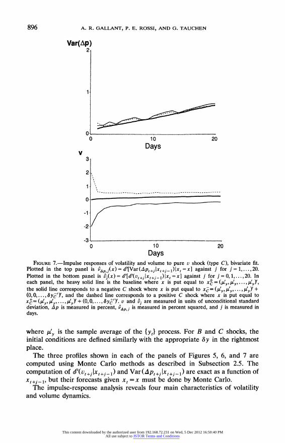
Days FIGURE 7.-Impulse responses of volatility and volume to pure v shock (type C), bivariate fit.

Plotted in the top panel is iP, i(x)= 4'[Var(A pt+jIxt+j-1) xt=x] against j for j=1,...,20. Plotted in the bottom panel is Q (x)= 4[4'(vt+jIxt+j1) Ix=xx] against j for j=0,1,...20. In each panel, the heavy solid line is the baseline where x is put equal to xo = (!,uy, W. Y y the solid line corresponds to a negative C shock where x is put equal to xc= (/yUSy, ..,A,SyY + (0?,0 -. 6 yE'Y, and the dashed line corresponds to a positive C shock where x is put equal to

=(Ii,, WYp9... tWY y+ (0,0... +'Y. v and Uj are measured in units of unconditional standard deviation, Ap is measured in percent, vp is measured in percent squared, and j is measured in days.

where 1iY is the sample average of the {yt) process. For B and C shocks, the initial conditions are defined similarly with the appropriate Sy in the rightmost place.

The three profiles shown in each of the panels of Figures 5, 6, and 7 are computed using Monte Carlo methods as described in Subsection 2.5. The computation of 64(vt+jlxt+j>1) and Var(Apt+jlxt+j-1) are exact as a function of xt+j-1, but their forecasts given xt = x must be done by Monte Carlo.

The impulse-response analysis reveals four main characteristics of volatility and volume dynamics.




First, asymmetry of the volatility response (the leverage effect) is attenuated and is essentially a transient effect in the bivariate system. This can be seen by comparing the top panels of Figures 5 and 6 to Figure 2 and noting that in Figures 5 and 6 the leverage effect damps in about five or six days. The damping of leverage is much more rapid than the slow damping of volatility back towards baseline.

Second, the impulse responses of volume to volume shocks (C shocks) are symmetric and extremely slowly damped, as can be seen in the bottom panel of Figure 7.

Third, volume shocks (C shocks)- have a very small effect on subsequent price volatility, as is evident in the top panel of Figure 7. This very mild feedback from volume to volatility is consistent with the findings of Schwert (1989) who applies linear methods to volume and a constructed volatility series. Weak feedback suggests that the price series is nearly Granger causally prior in the nonlinear sense discussed by Chamberlain (1982).

Fourth, large price movements to common-knowledge information events (B shocks) increase volume in the very short run but decrease volume over the longer term. This can be seen in the bottom panel of Figure 6. The short-run positive effect is evident in the work of Gallant, Rossi, and Tauchen (1992) who examine one-step ahead volatility. The very slowly damped long-term negative effect is a new finding of this paper.

The two most interesting and novel findings are the first, which pertains to long-term attenuation of leverage, and the fourth, which pertains to the contrast between the short- and long-term effects of price shocks on volume.

6. CONFIRMATION OF IMPULSE-RESPONSE RESULTS

6.1. Robustness to Conditioning Set

As previously noted in Section 3, there are two notions of a representative impulse-response sequence. The first, as just seen, is to use the unconditional mean of {xtj as the starting point: xo = (pZY' ... . , y'Y. The second is to average the impulse responses over the unconditional distribution of xt. Figure 8 shows impulse responses computed for the B-shock computed the latter way. The top panel pertains to price volatility, where the negative, baseline, and positive response sequences are computed as

1 16127

p,j 16100 EVAP,j(XT1+8X), ,r= 28

1 16127

VjPj = 16100 E VAP, j(X-1), ,r= 28

1 16127 EVAPJ(X 1+ax-),

16100 rr28

for j= 1, 2,9..., 20, where Ax+= (0,, .. ., y+')' and Ax =(0, 0, ..,y TY. For




Var(Ap) 4

3

2 -

0 10 20

v Days

0.2

0.0 -0.1 .A

-0.2 \,

-0.3

-0.4 0 10 20

Days FIGURE 8.-Impulse responses of volatility and volume to pure ap shock (type B), averaged over

the unconditional distribution of {xj}, bivariate fit. Plotted in the top panel is vP .=

(1/16100)E1,=284'[Var(Ap'+ Ix1+j1)Ix1 -T] against j for j-1, . .20. Plotted in the bottom

panel is Q =(1/16100)E )4'Xv1+1Ix+ xt=-)x1 ] against j for j=0,1,...,20. In each panel, the heavy solid line is the baseline where XT = xT, the solid line corresponds to a negative B shock where XfT = xT + (0, 0, ... ., SYB'Y, and the dashed line corresponds to a positive B shock where

XT- xT+ (0,o ...,SYB Y. x-1 = (APT-16,T-167 ...P1,vT-1). v and uj are measured in units of unconditional standard deviation, zp is measured in percent, PAP ] is measured in percent squared, and j is measured in days.

the bottom panel, the averaged impulse responses for the volume are 1 16127

V= 0 +a 16100 E ( 1 )

1 16127

= T16100 E (28 1 16127

16100 i 28




for j = 0, 1, 2,.. ., 20. As expected, the baselines in Figure 8 are flat. The lack of baseline drift is due to averaging over many baselines with different patterns of drift. Comparing Figure 8 to Figure 6 indicates that, for this data set, the patterns for B shocks relative to the baselines are robust to the method used to compute the representative response. The same is true for A and C shocks (figures not shown).

6.2. Contrasts with Linear Models

A reasonable question is whether our findings could have been uncovered by fitting a more traditional linear model. To address this issue, we computed the impulse-response sequences for the three types of shocks using a highly restricted SNP model. The restricted model has a linear specification for the conditional mean function coupled with an ARCH-type specification for the conditional variance function, each with a lag length of 16. The conditional second moment specification of the restricted SNP model differs only mildly from the ARCH model of Engle (1982) in that it parameterizes the conditional standard deviation instead of the conditional variance. The error density is a modified Hermite-expansion with quartic polynomial to capture the thick-tailed character of the distribution. To be precise, the fitted model is the 16 4 0 0 0 0 SNP specification reported in Table 5, p. 218, of Gallant, Rossi, and Tauchen (1992). The restricted SNP model is very close to the basic ARCH model with non-normal errors that has been utilized in many empirical finance studies (see Engle and Bollerslev (1986), and Engle and Gonzales-Rivera (1991)). Conven- tional model selection criteria and specification tests sharply reject this model in favor of more complicated SNP models, so it is interesting to investigate what features of the data it misses.

Figure 9 shows the impulse-response sequences for the B-shocks (common knowledge events) based on this specification of the conditional density. The sequences were computed using the second method which averages over all xt in the data set, so the figure is directly comparable to Figure 8.

In the top panel of Figure 9, the conditional variance responses to positive and negative shocks are constrained to be identical due to the symmetry of the basic ARCH specification. In contrast, the fully parameterized SNP fit used for Figure 8 displays damped asymmetry. Also, there is a noticeable baseline drift in the top panel of Figure 9 which is likely due to the misspecification intrinsic in this model.

The bottom panel of Figure 9 shows the volume responses to these positive and negative price shocks, which are constrained to be mirror images of one another due to the linear specification of the conditional mean function. This panel differs dramatically from its counterpart in Figure 8 obtained from the full SNP fit. In particular, the short-run increase in volume followed by a long-run decline for both positive and negative shocks is totally absent. The similar responses in volume irrespective of the sign of the price shock are to be expected, because of the well-known contemporaneous relationship between




Var(Ap) 4.

3

2

O.- 0 10 20

v Days 0.4-

0.3 ,,

0.2 - - - -

0.1.

0.0

-0.1

-0.2

-0.3

-0.4 0 10 20

Days FIGURE 9.-Impulse responses of volatility and volume to pure Ap shock (type B) from a linear

ARCH, averaged over the unconditional distribution of {xj), bivariate fit. Plotted in the top panel is Vdpj = (1/16 28,e[Var ( pt +j Ixt +j -)jXt = X_ 1 against j for j = 1, . 20. Plotted in the bottom panel is =(1/16100)E161274[4(vt+jxt+j_l)lXt=I_x -1] against j for j=0,1,...,20. In each panel, the heavy solid line is the baseline where x' = x7, the solid line corresponds to a negative B shock where A

r = x + (0,0 . . ., Y y'Y, and the dashed line corresponds to a positive B shock where x7=x +(0,0,... yB'Y. x7=(Apr166,vr716,.A-,p71 ,v7-1). v and Vj are measured in units of unconditional standard deviation, Ap is measured in percent, vjp j is measured in percent squared, and j is measured in days.

volume and the magnitude of the price change. The symmetries imposed by the linear specification result in misleading impressions of the dynamics.

6.3. Confidence Bands for Key Findings

The two main characteristics uncovered in Section 5 are attenuated damped leverage and the differential short- and long-term response of volume to price shocks. These characteristics, apparent from the point estimates, require statistical validation. Figures 10, 11, and 12 show 95 percent, sup-norm confidence



NONLINEAR DYNAMIC STRUCrURES 901

Var(Ap) 2

? o --

-1

-2 0 10 20

Days FIGURE 10.-95% confidence band for differential response of volatility to Ap and v shock (type

A), bivariate fit. The solid line is A A j= j jP(Xj4)- vp jx(x) plotted against j for j= 1.20

where Avp, j(x) = 4'[Var(Ap,+jIx, +j1)Ix, =x], x,= (/1y,, p.i . Y + (0,0. 8y,Y'Y, and x)+=

(/y,,Y, -..,y)' + (0,0..(SyA4'Y. The dashed lines show a constant width, simultaneously valid 95% confidence interval on the 20 values of APp,j. Ap is measured in percent, A A is measured in percent squared, and j is measured in days.

Var(Ap) 2

C2.

0 10 20 Days

FIGURE 11.-95% confidence band for differential response of volatility to Ap shock, univariate fit. The solid line is A

p,j= jA p,j(X+)_ A

J(X-) plotted against j for j = 1,..20 where VAP,j(X) = 4'[Var(Ap,+j1x,+j11)Ix, =X], X-= (/y yg .. WY)' + (0,0, ... . -5.0Y, and x+= (/4,,Ay9 ... .,) 'yy + (0,0 0 . . ., 5.0)'. The dashed lines show a constant width, simultaneously valid 95 % confidence interval on the 20 values of AA ij. Ap is measured in percent, AAp is measured in percent squared, and j is measured in days.




V

0.6

0.3

0.0 A%

-0.3\

-0.61 0 10 20

Days v 0.6

0.3

0.0

-0.3- - ' --- - - - -

-0.6 0 10 20

Days FIGURE 12.-95% confidence band for differential response of volume to pure Ap shock (type

B), bivariate fit. The solid line in the top panel is Q (x -) plotted against j for j = 0, 1, . . ., 20 where XB = (/i, tz t..,Y + (0, ?,..., 0 y -'Y. The dashed lines show a constant width, simultaneously valid 95% confidence interval on the values of Q (x-) for j = 1. 20. The solid line in the bottom panel is Dj(x ) plotted against j for j = 0,1,...,20 where B1(x) = 4'[4'(v,+jIx,+ j)Ix, =x] and x+= (/ty, y.../zY + (0,0...Sy'Y. The dashed lines show a constant width, simultaneously valid 95 % confidence interval on the values of b1(xB ) for j = 1, . 20. v and Vj(x) are measured in units of unconditional standard deviation and j is measured in days.

bands around quantities relevant for these findings, and thereby provide an indication of the statistical significance. We compute the bands for the first type of impulse-response functions where the unconditional mean of x, is the starting point. The computations for the bands are considerably less demanding for the first type and the robustness analysis suggested similar point estimates. The confidence bands are 95 percent sup-norm confidence bands obtained by bootstrapping as described in Subsection 2.6.

Figure 10 shows a 95 percent confidence band around the estimates

7A {+8 _7A PJX-) 1, 2= .. o 20




If the population volatility function is symmetric, that is, the leverage effect is absent, then the above differences should be jointly insignificant. The figure suggests some evidence for asymmetry in the first five days followed by no detectable asymmetry; the sup-norm bands after day five are tightly centered about zero differential response.

Figure 11 shows a 95 percent confidence band for the differential response of volatility from the univariate estimation discussed in Subsection 5.1 above. The point estimate of the differential response shows persistent asymmetry, though the confidence band is wide and includes zero for all but one day. Overall, our interpretation from the two figures is that there is some evidence for short-run asymmetry but very little evidence for long-term persistent asymmetry.

The top and bottom panels of Figure 12 show similarly constructed 95 percent confidence bands around the effects of pure price shocks on volume relative to baseline. The top panel shows

v;(Xs -(x0) ? m095 (j= 1, 2,....,20)

while the bottom panel shows

t;(X) -vx)J XB 9 (j= 1, 2,..., 20)

where the M's are computed as described in Subsection 2.6. The confidence bands indicate that the short-run increase in volume generated by the price shock is marginally statistically significant at the 95 percent level. On the other hand, the long-term decrease in volume is more strongly significant. The long-term decrease in volume presents a challenge to theoretical models of short-term speculative trading. Models based on either the notion of a random mixing process forcing a sequence of equilibria (Tauchen and Pitts (1983), Andersen (1992), Gallant and Tauchen (1992b)) or the notion of a market microstructure (Foster and Viswanathan (1992)) predict that volume remains above baseline.

7. PERSISTENCE IN VARIANCE

If a GARCH model is fitted to short-term financial price movements, then the implied volatility process looks integrated, or very nearly so (Engle and Bollerslev (1986)). Nelson (1990) presents theoretical evidence that one should expect to see a "unit-root" in variance as data are sampled more frequently, even if the true process is stationary. His findings are the second-moment analogues of Sims's (1984) findings regarding the martingale-like behavior of financial prices.

We utilize the methods of Subsection 2.7 to examine persistence properties of the price and volume process. The top panel of Figure 13 shows overplots of conditional mean profiles {APj(x)}J.1, for x E {xc : t = 28, 156, 284, ... 16028}. Some reduction of the 16,100 available x values is needed to keep the plots from becoming overly dense. The choice of every 128th xt, which generates 125 profiles, was determined by experimentation. The middle panel of Figure 13



904 A. R. GALLANT, P. E. ROSSI, AND G. TAUClHEN

(a)

C)

C\j

CMD

0 20 40 (b) 80 100

01

(b)

CIO

0 20 40 60 80 100 (C)

0 20 40 60 80 100 FIGURE 13.-Profiles, bivariate fit. Panel (a) shows overplots for T= 28,156,...,16028 of the

conditional mean profiles {Aj3(x,)})j'o where Aj(x)= [42(Ap,?+1x,?ji)1x1 =x,.l] Panel (b) shows overplots for r = 28,156,...,16028 of the conditional mean profiles {Qj(x,)}Ijlo where Q(x) = &[6(vt+jlx +j-l)Ixt =x1-l]. Panel (c) shows overplots for r = 28,156,...,16028 of the conditional volatility profiles {v(A j(xt))j.j where 'P, j(x) = 4'[Var (zip1 +j Ix+jx ) - X) Ixt = -1] against j for j 1. 20. v and Vj are measured in uinits of unconditional standard deviation, Ap is measured in percent, p 1 is measured in percent squared, and j is measured in days.

shows overplots of similarly constructed profiles for the volume. For each t, the profile is computed out J = 100 steps.

The profile for Ap shown in the top panel shows that this series is clearly not integrated; there is a very strong damping of the profiles to the unconditional mean. The volume series, however, shows a damping of the profiles consistent with stationarity but at a much slower rate than for the ap series. Examination of the plot shows a half rate of decay of the initial perturbation of some 40 periods. This is roughly consistent with the sort of damping expected in an AR(1) model with an autoregressive parameter of 0.90.

The bottom panel of Figure 13 shows the conditional volatility profiles {vAP,j(x)},1? for x E {x,: t = 28, 156,284,..., 16028} which is the same set of x's used in the conditional mean profiles. The volatility profiles suggest that shocks to variance are very slowly damped, but do die out. The volatility shows little evidence of integration 100 steps out. The profile for the bivariate fits contrast sharply with very unstable and persistent profiles for the univariate fitted SNP. For example, the univariate volatility profile shown in Figure 1 shows little evidence of convergence to the baseline. Recall from Subsection 3.2, that the conditional volatility profiles for an AR(1) model with GARCH(1, 1) errors will




damp at a geometric rate governed by a +,B: a5 [Var (Ajpt +j Ixt +j _ 1 ) Ixt I

j-1

E (a +I3)k + (8 + a)j-la(yt - Ayt-1) k=O

+ (,B + a) j 1,8 Var (Apt Ixt _ ). For an I-GARCH model, a + ,8 = 1, the profile for each xt is

69[Var (pt+jlxt+j-,)Ixt] = (-l1)a + a(y, Ayt_1)2

+ ,B Var (AptIxt1)

which shows linear drift away from a value that depends strongly on xt. The volatility profiles do not display this type of long-term dependence on initial condition characteristic of the I-GARCH model.

Some caution should be exercised in interpreting our findings on persistence. The Markovian structure of the SNP model allows for only a finite number of lags of the variables in the conditioning set. To capture extremely long-run persistence may require a very large number of lags. Diagnostics performed by Gallant, Rossi, and Tauchen (1992) suggest that the fitted bivariate SNP model fails to capture some of the movements of volatility at a yearly frequency; however, additional evidence shows that volatility computed from the fitted bivariate SNP closely conforms to movements in volatility on a monthly and shorter term basis.

8. CONCLUSION

We have developed an approach for analyzing the dynamics of a nonlinear time series that is represented by a nonparametric estimate of its one-step ahead conditional density. The approach entails examination of conditional moment profiles corresponding to certain shocks; a conditional moment profile is the conditional expectation evaluated at time t of a time invariant function evaluated at time t +i regarded as a function of j. The difference between a conditional moment profile and a baseline profile is the generalization of linear impulse-response analysis to the nonlinear situation. The approach includes strategies for laying out realistic perturbation experiments in multivariate situations and for undertaking statistical inference using bootstrap methods.

The empirical work uncovers two important new characteristics of the multi- period dynamics of the market price change and the transactions volume on the NYSE. First, the so-called leverage effect is a heavily damped transient phenomenon; it is both statistically and practically insignificant five to six days after a large movement in the market. Second, large price movements on common- knowledge information generate increased volume in the short run but reduce volume over the longer term.

The work underscores the importance of using nonlinear models to capture dynamics. In particular, the two major findings would have been missed com-




pletely by models linear in the conditional mean and/or variance functions. The work also demonstrates potential for using nonparametric density estimates to implement practicable inference procedures based on bootstrap methods.

Dept. of Statistics, North Carolina State University, Raleigh, NC 27695, U.S.A., Grad. School of Business, University of Chicago, 1101 E. 58th St., Chicago, IL

60637, U.SA. and

Dept. of Economics, Duke University, Durham, NC 27708, U.S.A.

Manuscript received November 1990; final revision received November, 1992.

REFERENCES

ANDERSEN, TORBEN (1992): "Return Volatility and Trading Volume in Financial Markets: An Information Interpretation of Stochastic Volatility," unpublished Ph.D. dissertation, Yale Uni- versity.

ANDREWS, DONALD W. K. (1991): "Asymptotic Normality of Series Estimators for Nonparametric and Semiparametric Models," Econometrica, 59, 307-346.

BICKEL, PETER J. (1992): "Theoretical Comparison of Different Bootstrap t Confidence Bounds," in Exploring the Limits of Bootstrap, ed. by Raoul LePage and Lynne Billard. New York: Wiley.

BLACK, F. (1976): "Studies of Stock Market Volatility Changes," Proceedings of the American Statistical Association, Business and Economics Section, 177-181.

BLANCHARD, OLIVIER J., AND DANNY QuAH (1989): "The Dynamic Effects of Aggregate Supply and Demand Disturbances," American Economic Review, 79, 655-673.

BLANCHARD, OLIVIER J., AND MARK W. WATSON (1986): "Are Business Cycles All Alike?" in The American Business Cycle: Continuity and Change, NBER Research Studies in Business Cycles, Vol. 25, ed. by R. J. Gordon. Chicago: University of Chicago Press.

BLUME, LAWRENCE, DAVID EASLEY, AND MAUREEN O'HARA (1991): "Market Statistics and Techni- cal Analysis: The Role of Volume," unpublished manuscript, Cornell University.

BOLLERSLEV, TIM (1986): "Generalized Autoregressive Conditional Heteroskedasticity," Journal of Econometrics, 31, 307-327.

BOLLERSLEV, TIM, RAY CHOU, AND KENNETH KRONER (1992): "ARCH Modeling in Finance: A Selective Review of the Theory and Empirical Evidence, with Suggestions for Future Research," Journal of Econometrics, 52, 5-61.

BOLLERSLEV, TIM, AND ROBERT ENGLE (1993): "Common Persistence in Conditional Variances," Econometrica, 61, 167-186.

CHAMBERLAIN, GARY (1982): "The General Equivalence of Granger and Sims Causality," Econo- metrica, 50, 569-582.

CHRISTIE, A. (1982): "The Stochastic Behavior of Common Stock Variances: Value, Leverage and Interest Rate Effects," Journal of Financial Economics, 10, 407-432.

DE LONG, J. BRADFORD, ANDREI SHLEIFER, LAWRENCE H. SUMMERS, AND ROBERT J. WALDMANN (1990): "Noise Trader Risk in Financial Markets," Journal of Political Economy, 98, 703-738.

DOAN, THOMAS, ROBERT LITTERMAN, AND CHRISTOPHER SIMS (1984): "Forecasting and Conditional Projection using Realistic Prior Distributions," Econometric Reviews, 3, 1-100.

EASTWOOD, BRIAN J. (1991): "Asymptotic Normality and Consistency of Semi-nonparametric Regression Estimators Using an Upward F Test Truncation Rule," Journal of Econometrics, 48, 151-182.

EFRON, BRADLEY (1992): "Six Questions Raised by the Bootstrap," in Exploring the Limits of Bootstrap, ed. by Raoul LePage and Lynne Billard. New York: Wiley.

EFRON, BRADLEY, AND RAOUL LEPAGE (1992): "Introduction to Bootstrap," in Exploring the Limits of Bootstrap, ed. by Raoul LePage and Lynne Billard. New York: Wiley.

ENGLE, ROBERT F. (1982): "Autoregressive Conditional Heteroskedasticity with Estimates of the Variance of United Kingdom Inflations," Econometrica, 50, 987-1008.




ENGLE, ROBERT F., AND TIM BOLLERSLEV (1986): "Modeling the Persistence of Conditional Variance," Econometric Reviews, 5, 1-50.

ENGLE, ROBERT F., AND GLORIA GONZALES-RIVERA (1991): "Semiparametric ARCH Models," Journal of Business and Economic Statistics, 9, 345-360.

ENGLE, ROBERT F., TAKATOSHI ITO, AND WEN-LING LIN (1990): "Meteor Showers or Heat Waves?" Heteroskedastic Intra-Daily Volatility in the Foreign Exchange Market," Econometrica, 58, 525-542.

FRENCH, K., G. W. SCHWERT, AND R. STAMBAUGH (1987): "Expected Stock Returns and Volatility," Journal of Financial Economics, 19, 3-30.

FOSTER, DOUGLAS, AND S. VISWANATHAN (1992): "Can Speculative Trading Explain the Volume- Volatility Relation?" unpublished manuscript, Fuqua School of Business, Duke University.

GALLANT, A. RONALD (1987): Nonlinear Statistical Models. New York: Wiley. GALLANT, A. RONALD, PETER E. ROSSI, AND GEORGE TAUCHEN (1992): "Stock Prices and Volume,"

Review of Financial Studies, 5, 199-242. GALLANT, A. RONALD, AND GERALDO SOUZA (1991): "On the Asymptotic Normality of Fourier

Flexible Form Estimates," Journal of Econometrics, 50, 329-353. GALLANT, A. RONALD, AND GEORGE TAUCHEN (1992a): "A Nonparametric Approach to Nonlinear

Time Series Analysis: Estimation and Simulation," in New Directions in Time Series Analysis, ed. by D. Brillinger, P. Caines, J. Geweke, E. Parzen, M. Rosenblatt, and M. Taqqu. New York: Springer-Verlag, pp. 71-92.

(1992b): "Which Moments to Match?" unpublished manuscript, Duke University. KARPOFF, J. (1987): "The Relation between Price Changes and Trading Volume: A Survey," Journal

of Financial and Quantitative Analysis, 22, 109-126. KING, ROBERT G., CHARLES I. PLOSSER, JAMES H. STOCK, AND MARK W. WATSON (1991):

"Stochastic Trends and Economic Fluctuations," American Economic Review, 81, 819-840. KYLE, ALBERT S. (1985): "Continuous Auctions and Insider Trading," Econometrica, 53, 1315-1336. LAMOUREUX, C., AND W. D. LASTRAPES (1992): "Endogenous Trading Volume and Momentum in

Stock Return Volatility," unpublished manuscript, Washington University in St. Louis. LANG, LARRY H. P., ROBERT H. LITZENBERGER, AND VINCENTE MADRIGAL (1992): "Testing

Financial Market Equilibrium under Asymmetric Information," Journal of Political Economy, 100, 317-348.

LIu, REGINA (1990): "On a Notion of Data Depth Based on Random Simplexes," Annals of Statistics, 18, 405-414.

Lo, ANDREW, AND A. MACKINLAY (1988): "Stock Market Prices Do Not Follow Random Walks: Evidence from a Simple Specification Test," Review of Financial Studies, 1, 41-66.

NELSON, DANIEL (1990): "Filtering and Forecasting with Misspecified ARCH Models I: Getting the Right Variance with the Wrong Model," unpublished manuscript, University of Chicago.

(1991): "Conditional Heteroskedasticity in Asset Returns: A New Approach," Econometrica, 59, 347-370.

NYCHKA, DOUGLAS, STEPHEN ELLNER, A. R. GALLANT, AND DANIEL MCCAFFREY (1992): "Finding Chaos in Noisy Systems," Journal of the Royal Statistical Society B, 54, 399-426.

POTTER, SIMON M. (1991): "Nonlinear Impulse-Response Functions," unpublished manuscript, University of California, Los Angeles.

ROBINSON, PETER M. (1983): "Nonparametric Estimators for Time Series," Journal of Time Series Analysis, 4, 185-207.

RUNKLE, DAVID E. (1987): "Vector Autoregressions and Reality," Journal of Business and Economic Statistics, 5, 437-442.

SCHWERT, G. WILLIAM (1989): "Why Does Stock Volatility Change Over Time?" Journal of Finance, 44, 1115-1154.

(1990): "Stock Volatility and the Crash of '87," Review of Financial Studies, 3, 77-102. SIMS, CHRISTOPHER (1980): "Macroeconomics and Reality," Econometrica, 48, 1-48.

(1984): "Martingale-like Behavior of Interest Rates and Prices," Discussion Paper No. 205, University of Minnesota.

TAUCHEN, GEORGE, AND MARK PITTS (1983): "The Price Variability-Volume Relationship on Speculative Markets," Econometrica, 51, 485-505.



nonlinear dynamic structures - duke universitypublic.econ.duke.edu/~get/wpapers/grt1993.pdf ·...

Documents