nonlinear dispersive equations: local and global analysis terence tao
TRANSCRIPT

Nonlinear dispersive equations: local and global
analysis
Terence Tao
Department of Mathematics, UCLA, Los Angeles, CA 90095
E-mail address : [email protected]
1991 Mathematics Subject Classification. Primary 35Q53, 35Q55, 35L15
The author is partly supported by a grant from the Packard foundation.

To Laura, for being so patient.

Contents
Preface ix
Chapter 1. Ordinary differential equations 11.1. General theory 21.2. Gronwall’s inequality 111.3. Bootstrap and continuity arguments 201.4. Noether’s theorem 261.5. Monotonicity formulae 351.6. Linear and semilinear equations 401.7. Completely integrable systems 49
Chapter 2. Constant coefficient linear dispersive equations 552.1. The Fourier transform 622.2. Fundamental solution 692.3. Dispersion and Strichartz estimates 732.4. Conservation laws for the Schrodinger equation 822.5. The wave equation stress-energy tensor 892.6. Xs,b spaces 97
Chapter 3. Semilinear dispersive equations 1093.1. On scaling and other symmetries 1143.2. What is a solution? 1203.3. Local existence theory 1293.4. Conservation laws and global existence 1433.5. Decay estimates 1533.6. Scattering theory 1623.7. Stability theory 1713.8. Illposedness results 1803.9. Almost conservation laws 186
Chapter 4. The Korteweg de Vries equation 1974.1. Existence theory 2024.2. Correction terms 2134.3. Symplectic non-squeezing 2184.4. The Benjamin-Ono equation and gauge transformations 223
Chapter 5. Energy-critical semilinear dispersive equations 2315.1. The energy-critical NLW 2335.2. Bubbles of energy concentration 2475.3. Local Morawetz and non-concentration of mass 2575.4. Minimal-energy blowup solutions 262
vii
viii CONTENTS
5.5. Global Morawetz and non-concentration of mass 271
Chapter 6. Wave maps 2776.1. Local theory 2886.2. Orthonormal frames and gauge transformations 2996.3. Wave map decay estimates 3106.4. Heat flow 320
Chapter A. Appendix: tools from harmonic analysis 329
Chapter B. Appendix: construction of ground states 347
Bibliography 363
Preface
Politics is for the present, but an equation is something for eternity.(Albert Einstein)
This monograph is based on (and greatly expanded from) a lecture series givenat the NSF-CBMS regional conference on nonlinear and dispersive wave equationsat New Mexico State University, held in June 2005. Its objective is to presentsome aspects of the global existence theory (and in particular, the regularity andscattering theory) for various nonlinear dispersive and wave equations, such as theKorteweg-de Vries (KdV), nonlinear Schrodinger, nonlinear wave, and wave mapsequations. The theory here is rich and vast and we cannot hope to present acomprehensive survey of the field here; our aim is instead to present a sample ofresults, and to give some idea of the motivation and general philosophy underlyingthe problems and results in the field, rather than to focus on the technical details.We intend this monograph to be an introduction to the field rather than an ad-vanced text; while we do include some very recent results, and we imbue some moreclassical results with a modern perspective, our main concern will be to developthe fundamental tools, concepts, and intuitions in as simple and as self-containeda matter as possible. This is also a pedagogical text rather than a reference; manydetails of arguments are left to exercises or to citations, or are sketched informally.Thus this text should be viewed as being complementary to the research literatureon these topics, rather than being a substitute for them.
The analysis of PDE is a beautiful subject, combining the rigour and techniqueof modern analysis and geometry with the very concrete real-world intuition ofphysics and other sciences. Unfortunately, in some presentations of the subject (atleast in pure mathematics), the former can obscure the latter, giving the impressionof a fearsomely technical and difficult field to work in. To try to combat this, thisbook is devoted in equal parts to rigour and to intuition; the usual formalism ofdefinitions, propositions, theorems, and proofs appear here, but will be interspersedand complemented with many informal discussions of the same material, centeringaround vague “Principles” and figures, appeal to physical intuition and examples,back-of-the-envelope computations, and even some whimsical quotations. Indeed,the exposition and exercises here reflect my personal philosophy that to truly under-stand a mathematical result one must view it from as many perspectives as possible(including both rigorous arguments and informal heuristics), and must also be ableto translate easily from one perspective to another. The reader should thus beaware of which statements in the text are rigorous, and which ones are heuristic,but this should be clear from context in most cases.
To restrict the field of study, we shall focus primarily on defocusing equations,in which soliton-type behaviour is prohibited. From the point of view of globalexistence, this is a substantially easier case to study than the focusing problem, in
ix
x PREFACE
which one has the fascinating theory of solitons and multi-solitons, as well as variousmechanisms to enforce blow-up of solutions in finite or infinite time. However, weshall see that there are still several analytical subtleties in the defocusing case,especially when considering critical nonlinearities, or when trying to establish asatisfactory scattering theory. We shall also work in very simple domains suchas Euclidean space Rn or tori Tn, thus avoiding consideration of boundary-valueproblems, or curved space, though these are certainly very important extensions tothe theory. One further restriction we shall make is to focus attention on the initialvalue problem when the initial data lies in a Sobolev space Hs
x(Rd), as opposed to
more localised choices of initial data (e.g. in weighted Sobolev spaces, or self-similarinitial data). This restriction, combined with the previous one, makes our choice ofproblem translation-invariant in space, which leads naturally to the deployment ofthe Fourier transform, which turns out to be a very powerful tool in our analysis.Finally, we shall focus primarily on only four equations: the semilinear Schrodingerequation, the semilinear wave equation, the Korteweg-de Vries equation, and thewave maps equation. These four equations are of course only a very small sample ofthe nonlinear dispersive equations studied in the literature, but they are reasonablyrepresentative in that they showcase many of the techniques used for more generalequations in a comparatively simple setting.
Each chapter of the monograph is devoted to a different class of differentialequations; generally speaking, in each chapter we first study the algebraic struc-ture of these equations (e.g. symmetries, conservation laws, and explicit solutions),and then turn to the analytic theory (e.g. existence and uniqueness, and asymptoticbehaviour). The first chapter is devoted entirely to ordinary differential equations(ODE). One can view partial differential equations (PDE) such as the nonlineardispersive and wave equations studied here, as infinite-dimensional analogues ofODE; thus finite-dimensional ODE can serve as a simplified model for understand-ing techniques and phenomena in PDE. In particular, basic PDE techniques suchas Picard and Duhamel iteration, energy methods, continuity or bootstrap argu-ments, conservation laws, near-conservation laws, and monotonicity formulae allhave useful ODE analogues. Furthermore, the analogy between classical mechan-ics and quantum mechanics provides a useful heuristic correspondence betweenSchrodinger type equations, and classical ODE involving one or more particles, atleast in the high-frequency regime.
The second chapter is devoted to the theory of the basic linear dispersive mod-els: the Airy equation, the free Schrodinger equation, and the free wave equation.In particular, we show how the Fourier transform and conservation law methods,can be used to establish existence of solutions, as well as basic estimates such asthe dispersive estimate, local smoothing estimates, Strichartz estimates, and Xs,b
estimates.In the third chapter we begin studying nonlinear dispersive equations in earnest,
beginning with two particularly simple semilinear models, namely the nonlinearSchrodinger equation (NLS) and nonlinear wave equation (NLW). Using theseequations as examples, we illustrate the basic approaches towards defining andconstructing solutions, and establishing local and global properties, though we de-fer the study of the more delicate energy-critical equations to a later chapter. (Themass-critical nonlinear Schrodinger equation is also of great interest, but we willnot discuss it in detail here.)

PREFACE xi
In the fourth chapter, we analyze the Korteweg de Vries equation (KdV), whichrequires some more delicate analysis due to the presence of derivatives in the non-linearity. To partly compensate for this, however, one now has the structures ofnonresonance and complete integrability; the interplay between the integrability onone hand, and the Fourier-analytic structure (such as nonresonance) on the other,is still only partly understood, however we are able to at least establish a quitesatisfactory local and global wellposedness theory, even at very low regularities,by combining methods from both. We also discuss a less dispersive cousin of theKdV equation, namely the Benjamin-Ono equation, which requires more nonlineartechniques, such as gauge transforms, in order to obtain a satisfactory existenceand wellposedness theory.
In the fifth chapter we return to the semilinear equations (NLS and NLW),and now establish large data global existence for these equations in the defocusing,energy-critical case. This requires the full power of the local wellposedness and per-turbation theory, together with Morawetz-type estimates to prevent various kindsof energy concentration. The situation is especially delicate for the Schrodingerequation, in which one must employ the induction on energy methods of Bourgainin order to obtain enough structural control on a putative minimal energy blowupsolution to obtain a contradiction and thus ensure global existence.
In the final chapter, we turn to the wave maps equation (WM), which is some-what more nonlinear than the preceding equations, but which on the other handenjoys a strongly geometric structure, which can in fact be used to renormalisemost of the nonlinearity. The small data theory here has recently been completed,but the large data theory has just begun; it appears however that the geometricrenormalisation provided by the harmonic map heat flow, together with a Morawetzestimate, can again establish global existence in the negatively curved case.
As a final disclaimer, this monograph is by no means intended to be a defini-tive, exhaustive, or balanced survey of the field. Somewhat unavoidably, the textfocuses on those techniques and results which the author is most familiar with, inparticular the use of the iteration method in various function spaces to establish alocal and perturbative theory, combined with frequency analysis, conservation laws,and monotonicity formulae to then obtain a global non-perturbative theory. Thereare other approaches to this subject, such as via compactness methods, nonlineargeometric optics, infinite-dimensional Hamiltonian dynamics, or the techniques ofcomplete integrability, which are also of major importance in the field (and cansometimes be combined, to good effect, with the methods discussed here); however,we will be unable to devote a full-length treatment of these methods in this text. Itshould also be emphasised that the methods, heuristics, principles and philosophygiven here are tailored for the goal of analyzing the Cauchy problem for semilineardispersive PDE; they do not necessarily extend well to other PDE questions (e.g.control theory or inverse problems), or to other classes of PDE (e.g. conservationlaws or to parabolic and elliptic equations), though there are certain many connec-tions and analogies between results in dispersive equations and in other classes ofPDE.
I am indebted to my fellow members of the “I-team” (Jim Colliander, MarkusKeel, Gigliola Staffilani, Hideo Takaoka), to Sergiu Klainerman, and to MichaelChrist for many entertaining mathematical discussions, which have generated muchof the intuition that I have tried to place into this monograph. I am also very
xii PREFACE
thankful for Jim Ralston for using this text to teach a joint PDE course, andproviding me with careful corrections and other feedback on the material. I alsothank Soonsik Kwon and Shaunglin Shao for additional corrections. Last, butnot least, I am grateful to my wife Laura for her support, and for pointing outthe analogy between the analysis of nonlinear PDE and the electrical engineeringproblem of controlling feedback, which has greatly influenced my perspective onthese problems (and has also inspired many of the diagrams in this text).
Terence Tao
Notation. As is common with any book attempting to survey a wide rangeof results by different authors from different fields, the selection of a unified no-tation becomes very painful, and some compromises are necessary. In this text Ihave (perhaps unwisely) decided to make the notation as globally consistent acrosschapters as possible, which means that any individual result presented here willlikely have a notation slightly different from the way it is usually presented in theliterature, and also that the notation is more finicky than a local notation wouldbe (often because of some ambiguity that needed to be clarified elsewhere in thetext). For the most part, changing from one convention to another is a matter ofpermuting various numerical constants such as 2, π, i, and −1; these constants areusually quite harmless (except for the sign −1), but one should nevertheless takecare in transporting an identity or formula in this book to another context in whichthe conventions are slightly different.
In this text, d will always denote the dimension of the ambient physical space,which will either be a Euclidean space1 Rd or the torus Td := (R/2πZ)d. (Chapter1 deals with ODE, which can be considered to be the case d = 0.) All integrals onthese spaces will be with respect to Lebesgue measure dx. If x = (x1, . . . , xd) andξ = (ξ1, . . . , ξd) lie in Rd, we use x · ξ to denote the dot product x · ξ := x1ξ1 + . . .+xdξd, and |x| to denote the magnitude |x| := (x2
1 + . . . + x2d)
1/2. We also use 〈x〉to denote the inhomogeneous magnitude (or Japanese bracket) 〈x〉 := (1 + |x|2)1/2of x, thus 〈x〉 is comparable to |x| for large x and comparable to 1 for small x.In a similar spirit, if x = (x1, . . . , xd) ∈ Td and k = (k1, . . . , kd) ∈ Zd we definek · x := k1x1 + . . .+ kdxd ∈ T. In particular the quantity eik·x is well-defined.
We say that I is a time interval if it is a connected subset of R which containsat least two points (so we allow time intervals to be open or closed, bounded orunbounded). If u : I×Rd → Cn is a (possibly vector-valued) function of spacetime,we write ∂tu for the time derivative ∂u
∂t , and ∂x1u, . . . , ∂xdu for the spatial derivatives
∂u∂x1
, . . . , ∂u∂xd; these derivatives will either be interpreted in the classical sense (when
u is smooth) or the distributional (weak) sense (when u is rough). We use ∇xu :I × Rd → Cnd to denote the spatial gradient ∇xu = (∂x1u, . . . , ∂xd
u). We caniterate this gradient to define higher derivatives ∇k
x for k = 0, 1, . . .. Of course,
1We will be using two slightly different notions of spacetime, namely Minkowski space R1+d
and Galilean spacetime R × Rd; in the very last section we also need to use parabolic spacetimeR+ × Rd. As vector spaces, they are of course equivalent to each other (and to the Euclidean
space Rd+1), but we will place different (pseudo)metric structures on them. Generally speaking,wave equations will use Minkowski space, whereas nonrelativistic equations such as Schrodingerequations will use Galilean spacetime, while heat equations use parabolic spacetime. For the mostpart the reader will be able to safely ignore these subtle distinctions.
PREFACE xiii
these definitions also apply to functions on Td, which can be identified with periodicfunctions on Rd.
We use the Einstein convention for summing indices, with Latin indices ranging
from 1 to d, thus for instance xj∂xju is short for∑d
j=1 xj∂xju. When we come
to wave equations, we will also be working in a Minkowski space R1+d with aMinkowski metric gαβ ; in such cases, we will use Greek indices and sum from 0 to d(with x0 = t being the time variable), and use the metric to raise and lower indices.Thus for instance if we use the standard Minkowski metric dg2 = −dt2 + |dx|2, then∂0u = ∂tu but ∂0u = −∂tu.
In this monograph we always adopt the convention that∫ ts
= −∫ st
if t < s.This convention will usually be applied only to integrals in the time variable.
We use the Lebesgue norms
‖f‖Lpx(Rd→C) := (
∫
Rd
|f(x)|p dx)1/p
for 1 ≤ p < ∞ for complex-valued measurable functions f : Rd → C, with theusual convention
‖f‖L∞x (Rd→C) := ess sup
x∈Rd
|f(x)|.
In many cases we shall abbreviate Lpx(Rd → C) as Lpx(R
d), Lp(Rd), or even Lp
when there is no chance of confusion. The subscript x, which denotes the dummyvariable, is of course redundant. However we will often retain it for clarity whendealing with PDE, since in that context one often needs to distinguish betweenLebesgue norms in space x, time t, spatial frequency ξ, or temporal frequencyτ . Also we will need it to clarify expressions such as ‖xf‖Lp
x(Rd), in which theexpression in the norm depends explicitly on the variable of integration. We ofcourse identify any two functions if they agree almost everywhere. One can ofcourse replace the domain Rd by the torus Td or the lattice Zd, thus for instance
‖f‖lpx(Zd→C) := (∑
k∈Zd
|f(k)|p)1/p.
One can replace C by any other Banach spaceX , thus for instance Lpx(Rd → X)
is the space of all measurable functions u : Rd → X with finite norm
‖u‖Lpx(Rd→X) := (
∫
Rd
‖u(x)‖pX dx)1/p
with the usual modification for p = ∞. In particular we can define the mixedLebesgue norms LqtL
rx(I ×Rd → C) = Lqt (I → Lrx(R
d → C)) for any time intervalI as the space of all functions u : I × Rd → C with norm
‖u‖LqtL
rx(I×Rd→C) := (
∫
I
‖u(t)‖qLr
x(Rd)dt)1/q = (
∫
I
(
∫
Rd
|u(t, x)|r dx)q/r dt)1/q
with the usual modifications when q = ∞ or r = ∞. One can also use this Banachspace notation to make sense of the Lp norms of tensors such as ∇f , ∇2f , etc.,provided of course that such derivatives exist in the Lp sense.
In a similar spirit, if I is a time interval and k ≥ 0, we use Ckt (I → X) todenote the space of all k-times continuously differentiable functions u : I → X with

xiv PREFACE
the norm
‖u‖Ckt (I→X) :=
k∑
j=0
‖∂jtu‖L∞t (I→X).
We adopt the convention that ‖u‖Ckt (I→X) = ∞ if u is not k-times continuously
differentiable. One can of course also define spatial analogues Ckx(Rd → X) of thesespaces, as well as spacetime versions Ckt,x(I×Rd → X). We caution that if I is notcompact, then it is possible for a function to be k-times continuously differentiablebut have infinite Ckt norm; in such cases we say that u ∈ Ckt,loc(I → X) rather than
u ∈ Ckt (I → X). More generally, a statement of the form u ∈ Xloc(Ω) on a domainΩ means that we can cover Ω by open sets V such that the restriction u|V of uto each of these sets V is in X(V ); under reasonable assumptions on X , this alsoimplies that u|K ∈ X(K) for any compact subset K of Ω. As a rule of thumb, theglobal spaces X(Ω) will be used for quantitative control (estimates), whereas thelocal spaces Xloc(Ω) are used for qualitative control (regularity); indeed, the localspaces Xloc are typically only Frechet spaces rather than Banach spaces. We willneed both types of control in this text, as one typically needs qualitative control toensure that the quantitative arguments are rigorous.
If (X, dX) is a metric space and Y is a Banach space, we use C0,1(X → Y ) todenote the space of all Lipschitz continuous functions f : X → Y , with norm
‖f‖C0,1(X→Y ) := supx,x′∈X:x 6=x′
‖f(x) − f(x′)‖YdX(x, x′)
.
(One can also define the inhomogeneous Lipschitz norm ‖f‖C0,1 := ‖f‖C0,1+‖f‖C0,
but we will not need this here.) Thus for instance C1(Rd → Rm) is a subset
of C0,1(Rd → Rm), which is in turn a subset of C0loc(R
d → Rm). The space
C0,1loc (X → Y ) is thus the space of locally Lipschitz functions (i.e. every x ∈ X is
contained in a neighbourhood on which the function is Lipschitz).In addition to the above function spaces, we shall also use Sobolev spaces Hs,
W s,p, Hs, W s,p, which are defined in Appendix A, and Xs,b spaces, which aredefined in Section 2.6.
If V andW are finite-dimensional vector spaces, we use End(V →W ) to denotethe space of linear transformations from V to W , and End(V ) = End(V → V ) forthe ring of linear transformations from V to itself. This ring contains the identitytransformation id = idV .
IfX and Y are two quantities (typically non-negative), we useX . Y or Y & Xto denote the statement that X ≤ CY for some absolute constant C > 0. We useX = O(Y ) synonymously with |X | . Y . More generally, given some parametersa1, . . . , ak, we use X .a1,...,ak
Y or Y &a1,...,akX to denote the statement that
X ≤ Ca1,...,akY for some (typically large) constant Ca1,...,ak
> 0 which can dependon the parameters a1, . . . , ak, and defineX = Oa1,...,ak
(Y ) similarly. Typical choicesof parameters include the dimension d, the regularity s, and the exponent p. Wewill also say that X is controlled by a1, . . . , ak if X = Oa1,...,ak
(1). We use X ∼Y to denote the statement X . Y . X , and similarly X ∼a1,...,ak
Y denotesX .a1,...,ak
Y .a1,...,akX . We will occasionally use the notation X ≪a1,...,ak
Yor Y ≫a1,...,ak
X to denote the statement X ≤ ca1,...,akY for some suitably small
quantity ca1,...,ak> 0 depending on the parameters a1, . . . , ak. This notation is

PREFACE xv
somewhat imprecise (as one has to specify what “suitably small” means) and so weshall usually only use it in informal discussions.
Recall that a function f : Rd → C is said to be rapidly decreasing if we have
‖〈x〉Nf(x)‖L∞x (Rd) <∞
for all N ≥ 0. We then say that a function is Schwartz if it is smooth and all of itsderivatives ∂αx f are rapidly decreasing, where α = (α1, . . . , αd) ∈ Zd+ ranges overall multi-indices, and ∂αx is the differential operator
∂αx := (∂
∂x1)α1 . . . (
∂
∂xd)αd .
In other words, f is Schwartz if and only if ∂αx f(x) = Of,α,N (〈x〉−N ) for all α ∈ Zd+and all N . We use Sx(Rd) to denote the space of all Schwartz functions. Asis well known, this is a Frechet space, and thus has a dual Sx(Rd)∗, the spaceof tempered distributions. This space contains all locally integrable functions ofpolynomial growth, and is also closed under differentiation, multiplication withfunctions g of symbol type (i.e. g and all its derivatives are of polynomial growth)and convolution with Schwartz functions; we will not present a detailed descriptionof the distributional calculus here.

CHAPTER 1
Ordinary differential equations
Science is a differential equation. Religion is a boundary condition.(Alan Turing, quoted in J.D. Barrow, “Theories of everything”)
This monograph is primarily concerned with the global Cauchy problem (orinitial value problem) for partial differential equations (PDE), but in order to as-semble some intuition on the behaviour of such equations, and on the power andlimitations of the various techniques available to analyze these equations, we shallfirst study these phenomena and methods in the much simpler context of ordinarydifferential equations (ODE), in which many of the technicalities in the PDE anal-ysis are not present. Conversely, the theory of ODEs, particularly HamiltonianODEs, has a very rich and well-developed structure, the extension of which to non-linear dispersive PDEs is still far from complete. For instance, phenomena fromHamiltonian dynamics such as Kolmogorov-Arnold-Moser (KAM) invariant tori,symplectic non-squeezing, Gibbs and other invariant measures, or Arnold diffusionare well established in the ODE setting, but the rigorous theory of such phenomenafor PDEs is still its infancy.
One technical advantage of ODE, as compared with PDE, is that with ODEone can often work entirely in the category of classical (i.e. smooth) solutions,thus bypassing the need for the theory of distributions, weak limits, and so forth.However, even with ODE it is possible to exhibit blowup in finite time, and in high-dimensional ODE (which begin to approximate PDE in the infinite dimensionallimit) it is possible to have the solution stay bounded in one norm but becomeextremely large in another norm. Indeed, the quantitative study of expressionssuch as mass, energy, momentum, etc. is almost as rich in the ODE world as it isin the PDE world, and thus the ODE model does serve to illuminate many of thephenomena that we wish to study for PDE.
A common theme in both nonlinear ODE and nonlinear PDE is that of feedback- the solution to the equation at any given time generates some forcing term, whichin turn feeds back into the system to influence the solution at later times, usuallyin a nonlinear fashion. The tools we will develop here to maintain control of thisfeedback effect - the Picard iteration method, Gronwall’s inequality, the bootstrapprinciple, conservation laws, monotonicity formulae, and Duhamel’s formula - willform the fundamental tools we will need to analyze nonlinear PDE in later chapters.Indeed, the need to deal with such feedback gives rise to a certain “nonlinear wayof thinking”, in which one continually tries to control the solution in terms of itself,or derive properties of the solution from (slightly weaker versions of) themselves.This way of thinking may initially seem rather unintuitive, even circular, in nature,but it can be made rigorous, and is absolutely essential to proceed in this theory.
1
2 1. ORDINARY DIFFERENTIAL EQUATIONS
1.1. General theory
It is a capital mistake to theorise before one has data. Insensiblyone begins to twist facts to suit theories, instead of theories to suitfacts. (Sir Arthur Conan Doyle, “A Study in Scarlet”)
In this section we introduce the concept of an ordinary differential equationand the associated Cauchy problem, but then quickly specialise to an importantsubclass of such problems, namely the Cauchy problem (1.7) for autonomous first-order quasilinear systems.
Throughout this chapter, D will denote a (real or complex) finite dimensionalvector space, which at times we will endow with some norm ‖‖D; the letter D standsfor “data”. An ordinary differential equation (ODE) is an equation which governscertain functions u : I → D mapping a (possibly infinite) time interval I ⊆ R tothe vector space1 D. In this setup, the most general form of an ODE is that of afully nonlinear ODE
(1.1) G(u(t), ∂tu(t), . . . , ∂kt u(t), t) = 0
where k ≥ 1 is an integer, and G : Dk+1×I → X is a given function taking values inanother finite-dimensional vector space X . We say that a function u ∈ Ckloc(I → D)is a classical solution2 (or solution for short) of the ODE if (1.1) holds for all t ∈ I.The integer k is called the order of the ODE, thus for instance if k = 2 then wehave a second-order ODE. One can think of u(t) as describing the state of somephysical system at a given time t; the dimension of D then measures the degreesof freedom available. We shall refer to D as the state space, and sometimes referto the ODE as the equation(s) of motion, where the plural reflects the fact that Xmay have more than one dimension. While we will occasionally consider the scalarcase, when D is just the real line R or the complex plane C, we will usually bemore interested in the case when the dimension of D is large. Indeed one can viewPDE as a limiting case of ODE as dim(D) → ∞.
In this monograph we will primarily consider those ODE which are time-translation-invariant (or autonomous), in the sense that the function G does notactually depend explicitly on the time parameter t, thus simplifying (1.1) to
(1.2) G(u(t), ∂tu(t), . . . , ∂kt u(t)) = 0
for some function G : Dk+1 → X . One can in fact convert any ODE into a time-translation-invariant ODE, by the trick of embedding the time variable itself intothe state space, thus replacing D with D ×R, X with X ×R, u with the function
1One could generalise the concept of ODE further, by allowing D to be a smooth manifoldinstead of a vector space, or even a smooth bundle over the time interval I. This leads for instanceto the theory of jet bundles, which we will not pursue here. In practice, one can descend from thismore general setup back to the original framework of finite-dimensional vector spaces - locallyin time, at least - by choosing appropriate local coordinate charts, though often the choice ofsuch charts is somewhat artifical and makes the equations messier; see Chapter 6 for some relatedissues.
2We will discuss non-classical solutions shortly. As it turns out, for finite-dimensional ODEthere is essentially no distinction between a classical and non-classical solution, but for PDE therewill be a need to distinguish between classical, strong, and weak solutions. See Section 3.2 forfurther discussion.

1.1. GENERAL THEORY 3
u(t) := (u(t), t), and G with the function3
G((u0, s0), (u1, s1), . . . , (uk, sk)) := (G(u0, . . . , uk), s1 − 1).
For instance, solutions to the non-autonomous ODE
∂tu(t) = F (t, u(t))
are equivalent to solutions to the system of autonomous ODE
∂tu(t) = F (s(t), u(t)); ∂ts(t) − 1 = 0
provided that we also impose a new initial condition s(0) = 0. This trick is notalways without cost; for instance, it will convert a non-autonomous linear equationinto an autonomous nonlinear equation.
By working with time translation invariant equations we obtain our first sym-metry, namely the time translation symmetry
(1.3) u(t) 7→ u(t− t0).
More precisely, if u : I → D solves the equation (1.2), and t0 ∈ R is any timeshift parameter, then the time-translated function ut0 : I + t0 → D defined byut0(t) := u(t − t0), where I + t0 := t + t0 : t ∈ I is the time translation of I,is also a solution to (1.2). This symmetry tells us, for instance, that the initialvalue problem for this equation starting from time t = 0 will be identical (afterapplying the symmetry (1.3)) to the initial value problem starting from any othertime t = t0.
The equation (1.2) implicitly determines the value of the top-order derivative
∂kt u(t) in terms of the lower order derivatives u(t), ∂tu(t), . . . , ∂k−1t u(t). If the
hypotheses of the implicit function theorem4 are satisfied, then we can solve for∂kt u(t) uniquely, and rewrite the ODE as an autonomous quasilinear ODE of orderk
(1.4) ∂kt u(t) = F (u(t), ∂tu(t), . . . , ∂k−1t u(t)),
for some function F : Dk → D. Of course, there are times when the implicitfunction theorem is not available, for instance if the domain Y of G has a differentdimension than that of D. If Y has larger dimension than D then the equation isoften over-determined ; it has more equations of motion than degrees of freedom,and one may require some additional hypotheses on the initial data before a solutionis guaranteed. If Y has smaller dimension than D then the equation is often under-determined ; it has too few equations of motion, and one now expects to have amultiplicity of solutions for any given initial datum. And even if D and Y havethe same dimension, it is possible for the ODE to sometimes be degenerate, in thatthe Jacobian that one needs to invert for the implicit function theorem becomessingular.
3Informally, what one has done is added a “clock” s to the system, which evolves at the fixedrate of one time unit per time unit ( ds
dt−1 = 0), and then the remaining components of the system
are now driven by clock time rather than by the system time. The astute reader will note that thisnew ODE not only contains all the solutions to the old ODE, but also contains some additionalsolutions; however these new solutions are simply time translations of the solutions coming fromthe original ODE.
4An alternate approach is to differentiate (1.2) in time using the chain rule, obtaining an
equation which is linear in ∂k+1t u(t), and provided that a certain matrix is invertible, one can
rewrite this in the form (1.4) but with k replaced by k + 1.
4 1. ORDINARY DIFFERENTIAL EQUATIONS
Degenerate ODE are rather difficult to study and will not be addressed here.Both under-determined and over-determined equations cause difficulties for analy-sis, which are resolved in different ways. An over-determined equation can often bemade determined by “forgetting” some of the constraints present in (1.2), for in-stance by projecting Y down to a lower-dimensional space. In many cases, one canthen recover the forgotten constraints by using some additional hypothesis on theinitial datum, together with an additional argument (typically involving Gronwall’sinequality); see for instance Exercises 1.13, (6.4). Meanwhile, an under-determinedequation often enjoys a large group of “gauge symmetries” which help “explain”the multiplicity of solutions to the equation; in such a case one can often fix a spe-cial gauge, thus adding additional equations to the system, to make the equationdetermined again; see for instance Section 6.2 below. In some cases, an ODE cancontain both over-determined and under-determined components, requiring one toperform both of these types of tricks in order to recover a determined equation,such as one of the form (1.4).
Suppose that u is a classical solution to the quasilinear ODE (1.4), and thatthe nonlinearity F : Dk → D is smooth. Then one can differentiate (1.4) in time,use the chain rule, and then substitute in (1.4) again, obtain an equation of theform
∂k+1t u(t) = Fk+1(u(t), ∂tu(t), . . . , ∂
k−1t u(t))
for some smooth function Fk+1 : Dk → D which can be written explicitly in termsof G. More generally, by an easy induction we obtain equations of the form
(1.5) ∂k′
t u(t) = Fk′ (u(t), ∂tu(t), . . . , ∂k−1t u(t))
for any k′ ≥ k, where Fk′ : Dk → D is a smooth function which depends only on Gand k′. Thus, if one specifies the initial data u(t0), . . . , ∂
k−1t u(t0) at some fixed time
t0, then all higher derivatives of u at t0 are also completely specified. This shows inparticular that if u is k− 1-times continuously differentiable and F is smooth, thenu is automatically smooth. If u is not only smooth but analytic, then from Taylorexpansion we see that u is now fixed uniquely. Of course, it is only reasonable toexpect u to be analytic if F is also analytic. In such a case, we can complementthe above uniqueness statement with a (local) existence result:
Theorem 1.1 (Cauchy-Kowalevski theorem). Let k ≥ 1. Suppose F : Dk → Dis real analytic, let t0 ∈ R, and let u0, . . . , uk−1 ∈ D be arbitrary. Then there existsan open time interval I containing t0, and a unique real analytic solution u : I → Dto (1.4), which obeys the initial value conditions
u(t0) = u0; ∂tu(t0) = u1, . . . , ∂k−1t u(t0) = uk−1.
We defer the proof of this theorem to Exercise 1.1. This beautiful theoremcan be considered as a complete local existence theorem for the ODE (1.4), inthe case when G is real analytic; it says that the initial position u(t0), and the
first k − 1 derivatives, ∂tu(t0), . . . , ∂k−1t u(t0), are precisely the right amount of
initial data5 needed in order to have a wellposed initial value problem (we willdefine wellposedness more precisely later). However, it turns out to have somewhat
5Conventions differ on when to use the singular “datum” and the plural “data”. In this text,we shall use the singular “datum” for ODE and PDE that are first-order in time, and the plural“data” for ODE and PDE that are higher order (or unspecified order) in time. Of course, in bothcases we use the plural when considering an ensemble or class of data.

1.1. GENERAL THEORY 5
limited application when we move from ODE to PDE (though see Exercise 3.25).We will thus rely instead primarily on a variant of the Cauchy-Kowalevski theorem,namely the Picard existence theorem, which we shall discuss below.
Remark 1.2. The fact that the solution u is restricted to lie in a open intervalI, as opposed to the entire real line R, is necessary. A basic example is the initialvalue problem
(1.6) ut = u2; u(0) = 1
where u takes values on the real line R. One can easily verify that the functionu(t) := 1
1−t solves this ODE with the given initial datum as long as t < 1, and thusis the unique real-analytic solution to this ODE in this region. But this solutionclearly blows up (i.e. ceases to be smooth) at t = 1, and so cannot be continued6
real analytically beyond this point.
There is a simple trick available to reduce a kth order ODE such as (1.4) to afirst order ODE, at the cost of multiplying the number of degrees of freedom by k,or more precisely, replacing the state space D by the phase space Dk. Indeed, ifone defines the new function u : I → Dk by
u(t) := (u(t), ∂tu(t), . . . , ∂k−1t u(t)),
then the equation (1.4) is equivalent to
∂tu(t) = F (u(t))
where F : Dk → Dk is the function
F (u0, . . . , uk−1) = (u1, . . . , uk−1, F (u0, . . . , uk−1)).
Furthermore, u is continuously differentiable if and only if u is k times continuouslydifferentiable, and the k initial conditions
u(t0) = u0; ∂tu(t0) = u1; . . . ; ∂k−1t u(t0) = uk−1
collapse to a single initial condition
u(t0) = u0 := (u0, . . . , uk−1).
Thus for the remainder of this chapter, we shall focus primarily on the initial valueproblem (or Cauchy problem) of obtaining solutions u(t) to the first-order ODE7
(1.7) ∂tu(t) = F (u(t)) for all t ∈ I; u(t0) = u0.
where the interval I, the initial time t0, the initial datum u0 ∈ D, and the nonlin-earity F : D → D are given. We will distinguish three types of solutions:
6One can of course consider a meromorphic continuation beyond t = 1, but this would requirecomplexifying time, which is a somewhat non-physical operation. Also, this complexification nowrelies very heavily on the analyticity of the situation, and when one goes from ODE to PDE, it isunlikely to work for non-analytic initial data. The question of whether one can continue a solutionin some weakened sense beyond a singularity is an interesting and difficult one, but we will notpursue it in this text.
7One can interpret F as a vector field on the state space D, in which case the ODE is simplyintegrating this vector field; see Figure 1. This viewpoint is particularly useful when consideringthe Hamiltonian structure of the ODE as in Section 1.4, however it is not as effective a conceptualframework when one passes to PDE.

6 1. ORDINARY DIFFERENTIAL EQUATIONS
u0
u(t)
F(u(t))
Figure 1. Depicting F as a vector field on D, the trajectory ofthe solution u(t) to the first order ODE (1.7) thus “follows thearrows” and integrates the vector field F . Contrast this “classi-cal solution” interpretation of an ODE with the rather different“strong solution” interpretation in Figure 2.
• A classical solution of (1.7) is a function u ∈ C1loc(I → D) which solves
(1.7) for all t ∈ I in the classical sense (i.e. using the classical notion ofderivative).
• A strong solution of (1.7) is a function u ∈ C0loc(I → D) which solves (1.7)
in the integral sense that
(1.8) u(t) = u0 +
∫ t
t0
F (u(s)) ds
holds for all8 t ∈ I;• A weak solution of (1.7) is a function u ∈ L∞(I → D) which solves (1.8)
in the sense of distributions, thus for any test function ψ ∈ C∞0 (I), one
has ∫
I
u(t)ψ(t) dt = u0
∫
I
ψ(t) +
∫
I
ψ(t)
∫ t
t0
F (u(s)) dsdt.
Later, when we turn our attention to PDE, these three notions of solutionshall become somewhat distinct; see Section 3.2. In the ODE case, however, wefortunately have the following equivalence (under a very mild assumption on F ):
Lemma 1.3. Let F ∈ C0loc(D → D). Then the notions of classical solution,
strong solution, and weak solution are equivalent.
Proof. It is clear that a classical solution is strong (by the fundamental the-orem of calculus), and that a strong solution is weak. If u is a weak solution, then
8Recall that we are adopting the convention thatR ts = −
R st if t < s.

1.1. GENERAL THEORY 7
Forcing termF(u)
Solutionuu
0Constant evolution
Integrationin time
Initial datum
Nonlinearity F
Figure 2. A schematic depiction of the relationship between theinitial datum u0, the solution u(t), and the nonlinearity F (u). Themain issue is to control the “feedback loop” in which the solutioninfluences the nonlinearity, which in turn returns to influence thesolution.
it is bounded and measurable, hence F (u) is also bounded and measurable. Thus
the integral∫ tt0F (u(s)) ds is Lipschitz continuous, and (since u solves (1.8) in the
sense of distributions) u(t) is also Lipschitz continuous, so it is a strong solution(we allow ourselves the ability to modify u on a set of measure zero). Then F (u)is continuous, and so the fundamental theorem of calculus and (1.8) again, u is infact in C1
loc and is a classical solution.
The three perspectives of classical, strong, and weak solutions are all importantin the theory of ODE and PDE. The classical solution concept, based on the differ-ential equation (1.7), is particularly useful for obtaining conservation laws (Section1.4) and monotonicity formulae (Section 1.5), and for understanding symmetriesof the equation. The strong solution concept, based on the integral equation (1.8),is more useful for constructing solutions (in part because it requires less a prioriregularity on the solution), and establishing regularity and growth estimates on thesolution. It also leads to a very important perspective on the equation, viewingthe solution u(t) as being the combination of two influences, one coming from theinitial datum u0 and the other coming from the forcing term F (u); see Figure 2.Finally, the concept of a weak solution arises naturally when constructing solutionsvia compactness methods (e.g. by considering weak limits of classical solutions),since continuity is not a priori preserved by weak limits.
To illustrate the strong solution concept, we can obtain the first fundamentaltheorem concerning such Cauchy problems, namely the Picard existence theorem.We begin with a simplified version of this theorem to illustrate the main point.
Theorem 1.4 (Picard existence theorem, simplified version). Let D be a finite-
dimensional normed vector space. Let F ∈ C0,1(D → D) be a Lipschitz function onD with Lipschitz constant ‖F‖C0,1 = M . Let 0 < T < 1/M . Then for any t0 ∈ R
and u0 ∈ D, there exists a strong (hence classical) solution u : I → D to the Cauchyproblem (1.7), where I is the compact time interval I := [t0 − T, t0 + T ].
8 1. ORDINARY DIFFERENTIAL EQUATIONS
Proof. Fix u0 ∈ D and t0 ∈ R, and let Φ : C0(I → D) → C0(I → D) be themap
Φ(u)(t) := u0 +
∫ t
t0
F (u(t′)) dt′.
Observe from (1.8) that a strong solution is nothing more than a fixed point of themap Φ. It is easy to verify that Φ is indeed a map from C0(I → D) to C0(I → D).Using the Lipschitz hypothesis on F and the triangle inequality, we obtain
‖Φ(u)(t) − Φ(v)(t)‖D = ‖∫ t
t0
F (u(t′)) − F (v(t′)) dt′‖D ≤∫ t
t0
M‖u(t′) − v(t′)‖D dt′
for all t ∈ I and u, v ∈ C0(I → Ωε), and thus
‖Φ(u) − Φ(v)‖C0(I→D) ≤ TM‖u− v‖C0(I→D).
Since we have TM < 1, we see that Φ will be a strict contraction on the completemetric space C0(I → D). Applying the contraction mapping theorem (Exercise 1.2)we obtain a fixed point to Φ, which gives the desired strong (and hence classical)solution to the equation (1.7).
Remark 1.5. An inspection of the proof of the contraction mapping theoremreveals that the above argument in fact gives rise to an explicit iteration schemethat will converge to the solution u. Indeed, one can start with the constantsolution u(0)(t) := u0, and then define further iterates u(n) ∈ C0(I → Ωε) byu(n) := Φ(u(n−1)), or in other words
u(n)(t) := u0 +
∫ t
t0
F (u(n−1)(t′) dt′.
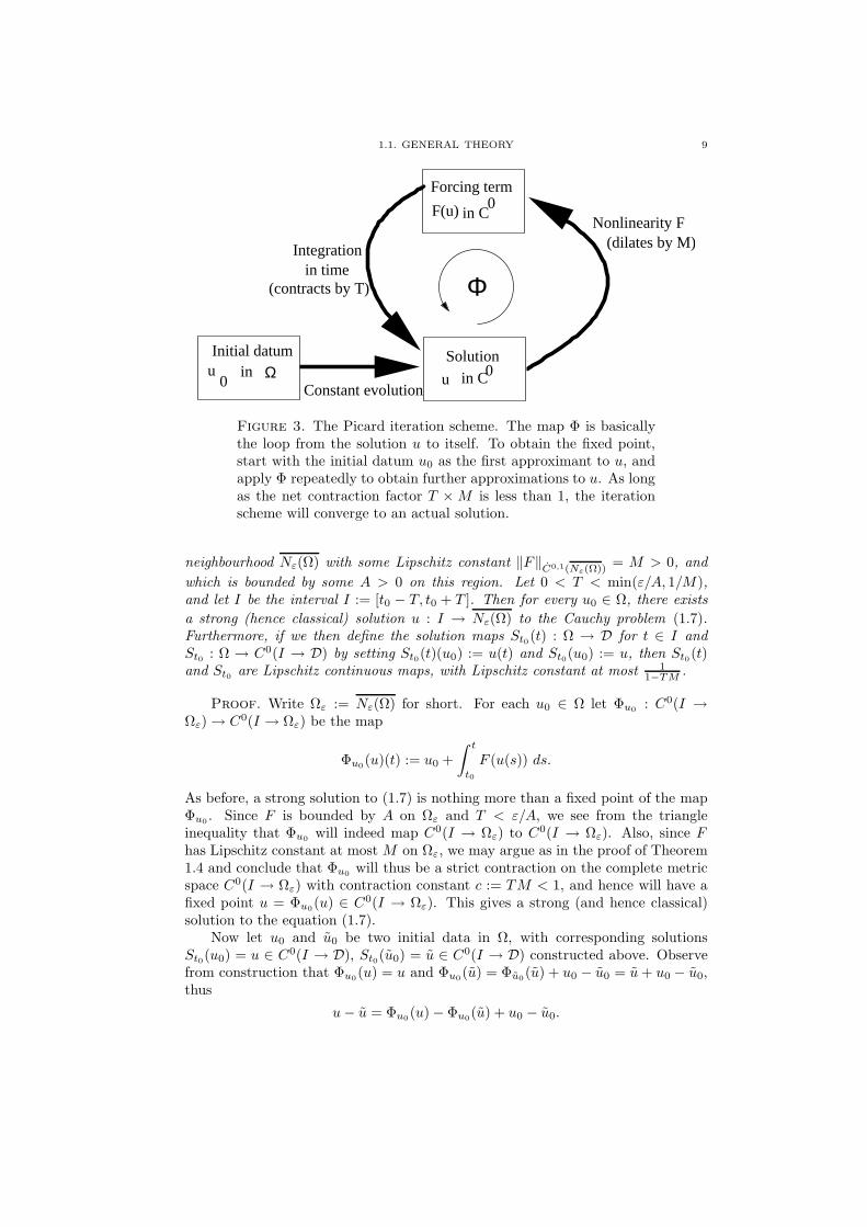
These Picard iterates do not actually solve the equation (1.7) in any of the abovesenses, but they do converge uniformly on I to the actual solution. See Figure 3.
Remark 1.6. The above argument is perhaps the simplest example of theiteration method (also known as the contraction mapping principle method or theinverse function theorem method), constructing a nonlinear solution as the stronglimit of an iterative procedure. This type of method will be our primary meansof generating solutions which obey a satisfactory set of existence, uniqueness, andregularity properties. Note that one needs to select a norm ‖‖D in order to obtaina quantitative estimate on the time of existence. For finite-dimensional ODE, theexact choice of norm is not terribly important (as all norms are equivalent), butselecting the norm in which to apply the contraction mapping theorem will becomedecisive when studying PDE.
Because F is assumed to be globally Lipschitz (C0,1), one can actually constructa global solution to (1.7) in this case, by iterating the above theorem; see Exercise
1.10. However, in most applications F will only be locally Lipschitz (C0,1loc ), and
so we shall need a more general version of the above existence theorem. Onesuch version (which also gives some further information, namely some Lipschitzcontinuity properties on the solution map) is as follows.
Theorem 1.7 (Picard existence theorem, full version). Let D be a finite-dimensional normed vector space. Let t0 ∈ R, let Ω be a non-empty subset of D,and let Nε(Ω) := u ∈ D : ‖u − v‖D < ε for some v ∈ Ω be the ε-neighbourhoodof Ω for some ε > 0. Let F : D → D be a function which is Lipschitz on the closed
1.1. GENERAL THEORY 9
Φ
Forcing term
Solution
Nonlinearity F
Constant evolution
Integrationin time
Ωin0
u
(dilates by M)
(contracts by T)
F(u) in C
in Cu 0
0
Initial datum
Figure 3. The Picard iteration scheme. The map Φ is basicallythe loop from the solution u to itself. To obtain the fixed point,start with the initial datum u0 as the first approximant to u, andapply Φ repeatedly to obtain further approximations to u. As longas the net contraction factor T ×M is less than 1, the iterationscheme will converge to an actual solution.
neighbourhood Nε(Ω) with some Lipschitz constant ‖F‖C0,1(Nε(Ω)) = M > 0, and
which is bounded by some A > 0 on this region. Let 0 < T < min(ε/A, 1/M),and let I be the interval I := [t0 − T, t0 + T ]. Then for every u0 ∈ Ω, there exists
a strong (hence classical) solution u : I → Nε(Ω) to the Cauchy problem (1.7).Furthermore, if we then define the solution maps St0(t) : Ω → D for t ∈ I andSt0 : Ω → C0(I → D) by setting St0(t)(u0) := u(t) and St0(u0) := u, then St0(t)and St0 are Lipschitz continuous maps, with Lipschitz constant at most 1
1−TM .
Proof. Write Ωε := Nε(Ω) for short. For each u0 ∈ Ω let Φu0 : C0(I →Ωε) → C0(I → Ωε) be the map
Φu0(u)(t) := u0 +
∫ t
t0
F (u(s)) ds.
As before, a strong solution to (1.7) is nothing more than a fixed point of the mapΦu0 . Since F is bounded by A on Ωε and T < ε/A, we see from the triangleinequality that Φu0 will indeed map C0(I → Ωε) to C0(I → Ωε). Also, since Fhas Lipschitz constant at most M on Ωε, we may argue as in the proof of Theorem1.4 and conclude that Φu0 will thus be a strict contraction on the complete metricspace C0(I → Ωε) with contraction constant c := TM < 1, and hence will have afixed point u = Φu0(u) ∈ C0(I → Ωε). This gives a strong (and hence classical)solution to the equation (1.7).
Now let u0 and u0 be two initial data in Ω, with corresponding solutionsSt0(u0) = u ∈ C0(I → D), St0(u0) = u ∈ C0(I → D) constructed above. Observefrom construction that Φu0(u) = u and Φu0(u) = Φu0(u) + u0 − u0 = u+ u0 − u0,thus
u− u = Φu0(u) − Φu0(u) + u0 − u0.

10 1. ORDINARY DIFFERENTIAL EQUATIONS
Taking norms and applying the contraction property and the triangle inequality,we conclude
‖u− u‖C0(I→D) ≤ c‖u− u‖C0(I→D) + ‖u0 − u0‖Dand hence
‖u− u‖C0(I→D) ≤1
1 − c‖u0 − u0‖D.
This proves the desired Lipschitz property on St0 , and hence on each individualSt0(t).
Remark 1.8. The above theorem illustrates a basic point in nonlinear differ-ential equations: in order to construct solutions, one does not need to control thenonlinearity F (u) for all choices of state u, but only for those u that one expects toencounter in the evolution of the solution. For instance, if the initial datum is small,one presumably only needs to control F (u) for small u in order to obtain a localexistence result. This observation underlies many of the “perturbative” argumentswhich we shall see in this text (see for instance Proposition 1.24 below).
Remark 1.9. In the next section we shall complement the Picard existencetheorem with a uniqueness theorem. The hypothesis that F is locally Lipschitz canbe weakened, but at the cost of losing the uniqueness; see Exercise 1.23.
Exercise 1.1. Begin the proof of the Cauchy-Kowalevski theorem by reducingto the case k = 1, t0 = 0, and u0 = 0. Then, use induction to show that if thehigher derivatives ∂mt u(0) are derived recursively as in (1.5), then we have somebound of the form
‖∂mt u(0)‖D ≤ Km+1m!
for all m ≥ 0 and some large K > 0 depending on F , where ‖‖D is some arbitrarynorm on the finite-dimensional space D. Then, define u : I → D for some sufficientlysmall neighbourhood I of the origin by the power series
u(t) =∞∑
m=0
∂mt u(0)
m!tm
and show that ∂tu(t) −G(u(t)) is real analytic on I and vanishes at infinite orderat zero, and is thus zero on all of I.
Exercise 1.2. (Contraction mapping theorem) Let (X, d) be a complete non-empty metric space, and let Φ : X → X be a strict contraction on X , thus thereexists a constant 0 < c < 1 such that d(Φ(u),Φ(v)) ≤ cd(u, v) for all u, v ∈ X .Show that Φ has a unique fixed point, thus there is a unique u ∈ X such thatu = Φ(u). Furthermore, if u0 is an arbitrary element of X and we construct thesequence u1, u2, . . . ∈ X iteratively by un+1 := Φ(un), show that un will convergeto the fixed point u. Finally, we have the bound
(1.9) d(v, u) ≤ 1
1 − cd(v,Φ(v))
for all v ∈ X .
Exercise 1.3. (Inverse function theorem) Let D be a finite-dimensional vectorspace, and let Φ ∈ C1
loc(D → D) be such that ∇Φ(x0) has full rank for somex0 ∈ D. Using the contraction mapping theorem, show that there exists an openneighbourhood U of x0 and an open neighbourhood V of Φ(x0) such that Φ is abijection from U to V , and that Φ−1 is also C1
loc.

1.2. GRONWALL’S INEQUALITY 11
Exercise 1.4. Suppose we make the further assumption in the Picard existencetheorem that F ∈ Ckloc(D → D) for some k ≥ 1. Show that the maps St0(t) and
S(t) are then also continuously k-times differentiable, and that u ∈ Ck+1loc (I → D).
Exercise 1.5. How does the Picard existence theorem generalise to higher or-der quasilinear ODE? What if there is time dependence in the nonlinearity (i.e. theODE is non-autonomous)? The latter question can also be asked of the Cauchy-Kowaleski theorem. (These questions can be answered quickly by using the reduc-tion tricks mentioned in this section.)
Exercise 1.6. One could naively try to extend the local solution given by thePicard existence theorem to a global solution by iteration, as follows: start withthe initial time t0, and use the existence theorem to construct a solution all theway up to some later time t1. Then use u(t1) as a new initial datum and apply theexistence theorem again to move forward to a later time t2, and so forth. Whatgoes wrong with this strategy, for instance when applied to the problem (1.6)?
1.2. Gronwall’s inequality
It takes money to make money. (Proverbial)
As mentioned earlier, we will be most interested in the behaviour of ODE invery high dimensions. However, in many cases one can compress the key featuresof an equation to just a handful of dimensions, by isolating some important scalarquantities arising from the solution u(t), for instance by inspecting some suitablenorm ‖u(t)‖D of the solution, or looking at special quantities related to conservationor pseudoconservation laws such as energy, centre-of-mass, or variance. In manycases, these scalar quantities will not obey an exact differential equation themselves,but instead obey a differential inequality, which places an upper limit on how quicklythese quantities can grow or decay. One is then faced with the task of “solving”such inequalities in order to obtain good bounds on these quantities for extendedperiods of time. For instance, if a certain quantity is zero or small at some timet0, and one has some upper bound on its growth rate, one would like to say thatit is still zero or small at later times. Besides the iteration method used alreadyin the Picard existence theorem, there are two very useful tools for achieving this.One is Gronwall’s inequality, which deals with linear growth bounds and is treatedhere. The other is the continuity method, which can be used with nonlinear growthbounds and is treated in Section 1.3.
We first give Gronwall’s inequality in an integral form.
Theorem 1.10 (Gronwall inequality, integral form). Let u : [t0, t1] → R+ becontinuous and non-negative, and suppose that u obeys the integral inequality
(1.10) u(t) ≤ A+
∫ t
t0
B(s)u(s) ds
for all t ∈ [t0, t1], where A ≥ 0 and B : [t0, t1] → R+ is continuous and nonnegative.Then we have
(1.11) u(t) ≤ A exp(
∫ t
t0
B(s) ds)
for all t ∈ [t0, t1].

12 1. ORDINARY DIFFERENTIAL EQUATIONS
Forcing term
Solutionu
Constant evolution
Integrationin time
Initial boundA
B uGrowth factor B
Figure 4. The linear feedback encountered in Theorem 1.10, thatcauses exponential growth by an amount depending on the growthfactor B. Contrast this with Figure 2.
Remark 1.11. This estimate is absolutely sharp, since the function u(t) :=
A exp(∫ tt0B(s) ds) obeys the hypothesis (1.10) with equality.
Proof. By a limiting argument it suffices to prove the claim when A > 0. By(1.10) and the fundamental theorem of calculus, (1.10) implies
d
dt(A+
∫ t
t0
B(s)u(s) ds) ≤ B(t)(A +
∫ t
t0
B(s)u(s) ds)
and hence by the chain rule
d
dtlog(A+
∫ t
t0
B(s)u(s) ds) ≤ B(t).
Applying the fundamental theorem of calculus again, we conclude
log(A+
∫ t
t0
B(s)u(s) ds) ≤ logA+
∫ t
t0
B(s) ds.
Exponentiating this and applying (1.10) again, the claim follows.
There is also a differential form of Gronwall’s inequality in which B is allowedto be negative:
Theorem 1.12 (Gronwall inequality, differential form). Let u : [t0, t1] → R+
be absolutely continuous and non-negative, and suppose that u obeys the differentialinequality
∂tu(t) ≤ B(t)u(t)
for almost every t ∈ [t0, t1], where B : [t0, t1] → R+ is continuous and nonnegative.Then we have
u(t) ≤ u(t0) exp(
∫ t
t0
B(s) ds)
for all t ∈ [t0, t1].
1.2. GRONWALL’S INEQUALITY 13
Proof. Write v(t) := u(t) exp(−∫ tt0B(s) ds). Then v is absolutely continuous,
and an application of the chain rule shows that ∂tv(t) ≤ 0. In particular v(t) ≤ v(t0)for all t ∈ [t0, t1], and the claim follows.
Remark 1.13. This inequality can be viewed as controlling the effect of linearfeedback; see Figure 4. As mentioned earlier, this inequality is sharp in the “worstcase scenario” when ∂tu(t) equals B(t)u(t) for all t. This is the case of “adversarialfeedback”, when the forcing term B(t)u(t) is always acting to increase u(t) bythe maximum amount possible. Many other arguments in this text have a similar“worst-case analysis” flavour. In many cases (in particular, supercritical defocusingequations) it is suspected that the “average-case” behaviour of such solutions (i.e.for generic choices of initial data) is significantly better than what the worst-caseanalysis suggests, thanks to self-cancelling oscillations in the nonlinearity, but wecurrently have very few tools which can separate the average case from the worstcase.
As a sample application of this theorem, we have
Theorem 1.14 (Picard uniqueness theorem). Let I be an interval. Suppose wehave two classical solutions u, v ∈ C1
loc(I → D) to the ODE
∂tu(t) = F (u(t))
for some F ∈ C0,1loc (D → D). If u and v agree at one time t0 ∈ I, then they agree
for all times t ∈ I.
Remark 1.15. Of course, the same uniqueness claim follows for strong or weaksolutions, thanks to Lemma 1.3.
Proof. By a limiting argument (writing I as the union of compact intervals)it suffices to prove the claim for compact I. We can use time translation invarianceto set t0 = 0. By splitting I into positive and negative components, and using thechange of variables t 7→ −t if necessary, we may take I = [0, T ] for some T > 0.
Here, the relevant scalar quantity to analyze is the distance ‖u(t) − v(t)‖Dbetween u and v, where ‖‖D is some arbitrary norm on D. We then take the ODEfor u and v and subtract, to obtain
∂t(u(t) − v(t)) = F (u(t)) − F (v(t)) for all t ∈ [0, T ]
Applying the fundamental theorem of calculus, the hypothesis u(0) = v(0), and thetriangle inequality, we conclude the integral inequality
(1.12) ‖u(t) − v(t)‖D ≤∫ t
0
‖F (u(s)) − F (v(s))‖D ds for all t ∈ [0, T ].
Since I is compact and u, v are continuous, we see that u(t) and v(t) range overa compact subset of D. Since F is locally Lipschitz, we thus have a bound of theform |F (u(s)) − F (v(s))| ≤ M |u(s) − v(s)| for some finite M > 0. Inserting thisinto (1.12) and applying Gronwall’s inequality (with A = 0), the claim follows.
Remark 1.16. The requirement that F be Lipschitz is essential; for instancethe non-Lipschitz Cauchy problem
(1.13) ∂tu(t) = p|u(t)|(p−1)/p; u(0) = 0
14 1. ORDINARY DIFFERENTIAL EQUATIONS
t
u0
u
T+
T−
Figure 5. The maximal Cauchy development of an ODE whichblows up both forwards and backwards in time. Note that in orderfor the time of existence to be finite, the solution u(t) must goto infinity in finite time; thus for instance oscillatory singularitiescannot occur (at least when the nonlinearity F is smooth).
for some p > 1 has the two distinct (classical) solutions u(t) := 0 and v(t) :=max(0, t)p. Note that a modification of this example also shows that one cannotexpect any continuous or Lipschitz dependence on the initial data in such cases.
By combining the Picard existence theorem with the Picard uniqueness theo-rem, we obtain
Theorem 1.17 (Picard existence and uniqueness theorem). Let F ∈ C0,1loc (D →
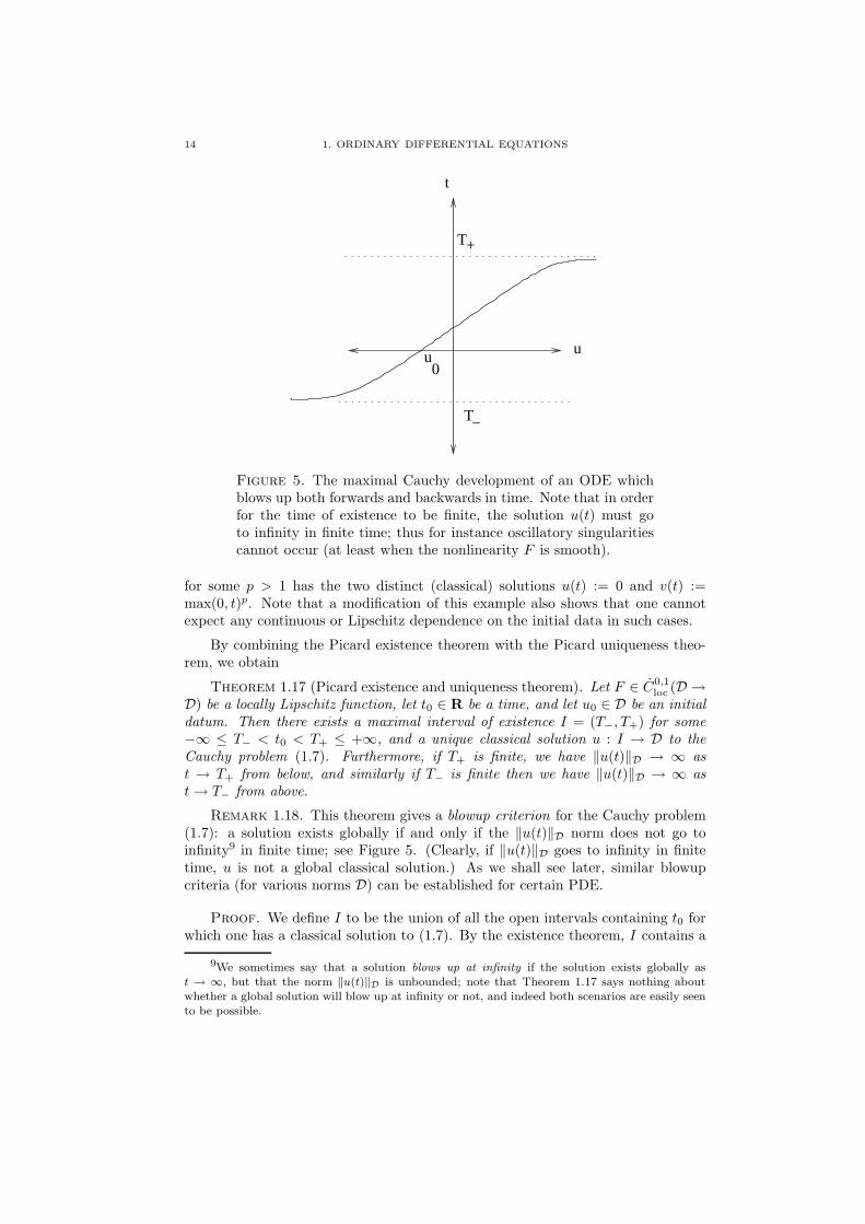
D) be a locally Lipschitz function, let t0 ∈ R be a time, and let u0 ∈ D be an initialdatum. Then there exists a maximal interval of existence I = (T−, T+) for some−∞ ≤ T− < t0 < T+ ≤ +∞, and a unique classical solution u : I → D to theCauchy problem (1.7). Furthermore, if T+ is finite, we have ‖u(t)‖D → ∞ ast → T+ from below, and similarly if T− is finite then we have ‖u(t)‖D → ∞ ast→ T− from above.
Remark 1.18. This theorem gives a blowup criterion for the Cauchy problem(1.7): a solution exists globally if and only if the ‖u(t)‖D norm does not go toinfinity9 in finite time; see Figure 5. (Clearly, if ‖u(t)‖D goes to infinity in finitetime, u is not a global classical solution.) As we shall see later, similar blowupcriteria (for various norms D) can be established for certain PDE.
Proof. We define I to be the union of all the open intervals containing t0 forwhich one has a classical solution to (1.7). By the existence theorem, I contains a
9We sometimes say that a solution blows up at infinity if the solution exists globally ast → ∞, but that the norm ‖u(t)‖D is unbounded; note that Theorem 1.17 says nothing aboutwhether a global solution will blow up at infinity or not, and indeed both scenarios are easily seento be possible.

1.2. GRONWALL’S INEQUALITY 15
neighbourhood of t0 and is clearly open and connected, and thus has the desiredform I = (T−, T+) for some −∞ ≤ T− < t0 < T+ ≤ +∞. By the uniquenesstheorem, we may glue all of these solutions together and obtain a classical solutionu : I → D on (1.7). Now suppose for contradiction that T+ was finite, and thatthere was some sequence of times tn approaching T+ from below for which ‖u(t)‖Dstayed bounded. On this bounded set (or on any slight enlargement of this set) Fis Lipschitz. Thus we may apply the existence theorem and conclude that one canextend the solution u to a short time beyond T+; gluing this solution to the existingsolution (again using the uniqueness theorem) we contradict the maximality of I.This proves the claim for T+, and the claim for T− is proven similarly.
The Picard theorem gives a very satisfactory local theory for the existence anduniqueness of solutions to the ODE (1.7), assuming of course that F is locallyLipschitz. The issue remains, however, as to whether the interval of existence(T−, T+) is finite or infinite. If one can somehow ensure that ‖u(t)‖D does notblow up to infinity at any finite time, then the above theorem assures us that theinterval of existence is all of R; as we shall see in the exercises, Gronwall’s inequalityis one method in which one can assure the absence of blowup. Another commonway to ensure global existence is to obtain a suitably “coercive” conservation law(e.g. energy conservation), which manages to contain the solution to a bounded set;see Proposition 1.24 below, as well as Section 1.4 for a fuller discussion. A thirdway is to obtain decay estimates, either via monotonicity formulae (see Section1.5) or some sort of dispersion or dissipation effect. We shall return to all of thesethemes throughout this monograph, in order to construct global solutions to variousequations.
Gronwall’s inequality is causal in nature; in its hypothesis, the value of theunknown function u(t) at times t is controlled by its value at previous times 0 <s < t, averaged against a function B(t) which can be viewed as a measure ofthe feedback present in the system; thus it is excessive feedback which leads toexponential growth (see Figure 4). This is of course very compatible with one’sintuition regarding cause and effect, and our interpretation of t as a time variable.However, in some cases, when t is not being interpreted as a time variable, onecan obtain integral inequalities which are acausal in that u(t) is controlled by anintegral of u(s) both for s < t and s > t. In many such cases, these inequalitieslead to no useful conclusion. However, if the feedback is sufficiently weak, and onehas some mild growth condition at infinity, one can still proceed as follows.
Theorem 1.19 (Acausal Gronwall inequality). Let 0 < α′ < α, 0 < β′ < βand ε, δ > 0 be real numbers. Let u : R → R+ be measurable and non-negative,and suppose that u obeys the integral inequality
(1.14) u(t) ≤ A(t) + δ
∫
R
min(e−α(s−t), e−β(t−s))u(s) ds
for all t ∈ R, where A : R → R+ is an arbitrary function. Suppose also that wehave the subexponential growth condition
supt∈R
e−ε|t|u(t) <∞.
16 1. ORDINARY DIFFERENTIAL EQUATIONS
Then if ε < min(α, β) and δ is sufficiently small depending on α, β, α′, β′, ε, wehave
(1.15) u(t) ≤ 2 sups∈R
min(e−α′(s−t), e−β
′(t−s))A(s).
for all t ∈ R.
Proof. We shall use an argument similar in spirit to that of the contractionmapping theorem, though in this case there is no actual contraction to iterate aswe have an integral inequality rather than an integral equation. By raising α′ andβ′ (depending on ε, α, β) if necessary we may assume ε < min(α′, β′). We willassume that there exists σ > 0 such that A(t) ≥ σeε|t| for all t ∈ R; the generalcase can then be deduced by replacing A(t) by A(t)+σeε|t| and then letting σ → 0,noting that the growth of the eε|t| factor will be compensated for by the decay ofthe min(e−α
′(s−t), e−β′(t−s)) factor since ε < min(α′, β′). Let B : R → R+ denote
the function
B(t) := sups∈R
min(e−α′(s−t), e−β
′(t−s))A(s).
Then we see that σeε|t| ≤ A(t) ≤ B(t), that B is strictly positive, and furthermoreB obeys the continuity properties
(1.16) B(s) ≤ max(eα′(s−t), eβ
′(t−s))B(t)
for all t, s ∈ R.Let M be the smallest real number such that u(t) ≤ MB(t) for all t ∈ R; our
objective is to show that M ≤ 2. Since B is bounded from below by σeε|t|, we seefrom the subexponential growth condition that M exists and is finite. From (1.14)we have
u(t) ≤ B(t) + δ
∫
R
min(e−α(s−t), e−β(t−s))u(s) ds.
Bounding u(s) by MB(s) and applying (1.16), we conclude
u(t) ≤ B(t) +MB(t)δ
∫
R
min(e−(α−α′)(s−t), e−(β−β′)(t−s)) ds.
Since 0 < α′ < α and 0 < β′ < β, the integral is convergent and is independent oft. Thus if δ is sufficiently small depending on α, β, α′, β′, we conclude that
u(t) ≤ B(t) +1
2MB(t)
which by definition of M implies M ≤ 1 + 12M . Since M is finite, we have M ≤ 2
as desired.
The above inequality was phrased for a continuous parameter t, but it quicklyimplies a discrete analogue:
Corollary 1.20 (Discrete acausal Gronwall inequality). Let 0 < α′ < α,0 < β′ < β, δ > 0, and 0 < ε < min(α, β) be real numbers. Let (un)n∈Z be asequence of non-negative numbers such that
(1.17) un ≤ An + δ∑
m∈Z
min(e−α(m−n), e−β(n−m))um

1.2. GRONWALL’S INEQUALITY 17
for all t ∈ R, where (An)n∈Z is an arbitrary non-negative sequence. Suppose alsothat we have the subexponential growth condition
supn∈Z
une−ε|n| <∞.
Then if δ is sufficiently small depending on α, β, α′, β′, ε, we have
(1.18) un ≤ 2 supm∈Z
min(e−α′(m−n), e−β
′(n−m))Am.
for all n ∈ Z.
This corollary can be proven by modifying the proof of the previous theorem,or alternatively by considering the function u(t) := u[t], where [t] is the nearestinteger to t; we leave the details to the reader. This corollary is particularly usefulfor understanding the frequency distribution of solutions to nonlinear dispersiveequations, in situations when the data is small (so the nonlinear effects of energytransfer between dyadic frequency ranges |ξ| ∼ 2n are weak). See for instance[Tao5], [Tao6], [Tao7] for ideas closely related to this. One can also use thesetypes of estimates to establish small energy regularity for various elliptic problemsby working in frequency space (the smallness is needed to make the nonlinear effectsweak).
Exercise 1.7 (Comparison principle). Let I = [t0, t1] be a compact interval,and let u : I → R, v : I → R be two scalar absolutely continuous functions. LetF ∈ C0,1
loc (I × R → R), and suppose that u and v obey the differential inequalities
∂tu(t) ≤ F (t, u(t)); ∂tv(t) ≥ F (t, v(t))
for all t ∈ I. Show that if u(t0) ≤ v(t0), then u(t) ≤ v(t) for all t ∈ [t0, t1], andsimilarly if u(t0) < v(t0), then u(t) < v(t) for all t ∈ [t0, t1]. (Hint: for the firstclaim, study the derivative of max(0, u(t) − v(t))2 and use Gronwall’s inequality.For the second, perturb the first argument by an epsilon.)
Exercise 1.8. Give an example to show that Theorem 1.10 fails when B ispermitted to be negative. Briefly discuss how this is consistent with the fact thatTheorem 1.12 still holds for negative B.
Exercise 1.9 (Sturm comparison principle). Let I be a time interval, and letu, v ∈ C2
loc(I → R) and a, f, g ∈ C0loc(I → R) be such that
∂2t u(t) + a(t)∂tu(t) + f(t)u(t) = ∂2
t v(t) + a(t)∂tv(t) + g(t)v(t) = 0
for all t ∈ I. Suppose also that v oscillates faster than u, in the sense that g(t) ≥ f(t)for all t ∈ I. Suppose also that u is not identically zero. Show that the zeroes ofv intersperse the zeros of u, in the sense that whenever t1 < t2 are times in Isuch that u(t1) = u(t2) = 0, then v has at least one zero in the interval [t1, t2].(Hint: reduce to the case when t1 and t2 are consecutive zeroes of u, and argue bycontradiction. By replacing u or v with −u or −v if necessary one may assume thatu, v are nonnegative on [t1, t2]. Obtain a first order equation for the Wronskianu∂tv−v∂tu.) This principle can be thought of as a substantial generalisation of theobservation that the zeroes of the sine and cosine functions intersperse each other.
Exercise 1.10. Let F ∈ C0,1loc (D → D) have at most linear growth, thus
‖F (u)‖D . 1 + ‖u‖D for all u ∈ D. Show that for each u0 ∈ D and t0 ∈ R
there exists a unique classical global solution u : R → D to the Cauchy problem

18 1. ORDINARY DIFFERENTIAL EQUATIONS
(1.7). Also, show that the solution maps St0(t) : D → D defined by St0(u0) = u(t0)are locally Lipschitz, obey the time translation invariance St0(t) = S0(t − t0), andthe group laws S0(t)S0(t
′) = S0(t + t′) and S0(0) = id. (Hint: use Gronwall’s in-equality to obtain bounds on ‖u(t)‖D in the maximal interval of existence (T−, T+)given by Theorem 1.17.) This exercise can be viewed as the limiting case p = 1 ofExercise 1.11 below.
Exercise 1.11. Let p > 1, let D be a finite-dimensional normed vector space,and let F ∈ C0,1
loc (D → D) have at most pth-power growth, thus ‖F (u)‖D . 1+‖u‖pDfor all u ∈ D. Let t0 ∈ R and u0 ∈ D, and let u : (T−, T+) → D be the maximalclassical solution to the Cauchy problem (1.7) given by the Picard theorem. Showthat if T+ is finite, then we have the lower bound
‖u(t)‖D &p (T+ − t)−1/(p−1)
as t approaches T+ from below, and similarly for T−. Give an example to showthat this blowup rate is best possible.
Exercise 1.12 (Slightly superlinear equations). Suppose F ∈ C0,1loc (D → D)
has at most x log x growth, thus
‖F (u)‖D . (1 + ‖u‖D) log(2 + ‖u‖D)
for all u ∈ D. Do solutions to the Cauchy problem (1.7) exist classically for all time(as in Exercise 1.10), or is it possible to blow up (as in Exercise 1.11)? In the lattercase, what is the best bound one can place on the growth of ‖u(t)‖D in time; inthe former case, what is the best lower bound one can place on the blow-up rate?
Exercise 1.13 (Persistence of constraints). Let u : I → D be a (classical)solution to the ODE ∂tu(t) = F (u(t)) for some time interval I and some F ∈C0
loc(D → D), and let H ∈ C1loc(D → R) be such that 〈F (v), dH(v)〉 = G(v)H(v)
for some G ∈ C0loc(D → R) and all v ∈ D; here we use
(1.19) 〈u, dH(v)〉 :=d
dεH(v + εu)|ε=0
to denote the directional derivative of H at v in the direction u. Show that ifH(u(t)) vanishes for one time t ∈ I, then it vanishes for all t ∈ I. Interpret thisgeometrically, viewing F as a vector field and studying the level surfaces of H . Notethat it is necessary that the ratio G between 〈F, dH〉 and H be continuous; it is notenough merely for 〈F, dH〉 to vanish whenever H does, as can be seen for instancefrom the counterexample H(u) = u2, F (u) = 2|u|1/2, u(t) = t2.
Exercise 1.14 (Compatibility of equations). Let F,G ∈ C1loc(D → D) have
the property that
(1.20) 〈F (v), dG(v)〉 − 〈G(v), dF (v)〉 = 0
for all v ∈ D. (The left-hand side has a natural interpretation as the Lie bracket[F,G] of the differential operators F ·∇, G ·∇ associated to the vector fields F andG.) Show that for any u0 ∈ D, there exists a neighbourhood B ⊂ R2 of the origin,and a map u ∈ C2(B → D) which satisfies the two equations
(1.21) ∂su(s, t) = F (u(s, t)); ∂tu(s, t) = G(u(s, t))
for all (s, t) ∈ B, with initial datum u(0, 0) = u0. Conversely, if u ∈ C2(B → D)solves (1.21) on B, show that (1.20) must hold for all v in the range of u. (Hint:

1.2. GRONWALL’S INEQUALITY 19
use the Picard existence theorem to construct u locally on the s-axis t = 0by using the first equation of (1.21), and then for each fixed s, extend u in thet direction using the second equation of (1.21). Use Gronwall’s inequality and(1.20) to establish that u(s, t) − u(0, t) −
∫ s0 F (u(s′, t)) ds′ = 0 for all (s, t) in a
neighbourhood of the origin.) This is a simple case of Frobenius’s theorem, regardingwhen a collection of vector fields can be simultaneously integrated.
Exercise 1.15 (Integration on Lie groups). Let H be a finite-dimensionalvector space, and let G be a Lie group in End(H) (i.e. a group of linear transfor-mations on H which is also a smooth manifold). Let g be the Lie algebra of G (i.e.
the tangent space of G at the identity). Let g0 ∈ G, and let X ∈ C0,1loc (R → g)
be arbitrary. Show that there exists a unique function g ∈ C1loc(R → G) such
that g(0) = g0 and ∂tg(t) = X(t)g(t) for all t ∈ R. (Hint: first use Gronwall’sinequality and Picard’s theorem to construct a global solution g : R → Mn(C)to the equation ∂tg(t) = X(t)g(t), and then use Gronwall’s inequality again,and local coordinate patches of G, to show that g stays on G.) Show that thesame claim holds if the matrix product X(t)g(t) is replaced by the Lie bracket[g(t), X(t)] := g(t)X(t) −X(t)g(t).
Exercise 1.16 (Levinson’s theorem). Let L ∈ C0(R → End(D)) be a time-dependent linear transformation acting on a finite-dimensional Hilbert space D, andlet F ∈ C0(R → D) be a time-dependent forcing term. Show that for every u0 ∈ Dthere exists a global solution u ∈ C0
loc(R → D) to the ODE ∂tu = L(t)u + F (t),with the bound
|u(t)| ≤ (|u0|D +
∫ t
0
|F (s)|D ds) exp(
∫ t
0
‖(L(t) + L∗(t))/2‖op dt)
for all t ≥ 0. (Hint: control the evolution of |u(t)|2 = 〈u(t), u(t)〉D .) Thus one canobtain global control on a linear ODE with arbitrarily large coefficients, as long asthe largeness is almost completely contained in the skew-adjoint component of thelinear operator. In particular, if F and the self-adjoint component of L are bothabsolutely integrable, conclude that u(t) is bounded uniformly in t.
Exercise 1.17. Give examples to show that Theorem 1.19 and Corollary 1.20fail (even when A is identically zero) if ε or δ become too large, or if the hypothesisthat u has subexponential growth is dropped.
Exercise 1.18. Let α, δ > 0, let d ≥ 1 be an integer, let 0 ≤ γ < d, and letu : Rd → R+ and A : Rd → R+ be locally integrable functions such that one hasthe pointwise inequality
u(x) ≤ A(x) + δ
∫
Rd
e−α|x−y|
|x− y|γ u(y) dy
for almost every x ∈ Rd. Suppose also that u is a tempered distribution in additionto a locally integrable function. Show that if 0 < α′ < α and δ is sufficiently smalldepending on α, α′, γ, then we have the bound
u(x) ≤ 2‖e−α′|x−y|A(y)‖L∞y (Rd)
for almost every x ∈ Rd. (Hint: you will need to regularise u first, averaging on asmall ball, in order to convert the tempered distribution hypothesis into a pointwisesubexponential bound. Then argue as in Proposition 1.19. One can then take limitsat the end using the Lebesgue differentiation theorem.)

20 1. ORDINARY DIFFERENTIAL EQUATIONS
Exercise 1.19 (Singular ODE). Let F,G ∈ C0,1(D → D) be Lipschitz mapswith F (0) = 0 and ‖F‖C0,1(D→D) < 1. Show that there exists a T > 0 for
which there exists a unique classical solution u : (0, T ] → D to the singularnon-autonomous ODE ∂tu(t) = 1
tF (u(t)) + G(u(t)) with the boundary condi-tion lim supt→0 ‖u(t)‖D/t < ∞ as t → 0. (Hint: For uniqueness, use a Gronwallinequality argument. For existence, construct iterates in the space of functionstv : v ∈ C0([0, T ] → D).) Show that u in fact extends to a C1 function on [0, T ]with u(0) = 0 and ∂tu(0) = G(0). Also give an example to show that uniquenesscan break down when the Lipschitz constant of F exceeds 1. (You can take a verysimple example, for instance with F linear and G zero.)
1.3. Bootstrap and continuity arguments
If you have built your castles in the air, your work need not be lost;that is where they should be. Now put the foundations under them.(Henry David Thoreau, “Walden”)
The Picard existence theorem allows us to construct solutions to ODE such as∂tu(t) = F (u(t)) on various time intervals. Once these solutions have been con-structed, it is natural to then ask what kind of quantitative estimates and asymp-totics these solutions satisfy, especially over long periods of time. If the equation isfortunate enough to be solvable exactly (which can happen for instance if the equa-tion is completely integrable), then one can read off the desired estimates from theexact solution, in principle at least. However, in the majority of cases no explicitsolution is available10. Many times, the best one can do is to write the solutionu(t) in terms of itself, using the strong solution concept. For instance, if the initialcondition is u(t0) = u0, then we have
(1.22) u(t) = u0 +
∫ t
t0
F (u(s)) ds.
This equation tells us that if we have some information on u (for instance, if wecontrol some norm ‖‖Y of u(s)), we can insert this information into the right-hand side of the above integral equation (together with some knowledge of theinitial datum u0 and the nonlinearity F ), and conclude some further control of thesolution u (either in the same norm ‖‖Y , or in some new norm).
Thus we can use equations such as (1.22) to obtain control on u - but only if onestarts with some control on u in the first place. Thus it seems difficult to get startedwhen executing this strategy, since one often starts with only very little control onu, other than continuity. Nevertheless there is a simple principle, of almost magicalpower, that allows one to assume “for free” that u already obeys some quantitativebound, in order to prove that u obeys another quantitative bound - as long asthe bound one ends up proving is slightly stronger than the bound one used as ahypothesis (to avoid circularity). This principle - which is a continuous analogue
10Of course, the contraction mapping argument used in Theorem 1.7 does in principle givea description of the solution, at least locally, as the limit of iterates of a certain integral map Φ,and the Cauchy-Kowalevski theorem in principle gives a Taylor series expansion of the solution.However in practice these expansions are rather complicated, and only useful for analyzing theshort-time behaviour and not long-time behaviour. Even if an explicit solution (e.g. involvingspecial functions) is available, it may be easier to read off the asymptotics and other features ofthe equation from an analytic argument such as a bootstrap argument than from inspection ofthe explicit solution.
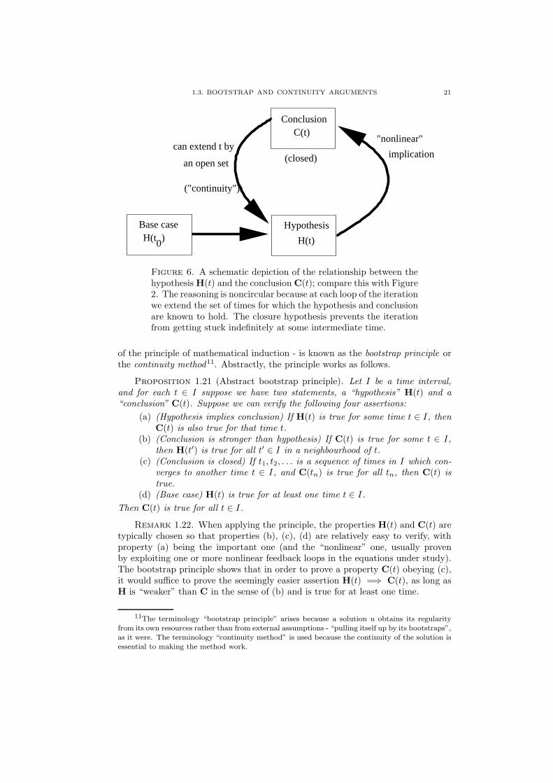
1.3. BOOTSTRAP AND CONTINUITY ARGUMENTS 21
0
Base caseH(t )
(closed)
H(t)
Hypothesis
ConclusionC(t)
can extend t by
an open set
("continuity")
"nonlinear"
implication
Figure 6. A schematic depiction of the relationship between thehypothesis H(t) and the conclusion C(t); compare this with Figure2. The reasoning is noncircular because at each loop of the iterationwe extend the set of times for which the hypothesis and conclusionare known to hold. The closure hypothesis prevents the iterationfrom getting stuck indefinitely at some intermediate time.
of the principle of mathematical induction - is known as the bootstrap principle orthe continuity method11. Abstractly, the principle works as follows.
Proposition 1.21 (Abstract bootstrap principle). Let I be a time interval,and for each t ∈ I suppose we have two statements, a “hypothesis” H(t) and a“conclusion” C(t). Suppose we can verify the following four assertions:
(a) (Hypothesis implies conclusion) If H(t) is true for some time t ∈ I, thenC(t) is also true for that time t.
(b) (Conclusion is stronger than hypothesis) If C(t) is true for some t ∈ I,then H(t′) is true for all t′ ∈ I in a neighbourhood of t.
(c) (Conclusion is closed) If t1, t2, . . . is a sequence of times in I which con-verges to another time t ∈ I, and C(tn) is true for all tn, then C(t) istrue.
(d) (Base case) H(t) is true for at least one time t ∈ I.
Then C(t) is true for all t ∈ I.
Remark 1.22. When applying the principle, the properties H(t) and C(t) aretypically chosen so that properties (b), (c), (d) are relatively easy to verify, withproperty (a) being the important one (and the “nonlinear” one, usually provenby exploiting one or more nonlinear feedback loops in the equations under study).The bootstrap principle shows that in order to prove a property C(t) obeying (c),it would suffice to prove the seemingly easier assertion H(t) =⇒ C(t), as long asH is “weaker” than C in the sense of (b) and is true for at least one time.
11The terminology “bootstrap principle” arises because a solution u obtains its regularityfrom its own resources rather than from external assumptions - “pulling itself up by its bootstraps”,as it were. The terminology “continuity method” is used because the continuity of the solution isessential to making the method work.

22 1. ORDINARY DIFFERENTIAL EQUATIONS
Proof. Let Ω be the set of times t ∈ I for which C(t) holds. Properties (d)and (a) ensure that Ω is non-empty. Properties (b) and (a) ensure that Ω is open.Property (c) ensures that Ω is closed. Since the interval I is connected, we thus seethat Ω = I, and the claim follows.
More informally, one can phrase the bootstrap principle as follows:
Principle 1.23 (Informal bootstrap principle). If a quantity u can be boundedin a nontrivial way in terms of itself, then under reasonable conditions, one canconclude that u is bounded unconditionally.
We give a simple example of the bootstrap principle in action, establishingglobal existence for a system in a locally stable potential well from small initialdata.
Proposition 1.24. Let D be a finite-dimensional Hilbert space, and let V ∈C2
loc(D → R) be such that such that V (0) = 0, ∇V (0) = 0, and ∇2V (0) is strictlypositive definite. Then for all u0, u1 ∈ D sufficiently close to 0, there is a uniqueclassical global solution u ∈ C2
loc(R → D) to the Cauchy problem
(1.23) ∂2t u(t) = −∇V (u(t)); u(0) = u0; ∂tu(0) = u1.
Furthermore, this solution stays bounded uniformly in t.
Remark 1.25. The point here is that the potential well V is known to be stablenear zero by hypothesis, but could be highly unstable away from zero; see Figure7. Nevertheless, the bootstrap argument can be used to prevent the solution from“tunnelling” from the stable region to the unstable region.
Proof. Applying the Picard theorem (converting the second-order ODE intoa first-order ODE in the usual manner) we see that there is a maximal intervalof existence I = (T−, T+) containing 0, which supports a unique classical solutionu ∈ C2
loc(I → D) to the Cauchy problem (1.23). Also, if T+ is finite, then we havelimt→T+ ‖u(t)‖D + ‖∂tu(t)‖D = ∞, and similarly if T− is finite.
For any time t ∈ I, let E(t) denote the energy
(1.24) E(t) :=1
2‖∂tu(t)‖2
D + V (u(t)).
From (1.23) we see that
∂tE(t) = 〈∂tu(t), ∂2t u(t)〉 + 〈∂tu(t),∇V (u(t))〉 = 0
and thus we have the conservation law
E(t) = E(0) =1
2‖u1‖2
D + V (u0).
If u0, u1 are sufficiently close to 0, we can thus make E(t) = E(0) as small asdesired.
The problem is that we cannot quite conclude from the smallness of E that uis itself small, because V could turn quite negative away from the origin. However,such a scenario can only occur when u is large. Thus we need to assume that u issmall in order to prove that u is small. This may seem circular, but fortunately thebootstrap principle allows one to justify this argument.
Let ε > 0 be a parameter to be chosen later, and let H(t) denote the statement
‖∂tu(t)‖2D + ‖u(t)‖2
D ≤ (2ε)2
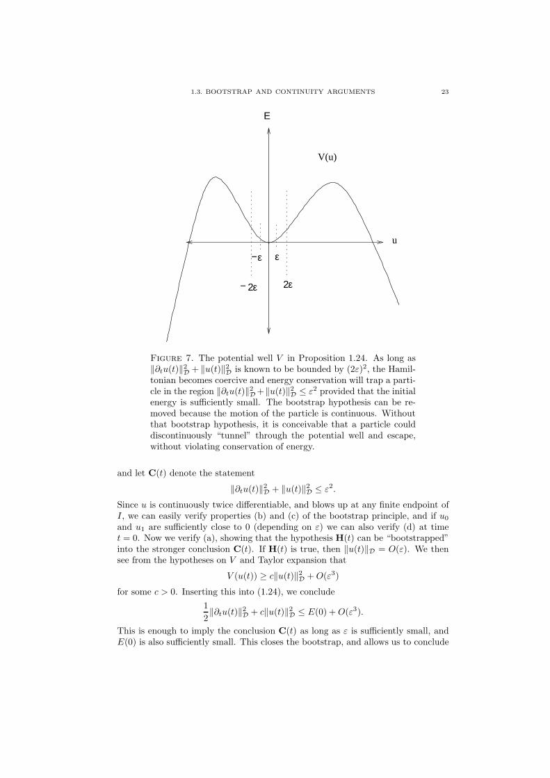
1.3. BOOTSTRAP AND CONTINUITY ARGUMENTS 23
u
V(u)
ε ε
2ε2ε−
−
Ε
Figure 7. The potential well V in Proposition 1.24. As long as‖∂tu(t)‖2
D + ‖u(t)‖2D is known to be bounded by (2ε)2, the Hamil-
tonian becomes coercive and energy conservation will trap a parti-cle in the region ‖∂tu(t)‖2
D +‖u(t)‖2D ≤ ε2 provided that the initial
energy is sufficiently small. The bootstrap hypothesis can be re-moved because the motion of the particle is continuous. Withoutthat bootstrap hypothesis, it is conceivable that a particle coulddiscontinuously “tunnel” through the potential well and escape,without violating conservation of energy.
and let C(t) denote the statement
‖∂tu(t)‖2D + ‖u(t)‖2
D ≤ ε2.
Since u is continuously twice differentiable, and blows up at any finite endpoint ofI, we can easily verify properties (b) and (c) of the bootstrap principle, and if u0
and u1 are sufficiently close to 0 (depending on ε) we can also verify (d) at timet = 0. Now we verify (a), showing that the hypothesis H(t) can be “bootstrapped”into the stronger conclusion C(t). If H(t) is true, then ‖u(t)‖D = O(ε). We thensee from the hypotheses on V and Taylor expansion that
V (u(t)) ≥ c‖u(t)‖2D +O(ε3)
for some c > 0. Inserting this into (1.24), we conclude
1
2‖∂tu(t)‖2
D + c‖u(t)‖2D ≤ E(0) +O(ε3).
This is enough to imply the conclusion C(t) as long as ε is sufficiently small, andE(0) is also sufficiently small. This closes the bootstrap, and allows us to conclude

24 1. ORDINARY DIFFERENTIAL EQUATIONS
2A
A
u
Α
A + F(u)
u
ε
hereu forbidden
2A
Figure 8. A depiction of the situation in Exercise 1.21. Note theimpenetrable barrier in the middle of the u domain.
that C(t) is true for all t ∈ I. In particular, I must be infinite, since we knowthat ‖∂tu(t)‖2
D + ‖u(t)‖2D would blow up at any finite endpoint of I, and we are
done.
One can think of the bootstrap argument here as placing an “impenetrablebarrier”
ε2 < ‖∂tu(t)‖2D + ‖u(t)‖2
D ≤ (2ε)2
in phase space. Property (a) asserts that the system cannot venture into thisbarrier. Properties (b), (c) ensure that this system cannot “jump” from one sideof the barrier to the other instantaneously. Property (d) ensures that the systemstarts out on the “good” side of the barrier. We can then conclude that the systemstays in the good side for all time; see Figure 7. Note also the division of labourin proving these properties. The properties (b), (c) are proven using the localexistence theory (i.e. Theorem 1.17). The property (d) comes from the hypotheseson the initial datum. The property (a) requires some structural information on theequation, in this case the existence of a conserved energy E(t) with enough locally“coercive” properties to contain the system within the desired barrier. This patternof argument is very common in the analysis of nonlinear ODE and PDE, and weshall see several more examples of this later in this monograph.
Exercise 1.20. Show by example that Proposition 1.21 fails if any one of itsfour hypotheses are removed.
Exercise 1.21. Let I be a time interval, and u ∈ C0loc(I → R+) be a non-
negative function obeying the inequality
(1.25) u(t) ≤ A+ εF (u(t))
1.3. BOOTSTRAP AND CONTINUITY ARGUMENTS 25
for some A, ε > 0 and some function F : R+ → R+ which is locally bounded.Suppose also that u(t0) ≤ 2A for some t0 ∈ I. If ε is sufficiently small dependingon A and F , show that in fact u(t) ≤ 2A for all t ∈ I. Show that the conclusioncan fail if u is not continuous or ε is not small. Note however that no assumptionis made on the growth of F at infinity. Informally speaking, this means that ifone ever obtains an estimate of the form u ≤ A + εF (u), then one can drop theεF (u) term (at the cost of increasing the main term A by a factor of 2) providedthat ε is suitably small, some initial condition is verified, and some continuity isavailable. This is particularly useful for showing that a nonlinear solution obeysalmost the same estimates as a linear solution if the nonlinear effect is sufficientlyweak. Compare this with Principle 1.23.
Exercise 1.22. Let I be a time interval, and let u ∈ C0loc(I → R+) obey the
inequalityu(t) ≤ A+ εF (u(t)) +Bu(t)θ
for some A,B, ε > 0 and 0 < θ < 1, and some locally bounded function F : R+ →R+. Suppose also that u(t0) ≤ A′ for some t0 ∈ I and A′ > 0. Show that if ε issufficiently small depending on A,A′, B, θ, F , then we have u(t) .θ A+B1/(1−θ) forall t ∈ I. Thus we can tolerate an additional u-dependent term on the right-handside of (1.25) as long as it grows slower than linearly in u.
Exercise 1.23 (Compactness solutions). Let t0 ∈ R be a time, let u0 ∈ D,and let F : D → D be a function which is continuous (and hence bounded) in aneighbourhood of u0. Show that there exists an open time interval I containingt0, and a classical solution u ∈ C1(I → D) to the Cauchy problem (1.7). (Hint:approximate F by a sequence of Lipschitz functions Fm and apply Theorem 1.17to obtain solutions um to the problem ∂tum = Fm(um) on some maximal interval(T−,m, T+,m). Use a bootstrap argument and Gronwall’s inequality to show thatfor some fixed open interval I (independent of m) containing t0, the solutions umwill stay uniformly bounded and uniformly Lipschitz (hence equicontinuous) in thisinterval, and that this interval is contained inside all of the (T−,m, T+,m). Thenapply the Arzela-Ascoli theorem to extract a uniformly convergent subsequence ofthe um on I, and see what happens to the integral equations um(t) = um(t0) +∫ tt0Fm(um(s)) ds in the limit, using Lemma 1.3 if necessary.) This is a simple
example of a compactness method to construct solutions to equations such as (1.13),for which uniqueness is not available.
Exercise 1.24 (Persistence of constraints, II). Let u : [t0, t1] → D be a classicalsolution to the ODE ∂tu(t) = F (u(t)) for some continuous F : D → D, and letH1, . . . , Hn ∈ C1
loc(D → R) have the property that
〈F (v), dHj(v)〉 ≥ 0
whenever 1 ≤ j ≤ n and v ∈ D is such that Hj(v) = 0 and Hi(v) ≥ 0 for all1 ≤ i ≤ n. Show that if the statement
Hi(u(t)) ≥ 0 for all 1 ≤ i ≤ n
is true at time t = t0, then it is true for all times t ∈ [t0, t1]. Compare this resultwith Exercise 1.13.
Exercise 1.25 (Forced blowup). Let k ≥ 1, and let u : [0, T∗) → R be aclassical solution to the equation ∂kt u(t) = F (u(t)), where F : R → R is continuous.

26 1. ORDINARY DIFFERENTIAL EQUATIONS
Suppose that u(0) > 0 and ∂jt u(0) ≥ 0 for all 1 ≤ j < k, and suppose that one hasthe lower bound such that F (v) & vp for all v ≥ u(0) and some p > 1. Concludethe upper bound T∗ .p,k u(0)(1−p)/k on the time of existence. (Hint: first establish
that u(t) ≥ u(0) and ∂jt u(t) ≥ 0 for all 1 ≤ j < k and 0 ≤ t < T∗, for instance byusing Exercise 1.24. Then bootstrap these bounds to obtain some estimate on thedoubling time of u, in other words to obtain an upper bound on the first time t forwhich u(t) reaches 2u(0).) This shows that equations of the form ∂kt u(t) = F (u(t))can blow up if the initial datum is sufficiently large and positive.
Exercise 1.26. Use the continuity method to give another proof of Gronwall’sinequality (Theorem 1.10). (Hint: for technical reasons it may be easier to first
prove that u(t) ≤ (1 + ε)A exp(∫ tt0B(s) ds) for each ε > 0, as continuity arguments
generally require “an epsilon of room”.) This alternate proof of Gronwall’s inequal-ity is more robust, as it can handle additional nonlinear terms on the right-handside provided that they are suitably small.
1.4. Noether’s theorem
Now symmetry and consistency are convertible terms - thus Poetryand Truth are one. (Edgar Allen Poe, “Eureka: A Prose Poem”)
A remarkable feature of many important differential equations, especially thosearising from mathematical physics, is that their dynamics, while complex, still con-tinue to maintain a certain amount of unexpected structure. One of the mostimportant examples of such structures are conservation laws - certain scalar quan-tities of the system that remain constant throughout the evolution of the system;another important example are symmetries of the equation - that there often existsa rich and explicit group of transformations which necessarily take one solutionof the equation to another. A remarkable result of Emmy Noether shows thatthese two structures are in fact very closely related, provided that the differentialequation is Hamiltonian; as we shall see, many interesting nonlinear dispersive andwave equations will be of this type. Noether’s theorem is one of the fundamentaltheorems of Hamiltonian mechanics, and has proven to be extremely fruitful in theanalysis of such PDE. Of course, the field of Hamiltonian mechanics offers manymore beautiful mathematical results than just Noether’s theorem; it is of great in-terest to see how much else of this theory (which is still largely confined to ODE)can be extended to the PDE setting. See [Kuk3] for some further discussion.
Noether’s theorem can be phrased symplectically, in the context of Hamiltonianmechanics, or variationally, in the context of Lagrangian mechanics. We shall optto focus almost exclusively on the former; the variational perspective has certainstrengths for the nonlinear PDE we shall analyse (most notably in elucidating therole of the stress-energy tensor, and of the distinguished role played by groundstates) but we will not pursue it in detail here (though see Exercises 1.44, 1.45,2.60). We shall content ourselves with describing only a very simple special case ofthis theorem; for a discussion of Noether’s theorem in full generality, see [Arn].
Hamiltonian mechanics can be defined on any symplectic manifold, but forsimplicity we shall restrict our attention to symplectic vector spaces.
Definition 1.26. A symplectic vector space (D, ω) is a finite-dimensional realvector space D, equipped with a symplectic form ω : D×D → R, which is bilinearand anti-symmetric, and also non-degenerate (so for each non-zero u ∈ D there

1.4. NOETHER’S THEOREM 27
exists a v ∈ D such that ω(u, v) 6= 0). Given any H ∈ C1loc(D → R), we define the
symplectic gradient ∇ωH ∈ C0loc(D → D) to be the unique function such that
(1.26) 〈v, dH(u)〉 =d
dεH(u+ εv)|ε=0 = ω(∇ωH(u), v);
this definition is well-defined thanks to the non-degeneracy of ω and the finitedimensionality of D. Given two functions H,E ∈ C1
loc(D → R), we define thePoisson bracket H,E : D → R by the formula
(1.27) H,E(u) := ω(∇ωH(u),∇ωE(u)).
A Hamiltonian function on a phase space (D, ω) is any function12 H ∈ C2loc(D →
R); to each such Hamiltonian, we associate the corresponding Hamiltonian flow
(1.28) ∂tu(t) = ∇ωH(u(t)).
Note that with this definition, Hamiltonian ODE (1.28) are automatically au-tonomous (time-translation-invariant). However it is possible to consider time-varying Hamiltonians also: see Exercise 1.42. Note that the Hamiltonian of anequation is only determined up to a constant, since replacing H by H+C does notaffect the symplectic gradient of H .
Example 1.27. If
D := Rn × Rn = (q1, . . . , qn, p1, . . . , pn) : q1, . . . , qn, p1, . . . , pn ∈ Rfor some n ≥ 1, and ω : D ×D → R is the bilinear form
ω :=
n∑
j=1
dqj ∧ dpj
or in other words
ω((q1, . . . , qn, p1, . . . , pn), (q′1, . . . , q
′n, p
′1, . . . , p
′n)) :=
n∑
j=1
p′jqj − pjq′j
then (D, ω) is symplectic, and for any H,E ∈ C1loc(D → R) we have
∇ωH = (∂H
∂p1, . . . ,
∂H
∂pn,−∂H
∂q1, . . . ,− ∂H
∂qn)
and
H,E =
n∑
j=1
∂H
∂pj
∂E
∂qj− ∂H
∂qj
∂E
∂pj.
In particular, the Hamiltonian ODE associated to a Hamiltonian function H ∈C2
loc(D → R) is given by Hamilton’s equations of motion
(1.29) ∂tqj(t) =∂H
∂pj(q(t), p(t)); ∂tpj(t) = −∂H
∂qj(q(t), p(t)),
where we write
u(t) = (q(t), p(t)); q(t) = (q1(t), . . . , qn(t)); p(t) = (p1(t), . . . , pn(t)).
12One can weaken this hypothesis of continuous twice differentiability and still define aHamiltonian flow, but the theory becomes more delicate and we will not address it here.

28 1. ORDINARY DIFFERENTIAL EQUATIONS
Thus, for instance, if H takes the form
(1.30) H(q, p) =1
2m|p|2 + V (q)
where |p|2 := p21 + . . . + p2
n, m > 0 is a constant, and V ∈ C2loc(R
n → R), thenHamilton’s equations become Newton’s laws of motion
∂tq(t) =1
mp(t); ∂tp(t) = −∇V (q(t)).
Example 1.28. Let D = Cn be endowed with the symplectic form
(1.31) ω :=n∑
j=1
1
2Im(dzj ∧ dzj)
or in other words
ω((z1, . . . , zn), (z′1, . . . , z
′n)) :=
n∑
j=1
Im(zjz′j).
Then for any H,E ∈ C1loc(D → R) we have
∇ωH = (2i∂H
∂z1, . . . , 2i
∂H
∂zn)
and
H,E = 4
n∑
j=1
Im(∂H
∂zj
∂E
∂zj)
where ∂H∂z := ∂H
∂x − i∂H∂y and ∂H∂z := ∂H
∂x + i∂H∂y . Thus for instance if H is the simple
harmonic oscillator
(1.32) H(z) :=
n∑
j=1
1
2λj |zj |2
for some λ1, . . . , λn ∈ R, then the equations of motion are
∂tzj(t) = iλjzj(t).
This is in fact the canonical form for any quadratic Hamiltonian; see Exercise1.41.
Hamiltonian equations enjoy a number of good properties. SinceH ∈ C2loc(D →
R), the function ∇ωH ∈ C0,1loc (D → D) is locally Lipschitz, and so the Picard
existence theorem applies; in particular, for any bounded set Ω ⊂ D, there is apositive time T > 0 for which we have Lipschitz flow maps S(t) = S0(t) ∈ C0,1(Ω →D) defined for |t| ≤ T . In the quadratic growth case when ∇2H is bounded, then
∇ωH is globally Lipschitz, and one thus has global flow maps S(t) ∈ C0,1loc (D → D)
defined for all times t ∈ R (by Exercise 1.10). These maps obey the group lawsS(t + t′) = S(t)S(t′), S(0) = id. Furthemore the S(t) are diffeomorphisms andsymplectomorphisms; see Exercise 1.4 and Exercise 1.32.
Let H,E ∈ C2loc(D → R) be two Hamiltonians on a symplectic phase space
(D, ω), and let u ∈ C1loc(I → D) be a classical solution to the Hamiltonian ODE

1.4. NOETHER’S THEOREM 29
(1.28). From the chain rule and (1.26), (1.27), we thus have the Poisson equation13
(1.33)d
dtE(u(t)) = H,E(u(t)).
Let us say that a quantity E is conserved by (1.28) if E(u(t)) is constant forany (classical) solution u : I → D of (1.28). From (1.33) and the anti-symmetryH,E = −E,H of the Poisson bracket, we conclude
Theorem 1.29 (Noether’s theorem). Let H and E be two Hamiltonians on asymplectic phase space (D, ω). Then the following are equivalent.
(a) H,E = 0.(b) The quantity E is conserved by the Hamiltonian flow of H.(c) The quantity H is conserved by the Hamiltonian flow of E.
If any of the above three properties hold, we say that H and E Poisson com-mute. As stated, Noether’s theorem is symmetric in H and E. However, thistheorem is often interpreted in a somewhat asymmetric way. Assume for sake ofargument that the flow maps SE(t) of E are globally defined (this is the case, for in-stance, if E is quadratic growth). We view the flow maps SE(t) as a one-dimensionalgroup action on the phase space D. Noether’s theorem then asserts that E is a con-served quantity for the equation (1.28) if and only if H is symmetric (i.e. invariant)with respect to the group actions SE(t); for a generalisation to higher-dimensionalgroup actions, see Exercise 1.34. Thus this theorem gives a very satisfactory linkbetween the symmetries of the Hamiltonian H to the conserved quantities of theflow (1.28). The larger the group of symmetries, the more conserved quantities oneobtains14.
For instance, since H clearly Poisson commutes with itself, we see that Hitself is a conserved quantity, thus H(u(t0)) = H(u0) for any classical solutionu ∈ C1
loc(I → D) to the Cauchy problem
(1.34) ∂tu(t) = ∇ωH(u(t)); u(t0) = u0.
As another example, if (D, ω) is the complex phase space given in Example 1.28,and the Hamiltonian is invariant under phase rotations, thus
H(eiθz1, . . . , eiθzn) = H(z1, . . . , zn) for all z1, . . . , zn ∈ C, θ ∈ R
then the total charge∑nj=1 |zj |2 is conserved by the flow. Indeed, the phase rotation
is (up to a factor of two) nothing more than the Hamiltonian flow associated to thetotal charge.
Another class of important examples concerns the phase space (Rd ×Rd)N ofN particles in Rd, parameterised by N position variables q1, . . . , qN ∈ Rd and N
13This equation is unrelated to the PDE ∆u = ρ, which is sometimes also referred to asPoisson’s equation.
14Provided, of course, that the symmetries themselves come from Hamiltonian flows. Certainsymmetries, notably scaling symmetries, are thus difficult to place in this framework, as they
typically violate Louville’s theorem and thus cannot be Hamiltonian flows, though they do tendto generate almost conserved quantities, such as that arising in the virial identity. Also, discretesymmetries such as time reversal symmetry or permutation symmetry also are not in the rangeof applicability for Noether’s theorem.

30 1. ORDINARY DIFFERENTIAL EQUATIONS
Table 1. Some common symmetry groups and their associatedconservation laws (or approximate conservation laws, in the case ofthe virial identity). Not all of these follow directly from Noether’stheorem as stated, and are best viewed instead using the “La-grangian” approach to this theorem. In some cases, the interpre-tation of the conserved quantity depends on the equation; for in-stance spatial translation corresponds to momentum for wave andSchrodinger equations, but corresponds instead to mass for KdVtype equations.
Symmetry Conserved quantitytime translation energy / Hamiltonianspatial translation momentum / massspatial rotation angular momentumGalilean transformation (renormalised) centre-of-massLorentz transformation (renormalised) centre-of-energyscaling (virial identity)base space diffeomorphism stress-energyphase rotation mass / probability / chargegauge transform charge
momentum variables p1, . . . , pN ∈ Rd, with the symplectic form
ω :=
N∑
j=1
dqj ∧ dpj =
N∑
j=1
d∑
i=1
dqj,i ∧ dpj,i.
If a Hamiltonian H(q1, . . . , qN , p1, . . . , pN) is invariant under spatial translations,thus
H(q1 − x, . . . , qN − x, p1, . . . , pN) = H(q1, . . . , qN , p1, . . . , pN)
for all x, p1, . . . , pN , q1, . . . , qN ∈ Rd, then Noether’s theorem implies that the total
momentum p =∑N
j=1 pj is conserved by the flow. If the Hamiltonian takes theform
(1.35) H(q1, . . . , qN , p1, . . . , pN) =
N∑
j=1
1
2mi|pi|2 + V (q1, . . . , qN )
for some (translation invariant) potential V ∈ C2loc((R
d)N → R), then the totalmomentum takes the familiar form
p =
N∑
j=1
mjdqjdt.
Similarly, if the Hamiltonian is invariant under angular rotations U : Rd → Rd,thus
H(Uq1, . . . , UqN , Up1, . . . , UpN ) = H(q1, . . . , qN , p1, . . . , pN )
for all p1, . . . , pN , q1, . . . , qN ∈ Rd and U ∈ SO(d), then Noether’s theorem (or moreprecisely the generalisation in Exercise 1.34) implies that the angular momentum
L :=∑Nj=1 qj ∧ pj ∈
∧2Rd is also preserved by the flow.
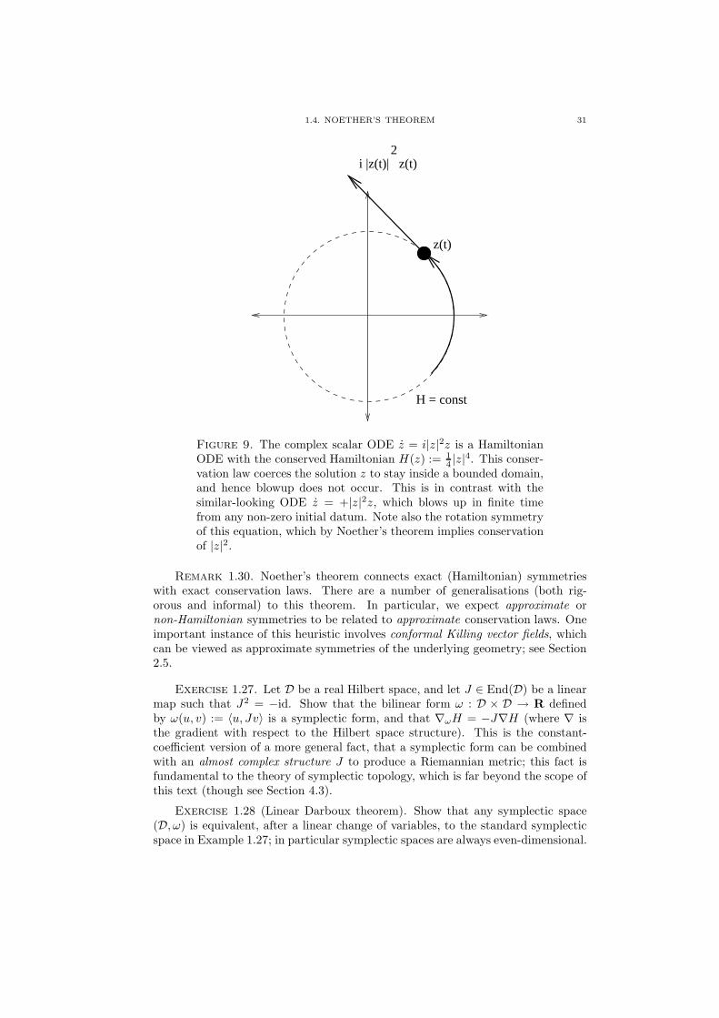
1.4. NOETHER’S THEOREM 31
H = const
z(t)
i |z(t)| z(t)2
Figure 9. The complex scalar ODE z = i|z|2z is a HamiltonianODE with the conserved Hamiltonian H(z) := 1
4 |z|4. This conser-vation law coerces the solution z to stay inside a bounded domain,and hence blowup does not occur. This is in contrast with thesimilar-looking ODE z = +|z|2z, which blows up in finite timefrom any non-zero initial datum. Note also the rotation symmetryof this equation, which by Noether’s theorem implies conservationof |z|2.
Remark 1.30. Noether’s theorem connects exact (Hamiltonian) symmetrieswith exact conservation laws. There are a number of generalisations (both rig-orous and informal) to this theorem. In particular, we expect approximate ornon-Hamiltonian symmetries to be related to approximate conservation laws. Oneimportant instance of this heuristic involves conformal Killing vector fields, whichcan be viewed as approximate symmetries of the underlying geometry; see Section2.5.
Exercise 1.27. Let D be a real Hilbert space, and let J ∈ End(D) be a linearmap such that J2 = −id. Show that the bilinear form ω : D × D → R definedby ω(u, v) := 〈u, Jv〉 is a symplectic form, and that ∇ωH = −J∇H (where ∇ isthe gradient with respect to the Hilbert space structure). This is the constant-coefficient version of a more general fact, that a symplectic form can be combinedwith an almost complex structure J to produce a Riemannian metric; this fact isfundamental to the theory of symplectic topology, which is far beyond the scope ofthis text (though see Section 4.3).
Exercise 1.28 (Linear Darboux theorem). Show that any symplectic space(D, ω) is equivalent, after a linear change of variables, to the standard symplecticspace in Example 1.27; in particular symplectic spaces are always even-dimensional.

32 1. ORDINARY DIFFERENTIAL EQUATIONS
(Hint: induct on the dimension of D. If the dimension is non-zero, use the non-degeneracy of ω to locate two linearly independent vectors u, v ∈ D such thatω(u, v) 6= 0. Then restrict to the symplectic complement w ∈ D : ω(u,w) =ω(v, w) = 0 and use the induction hypothesis.) Note that this change of variableswill usually not be unique. Conclude in particular that every symplectic phasespace has an even number of dimensions.
Exercise 1.29. Show that if H ∈ C2loc(D → R) is a Hamiltonian which has a
non-degenerate local minimum at some u0 ∈ D (thus ∇H(u0) = 0 and ∇2H(u0) isstrictly positive definite), then one has global solutions to the associated Hamilton-ian equation as soon as the initial datum u0 is sufficiently close to u0. Note thatthis generalises Proposition 1.24; indeed, one can proceed by a modification of theproof of that proposition. Similarly, show that if H is a Hamiltonian which is glob-ally coercive in the sense that limv→∞ |H(v)| = ∞, then one has global solutionsto the associated Hamiltonian equation for arbitrary initial data.
Exercise 1.30. Show that if one applies the time reversal change of variablet 7→ −t to a Hamiltonian equation, one obtains another Hamiltonian equation;what is the new Hamiltonian?
Exercise 1.31. Let I be a time interval, and let (D, ω), (D′, ω′) be symplec-tic vector spaces. Let u ∈ C1
loc(I → D) solve a Hamiltonian equation ∂tu(t) =∇ωH(u(t)) for some Hamiltonian H ∈ C2
loc(D → R), and let u′ ∈ C1loc(I → D′)
solve a Hamiltonian equation ∂tu′(t) = ∇ω′H ′(u′(t)) for some Hamiltonian H ′ ∈
C2loc(D′ → R). Show that the combined system (u, u′) ∈ C1
loc(I → D×D′) solves aHamiltonian equation on D ×D′, with an appropriate symplectic form ω ⊕ ω′ anda Hamiltonian H⊕H ′. This shows that a system of many non-interacting particlesis automatically Hamiltonian if each component particle evolves in a Hamiltonianmanner.
Exercise 1.32 (Preservation of symplectic form). Let (D, ω) be a symplecticspace, let H ∈ C2
loc(D → R) be a Hamiltonian, and let u ∈ C2loc(R × R × R → D)
be such that for each x, y ∈ R, the function t 7→ u(t, x, y) solves the Hamiltonianequation ∂tu(t, x, y) = ∇ωH(u(t, x, y)). Show that for each x, y ∈ R, the quantityω(∂xu(t, x, y), ∂yu(t, x, y)) is conserved in time. Conclude in the quadratic growthcase (with ∇2H bounded) that the solution maps S(t) are symplectomorphisms(they preserve the symplectic form ω). There is a local converse, namely thatany smooth one-parameter group of symplectomorphisms must locally arise from aHamiltonian, but we will not detail this here.
Exercise 1.33 (Liouville’s theorem). Let (D, ω) be a symplectic space, andlet dm be a Haar measure on D. (One can define a canonical Haar measure,namely Louville measure, by setting m := ωdim(D)/2.) Let H ∈ C2
loc(D → R) be aHamiltonian, and let Ω be any open bounded set in D, thus we have a solution mapS(t) ∈ C0
loc(Ω → D) for any sufficiently small t. Show that S(t)(Ω) has the samem-measure as Ω. (Hint: use Exercise 1.32.) More generally, show that the previousclaim is true if we replace dm by the (non-normalised) Gibbs measure dµβ :=e−βHdm for any β ∈ R. This constructs for us a small family of invariant measuresfor the Hamiltonian flow; a major (and rather difficult) problem in the field isto construct similar invariant measures for Hamiltonian PDE, and to investigateto what extent these are the only invariant measures available. See for instance[Kuk3], [Bou4].

1.4. NOETHER’S THEOREM 33
Exercise 1.34 (Moment maps). Let G be a finite-dimensional Lie group acting(on the left) on a symplectic phase space (D, ω), let g be the Lie algebra and letg∗ be the dual Lie algebra. We identify each Lie algebra element x ∈ g with a
vector field Xx on D in the obvious manner. Suppose we have a moment mapΦ ∈ C2
loc(D → g∗), in other words a map with the property that
Xx(u) = ∇ω〈x,Φ(u)〉 for all u ∈ D, x ∈ g.
(For instance, if G is the additive real line R, then the group action is simplythe Hamiltonian flow maps S(t) associated to the Hamiltonian Φ.) Show that ifH ∈ C2
loc(D → R) is a Hamiltonian which is G-invariant (thus H(gu) = H(u) forall u ∈ D, g ∈ G), then Φ is conserved by the Hamiltonian flow of H . Show that theconverse is also true if G is connected. Use this generalisation of Noether’s theoremto verify the claims concerning conservation of momentum and angular momentummade above.
Exercise 1.35. If H1, H2, H3 ∈ C2loc(D → R) are three Hamiltonians, verify
the Jacobi identity H1, H2, H3+H2, H3, H1+H3, H1, H2 = 0 and theLeibnitz rule
(1.36) H1, H2H3 = H1, H2H3 +H2H1, H3Exercise 1.36 (Poisson bracket vs. Lie bracket). If H ∈ C1
loc(D → R), let DH
denote the differential operator defined by DHE := H,E for E ∈ C∞loc(D → R).
Thus for instance, (1.33) asserts that ddtE(u) = DHE(u) for all E ∈ C∞
loc(D → R)
and all solutions u to (1.28). Show that for any Hamiltonians H1, H2 ∈ C2loc(D →
R), that [DH1 , DH2 ] = DH1,H2, where [A,B] := AB−BA denotes the Lie bracketof A and B. This is the classical relationship between the Poisson and Lie brackets;see Exercise 2.15 for some discussion of the quantum relationship between thesebrackets also.
Exercise 1.37. A function E ∈ C1loc(D → R) is said to be an integral of motion
of an ODE ∂tu(t) = F (u(t)) if there is a function G : C0loc(D → D∗) assigning a
linear functional G(u) ∈ End(D → R) to each u ∈ D, such that we have the identity
E(u(t1)) − E(u(t0)) =
∫ t1
t0
G(u)(∂tu(t) − F (u(t))) dt
for all time intervals [t0, t1] and all functions u ∈ C1loc([t0, t1] → D) (which may
or may not solve the ODE). Show that a Hamiltonian function E is an integralof motion for a Hamiltonian ODE ∂tu(t) = ∇ωH(u(t)) if and only if E Poissoncommutes with H .
Exercise 1.38. Let H ∈ C2loc(D → R) be a Hamiltonian. Show that the space
of all Hamiltonians E which Poisson commute with H form an algebra (thus thespace is a vector space and is also closed under pointwise multiplication), and isalso closed under all change of variable maps E 7→ ΦE for any Φ ∈ C2
loc(R → R).(In fact, these claims are valid for the space of integrals of motion for any first-orderODE, not just the Hamiltonian ones.)
Exercise 1.39. Let H,E ∈ C2loc(D → R) be two quadratic growth Hamil-
tonian functions (so ∇2H , ∇2E are bounded), and let SH(t) and SE(s) be theassociated flow maps for t, s ∈ R. Show that H,E Poisson commute if and only ifSH(t) and SE(s) commute for all t, s ∈ R. (Hint: use Exercise 1.14.)

34 1. ORDINARY DIFFERENTIAL EQUATIONS
Exercise 1.40. Let H ∈ C2loc(D → R). Show that the flow maps SH(t) : D →
D are linear for all times t if and only if H is a quadratic form, plus a constant.
Exercise 1.41 (Symplectic normal forms). Let (D, ω) be a 2n-dimensionalsymplectic vector space, and let H : D → R+ be a positive definite quadratic formon D. Show that there exists real numbers λ1 ≥ . . . ≥ λn > 0 and linear coordinatefunctions z1, . . . , zn ∈ End(D → C) such that ω takes the form (1.31) and Htakes the form (1.32). (Hint: choose a real coordinate system on D (identifying itwith R2n) so that H is just the standard Euclidean form H(x) = |x|2. Then thesymplectic form is given by ω(x, y) = x·Jy for some anti-symmetric non-degeneratereal-valued 2n×2n matrix J . Analyze the eigenspaces and eigenvalues of J and usethis to construct the complex coordinates z1, . . . , zd.) Conclude in particular thatthe ellipsoid z ∈ D : H(z) = 1 contains n periodic orbits for the Hamiltonianflow with periods 2π/λ1, . . . , 2π/λn respectively. We refer to λ1, . . . , λn as thefrequencies of the Hamiltonian H . One can devise analogues of this transformationfor more general Hamiltonians (which contain higher order terms in addition to aquadratic component), leading to the theory of Birkhoff normal forms, which wewill not discuss here.
Exercise 1.42. Let (D, ω) be a symplectic space, let H ∈ C1loc(R × D → R),
and consider the time-varying Hamiltonian equation
∂tu(t) = ∇ωH(t, u(t)).
Show that it is possible to convert this time-varying Hamiltonian equation into atime-independent equation on a symplectic vector space R2 ×D, by a trick similarto that mentioned in Section 1.1. Does this equation preserve the HamiltonianH(t, u(t))? If not, is there some substitute quantity which is preserved?
Exercise 1.43. Let D = (Rd × Rd)N be the phase space of N particles in ddimensions. Suppose that a Hamiltonian equation is invariant under the Galileansymmetry
(q1, . . . , qN , p1, . . . , pN ) 7→ (q1 − vt, . . . , qN − vt, p1 −m1v, . . . , pN −mNv)
for any v ∈ Rd and some fixed m1, . . . ,mN > 0, in the sense that whenever thefunction
t 7→ (q1(t), . . . , qN (t), p1(t), . . . , pN (t))
solves the Hamiltonian ODE, then so does the transformed function
t 7→ (q1 − vt, . . . , qN − vt, p1 −m1v, . . . , pN −mNv).
Conclude that the normalised centre of mass
N∑
j=1
mjqj − t
N∑
j=1
pj
is an invariant of the flow. (Hint: convert t into another phase space variable as inExercise 1.42, so that Noether’s theorem can be applied.)
Exercise 1.44 (Connection between Hamiltonian and Lagrangian mechanics,I). Let (D, ω) be the standard symplectic phase space in Example 1.27, and let

1.5. MONOTONICITY FORMULAE 35
L ∈ C∞loc(R
n ×Rn → R); we use q1, . . . , qn, q1, . . . , qn to denote the variables of L.Define the momentum coordinates p1, . . . , pn by
(1.37) pj :=∂L
∂qj(q, q)
and assume that the coordinates (q1, . . . , qn, q1, . . . , qn) and (q1, . . . , qn, p1, . . . , pn)are diffeomorphic to each other. We then define the Hamiltonian H ∈ C∞
loc(D → R)by
H(q, p) := q · p− L(q, q)
where q is defined implicitly by (1.37). Show that if I is a bounded interval andq ∈ C∞(I → Rn), then q is a formal critical point for the Lagrangian
S(q) :=
∫
I
L(q(t), ∂tq(t)) dt
with endpoints held fixed, if and only if (q(t), p(t)) solves the Hamiltonian ODE(1.29). (You may wish to first work with the n = 1 case and with the example(1.30) to get some intuition.)
Exercise 1.45 (Connection between Hamiltonian and Lagrangian mechanics,II). Let (D, ω) be the standard symplectic phase space in Example 1.27, and letH ∈ C∞
loc(D → R) be a Hamiltonian phase function. Let I be a bounded timeinterval. Show that if q, p ∈ C∞(I → Rn) obey the constraint
(1.38) ∂tqj(t) =∂H
∂pj(q(t), p(t))
(which can be viewed as an implicit definition of the momentum p(t) in terms of theposition q(t) and the velocity ∂tq(t), at least if H is sufficiently non-degenerate),then q and p obey the Hamiltonian ODE (1.29), if and only if q and p are formalcritical points of the Lagrangian
S(q, p) :=
∫
I
(∂tq(t)) · p(t) −H(q(t), p(t)) dt
subject to the constraint (1.38) and also fixing the values of q(t) and p(t) at theendpoints. Explain why this connection is essentially the inverse of that in thepreceding exercise.
1.5. Monotonicity formulae
If something cannot go on forever, it will stop. (Herbert Stein)
As we have already seen, conservation laws (such as conservation of the Hamil-tonian) can be very useful for obtaining long-time existence and bounds for solutionsto ODE. A very useful variant of a conservation law is that of a monotonicity for-mula - a quantity G(u(t), t) depending on the solution u(t), and perhaps on the timet, which is always monotone increasing in time t, or perhaps monotone decreasingin time t. These monotone quantities can be used to obtain long-time control of asolution in several ways. For instance, if a quantity G(u(t), t) is large at some initialtime t0 and is monotone increasing, then clearly it will stay large for all later timest > t0; conversely, if G(u(t), t) is bounded at time t0, is monotone decreasing, andis manifestly non-negative, then it will stay bounded for all later times t > t0. If Gis monotone increasing, and is itself the time derivative of another quantity K(t),then we also learn that K(t) is convex in time, which can be useful in a number of

36 1. ORDINARY DIFFERENTIAL EQUATIONS
ways. Finally, if one knows that G(u(t), t) is bounded uniformly in time (e.g. byusing conservation laws), and is monotone, then we conclude from the fundamentaltheorem of calculus that the derivative ∂tG(u(t), t) is absolutely integrable in time,and thus decays to zero as t → ±∞, at least in some averaged sense. This type oflong-time decay is especially useful for understanding the asymptotic behaviour ofthe solution.
We will be most interested in monotonicity formulae in the setting of PDE.However, we can present some simple ODE analogues of some of the more commonmonotonicity formulae here, which may help motivate the otherwise miraculous-seeming formulae which we will encounter in later chapters.
Unlike conservation laws, which can be systematically generated from symme-tries via Noether’s theorem, we do not have a fully automated way for producingmonotone or convex quantities other than trial and error (for instance by startingwith a conserved quantity such as energy or momentum and perturbing it some-how to be monotone instead of conserved), although certain tactics (e.g. exploitingconformal Killing fields, see Section 2.5) have proven to be generally quite fruit-ful. Thus we shall content ourselves in this section by presenting some illustrativeexamples of monotonicity formulae for ODE, each of which has an extension to aPDE such as the nonlinear Schrodinger equation.
Example 1.31 (Virial identity). Let V ∈ C2loc(R
d → R) be a twice contin-uously differentiable potential, and consider a classical solution x : I → Rd toNewton’s equations of motion
(1.39) ∂2t x(t) = −∇V (x(t)).
Then we observe the virial identity
∂2t (|x(t)|2) = 2∂t(x(t) · ∂tx(t))
= 2|∂tx(t)|2 + 2x(t) · ∂2t x(t)
= 2|∂tx(t)|2 − 2x(t) · ∇V (x(t)).
This has a number of consequences. If V is radially decreasing, so that x·∇V (x) ≤ 0for all x ∈ Rd, then we thus conclude that |x(t)|2 is convex. If instead we have abound of the form
x · ∇V (x) ≤ −CV (x)
for some C ≥ 2, then we can obtain the lower bound
∂2t (|x(t)|2) ≥ 2CE
where E is the conserved energy
(1.40) E = E(t) =1
2|∂tx(t)|2 + V (x(t)).
Thus |x(t)|2 is now strictly convex when the energy is positive. At a heuristiclevel, we thus see that positive energy tends to repel solutions from the origin,whereas negative energy tends to focus solutions towards the origin. For anotherapplication, see Exercise 1.48. For the linear and nonlinear Schrodinger analoguesof these estimates, see (2.38), (3.72).
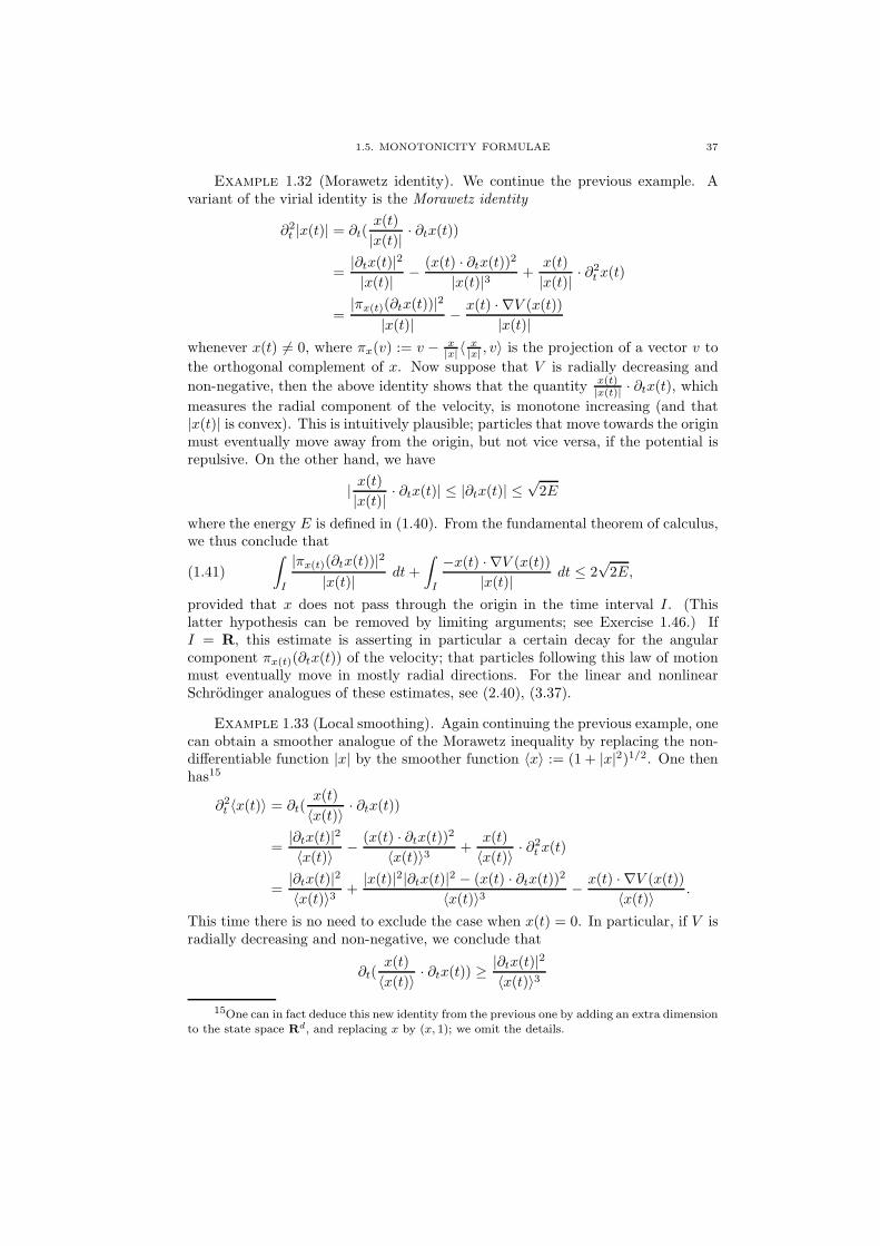
1.5. MONOTONICITY FORMULAE 37
Example 1.32 (Morawetz identity). We continue the previous example. Avariant of the virial identity is the Morawetz identity
∂2t |x(t)| = ∂t(
x(t)
|x(t)| · ∂tx(t))
=|∂tx(t)|2|x(t)| − (x(t) · ∂tx(t))2
|x(t)|3 +x(t)
|x(t)| · ∂2t x(t)
=|πx(t)(∂tx(t))|2
|x(t)| − x(t) · ∇V (x(t))
|x(t)|whenever x(t) 6= 0, where πx(v) := v − x
|x|〈 x|x| , v〉 is the projection of a vector v to
the orthogonal complement of x. Now suppose that V is radially decreasing and
non-negative, then the above identity shows that the quantity x(t)|x(t)| · ∂tx(t), which
measures the radial component of the velocity, is monotone increasing (and that|x(t)| is convex). This is intuitively plausible; particles that move towards the originmust eventually move away from the origin, but not vice versa, if the potential isrepulsive. On the other hand, we have
| x(t)|x(t)| · ∂tx(t)| ≤ |∂tx(t)| ≤√
2E
where the energy E is defined in (1.40). From the fundamental theorem of calculus,we thus conclude that
(1.41)
∫
I
|πx(t)(∂tx(t))|2|x(t)| dt+
∫
I
−x(t) · ∇V (x(t))
|x(t)| dt ≤ 2√
2E,
provided that x does not pass through the origin in the time interval I. (Thislatter hypothesis can be removed by limiting arguments; see Exercise 1.46.) IfI = R, this estimate is asserting in particular a certain decay for the angularcomponent πx(t)(∂tx(t)) of the velocity; that particles following this law of motionmust eventually move in mostly radial directions. For the linear and nonlinearSchrodinger analogues of these estimates, see (2.40), (3.37).
Example 1.33 (Local smoothing). Again continuing the previous example, onecan obtain a smoother analogue of the Morawetz inequality by replacing the non-differentiable function |x| by the smoother function 〈x〉 := (1 + |x|2)1/2. One thenhas15
∂2t 〈x(t)〉 = ∂t(
x(t)
〈x(t)〉 · ∂tx(t))
=|∂tx(t)|2〈x(t)〉 − (x(t) · ∂tx(t))2
〈x(t)〉3 +x(t)
〈x(t)〉 · ∂2t x(t)
=|∂tx(t)|2〈x(t)〉3 +
|x(t)|2|∂tx(t)|2 − (x(t) · ∂tx(t))2〈x(t)〉3 − x(t) · ∇V (x(t))
〈x(t)〉 .
This time there is no need to exclude the case when x(t) = 0. In particular, if V isradially decreasing and non-negative, we conclude that
∂t(x(t)
〈x(t)〉 · ∂tx(t)) ≥|∂tx(t)|2〈x(t)〉3
15One can in fact deduce this new identity from the previous one by adding an extra dimensionto the state space Rd, and replacing x by (x, 1); we omit the details.

38 1. ORDINARY DIFFERENTIAL EQUATIONS
x(2)
x(1)
x(3)
Figure 10. A particle passing by the origin, encountering a repul-sive force, will convert its ingoing momentum to outgoing momen-tum. Since there is no way to convert outgoing momentum backto ingoing momentum, we conclude that if the total energy (andhence momentum) is bounded, then the particle cannot move pastthe origin for extended periods of time. Note that this diagram isslightly different from the one in Figure 1 because the equation issecond-order rather than first-order in time; the position controlsthe acceleration rather than the velocity.
and hence by using the fundamental theorem of calculus we obtain the local smooth-ing estimate ∫
I
|∂tx(t)|2〈x(t)〉3 dt ≤ CE1/2
for some absolute constant C > 0. This result is perhaps a little surprising, sinceE1/2 only seems to control the speed |∂tx(t)|, as opposed to the square of the speed|∂tx(t)|2. Intuitively, the reason for this is the localisation factor 1
〈x(t)〉3 , combined
with the integration in time. When the particle x(t) is travelling at very highspeeds, then |∂tx(t)|2 is much larger than |∂tx(t)|, but to compensate for this, theparticle only lives near the origin (where the localisation factor 1
〈x(t)〉3 is large)
for a brief time. In Section 2.4, we shall quantise this estimate to Schrodingerequations; the ability to upgrade the speed to the square of the speed will becomea smoothing effect of half a derivative, which may help explain the terminology“local smoothing”.
Example 1.34 (Interaction Morawetz). Consider an N -particle system of non-interacting particles with masses m1, . . . ,mN > 0, with the classical solution x :I → (Rd)N given by Newton first law
mi∂2t xi(t) = 0 for i = 1, . . . , N.

1.5. MONOTONICITY FORMULAE 39
x (1)i
x (2)x (2)
x (1)
j
j
i
Figure 11. When two particles “collide” (i.e. pass through eachother), their mutual ingoing momentum is converted to mutualoutgoing momentum. As there is no mechanism to convert mutualoutgoing momentum back into mutual ingoing momentum, we thussee that the total number of collisions (weighted by their mass andrelative velocity) is controlled by the total momentum.
It is easily verified that this system has a conserved energy
E :=∑
i
1
2mi|∂txi(t)|2
and one trivially also has a conserved mass M :=∑
imi. Let define a collisionto be a triplet (i, j, t) where t is a time and 1 ≤ i < j ≤ N are indices such thatxi(t) = xj(t). Let us make the assumption that only finitely many collisions occurin the time interval I. If t is not one of the times where a collision occurs, we candefine the interaction momentum
P (t) :=∑ ∑
1≤i<j≤Nmimj
xi(t) − xj(t)
|xi(t) − xj(t)|· ∂t(xi(t) − xj(t));
roughly speaking, this measures how much the particles are receding from eachother. A computation shows that
∂tP (t) =∑ ∑
1≤i<j≤Nmimj
|πxi(t)−xj(t)∂t(xi(t) − xj(t))|2|xi(t) − xj(t)|
≥ 0
when t is not a collision time. Each collision (i, j, t) causes a jump in P (t) by2mimj |∂t(xi(t) − xj(t))|, thus P is monotone increasing. Using the crude bound
|P (t)| ≤∑
i
mi
∑
j
mj|∂txj(t)| ≤M√
2ME
from Cauchy-Schwarz, we thus conclude the interaction Morawetz inequality∑
(i,j,t)
2mimj |∂t(xi(t) − xj(t))| ≤ 2M√
2ME
where (i, j, t) runs over all collisions. There is a related (though not completelyanalogous) inequality for the nonlinear Schrodinger equation; see (3.42).

40 1. ORDINARY DIFFERENTIAL EQUATIONS
Exercise 1.46. Let V : Rd → R be twice continuously differentiable, radiallydecreasing (so in particular ∇V (0) = 0), and non-negative, and let u0 ∈ Rd. Showthat there is a unique global solution u : R → Rd to (1.39) with initial datumu(0) = u0. Also, show that if x(t) is not identically zero, then x(t) can equal zerofor at most one time t0 ∈ R, and in such a case we can refine (1.41) to
∫
R
|πx(t)(∂tx(t))|2|x(t)| dt+
∫
R
−x(t) · ∇V (x(t))
|x(t)| dt+ 2|∂tx(t0)| ≤ 2√
2E.
Exercise 1.47. With the same hypotheses as Exercise 1.46, show that for eachε > 0 we have the estimate ∫
R
|∂tx(t)|2〈x(t)〉1+ε dt .ε E
1/2.
This improves upon Example 1.33, which dealt with the case ε = 2. (Hint: use themonotonicity formulae already established, as well as some new formulae obtainedby considering derivatives of expressions such as 〈x(t)〉−1−ε(x(t) · ∂tx(t)).) Showthat the estimate fails at the endpoint ε = 0, even when V = 0 (compare this with(1.41)).
Exercise 1.48 (Virial identity). Suppose that x1, . . . , xN ∈ C2loc(R → Rd) are
solutions to the system of ODE
mj∂2t xj(t) = −
∑
i6=jG
mimj
|xi(t) − xj(t)|2xj(t) − xi(t)
|xj(t) − xi(t)|
where the masses m1, . . . ,mN are positive, and G > 0 is an absolute constant; thismodels the behaviour of N particles under Newtonian gravity. Assume that the xjare all uniformly bounded in time and that |xi − xj | never vanishes for any i 6= j.Suppose also that the average kinetic and potential energies
K := limT→+∞
1
2T
∫ T
−T
N∑
j=1
1
2mj |∂txj(t)|2 dt;
V := limT→+∞
− 1
2T
∫ T
−T
∑
1≤i<j≤N
Gmimj
|xi(t) − xj(t)|dt
exist. Conclude the virial identity K = − 12T . (Hint: look at Example 1.31.) This
identity is of importance in astrophysics, as it allows one to infer the potentialenergy (and hence the possible existence of dark matter) from measurements of thekinetic energy (e.g. via red-shift measurements).
1.6. Linear and semilinear equations
Mathematics would certainly have not come into existence if onehad known from the beginning that there was in nature no exactlystraight line, no actual circle, no absolute magnitude. (FriedrichNietzsche, “Human, All Too Human”)
Let us now return to the general Cauchy problem (1.7). We shall assume thatwe have a special solution, the vacuum solution u(t) ≡ 0; in other words, we assumethat F (0) = 0. If F is continuously differentiable, we can then perform a Taylorexpansion
F (u) = Lu+N(u)
1.6. LINEAR AND SEMILINEAR EQUATIONS 41
where L ∈ End(D) is a linear operator, and N : D → D vanishes faster than linearlyat 0, thus
(1.42) lim‖u‖D→0
N(‖u‖D)
‖u‖D= 0.
We shall refer to L as the linear component of F , and N as the genuinely nonlinearcomponent. Thus we can write our quasilinear equation as a semilinear equation16
(1.43) ∂tu(t) − Lu(t) = N(u(t)).
If N = 0, we say that the equation is linear, otherwise it is nonlinear. In general,linear equations are much better understood than nonlinear equations, as a vastarray of tools such as linear algebra, spectral theory, Fourier analysis, special func-tions (explicit solutions), and the principle of superposition can be now invoked toanalyze the equation. A very profitable idea in solving equations such as (1.43) isto treat the genuine nonlinearity N(u) as negligible, and thus to view the equation(1.43) as a perturbation of the linear equation
(1.44) ∂tu(t) − Lu(t) = 0.
This perturbation strategy is reasonable if u is small (so that N(u), which vanishesto at least second order, will be very small compared to Lu) or if one is only solvingthe equation for very short times (so that the nonlinearity does not have much ofa cumulative influence on the solution). However, when considering large solutionsfor long periods of time, the perturbation approach usually needs to be abandonedin favour more “global” or “non-perturbative” techniques such as energy methodsor monotonicity formula methods, although if one establishes a sufficient amountof decay on the solution in time, then one can often re-instate the perturbationanalysis in the asymptotic limit t→ ∞, which can be used for instance to obtain ascattering theory.
In accordance to this perturbation philosophy, let us study (1.43) by first con-sidering the linear equation (1.44), say with initial datum u(0) = u0 ∈ D. (We knowfrom time translation invariance that the choice of initial time t0 is not particularlyrelevant.) Then there is a unique global solution to (1.44), given by
u(t) = etLu0 =∞∑
n=0
tn
n!Lnu0;
the finite dimensionality of D ensures that L is bounded, and hence this sum isabsolutely convergent. We refer to the linear operators etL ∈ End(D) as the linearpropagators ; observe that we have the group law etLesL = e(t+s)L with e0L = id.In particular, if u0 is an eigenvector of L, thus Lu0 = λu0 for some λ ∈ C, thenthe unique global solution to (1.44) is given by u(t) = etλu0.
It is thus clear that the eigenvalues of L will play an important role in theevolution of the equation (1.44). If L has eigenvalues with negative real part, thenthe equation is stable or dissipative in the corresponding eigenspaces, displayingexponential decay in time as t → +∞ (but exponential growth as t → −∞).Conversely, if L has eigenvalues with positive real part, then the equation is unstable
16For ODE, there is little distinction between a quasilinear equation and a semilinear one.For PDE, one usually requires in a semilinear equation that the genuinely nonlinear part N(u) ofthe equation is lower order (i.e. involves fewer spatial derivatives) than the linear part Lu; someauthors require that N(u) contain no derivatives whatsoever.
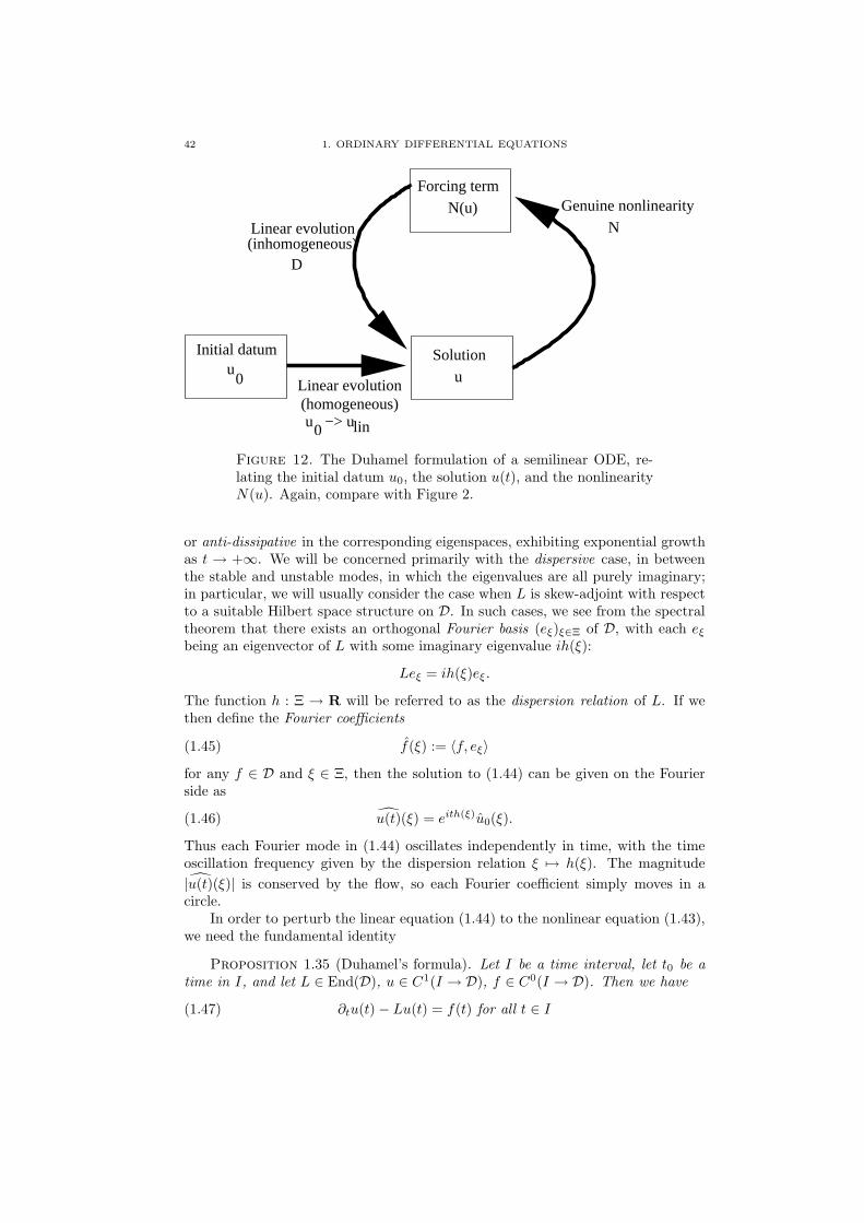
42 1. ORDINARY DIFFERENTIAL EQUATIONS
D
u −> u0 lin
Forcing term
Solutionuu
0
Initial datum
(homogeneous)Linear evolution
(inhomogeneous)Linear evolution
N(u) Genuine nonlinearity N
Figure 12. The Duhamel formulation of a semilinear ODE, re-lating the initial datum u0, the solution u(t), and the nonlinearityN(u). Again, compare with Figure 2.
or anti-dissipative in the corresponding eigenspaces, exhibiting exponential growthas t → +∞. We will be concerned primarily with the dispersive case, in betweenthe stable and unstable modes, in which the eigenvalues are all purely imaginary;in particular, we will usually consider the case when L is skew-adjoint with respectto a suitable Hilbert space structure on D. In such cases, we see from the spectraltheorem that there exists an orthogonal Fourier basis (eξ)ξ∈Ξ of D, with each eξbeing an eigenvector of L with some imaginary eigenvalue ih(ξ):
Leξ = ih(ξ)eξ.
The function h : Ξ → R will be referred to as the dispersion relation of L. If wethen define the Fourier coefficients
(1.45) f(ξ) := 〈f, eξ〉for any f ∈ D and ξ ∈ Ξ, then the solution to (1.44) can be given on the Fourierside as
(1.46) u(t)(ξ) = eith(ξ)u0(ξ).
Thus each Fourier mode in (1.44) oscillates independently in time, with the timeoscillation frequency given by the dispersion relation ξ 7→ h(ξ). The magnitude
|u(t)(ξ)| is conserved by the flow, so each Fourier coefficient simply moves in acircle.
In order to perturb the linear equation (1.44) to the nonlinear equation (1.43),we need the fundamental identity
Proposition 1.35 (Duhamel’s formula). Let I be a time interval, let t0 be atime in I, and let L ∈ End(D), u ∈ C1(I → D), f ∈ C0(I → D). Then we have
(1.47) ∂tu(t) − Lu(t) = f(t) for all t ∈ I

1.6. LINEAR AND SEMILINEAR EQUATIONS 43
if and only if
(1.48) u(t) = e(t−t0)Lu(t0) +
∫ t
t0
e(t−s)Lf(s) ds for all t ∈ I,
where we adopt the convention that∫ tt0
= −∫ t0t
if t < t0.
Remark 1.36. The case L = 0 is just the fundamental theorem of calculus.Indeed one can view Duhamel’s formula as the fundamental theorem of calculus,twisted (i.e. conjugated) by the linear propagator etL; this helps explain the simi-larity between Figure 2 and Figure 12.
Proof. If we make the ansatz17 u(t) = etLv(t) for some v : I → D in (1.47),then (1.47) is equivalent to
∂tv(t) = e−tLf(t),
which by the fundamental theorem of calculus is equivalent to
v(t) = v(t0) +
∫ t
t0
e−sLf(s) ds.
The claim then follows by multiplying both sides by etL and using the group law.
In view of this proposition, we see that if N : D → D is continuous and u isassumed to be continuous, then the Cauchy problem
∂tu− Lu = N(u); u(0) = u0,
is equivalent to the integral equation
(1.49) u(t) = etLu0 +
∫ t
0
e(t−s)LN(u(s)) ds.
This should be compared with the solution u(t) = etLu0 of the corresponding linearproblem; thus if we think of N as being small, (1.49) is a quantitative formulationof the assertion that the nonlinear solution resembles the linear solution. One canview (1.49) as the strong solution concept for u, adapted to the flow etL of thelinear operator L.
The equation (1.49) is a variant of (1.8), but is a little “smarter” in that it usesthe more accurate approximation etLu0 to the nonlinear solution u, as opposed tothe somewhat cruder approximation u0. As a consequence, the error term in (1.49)tends to be somewhat smaller than that in (1.8), as it involves just the genuinelynonlinear component N of the nonlinearity. Just as (1.8) can be iterated using thecontraction mapping theorem to obtain the Picard existence theorem, the variant(1.49) can also be iterated to obtain a variant of the Picard existence theorem,which can exploit the special properties of the linear propagator etL to give betterbounds on the time of existence. To describe this iteration scheme, let us first workabstractly, viewing (1.49) as instance of the more general equation
(1.50) u = ulin +DN(u)
17This is of course the technique of integrating factors, which is a special case of the methodof variation of parameters. The choice of ansatz u(t) = etLv(t) is inspired by the fact that onesolves the linear equation (1.44) if and only if v is constant.

44 1. ORDINARY DIFFERENTIAL EQUATIONS
Forcing term
Solution
Genuine nonlinearity N
Linear solutionu
linu0
in Du
N(u) in N
in Bin Bε/2
Lose C0Gain 1 / 2C0
ε
Duhamel operatorD
Initial datum
Figure 13. The iteration scheme for Proposition 1.38. In prac-tice, the object ulin arises as the linear evolution of some initialdatum u0, as in Figure 12, though we do not use this in the state-ment and proof of the Proposition.
where ulin(t) := etLu0 is the linear solution, and D is the Duhamel operator
DF (t) :=
∫ t
0
e(t−s)LF (s) ds.
A useful heuristic principle in trying to solve equations of this general abstract typeis
Principle 1.37 (Perturbation principle). If one is working on a time interval[0, T ] such that DN(u) ≪ ulin, then u should evolve on [0, T ] as if it were linear(in particular, the solution should exist and obey the same type of estimates thatulin does). If one is working instead on a time interval where DN(u) ≫ ulin, oneshould expect u to exhibit nonlinear behaviour (which could range from blowup orexcessive growth on one hand, to additional decay on the other, or something inbetween such as nontrivial nonlinear oscillation).
This is of course a very vague principle, since terms such as “≪”, “≫”, or“nonlinear behaviour” are not well defined. In practice, DN(u) will tend to besmall compared to ulin if the initial datum u0 is suitably small, or if the time t isclose to 0, so for small data or small times one expects linear-type behaviour. Forlarge data or large times, perturbation theory does not predict linear behaviour,and one could now have nonlinear effects such as blowup18. To control solutionsin this regime one generally needs to augment the perturbation theory with othertools such as conservation laws.
Let us now give a rigorous formulation of the first half of this principle, by usingthe following variant of the contraction mapping theorem to construct solutions.
18Note however that it is possible for the nonlinear term to dominate the linear term butstill be able to construct and control solutions. This for instance occurs if there is an “energycancellation” that shows that the nonlinear term, while nominally stronger than the linear term,is somehow “almost orthogonal” to the solution in the sense that it does not significantly increase
certain energies; we shall see several examples of this in the text. Thus the solutions will notstay close to the linear solution but will still be bounded in various norms. In certain defocusingdissipative settings it is even possible for the nonlinearity to always act to reduce the energy, thusgiving a better behaved solution than the linear equation.

1.6. LINEAR AND SEMILINEAR EQUATIONS 45
Proposition 1.38 (Abstract iteration argument). Let N , S be two Banachspaces. Suppose we are given a linear operator D : N → S with the bound
(1.51) ‖DF‖S ≤ C0‖F‖Nfor all F ∈ N and some C0 > 0, and suppose that we are given a nonlinear operatorN : S → N with N(0) = 0, which obeys the Lipschitz bounds
‖N(u) −N(v)‖N ≤ 1
2C0‖u− v‖S(1.52)
for all u, v in the ball Bε := u ∈ S : ‖u‖S ≤ ε, for some ε > 0. (In other words,‖N‖C0,1(Bε→N ) ≤ 1
2C0.) Then for all ulin ∈ Bε/2 there exists a unique solution
u ∈ Bε to the equation (1.50), with the map ulin 7→ u Lipschitz with constant atmost 2. In particular we have
(1.53) ‖u‖S ≤ 2‖ulin‖S .This proposition is established by the arguments used to prove the contraction
mapping principle, and is left as an exercise. The idea of using this type of abstractDuhamel iteration to tackle nonlinear PDE dates back to [Seg].
Remarks 1.39. Note that we have considerable freedom in selecting the spacesS and N ; this freedom becomes very important when considering the low-regularitylocal wellposedness theory of PDE. The Picard existence argument in Theorem 1.7corresponds, roughly speaking, to the choice S = N = C0(I → D), with (1.8)taking the place of (1.49). There are a number of variations of this iteration scheme;for instance, instead of measuring the solution u in a single norm S, one sometimesis in a situation where u is measured both in a “smooth” norm S and a “rough”norm S0; the solution may be large in the smooth norm but small in the rough norm.In such cases it can still be possible to close an iteration argument using estimatesthat combine both norms together; this becomes important in the large data theoryand in the persistence of regularity theory. While it is possible to build an abstractframework for such schemes, the formulation becomes rather complicated, and sowhen these types of situations arise (see for instance Proposition 3.11) we shallsimply perform the iteration by hand.
Remark 1.40. As with Remark 1.5, the proof of the above theorem providesan explicit iteration scheme to construct the desired solution, starting with thelinear iterate u(0) := ulin and then constructing successive Duhamel iterates u(n) :=ulin + DN(u(n−1)). This scheme often converges better than the one in Remark1.5, though it is far from the most rapidly convergent scheme (and is usually notused directly in numerical computations).
We illustrate the iteration method by establishing global existence for linearlystable nonlinear equations from small data.
Proposition 1.41 (Linear stability implies nonlinear stability). Let D be afinite-dimensional real Hilbert space, and let L ∈ End(D) be a linear operator whichis linearly stable in the sense that19 there exists σ > 0 such that 〈Lu, u〉 ≤ −σ‖u‖2
D
19In the finite-dimensional case, linear stability is equivalent to the spectrum of L being
contained entirely in the interior of the left half-plane. In the infinite-dimensional case, therelationship between stability and spectrum is more delicate, especially if L fails to be normal orself-adjoint. Indeed, for PDE, nonlinear stability is often significantly more difficult to establishthan linear stability.

46 1. ORDINARY DIFFERENTIAL EQUATIONS
u(t)
L u(t)
N(u(t))
Figure 14. Proposition 1.41 from the vector field perspective ofFigure 1. If u is sufficiently small, then the dissipative effect ofthe linear term Lu will dominate the effect of the nonlinearityN(u), regardless of the orientation of N(u), causing u to decayexponentially towards the origin.
for all u ∈ D. Let N ∈ C2loc(D → D) be a function which vanishes to more than
first order at the origin in the sense of (1.42) (in fact, the C2 hypothesis showsthat N will vanish to second order). If u0 ∈ D is sufficiently close to the origin,there exists a unique classical solution u : [0,+∞) → D to (1.43) with initial datumu(0) = u0, and furthermore there is an estimate of the form
(1.54) ‖u(t)‖D ≤ 2e−σt‖u0‖D.Proof. The uniqueness of u follows from the Picard uniqueness theorem, so
it suffices to establish existence, as well as the estimate (1.54). A simple Gronwallargument (see Exercise 1.54) gives the dissipative estimate
(1.55) ‖etLu0‖D ≤ e−σt‖u0‖Dfor all u0 ∈ D and t ≥ 0. Let us now define the spaces S to be the space of allfunctions u ∈ C0([0,+∞) → D) whose norm
‖u‖S := supt≥0
eσt‖u(t)‖D
is finite, and let N be the space of all functions F ∈ C0([0,+∞) → D) then
‖u‖N := supt≥0
eσt‖u(t)‖D
is finite. Thus if we set ulin(t) := etLu0 then ‖ulin‖S ≤ ‖u0‖D. Next, observe from(1.42) that ∇N(0) = 0, and so by Taylor expansion and the hypothesis that N isC2, we have ∇N(u) = ON (‖u‖D) for ‖u‖D sufficiently small (the implied constantdepends of course on N). From the fundamental theorem of calculus this impliesthat
‖N(u) −N(v)‖D ≪N ‖u− v‖D(‖u‖D + ‖v‖D)
1.6. LINEAR AND SEMILINEAR EQUATIONS 47
whenever ‖u‖D, ‖v‖D are sufficiently small. In particular, if ‖u‖S, ‖v‖S ≤ ε forsome sufficiently small ε, then we have
‖N(u(t)) −N(v(t))‖D ≪N e−σt‖u− v‖Sεe−σt
and hence (if ε is sufficiently small)
‖N(u) −N(v)‖N ≤ 1
2σ‖u− v‖S .
whenever ‖u‖S , ‖v‖S ≤ ε. Also, from the triangle inequality and (1.55) we have
‖DF‖S ≤ 1
σ‖F‖N
where D is the Duhamel operator. From Proposition 1.38 we thus see that if‖u0‖D ≤ ε/2, then can thus construct a solution u to (1.47) with ‖u‖S ≤ 2‖ulin‖S ≤2‖u0‖D, and the claim follows.
Remark 1.42. If one merely assumes N to be Lipschitz rather than C2loc,
then one can obtain some weaker decay estimates, for instance given any σ′ < σone can obtain an estimate ‖u(t)‖D ≤ 2e−σ
′t‖u0‖D if ‖u0‖D is sufficiently smalldepending on N and σ, σ′. This can be achieved for instance by modifying theGronwall inequality argument in Exercise 1.54. We leave the details to the readeras an exercise. Thus for dissipative equations one often has the luxury of concedingan exponential factor in the time variable t, which is very helpful for keeping theiteration under control. When we turn to nonlinear dispersive equations, no suchexponential factors are available for us to concede (although in some cases thedispersion will give us polynomial type decay in t, which can be quite useful), andwe must proceed with a bit more care.
An important special case of the general equation (1.43) occurs when the gen-uinely nonlinear component N is k-linear for some k ≥ 2, in the sense that
N(u) = Nk(u, u, . . . , u)
where Nk : Xk → X is a function which is (real-)linear in each of the k variables.In the k = 2 case we call N bilinear or quadratic, in the k = 3 case we call Ntrilinear or cubic, and so forth. The condition k ≥ 2 is essentially forced upon usby the condition (1.42). In these cases, the hypothesis (1.52) will hold for ε smallprovided that N is bounded from S to N ; see Exercise 1.51.
When the nonlinearity is k-linear and the linear term L is skew-adjoint, onecan view the evolution (1.43) in terms of frequency interactions (using the “Fouriertransform” (1.45)). We illustrate this in the k = 2 caseN(u) = N2(u, u); to simplifythe exposition, we will also assume that N2 is not only real linear but is in factcomplex linear. The situation for antilinear nonlinearities and for higher ordersk > 2 requires some simple modifications to the discussion below which are left tothe reader. If we take Fourier transforms of (1.49) (using (1.46)), we obtain
u(t)(ξ) = eith(ξ)u0(ξ) +
∫ t
0
ei(t−s)h(ξ)∑
ξ1,ξ2
cξ1,ξ2ξ u(s)(ξ1)u(s)(ξ2) ds
where cξ1,ξ2ξ is the structure constant
cξ1,ξ2ξ := 〈N2(eξ1 , eξ2), eξ〉.

48 1. ORDINARY DIFFERENTIAL EQUATIONS
Typically, the structure constants will usually be zero; given any mode ξ, only afew pairs of modes ξ1, ξ2 can interact to excite that mode; a typical constraint
in order for cξ1,ξ2ξ to be non-zero is of the form ξ = ξ1 + ξ2 (where one places
some group structure on the space Ξ of frequencies). Making the renormalisation
u(t)(ξ) := eith(ξ)aξ(t), which is suggested to us by the variation of parametersmethod, we obtain an integral system of equations for the functions (aξ(t))ξ∈Ξ:
(1.56) aξ(t) = u0(ξ) +
∫ t
0
eis(h(ξ1)+h(ξ2)−h(ξ))cξ1,ξ2ξ aξ1(s)aξ2(s) ds.
Thus each aξ(t) is initially set equal to u0(ξ), but as time evolves, the ξ-modesaξ(t) is influenced by the bilinear interactions of the pairs of modes aξ1(t), aξ2(t)that can excite the ξ-mode. The resonance function h(ξ1) + h(ξ2) − h(ξ) plays akey role in the analysis. If this quantity is large in magnitude, then the integral in(1.56) will be highly oscillatory, and thus likely to be rather small; in this case, wesay that the interaction between the modes ξ1, ξ2, ξ is non-resonant. The dominantcontribution to (1.56) typically consists instead of the resonant interactions, inwhich the resonance function is zero or small. In order to obtain an iterativescheme for solving this equation (using for instance Proposition 1.38), especially atlow regularities, one often has to spend some effort to control the resonant portionsof interaction, either by showing that the resonant interactions are fairly rare, or
by extracting some “null structure” from the structure coefficients cξ1,ξ2ξ , whichcauses them to vanish whenever the resonance function vanishes. We will see someexamples of this in later sections.
Exercise 1.49. Prove Proposition 1.38. (Hint: review the proof of Theorem1.4, Theorem 1.7, and Exercise 1.2.)
Exercise 1.50 (Stability). Let the notation and hypotheses be as in Proposi-tion 1.38. Suppose that ulin ∈ Bε/2, and we have an approximate solution u ∈ Bεto the equation (1.50), in the sense that u = ulin +DN(u) + e for some e ∈ S. Letu ∈ Bε be the actual solution to (1.50) given by the above Proposition. Show that‖u − u‖S ≤ 2‖e‖S . Note that this generalises the Lipschitz claim in Proposition1.38.
Exercise 1.51. Let N ,S be Banach spaces as in Proposition 1.38, and supposethat one is given a k-linear nonlinearity N(u) = Nk(u, . . . , u), which maps S to Nwith the k-linear estimate
‖N(u1, . . . , uk)‖N ≤ C1‖u1‖S . . . ‖uk‖Sfor all u1, . . . , uk ∈ S and some constant C1 > 0. Show that the hypothesis (1.52)holds for u, v ∈ Bε with ε := 1
2kC0C1.
Exercise 1.52 (Second order Duhamel). Let L ∈ End(D). Show that thesolution to the homogeneous linear second-order ODE
∂ttu− Lu = 0
with initial datum u(0) = u0, ∂tu(0) = u1 is given by u(t) = U0(t)u0 + U1(t)u1 forsome operators U0 : R ×D → D, U1 : R ×D → D. Show that the unique classicalsolution u ∈ C2
loc(D → R) to the inhomogeneous linear second-order ODE
∂ttu− Lu = f

1.7. COMPLETELY INTEGRABLE SYSTEMS 49
with initial datum u(t0) = u0, ∂tu(t0) = u1, where f ∈ C0loc(D → D) and t0 ∈ R,
is given by the Duhamel formula
u(t) = U0(t− t0)u0 + U1(t− t0)u1 +
∫ t
t0
U1(t− s)f(s) ds.
(Hint: convert the second-order equation to a first order one, then use Proposition1.35.)
Exercise 1.53 (Duhamel vs. resolvents). Let L, V, L0 ∈ End(D) be such thatL = L0 + V . Use Duhamel’s formula to show that
etL = etL0 +
∫ t
0
e(t−s)L0V esL ds = etL0 +
∫ t
0
e(t−s)LV esL0 ds.
If λ is a scalar such that the resolvent operators R(λ) := (L − λ)−1 and R0(λ) :=(L0 − λ)−1 exist, establish the resolvent identity
R(λ) = R0(λ) −R0(λ)V R(λ) = R0(λ) −R(λ)V R0(λ)
and discuss the relationship between the above identities using the Fourier dualitybetween t and λ.
Exercise 1.54. Let L be as in Proposition 1.41, and let u solve the equation(1.44). Use Gronwall’s inequality to establish the bound ‖u(t)‖D ≤ e−σt‖u(0)‖Dfor all t ≥ 0. (Hint: establish a monotonicity formula for ‖u(t)‖2
D, and then use theversion of Gronwall’s inequality mentioned in Exercise 1.7.)
Exercise 1.55 (Stable manifold). Let D be a finite-dimensional real Hilbertspace, and let L ∈ End(D) be weakly linearly stable in the sense that 〈Lu, u〉 ≤ 0
for all u ∈ D. Let N ∈ C0,1loc (D → D) have the property that 〈N(u), u〉 ≤ 0
for all u ∈ D. Show that for any u0 ∈ D, there exists a unique classical solutionu : [0,+∞) → D to (1.43) with initial datum u(0) = u0, which is uniformly boundedand obeys the estimate
∫ ∞
0
|〈Lu(t), u(t)〉| dt ≤ ‖u0‖2D.
Conclude in particular that if V is the subspace V := u ∈ D : 〈Lu, u〉 = 0, thatdist(u(t), V ) → 0 as t→ +∞.
1.7. Completely integrable systems
Tyger! Tyger! burning brightIn the forests of the night,What immortal hand or eyeCould frame thy fearful symmetry?(William Blake, “The Tyger”)
We have already encountered Hamiltonian ODE in Section 1.4, which enjoyat least one conserved integral of motion, namely the Hamiltonian H itself. Thisconstrains the Hamiltonian flow to a codimension one subspace of the symplecticphase space D. Additional conserved integrals of motion can constrain the flowfurther. It turns out that the largest number of independent conserved integrals thatone can have in a Hamiltonian system is half the dimension of the phase space (see

50 1. ORDINARY DIFFERENTIAL EQUATIONS
Exercise 1.56). When this occurs, we say that the system is completely integrable20;the phase space splits completely into the conserved quantities E1, . . . , EN (alsocalled action variables), together with the dynamic variables (also called anglevariables) induced by the N flows corresponding to E1, . . . , EN .
Example 1.43 (Simple harmonic oscillator). Let D = Cn be the phase space inExample 1.28, and let H be the Hamiltonian (1.32). Then there are n independentconserved quantities
E1 := |z1|2; . . . ;En := |zn|2
and n angle variables θ1, . . . , θn ∈ T, defined for most points in phase space bypolar coordinates
z1 = |z1|eiθ1 ; . . . ; zn = |zn|eiθn .
Then the Hamiltonian flow in these action-angle coordinates becomes linear:
∂jEj(t) = 0; ∂jθj(t) = λj .
Also, observe that the Hamiltonian H is just a linear combination of the basicconserved quantities E1, . . . , En, which is of course consistent with the fact that His itself conserved. More generally, any linear system (1.44) in which L is skew-adjoint will lead to a completely integrable system.
There are many ways to determine if a system is completely integrable. Weshall discuss only one, the method of Lax pairs.
Definition 1.44. Consider an ODE
(1.57) ∂tu(t) = F (u(t)),
where F ∈ C0,1loc (D → D) and D is a finite-dimensional phase space. Let H be a
finite-dimensional complex Hilbert space, and let End(H) be the space of linearmaps from H to itself (for instance, if H = Cn, then End(H) is essentially the ringof n × n complex matrices). A Lax pair for the ODE (1.57) is any pair L,P ∈C1
loc(D → End(H)) of functions such that we have the identity
(1.58) ∂tL(u(t)) = [L(u(t)), P (u(t))]
for all classical solutions u : I → D to the ODE (1.57), or equivalently if
(F (u) · ∇)L(u) = [L(u), P (u)] for all u ∈ D.Here [A,B] := AB −BA denotes the usual Lie bracket of the matrices A and B.
Remark 1.45. Geometrically, (1.58) asserts that the matrix L(u(t)) evolvesvia “infinitesimal rotations” that are “orthogonal” to L(u(t)). In many cases, Pwill take values in the Lie algebra g of some Lie group G in End(H), and L willtake values either in the Lie algebra g or the Lie group G; note that the equation(1.58) is consistent with this assumption, since Lie algebras are always closed underthe Lie bracket (see also Exercise 1.15).
20This definition unfortunately does not rigorously extend to the infinite dimensional phase
spaces one encounters in PDE. Indeed, we do not yet have a fully satisfactory definition of whatit means for a PDE to be completely integrable, though we can certainly identify certain verysuggestive “symptoms” of complete integrability of a PDE, such as the presence of infinitely manyconserved quantities, a Lax pair formulation, or the existence of explicit multisoliton solutions.

1.7. COMPLETELY INTEGRABLE SYSTEMS 51
A trivial example of a Lax pair is when L : D → Mn(C) is constant, and Pis chosen to commute with L; we shall be more interested in non-trivial exampleswhen L, and more precisely the spectrum (eigenvalues) of L, admit some genuinevariation across the phase space D. A simple example is provided by the one-dimensional harmonic oscillator
∂tu = iωu
in the phase space D = C, with H = C2 and Lax pair
(1.59) L(u) :=
(i(|u|2 − λ) iu2
iu2 i(λ− |u|2)
); P (u) :=
(−iω 00 iω
)
where the spectral parameter λ is an arbitrary complex number. Here, L and P takevalues in the Lie algebra su2(C) of SU2(C), the group of 2 × 2 unitary matrices.The higher-dimensional harmonic oscillator in Example 1.28 can also be given aLax pair by taking direct sums of the above example; we omit the details.
Now we show how Lax pairs lead to conserved quantities.
Proposition 1.46. Suppose that an ODE (1.57) is endowed with a Lax pairL : D → End(H), P : D → End(H). Then for any non-negative integer k, themoment tr(Lk) is preserved by the flow (1.57), as is the spectrum σ(L) := λ ∈ C :L− λ not invertible.
Proof. We begin with the moments tr(Lk). Let u : I → D solve (1.57). Fromthe Leibnitz rule and the first trace identity
(1.60) tr(AB) = tr(BA)
we have
∂ttr(L(u(t))k) = ktr(L(u(t))k−1∂tL(u(t))) = ktr(L(u(t))k−1[L(u(t)), P (u(t))]).
But from the second trace identity
(1.61) tr(A[B,C]) = tr(B[C,A]) = tr(C[A,B])
(which follows easily from the first trace identity), and the obvious fact that Lk−1
commutes with L, we obtain ∂ttr(L(u(t))k) = 0 as desired.One can conclude conservation of the spectrum σ(L) from that of the moments
by using the characteristic polynomial of L. For a more direct approach (whichdoes not rely as much on the finite dimensionality of L), see Exercise 1.57.
The quantities tr(L), tr(L2), . . . may seem like an infinite number of conservedquantities, but they are of course not all independent. For instance in the example(1.59), all the quantities tr(Lk) are functions of a single conserved quantity |z|2.This makes the number of conserved quantities equal to the half the (real) dimensionof the phase space C, and so this equation is completely integrable.
One special case of solutions to a completely integrable system arises when thespectrum σ(L) of the Lax operator is unexpectedly simple, for instance if L is arank one operator. This often leads to very algebraically structured solutions suchas solitary waves (solitons). For instance, in Example 1.43, the case when L isrank one corresponds to that of a single excited mode, when only one of the zj isnon-zero, which can be viewed as a rather trivial instance of a solitary wave. Themore general task of reconstructing the solution given the spectral information onL (and certain supplemental “scattering data” associated to the initial datum u0)is known as inverse scattering and is a very rich subject involving some beautiful

52 1. ORDINARY DIFFERENTIAL EQUATIONS
analysis, algebra, and geometry. It is well outside the scope of this monograph; werefer the reader to [HSW] for an introduction.
We now give some non-trivial examples of completely integrable systems. Thefirst is the periodic Toda lattice
(1.62) ∂tan = an(bn+1 − bn); ∂tbn = 2(a2n − a2
n−1)
where n ranges over a cyclic group Z/NZ, and an : R → R, bn : R → R are real-valued functions of time; this can be viewed as a discrete version of the periodicKorteweg-de Vries (KdV) equation. To place this lattice in Lax pair form, we let Hbe an N -dimensional real Hilbert space with orthonormal basis en : n ∈ Z/NZ,and for any given state u = ((an, bn))n∈Z/NZ we define L = L(u) : H → H andP = P (u) : H → H on basis vectors by
Len := anen+1 + bnen + an−1en−1
Pen := anen+1 − an−1en−1.
One can easily verify the Lax pair equation (1.58) by testing it on basis vectors.Note that L is self-adjoint and P is skew-adjoint, which is of course consistent with(1.58). The Toda lattice enjoys N independent conserved quantities arising fromL, including the trace
tr(L) =∑
n∈Z/NZ
bn
and the second moment
tr(L2) =∑
n∈Z/NZ
b2n + 2a2n;
one may verify by hand that these quantities are indeed preserved by (1.62). Theequation (1.62) is not a Hamiltonian flow using the standard symplectic form onthe state space, but can be transformed into a Hamiltonian flow (with Hamiltonian2tr(L2)) after a change of variables, see Exercise 1.59. One can create higher orderToda flows by using higher moments of L as Hamiltonians, but we will not pursuethis here.
Another example of a completely integrable system is the periodic Ablowitz-Ladik system
(1.63) ∂tFn = i(1 − |Fn|2)(Fn−1 + Fn+1),
where n ranges over a cyclic group Z/NZ, and Fn : R → C are complex-valuedfunctions of time with |Fn| < 1 for all n (this property is preserved by the flow).This is a discrete analogue of the cubic defocusing periodic nonlinear Schrodingerequation. To define a Lax pair (L,P ) for this equation, we take H to be a complexHilbert space spanned by 2N orthonormal basis vectors vn, wn : n ∈ Z/NZ. TheLax operator L = L(F ) : H → H is then defined on basis elements by
Lvn :=√
1 − |Fn|2vn+1 + Fnwn
Lwn+1 := −Fnvn+1 +√
1 − |Fn|2wn+1;

1.7. COMPLETELY INTEGRABLE SYSTEMS 53
note that L is in fact a unitary operator (a discrete analogue of a Dirac operator),with adjoint L∗ = L−1 given by
L∗vn+1 :=√
1 − |Fn|2vn − Fnwn+1
L∗wn := Fnvn +√
1 − |Fn|2wn+1;
The P operator is a little trickier to define. We first define the reflection operatorJ : H → H as
Jvn := vn; Jwn := −wnand then the diagonal operator D = J
8 ([L, J ]2 + [L∗, J ]2) by
Dvn :=Fn−1Fn + Fn−1Fn
2vn; Dwn := −Fn−1Fn + Fn−1Fn
2wn
and then define P by
P := i(LJL+ L∗JL∗
2−D).
The verification of (1.58) is rather tedious but straightforward. Note that P isskew-adjoint, which is consistent with (1.58) and the unitarity of L.
A completely integrable system contains some quite low-dimensional invariantsets; in many cases (as with the harmonic oscillator), these invariant sets takethe form of torii. A very interesting question concerns the stability of such in-variant surfaces; if one makes a perturbation to the Hamiltonian (destroying thecomplete integrability), does the invariant surface similarly perturb? The answercan be surprisingly subtle, involving the theory of Kolmogorov-Arnold-Moser torii,Nekhoroshev stability, and Arnold diffusion, among other things. We will not at-tempt to describe this theory here, but refer the reader to [Kuk3] for a discussionof these topics in the context of Hamiltonian PDE.
Exercise 1.56 (Lagrangian submanifolds). Call a linear subspace V of a sym-plectic phase space (D, ω) null if ω(v, v′) = 0 for all v, v′ ∈ V . Show that if V isnull, then the dimension of V cannot exceed half the dimension of D. (Hint: look atthe symplectic complement V ⊥ := u ∈ D : ω(v, u) = 0 for all v ∈ V .) Concludethat if E1, . . . , Ek are functions which Poisson commute with a given Hamilton-ian H , then for each u ∈ D the gradients ∇ωE1(u), . . . ,∇ωEk(u) span a space ofdimension at most half the dimension of D.
Exercise 1.57 (Conservation of spectrum). Let the notation and hypothesesbe as in Proposition 1.46. Suppose that for some time t0 ∈ I and some λ ∈ Lwe have λ ∈ σ(L), thus there exists a non-zero eigenvector φ0 ∈ H such thatL(u(t0))φ0 − λφ0 = 0. Now let φ : I → H solve the Cauchy problem
∂tφ(t) = P (u(t))φ(t); φ(t0) = φ0.
Show that such a solution φ exists, and furthermore we have
L(u(t))φ(t) − λφ(t) = 0
for all t ∈ I. (Hint: use Exercise 1.13). Conclude that the spectrum σ(L) is aninvariant of the flow.
Exercise 1.58 (Lax pairs vs. Hamiltonian mechanics). uppose that a sym-plectic phase space (D, ω) is endowed with maps L ∈ C1
loc(D → End(H)) andR ∈ C1
loc(D → End(End(H))). Suppose we also have the R-matrix identity
tr(AL), tr(BL) = tr(BR([L,A]) −AR([L,B]))

54 1. ORDINARY DIFFERENTIAL EQUATIONS
for all A,B ∈Mn(C), where , denotes the Poisson bracket. Conclude the Poissoncommutation relations
tr(AL), tr(Lk) = −ktr(A[L,Rt(Lk−1)])
andtr(Lm), tr(Lk) = 0
for all m, k ≥ 0 and A ∈ End(H), where Rt : D → End(End(H)) is the transposeof R, thus tr(AR(B)) = tr(BR(A)) for all A,B ∈ End(H). (Hint: take advantageof the trace identities (1.60), (1.61) and the Leibnitz rule (1.36)). Conclude thatthe Hamiltonian flows given by the Poisson-commuting Hamiltonians tr(Lk) eachhave a Lax pair (L,Pk) with Pk := −kRt(Lk−1).
Exercise 1.59 (Hamiltonian formulation of Toda). Let D = RN ×RN be thephase space in Exercise 1.27, where we shall abuse notation and write the phasespace variables as pn, qn where n ranges over the cyclic group Z/NZ. Consider theHamiltonian
H(q, p) =∑
n∈Z/NZ
1
2p2n + V (qn+1 − qn)
where V : R → R is the Toda potential V (x) := e−x + x − 1. Show that theassociated Hamiltonian flow is equivalent to the Toda equations (1.62) after makingthe Flaschka change of variables
an :=1
2e−(qn+1−qn)/2; bn := −1
2pn.
Furthermore, show that H = 2tr(L2).
Exercise 1.60. Suppose we are given initial data Fn(0) for n ∈ Z/NZ with|Fn(0)| < 1 for all n ∈ Z/NZ. Show that there is a unique global classical solutionto (1.63) with this initial data, and that we have |Fn(t)| < 1 for all n ∈ Z/NZ andt ∈ R.
CHAPTER 2
Constant coefficient linear dispersive equations
God runs electromagnetics by wave theory on Monday, Wednes-day, and Friday, and the Devil runs them by quantum theory onTuesday, Thursday, and Saturday. (Sir William Bragg)
Having concluded our discussion of ODE, we begin the analysis of dispersive1
PDE. In this chapter, we shall begin with the study of constant-coefficient lineardispersive PDE, which are the simplest example of a dispersive equation. Further-more, much of the theory of nonlinear PDE, especially for short times or smalldata, is obtained by perturbation of the linear theory; thus it is essential to have asatisfactory theory of the linear equation before proceeding to the nonlinear one.
To simplify the discussion2, our partial differential equations shall always takeas their spatial domain either a Euclidean space Rd, or the standard torus Td =(R/2πZ)d; functions on the latter domain can of course be viewed as periodicfunctions on the former domain, and so we shall give our definitions for Rd only,as the generalisation to Td will be clear. Also, we shall begin by focusing on PDEwhich are first-order in time. A constant-coefficient linear dispersive PDE thentakes the form
(2.1) ∂tu(t, x) = Lu(t, x); u(0, x) = u0(x)
where the field3 u : R×Rd → V takes values in a finite-dimensional Hilbert spaceV , and L is a skew-adjoint constant coefficient differential operator in space, thustaking the form
Lu(x) :=∑
|α|≤kcα∂
αx u(x),
where k ≥ 1 is an integer (the order of the differential operator), α = (α1, . . . , αd) ∈Zn+ ranges over all multi-indices with |α| := α1 + . . .+ αd less than or equal to k,
1Informally, “dispersion” will refer to the fact that different frequencies in this equationwill tend to propagate at different velocities, thus dispersing the solution over time. This is incontrast to transport equations such as (2.2), which move all frequencies with the same velocity(and is thus a degenerate case of a dispersive equation), or dissipative equations such as the heatequation ∂tu = ∆u, in which frequencies do not propagate but instead simply attenuate to zero.The wave equation (2.9) is partly dispersive - the frequency of a wave determines the direction ofpropagation, but not the speed; see Principle 2.1.
2The study of linear dispersive equations in the presence of potentials, obstacles or otherboundary conditions, or on curved manifolds or in variable coefficient situations, is of great impor-tance in PDE, with applications to spectral theory, geometry, and even number theory; however,we will not attempt to investigate these topics here.
3We shall say that the field is real if V is a real vector space, and complex if V is a complexvector space. We say that the field is scalar if V is one-dimensional, vector if V is viewed as avector space, tensor if V is viewed as a tensor space, etc. For instance, a field taking values in Cd
would be a complex vector field. We will not use the term “field” in the algebraic sense in thistext.
55

56 2. CONSTANT COEFFICIENT LINEAR DISPERSIVE EQUATIONS
∂αx is the partial derivative
∂αx := (∂
∂x1)α1 . . . (
∂
∂xd)αd ,
and cα ∈ End(V ) are coefficients that do not depend on x. This operator is clas-sically only defined on k-times continuously differentiable functions, but we mayextend it to distributions or functions in other function spaces in the usual manner;thus we can talk about both classical and weak (distributional) solutions to (2.1).We can also write L = ih(D), where D is the frequency operator
D :=1
i∇ = (
1
i∂x1 , . . . ,
1
i∂xd
)
and h : Rd → End(V ) is the polynomial
h(ξ1, . . . , ξd) =∑
|α|≤ki|α|−1cαξ
α11 . . . ξαd
d .
We assume that L is skew-adjoint, thus∫〈Lu(x), v(x)〉V dx = −
∫〈u(x), Lv(x)〉V dx
for all test functions u, v; this is equivalent to requiring that coefficients of thepolynomial h be self-adjoint, so in the scalar case we require h to be real-valued.Note that we do not restrict the time variable to an interval I; this is because thesolutions we shall construct to (2.1) will automatically exist globally in time. Werefer to the polynomial h as the dispersion relation of the equation (2.1).
A somewhat degenerate example of an equation of the form (2.1) is the phaserotation equation
∂tu(t, x) = iωu(t, x); u(0, x) = u0(x)
where u is a complex field and ω ∈ R; this has the explicit solution u(t, x) =eiωtu0(x), and the dispersion relation is h(ξ) = ω. Another degenerate example isthe transport equation
(2.2) ∂tu(t, x) = −v · ∇xu(t, x); u(0, x) = u0(x)
for some constant vector v ∈ Rd; this has the explicit solution u(t, x) = u0(x− vt),and the dispersion relation is h(ξ) = −v · ξ. More interesting examples (many ofwhich arise from physics) can be constructed if one either raises the order of L, ormakes u vector-valued instead of scalar. Examples of the former include the freeSchrodinger equation
(2.3) i∂tu+~
2m∆u = 0,
where u : R × Rd → V is a complex field and ∆ =∑d
j=1∂2
∂x2j
is the Laplacian
and Planck’s constant ~ > 0 and the mass m > 0 are fixed scalars, as well as theone-dimensional Airy equation
(2.4) ∂tu+ ∂xxxu = 0
where u : R × R → R is a real scalar field. The dispersion relations here areh(ξ) = − ~
2m |ξ|2 and h(ξ) = ξ3 respectively. Examples of the latter include vacuumMaxwell’s equations
(2.5) ∂tE = c2∇x ×B; ∂tB = −∇x × E; ∇x ·E = ∇x ·B = 0

2. CONSTANT COEFFICIENT LINEAR DISPERSIVE EQUATIONS 57
in three dimensions d = 3, where E,B : R1+3 × R3 are real vector4 fields and thespeed of light c > 0 is constant; the constraints that E and B be divergence-freeare not of the dynamical form (2.1), but nevertheless they end up being compatiblewith the flow (Exercise 2.16). The Maxwell equations are a special case of theabelian Yang-Mills equations
(2.6) ∂αFαβ = 0; ∂αFβγ + ∂βFγα + ∂γFαβ = 0
where F : R1+d → ∧2R1+d is an real anti-symmetric two-form field, and R1+d =
R × Rd is endowed5 with the standard Minkowski metric gαβ , defined using thespacetime interval dg2 = −c2dt2 + dx2
1 + dx22 + dx2
3 (with the convention x0 = t),and which is used to raise and lower indices in the usual manner.
Another example from physics is the Dirac equation
(2.7) iγα∂αu =mc
~u,
where γ0, . . . , γ3 ∈ End(V ) are the gamma matrices, acting on a four-dimensionalcomplex vector space V , known as spinor space, via the commutation relations
(2.8) γαγβ + γβγα = −2gαβidV
where gαβ is the Minkowski metric, the mass m ≥ 0 is non-negative, and u :R1+3 → V is a spinor field; see Exercise 2.1 for one construction of spinor space.
It is also of interest to consider dispersive equations which are second-order intime. We will not give a systematic description of such equations here, but insteadonly mention the two most important examples, namely the wave equation
(2.9) u = 0; u(0, x) = u0(x); ∂tu(0, x) = u1(x)
where u : R1+d → V is a field, and is the d’Alembertian operator
= ∂α∂α = − 1
c2∂2t + ∆,
and the slightly more general Klein-Gordon equation
(2.10) u =m2c2
~2u; u(0, x) = u0(x); ∂tu(0, x) = u1(x)
where the mass m ≥ 0 is fixed.Equations which involve c are referred to as relativistic, while equations in-
volving ~ are quantum. Of course, one can select units of space and time so thatc = ~ = 1, and one can also normalise m = 1 without much difficulty; these con-stants need to be retained however if one wants to analyze the non-relativistic limitc → ∞ of a relativistic equation, the classical limit ~ → 0 of a quantum equation,or the massless limit m→ 0 of a massive equation.
4A more geometrically covariant statement would be that E and B combine to form a rank
two tensor field Fαβ , as in the example of the Yang-Mills equations below. Indeed, Fαβ should
be interpreted as the curvature of a connection; cf. Section 6.2.5We shall use R1+d to denote Minkowski space with the Minkowski metric, and R × Rd to
denote a spacetime without any Minkowski metric. Relativistic equations such as the Maxwell,Yang-Mills, Dirac, Klein-Gordon, and wave equations live on Minkowski space, and thus interact
well with symmetries of this space such as the Lorentz transformations, whereas non-relativisticequations such as the Airy and Schrodinger equation have no relation to the Minkowski metricor with any related structures such as Lorentz transformations, the light cone, or the raising andlowering conventions associated with the metric.

58 2. CONSTANT COEFFICIENT LINEAR DISPERSIVE EQUATIONS
The constant-coefficient dispersive equations have a number of symmetries. Allare invariant under time translation u(t, x) 7→ u(t − t0, x) and spatial translationu(t, x) 7→ u(t, x− x0). Several also enjoy a scaling symmetry (Exercise 2.9). Thereis also usually a time reversal symmetry, though the precise nature of the symmetryvaries. For instance, for the Schrodinger equation one takes u(t, x) 7→ u(−t,−x),for the Airy equation one takes u(t, x) 7→ u(−t,−x), and for the wave and Klein-Gordon equations one takes u(t, x) 7→ u(−t, x). For tensor equations such as Dirac,Maxwell, and Yang-Mills, one has to apply the time reversal to the tensor space aswell as to the spacetime domain. The equations in Rd typically enjoy a rotationand reflection invariance, which for scalar equations is simply u(t, x) 7→ u(t, Ux) forall orthogonal matrices U ∈ O(d); in particular, this implies (once one has a reason-able uniqueness theory) that radially symmetric data leads to radially symmetricsolutions. Again, for tensor equations one has to rotate the tensor as well as thedomain. The Schrodinger equation also has a very useful Galilean invariance (Exer-cise 2.5), while the relativistic equations have a similarly useful Lorentz invariance(Exercise 2.6). Finally, the Schrodinger equation also enjoys the pseudo-conformalsymmetry (Exercise 2.28), while the wave equation similarly enjoys the conformalsymmetry (Exercise 2.14).
The above equations are all connected to each other in various ways; some ofthem are given in the exercises.
Exercise 2.1 (Spinor space). Let V = C4 be endowed with the sesquilinearform
(z1, z2, z3, z4), (w1, w2, w3, w4) := z1w1 + z2w2 − z3w3 − z4w4
and let γ0, . . . , γ3 ∈ End(V ) be given as
γ0(z1, z2, z3, z4) =1
c(z1, z2,−z3,−z4)
γ1(z1, z2, z3, z4) = (z4, z3,−z2,−z1)γ2(z1, z2, z3, z4) = (−iz4, iz3, iz2,−iz1)γ3(z1, z2, z3, z4) = (z3,−z4,−z1, z2).
Show that we have the commutation relations (2.8). Furthermore, for all u, v ∈ V ,we have the symmetry γαu, v = u, γαv, and the 4-vector u, γαu is positivetime-like in the sense that
u, γ0u ≥ 0 and − u, γαuu, γαu ≥ u, u2 ≥ 0.
Exercise 2.2 (Maxwell vs. Yang-Mills; Dirac vs. Klein-Gordon). Show thatany C2
t,x,loc solution to Maxwell’s equation (2.5) or the abelian Yang-Mills equa-
tion (2.6), also solves the wave equation (2.9). Conversely, if A = (Aα)α=0,...,d ∈C2t,x,loc(R
1+d → R1+d) solves the wave equation, show that the curvature Fαβ :=∂αAβ − ∂βAα solves the abelian Yang-Mills equation. Also explain why Maxwell’sequation is a special case of the abelian Yang-Mills equation. In a similar spirit,show that any continuously twice differentiable solution to Dirac’s equation (2.7)also solves the Klein-Gordon equation (2.10), and conversely if φ ∈ C2
t,x,loc(R1+3 →
V ) solves the Klein-Gordon equation then u := γα∂αφ+mφ solves the Dirac equa-tion.
Exercise 2.3 (Airy vs. Schrodinger). Let u ∈ C∞t,x,loc(R × R → C) solve the
Schrodinger equation i∂tu + ∂2xu = 0, with all derivatives uniformly bounded. Let

2. CONSTANT COEFFICIENT LINEAR DISPERSIVE EQUATIONS 59
N > 1 be a large number, and let v : R × R → R be the real scalar field
v(t, x) := Re
(eiNx+iN
3tu(t,x+ 3N2t√
3N)
).
Show that v is an approximate solution to the Airy equation (2.4), in the sense that
∂tv + ∂3xv = Ou(N
−3/2).
This suggests that solutions to the Airy equation can behave, in certain circum-stances, like suitably rescaled and modulated solutions to the Schrodinger equation.See [BC], [CCT], [Schn] for some nonlinear developments of this idea.
Exercise 2.4 (Group velocity of waves). Let h : Rd → R be a polynomial withreal coefficients, and let L := iP (D). Show that if φ ∈ C∞
t,x,loc(Rd → C) has all
derivatives bounded, and ε > 0, then the complex scalar field u ∈ C∞t,x,loc(R×Rd →
C) defined by
u(t, x) := eix·ξ0+ith(ξ0)φ(ε(x + ∇h(ξ0)t))is an approximate solution to (2.1) in the sense that
∂tu = Lu+Oφ(ε2).
This suggests that (sufficiently broad) solutions to (2.1) which oscillate in spacewith frequency ξ0, should travel at group velocity −∇h(ξ0), and oscillate in timewith frequency h(ξ0); see also Principle 2.1. In the case of the Schrodinger equation(2.3), conclude (on a heuristic level) de Broglie’s law mv = ~ξ, where v denotesthe group velocity. (Note the phase velocity in this case will be twice the groupvelocity, 2v. More generally, an inspection of the phase x · ξ0 + th(ξ0) shows that
the phase velocity is − ξ0|ξ0|
h(ξ0)|ξ0| .)
Exercise 2.5 (Galilean invariance). Let u ∈ C2t,x,loc(R × Rd → V ) be a com-
plex field, let v ∈ Rd, and let u ∈ C2t,x,loc(R × Rd → C) be the field
u(t, x) := eimx·v/~eimt|v|2/2~u(t, x− vt).
show that u solves the Schrodinger equation (2.3) if and only if u does.
Exercise 2.6 (Lorentz invariance). Let u ∈ C2t,x,loc(R
1+d → V ) be a field, let
v ∈ Rd be such that |v| < c <∞, and let uv ∈ C2t,x,loc(R
1+d → C) be the field
uv(t, x) := u(t− v · x/c2√1 − |v|2/c2
, x− xv +xv − vt√1 − |v|2/c2
)
where xv := (x · v|v| )
v|v| is the projection of x onto the line parallel to v (with the
convention that xv = 0 when v = 0). Thus for instance, if c = 1, v = v1e1 for some−1 < v1 < 1 and x := (x2, . . . , xd), then
uv(t, x1, x) := u(t− v1x1√
1 − v21
,x1 − v1t√
1 − v21
, x).
Show that uv solves the wave equation (2.9) if and only if u does, and similarlyfor the Klein-Gordon equation (2.10). (Hint: show that the Minkowski metric is
preserved by the Lorentz transformation (t, x) 7→ ( t−v·x/c2√1−|v|2/c2
, x−xv+ xv−vt√1−|v|2/c2
).)
What is the analogous symmetry for the Dirac, Maxwell, and Yang-Mills equations?
60 2. CONSTANT COEFFICIENT LINEAR DISPERSIVE EQUATIONS
Exercise 2.7 (Schrodinger vs. Klein-Gordon). Let u ∈ C∞t,x,loc(R
1+d → V ) be
a complex field solving the Klein-Gordon equation (2.10). Show that if one applies
the change of variables u = e−itmc2/~v then one obtains
i∂tv +~
2m∆v =
~
2mc2∂2t v.
This suggests that the Klein-Gordon equation can converge to the Schrodingerequation in the non-relativistic limit c → ∞, though one has to be extremelycareful with this heuristic due to the double time derivative on the right-hand side.(A more robust approximation is given in the next exercise.)
Exercise 2.8 (Schrodinger vs. Dirac). Let u : R × R3 → V be a spinor fieldsolving the Schrodinger equation
icγ0∂tu− ~
2m∆u = 0
with all derivatives uniformly bounded. Let v : R × R3 → V be the spinor field
v := e−imc2γ0t/~u− ~
2imceimc
2γ0t/~γj∂xju
where the j index is summed over 1, 2, 3. Show that v is an approximate solution tothe Dirac equation (2.7) (and hence the Klein-Gordon equation) in the sense that
iγα∂αv =mc
~v +O~,m,u(
1
c2)
Thus in the non-relativistic limit c → ∞, certain solutions of the Dirac andKlein-Gordon equations resemble suitably rescaled and modulated solutions of theSchrodinger equation. See [MNO], [MNO2] for some nonlinear developments ofthis idea. By using this correspondence between Schrodinger and Klein-Gordon,one can also establish in a certain sense that the Lorentz invariance degenerates tothe Galilean invariance in the non-relativistic limit c→ ∞; we omit the details.
Exercise 2.9 (Scaling symmetry). Show that if P : Rd → C is a homoge-neous polynomial of degree k, and L = P (∇), then the equation (2.1) is invariantunder the scaling u(t, x) 7→ u( t
λk ,xλ) for any λ > 0. Thus for instance, with the
Schrodinger equation the time variable has “twice the dimension” of the space vari-able, whereas for the Airy equation the time variable has three times the dimensionof the space variable. For relativistic equations such as the wave equation, spaceand time have the same dimension.
Exercise 2.10 (Wave vs. Klein-Gordon). Let u ∈ C2t,x,loc(R × Rd → V ) be a
complex field, and define v ∈ C2t,x,loc(R × Rd+1 → C) by
v(t, x1, . . . , xn, xd+1) = eimcxd+1/~u(t, x1, . . . , xd).
Show that v solves the d+1-dimensional wave equation (2.9) if and only if u solvesthe d-dimensional Klein-Gordon equation (2.10). This allows one to use the methodof descent (analyzing a lower-dimensional PDE by a higher-dimensional PDE) toobtain information about the Klein-Gordon equation from information about thewave equation. As the name implies, the method of descent is largely one-way;it identifies general solutions to lower-dimensional PDE with special solutions tohigher-dimensional PDE, but does not yield much information on general solutionsto the higher-dimensional PDE.
2. CONSTANT COEFFICIENT LINEAR DISPERSIVE EQUATIONS 61
Exercise 2.11 (Wave vs. Schrodinger). Let u ∈ C2t,x,loc(R × Rd → V ) be a
complex field, and define v ∈ C2t,x,loc(R × Rd+1 → V ) by
v(t, x1, . . . , xd, xd+1) = e−i(t+xd+1)u(t− xd+1
2, x1, . . . , xd).
Set ~ = c = m = 1. Show that v solves the d+1-dimensional wave equation (2.9) ifand only if u solves the d-dimensional Schrodinger equation (2.3). See also Exercise3.2.
Exercise 2.12 (Wave vs. wave). Suppose that the field u ∈ C2t,x,loc(R ×
(Rd\0) → V ) solves the d-dimensional wave equation u = 0, thus by abuse ofnotation we can write u(t, x) = u(t, |x|) and consider u = u(t, r) now as a functionfrom R× (0,∞) → C. Conclude the radial field v ∈ C2
t,x,loc(R× (Rd+2\0) → V )
defined (again abusing notation) by v(t, r) := 1r∂ru(t, r) solves the d+2-dimensional
wave equation. Thus in the radial case at least, it is possible to construct solutionsto the d+ 2-dimensional equation out of the d-dimensional equation.
Exercise 2.13 (1 + 1 waves). Show that if the field u ∈ C∞t,x,loc(R × R → V )
solves the one-dimensional wave equation ∂2t u− ∂2
xu = 0 with initial data u(0, x) =u0(x), ∂tu(0, x) = u1(x), then
u(t, x) :=u0(x + t) + u0(x− t)
2+
1
2
∫ x+t
x−tu1(y) dy
for all t, x ∈ R. This is a rare example of a PDE which can be solved entirely byelementary means such as the fundamental theorem of calculus.
Exercise 2.14 (Conformal invariance). Let Γ+ ⊂ R1+d be the forward lightcone (τ, ξ) ∈ R1+d : τ > c|ξ|, and let u ∈ C2
t,x,loc(Γ+ → V ) be a field. Let
u ∈ C2t,x,loc(Γ+ → V ) be the conformal inversion of u, defined by
u(t, x) := (t2 − |x|2)−(d−1)/2u(t
t2 − |x|2 ,x
t2 − |x|2 ).
Establish the identity
u(t, x) = (t2 − |x|2)− d−12 −1u(
t
t2 − |x|2 ,x
t2 − |x|2 ).
In particular u solves the wave equation (2.9) with c = 1 if and only if u does. (Onecan use in fact hyperbolic polar coordinates to recast the wave equation as a waveequation on hyperbolic space Hd, in such a way that conformal inversion amountssimply to time reversal. Another approach is to observe that Kelvin inversion(t, x) 7→ 1
t2−|x|2 (t, x) is a conformal transformation of Minkowski space.)
Exercise 2.15 (Quantum vs. classical dynamics). Let ~p = (p1, . . . , pd) denotethe momentum operator ~p := −i~∇; show that when applied to the approximatesolutions to the Schrodinger equation in Exercise 2.4 that we have de Broglie’s
law ~p ≈ mv = ~ξ. Let H := |~p|22m =
p21+...+p2d2m denote the Hamiltonian (this is
the analogue of the classical Hamiltonian H = |~p|22m = 1
2m|v|2 in the absence of
a potential). If u ∈ C∞t Sx(R × Rd) is a classical solution to the Schrodinger

62 2. CONSTANT COEFFICIENT LINEAR DISPERSIVE EQUATIONS
equation (2.3) and E : Sx(Rd) → Sx(Rd) is any (time-independent) continuouslinear operator, establish the Heisenberg equation
d
dt〈Eu(t), u(t)〉L2
x(Rd) = 〈 i~[H,E]u(t), u(t)〉L2
x(Rd)
where [H,E] := HE − EH is the Lie bracket and 〈f, g〉L2x(Rd) :=
∫Rd f(x)g(x).
Compare this with (1.33) and with Exercise 1.36. The precise connection betweenthe Lie bracket and the Poisson bracket involves the subjects of semiclassical analy-sis, microlocal analysis, and geometric quantization, which we will not discuss here.
Exercise 2.16 (Consistency of Maxwell’s equations). Suppose that E,B ∈C∞t Sx(R1+3 → R3) solve the “dynamic” component ∂tE = c2∇x × B; ∂tB =
−∇x×E of Maxwell’s equations (2.5). Suppose also that the “static” componentsof the equation hold at time t = 0, thus ∇x ·E(0, x) = ∇x ·B(0, x) = 0. Show thatMaxwell’s equations in fact hold for all time. (Hint: compute the time derivativeof the quantity
∫R3 |∇ · E(t, x)|2 + |∇ · B(t, x)|2 dx using integration by parts.)
2.1. The Fourier transform
His life oscillates, as everyone’s does, not merely between two poles,such as the body and the spirit, the saint and the sinner, butbetween thousands, between innumerable poles. (Herman Hesse,“Steppenwolf”)
The spatial Fourier transform, and the closely related spacetime Fourier trans-form, is an exceptionally well-suited6 tool to analyze constant coefficient lineardispersive equations such as (2.1). This is ultimately due to the invariance of theseequations under translations in either space or time. A brief summary of the proper-ties of the Fourier transform that we shall need (as well as other notation appearinghere, such as the Sobolev spaces Hs
x(Rd)) can be found in Appendix A.
One hint that the Fourier transform will be useful for solving equations such as(2.1) comes from the simple observation that given any frequency ξ0 ∈ Rd and anyP : Rd → R, the plane wave eix·ξ0+ith(ξ0) solves the equation (2.1) with L = ih(D)(see Exercise 2.4). From the principle of superposition for linear equations, we thussee that we can construct solutions to (2.1) as superpositions of plane waves.
In order to obtain an adequate wellposedness theory for dispersive equations,it is often necessary to restrict attention to solutions which not only have somesmoothness, but also some decay. To get some idea of the problems involved,consider the complex scalar field u : (−∞, 0) × Rd → C defined by
u(t, x) :=1
|t|d/2 eim|x|2/2~t.
This field can be verified to be a smooth solution to the Schrodinger equation (2.3)for all negative times, but becomes singular at time t = 0. The problem is thatwhile this solution is smooth, it does not decay at all as x → ∞. For an evenworse example of bad behaviour of the Schrodinger equation - namely breakdownof uniqueness even for smooth solutions - see Exercise 2.24.
6In some ways, it is too well suited; there are a number of results in this field which areso easily proven using the Fourier transform, that non-Fourier-based alternative proofs have notbeen adequately explored, and as such one encounters difficulty extending those results to variable-coefficient, curved space, or nonlinear settings in which the Fourier transform is less useful.

2.1. THE FOURIER TRANSFORM 63
To avoid these issues, we begin by restricting attention to the Schwartz spaceSx(Rd). To simplify the discussion, let us now only consider scalar equations, sothat the dispersion relation h : Rd → R is now real-valued; the vector-valued caseintroduces a number of interesting new technical issues which we will not discusshere. If u ∈ C1
t,locSx(R×Rd) is a classical solution to (2.1), then by taking Fourier
transforms of (2.1) we conclude
∂tu(t)(ξ) = ih(ξ)u(t)(ξ)
which has the unique solution
(2.11) u(t)(ξ) = eith(ξ)u0(ξ).
Note that as h(ξ) is real and u0 is Schwartz, the function eith(ξ)u0(ξ) is then alsoSchwartz for any t ∈ R. We may thus apply the Fourier inversion formula andobtain the solution
(2.12) u(t, x) =
∫
Rd
eith(ξ)+ix·ξu0(ξ) dξ;
because of this, we shall let etL = eith(D) denote the linear propagator
etLu0(x) :=
∫
Rd
eith(ξ)+ix·ξu0(ξ) dξ.
This propagator is defined initially for Schwartz functions, but can be extendedby standard density arguments to other spaces. For instance, Plancherel’s theoremallows one to extend etL to be defined on the Lebesgue space L2
x(Rd), or more
generally to the inhomogeneous Sobolev space7 Hsx(R
d) for any s ∈ R, as well
as the homogeneous Sobolev spaces Hsx(R
d) (see Appendix A). It is clear thatetL is a unitary operator on these spaces, and in particular on L2
x(Rd) (which by
Plancherel’s identity is equivalent to H0x(R
d) = H0x(R
d), except for an inessentialfactor of (2π)d/2):
‖etLf‖Hsx(Rd) = ‖f‖Hs
x(Rd); ‖etLf‖Hsx(Rd) = ‖f‖Hs
x(Rd) ‖etLf‖L2x(Rd) = ‖f‖L2
x(Rd).
One can of course also extend these propagator to tempered distributions by duality.Propagators are examples of Fourier multipliers and as such, they commute
with all other Fourier multipliers, including constant coefficient differential oper-ators, translations, and other propagators. In particular they commute with thefractional differentiation and integration operators 〈∇〉s for any s ∈ R.
The Fourier transform can also be defined8 on the torus Td. If f ∈ C∞x (Td →
C) is smooth, the Fourier transform f : Zd → C is defined by
f(k) :=1
(2π)d
∫
Td
f(x)e−ik·x dx.
7In the notation of the next chapter, the function u(t) = etLu0 is the unique strong Hsx(Rd)
solution to the Cauchy problem (2.1). As a rule of thumb, as long as one restricts attention tostrong solutions in a space such as Hs
x, the linear evolution is completely non-pathological.8Of course, the Fourier transform can in fact be defined on any reasonable abelian group,
and even (with some modifications) on most non-abelian groups; but we will not pursue theseissues here. Also, completely integrable PDE often come with a “scattering transform” which canbe viewed as a nonlinear version of the Fourier transform, but again we will not discuss this here.

64 2. CONSTANT COEFFICIENT LINEAR DISPERSIVE EQUATIONS
One can show that f(k) is a rapidly decreasing function of k, and the inversionformula is given by
f(x) =∑
k∈Zd
f(k)eik·x.
Much of the preceding discussion extends to the periodic setting, with some minorchanges; we leave the details to the reader. One advantage of the periodic setting isthat the individual Fourier modes eik·x are now themselves square-integrable (andmore generally lie in all the Sobolev spaces Hs
x(Td), thus for instance ‖eik·x‖Hs
x(Td)
is equal to 〈k〉s). This makes it easier to talk about the evolution of individualFourier modes, as compared to the non-periodic case in which the Fourier modeslie in a continuum.
The spatial Fourier transform f(x) 7→ f(ξ) brings into view the oscillation of afunction in space. In the analysis of dispersive PDE, it is also important to analyzethe oscillation in time, which leads to the introduction of the spacetime Fouriertransform. If u : R×Rd → C is a complex scalar field, we can define its spacetimeFourier transform u : R × Rd → C formally as
u(τ, ξ) :=
∫
R
∫
Rd
u(t, x)e−i(tτ+x·ξ) dtdx.
To begin with, this definition is only sensible for sufficiently nice functions such asthose which are Schwartz in both space and time, but one can then extend it tomuch more general functions and to tempered distributions by density argumentsor duality. Of course, in such case one does not always expect u to be well-behaved,for instance it could be a measure or even a tempered distribution. Formally atleast, we have the inversion formula
u(t, x) =1
(2π)d+1
∫
R
∫
Rd
ei(tτ+x·ξ)u(τ, ξ) dτdξ.
The advantage of performing this transform is that it not only diagonalises thelinear operator L in (2.1), but also diagonalises the time derivative ∂t. Indeed, ifu is any tempered distributional solution to (2.1) (which will in particular includeclassical solutions which grow at most polynomially in space and time) with L =P (∇) = ih(∇/i) as before, then on taking the spacetime Fourier transform weobtain
iτ u(τ, ξ) = ih(ξ)u(τ, ξ)
and thus
(τ − h(ξ))u(τ, ξ) = 0.
The theory of distributions then shows that u(τ, ξ) is supported in the characteristichypersurface (τ, ξ) : τ = h(ξ) of the spacetime frequency space R × Rd, and infact takes the form
u(τ, ξ) = δ(τ − h(ξ))a(ξ)
for some spatial tempered distribution a, where δ is the Dirac delta. In the case ofthe Schwartz solution (2.12), we have a = u0, thus
u(τ, ξ) = δ(τ − h(ξ))u0(ξ).
For comparison, if we consider u0 as a function of spacetime via the trivial extensionu0(t, x) := u0(x), then we have
u0(τ, ξ) = δ(τ)u0(ξ).
2.1. THE FOURIER TRANSFORM 65
Thus in the spacetime frequency space, one can think of the linear solution uto (2.1) as the time-independent field u0, twisted by the transformation (τ, ξ) 7→(τ + h(ξ), ξ).
In applications to nonlinear PDE, it is often not feasible to use the spacetimeFourier transform to the solution u directly, because often u is only defined on aspacetime slab I×Rd instead of the entire spacetime R1+d. This necessitates somesort of artificial extension9 of the solution u from I to R in order to take advantageof the features of the spacetime Fourier transform. Nevertheless, the spacetime
Fourier transform (and in particular the Sobolev spaces Xs,b = Xs,bτ=h(ξ) adapted
to the characteristic hypersurface) has been proven to be a very useful tool in boththe study of linear and nonlinear dispersive equations; see Section 2.6.
Another approach to analyzing these PDE proceeds by taking the Fourier trans-form in the time variable only, keeping the spatial variable untouched. This ap-proach is well suited for settings in which the operator L has variable-coefficients, orhas a domain which is curved or has a boundary, and leads to spectral theory, whichanalyzes the behaviour of propagators such as etL in terms of resolvents (L− z)−1,as well as the closely related spectral measure of L. This perspective has provento be immensely useful for the linear autonomous setting, but has had less successwhen dealing with non-autonomous or nonlinear systems, and we will not pursueit here.
We summarise some of the above discussion in Table 1, as well as in the fol-lowing principle.
Principle 2.1 (Propagation of waves). Suppose that a solution u solves a scalardispersive equation (2.1) with initial datum u0. If u0 has spatial frequency roughlyξ0 (in other words, the Fourier transform u0 is concentrated near ξ0), then u(t)will have spatial frequency roughly ξ0 for all times, and u will also oscillate in timewith frequency roughly h(ξ0). In physical space, u will travel with velocity roughly−∇h(ξ0). These heuristics are only valid to accuracies consistent with the spatialand frequency uncertainty of u; the wave is initially coherent, but as time progresses,the frequency uncertainty (and hence velocity uncertainty) overwhelms the spatialuncertainty, leading to dispersion. (In particular, the uncertainty principle itself isa mechanism for dispersion over time.)
Thus for instance, fields of frequency ξ0 will propagate at velocities ~ξ/v underthe Schrodinger evolution, −3ξ2 for the Airy evolution, and cξ/|ξ| for the waveevolution, subject to limitations given by the uncertainty principle. See Exercise2.4 for a partial verification of this principle. For the wave equation, thi principlesuggests that waves propagate at the speed of light c; we shall expand upon thisfinite speed of propagation property in Section 2.5. One can also use techniques fromoscillatory integrals, in particular the method of stationary phase, to make rigorousformulations of the above principle, but we will prefer to leave it as an informalheuristic. The situation for systems (as opposed to scalar equations) can be morecomplicated; one usually has to decompose h(ξ) (which is now an operator) intoeigenspaces, and thus decompose the wave of frequency ξ into polarised components,each of which can propagate in a different direction. We will not discuss this here.
9One could also work with various truncated variants of the Fourier transform, such ascosine bases or the Laplace transform. However, the advantages of such tailored bases are minor,

66 2. CONSTANT COEFFICIENT LINEAR DISPERSIVE EQUATIONS
Table 1. Some different perspectives to analyzing an evolutionequation, and the coordinates used in that analysis. This list is notintended to be exhaustive, and there is of course overlap betweenthe various perspectives.
Approach Sample toolsSpatial variable (x) Elliptic theory, gauge fixing, coercivity estimatesCausality (t) Gronwall, bootstraps, Duhamel, time subdivisionPhysical space (x, t) Integration by parts, substitutions, fund. solutionSpacetime geom. (xα) Vector fields, null surfaces, conformal mapsFrequency space (ξ, t) Littlewood-Paley theory, multipliers, paraproductsSpectral theory (x, τ) Spectral measure, resolvents, eigenfunctionsSpacetime freq. (ξ, τ) Xs,b spaces, dispersion relation, null structurePhase space (x, ξ, t) Bicharacteristics, pseudodifferential operators, FIOsGeom. optics (x, ξ, t, τ) Eikonal and Hamilton-Jacobi equations, WKBHamiltonian (D, t) Noether’s theorem, nonsqueezing, normal formsLagrangian (u) Stress-energy tensor, symmetries, variational methods
Exercise 2.17 (Translation operators). Show that for any x0 ∈ Rd, the prop-agator exp(−x0 · ∇) is the operation of translation by x0, thus exp(−x0 · ∇)f(x) =f(x− x0). Compare this with Taylor’s formula in the case that f is real analytic.
Exercise 2.18 (Wave propagators). Using the spatial Fourier transform, showthat if u ∈ C2
t,locSx(R × Rd) is a field obeying the wave equation (2.9) with c = 1,then
u(t)(ξ) = cos(t|ξ|)u0(ξ) +sin(t|ξ|)
|ξ| u1(ξ)
for all t ∈ R and ξ ∈ Rd; one can also write this as
u(t) = cos(t√−∆)u0 +
sin(t√−∆)√
−∆u1
or using the spacetime Fourier transform as
u(τ, ξ) = δ(|τ | − |ξ|)(1
2u0(ξ) +
sgn(τ)
2i|ξ| u1(ξ))
(note that some care is required to ensure that the product of δ(τ − |ξ|) and sgn(τ)actually makes sense). Thus the characteristic hypersurface for the wave equation isthe light cone (τ, ξ) : |τ | = |ξ|. As these formulae make sense for any distributionsu0, u1, we shall refer to the function or distribution u(t) generated by these formulaeas the solution to the wave equation with this specified data. Show that if (u0, u1) ∈Hsx(R
d)×Hs−1x (Rd) for some s ∈ R, then we have u ∈ C0
tHsx(R×Rd)∩C1
tHs−1x (R×
Rd), and in fact we have the bounds
‖∇u(t)‖Hs−1x (Rd) + ‖∂tu(t)‖Hs−1
x (Rd) .d,s ‖u0‖Hsx(Rd) + ‖u1‖Hs−1
x (Rd))
and
‖u(t)‖Hsx(Rd) .d,s 〈t〉(‖u0‖Hs
x(Rd) + ‖u1‖Hs−1x (Rd))
and are usually outweighed by the loss of algebraic structure and established theory incurred byabandoning the Fourier transform.
2.1. THE FOURIER TRANSFORM 67
for all times t ∈ R. Thus the solution u stays bounded to top order, but lowerorder norms of u can grow linearly in time.
Exercise 2.19 (Klein-Gordon propagators). If u ∈ C2t,locSx(R×Rd) is a clas-
sical solution to the Klein-Gordon equation (2.10) with c = m = 1, then
u(t)(ξ) = cos(t〈ξ〉)u0(ξ) +sin(t〈ξ〉)
〈ξ〉 u1(ξ)
for all t ∈ R and ξ ∈ Rd; one can also write this as
u(t) = cos(t√
1 − ∆)u0 +sin(t
√1 − ∆)√
1 − ∆u1
or
u(τ, ξ) = δ(|τ | − 〈ξ〉)(1
2u0(ξ) +
sgn(τ)
2i〈ξ〉 u1(ξ)).
Thus the characteristic hypersurface here is the two-sheeted hyperboloid (τ, ξ) :|τ |2 − |ξ|2 = 1. Again we extend this formula to distributions to define the notionof a distributional solution to the Klein-Gordon equation. Show that if (u0, u1) ∈Hsx(R
d) ×Hs−1x (Rd), then we have u ∈ C0
t (R → Hs(Rd)) ∩ C1t (R → Hs−1
x (Rd)),and in fact we have the bounds
‖u(t)‖Hsx(Rd) + ‖∂tu(t)‖Hs−1
x (Rd) .d,s ‖u0‖Hsx(Rd) + ‖u1‖Hs−1
x (Rd)
for all times t ∈ R. Thus the Klein-Gordon equation has slightly better regularitybehaviour in (inhomogeneous) Sobolev spaces than the wave equation.
Exercise 2.20 (Geometry of characteristic surfaces). Interpret Exercises 2.3-2.11 using either the spatial Fourier transform or the spacetime Fourier transform,viewing each of these exercises as an assertion that one dispersion relation canbe approximated by or transformed into another. Several of the exercises shouldcorrespond to a specific geometric approximation or transformation (e.g. approxi-mating a cubic by a quadratic or a polynomial by a tangent, or a hyperboloid bytwo paraboloids; or by relating a cone to its conic sections). The exercises involvingvector equations such as Dirac’s equation are a little trickier to interpret this way,as one also needs to analyze the eigenspaces of the dispersion relation h(ξ).
Exercise 2.21 (Duhamel formula). Let I be a time interval. Suppose thatu ∈ C1
t Sx(I ×Rd) and F ∈ C0t Sx(I ×Rd) solve the equation ∂tu = Lu+F , where
L = ih(D) is skew-adjoint. Establish the Duhamel formula
(2.13) u(t) = e(t−t0)Lu(t0) +
∫ t
t0
e(t−s)LF (s) ds
for all t0, t ∈ I (compare with (1.48)).
Exercise 2.22 (Wave Duhamel formula). Let I be a time interval. Supposethat u ∈ C2
t Sx(I × Rd) and F ∈ C0t Sx(I × Rd) are fields such that u = F .
Establish the Duhamel formula(2.14)
u(t) = cos((t−t0)√−∆)u(t0)+
sin((t− t0)√−∆)√
−∆∂tu(t0)−
∫ t
t0
sin((t− s)√−∆)√
−∆F (s) ds
forall t0, t ∈ I (compare with Exercise 1.52).

68 2. CONSTANT COEFFICIENT LINEAR DISPERSIVE EQUATIONS
Exercise 2.23 (Invariant energy). Show that if u ∈ C∞t,locSx(R1+d) is a clas-
sical solution to the wave equation with c = 1, then the invariant energy C(t) :=‖u(t)‖2
H1/2x (Rd)
+‖∂tu(t)‖2
H−1/2x (Rd)
is independent of the choice of time t. (Hint: use
the spatial Fourier transform, and either the explicit solution for u or differentiatein time. One can also use the method sketched below.) Furthermore, it is alsoinvariant under the Lorentz transformation in Exercise 2.6. (This is rather tricky.One way is to show that u can be expressed in the form
u(t, x) =∑
±
∫
Rd
f±(ξ)eix·ξ±it|ξ|dξ
|ξ|for some locally integrable functions f+(ξ), f−(ξ), and that for any such represen-tation we have
C(t) =1
(2π)d
∑
±
∫
Rd
|f±(ξ)|2 dξ|ξ| .
Then apply the Lorentz transform to u and see what that does to f±. The measuredξ|ξ| on the light cone τ2 − |ξ|2 = 0 can also be interpreted more invariantly as the
Dirac measure 2δ(τ2 − |ξ|2).)Exercise 2.24 (Illposedness of Schrodinger in C∞
x,loc). Give an example of a
smooth solution u ∈ C∞t,x,loc(R×R → C) to the Schrodinger equation i∂tu+∂2
xu = 0
which vanishes on the upper half-plane t ≥ 0 but is not identically zero. (Hint: Finda function f(z) which is analytic10 on the first quadrant Re(z), Im(z) ≥ 0, whichdecays fast enough on the boundary γ of this quadrant (which is a contour consist-
ing of the positive real axis and upper imaginary axis) so that∫γf(z)eixz+itz
2
dz
converges nicely for any x ∈ R and t ∈ R, is equal to zero for t ≥ 0 by Cauchy’s
theorem, but is such that∫γ f(z)eitz
2
dz is not identically zero. For the latter fact,
you can use one of the uniqueness theorems for the Fourier transform.) This showsthat one no longer has a satisfactory uniqueness theory once we allow our solutionsto grow arbitrarily large (so that the theory of tempered distributions no longerapplies); thus infinite speed of propagation, combined with extremely large reservesof “energy” at infinity, can conspire to destroy uniqueness even in the smooth cat-egory. Show that such an example does not exist if we replace C∞
t,x,loc by C∞t,x (so
that all derivatives of u are uniformly bounded).
Exercise 2.25. Let u ∈ C0tH
1x(R
1+d)∩C1t L
2x(R
1+d) be an energy class solutionto the wave equation with c = 1. Show that for any bounded time interval I wehave the bound
‖∫
I
u(t, x) dt‖H2x(Rd) .d ‖u(0)‖H1
x(Rd) + ‖∂tu(0)‖L2x(Rd).
(This can be done either by direct integration by parts in physical space, or by thespatial Fourier transform.) Thus integrating a solution in time leads to a gain ofregularity in space. This phenomenon is a consequence of the oscillation of u intime, and fails if one places absolute values inside the time integral on the left-handside; see however the Strichartz estimates discussed in Section 2.3, which are also
10The author thanks Jared Wunsch, John Garnett, and Dimitri Shlyakhtenko for discussionswhich led to this example. A key point is that the functions involved grow so fast that they are nottempered distributions (despite being smooth), and thus beyond the reach of the distributionalFourier transform.

2.2. FUNDAMENTAL SOLUTION 69
a kind of smoothing effect formed by averaging in time. (Thanks to Markus Keelfor this problem.)
2.2. Fundamental solution
The wide wings flap but once to lift him up. A single ripple startsfrom where he stood. (Theodore Roethke, “The Heron”)
In the previous section, we have given the solution u(t) to the linear disper-sive equation (2.1) as a spatial Fourier multiplier applied to the initial datum u0,see (2.11). For simplicity let us take u to be a complex scalar field and u0 tobe Schwartz. Since multiplication on the Fourier transform side intertwines withconvolution on the spatial side, we thus have
u(t, x) = u0 ∗Kt(x) =
∫
Rd
u0(x− y)Kt(y) dy
where the fundamental solution (or Riemann function) Kt is the (distributional)inverse Fourier transform of the multiplier eith(ξ):
(2.15) Kt(x) :=1
(2π)d
∫
Rd
ei(x·ξ+th(ξ)) dξ.
One can also think of Kt as the propagator etL applied to the Dirac delta functionδ.
The integral in (2.15) is not absolutely convergent, and thus does not makesense classically. However in most cases one can solve this problem by a limitingprocedure, for instance writing
(2.16) Kt(x) = limε→0
1
(2π)d
∫
Rd
ei(x·ξ+th(ξ))e−ε|ξ|2
dξ.
The integrals on the right-hand side are absolutely convergent, and the limit oftenalso exists in the sense of (tempered) distributions. For instance, in the case of theSchrodinger equation (2.3), with h(ξ) = − ~
2m |ξ|2, we have
(2.17) Kt(x) = eit~∆/2mδ =1
(2πi~t/m)d/2eim|x|2/(2~t)
for all t 6= 0, where one takes the standard branch of the complex square root withbranch cut on the negative real axis (see Exercise 2.26). Thus we have the formula
(2.18) u(t, x) =1
(2πi~t/m)d/2
∫
Rd
eim|x−y|2/(2~t)u0(y) dy
for t 6= 0 and all Schwartz solutions to the free Schrodinger equation (2.3) with ini-tial datum u(0, x) = u0(x). This simple formula is even more remarkable when oneobserves that it is not obvious11 at all that u(t, x) actually does converge to u0(x)in the limit t → 0. It also has the consequence that the Schrodinger evolution isinstantaneously smoothing for localised data; if u0 is so localised as to be absolutelyintegrable, but is not smooth, then from (2.18) shows that at all other times t 6= 0,the solution u(t) is smooth (but not localised). Thus the Schrodinger evolution caninstantaneously trade localisation for regularity (or vice versa, since the equation istime reversible). This effect is related to the local smoothing phenomenon, which we
11Indeed, the problem of establishing pointwise convergence back to u0 when u0 is onlyassumed to lie in a Sobolev space Hs
x(Rd) is still a partially unsolved problem, and is consideredto be quite difficult. See for instance [Sjo], [Veg].
70 2. CONSTANT COEFFICIENT LINEAR DISPERSIVE EQUATIONS
discuss later in this chapter. It can also be explained using the heuristic of Heisen-berg’s law mv = ~ξ (from Principle 2.1); the high frequencies of u travel very fastand radiate quickly away from the origin where they are initially localised, leavingonly the low frequencies, which are always smooth, to remain near the origin.
Remark 2.2. The instantaneous smoothing effect is also closely related tothe infinite speed of propagation for the Schrodinger equation; a solution which iscompactly supported at time t = 0 will instantly cease to be compactly supportedat any later time, again thanks to (2.18). Indeed, one can heuristically argue thatany equation which is both time reversible and enjoys finite speed of propagation(as well as some sort of uniqueness for the evolution), such as the wave and Klein-Gordon equations, cannot enjoy any sort of fixed-time smoothing effect (thoughother nontrivial fixed-time estimates may well be available).
Next we consider the fundamental solution Kt(x) for the Airy equation (2.4).Here we have h(ξ) = ξ3, and thus we have
Kt(x) =1
2π
∫
R
ei(xξ+tξ3) dξ.
A simple rescaling argument then shows
Kt(x) = t−1/3K1(x/t1/3)
where we adopt the convention that (−t)1/3 = −(t1/3). The function K1 is essen-tially the Airy function, and is known to be bounded (see Exercise 2.30). Thus wesee that Kt = O(t−1/3). This should be compared with the decay of O(t−1/2) whicharises from the one-dimensional Schrodinger equation. The difference in decay isexplained by the different dispersion relations of the two equations (h(ξ) = ξ3 forAiry, h(ξ) = 1
2ξ2 for Schrodinger). From Exercise 2.4 or Principle 2.1, the relation-
ship between group velocity and frequency for the Airy equation is v = −3ξ2, asopposed to v = ξ for Schrodinger. Thus high frequencies move even faster in Airythan in Schrodinger (leading to more smoothing), but low frequencies move moreslowly12 (leading to less decay).
Now we turn to the wave equation with c = 1, for which the situation is morecomplicated. First of all, as the equation is second-order in time, there are twofundamental solutions of importance, namely
K0t (x) := cos(t
√−∆)δ(x) =
1
(2π)d
∫
Rd
cos(2πt|ξ|)eix·ξ dξ
and
K1t (x) :=
sin(t√−∆)√
−∆δ(x) =
1
(2π)d
∫
Rd
sin(2πt|ξ|)|ξ| eix·ξ dξ
(see Exercise 2.18, 2.22). In principle, this is not a difficulty, as one can easilyverify (e.g. using the Fourier transform) that the two solutions are related by theformula K0
t = ∂tK1t . However, in this case the fundamental solutions are only
distributions rather than smooth functions, because one now only has finite speedof propagation (see Section 2.5) and hence no fixed-time smoothing effects exist.Nevertheless, the above formulae do give some insight as to the character of these
12The reader may wonder at this point whether the vague heuristics from Principle 2.1 can beplaced on a more rigorous footing. This is possible, but requires the tools of microlocal analysis,and in particular the principle of stationary phase and the wave packet decomposition. We willnot attempt a detailed description of these tools here, but see for instance [Stei2].

2.2. FUNDAMENTAL SOLUTION 71
distributions. Indeed one easily sees that K0t and K1
t are radially symmetric, real,and verify the scaling rules
K0t (x) =
1
|t|dK01 (x
t); K1
t (x) =sgn(t)
|t|n−1K1
1(x
t).
In the case when d is odd, one can describeK0t andK1
t explicitly (see Exercise 2.31),and then one can then use the method of descent (as in Exercise 2.33) to obtaina formula for even dimensions d. It will however be more important for us not tohave explicit formulae for these fundamental solutions, but instead to obtain goodestimates on the solutions and on various smoothed out versions of these solutions.A typical estimate is as follows. Let φ ∈ Sx(Rd) be a Schwartz function, and forany λ > 0 let φλ := λnφ(λx); thus for large λ this resembles an approximation tothe identity. Then we have the pointwise estimates
(2.19) |K0t ∗ φλ(x)| .φ,d λ
d〈λt〉−(d−1)/2
and
(2.20) |K1t ∗ φλ(x)| .φ,d λ
d−1〈λt〉−(d−1)/2
for all t ∈ R and x ∈ Rd. These estimates can be proven via the Fourier transformand the principle of stationary phase; we shall indicate an alternate approach usingcommuting vector fields in Exercise 2.65. Roughly speaking, these estimates assertthat K0
t and K1t decay like t−(d−1)/2, but only after integrating K0
t and K1td+12
times and d−12 times respectively.
The situation for the Klein-Gordon equation (2.10) is even more complicated;formulae for the explicit solution are in principle obtainable from the method ofdescent (see Exercise 2.33) but they are not particularly simple to work with. Itis convenient to split the frequency domain into the nonrelativistic region, when~|ξ| ≪ mc, and the relativistic region, when ~|ξ| ≫ mc. The basic rule of thumbhere is that the Klein-Gordon equation behaves like the Schrodinger equation in thenon-relativistic region and like the wave equation in the relativistic region. For somemore precise formulations of this heuristic, see [MN] and the references therein.
One can also construct fundamental solutions for these equations on the torusTd = Rd/2πZd. In the case of the wave and Klein-Gordon equations, which havefinite speed of propagation, there is little difference between the two domains (forshort times at least). However, the fundamental solution for dispersive equationssuch as the Schrodinger equation become significantly more complicated to con-trol on torii, with some very delicate number theoretic issues arising; as such, theconcept of a fundamental solution has only limited importance in these settings.
Exercise 2.26 (Gaussian integrals). Use contour integration to establish theidentity ∫ ∞
−∞e−αx
2
eβx dx =
√π
αeβ
2/4α
whenever α, β are complex numbers with Re(α) > 0, where one takes the standardbranch of the square root. Use this and (2.16) to establish (2.17). (You may wishto first reduce to the case when d = 1 and ~
2m = 1. With a rescaling trick one canalso assume t = 1.)
Exercise 2.27 (Schrodinger fundamental solution). Show that up to multipli-cation by a constant, the fundamental solution (2.17) for the Schrodinger equation

72 2. CONSTANT COEFFICIENT LINEAR DISPERSIVE EQUATIONS
is the only tempered distribution which is invariant under spatial rotations, Galileantransforms, time reversal symmetry, and the scaling u(t, x) 7→ λ−nu( t
λ2 ,xλ ). This
can be used to give an alternate derivation of the fundamental solution (except forthe constant).
Exercise 2.28 (Pseudoconformal transformation). Let u ∈ C1t,locSx(R × Rd)
be a complex scalar field, and define the field v : R × Rd → C by
v(t, x) :=1
(it)d/2u(
1
t,x
t)ei|x|
2/2t,
with the convention
v(0, x) =1
(2π)d/2u0(x).
Establish the identity
(i∂tv +1
2∆v)(t, x) =
1
t21
(it)d/2(i∂tu+
1
2∆u)(
1
t,x
t)ei|x|
2/2t
for t 6= 0. In particular, show that if u solves the Schrodinger equation (2.3)with ~ = m = 1, then v also solves the Schrodinger equation (even at time t = 0).Thus the pseudoconformal transformation manages the remarkable feat of swappingthe initial datum u0(x) with its Fourier transform u0(x) (up to trivial factors).Also verify that the psedoconformal transformation u 7→ v is its own inverse. Foran additional challenge, see if you can link this transformation to the conformaltransformation in Exercise 2.14 using Exercise 2.11.
Exercise 2.29 (Van der Corput lemma). Let I ⊂ R be a compact interval.If φ ∈ C2
x(I → R) is either convex or concave, and |∂xφ(x)| ≥ λ for all x ∈ Iand some λ > 0, establish the estimate |
∫Ieiφ(x) dx| ≤ 2
λ . (Hint: write eiφ(x) =1
iφ′(x)∂xeiφ(x) and integrate by parts.) From this and induction, conclude that if
k ≥ 2 and φ ∈ Ck(I → R) is such that |∂kxφ(x)| ≥ λ for all x ∈ I and some λ > 0,then |
∫I e
iφ(x) dx| .k λ−1/k. Obtain a similar estimate for integrals of the form∫
Reiφ(x)ψ(x) dx when ψ has bounded variation.
Exercise 2.30 (Airy fundamental solution). Let Kt(x) be the fundamentalsolution of the Airy function. Establish the bounds K1(x) = ON (〈x〉−N ) for anyN ≥ 0 and x > 0, and K1(x) = O(〈x〉−1/4) for any x ≤ 0. (Hint: when x ≥ 1, userepeated integration by parts. When x is bounded, use van der Corput’s lemma.When x ≤ −1, split the integral up into pieces and apply van der Corput’s lemmaor integration by parts to each.) Explain why this disparity in decay is consistentwith Principle 2.1.
Exercise 2.31 (Wave fundamental solution). Let d ≥ 3 be odd and c = 1,
and consider the fundamental solutions K0t = cos(t
√−∆)δ and K1
t = sin(t√−∆)√
−∆δ
for the wave equation. Show that these distributions are given by∫
R3
K0t (x)φ(x) dx = cd∂t(
1
t∂t)
(d−3)/2(td−2
∫
Sd−1
φ(tω)dω);
∫
R3
K1t (x)φ(x) dx = cd(
1
t∂t)
(d−3)/2(td−2
∫
Sd−1
φ(tω)dω)
for all test functions φ, where dω is surface measure on the sphere Sd−1, and cdis a constant depending only on d. (Hint: since K0
t and K1t are radial, it suffices
2.3. DISPERSION AND STRICHARTZ ESTIMATES 73
to establish this when φ is also radial. Now apply Exercise 2.12 and Exercise 2.13.Alternatively, one can compute the Fourier transforms of the distributions listedabove and verify that they agree with those of K0
t and K1x. Yet another approach is
to show that the expressions given above solve the wave equation with the specifiedinitial data.) What happens in the case d = 1? (Use Exercise 2.13.)
Exercise 2.32 (Sharp Huygens’ principle). Let d ≥ 3 be odd, and let u ∈C2t,locSx(R × Rd) be a classical solution to the wave equation (2.9), such that the
initial data u0, u1 is supported on a closed set Ω ⊆ Rd. Show that for any time t,u(t) is supported on the set Ωt := x ∈ Rd : |x− y| = ct for some y ∈ Ω.
Exercise 2.33 (Klein-Gordon fundamental solution). Let d ≥ 1 and c = ~ = 1,let K0
t and K1t be the fundamental solutions for the Klein-Gordon equation in d
dimensions, and let K0t and K1
t be the fundamental solutions for the wave equationin d+ 1 dimensions. Establish the distributional identities
Kjt (x1, . . . , xn) =
∫
R
Kjt (x1, . . . , xn, xd+1)e
imxd+1 dxd+1
for j = 0, 1. (Hint: use Exercise 2.10.) In principle, this gives an explicit descriptionof the fundamental solution of the Klein-Gordon equation, although it is somewhatunwieldy to work with in practice.
2.3. Dispersion and Strichartz estimates
Like as the waves make towards the pebbled shore, so do our min-utes hasten to their end. (William Shakespeare, Sonnet 60)
In order to be able to perturb linear dispersive equations such as (2.1) tononlinear dispersive equations, it is crucial that we have some efficient ways tocontrol the size of solutions to the linear problem in terms of the size of the initialdatum (or of the forcing term, if one exists). Of course, to do this, one has toquantify the notion of “size” by specifying a suitable function space norm. It turnsout for semilinear equations such as NLS and NLW, the mixed Lebesgue normsLqtL
rx(I × Rd), and more generally the mixed Sobolev norms LqtW
s,rx (I × Rd), are
particularly useful13.To make the discussion more concrete, let us consider the Schrodinger equation
(2.3) in Rd with ~ = m = 1, so the propagator operator is simply14 eit∆/2. We firstask what fixed-time estimates are available: if we fix a time t 6= 0, and we knowthe initial datum u0 lies in some Sobolev space, what do we learn about the size ofthe solution u(t) = eit∆/2u0? To avoid technicalities let us take the solution to beSchwartz; the general case can usually be handled by limiting arguments.
Since eit∆/2 is unitary, we obtain the L2x conservation law
(2.21) ‖eit∆/2u0‖L2x(Rd) = ‖u0‖L2
x(Rd)
and then (since eit∆/2 commutes with other Fourier multipliers)
‖eit∆/2u0‖Hsx(Rd) = ‖u0‖Hs
x(Rd);
13There are also Besov refinements of the Strichartz spaces which convey slightly more preciseinformation on the distribution of the solution among low, medium, and high frequencies, as wellas Lorentz refinements that extend a little more control over the distribution of large and smallvalues in physical space, but this is a more technical topic which we will skip lightly over here.
14The factor of 1/2 in the exponent is not particularly important, and all the estimates inthis section hold if it is omitted; we retain it for compatibility with other sections of the book.

74 2. CONSTANT COEFFICIENT LINEAR DISPERSIVE EQUATIONS
one can also obtain this from Plancherel’s identity. From the fundamental solution(2.18) and the triangle inequality we also have the dispersive inequality
(2.22) ‖eit∆/2u0‖L∞x (Rd) .d t
−d/2‖u0‖L1x(Rd).
This shows that if the initial datum u0 has suitable integrability in space, thenthe evolution will have a power-type decay in time; the L2
x mass of the solution isconserved, but is dispersed over an increasingly larger region as time progresses (seeExercise 2.34). We can interpolate this (using the Marcinkeiwicz real interpolationtheorem, see e.g. [Sad]; one can also modify the arguments from Exercise A.5)with (2.21) to obtain the further estimate
(2.23) ‖eit∆/2u0‖Lp′x (Rd)
.d t−d( 1
p− 12 )‖u0‖Lp
x(Rd)
for all 1 ≤ p ≤ 2, where p′ is the dual exponent of p, defined by the formula1p + 1
p′ = 1. These are the complete range of Lpx to Lqx fixed-time estimates available
(see Exercise 2.35). In particular, the Schrodinger flow does not preserve any Lpxnorm other than the L2
x norm. We can insert fractional differentiation operators asbefore and conclude
‖eit∆/2u0‖W s,p′x (Rd)
.d t−d( 1
p− 12 )‖u0‖W s,p
x (Rd)
for all s ∈ R. By using Sobolev embedding, one can trade some of the regularityon the left-hand side for integrability, however one cannot hope for any sort ofsmoothing effect that achieves more regularity on the left-hand side than on theleft (see Exercise 2.36). This is in contrast with the smoothing effects of dissipativepropagators such as the heat kernels et∆.
These decay estimates are useful in the long-time asymptotic theory of nonlin-ear Schrodinger equations, especially when the dimension d is large and the initialdatum u0 has good integrability properties. However in many situations, the initialdata is only assumed to lie in an L2
x Sobolev space such as Hsx(R
d). Fortunately,by combining the above dispersive estimates with some duality arguments, one canobtain an extremely useful set of estimates, known as Strichartz estimates, whichcan handle this type of data:
Theorem 2.3 (Strichartz estimates for Schrodinger). [GV], [Yaj], [KTao] Fixd ≥ 1 and ~ = m = 1, and call a pair (q, r) of exponents admissible if 2 ≤ q, r ≤ ∞,2q + d
r = d2 and (q, r, d) 6= (2,∞, 2). Then for any admissible exponents (q, r) and
(q, r) we have the homogeneous Strichartz estimate
(2.24) ‖eit∆/2u0‖LqtL
rx(R×Rd) .d,q,r ‖u0‖L2
x(Rd)
the dual homogeneous Strichartz estimate
(2.25) ‖∫
R
e−is∆/2F (s) ds‖L2x(Rd) .d,q,r ‖F‖Lq′
t Lr′x (R×Rd)
and the inhomogeneous (or retarded) Strichartz estimate
(2.26) ‖∫
t′<t
ei(t−t′)∆/2F (t′) ds‖Lq
tLrx(Rd) .d,q,r,q,r ‖F‖Lq′
t Lr′x (R×Rd)
The non-endpoint version of this theorem (when q, q 6= 2) had been establishedin [GV], [Yaj], and of course the original work of Strichartz [Stri] (which in turnhad precursors in [Seg3], [Tomas]). The more delicate endpoint cases are treatedin [KTao]. The estimates are known to fail in a number of ways at the endpoint

2.3. DISPERSION AND STRICHARTZ ESTIMATES 75
(q, r, d) = (2,∞, 2), see [Mon], although the homogeneous estimate can be salvagedif one assumes spherical symmetry [Stef], [Tao2], [MNNO]. The exponents inthe homogeneous estimates are best possible (Exercise 2.42), but some additionalestimates are available in the inhomogeneous case [Kat8], [Fos].
Because the Schrodinger evolution commutes with Fourier multipliers such as|∇|s or 〈∇〉s, it is easy to convert the above statements into ones at regularities
Hsx(R
d) or Hsx(R
d). In particular, if u : I ×Rd → C is the solution to an inhomo-geneous Schrodinger equation
i∂tu+1
2∆u = F ; u(0) = u0 ∈ Hs
x(Rd),
given by Duhamel’s formula (2.13) on some time interval I containing 0, then byapplying 〈∇〉s to both sides and using the above theorem, we obtain the estimates
‖u‖LqtW
s,rx (I×Rd) .d,q,q,r,s ‖u0‖Hs
x(Rd) + ‖F‖Lq′
t Ws,r′x (I×Rd)
for any admissible (q, r) and (q, r), though one has to take some care with theendpoint r = ∞ because of issues with defining Sobolev spaces there. Similarly ifwe replace the Sobolev spaces Hs
x, Ws,rx , W s,r
x by their homogeneous counterparts
Hsx, W
s,rx , W s,r
x . One can also use Sobolev embedding and (if I is bounded) Holder’sinequality in time to increase the family of exponents for which Strichartz estimatesare available; see Figure 1 for some examples.
We shall give a proof of this non-endpoint cases of this theorem shortly, but wefirst give an abstract lemma, the Christ-Kiselev lemma [CKis] which is very usefulin establishing retarded Strichartz estimates. A proof of the lemma as formulatedhere can be found in [SSog] or [Tao2].
Lemma 2.4 (Christ-Kiselev lemma). Let X,Y be Banach spaces, let I be a timeinterval, and let K ∈ C0(I×I → B(X → Y )) be a kernel taking values in the spaceof bounded operators from X to Y . Suppose that 1 ≤ p < q ≤ ∞ is such that
‖∫
I
K(t, s)f(s) ds‖Lqt (I→Y ) ≤ A‖f‖Lp
t (I→X)
for all f ∈ Lpt (I → X) and some A > 0. Then one also has
‖∫
s∈I:s<tK(t, s)f(s) ds‖Lq
t (I→Y ) .p,q A‖f‖Lpt (I→X).
The principle that motivates this lemma is that if an operator is known tobe bounded from one space to another, then any reasonable “localisation” of thatoperator (in this case, to the causal region s < t of time interactions) should alsobe bounded. The hypothesis that p < q is unfortunately necessary; see Exercise2.40.
We can now prove the non-endpoint cases of the Strichartz estimate.
Partial proof of Theorem 2.3. We shall only prove this theorem in the“non-endpoint cases” when q, q′ 6= 2. In these cases we can argue using the TT ∗
method (as was carried out for the closely related restriction problem in harmonicanalysis in [Tomas]) as follows. Let (q, r) be admissible. Applying Minkowski’s in-equality, (2.23) and the Hardy-Littlewood-Sobolev theorem of fractional integration
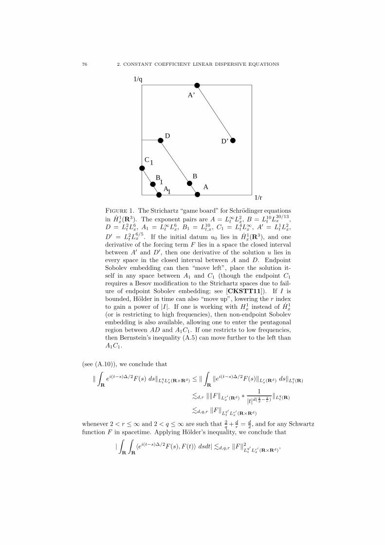
76 2. CONSTANT COEFFICIENT LINEAR DISPERSIVE EQUATIONS
1/r
1/q
A
A’
D
1
1
C
D’
B1
B
A
Figure 1. The Strichartz “game board” for Schrodinger equations
in H1x(R
3). The exponent pairs are A = L∞t L
2x, B = L10
t L30/13x ,
D = L2tL
6x, A1 = L∞
t L6x, B1 = L10
t,x, C1 = L4tL
∞x , A′ = L1
tL2x,
D′ = L2tL
6/5x . If the initial datum u0 lies in H1
x(R3), and one
derivative of the forcing term F lies in a space the closed intervalbetween A′ and D′, then one derivative of the solution u lies inevery space in the closed interval between A and D. EndpointSobolev embedding can then “move left”, place the solution it-self in any space between A1 and C1 (though the endpoint C1
requires a Besov modification to the Strichartz spaces due to fail-ure of endpoint Sobolev embedding; see [CKSTT11]). If I isbounded, Holder in time can also “move up”, lowering the r indexto gain a power of |I|. If one is working with H1
x instead of H1x
(or is restricting to high frequencies), then non-endpoint Sobolevembedding is also available, allowing one to enter the pentagonalregion between AD and A1C1. If one restricts to low frequencies,then Bernstein’s inequality (A.5) can move further to the left thanA1C1.
(see (A.10)), we conclude that
‖∫
R
ei(t−s)∆/2F (s) ds‖LqtL
rx(R×Rd) ≤ ‖
∫
R
‖ei(t−s)∆/2F (s)‖Lrx(Rd) ds‖Lq
t (R)
.d,r ‖‖F‖Lr′x (Rd) ∗
1
|t|d( 12− 1
r )‖Lq
t (R)
.d,q,r ‖F‖Lq′
t Lr′x (R×Rd)
whenever 2 < r ≤ ∞ and 2 < q ≤ ∞ are such that 2q + d
r = d2 , and for any Schwartz
function F in spacetime. Applying Holder’s inequality, we conclude that
|∫
R
∫
R
〈ei(t−s)∆/2F (s), F (t)〉 dsdt| .d,q,r ‖F‖2
Lq′
t Lr′x (R×Rd)
,

2.3. DISPERSION AND STRICHARTZ ESTIMATES 77
where 〈F,G〉 =∫Rd F (x)G(x) dx is the usual inner product. But the left-hand side
factorises as ‖∫Re−is∆/2F (s) ds‖2
L2x(Rd), and thus we obtain the dual homogeneous
Strichartz estimate
‖∫
R
e−is∆/2F (s) ds‖L2x(Rd) .d,q,r ‖F‖Lq′
t Lr′x (R×Rd)
which is (2.25). By duality we then obtain (2.24). Composing those two estimates,we conclude
‖∫
R
e−is∆/2F (s) ds‖LqtL
rx(Rd) .d,q,r,q,r ‖F‖Lq′
t Lr′x (R×Rd)
and (2.26) then follows from the Christ-Kiselev lemma.
Strichartz estimates can be viewed in two ways. Locally in time, they describea type of smoothing effect, but reflected in a gain of integrability rather thanregularity (if the datum is in L2
x, the solution u(t) is in Lrx with r > 2 for most ofthe time), and only if one averages in time. (For fixed time, no gain in integrabilityis possible; see Exercise 2.35.) Looking globally in time, they describe a decay effect,that the Lrx norm of a solution u(t) must decay to zero as t→ ∞, at least in someLqt -averaged sense. Both effects of the Strichartz estimate reflect the dispersivenature of the Schrodinger equation (i.e. that different frequencies propagate indifferent directions); it is easy to verify that no such estimates are available for thedispersionless transport equation (2.2), except with the trivial pair of exponents(q, r) = (∞, 2).
Remark 2.5. Readers who are familiar with the uncertainty principle (Prin-ciple A.1) can interpret the Strichartz estimates for the homogeneous Schrodingerequation as follows. Consider a solution u to the homogeneous Schrodinger equa-tion with L2
x norm O(1), and with frequency ∼ N (i.e. the Fourier transform issupported in the region |ξ| ∼ N), for each time t. The uncertainty principle showsthat at any given time t, the most that the solution u(t) can concentrate in physicalspace is in a ball of radius ∼ 1/N ; the L2
x normalisation then shows the solution canbe as large as Nd/2 on this ball. However, the Strichartz estimates show (roughlyspeaking) that such a strong concentration effect can only persist for a set of timesof measure ∼ 1/N2; outside of this set, the solution must disperse in physical space(compare with Proposition A.4). Note that this is also very consistent with Prin-ciple 2.1, since concentration in a ball of radius 1/N would induce the frequencyuncertainty of ∼ N , hence a velocity uncertainty of ∼ N , which should dispersethe ball after time ∼ 1/N2.
Similar Strichartz estimates can be established for any linear evolution equationwhich enjoys a dispersive estimate, such as the Airy equation. The wave equationalso obeys a dispersive inequality, see (2.19), (2.20), but the presence of the regular-izing factor φλ means that one requires some more harmonic analysis (in particular,some Littlewood-Paley theory and the theory of complex analytic interpolation) inorder to utilise this estimate properly. Nevertheless, it is still possible to establishsuitable Strichartz estimates for the wave equation. Indeed, we have
Theorem 2.6 (Strichartz estimates for wave equation). Let I be a time interval,and let u : I × Rd → C be a Schwartz solution to the wave equation u = F with

78 2. CONSTANT COEFFICIENT LINEAR DISPERSIVE EQUATIONS
1/r
1/q
A1A
A’1A’
EE’
F1
Figure 2. The Strichartz “game board” for wave equations inH1x(R
3). The exponent pairs are A = L∞t L
2x, E = L2
tL∞x , A1 =
L∞t L
6x, F1 = L4
tL12x , A′ = L1
tL2x, E
′ = L2tL
1x, A
′1 = L1
tL6/5x . If
the initial data (u0, u1) lies in H1x(R
3) × L2x(R
3), and a suitablederivative of the forcing term F on a space between A′ and E′
(excluding E′), then a certain derivative of u lies in every spacebetween A and E (excluding E), and so by Sobolev u itself lies inevery space between A1 and E (excluding E). At the endpoint A′,no derivatives on F are required. Also by Sobolev embedding, itwould have sufficed to place ∇F in any space between A′
1 and E(excluding E). Other moves, similar to those discussed in Figure1, are available.
c = 1, and with initial data u(t0) = u0, ∂tu(t0) = u1 for some t0 ∈ I. Then wehave the estimates
‖u‖LqtL
rx(I×Rd) + ‖u‖C0
t Hsx(I×Rd) + ‖∂tu‖C0
t Hs−1x (I×Rd)
.q,r,s,n
(‖u0‖Hs
x(Rd) + ‖u1‖Hs−1x (Rd) + ‖F‖
Lq′
t Lr′x (I×Rd)
)
whenever s ≥ 0, 2 ≤ q, q ≤ ∞ and 2 ≤ r, r <∞ obey the scaling condition
(2.27)1
q+d
r=d
2− s =
1
q′+d
r′− 2
and the wave admissibility conditions
1
q+d− 1
2r,1
q+d− 1
2r′≤ d− 1
4.
For a proof of this theorem, see [Kat8], [GV2], [Kap], [LSog], [Sog], [SStru3],[KTao]. Again, the exponents are sharp for the homogeneous version of theseestimates (i.e. with F = 0; see Exercise 2.43) but not the inhomogeneous; see [Har],[Obe], [Fos] for some inhomogeneous estimates not covered by the above theorem.The endpoint case r = ∞ contains a number of subtleties, see [FW] for some
2.3. DISPERSION AND STRICHARTZ ESTIMATES 79
discussion. As with the Schrodinger equation, the Strichartz estimates for the waveequation encode both local smoothing properties of the equation (the estimatesobtained from Strichartz lose fewer derivatives than the fixed-time estimates onewould get from Sobolev embedding), as well as global decay estimates, thoughwhen the wave equation compared against the Schrodinger equation in the samedimension, the estimates are somewhat inferior; this is due to the weaker dispersionin the wave equation (different frequencies move in different directions, but not indifferent speeds), the finite speed of propagation, and the concentration of solutionsalong light cones. This estimate only controls the homogeneous Sobolev norm, butthe lower order term in the inhomogeneous Sobolev norm can often be obtained byan integration in time argument.
An important special case of the wave equation Strichartz estimates is theenergy estimate
‖∇u‖C0tH
s−1x (I×Rd) + ‖∂tu‖C0
tHs−1x (I×Rd)
. ‖∇xu0‖Hs−1x (Rd) + ‖u1‖Hs−1
x (Rd) + ‖F‖L1tH
s−1x (I×Rd)
(2.28)
which can also be proven by other means, for instance via the Fourier transform(Exercise 2.45), or by using the stress energy tensor (see Exercise 2.59). Thisestimate has the useful feature of gaining a full degree of regularity; the forcingterm F is only assumed to have s− 1 degrees of regularity, but the final solution uhas s degrees of regularity. One also has the useful variant
‖u‖C0tH
sx(I×Rd) + ‖∂tu‖C0
tHs−1x (I×Rd)
.s 〈|I|〉(‖u0‖Hsx(Rd) + ‖u1‖Hs−1
x (Rd) + ‖F‖L1tH
s−1x (I×Rd)).
(2.29)
The other Strichartz estimates gain fewer than one full degree of regularity, butcompensates for this by improving the time and space integrability. One specificStrichartz estimate of interest (and one which was discovered in the original paper[Stri]) is the conformal Strichartz estimate for the wave equation
‖u‖L
2(d+1)/(d−1)t,x (R×Rd)
.d‖u(0)‖H
1/2x (Rd)
+ ‖∂tu(0)‖H
−1/2x (Rd)
+ ‖u‖L
2(d+1)/(d+3)t,x (R×Rd)
,(2.30)
valid for d ≥ 2.Strichartz estimates also exist for the Klein-Gordon equation but are more
difficult to state. See [MSW], [Nak4], [MN]; for short times one can just relyon the wave equation Strichartz estimates (treating the lower order mass term as aperturbation), while for long times it is easiest to proceed by treating the relativisticand non-relativistic regimes separately. Some Strichartz estimates are also knownin periodic settings, but primarily of L4
tL4x or L6
tL6x type, and are proven using the
spacetime Fourier transform, as one cannot exploit dispersion in these settings (asone can already see by considering plane wave solutions). See Section 2.6. Moregenerally, Strichartz estimates are closely related to restriction estimates for theFourier transform; see [Tao11] for a survey of the restriction phenomenon, whichhas been used to obtain a number of refinements (such as bilinear refinements) tothe Strichartz inequalities.
Exercise 2.34 (Asymptotic Lpx behaviour of Schrodinger). Let u0 ∈ Sx(Rd)be a non-zero Schwartz function whose Fourier transform u0(ξ) is supported in theball |ξ| ≤ 1. Show that we have the estimate |eit∆u0(x)| .N,u0 〈t〉−N 〈x〉−N for all

80 2. CONSTANT COEFFICIENT LINEAR DISPERSIVE EQUATIONS
times t, all N > 0, and all x such that |x| ≥ 5|t|. (Hint: use rotational symmetry tomake x a multiple of the unit vector e1, thus x = (x1, 0, . . . , 0). Then use the Fourierrepresentation (2.12) of eit∆u0(x), followed by repeated integration by parts in thex1 direction.) In the region |x| < 5|t|, obtain the estimate |eit∆u0(x)| .u0 〈t〉−d/2.Conclude that ‖eit∆u0‖Lp
x(Rd) ∼d,u0,p 〈t〉d( 1p− 1
2 ) for all 1 ≤ p ≤ ∞. (Hint: firstestablish this for p = 2, obtain the upper bound for all p, and then use Holder’sinequality to obtain the lower bound.)
Exercise 2.35 (Necessary conditions for fixed-time Schrodinger). Suppose 1 ≤p, q ≤ ∞ and α ∈ R are such that the fixed-time estimate
‖eit∆/2u0‖Lqx(Rd) ≤ Ctα‖u0‖Lp
x(Rd)
for all u0 ∈ Sx(Rd) and t 6= 0, and some C independent of t and u0. Usingscaling arguments, conclude that α = d
2 (1q − 1
p ). Using (2.34) (and time translation
invariance), conclude that q ≥ p and q = p′ (and thus 1 ≤ p ≤ 2). In particular theSchrodinger operators are not bounded on any Lpx(R
d) space except when p = 2.Indeed, a good rule of thumb is that dispersive evolution operators only preserve“L2
x-based” spaces and no others (with the notable exception of the one-dimensionalwave evolution operators, which are not truly dispersive).
Exercise 2.36 (Schrodinger Strichartz cannot gain regularity). Using Galileaninvariance (Exercise 2.5), show that no estimate of the form
‖ei∆/2u0‖W s2,qx (Rd) ≤ C‖u0‖W s1,p
x (Rd)
or
‖eit∆/2u0‖LqtW
s2,rx ([0,1]×Rd) ≤ C‖u0‖W s1,p
x (Rd)
can hold with C independent of u0, unless s2 ≤ s1.
Exercise 2.37 (Decay of finite energy Schrodinger solutions). Show that theadmissible space L∞
t L2x which appears in Theorem 2.3 can be replaced by the
slightly smaller space C0t L
2x. Similarly, if u0 ∈ H1
x(R3) and u : R × R3 → C
is the solution to the Schrodinger equation, show that limt→±∞ ‖u(t)‖Lpx(R3) for
2 < p ≤ 6 and that
limt→±∞
‖〈x〉−εu(t)‖L2x
+ ‖〈x〉−ε∇u(t)‖L2x
= 0
for any ε > 0 (see [Tao8] for an application of these estimates to nonlinearSchrodinger equations).
Exercise 2.38 (Pseudoconformal invariance of Strichartz). (Pieter Blue, pri-vate communication) Show that if q, r are Schrodinger-admissible exponents, thenthe space LqtL
rx(R × Rd) is preserved under the pseudoconformal transformation
(Exercise 2.28). Conclude that Theorem 2.3 is invariant under the pseudocon-formal transformation. (It is also invariant under space and time translations,homogeneity, scaling, phase rotation, time reflection, spatial rotation and Galileantransformations.)
Exercise 2.39 (Conformal invariance of Strichartz). Show that the conformalStrichartz estimate (2.30) is invariant under space and time translations, homogene-ity, scaling, phase rotation, time reflection, spatial rotation, Lorentz transformation(Exercise 2.6), and conformal inversion (Exercise 2.14).

2.3. DISPERSION AND STRICHARTZ ESTIMATES 81
Exercise 2.40. Show that Lemma 2.4 fails at the endpoint p = q, even whenX and Y are scalar. (Hint: take p = q = 2 and consider truncated versions of the
Hilbert transform Hf(t) = p.v.∫ f(s)t−s ds.)
Exercise 2.41. Using Exercise 2.30, establish some Strichartz estimates forthe Airy equation. (As it turns out, when it comes to controlling equations ofKorteweg-de Vries type, these estimates are not as strong as some other estimatesfor the Airy equation such as local smoothing and Xs,b estimates, which we shalldiscuss later in this chapter.)
Exercise 2.42. Using the scale invariance from Exercise 2.9, show that thecondition 2
q + dr = d
2 is necessary in order for (2.24). Next, by superimposing
multiple time-translated copies of a single solution together (thus replacing u(t, x)
by∑Nj=1 u(t − tj , x) for some widely separated times t1, . . . , tN ) show that the
condition q ≥ 2 is also necessary. (The double endpoint (q, r, d) = (2,∞, 2) isharder to rule out, and requires a counterexample constructed using Brownianmotion; see [Mon].) Note that similar arguments will establish the necessity of(2.27), as well as the requirements q, q ≥ 2 in Theorem 2.6.
Exercise 2.43 (Knapp example). Consider the solution u : R1+d → C to thewave equation with c = 1 given by
u(t, x) :=
∫
1≤ξ1≤2;|ξ2|,...,|ξn|≤εeix·ξeit|ξ| dξ
where 0 < ε < 1 is a small number. Show that u(t, x) is comparable in magnitudeto εd−1 whenever |t| ≪ 1/ε2, |x1 + t| ≪ 1 and |x2|, . . . , |xn| ≪ 1/ε. Use this toconclude that the condition 1
q + d−12r ≤ d−1
4 in Theorem 2.6 cannot be improved.
One can also obtain essentially the same example by starting with a bump functioninitial datum, and applying a Lorentz transform (see Exercise 2.6) with velocityv := (1− ε2)e1; the strange rectangular region of spacetime obtained above is thenexplainable using the familiar phenomena of time dilation and length contractionin special relativity.
Exercise 2.44 (Stein example). Let 1/2 < α ≤ 1, and let g ∈ L2x(R
3) be thefunction
g(x) :=1B(2e3,2)\B(e3,1)(x)
|x|2〈log |x|〉α ,
where e3 is the third unit vector of R3 and B(x, r) denotes the ball of radius r
centred at x. Show that ‖g‖L2x(R3) = Oα(1), but that the solution u(t) := sin(t
√−∆√
−∆g
to the homogeneous wave equation with initial position 0 and initial velocity g obeysu(te3, t) = ∞ for all 1 ≤ t ≤ 2. (Hint: use Exercise 2.31.) In particular, Theorem2.6 fails at the endpoint (q, r) = (2,∞), a fact first observed (with a more indirectproof) in [KM].
Exercise 2.45. Prove the energy estimate (2.28) using (2.14), the Fouriertransform, and Minkowski’s inequality. Note that the implied constant in the .notation is absolute (not depending on s or d). Then deduce (2.29).
Exercise 2.46 (Besov version of Strichartz estimates). For each dyadic num-ber N , let PN be the Littlewood-Paley multiplier at frequency N , as defined in
82 2. CONSTANT COEFFICIENT LINEAR DISPERSIVE EQUATIONS
Appendix A. By means of complex interpolation, establish the inequalities
‖u‖LqtL
rx(I×Rd) .q,r (
∑
N
‖PNu‖2Lq
tLrx(I×Rd))
1/2
whenever 2 ≤ q, r ≤ ∞ (so in particular whenever q, r are admissible exponents forStrichartz estimates), as well as the “dual” estimate
(∑
N
‖PNF‖2
Lq′
t Lr′x (I×Rd)
)1/2 .q,r ‖F‖Lq′
t Lr′x (I×Rd)
for the same range of q, r. (Note that to apply interpolation properly for the firstinequality, you will need to write u as an appropriate linear operator applied tothe functions uN = PNu.) By exploiting the fact that PN commutes with theSchrodinger operator i∂t + ∆, establish the estimate
(∑
N
‖PNeit∆/2u0‖2Lq
tLrx(R×Rd))
1/2 .d,q,r ‖u0‖L2x(Rd)
for all Schrodinger-admissible q, r. Similarly establish analogues of (2.25) and(2.26).
2.4. Conservation laws for the Schrodinger equation
Knowledge about life is one thing; effective occupation of a placein life, with its dynamic currents passing through your being, isanother. (William James, “The Varieties of Religious Experience”)
In Hamiltonian ODE, one often encounters conserved quantities E(t) of the flowsuch as energy, momentum, mass, and so forth. One has similar conserved quan-tities in Hamiltonian PDE, but they come with additional structure. Namely, thetypical conserved quantity E(t) that one encounters is not just a scalar quantity, butis also an integral of some density e0(t, x), thus for instance E(t) =
∫Rd e0(t, x) dx.
The conservation of E(t) can then be manifested in a more local form by the point-wise conservation law15
(2.31) ∂te0(t, x) + ∂xjej(t, x) = 0
for some vector-valued16 quantity ej , which is thus the current associated to thedensity e0. The conservation of E then follows (formally, at least) by integratingthe continuity equation in space and using the divergence theorem (assuming somesuitable spatial decay on the current, of course). Thus in PDE, conservation lawscome in both integral and differential forms. The differential form of the conserva-tion law is significantly more flexible and powerful than the integral formulation, asit can be localised to any given region of spacetime by integrating against a suitablecutoff function (or contracting against a suitable vector field). Of course, when onedoes so, one may no longer get a perfectly conserved quantity, but one often obtainsa quantity which is almost conserved (the derivative in time is small or somehow“lower order”) or perhaps monotone. Thus from a single conservation law one cangenerate a variety of useful estimates, which can serve to constrain the direction of
15Roman indices such as j and k will be summed over the spatial indices 1, . . . , d in the usualmanner; Greek indices such as α and β will be summed over 0, . . . , d.
16In some cases E and e0 are themselves vector-valued instead of scalar, in which case ej
will be tensor-valued.

2.4. CONSERVATION LAWS FOR THE SCHRODINGER EQUATION 83
propagation of a solution, or at least of various components of that solution (e.g.the high frequency components).
These conservation laws are particularly useful for controlling the long-timedispersive behaviour, or short-time smoothing behaviour, of nonlinear PDE, butto illustrate the concepts let us just work first with the linear analogues of thesePDE. To make the discussion concrete, we focus on the Schrodinger equation (2.3)with ~ = m = 1, thus
(2.32) i∂tu+1
2∆u = 0;
to avoid technicalities we consider only smooth solutions u ∈ C∞t,locSx(R×Rd). In
practice one can usually extend the estimates here to rougher solutions by limitingarguments or duality.
Before we discuss the differential form of the conservation laws, let us firstrecall the integral form of the conservation laws and their connection (via Noether’stheorem) to various symmetries (cf. Table 1 from Chapter 1); we will justify theirconservation later when considering the differential form of these laws, and alsomore informally in Exercise 2.47 below. The symmetry of phase rotation, u(t, x) 7→eiθu(t, x), leads to the scalar conserved quantity
M(t) :=
∫
Rd
|u(t, x)|2 dx,
which is variously referred to as the total probability, charge, or mass in the lit-erature. The symmetry of space translation, u(t, x) 7→ u(t, x − x0), leads to thevector-valued conserved quantity ~p(t), defined in coordinates as
pj(t) :=
∫
Rd
Im(u(t, x)∂xju(t, x)) dx,
which is the total momentum. The symmetry of time translation, u(t, x) 7→ u(t −t0, x), leads to the conserved quantity
E(t) :=1
2
∫
Rd
|∇u(t, x)|2 dx,
known as the total energy or Hamiltonian. The symmetry of Galilean invariance(Exercise 2.5) leads to the conserved quantity
∫
Rd
x|u(t, x)|2 dx− t~p(t),
which is the normalised centre-of-mass. The pseudo-conformal symmetry (Exercise2.28) does not directly lead to a conserved quantity, as it is a discrete symmetryrather than a continuous one. However, it can be used to conjugate some of the pre-ceding symmetries and generate new ones. The pseudo-conformal symmetry leavesthe mass invariant, as that symmetry commutes with phase rotation; it also swapsmomentum conservation with the conservation of normalised centre-of-mass, as thepseudo-conformal symmetry intertwines spatial transation and Galilean invariance.The energy conjugates to the pseudo-conformal energy
(2.33)1
2‖(x+ it∇)u(t)‖2
L2x(Rd)

84 2. CONSTANT COEFFICIENT LINEAR DISPERSIVE EQUATIONS
which is also conserved. In particular, we see from the triangle inequality andconservation of energy that
(2.34) ‖|x|u(t)‖L2x(Rd) ≤ ‖|x|u(0)‖L2
x(Rd) + t‖∇u(0)‖L2x(Rd),
which is an estimate establishing a kind of approximate finite speed of propagationresult for finite energy solutions. See also Exercise 2.49.
Now we analyze the local versions of these conserved quantities. It is convenientto introduce the pseudo-stress-energy tensor Tαβ , defined for α, β = 0, 1, . . . , n andon the spacetime R × Rd by
T00 = |u|2
T0j = Tj0 = Im(u∂xju)
Tjk = Re(∂xju∂xku) − 1
4δjk∆(|u|2)
for all j, k = 1, . . . , d, where δjk is the Kronecker delta (thus it equals 1 when j = kand zero otherwise). A direct computation using (2.32) then verifies (for smoothfields u, at least) the local conservation laws
(2.35) ∂tT00 + ∂xj T0j = 0; ∂tTj0 + ∂xkTjk = 0.
The quantity T00 is known as the mass density, the quantity T0j = Tj0 is knownas both the mass current and the momentum density, and the quantity Tjk is themomentum current or stress tensor. For smooth, rapidly decreasing solutions u,this verifies the conservation of mass and momentum asserted earlier, since
M(t) =
∫
Rd
T00(t, x) dx; pj(t) = −∫
Rd
T0j(t, x) dx.
Conservation of energy also has a local formulation, though not one related to thepseudo-stress-energy tensor17 Tαβ (Exercise 2.48).
By multiplying first equation in (2.35) by a smooth function a(x) of at mostpolynomial growth, integrating in space, and then integrating by parts, we obtainthe identity
(2.36) ∂t
∫
Rd
a(x)|u(t, x)|2 dx =
∫
Rd
∂xja(x)Im(u(t, x)∂xju(t, x)) dx.
This identity can be used to control the local rate of change of mass by quantitiessuch as the energy (see Exercises 2.50, 2.51).
17See however Exercise 3.30.
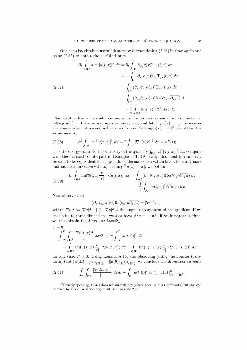
2.4. CONSERVATION LAWS FOR THE SCHRODINGER EQUATION 85
One can also obtain a useful identity by differentiating (2.36) in time again andusing (2.35) to obtain the useful identity
∂2t
∫
Rd
a(x)|u(t, x)|2 dx = ∂t
∫
Rd
∂xja(x)T0j(t, x) dx
= −∫
Rd
∂xja(x)∂xkTjk(t, x) dx
=
∫
Rd
(∂xj∂xka(x))Tjk(t, x) dx
=
∫
Rd
(∂xj∂xka(x))Re(∂xju∂xk
u) dx
− 1
4
∫
Rd
|u(t, x)|2∆2a(x) dx.
(2.37)
This identity has some useful consequences for various values of a. For instance,letting a(x) = 1 we recover mass conservation, and letting a(x) = xj we recoverthe conservation of normalised centre of mass. Setting a(x) = |x|2, we obtain thevirial identity
(2.38) ∂2t
∫
Rd
|x|2|u(t, x)|2 dx = 2
∫
Rd
|∇u(t, x)|2 dx = 4E(t);
thus the energy controls the convexity of the quantity∫Rd |x|2|u(t, x)|2 dx; compare
with the classical counterpart in Example 1.31. (Actually, this identity can easilybe seen to be equivalent to the pseudo-conformal conservation law after using massand momentum conservation.) Setting18 a(x) = |x|, we obtain
∂t
∫
Rd
Im(u(t, x)x
|x| · ∇u(t, x)) dx =
∫
Rd
(∂xj∂xka(x))Re(∂xju∂xk
u) dx
− 1
4
∫
Rd
|u(t, x)|2∆2a(x) dx.
(2.39)
Now observe that
(∂xj∂xka(x))Re(∂xju∂xk
u) = |∇/ u|2/|x|,where |∇/ u|2 := |∇u|2 − | x|x| · ∇u|2 is the angular component of the gradient. If we
specialise to three dimensions, we also have ∆2a = −4πδ. If we integrate in time,we thus obtain the Morawetz identity
∫ T
−T
∫
R3
|∇/ u(t, x)|2|x| dxdt + 4π
∫ T
−T|u(t, 0)|2 dt
=
∫
R3
Im(u(T, x)x
|x| · ∇u(T, x)) dx−∫
R3
Im(u(−T, x) x|x| · ∇u(−T, x)) dx
(2.40)
for any time T > 0. Using Lemma A.10, and observing (using the Fourier trans-form) that ‖u(±T )‖
H1/2x (R3)
= ‖u(0)‖H
1/2x (R3)
, we conclude the Morawetz estimate
(2.41)
∫
R
∫
R3
|∇/ u(t, x)|2|x| dxdt+
∫
R
|u(t, 0)|2 dt . ‖u(0)‖2
H1/2x (R3)
.
18Strictly speaking, (2.37) does not directly apply here because a is not smooth, but this canbe fixed by a regularisation argument; see Exercise 2.57.

86 2. CONSTANT COEFFICIENT LINEAR DISPERSIVE EQUATIONS
This estimate can be thought of as a variant of a Strichartz estimate, obtainingsome smoothing and decay near the spatial origin x = 0; it should be comparedwith Example 1.32. It has a significant advantage over the Strichartz estimate, inthat it extends with only minor modification to the case of defocusing nonlinearSchrodinger equations; see Section 3.5, in which we also discuss an interactionversion of the above estimate. One can also extend this three-dimensional estimateto higher dimensions. For lower dimensions there are some additional subtleties;see [Nak2].
Exercise 2.47. Let us formally consider L2x(R
d → C) as a symplectic phase
space with symplectic form ω(u, v) = −2∫Rd Im(u(x)v(x)) dx. Show that the
Schrodinger equation (2.3) with ~ = m = 1 is then the formal Hamiltonian flowassociated to the (densely defined) Hamiltonian H(u) := 1
2
∫Rd |∇u|2 dx. Also use
this flow to formally connect the symmetries and conserved quantities mentionedin this section via Noether’s theorem (ignoring irrelevant constants such as factorsof 2). See [Kuk3] for a more rigorous treatment of this infinite-dimensional Hamil-tonian perspective, and [SSul] for a Lagrangian perspective of the material in thissection.
Exercise 2.48. Obtain a local conservation law (2.31) for the energy densitye0 = 1
2 |∇u|2 for the Schrodinger equation.
Exercise 2.49 (Local smoothing from localised data). Let u ∈ C∞t,locSx(R ×
Rd) be a smooth solution to the Schrodinger equation (2.32) with ~ = m = 1. Byusing mass conservation and the pseudo-conformal conservation law, establish thebound
‖∇u(t)‖L2x(BR) .d
〈R〉|t| ‖〈x〉u(0)‖L2
x(Rd)
for all t 6= 0 and R > 0, where BR := x ∈ Rd : |x| ≤ R is the spatial ball of radiusR. This shows that localisation of initial data leads to a local gain of regularity(by a full derivative, in this case) at later times, together with some local decay intime.
Exercise 2.50 (Local near-conservation of mass). Let u ∈ C∞t,locSx(R × Rd)
be a smooth solution to the Schrodinger equation (2.32) with ~ = m = 1, and withenergy E = 1
2‖∇u(0)‖2L2
x(Rd). Show that for any R > 0 and t 6= 0 we have
(
∫
|x|≤R|u(t, x)|2 dx)1/2 ≤ (
∫
|x|≤2R
|u(0, x)|2 dx)1/2 +Od(E1/2|t|R
).
(Hint: apply (2.36) with a(x) = φ2(x/R), where φ is a bump function supported onthe ball of radius 2 which equals 1 on the ball of radius 1, and obtain a differentialinequality for the quantity M(t) := (
∫Rd φ
2(x/R)|u(t, x)|2 dx)1/2.) This estimate(and the generalisation in Exercise 2.51 below) is especially useful for the energy-
critical nonlinear Schrodinger equation, as the error term of CE1/2|t|R depends only
on the energy of u and not on other quantities such as the mass; see [Gri5], [Bou7],[Bou9], [Tao9] for some applications of this estimate.
Exercise 2.51 (Local near-conservation of mass, II). [Bou7], [Bou9] Let thenotation and assumptions be as in Exercise 2.50. Prove the more general inequality
(
∫
|x|≤R|u(t, x)|2 dx)1/2 ≤ (
∫
|x|≤2nR
|u(0, x)|2 dx)1/2 +Od(E1/2|t|Rn1/2
)

2.4. CONSERVATION LAWS FOR THE SCHRODINGER EQUATION 87
for any integer n ≥ 1; this improves the error term at the cost of enlarging the ballin the main term. (Hint: We may use time reversal symmetry to take t > 0. Useconservation of energy and the pigeonhole principle to locate an integer 1 ≤ j ≤ n
such that∫ t0
∫2jR≤|x|≤2j+1R |∇u(t, x)|2 dxdt . Et/n. Then apply the argument used
to establish Exercise 2.50, but with R replaced by 2jR.) This example shows thatone can sometimes exploit the pigeonhole principle to ameliorate “boundary effects”caused by cutoff functions; for another instance of this idea, see [CKSTT11]. Inthis particular case it turns out that one can use Exercise 2.50 (with R replaced by2n−1R) to replace the n1/2 denominator by the much stronger 2n term, howeverthere are other situations in which the pigeonhole principle is the only way to obtaina satisfactory estimate.
Exercise 2.52 (Weighted Sobolev spaces). For any integer k ≥ 0, define theweighted Sobolev space Hk,k
x (Rd) be the closure of the Schwartz functions underthe norm
‖u‖Hk,kx (Rd) :=
k∑
j=0
‖〈x〉ju‖Hk−jx (Rd).
Establish the estimate
‖eit∆/2f‖Hk,kx (Rd) .k,d 〈t〉k‖f‖Hk,k
x (Rd)
for all Schwartz f , either using the Fourier transform or by using mass conser-vation laws (and higher order variants of these laws, exploiting the fact that theSchrodinger equation commutes with derivatives). (Hint: if you are really stuck,try working out the k = 1 case first.)
Exercise 2.53 (Local smoothing for Schrodinger). [Sjo],[Veg],[CS] Let u ∈C∞t,locSx(R × R3) be a smooth solution to the Schrodinger equation (2.32) with
~ = m = 1. Establish the homogeneous local smoothing estimate
∫
R
∫
R3
〈x〉−1−ε|∇u(t, x)|2 + 〈x〉−3−ε|u(t, x)|2 dxdt .ε ‖u(0, x)‖2
H1/2x (R3)
for all ε > 0. (Hint: One can take ε to be small. Then adapt the Morawetzargument in the text with a(x) := 〈x〉 − ε〈x〉1−ε.) This shows a local gain of half aderivative for the homogeneous Schrodinger equation. Give an informal explanationas to why this estimate is consistent with the Heisenberg law v = ξ that arises fromPrinciple 2.1; compare it also with Example 1.33.
Exercise 2.54 (Local smoothing for Schrodinger, II). Let u ∈ C∞t,locSx(R×R3)
be a smooth solution to the inhomogeneous Schrodinger equation
i∂tu+ ∆u = F.
Establish the dual local smoothing estimate
supt∈R
‖u(t)‖H
1/2x (R3)
.ε ‖u(0)‖H
1/2x (R3)
+
∫
R
∫
R3
〈x〉1+ε|F (t, x)|2 dxdt

88 2. CONSTANT COEFFICIENT LINEAR DISPERSIVE EQUATIONS
for any ε > 0. (Hint: use Exercise 2.53 and Duhamel’s formula.) Then establishthe retarded local smoothing estimate
∫
R
∫
R3
〈x〉−1−ε|∇u(t, x)|2 + 〈x〉−3−ε|u(t, x)|2 dxdt
.ε ‖u(0, x)‖2
H1/2x (R3)
+
∫
R
∫
R3
〈x〉1+ε|F (t, x)|2 dxdt.
(Hint: use the same argument19 as in Exercise 2.53. An additional interaction termbetween u and F will appear, and can be controlled using Cauchy-Schwarz.) Thisshows a local gain of a full derivative for the in homogeneous Schrodinger equation.
Exercise 2.55 (Local smoothing for Airy equation). [Kat2], [KF] Show thatsmooth solutions u ∈ C∞
t,locSx(R × R → R) to the Airy equation ∂tu + ∂3xu = 0
obey the conservation law
(2.42) ∂t(u2) = −∂3
x(u2) + 3∂x(u
2x)
where ux := ∂xu, and use this to conclude the local smoothing estimate
(2.43)
∫ T
0
∫
|x|≤Ru2x dxdt .
T +R3
R2
∫
R
u(0, x)2 dx
for all T > 0 and R > 0. (Hint: first integrate (2.42) against the constant function1 to establish L2
x conservation, and then integrate instead against a suitable cutofffunction which equals 1 for x > 2R, zero for x < −2R, and increases steadily for−R < x < R.)
Exercise 2.56 (Sharp local smoothing for Airy equation). [KPV2] With thenotation as in the preceding exercise, prove the sharper estimate
∫
R
ux(t, x0)2 dt .
∫
R
u(0, x)2 dx
for any x0 ∈ R, so that the factor T+R3
R2 in (2.43) can be replaced with R. (Hint: usetranslation invariance to set x0 = 0, and use the Fourier representation of ux(t, 0),followed by Plancherel’s theorem. Unlike (2.43), it seems difficult to establish thisestimate purely using conservation law techniques, thus suggesting some limitationsto that method.) Give an informal explanation as to why (2.43) is consistentwith the dispersion relation v = −3ξ2 that arises from Principle 2.1. What is theanalogous estimate for the one-dimensional Schrodinger equation?
Exercise 2.57. Justify the derivation of (2.39) from (2.37) (for C∞t,locSx solu-
tions u to the Schrodinger equation) by applying (2.37) with a(x) :=√ε2 + |x|2
and then taking limits as ε→ 0. These types of regularisation arguments are quitecommon in the theory of linear and nonlinear PDE, and allow one to extend thevalidity of many formal computations well beyond the regularities that would beneeded to justify them classically.
19We thank Jared Wunsch for pointing out this simple argument.

2.5. THE WAVE EQUATION STRESS-ENERGY TENSOR 89
2.5. The wave equation stress-energy tensor
A man must drive his energy, not be driven by it. (William Fred-erick Book)
Having considered conservation laws for the Schrodinger equation, we turn tothe wave equation
(2.44) ∂α∂αu = F,
where we take smooth scalar fields u ∈ C∞t,locSx(R1+d → C) for simplicity. In
particular u has sufficient regularity and decay at infinity to justify all integrationby parts computations.
While it is possible to view the wave equation as a Hamiltonian system (seeExercise 2.58), the geometry of Minkowski space suggests that one can also alter-nately view the wave equation (and the associated conservation laws) in a moreLorentz-invariant way; thus our perspective here will be slightly different fromthat in the preceding section. Indeed, one can view the wave equation in a La-grangian manner instead, viewing u as a formal critical point of the Lagrangianfunctional 1
2
∫R1+d ∂
αu∂αu dg. This functional is formally invariant under diffeo-morphic changes of variable; by considering the variation of the functional alongan infinitesimal such change of variable (see Exercise 2.60) one can then construct
a stress-energy tensor Tαβ for this equation, which in this case is
(2.45) Tαβ := Re(∂αu∂βu) − 1
2gαβRe(∂γu∂γu).
In coordinates with the normalisation c = 1, we have
T00 = T00 =1
2|∂tu|2 +
1
2|∇u|2
T0j = −T0j = −Re(∂tu∂xju)
Tjk = Tjk = Re(∂xju∂xku) − δjk
2(|∇u|2 − |∂tu|2).
This tensor is real and symmetric. The quantity T00 is known as the energy den-sity, the quantity T0j is the energy current or momentum density, and Tjk is themomentum current or stress tensor. The similarity with the Schrodinger pseudo-stress-energy tensor is not accidental; see Exercise 3.30.
The tensor Tαβ is clearly symmetric, and a quick computation using (2.44)yields the divergence equation
(2.46) ∂αTαβ = Re((∂βu)F ).
Henceforth we consider the homogeneous equation F ≡ 0, so that T is divergencefree. In coordinates, we thus have
∂tT00 + ∂xjT
0j = 0; ∂tT0j + ∂xk
Tjk = 0
(compare with (2.35)). This already yields conservation of the total energy
E[u(t)] = E(t) :=
∫
Rd
T00(t, x) dx
and the total momentum
pj(t) :=
∫
Rd
T0j(t, x) dx,
90 2. CONSTANT COEFFICIENT LINEAR DISPERSIVE EQUATIONS
assuming sufficient spatial decay of course on the solution u and its derivatives.It turns out that these conservation laws can be nicely localised in spacetime
by exploiting the positivity property
(2.47) Tαβvαvβ ≥ 0
whenever vα is a time-like or light-like vector (so vαvα ≤ 0). Indeed from (2.45) wehave
Tαβvαvβ = (vα∂αu)2 − 1
2(vαvα)(∂γu)(∂γu)
which is clearly non-negative in the light-like case vαvα = 0, and in the timelikecase one can check positivity by dividing the gradient ∂αu into the componentparallel to v and the component Minkowski-orthogonal to v (on which the metricg is spacelike, hence non-negative); alternatively one can use Lorentz invariance to
reduce to the case20 v = ∂t. More generally we have Tαβvαwβ ≥ 0 whenever v, ware time-like or light-like, and both future-oriented (see Exercise 3.41). To exploitthis positivity, we can use Stokes’ theorem to obtain the identity
(2.48)
∫
Σ1
TαβXαnβdS =
∫
Σ0
TαβXαnβdS +
∫
Σ
∂β(TαβXα)dg
for an arbitrary smooth vector field Xα, where Σ is an open region in spacetimebounded below by a spacelike hypersurface Σ0 and above by a spacelike hypersur-face Σ1, nβ is the positive timelike unit normal and dS is the induced measure fromthe metric g (which is positive on the spacelike surfaces Σ0, Σ1); if Σ is unboundedthen of course we need to assume suitable decay hypotheses on u or X . For in-stance, if Σ0 = (t, x) : t = 0, Σ1 = (t, x) : t = t1 and X = ∂t for some arbitrarytime t1 ∈ R we obtain the conservation of energy E(t1) = E(0), while if we insteadtake X = ∂xj we obtain conservation of momentum pj(t1) = pj(0). Now supposethat T∗ > t1 > 0, and we take Σ0 to be the disk (t, x) : t = 0, |x| ≤ T∗ and Σ1 tobe the truncated cone21
Σ1 := (t, x) : 0 < t < t1, |x| = T∗ − t ∪ (t, x) : t = t1, |x| ≤ T∗ − t1.Setting X = ∂t, we conclude the energy flux identity
(2.49)
∫
|x|≤T∗−t1T00(t1, x) dx+ FluxT∗ [0, t1] =
∫
|x|≤T∗
T00(0, x) dx
where FluxT∗ [t0, t1] is defined for 0 ≤ t0 < t1 < T∗ by
FluxT∗ [t0, t1] :=
∫
t0<t<t1,|x|=T∗−tTαβXαnβdS.
Intuitively, this identity asserts that the energy at the top of the truncated cone,plus the energy flux escaping the sides of the cone, is equal to the original energyat the base of the cone. From (2.47) we see that FluxT∗ [0, t1] is non-negative, andso we have the localised energy monotonicity formula∫
|x|≤T∗−t1T00(t1, x) dx ≤
∫
|x|≤T∗
T00(0, x) dx
20We of course equate a vector field Xα with the associated first-order differential operatorXα∂α in the usual manner.
21Strictly speaking, Σ1 is not quite spacelike, which causes dS to degenerate to zero and nβ
to elongate to infinity. But the area form nβdS remains well defined in the limit; we omit the
standard details.
2.5. THE WAVE EQUATION STRESS-ENERGY TENSOR 91
In particular, we have obtained the finite speed of propagation property: if u solvesthe wave equation, and vanishes on the ball |x| ≤ T∗ at time t = 0, then it vanisheson the smaller ball |x| ≤ T∗−t1 for all times 0 < t1 < T∗; this reflects the well-knownfact that solutions to wave equations cannot propagate faster than the speed of light(which has been normalised to c = 1 here). Also, from the energy flux identity andenergy conservation we have
(2.50) FluxT∗ [0, t1] ≤ E(0);
thus if the solution has finite energy, then FluxT∗ [0, t1] is monotone increasing int1 and is also bounded. It therefore converges22 to some limit as t1 → T∗; sinceFluxT∗ [t0, t1] = FluxT∗ [0, t1]−FluxT∗ [0, t0], we conclude in particular the flux decayproperty
limt0,t1→T∗
FluxT∗ [t0, t1] = 0.
This shows that near the tip (T∗, 0) of the cone, an asymptotically vanishing amountof energy will escape the sides of the cone. There is however still the possibility ofenergy concentration, in which the energy stays inside the cone and concentrates tothe tip as t→ T∗; we shall discuss this possibility further in Section 5.1.
To exploit (2.48) and (2.47) further, it is of interest to understand the diver-
gence23 of vector fields of the form TαβXβ. Indeed we see from (2.46) and the
symmetry of T that the vector field TαβXβ has divergence
(2.51) ∂α(TαβXβ) =1
2Tαβπαβ
where παβ is the deformation tensor
(2.52) παβ := ∂αXβ + ∂βXα = LXgαβ ,where LX denotes the Lie derivative. In particular, if the vector field X is aKilling vector field (i.e. the diffeomorphism induced by X preserves the metric),
then LXgαβ = 0 and hence TαβXβ is divergence-free. In particular, we obtainconservation of the quantity
∫
Rd
T0βXβ(t, x) dx
For instance, the vector fields ∂t and ∂xj , which correspond to time translation andspatial translation respectively, yield the conservation of energy and momentumrespectively. If instead we take the rotation vector field xj∂xk
− xk∂xj for somefixed 1 ≤ j < k ≤ n, which is clearly Killing, we obtain the conservation of angularmomentum∫
Rd
xjT0k(t, x) − xkT
0j(t, x) dx = Re
∫
Rd
∂tu(t, x)(xk∂xj − xj∂xk)u(t, x) dx.
22This innocuous statement from basic real analysis - that every monotone bounded sequenceconverges - is surprisingly useful in the analysis of PDE, as it allows one to convert a monotonicityformula (say for a sequence an) into a decay estimate (for the Cauchy differences an − am). Thedrawback is that the decay is qualitative only; there is no uniform control on the decay of thean − am, although one can see that these differences cannot be too large for too many disjointintervals [n, m].
23We thank Markus Keel and Sergiu Klainerman for sharing some unpublished notes on thistopic, which were very helpful in preparing the material in this section.

92 2. CONSTANT COEFFICIENT LINEAR DISPERSIVE EQUATIONS
Taking instead the Lorentz vector field xj∂t + t∂xj , which is also Killing, we obtainconservation of normalised centre-of-mass∫
Rd
xjT00(t, x) − tT0j(t, x) dx =
∫
Rd
xjT00(t, x) dx− tpj .
Thus Lorentz invariance plays the role in the wave equation that Galilean invariancedoes for the Schrodinger equation.
Unfortunately, there are no further Killing vector fields for Minkowski space(other than taking linear combinations of the ones listed above); this is the hyper-bolic analogue of the well-known fact that the only orientation-preserving isometriesof Euclidean space (i.e. the rigid motions) are the translations and rotations, andcombinations thereof; see Exercise 2.62. However, there is a slightly larger class ofconformal Killing vector fields, where the deformation tensor παβ does not vanish,but is instead a scalar multiple of gαβ , thus παβ = Ωgαβ for some scalar functionΩ. Inserting this and (2.45) into (2.51), and observing that gαβg
αβ = (d + 1), weconclude that for a conformal Killing field we have
∂α(TαβXβ) = −d− 1
4ΩRe(∂γu∂γu).
Using the equation (2.44), we can rewrite this further as
∂α(TαβXβ) = −d− 1
8Ω∂γ∂γ(|u|2),
which rearranges as
(2.53) ∂αPα = −d− 1
8|u|2Ω
where Pα is the vector field
Pα := TαβXβ +d− 1
8(Ω∂α(|u|2) − (∂αΩ)|u|2).
This is quite close to being a conservation law; note that Pα contains terms whichare quadratic in the first derivatives of u, but the divergence of Pα only containsterms of zeroth order in u.
To give some examples of (2.53), let us first consider the Morawetz vector fieldX associated to (t2+|x|2)∂t+2txj∂xj (i.e. X0 = −(t2+|x|2) and Xj = 2txj); this isthe pullback of the time translation vector field −∂t under the conformal inversionin Exercise 2.14. This vector field is easily verified to be conformal Killing withΩ = 4t. Since (4t) = 0, we thus see that the vector field
Pα := −(t2 + |x|2)Tα0 + 2txjTαj + (d− 1)tReu∂αu− d− 1
2gα0|u|2
is divergence free. In particular we see that the conformal energy
Q[u[t], t] :=
∫
Rd
(t2 + |x|2)T00(t, x) − 2txjT0j(t, x) + (d− 1)tReu∂tu(t, x)
− d− 1
2|u(t.x)|2 dx
(2.54)
is preserved in time, and in particular is equal to
Q[u[0], 0] =
∫
Rd
|x|2T00(t, x) − d− 1
2|u|2(0, x) dx.

2.5. THE WAVE EQUATION STRESS-ENERGY TENSOR 93
This conservation law is the analogue of the conservation of pseudo-conformal en-ergy (2.33) for the Schrodinger equation (cf. the last part of Exercise 2.28). Thequantity Q[u[t], t] is not obviously non-negative, but it can eventually be rearrangedusing the null frame vector fields L := ∂t + x
|x| · ∇x, L := ∂t − x|x| · ∇x as
1
4
∫
Rd
|(t+ |x|)Lu + (d− 1)u|2 + |(t− |x|)Lu+ (d− 1)u|2 + 2(t2 + |x|2)|∇/ u|2 dx;
see for instance [Kla3] (for a related computation, see Exercise A.16). One thusobtains the decay laws
‖(t+ |x|)Lu(t) + (d− 1)u(t)‖L2x(Rd), ‖(t− |x|)Lu(t) + (d− 1)u(t)‖L2
x(Rd),
‖(t+ |x|)|∇/ u|‖L2x(Rd) . ‖|x|∇x,tu(0)‖L2
x(Rd)
(compare with (2.34)). On one hand, these estimates are somewhat weak comparedwith the decay of t−(d−1)/2 ordinarily expected for the wave equation; the decayobtained here is more of the order of 1/t (although near the light cone one doesnot obtain any decay in the L direction). On the other hand, the argument hereis extraordinarily robust and in particular extends to very rough manifolds; see[Kla3] for some further discussion.
Another application of (2.53) arises by taking the scaling vector field xα∂α,which is conformal Killing with Ω = 2. This shows that the vector field
(2.55) Tαβxβ +d− 1
2Reu∂αu
is divergence free, and thus∫
Rd
tT00 − xjT0j − d− 1
2Reu∂tu dx
is a conserved quantity. This particular conservation law is not of much direct use,as the top order terms tT00 − xjT
0j do not have a definite sign24. However, if onelocalises this law to the cone |x| ≤ t, then one recovers some positivity (at leastto top order), and one can obtain a useful estimate, especially in the context ofestablishing non-concentration for the semilinear wave equation. See Section 5.1.
Another use of Killing vector fields Xα (introduced by Klainerman [Kla]) liesin the fact that they commute with the d’Lambertian , in the sense that
(Xα∂αu) = Xα∂α(u)
for all smooth u. This can be seen by direct computation (using Exercise 2.62)or by noting that the d’Lambertian is determined entirely by the metric g, andis hence preserved by the infinitesimal diffeomorphism associated to Xα. We caniterate this and obtain
(K1 . . .Kku) = K1 . . .Kku
whenever K1, . . . ,Kk are one of the Killing first order differential operators ∂t, ∂xj ,xj∂xk
− xk∂xj , or t∂xj + xj∂t. In particular, if u is a smooth solution to the waveequation (2.44), then so does K1 . . .Kku. In particular we have energy conservation
E[K1 . . .Kku](t) = E[K1 . . .Kku](0).
24A general principle is that if the top order terms in an expression are ill-behaved, then noamount of structure arising from the lower-order terms will rescue this. Thus one should alwaysattend to the top order terms first.

94 2. CONSTANT COEFFICIENT LINEAR DISPERSIVE EQUATIONS
given sufficient decay of u and its derivatives, of course.Let us apply this to a smooth solution with initial data u(0), ∂tu(0) supported
in the ball |x| ≤ 1; by finite speed of propagation we then see that for futuretimes t > 0, the solution is supported in the cone |x| ≤ 1 + t. Then we see that
(2.56) E[K1 . . .Kku](t) .k,u 1
for all k ≥ 0 and all Killing vector fields K1, . . . ,Kk. This can be used to establishsome decay of the solution u. Let us fix a time t ≥ 1 and look at the regiont/2 < |x| ≤ 1 + t using polar coordinates x = rω for some t/2 < r ≤ 1 + t andω ∈ Sd−1. We can then conclude from (2.56) (using the Killing vector fields ∂xj
and xj∂xj − xk∂xj ) that∫
Sd−1
∫
t/2<r≤1+t
|∇lω∂
mr ∇x,tu(t, rω)|2 rd−1drdω .l,m,u 1
for all l,m ≥ 0. Note that we may replace rd−1 by td−1 since r is copmarable to t.If in particular we define the spherical energies
f(r) :=∑
0≤l≤d(
∫
Sd−1
|∇lω∇x,tu(t, rω)|2 dω)1/2
then a simple application of Cauchy-Schwarz and Minkowski’s inequality yields∫
t/2<r≤1+t
|∂mr f(r)|2 dr .u t−1−d
for m = 0, 1. Using the Poincare inequality
|f(x)|2 .
∫
I
|f(y)|2 dy +
∫
I
|f ′(y)|2 dy
whenever x ∈ I and I is an interval of length at least 1, we see that
|f(r)|2 .u t−1−d
for all t/2 < r ≤ 1+ t. Applying the Sobolev embedding theorem on the sphere (orby using Poincare type inequalities) we then obtain the pointwise bound
|∇t,xu(t, x)| .u t−(d−1)/2
for all t ≥ 1 and t/2 < r ≤ 1 + t. If we combine this with both the finite speed ofpropagation and some Lorentz transforms (see Exercise 2.6) to cover the interiorregion r ≤ t/2, we conclude the more global estimate
(2.57) ‖∇t,xu(t)‖L∞x (Rd) .u 〈t〉−(d−1)/2.
This can be used for instance to establish the dispersive bounds in (2.19), (2.20)(Exercise 2.65). In fact, more precise estimates than (2.57) are available, whichestablish more concentration properties near the light cone; see [Sog] for a moredetailed treatment of this method (which is especially useful for establishing globalsolutions of semilinear and quasilinear wave equations from small, rapidly decayinginitial data).
Exercise 2.58 (Hamiltonian formulation of wave equation). Let us formally
consider H1/2x (Rd → R) × H
−1/2x (Rd → R) as a symplectic phase space with
symplectic form ω((u0, u1), (v0, v1)) =∫Rd u0v1 − u1v0. Show that u is a formal

2.5. THE WAVE EQUATION STRESS-ENERGY TENSOR 95
solution to the wave equation (2.32) if and only if the curve t 7→ (u(t), ∂tu(t)) followsthe formal Hamiltonian flow associated to the (densely defined) Hamiltonian
H(u0, u1) :=1
2
∫
Rd
|∇u0|2 + |u1|2 dx.
Exercise 2.59 (Energy estimate). Let u ∈ C∞t,locSx(R1+d → C) be a Schwartz
solution to the inhomogeneous wave equation u = F , and let Tαβ be as above.By analyzing the energies E(t) :=
∫Rd T00(t, x) dx, establish the energy identity
(2.58) ∂t
∫
Rd
T00(t, x) dx = −∫
Rd
∂tu(t, x)F (t, x) dx
and conclude the energy estimate (2.28) with s = 1. Then use the commutativityof the wave equation with Fourier multipliers to establish this estimate for gen-eral values of s. This is an example of the energy method ; see also the proof ofProposition 3.3 for another instance of this technique.
Exercise 2.60 (Lagrangian derivation of stress-energy tensor). In this exer-cise we shall work formally, ignoring issues of differentiability or integrability, andwill assume familiarity with (pseudo-)Riemannian geometry. Given any Lorentzianmetric gαβ on R1+d, and any scalar field u : R1+d → R, define the Lagrangianfunctional
S(u, g) :=
∫
R1+d
L(u, g) dg
where dg =√− det(g)dxdt is the usual measure induced by g, and L(u, g) is a local
quantity which is invariant under diffeomorphic changes of variable. Let X be anarbitrary vector field on R1+d, and let gs be the deformation of the metric g fors ∈ R along the vector field X , thus
(gs)αβ |s=0 = gαβ;d
ds(gs)αβ |s=0 = LXgαβ = παβ ,
where LX is the Lie derivative, and παβ = ∇αXβ+∇βXα is the deformation tensor(here ∇ denotes the Levi-Civita covariant derivative, see Exercise 6.5). Similarly,let us be the deformation of u along X , thus
us|s=0 = u;d
dsus|s=0 = LXu = −Xα∂βu.
As L is invariant under diffeomorphic changes of variable, we have ddsS(us, gs) = 0.
Use this fact to conclude that if for fixed g, u is a critical point of the LagrangianS(u, g), then we have the integral conservation law
∫
R1+d
Tαβπαβ dg = 0,
where the stress-energy tensor Tαβ is defined by
Tαβ :=∂L
∂gαβ− 1
2gαβL.
Conclude that Tαβ is divergence-free. In the special case L(u, g) := gαβ∂αu∂βu,with g equal to the Minkowski metric, show that this definition of the stress-energytensor co-incides with (2.45). See [SStru3] for further discussion of the Lagrangianapproach to wave equations.
96 2. CONSTANT COEFFICIENT LINEAR DISPERSIVE EQUATIONS
Exercise 2.61. Obtain a pointwise angular momentum conservation law forthe Schrodinger equation.
Exercise 2.62 (Classification of Killing fields). Show that if Xα is a Killingvector field for Minkowski space R1+d, then ∂α∂βXγ = 0. (Hint: consider variouspermutations of the identity ∂απβγ = 0.) Conclude that the only Killing vectorfields are the linear combinations of the ones given in the text.
Exercise 2.63 (Uniqueness of classical solutions). Show that for any smoothinitial data u0 ∈ C∞
x,loc(Rd), u1 ∈ C∞
x,loc(Rd) there exists a unique smooth solution
u ∈ C∞t,x,loc(R
1+d) to the wave equation (2.44) with initial data u(0, x) = u(x),
∂tu(0, x) = u1(x). Note that we are not assuming any boundedness or decay atinfinity. (Hint: use finite speed of propagation, and the existence and uniquenesstheory in the Schwartz class.) This should be contrasted with the breakdown ofuniqueness in the smooth category C∞
x,loc in the case of infinite speed of propagation,see Exercise 2.24.
Exercise 2.64 (Morawetz inequality for wave equation). Let u ∈ C∞t Sx(R1+3)
be a real-valued smooth solution to the wave equation (2.32) with finite energyE(t) = E < ∞. By contracting the stress-energy tensor against the radial vectorfield X associated x
|x| · ∇x, obtain the identity
∂α(TαβXβ) =|∇/ u|2|x| − 1
2|x|(|u|2)
and then conclude the Morawetz inequality∫
R1+3
|∇/ u(t, x)|2|x| dxdt+
∫
R
|u(t, 0)|2 dt . E.
(Hint: multiply the previous identity by a smooth cutoff in time to a large interval[−T, T ], then integrate by parts, and use the energy bound to control all errorterms. You will have to deal with the singularity at x = 0 in some fashion (e.g. byapproximating |x| by (ε2 + |x|2)1/2, or by removing a small neighbourhood of theorigin. You may need Hardy’s inequality, Lemma A.2.) Compare this with (2.41).
Exercise 2.65. Use (2.57) to prove (2.19), (2.20). (Hint: first use (2.57) anda scaling argument to establish (2.19), (2.20) when φ is itself the derivative ofa compactly supported bump function, then use translation invariance to replace“compactly supported bump function” with “Schwartz function”. Finally, use someform of dyadic decomposition (e.g. Littlewood-Paley decomposition) to handle thegeneral case.)
Exercise 2.66. Obtain a conserved stress-energy tensor for the Klein-Gordonequation, which collapses to the one given for the wave equation above when c = 1and m = 0, and collapses instead to the pseudo-stress-energy tensor given for theSchrodinger equation in the limit c → ∞ and ~ = m = 1, using the connection inExercise 2.7.
Exercise 2.67. Obtain conserved stress-energy tensors for the Maxwell andabelian Yang-Mills equations with c = 1, in such a way that the conserved energiesare 1
2
∫R3 |E|2+|B|2 dx, and 1
2
∫Rd |F0i|2+|Fij |2 respectively. For the Dirac equation
with m = 0, show that the rank three stress-energy tensor
Tλαβ := ∂αu, γλ∂βu −1
2gαβ∂µu, γλ∂µu
2.6. Xs,b SPACES 97
is divergence-free in all three variables. Is there an analogue of this tensor in themassive case m 6= 0?
Exercise 2.68 (Equipartition of energy). Suppose that u is a C∞t,locSx solution
to the Klein-Gordon equation u = m2u, thus the energy E :=∫Rd
12 |∇u|2 +
12 |∂tu|2 + m2
2 |u|2 dx is conserved in time. By considering the time derivative of the
expression∫Rd u(t, x)∂tu(t, x) dx, establish the estimate
∫
I
∫
Rd
|∂tu|2 − |∇u|2 −m2|u|2 dxdt = O(E/m)
for arbitrary time intervals I. Thus in a time-averaged sense, the energy in E willbe equally split between the kinetic component 1
2
∫Rd |∂tu|2 dx and the potential
component 12
∫R2 |∇xu|2 +m2|u|2.
Exercise 2.69 (Carleman inequality). Let u ∈ C∞x (Rd → R) be a compactly
supported solution to the Poisson equation ∆u = F , and define the stress-energytensor
Tαβ := ∂αu∂βu− 1
2gαβ∂γu∂γu = ∂αu∂βu− 1
4gαβ∆(u2) +
1
2gαβuF
where gαβ now denotes the Euclidean metric on Rd instead of a Minkowski metric.Establish the divergence identity
∂αTαβ = F∂βu
(cf. (2.46)). Now contract this against the vector field e2txj∂xj for some j = 1, . . . , dand t 6= 0 and integrate by parts to obtain the identity
∫
Rd
2t|∂xj(etxju)|2 = −
∫
Rd
etxjF∂xj(etxju)
and conclude the Carleman-type inequality
‖∂xj(etxju)‖L2
x(Rd) ≤1
2|t| ‖etxjF‖L2
x(Rd).
Conclude the following unique continuation property: if u is a scalar or vector fieldon Rd which is smooth and compactly supported with ∆u = O(|u|), then u vanishesidentically. (Hint: if u is compactly supported, then ‖etxju‖L2
xcan be controlled by
a bounded multiple of ‖∂xj(etxju)‖L2
x. Now let t→ ±∞.) This shows, for instance,
that Schrodinger operators −∆+V with smooth bounded potentials V cannot haveany compactly supported eigenfunctions (bound states); we shall also use it to showa rigidity property of harmonic maps in Exercise 6.40. For a different proof, seeExercise B.6.
2.6. Xs,b spaces
I dreamed a thousand new paths... I woke and walked my old one.(Chinese proverb)
Let us now return to a general scalar constant-coefficient dispersive linear equa-tion
∂tu = Lu
where L = ih(∇/i) for some real-valued polynomial h; again, the vector-valuedcase is more complicated and will not be treated here. As discussed in Section

98 2. CONSTANT COEFFICIENT LINEAR DISPERSIVE EQUATIONS
2.1, the spacetime Fourier transform u of solutions to this equation will be sup-ported on the hypersurface (τ, ξ) : τ = h(ξ). If one then localises the solution intime (for instance by multiplying u by some smooth cutoff function η(t)), then theuncertainty principle (or the intertwining of multiplication and convolution by theFourier transform) then suggests that the Fourier transform ηu will be concentratedin the region (τ, ξ) : τ = h(ξ) +O(1).
Now consider a nonlinear perturbation of the above equation, such as
∂tu = Lu+N(u).
At first glance one may expect the presence of the nonlinearity to distort the Fouriersupport of the solution substantially, so that u or ηu now has a substantial portionwhich lies far away from the characteristic hypersurface τ = h(ξ). Certainly one hasa significant distortion if one does not localise in time first (indeed, the nonlinearsolution need not even exist globally in time). However, if one applies a suitablyshort time cutoff η, then it turns out that for many types of nonlinearities u,and for surprisingly rough classes Hs
x(Rd) of initial data, the localised Fourier
transform ηu still concentrates near the characteristic hypersurface. The reasonfor this is a “dispersive smoothing effect” for the operator ∂t − L away from thehypersurface τ = h(ξ), which can be viewed as the analogue of the more familiar“elliptic regularity” phenomenon for elliptic equations (if Lu = f and L is elliptic,then u is smoother than f).
There are a number of ways to capture this dispersive smoothing effect, but oneparticularly convenient way is via the Xs,b-spaces (also known as Fourier restrictionspaces, Bourgain spaces, or dispersive Sobolev spaces). The full name of these
spaces25 is Xs,bτ=h(ξ)(R × Rd), thus these spaces take R × Rd as their domain and
are adapted to a single characteristic hypersurface τ = h(ξ). Roughly speaking,these spaces are to dispersive equations as Sobolev spaces are to elliptic equations.In a standard Sobolev space Hs
x(Rd), one can differentiate the function using the
elliptic derivative 〈∇〉 s times and still remain square-integrable; for the spaceXs,b(R × Rd), one can differentiate s times using the elliptic derivative 〈∇〉 andb times using the dispersive derivative ∂t − L, and still remain square-integrable.The precise definition is as follows.
Definition 2.7 (Xs,b spaces). Let h : Rd → R be a continuous function, and
let s, b ∈ R. The space Xs,bτ=h(ξ)(R×Rd), abbreviated Xs,b(R×Rd) or simply Xs,b
is then defined to be the closure of the Schwartz functions St,x(R×Rd) under thenorm
‖u‖Xs,bτ=h(ξ)
(R×Rd) := ‖〈ξ〉s〈τ − h(ξ)〉bu(τ, ξ)‖L2τL
2ξ(R×Rd).
These spaces in their modern form were introduced by Bourgain [Bou], al-though they appear in the context of one-dimensional wave equations in earlierwork of Beals [Bea] and Rauch-Reed [RR], and implicitly in the work of Klainer-man and Machedon [KM]. A good survey of these spaces and their applicationscan be found in [Gin]. Multilinear estimates for these spaces were systematicallystudied in [Tao4].
25The terminology Hs,θ = Hs,θτ=h(ξ)
(R1+d) is also occasionally used in the literature, as these
spaces resemble product Sobolev spaces.
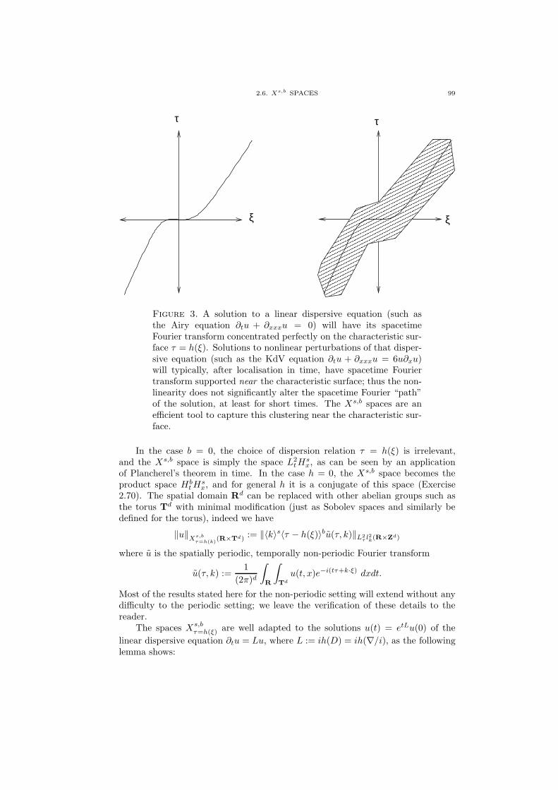
2.6. Xs,b SPACES 99
τ
ξ ξ
τ
Figure 3. A solution to a linear dispersive equation (such asthe Airy equation ∂tu + ∂xxxu = 0) will have its spacetimeFourier transform concentrated perfectly on the characteristic sur-face τ = h(ξ). Solutions to nonlinear perturbations of that disper-sive equation (such as the KdV equation ∂tu + ∂xxxu = 6u∂xu)will typically, after localisation in time, have spacetime Fouriertransform supported near the characteristic surface; thus the non-linearity does not significantly alter the spacetime Fourier “path”of the solution, at least for short times. The Xs,b spaces are anefficient tool to capture this clustering near the characteristic sur-face.
In the case b = 0, the choice of dispersion relation τ = h(ξ) is irrelevant,and the Xs,b space is simply the space L2
tHsx, as can be seen by an application
of Plancherel’s theorem in time. In the case h = 0, the Xs,b space becomes theproduct space Hb
tHsx, and for general h it is a conjugate of this space (Exercise
2.70). The spatial domain Rd can be replaced with other abelian groups such asthe torus Td with minimal modification (just as Sobolev spaces and similarly bedefined for the torus), indeed we have
‖u‖Xs,bτ=h(k)
(R×Td) := ‖〈k〉s〈τ − h(ξ)〉bu(τ, k)‖L2τ l
2k(R×Zd)
where u is the spatially periodic, temporally non-periodic Fourier transform
u(τ, k) :=1
(2π)d
∫
R
∫
Td
u(t, x)e−i(tτ+k·ξ) dxdt.
Most of the results stated here for the non-periodic setting will extend without anydifficulty to the periodic setting; we leave the verification of these details to thereader.
The spaces Xs,bτ=h(ξ) are well adapted to the solutions u(t) = etLu(0) of the
linear dispersive equation ∂tu = Lu, where L := ih(D) = ih(∇/i), as the followinglemma shows:

100 2. CONSTANT COEFFICIENT LINEAR DISPERSIVE EQUATIONS
Lemma 2.8 (Free solutions lie in Xs,b). Let f ∈ Hsx(R
d) for some s ∈ R, andlet L = ih(∇/i) for some polynomial h : Rd → R. Then for any Schwartz timecutoff η ∈ Sx(R), we have
‖η(t)etLf‖Xs,bτ=h(ξ)
(R×Rd) .η,b ‖f‖Hsx(Rd).
Proof. A computation shows that the spacetime Fourier transform of η(t)etLf
at (τ, ξ) is simply η(τ − h(ξ))f(ξ). Since η is rapidly decreasing, the claim follows.
We now discuss the basic properties of the Xs,b spaces. We first observe theeasily verified fact that the Xs,b spaces are Banach spaces. We have the trivialnesting
Xs′,b′
τ=h(ξ) ⊂ Xs,bτ=h(ξ)
whenever s′ ≤ s and b′ ≤ b. From Parseval’s identity and Cauchy-Schwarz we havethe duality relationship
(Xs,bτ=h(ξ))
∗ = X−s,−bτ=−h(−ξ).
Also, these spaces interpolate nicely in the s and b indices, as can be seen using theStein complex interpolation theorem (see e.g. [Stei2]). These two facts can savesome effort when proving certain estimates regarding the Xs,b spaces, particularlythe multilinear estimates.
Now we study the invariance and stability properties of these spaces. The Xs,b
spaces are invariant under translations in space and time, but they are usually notinvariant under frequency modulations (e.g. multiplication by a spatial phase eix·ξ
or a temporal phase eitτ ). The behaviour under complex conjugation is given bythe identity
‖u‖Xs,bτ=−h(−ξ)
= ‖u‖Xs,bτ=h(ξ)
and thus one has conjugation invariance when h is odd, but not necessarily other-wise.
When b > 1/2, one can view the Xs,b spaces as being very close to free solutions(i.e. solutions to the equation ∂tu = Lu). This is formalised in the following lemma:
Lemma 2.9. Let L = iP (∇/i) for some polynomial P : Rd → R, let s ∈ R,and let Y be a Banach space of functions on R × Rd with the property that
‖eitτ0etLf‖Y . ‖f‖Hsx(Rd)
for all f ∈ Hsx(R
d) and τ0 ∈ R. Then we have the embedding
‖u‖Y .b ‖u‖Xs,bτ=h(ξ)
(R×Rd).
Conversely, free solutions will lie in Xs,b once suitably truncated in time; seeLemma 2.11.
Proof. By Fourier inversion we have
u(t, x) =1
(2π)d+1
∫
R
∫
Rd
u(τ, ξ)eitτ eix·ξ dξdτ.
If we write τ = h(ξ) + τ0, and set
fτ0(x) :=1
(2π)d
∫
Rd
u(h(ξ) + τ0, ξ)eix·ξ dξ

2.6. Xs,b SPACES 101
we have
etLfτ0(x) =1
(2π)d
∫
Rd
u(h(ξ) + τ0, ξ)eith(ξ)eix·ξ dξ
and thus have the representation
u(t) =1
2π
∫
R
eitτ0etLfτ dτ0.
Taking Y norms and using Minkowski’s inequality and the hypothesis on Y , weobtain
‖u‖Y .
∫
R
‖fτ0‖Hsx(Rd) dτ0,
and hence by Cauchy-Schwarz and the hypothesis b > 1/2
‖u‖Y .b(
∫
R
〈τ0〉2b
‖fτ0‖2Hs
x(Rd) dτ0)1/2.
Using Plancherel’s theorem, the right-hand side rearranges to equal Cb‖u‖Xs,b, andthe claim follows.
Observe that the same argument applies when P is merely a continuous functionrather than a polynomial, though in this case L will be a Fourier multiplier ratherthan a differential operator. Applying this to Y = C0
tHsx, we obtain the immediate
corollary
Corollary 2.10. Let b > 1/2, s ∈ R, and h : Rd → R be continuous. Then
for any u ∈ Xs,bτ=h(ξ)(R × Rd) we have
‖u‖C0tH
sx(R×Rd) .b ‖u‖Xs,b
τ=h(ξ)(R×Rd).
Furthermore, the Xs,b spaces enjoy the same Sobolev embeddings that freesolutions to the equation ut = Lu do. For instance, by combining Lemma 2.9 with(2.24) (and observing that the spaces LqtL
rx are invariant under multiplication by
phases such as eitτ0), one concludes that
‖u‖LqtL
rx(R×Rd) .q,r,b ‖u‖X0,b
τ=|ξ|2(R×Rd)
for all Schrodinger-admissible (q, r).It turns out that the Xs,b spaces are only well suited to analyzing nonlinear
dispersive equations when one localises in time. Fortunately, these spaces are easyto localise:
Lemma 2.11 (Xs,b is stable wrt time localisation). Let η ∈ St(R) be a Schwartzfunction in time. Then we have
‖η(t)u‖Xs,bτ=h(ξ)
(R×Rd) .η,b ‖u‖Xs,bτ=h(ξ)
(R×Rd)
for any s, b ∈ R, any h : Rd → R, and any field u ∈ St,x(R × Rd). Furthermore,if −1/2 < b′ ≤ b < 1/2, then for any 0 < T < 1 and σ > 0 we have
‖η(t/T )u‖Xs,b′
τ=h(ξ)(R×Rd)
.η,b,b′ Tb−b′‖u‖Xs,b
τ=h(ξ)(R×Rd).
The second estimate in this lemma is useful in the large data theory, as it allowsone to keep certain Xs,b norms of a solution small by localizing to a sufficientlysmall time interval.

102 2. CONSTANT COEFFICIENT LINEAR DISPERSIVE EQUATIONS
Proof. Let us first understand how the Xs,b spaces behave with respect totemporal frequency modulation u(t, x) 7→ eitτ0u(t, x). From the crude estimate
〈τ − τ0 − h(ξ)〉b .b 〈τ0〉|b|〈τ − h(ξ)〉b
and elementary Fourier analysis, we conclude that
‖eitτ0u‖Xs,bτ=h(ξ)
(R×Rd) .b 〈τ0〉|b|‖u‖Xs,bτ=h(ξ)
(R×Rd).
If we now use Fourier expansion in time to write η(t) =∫Rη(τ0)e
itτ0 dτ0 and useMinkowski’s inequality, we conclude
‖η(t)u‖Xs,bτ=h(ξ)
(R×Rd) .b (
∫
R
|η(τ0)|〈τ0〉|b| dτ0)‖u‖Xs,bτ=h(ξ)
(R×Rd).
Since η is Schwartz, η is rapidly decreasing, and the first claim follows.Now we prove the second claim. By conjugating by 〈∇〉s we may take s = 0.
By composition it suffices to treat the cases 0 ≤ b′ ≤ b or b′ ≤ b ≤ 0; by dualitywe may then take 0 ≤ b′ ≤ b. By interpolation with the trivial case b′ = b we maytake b′ = 0, thus we are now reduced to establishing
‖η(t/T )u‖L2tL
2x(R×Rd) .η,b T
b‖u‖X0,bτ=h(ξ)
(R×Rd)
for 0 < b < 1/2. By partitioning frequency space we can divide into two cases, onewhere u is supported on the region 〈τ−h(ξ)〉 ≥ 1/T , and one where 〈τ−h(ξ)〉 ≤ 1/T .In the former case we will have
‖u‖X0,0τ=h(ξ)
(R×Rd) ≤ T b‖u‖X0,bτ=h(ξ)
(R×Rd)
and the claim then follows from the boundedness of η. In the latter case, we use avariant of Corollary 2.10, noting for any time t that
‖u(t)‖L2x(Rd) . ‖u(t)(ξ)‖L2
ξ(Rd)
. ‖∫
〈τ−h(ξ)〉≤1/T
|u(τ, ξ)| dτ‖L2ξ(Rd)
.b Tb−1/2‖(
∫〈τ − h(ξ)〉2b|u(τ, ξ)|2 dτ)1/2‖L2
ξ(Rd)
= T b−1/2‖u‖Xs,bτ=h(ξ)
(R×Rd)
thanks to Plancherel, the triangle inequality, Cauchy-Schwarz, and the localisationof u. Integrating this against η(t/T ), the claim follows.
The Xs,b spaces react well to Fourier multipliers, in much the same way thatordinary Sobolev spaces Hs do. If Dk is a Fourier multiplier of order k, in the sensethat
Dkf(ξ) = m(ξ)f(ξ)
for all Schwartz functions f ∈ Sx(Rd) and some measurable multiplier m : Rd → C
obeying the growth condition |m(ξ)| . 〈ξ〉k, then D can be extended to spacetimefunctions by acting on each time separately, thus (Du)(t) = D(u(t)), or in terms ofthe spacetime Fourier transform
Dku(τ, ξ) = m(ξ)u(τ, ξ)
2.6. Xs,b SPACES 103
and then one easily verifies that D maps Xs,bτ=h(ξ) continuously to Xs−k,b
τ=h(ξ) for any
s, b ∈ R and any h:
‖Dku‖Xs−k,bτ=h(ξ)
. ‖u‖Xs,bτ=h(ξ)
.
This is analogous to the well-known estimate ‖Dku‖Hs−k . ‖u‖Hs for Sobolevspaces. In the case when k is a non-negative integer, we have the converse
(2.59) ‖u‖Xs,bτ=h(ξ)
. ‖u‖Xs−k,bτ=h(ξ)
+ ‖∇kxu‖Xs−k,b
τ=h(ξ),
which is proven by repeating the above arguments. Similarly, if h : Rd → R is apolynomial and L := ih(∇/i), then we have
˜(∂t − L)u(τ, ξ) = i(τ − h(ξ))u(τ, ξ)
and hence
‖(∂t − L)u‖Xs,b−1τ=h(ξ)
. ‖u‖Xs,bτ=h(ξ)
.
It is natural to ask whether there is a converse inequality, in the spirit of (2.59).This is indeed the case:
Proposition 2.12 (Xs,b energy estimate). Let h : Rd → R be a polynomial,let L := ih(∇/i), and let u ∈ C∞
t,locSx(R×Rd) be a smooth solution to the equation
ut = Lu + F . Then for any s ∈ R and b > 1/2, and any compactly supportedsmooth time cutoff η(t), we have
‖η(t)u‖Xs,bτ=h(ξ)
(R×Rd) .η,b ‖u(0)‖Hsx(Rd) + ‖F‖Xs,b−1
τ=h(ξ)(R×Rd).
Proof. To abbreviate the notation we shall write Xs,bτ=h(ξ)(R×Rd) simply as
Xs,b. Let [−R,R] be a time interval containing the support of η. By truncating Fsmoothly in time, using a compactly supported cutoff that equals 1 on [−R,R] wemay assume (using Lemma 2.11) that F is supported on [−2R, 2R] and is Schwartzin spacetime. Also, by applying 〈∇〉s to both u and F if necessary, we may takes = 0.
Let us first suppose that u vanishes at time −2R, thus u(−2R) = 0. ByDuhamel’s formula (2.13) (with t0 = −2R) we thus have
η(t)u(t) = η(t)
∫ t
−∞e(t−s)LF (s) ds = η(t)
∫
R
η(t− s)1[0,+∞)(t− s)e(t−s)LF (s) ds
where η is a smooth compactly supported function which equals 1 on [−3R, 3R].By Lemma 2.11, it would thus suffice to show that
‖∫
R
η(t− s)1[0,+∞)(t− s)e(t−s)LF (s) ds‖X0,b .η,b ‖F‖X0,b−1 .
A routine computation shows that the spacetime Fourier transform of∫Rη(t −
s)1[0,+∞)(t− s)e(t−s)LF (s) ds at (τ, ξ) is equal to
(
∫
R
η(t)1[0,+∞)(t)e−it(τ−h(ξ))dt)F (τ, ξ).
The expression inside the parentheses can be shown (via integration by parts) tobe at most Oη(〈τ − ξ〉−1). The claim then follows.

104 2. CONSTANT COEFFICIENT LINEAR DISPERSIVE EQUATIONS
Now we handle the general case. We split u(t) = (u(t) − e(t+2R)Lu(−2R)) +etLe2RLu(−2R). For the first term, the preceding argument applies, and we have
‖η(t)(u(t) − e(t+2R)Lu(−2R))‖X0,b(R×Rd) .η,b ‖F‖X0,b .
Thus it will suffice to control the remaining term. Applying Lemma 2.8, it thussuffices to show that
‖e2RLu(−2R)‖L2x
.η,b ‖u(0)‖L2x
+ ‖F‖X0,b−1 .
From Duhamel’s formula and the support of F we have
e2RLu(−2R) = u(0) +
∫
R
η(s)1(−∞,0](s)e−sLF (s) ds
where η is as before. Thus by the triangle inequality it suffices to show that
‖∫
R
η(s)1(−∞,0](s)e−sLF (s) ds‖L2
x.η,b ‖F‖X0,b−1 .
Applying Parseval’s identity, the left-hand side can be written as
‖∫
R
(
∫
R
η(s)1(−∞,0](s)eis(τ−h(ξ)) ds)F (τ, ξ) dτ‖L2
ξ.
An integration by parts yields the bound∫
R
η(s)1(−∞,0](s)eis(τ−h(ξ)) ds| .η 〈τ − h(ξ)〉−1
and hence by Cauchy-Schwarz and the hypothesis b > 1/2 we have
|∫
R
(
∫
R
η(s)1(−∞,0](s)eis(τ−h(ξ)) ds)F (τ, ξ) dτ | .η,b |
∫
R
〈τ−h(ξ〉2(b−1)|F (τ, ξ)|2 dτ)1/2,
and the claim follows.
As observed earlier, Xs,b spaces enjoy all the Strichartz estimates that freesolutions do. However, in some cases, particularly in periodic settings, it is notalways easy to obtain Strichartz estimates, as dispersive inequalities are typicallynot available in periodic settings. (When the domain is compact, L∞
x decay isinconsistent with L2
x conservation.) However, if one is interested in L4t,x or L6
t,x
type inequalities, one can sometimes establish the Strichartz estimate by a directFourier-analytic approach. A typical result, which is of application to the periodicSchrodinger equation26 is as follows.
Proposition 2.13 (Periodic Schrodinger estimate). [Bou] We have
‖u‖L4tL
4x(R×T) . ‖u‖
X0,3/8
τ=k2(R×T).
for any u ∈ St,x(R × T).
26Depending on the choice of normalisation used for the Schrodinger equation, the dispersionrelation τ = h(k) may differ from τ = k2 by an absolute constant, but this makes no differenceto this Strichartz estimate. Note however that for bilinear estimates one needs to distinguish theXs,b space associated to τ = k2 from the conjugate Xs,b space, associated with τ = −k2.

2.6. Xs,b SPACES 105
Proof. We use an argument of Nikolay Tzvetkov. Split u =∑
M uM , whereM ranges over integer powers of 2, and uM is the portion of u localised to thespacetime frequency region 2M ≤ 〈τ − k2〉 < 2M+1. From Plancherel’s theorem wehave ∑
M
M3/4‖uM‖2L2
tL2x(R×T) . ‖u‖2
X0,3/8
τ=k2(R×T)
Squaring both sides of the desired inequality and using the triangle inequality, wereduce to proving that
∑ ∑
M≤M ′
‖uMuM ′‖L2tL
2x(R×T) .
∑
M
M3/4‖uM‖2L2
tL2x(R×T).
Setting M ′ = 2mM , it thus suffices by the triangle inequality to prove that∑
M
‖uMu2mM‖L2tL
2x(R×T) . 2−εm
∑
M
M3/4‖uM‖2L2
tL2x(R×T)
for all m ≥ 0 and some absolute constant ε > 0; by Cauchy-Schwarz it thus sufficesto establish that
‖uMu2mM‖L2tL
2x(R×T) . 2−εmM3/8‖uM‖L2
tL2x(R×T)(2
mM)3/8‖u2mM‖L2tL
2x(R×T).
Let us now normalise uM and u2mM to have L2tL
2x norm one. We use Plancherel
and reduce to showing
‖∑
k1+k2=k
∫
τ1+τ2=τ
uM (τ1, k1)u2mM (τ2, k2) dτ1‖L2τ l
2k(R×Z) . 2(3/8−ε)mM3/4.
On the other hand, from the normalisation and Fubini’s theorem we have
‖(∑
k1+k2=k
∫
τ1+τ2=τ
|uM (τ1, k1)|2|u2mM (τ2, k2)|2 dτ1)1/2‖L2τ l
2k(R×Z) = 1
so by Cauchy-Schwarz and the support of uM , u2mM it will suffice to show that
∑
k1+k2=k
∫
τ1+τ2=τ ;τ1=k21+O(M);τ2=k2
2+O(2mM)
1 dτ1 . 2(3/4−2εm)M3/2
for all k, τ .Fix k, τ . Observe that for the integral to be non-empty, we must have τ =
k21 + k2
2 + O(2mM), in which case the integral is O(M). Thus it suffices to showthat ∑
k1+k2=k;τ=k21+k2
2+O(2mM)
1 . 2(3/4−2ε)mM1/2.
But if τ = k21 +k2
2 +O(2mM) and k1 +k2 = k, then (k1−k2)2 = 2τ −k+O(2mM),
and hence k1 − k2 is constrained to at most two intervals of length O(2m/2M1/2).The claim then follows with ε = 1/8.
In Section 4.1 we shall encounter some bilinear and trilinear Xs,b estimates ina spirit similar to the above (see also the exercises below).
Exercise 2.70 (Xs,b vs. product Sobolev spaces). Let u ∈ S(R × Rd) be acomplex field and let h : Rd → R be a polynomial. Let U(t) := exp(ith(∇/i))be the linear propagators for the equation ut = Lu, where L = ih(∇/i). Let
106 2. CONSTANT COEFFICIENT LINEAR DISPERSIVE EQUATIONS
v : R × Rd → C be the function v(t) := U(−t)u(t), thus v is constant in time ifand only if u solves the equation ut = Lu. Show that
‖v‖Xs,bτ=h(ξ)
(R×Rd) = ‖u‖HbtH
sx(R×Rd)
for all s, b ∈ R.
Exercise 2.71 (Endpoint Xs,b spaces). Show that Lemma 2.9, Corollary 2.10,Lemma 2.11, and Proposition 2.12 all break down at the endpoint b = 1/2. (Butsee the next exercise.)
Exercise 2.72 (Endpoint Xs,b spaces, II). Let h : Zd → R, and let s, b be
real numbers. Define the space Y s,bτ=h(k)(R × Td) to be the closure of the Schwartz
functions under the norm
‖u‖Y s,bτ=h(k)
(R×Td) := ‖〈k〉s〈τ − h(k)〉bu‖l2kL1τ (R×Zd).
Establish the embeddings
‖u‖Y
s,b−1/2−ε
τ=h(k)(R×Td)
.ε ‖u‖Xs,bτ=h(k)
(R×Td)
and
‖u‖C0tH
sx(R×Td) . ‖u‖Y s,0(R×Td)
for all Schwartz functions u and all ε > 0; show that the former embedding breaksdown at ε = 0. With the notation of Proposition 2.12, establish the energy estimate
‖η(t)u‖Y s,0τ=h(ξ)
(R×Td) + ‖η(t)u‖X
s,1/2
τ=h(ξ)(R×Td)
.η,b (‖u(0)‖Hsx(Td) + ‖F‖Y s,−1
τ=h(ξ)(R×Td) + ‖F‖
Xs,−1/2
τ=h(ξ)(R×Td)
).
In the periodic theory, these estimates allow one to use the endpoint space Xs,1/2
(which is otherwise very badly behaved, as the preceding exercise showed) by aug-menting it with the additional space Y s,0.
Exercise 2.73 (Xs,b spaces for the wave equation). Let us work in Minkowskispace R1+d with c = 1. Define the norm ‖u‖s,b := ‖u‖Xs,b
|τ|=|ξ|(R1+d) by
‖u‖s,b := ‖〈ξ〉s〈|τ | − |ξ|〉bu‖L2(R1+d).
Also define the slightly stronger norm X s,b by
‖u‖X s,b := ‖u‖s,b + ‖∂tu‖s−1,b.
Develop analogues of Corollary 2.10 and Lemma 2.11. Establish that
‖u‖s−1,b−1 .s,b,d ‖u‖X s,b
for all u ∈ St,x(R1+d), and conversely that one has the energy estimate
‖η(t)u‖X s,b .s,b,η (‖u(0)‖Hsx(Rd) + ‖∂tu(0)‖Hs−1
x (Rd) + ‖u‖s−1,b−1)
for all compactly supported bump functions η, all u ∈ St,x(R1+d), all s ∈ R, andall b > 1/2. Typically, in applications one would place the solution u in the space
X s,b and the nonlinearity u in Xs−1,b−1|τ |=|ξ| . What is the counterpart of Lemma 2.9?
2.6. Xs,b SPACES 107
Exercise 2.74. Let u ∈ St,x(R × T2) solve the inhomogeneous Schrodingerequation i∂tu+ ∆u = F . Show that
‖η(t)u‖C0tL
4x(R×T2) + ‖η(t)u‖L4
t,x(R×T2) .η ‖u(0)‖L2x(T2) + ‖F‖
L4/3t,x (R×T2)
for all compactly supported cutoff functions η. (Hint: use Proposition 2.13 and theChrist-Kiselev lemma, Lemma 2.4.)
Exercise 2.75 (Bilinear refinement to Strichartz). [Bou9], [CKSTT11] Letu, v ∈ St,x(R×Rd) be fields whose spacetime Fourier transforms u, v are supportedon the sets |ξ| ≤ M and |ξ| ≥ N respectively for some N,M ≥ 1. If d = 1, let usimpose the additional hypothesis N > 2M . Show that
‖uv‖L2tL
2x(R×Rd) .b
M (d−1)/2
N1/2‖u‖X0,b
τ=|ξ|2(R×Rd)‖v‖X0,b
τ=|ξ|2(R×Rd).
(Hint: use Lemma 2.9 twice to reduce u and v to free solutions of the Schrodingerequation, and compute using Plancherel explicitly. In the case d = 2 and N ≤ 2M ,one can use Strichartz estimates.)
Exercise 2.76 (Divisor bound). Show that a positive integer d has at mostOε(n
ε) divisors for any ε > 0. (Hint: first show that if d is the power of a primep, then d has at most Oε(n
ε) divisors, and in fact has at most nε divisors if p issufficiently large depending on ε. For the general case, factorise d into the productof prime powers.)
Exercise 2.77 (Periodic Airy L6t,x estimate). [Bou] Using Exercise 2.76 and
the identity
(k1 + k2 + k3)3 − k3
1 − k32 − k3
3 = 3(k1 + k2)(k2 + k3)(k3 + k1),
show that for any integers k, t that the number of integer solutions to the systemk1 + k2 + k3 = k, k3
1 + k32 + k3
3 = t with k1, k2, k3 = O(N) is at most Oε(Nε) for
any N ≥ 1 and ε > 0. Use this to obtain the estimate
‖∑
k∈Z
akeikx+ik3t‖L2
tL2x(T×T) .ε (
∑
k∈Z
〈k〉εa2k)
1/2
for any complex numbers ak and any ε > 0, and use this in turn to conclude theStrichartz estimate
‖η(t)u‖L6tL
6x(R×T) .ε,b ‖u‖Xε,b
τ=k3(R×T)
for any ε > 0 and b > 1/2 and any field u. It would be of interest to know if thisestimate holds for ε = 0, or with the exponent p = 6 replaced by a larger exponentsuch as p = 8.
Exercise 2.78 (Periodic Airy L6 estimate, II). [Bou] Show that for any in-tegers k, t that the number of integer solutions to the system k1 + k2 − k3 = k,k21 +k2
2 −k23 = t with k1, k2, k3 = O(N) is at most Oε(N
ε) for any N ≥ 1 and ε > 0.(Hint: use the first equation to eliminate k3 from the second, and then obtain anidentity of the form (k1 + a)(k2 + b) = c for some a, b, c given explicitly in terms ofk, t.) By arguing as in the preceding exercise, show that
‖η(t)u‖L6tL
6x(R×T) .ε,b ‖u‖Xε,b
τ=k2(R×T)
for any ε > 0 and b > 1/2 and any field u. It is known that the ε cannot be setto zero in this case, though perhaps if the exponent p = 6 were lowered slightly

108 2. CONSTANT COEFFICIENT LINEAR DISPERSIVE EQUATIONS
then this could be possible. See also [CKSTT3], [CKSTT12] for some trilinearrefinements of this estimate in which the ε loss can be eliminated.

CHAPTER 3
Semilinear dispersive equations
Come what come may,Time and the hour runs through the roughest day.(William Shakespeare, “Macbeth”)
In this chapter we turn at last to the main subject of this monograph, namelynonlinear dispersive equations. Specifically, we now study the local and globallow-regularity wellposedness of the following two Cauchy problems: the nonlinearSchrodinger equation (NLS)1
iut +1
2∆u = µ|u|p−1u
u(t0, x) = u0(x) ∈ Hsx(R
d)(3.1)
and the nonlinear wave equation (NLW)
u = µ|u|p−1u
u(t0, x) = u0(x) ∈ Hsx(R
d)
∂tu(t0, x) = u1(x) ∈ Hs−1(Rd).
(3.2)
In this chapter we have normalised c = ~ = m = 1, so that = −∂2t + ∆. We
will often also take advantage of time translation invariance to normalise t0 = 0.In both cases, the scalar field u : R1+d → C (or u : I × Rd → C, if one onlyseeks local solutions) is the desired solution, and the initial data u0 (and u1, in thecase of NLW) is specified and lies in a given Sobolev space Hs
x(Rd) (or Hs−1
x (Rd)).The exponent 1 < p < ∞ denotes the power of the nonlinearity and is also given;the sign µ ∈ −1, 0,+1 denotes whether the nonlinearity is defocusing, absent, orfocusing respectively2; we will see some reasons for this terminology later in thischapter. The cases when p is an odd integer, and in particular the cubic case p = 3and the quintic case p = 5, are particularly important in mathematical physics,and have the advantage that the nonlinearity z 7→ |z|p−1z is smooth, indeed it is apolynomial in z and z. We shall refer to these instances of NLS and NLW as thealgebraic NLS and NLW respectively. The periodic analogues of these problems,when the domain is the torus Td instead of Euclidean space Rd is also of interest,though our main focus here shall be on the non-periodic case.
1The factor of 12
can be easily eliminated by rescaling time by a factor of 2, and so can be
safely ignored. We retain it in order to make the dispersion relation (or de Broglie law) betweenvelocity and frequency as simple as possible, namely v = ξ.
2The defocusing and focusing nonlinearities are sometimes called repulsive and attractivenonlinearities in the literature.
109

110 3. SEMILINEAR DISPERSIVE EQUATIONS
For the NLW it is convenient to adopt the notation u[t] := (u(t), ∂tu(t)), thusfor instance u[t0] = (u0, u1). Thus u[t] describes the total state (both position andvelocity) of the solution u at time t.
The power-type nonlinearity function F (u) := µ|u|p−1u can be replaced byother nonlinearities, and in many cases one obtains results similar to those statedhere. But the specific choice of power-type nonlinearity has a number of niceproperties that make it well-suited for exposition, in particular enjoying symmetriessuch as the scaling and phase rotation symmetry F (zu) = |z|pF (u) for any complexz, which will in turn lead to corresponding symmetries for NLS and NLW. It isalso naturally associated to a Hamiltonian potential V (u) := 1
p+1µ|u|p+1 via the
observationd
dεV (u+ εv)|ε=0 = Re(F (u)v)
for any u, v ∈ C; this will lead to a Hamiltonian formulation for NLS and NLW(Exercise 3.1).
We will be particularly interested in the low regularity problem: whether onestill has existence and uniqueness of solutions even when the initial datum onlylies in a very low Sobolev space. There are a number of reasons why one wouldwant to go beyond high-regularity (classical) solutions and consider low-regularityones3. Firstly, a good low-regularity theory gives more control on the nature ofsingularities of a solution, if they do indeed form; generally speaking, if one hasa local wellposedness theory in Hs
x, then that implies that a singularity can onlyform by making the Hs
x norm go to infinity (or to concentrate at a point, if thenorm Hs
x is critical with respect to scaling). Secondly, many of the key structuralfeatures of an equation - such as the conserved Hamiltonian, the symplectic form,the scale invariance, or other conserved or monotone quantities - are typically as-
sociated to rather low regularities such as L2x, H
1/2x , or H1
x, and in order to fullyexploit these features it is often important to have a good local theory at those reg-ularities. Thirdly, the technical challenge of working at low regularities (especiallynear or at the critical regularity) enforces a significant discipline on one’s approachto the problem - requiring one to exploit the structural properties of the equationas efficiently and as geometrically as possible - and has in fact led to the develop-ment of powerful and robust new techniques and insights, which have provided newapplications even for smooth solutions (for instance, in clarifying the dynamics ofenergy transfer between low and high frequencies). Finally, the task of extending alocal existence result to a global existence result can (somewhat paradoxically) beeasier if one is working at low regularities than high regularities, particularly if oneis working at the scale-invariant regularity, or a regularity associated to a conservedquantity.
The nonlinear Schrodinger and wave models (3.1), (3.2) are among the simplestnonlinear perturbations of the free (linear) Schrodinger and wave equations4. Bothequations are semilinear (the nonlinearity is lower order than the linear terms),
3Alternatively, one can continue to work exclusively with classical solutions so that there isno difficulty justifying various formal computations, but demand that all estimates depend onlyon low-regularity norms of the solution. In practice, the two approaches are essentially equivalent;in most cases one can use limiting arguments to recover the former from the latter.
4Indeed, the NLS (together with the KdV equation) frequently arises in physics as the firstnonlinear approximation of a dispersive system, by performing a Taylor expansion of the nonlin-earity and discarding all but the first term. See for instance [SSul].

3. SEMILINEAR DISPERSIVE EQUATIONS 111
and furthermore the nonlinear term contains no derivatives or non-local terms.Furthermore, these nonlinear equations retain many of the symmetries and struc-ture of their linear counterparts; for instance, the NLS is a Hamiltonian equationwith conservation of mass (charge), momentum, energy, enjoys scaling, Galilean,translation, and (partial) pseudoconformal symmetries, and enjoys several mono-tonicity formulae, including some of virial and Morawetz type. The NLW is alsoHamiltonian with a conserved stress-energy tensor, with all its attendant conse-quences such as Morawetz inequalities and finite speed of propagation, and alsoenjoys scaling, Lorentz, translation and (partial) conformal symmetries. On theother hand, these equations are not completely integrable (with the notable excep-tion of the one-dimensional cubic (p = 3) NLS, as well as a variant of the NLWknown as the sine-Gordon equation), and so do not admit many explicit solutions(beyond some standard solutions such as the ground state solitons). The largenumber of parameters present in these equations (the dimension n, the power p,the sign µ, the regularity s, and whether one wishes to consider periodic or non-periodic solutions) means that these equations exhibit a wide range of phenomenaand behaviour, and in many ways are quite representative of the much larger classof nonlinear dispersive and wave equations which are studied in the literature. Thuswhile our understanding of these equations is somewhat better than for most othernonlinear dispersive models (particularly for subcritical and critical regularities, forsmall data, and for the defocusing regularity), they are still so rich in structure andproblems that there is still plenty to be understood.
Broadly speaking, there are two major classes of techniques one can use to ana-lyze these equations. On the one hand, one has perturbative methods, which approx-imate the nonlinear equations (3.1), (3.2) by more tractable and well-understoodequations such as5 the free (and linear) Schrodinger or wave equations. The er-ror between the actual equation and the approximate equation is usually treatedby some sort of iteration argument (usually based on Duhamel’s formula) or bya Gronwall inequality argument (usually based on energy estimates). Another re-lated example of a perturbative method arises when constructing exact solutionsto NLS and NLW by first starting with an approximate solution (that solves theequation up to a small error) and then constructing some sort of iterative schemeor Gronwall inequality argument to convert the approximate solution to an exactone.
As the name implies, perturbative methods only work when the solution isvery close to its approximation; typically, this requires the initial datum to besmall (or a small perturbation of a special initial datum), or the time interval tobe small (or perhaps some spacetime integral of the solution to be well controlledon this time interval). When dealing with large solutions over long times, per-turbative techniques no longer work by themselves, and one must combine themwith non-perturbative methods. Examples of such methods include conservationlaws, monotonicity formulae, and algebraic transformations of the equation. Suchmethods are initially only justified for smooth solutions, but can often be extendedto rough solutions by means of the perturbative theory. Thus, global control of asolution is often obtained via a collaboration between the perturbative techniques
5In some cases one will use a more complicated equation as the approximating equation. Forinstance, if one is analyzing the NLS or NLW near a special solution such as a soliton solution,one often uses the linearised equation around that soliton as the approximating equation.

112 3. SEMILINEAR DISPERSIVE EQUATIONS
and non-perturbative techniques; typically, the perturbative theory guarantees awell-behaved solution provided that certain integrals of the solution stay bounded,and the non-perturbative theory guarantees control of these integrals provided thatthe solution remains well-behaved (see e.g. Figure 7.). This basic division of labouralready works remarkably well in many situations, although in some recent results(most notably in those employing the induction on energy strategy, see Chapter 5)one has had to apply a more advanced scheme.
We conclude this introduction by describing some special (and very explicit)solutions to both (3.1) and (3.2), in order to build some initial intuition aboutthese equations, though we emphasise that for generic initial data we do not expectany similarly explicit formula for the solution. Let us begin by using the classicalmethod of separation of variables, using solutions of ODE to construct specialsolutions to PDE. For any ξ ∈ Rd, the plane wave eix·ξ is an eigenfunction of theLaplacian ξ, and also has magnitude one, which leads one to consider the ansatz
(3.3) u(t, x) = eix·ξv(t).
Simple calculation then shows that in order to solve the NLS (3.1), v must obeythe ODE
∂tv = −i( |ξ|2
2+ µ|v|p−1)v
and to solve the NLW (3.2), v must obey the ODE
(3.4) ∂2t v = −(|ξ|2 + µ|v|p−1)v.
In the case of NLS, the ODE for v can be explicitly solved, leading to the planewave solutions
(3.5) u(t, x) := αeiξ·xei|ξ|2t/2eiµ|α|
p−1t
for any α ∈ C and ξ ∈ Zd. Note how the time oscillation of ei|ξ|2t/2 arising from
the linear evolution is augmented by the additional time oscillation eiµ|α|p−1t. In
the defocusing case µ = +1, both time oscillations are anti-clockwise, so one canview the defocusing nonlinearity as amplifying the dispersive effect of the linearequation; in the focusing case the focusing nonlinearity is instead trying to cancelthe dispersive effect. If the amplitude α is small compared the frequency ξ thenthe dispersive effect is stronger, but when the amplitude is large then the focusingeffect takes over. This already illustrates one useful heuristic: the focusing anddefocusing equations behave similarly when the initial data is small or when thefrequency is very large6.
As for the NLW (3.2), one can obtain a similar class of (complex) explicitsolutions
u(t, x) := αeiξ·xe±i(|ξ|2+µ|α|p−1)1/2t
provided that |ξ|2+µ|α|p−1 ≥ 0. This latter condition is automatic in the defocusingcase µ = +1 or the linear case µ = 0, but requires either the frequency ξ to belarge or the amplitude α to be small in the focusing case µ = −1. This is againconsistent with the heuristic mentioned earlier. When the initial data is large and
6Actually, this heuristic is only valid in “subcritical” situations, in which the high frequencies
scale more favourably than the low frequencies. In critical cases, the high and low frequencies areequally sensitive to the distinction between focusing and defocusing; the supercritical cases arevery poorly understood, but it is believed that the high frequency behaviour is radically differentin the focusing and defocusing cases.
3. SEMILINEAR DISPERSIVE EQUATIONS 113
positive compared to the frequency, then the ODE (3.4) can blow up (this can beseen for instance using Exercise 1.25, in the case when v is real); one explicit familyof blowup solutions in the focusing case µ = −1 (with ξ = 0) is given by
(3.6) u(t, x) := cp(t0 − t)−2/(p−1)
for t < t0, where cp := (2(p+1)(p−1)2 )1/(p−1) and t0 ∈ R is an arbitrary parameter. In
contrast, in the defocusing or linear cases µ = +1, 0 no blowup solution of the form(3.3) is possible, because (3.4) enjoys a coercive Hamiltonian7
H(v, ∂tv) =1
2|∂tv|2 +
1
2|ξ|2|v|2 +
µ
p+ 1|v|p+1
and thus (by Exercise 1.29) the solutions (3.3) will stay globally bounded for alltime. Similarly in the focusing case if the initial data is very small compared to thefrequency. Thus we see that the large data focusing behaviour is quite bad whencompared to the defocusing or linear cases.
The solutions of the form (3.3) have no decay in space and so will not lie inSobolev spaces such asHs
x(Rd), although if the frequency ξ lies in the integer lattice
Zd then we can view these solutions as lying in the periodic Sobolev spaces Hsx(T
d)for any s. In the (focusing) non-periodic case it is possible to create a different classof solutions by choosing an ansatz which oscillates in time rather than in space:
(3.7) u(t, x) = Q(x)eitτ ,
where ω ∈ R. This leads to the ground state equation
(3.8) ∆Q+ α|Q|p−1Q = βQ
where (α, β) := (−2µ, 2τ) for NLS and (α, β) := (−µ, τ2) for NLW. In the defocus-ing case we can take α, β > 0 (choosing τ to be positive). From Appendix B wethen recall that if 1 < p < ∞ is energy-subcritical in the sense that d
2 − 2p−1 < 1,
then there exists a smooth, positive, rapidly decreasing solution Q ∈ Sx(Rd) to theequation (3.8). This leads to the standard ground state soliton solution to eitherNLS or NLW associated to the temporal frequency τ > 0; it lies in every spatialSobolev spaceHs
x(Rd), and has a very simple behaviour in time. In the next section
we will apply the symmetries of NLW and NLS to generate further ground statesolitons. These solitons are only available in the focusing case; In Section 3.5 weshall establish Morawetz inequalities which show that nothing remotely resemblinga soliton can occur in the defocusing equation.
Exercise 3.1. Obtain the analogue of Exercise 2.47 for the NLS, and Exercise2.58 for the NLW, by adding the nonlinear potential energy term V (u) to theHamiltonian.
Exercise 3.2. Let u ∈ C2t,x,loc(R × Rd → V ) be a classical solution to a
d-dimensional NLS. Show that the field v ∈ C2t,x,loc(R × Rd+1 → V ) defined by
v(t, x1, . . . , xd, xd+1) := e−i(t+xd+1)u(t− xd+1
2, x1, . . . , xd)
is a classical solution to the corresponding d + 1-dimensional NLW (cf. Exercise2.11). This correspondence may help explain why many of the algebraic expressions
7The case µ = ξ = 0 is degenerate coercive, but this case can be treated by hand, leading tosolutions of linear growth in time.

114 3. SEMILINEAR DISPERSIVE EQUATIONS
defined below for the NLW have a counterpart for NLS, but with d replaced byd+ 1. This correspondence is less useful for the Hs
x wellposedness theory, becausethe functions v constructed above will not have finite Hs
x norm. One should alsocaution that this correspondence does not link periodic NLS solutions with periodicNLW solutions.
Exercise 3.3. By taking formal limits of the Lax pair formulation of theperiodic Ablowitz-Ladik system as discussed in Section 1.7, discover a Lax pairformalism for the one-dimensional cubic defocusing Schrodinger equation (in eitherthe periodic or nonperiodic settings).
3.1. On scaling and other symmetries
It has long been an axiom of mine that the little things are infin-itely the most important. (Sir Arthur Conan Doyle, “A Case ofIdentity”)
We now describe the concrete symmetries of NLS and NLW; to avoid technical-ities let us just work with classical solutions for now (we will discuss more generalnotions of solution in the next section). The NLS (3.1) enjoys the scaling symmetry
(3.9) u(t, x) 7→ λ−2/(p−1)u(t
λ2,x
λ); u0(x) 7→ λ−2/(p−1)u0(
x
λ)
for any dilation factor λ > 0 (thus time has twice the dimensionality of space), andthe Galilean invariance
(3.10) u(t, x) 7→ eix·ve−it|v|2/2u(t, x− vt); u0(x) 7→ eix·vu0(x)
for any velocity v ∈ Rd (cf. Exercise 2.5). It also enjoys the more mundane sym-metries of time translation invariance, space translation invariance, spatial rotationsymmetry, phase rotation symmetry u 7→ eiθu, as well as time reversal symmetry
u(t, x) 7→ u(−t, x); u0(x) 7→ u0(x).
In the pseudo-conformal case p = pL2 := 1 + 4d , one also use Exercise 2.28 to verify
the pseudo-conformal symmetry
(3.11) u(t, x) 7→ 1
(it)d/2u(
1
t,x
t)ei|x|
2/2t
for times t 6= 0. This symmetry is awkward to use directly (at least when t0 = 0)because of the singularity at t = 0; one typically uses the time translation and timereversal symmetries to move the singularity elsewhere (e.g. to the time t = −1).
Similarly, the NLW (3.2) enjoys the scaling symmetry
u(t, x) 7→ λ−2/(p−1)u(t
λ,x
λ);
u0(x) 7→ λ−2/(p−1)u0(x
λ);
u1(x) 7→ λ−2/(p−1)−1u1(x
λ)
(3.12)
for any dilation factor λ > 0 (thus time and space have equal dimension), and (ifthe solution exists globally in time) the Lorentz invariance
(3.13) u(t, x) 7→ u(t− v · x√1 − |v|2
, x− xv +xv − vt√1 − |v|2
)
3.1. ON SCALING AND OTHER SYMMETRIES 115
for all sub-luminal velocities v ∈ Rd with |v| < 1 (cf. Exercise 2.6); note that theeffect of this invariance on the initial data u0, u1 is rather complicated and requiressolving the equation (3.2). The NLW also enjoys spacetime translation invariance,spatial rotation symmetry, phase rotation symmetry, conjugation symmetry, andtime reversal symmetry. In the conformal case p = p
H1/2x
= 1 + 4d−1 , one also has
the conformal symmetry
u(t, x) 7→ (t2 − |x|2)−(d−1)/2u(t
t2 − |x|2 ,x
t2 − |x|2 )
inside the light cone |t| < |x|, thanks to Exercise 2.14.Unlike the Galilean invariance (3.10), the Lorentz invariance (3.13) has the
effect of time dilation - solutions which would ordinarily exhibit some special be-haviour (e.g. blowup) at a time T will instead do so at a much later time, typically
of the order of T/√
1 − |v|2. To compensate for this one can compose the Lorentz
transformation with the scaling transformation with λ := 1/√
1 − |v|2, leading tothe normalised Lorentz invariance
(3.14) u(t, x) 7→ (1 − |v|2)1/(p−1)u(t− v · x,√
1 − |v|2(x − xv) + xv − vt).
Symmetries have many uses. Through Noether’s theorem, they indicate whatconservation laws are available (though certain symmetries, particularly discreteones, do not necessarily yield a conservation law). They can give guidance as towhat type of techniques to use to deal with a problem; for instance, if one is trying toestablish wellposedness in a data class which is invariant under a certain symmetry,this suggests the use of estimates and other techniques which are also invariantunder that symmetry; alternatively, one can “spend” the symmetry by normalisingthe solution, for instance in making the solution centred or concentrated at theorigin (or some other specified location) in space, time, or frequency. If the dataclass is subcritical with respect to scaling, one can use the scaling symmetry totrade between time of existence and size of initial data; thus if one establishes alocal wellposedness at a fixed time (say up to time T = 1) for data with smallnorm, then one can often also establish local wellposedness at a small time forlarge data; typically the time of existence will be proportional to some negativepower of the norm of the data. Conversely, if the data class is supercritical withrespect to scaling (or more generally is lower than the invariant norm associatedto another symmetry), then it is likely that there is a significant obstruction toobtaining a wellposedness theory below that regularity, and one also expects thewellposedness theory at that regularity to be rather delicate. The reason for thisis that if the regularity is below the invariant regularity, then one can use thesymmetry to convert bad behaviour arising from large initial data at some timet > 0 to bad behaviour arising from small initial data at some time less than orequal to t, where “large” and “small” are measured with respect to the regularityHsx(R
d). Since large initial data would be expected to display bad behaviour veryquickly, one then expects to give examples of arbitrary small initial data whichdisplays bad behaviour arbitrarily quickly. This can often be used to contradictcertain types of wellposedness that one could hypothesise for this regularity. Seealso Principle 3.1 below.
Let us give some sample applications of the symmetry laws. The first is ablowup result for the pseudoconformal focusing NLS (so µ = −1 and p = pL2
x=
1+ 4d ). Recall that this equation has a soliton solution of the form u(t, x) = eitτQ(x)

116 3. SEMILINEAR DISPERSIVE EQUATIONS
for any τ > 0, where the ground state Q is a nonnegative Schwartz solution to theequation
∆Q+ 2Q1+4/d = 2τQ.
Applying the pseudoconformal transformation (3.11), we obtain the solution
(3.15)1
(it)d/2e−iτ/tei|x|
2/2tQ(x/t).
This solves the NLS equation for all times t 6= 0, and in fact lies in every Sobolevspace Hs
x(Rd) for such times, but blows up in a rather dramatic way as t → 0.
Thus the pseudoconformal focusing NLS can lead to blowup even from very smoothdecaying initial data, though we will later see that this is due to the initial datumbeing “large” in an L2
x(Rd) sense. This blowup occurs despite the solution being
bounded in L2x, and despite the conservation of the L2
x norm. Thus for PDE, apositive definite conservation law is not always sufficient to prevent blowup fromoccuring, in marked contrast to the situation for ODE; note that the solution (3.15)demonstrates rather vividly the lack of compactness of bounded subsets of L2
x(Rd).
Now consider a general NLS. Applying the pseudoconformal transformation inExercise 2.28, one no longer expects to recover the original equation; instead, thetransformed field v(t, x) will now obey the equation
(3.16) i∂tv + ∆v = td2 (p−pL2
x)µ|v|p−1v
for t 6= 0, where pL2x
:= 1 + 4d is the pseudoconformal power. We will analyze this
equation (3.16) in more detail later, but for now let us just extract a special classof solutions to (3.16) (and hence to NLS), by considering solutions v which areindependent of the spatial variable and thus simply solve the ODE
(3.17) i∂tv = td2 (p−pL2
x)µ|v|p−1v.
This ODE can be solved explicitly as
v(t, x) = α exp(− iµ|α|p−1
qtq)
for any α ∈ C and with q := d2 (p− pL2
x)+1, though in the critical-range case q = 0
(so p = 1 + 2d ) we have instead the solution
v(t, x) = α exp(−i|α|p−1 log |t|).We can of course invert the pseudoconformal transformation and obtain explicitsolutions to the original NLS for t 6= 0, namely
(3.18) u(t, x) =1
(it)d/2α exp(
i|x|22t
+iµ|α|p−1
qtq)
when q 6= 0 and
(3.19) u(t, x) =1
(it)d/2α exp(
i|x|22t
+ iµ|α|p−1 log |t|)
when q = 0. Of course when µ = 0 we recover the explicit solution u(t, x) =1
(it)d/2α exp( i|x|2
2t ) to the linear Schrodinger equation (essentially the fundamental

3.1. ON SCALING AND OTHER SYMMETRIES 117
solution8 for that equation). Comparison of these solutions yields the followingheuristic: as t → ±∞, the nonlinear Schrodinger equation should resemble thelinear Schrodinger equation when in the short-range case q > 0 (so p > 1 + 2
d ), but
not in the long-range9 case q < 0 or critical-range case q = 0 (though the divergencebetween the two equations should consist primarily of a phase shift, which shouldbe somehow “logarithmic” in the critical-range case). We will see some justificationof this heuristic later in this chapter, though our understanding here is far fromcomplete.
Now we observe some applications of the Galilean invariance law (3.10). Letus begin with a periodic NLS (with d, p and µ = ±1 arbitrary). In this periodicsetting we have the plane wave solutions
(3.20) uα,ξ(t, x) := αeiξ·xei|ξ|2t/2eiµ|α|
p−1t
for any ξ ∈ 2πZd and α ∈ C; one can view this as the Galilean transform of the
constant-in-space solutions αeiµ|α|p−1t. Suppose one fixes the frequency parameter
ξ to be large, and considers two distinct solutions uα,ξ, uα′,ξ of the above type with|α| ∼ |α′|. At time zero we have
‖uα,ξ(0)‖Hsx(Td), ‖uα′,ξ(0)‖Hs
x(Td) ∼ |α||ξ|s;‖uα,ξ(0) − uα′,ξ(0)‖Hs
x(Td) ∼ |α− α′||ξ|s
while at any later time t we have
‖uα,ξ(t)‖Hsx(Td), ‖uα′,ξ(t)‖Hs
x(Td) ∼ |α||ξ|s;‖uα,ξ(t) − uα′,ξ(t)‖Hs
x∼ |αeiµ|α|p−1t − α′eiµ|α
′|p−1t||ξ|s.Thus the Hs
x norms of the solutions uα,ξ and uα′,ξ do not change much in time, butthe Hs
x separation of these solutions can change due to a phase decoherence effect.Indeed we see that if |α| 6= |α′|, then there exists a time t ∼ |α|1−p for which the twophases become completely decohered, and ‖uα,ξ(t) − uα′,ξ(t)‖Hs
x(Td) ∼ |α||ξ|s. If s
is negative, then by taking α to be large and |ξ| to be comparable to (|α|/ε)−1/s, wecan construct for any δ, ε > 0, a pair of solutions uα,ξ, uα′,ξ to NLS of Hs
x(Td) norm
O(ε) and Hsx(T
d) norm separation O(δ) at time zero, such that at some later timet = O(ε) the Hs
x(Td) norm separation has grown to be as large as O(ε). This shows
that for negative s, a pair of solutions can separate in Hsx(T
d) norm arbitrarilyquickly; more precisely, the solution map u0 7→ u is not uniformly continuous fromHsx to C0
tHsx([0, T ] × Td) even for arbitrarily small T and for arbitrarily small
balls in Hsx(T
d). This is a negative result that rules out certain types of strongwellposedness results for the periodic NLS for negative Sobolev regularities.
8Indeed, one could view (3.18), (3.19) as the “nonlinear fundamental solution” for NLS.However these solutions are nowhere near as useful as the fundamental solution is for the linearequation, since we no longer have the principle of superposition in the nonlinear case and so wecannot build general solutions by superimposing translates of the fundamental solution. Never-theless, these explicit solutions provide some useful intuition as to the asymptotic behaviour ofthe equation for general data.
9The terminology here signifies the long-term strength of the nonlinearity and can be justifiedheuristically as follows. One can view the nonlinearity in NLS as a potential term with time-dependent potential µ|u|p−1. Assuming that the nonlinear evolution decays at the same rate as
the linear one, dispersive estimates suggest that |u| should decay like t−d/2. Thus we expect in theshort-range case we expect the potential to be integrable in time, which suggests by Gronwall’sinequality that the long-term effect of the nonlinearity is bounded.

118 3. SEMILINEAR DISPERSIVE EQUATIONS
One can run a similar argument for nonperiodic focusing NLS, by starting withthe ground state solution eitτQ(x), rescaling it by λ and then applying a Galileantransform to obtain the moving soliton solution
(3.21) uv,λ(t, x) 7→ λ−2/(p−1)ei(x·v+it|v|2/2+itτ/λ2
Q((x− vt)/λ)
for any v ∈ Rd and λ > 0; one can use these solutions to show that the solution mapto NLS (if it exists at all) is not uniformly continuous in Hs
x for certain low s; seeExercise 3.5. A similar result is also known for the defocusing case, replacing thesoliton solutions with another family of solutions that can be viewed as truncatedversions of the plane wave solutions (3.5); see Section 3.8.
Among all the symmetries, the scale invariance (3.9), (3.12) is particularly im-portant, as it predicts a relationship between time of existence and regularity ofinitial data. Associated to this invariance is the critical regularity sc := d
2 − 2p−1 .
Note that the scaling (3.9) preserves the homogeneous Sobolev norm ‖u0‖Hsc (Rd),
and similarly (3.12) preserves ‖u0‖Hsc (Rd) + ‖u1‖Hsc−1(Rd). The relationship be-
tween scaling and the inhomogeneous counterparts to these Sobolev norms is alittle more complicated, of course. We refer to regularities s > sc above the criticalnorm as subcritical, and regularities s < sc below the critical norm as supercrit-ical. The reason for this inversion of notation is that higher regularity data hasbetter behaviour, and thus we expect subcritical solutions to have less pathologi-cal behaviour than critical solutions, which in turn should be better behaved thansupercritical solutions. The other scalings also have their own associated regulari-ties; the Galilean symmetry and pseudoconformal symmetry preserve the L2
x(Rd)
norm, whereas the Lorentz symmetry and conformal symmetries are heuristicallyassociated to the H1/2(Rd) × H−1/2(Rd) norm (see Exercise 2.23).
In general, the relationship between the regularity Hsx of the initial data, the
scale-invariant regularity Hsc of the equation, the frequencies of the solution, andthe evolution of the solution tends to follow the following informal principles10:
Principle 3.1 (Scaling heuristic). Let u be a solution to either the NLS (3.1)or NLW (3.2), with initial position u0 in Hs
x (and initial velocity u1 in Hs−1, inthe case of the NLW).
(a) In the subcritical case s > sc, we expect the high frequencies of the solutionto evolve linearly for all time (unless a stronger obstruction than scalingexists). The low frequencies of the solution will evolve linearly for shorttimes, but nonlinearly for long times.
(b) In the critical case s = sc, we expect the high frequencies to evolve linearlyfor all time if their Hsc norm is small, but to quickly develop nonlinear be-haviour when the norm is large. (Again, we are assuming that no strongerobstruction to linear behaviour than scaling exists.) The low frequencies ofthe solution will evolve linearly for all time if their Hsc norm is small, but
10This principle should be taken with a grain of salt. On the one hand, it gives a goodprediction for those equations in which the scaling symmetry is in some sense “dominant”, andfor which the worst types of initial data are given by bump functions. On the other hand, there are
other situations in which other features of the equation (such as Galilean or Lorentz symmetries,or resonances) dominate, in which case instability can occur even when the scaling heuristicpredicts good behaviour. Conversely, some features of the equation, such as conservation laws ormonotonicity formulae, can provide more stability than the scaling heuristic predicts.

3.1. ON SCALING AND OTHER SYMMETRIES 119
will eventually develop nonlinear behaviour (after a long period of time)when the norm is large.
(c) In the supercritical case s < sc, the high frequencies are very unstable andwill develop nonlinear behaviour very quickly. The low frequencies are inprinciple more stable and linear, though in practice they can be quicklydisrupted by the unstable behaviour in the high frequencies. (This rela-tively good behaviour of the low frequencies is sometimes enough to obtaina weak solution to the equation, however, by using viscosity methods tosuppress the high frequencies; see Exercise 3.56.)
Let us now briefly give a heuristic discussion that lends some support to Prin-ciple 3.1. Let N > 0 be a frequency; frequencies N ≫ 1 correspond to highfrequencies, while frequencies N ≪ 1 correspond to low frequencies. A model ex-ample of an initial datum u0 of frequency ∼ N is a function which is supported ona ball B of radius 1/N , does not oscillate too much on this ball, and reaches anamplitude A on this ball. (For the NLW, one would also need to similarly specifyan initial velocity.) We will assume that this “rescaled bump function” example isthe “worst” type of initial data in the given class (i.e. bounded or small functionsin Hs
x or Hs−1); this assumption corresponds to the caveat given in the above prin-ciple that no stronger obstructions to linear behaviour exist than the scaling one.The L2
x norm of such a datum is roughly ∼ AN−d/2, and more generally (fromthe Fourier representation of the Hs
x norm) we expect the Hsx norm of this datum
to be ∼ ANs−d/2; thus if u0 is bounded in Hsx then A = O(Nd/2−s), and if u0
is small in Hsx then A ≪ Nd/2−s. Now, both the NLS (3.1) and the NLW (3.2)
contain a linear term ∆u and a nonlinear term µ|u|p−1u. On the ball B (at leastfor times close to 0), the linear term has magnitude ∼ N2A, while the nonlinearterm has amplitude ∼ Ap. If N2A ≫ Ap, we thus expect the linear term to dom-inate, and the solution should behave linearly (cf. Principle 1.37). If Ap ≫ N2A,we expect the nonlinear term to dominate and so one eventually expects nonlinear(and unstable) behaviour. The time in which this nonlinear behaviour becomesapparent can be predicted by comparing u against its time derivative ∂tu or itssecond time derivative ∂2
t u. For instance, suppose we have an NLS in which thenonlinear behaviour dominates, thus ∂tu will be dominated by the nonlinear termµ|u|p−1u, which has amplitude ∼ Ap. Since u itself has amplitude ∼ A, we expectthe nonlinear behaviour to significantly affect the initial datum after time ∼ A/Ap.Using these heuristics, one can give informal justification for all three components(a), (b), (c) if Principle 3.1; see Exercise 3.4.
A particular interesting case is when the scale-invariant regularity coincideswith one of the other special regularities, such as the H1
x norm (associated to
the energy or Hamiltonian), the H1/2x norm (associated to the momentum in NLS
and to the symplectic structure, Lorentz invariance, and conformal invariance inNLW), and the L2
x norm (associated to the Galilean invariance, pseudoconformalinvariance, and mass in NLS, and being the limiting regularity in NLW to evenmake sense of (3.2) distributionally); see Table 1. Thus we isolate as special cases
the H1x-critical (or energy-critical) case sc = 1 (thus d ≥ 3 and p = 1 + 4
d−2),
the H1/2x -critical case sc = 1/2 (thus d ≥ 2 and p = 1 + 4
d−1 ) and the L2x-critical
case sc = 0 (thus d ≥ 1 and p = 1 + 4d). One can also discuss the H1
x-subcritical
case sc < 1 and the H1x-supercritical case sc > 1, etc. Another relevant regularity

120 3. SEMILINEAR DISPERSIVE EQUATIONS
Table 1. The critical exponents for small dimension. The caseswhen a critical exponent corresponds to an algebraic equation (i.e.p is equal to 3 or 5) are of particular interest.
Dimension L2x-critical H
1/2x -critical H1
x-critical1 5 ∞ –2 3 5 ∞3 7/3 3 54 2 7/3 35 9/5 2 7/36 5/3 9/5 2
in the case of NLW is the Lorentz regularity sl := d+14 − 1
p−1 = sc
2 + 14 , which is
the regularity which is heuristically associated to the normalised Lorentz invariance(3.14), and is halfway between the scale-invariant regularity sc and the conformalregularity 1
2 .
Exercise 3.4. Use the heuristic analysis of bump function initial data, asdescribed in this section, to give some informal justification to Principle 3.1. (Beprepared to make a large number of hand-waving assumptions. The important thinghere is to develop the numerology of exponents; rigorous support for these heuristicswill be have to wait until later in this chapter.) In the subcritical case, develop aheuristic relationship between the Hs
x norm of the initial data and the predicted
time T in which the linear behaviour dominates. (One should get T ∼ ‖u0‖2/(s−sc)Hs
for NLS and T ∼ (‖u0‖Hs + ‖u1‖Hs−1)1/(s−sc) for the NLW.)
Exercise 3.5. [BKPSV] Let d, p be arbitrary, let µ = +1, and let s < 0 ors < sc := d
2− 2p−1 . Using the solutions (3.21), show that for any ε, δ > 0 there exists
a pair of classical solutions u, u′ to (3.1) with Hsx(R
d) norm O(ε) and Hsx(R
d) normseparation O(δ) at time zero, such that at some later time t = O(ε) the Hs
x(Rd)
norm separation has grown to be as large as O(ε). This shows that there is nouniform wellposedness at this regularity, at least for the focusing regularity.
3.2. What is a solution?
For every complex problem, there is a solution that is simple, neat,and wrong. (H.L. Mencken, “The Divine Afflatus”)
Before we begin the analysis of our model problems (3.1), (3.2), let us pauseto address a rather fundamental question, namely what it actually means for afield u to be a solution of either of these two Cauchy problems. This question maysound philosophical in nature, but the properties associated to making a solutionconcept “strong” are well worth establishing rigorously, as they become importantin establishing many of the further properties of the equation, such as the globalexistence and asymptotics of (classical) solutions.
The question of defining exactly what a solution is is more subtle than it mayfirst appear, especially at low regularities. The reason for this is that in orderfor a solution to a PDE to actually be useful for applications, it is not merely

3.2. WHAT IS A SOLUTION? 121
enough that it exist and solve the equation in some weak sense11 (e.g. in the senseof distributions), though this is certainly a minimal requirement; one also oftendesires additional properties on the solution, which do not automatically followfrom the fact that the equation is solved weakly. We informally describe some ofthe most important of these properties12 as follows.
• Existence: Is the solution guaranteed to exist (locally, at least) for allinitial data in a certain class (e.g. Hs
x)?• Uniqueness: Is the solution the unique object in a certain solution class
(e.g. C0tH
sx(I × Rd)) which solves the equation in a suitable sense (e.g.
in a distributional sense)? Is this solution concept compatible with othernotions of solution (i.e. if two solutions to the same equation exist in twodifferent senses, are they equal to each other)?
• Continuous dependence on the data: Do small perturbations of the initialdatum (in some norm) lead to small perturbations in the solution (insome other norm)? In other words, is the solution map continuous? Onecan also ask for stronger continuity properties such as uniform continuity,Lipschitz continuity, or analyticity.
• Bounds: If the initial datum is in some class, say Hsx, can one control
the solution in some other class, e.g. C0tH
sx(I × Rd)? In particular, does
one have persistence of regularity: is the solution always as smooth as theinitial datum (as measured in an Hs
x sense)?• Lifespan estimates: Is there a lower bound on the lifespan of the solution
in terms of the initial data (or in terms of some norm of the initial data,such as an Hs
x(Rd) norm)? Equivalently, is there a blowup criterion that
gives necessary conditions for the lifespan to shrink to zero? In some casesone has global existence, which case the lifespan is infinite.
• Approximability by smooth solutions: if the solution is rough, can it bewritten as the limit (in some topology) of smoother solutions? If theinitial datum is approximated by a sequence of smooth initial data, dothe corresponding solutions necessarily converge to the original solution,and in what sense?
• Stability: If one perturbs the equation (thus considering fields which onlysolve the original equation approximately), to what extent can these near-solutions be approximated by the exact solution with the same (or anearby) initial datum?
11This is in marked contrast with the theory of linear differential equations, in which dis-tributional solutions are very tractable, and can mostly be manipulated as if they were classicalsolutions, in large part because they can be expressed as the weak limit of classical solutions. Sinceweak convergence is often not preserved under basic nonlinear operations such as multiplication oftwo functions, one generally requires in nonlinear applications that a solution be a strong limit ofclassical solutions, which usually leads to the requirement that one work with wellposed solutions;see below.
12For elliptic PDE, another important property that one often desires is that the solution uis a minimiser, or at least a critical point, of the Lagrangian associated to the PDE, with respectto various classes of perturbation. One could insist on something similar for nonlinear wave andSchrodinger equations, but this has not proven to be as fruitful a property for these equations
as in the elliptic case, in large part because of the highly non-convex nature of the Lagrangiansinvolved. However, the Lagrangian formulation is (formally) linked to important properties suchas conservation laws and monotonicity formulae, which are very desirable properties for a solutionto obey.

122 3. SEMILINEAR DISPERSIVE EQUATIONS
• Structures: Do the conservation laws of the equation, which can be rigor-ously justified for classical (i.e. smooth and decaying) solutions, continueto hold for the solution class being studied? Similarly for monotonicityformulae, symmetries of the equation, etc.
Thus, instead of having a single unified concept of a solution class, one hasinstead a multi-dimensional continuum of such classes, ranging from very weaksolution classes (in which the equation solves the equation in a weak sense, oris perhaps a weak limit of smoother solutions or near-solutions, but not muchelse), to very strong solution classes, in which one has many or all of the desirableproperties listed above. Generally speaking, it is fairly easy to show existence ofsolution in a weak solution class by various limiting arguments (e.g. iteration orweak compactness arguments), but non-trivial effort is then required to upgradethose solutions to lie in stronger solution classes.
In this section we shall discuss five notions of solution, which in decreasing orderof strength are classical solution, wellposed Hs
x solution, strong Hsx solution, weak
Hsx solution, and distributional solution respectively. In fact, in this monograph we
shall largely work with wellposed and classical solutions, in order to avoid a numberof subtleties involving the weaker notions of solution.
To fix the discussion let us just work with the NLS equation (3.1), and fixour initial data class to be a Sobolev space Hs
x(Rd). The strongest notion of a
solution is that of a classical solution. These can (broadly speaking) be defined assolutions which have so much differentiability and decay that there is no difficultyinterpreting the problem (3.1) in a classical sense (i.e. without requiring the theoryof weak derivatives). Furthermore, one has enough regularity and decay available13
to justify all the various formal manipulations associated to the equation, such asconservation laws, monotonicity formulae, and so forth. The amount of regularityrequired to do all this can be quite large; for instance, in order to justify conser-vation of the Hamiltonian for NLS safely, one requires as much as three orders ofdifferentiability on the solution, as well as some additional uniformity and decayconditions. Because of this, one occasionally runs into issues generating a classi-cal solution theory when the nonlinearity µ|u|p−1u is not very smooth (which canhappen when p is close to 1); in such cases one may need to regularise the non-linearity before discussing classical solutions. However this issue does not arise forthe algebraic equations, in which p is an odd integer.
It is also easy to establish uniqueness for classical solutions (essentially becausethe proof of Theorem 1.14 carries over without difficulty). Here are two typicalsuch results, one for NLS and one for NLW.
Proposition 3.2 (Uniqueness for classical NLS solutions). Let I be a timeinterval containing t0, and let u, u′ ∈ C2
t,x(I × Rd → C) be two classical solutionsto (3.1) with the same initial datum u0 for some fixed µ and p. Assume also that wehave the mild decay hypothesis u, u′ ∈ L∞
t Lqx(I × Rd) for q = 2,∞. Then u = u′.
Proof. By time translation symmetry we can take t0 = 0. By time reversalsymmetry we may assume that I lies in the upper time axis [0,+∞). Let us writeu′ = u + v. Then v ∈ C2
t,x(I × Rd → C), v(0) = 0, and v obeys the difference
13This is a somewhat vague definition, but in practice we will always apply limiting argumentsto generalise classical solutions to a wider class of wellposed solutions, and so the exact notion ofa classical solution will not be important as long as it is dense in the class of wellposed solutions.

3.2. WHAT IS A SOLUTION? 123
equation
i∂tv + ∆v = µ(|u+ v|p−1(u+ v) − |u|p−1u).
Since v and |u+v|p−1(u+v)−|u|p−1u lie in L∞t L
2x(I×Rd), we may invoke Duhamel’s
formula (2.13) and conclude
v(t) = −iµ∫ t
0
ei(t−s)∆/2(|u+ v|p−1(u+ v) − |u|p−1u)(s) ds
for all t ∈ I. By Minkowski’s inequality, and the unitarity of ei(t−s)∆, we conclude
‖v(t)‖L2x(Rd) ≤
∫ t
0
‖(|u+ v|p−1(u+ v) − |u|p−1u)(s)‖L2x(Rd) ds.
Since u and v are in L∞t L
∞x (I × Rd), and the function z 7→ |z|p−1z is locally
Lipschitz, we have the bound
‖(|u+ v|p−1(u+ v) − |u|p−1u)(s)‖L2x(Rd) .p(‖u‖pL∞
t L∞x (I×Rd)
+ ‖v‖pL∞
t L∞x (I×Rd)
)
× ‖v(s)‖L2x(Rd).
Applying Gronwall’s inequality (Theorem 1.10) we conclude that ‖v(t)‖L2x(Rd) = 0
for all t ∈ I, and hence u = u′ as desired.
Note that Exercise 2.24 shows that some sort of decay condition is necessaryin order to establish uniqueness, even when no nonlinearity is present. For NLWone also has uniqueness of classical solutions, and moreover one can even localisethe uniqueness by exploiting finite speed of propagation:
Proposition 3.3 (Uniqueness and finite speed of propagation for classicalNLW solutions). Let t0 = 0. Let I be a time interval containing 0, and let u, u′ ∈C2t,x,loc(I × Rd → C) be two C2 solutions to (3.2) such that the initial data u[0] =
(u(0), ∂tu(0)) and u′[0] = (u′(0), ∂tu′(0)) agree on the ball x ∈ Rd : |x− x0| ≤ R.
Then we have u(t, x) = u′(t, x) for all t ∈ I and x ∈ Rd with |x− x0| ≤ R− |t|.Proof. By spatial translation invariance we may take x0 = 0; by time reversal
symmetry we may restrict attention to times 0 ≤ t ≤ R. By shrinking I if necessarywe may take I to be compact. Write u′ = u + v, then v ∈ C2
t,x(I × Rd → C), v[0]
vanishes on the ball x ∈ Rd : |x| ≤ R, and v solves the difference equation
v = F
where F := µ(|u+ v|p−1(u+ v)− |u|p−1u). Now let us define the local energy E(t)for 0 ≤ t ≤ R by
E(t) :=
∫
|x|≤R−tT00(t, x) dx
where T00 := 12 |∂tv|2 + 1
2 |∇xv|2 is the linear energy density, thus E(0) = 0. A
computation (which is justified when v is C2t,x) shows that
∂tT00 + ∂jT0j = −Re(F∂tv)
where T0j := −Re(∂jv∂tv) is the energy current. From Stokes’ theorem (and thefact that v is C2
t,x) we conclude
∂tE(t) = −∫
|x|≤R−tRe(F∂tv)(t, x) dx+
∫
|x|=R−tT0jnj − T00 dS
124 3. SEMILINEAR DISPERSIVE EQUATIONS
where dS is the surface element and nj := xj/|x| is the outward normal. FromCauchy-Schwarz we see that |T0jnj | ≤ T00, thus we have
∂tE(t) ≤∫
|x|≤R−t|F (t, x)||∂tv|(t, x) dx.
Now since u and v will be bounded on the compact region (t, x) ∈ I × Rd : 0 ≤t ≤ R; |x| ≤ R− t, we see that F = Ou,v(|v(t, x)|). Applying Cauchy-Schwarz wehave
∂tE(t) .u,v (
∫
|x|≤R−t|v(t, x)|2 dx)1/2(
∫
|x|≤R−t|∂tv(t, x)|2 dx)1/2.
By definition of energy we have (∫|x|≤R−t |∂tv(t, x)|2 dx)1/2 ≤ E(t)1/2. Writing
v(t, x) =∫ t0 ∂tv(s, x) ds and using Minkowski’s inequality and the fact that v(0, x) =
0 when |x| ≤ R, we also see that
(
∫
|x|≤R−t|v(t, x)|2 dx)1/2 ≤
∫ t
0
E(s)1/2 ds.
Dividing out by E(t)1/2, we conclude that
∂tE(t)1/2 .u,v
∫ t
0
E(s)1/2 ds
which after integration in t (and recalling that E(0) = 0) yields
E(t)1/2 .u,v t
∫ t
0
E(s)1/2 ds.
Applying Gronwall’s inequality (Theorem 1.10) we conclude E(t) = 0 for all 0 ≤t ≤ R, and the claim easily follows.
The classical theory is generally sufficient for very smooth initial data (and verysmooth nonlinearities u 7→ µ|u|p−1u), but for rougher data one and nonlinearitiesmust adopt a different approach. Because the differential formulation of the prob-lem (3.1) requires so much differentiability, it is often better to work instead withthe integral formulation of the equation,
(3.22) u(t) = ei(t−t0)∆/2u0 − iµ
∫ t
t0
ei(t−t′)∆/2(|u(t′)|p−1u(t′)) dt′;
for NLS and
u(t) = cos((t− t0)√−∆)u0 +
sin((t− t0)√−∆)√
−∆u1
− µ
∫ t
t0
sin((t− t0)√−∆)√
−∆(|u|p−1u(t′)) dt′
(3.23)
for NLW; these equations can make sense even when u is a tempered distributionwhich lies locally in LptL
px. We refer to such solutions as distributional solutions
to the equation. When u has sufficient smoothness and regularity, these solutionscoincide with classical solutions, but are more general in the case when u is rough.
Typically, the initial datum u0 will also lie in a Sobolev space such as Hsx(R
d).Recall (from the Fourier transform) that if u0 ∈ Hs
x(Rd), then eit∆/2u0 ∈ C0
tHsx(R×
Rd) ∩L∞t H
sx(R×Rd). Inspired by this, we distinguish two subclasses of distribu-
tional solution:
3.2. WHAT IS A SOLUTION? 125
• A strong Hsx solution to (3.22) on a time interval I is a distributional
solution which also lies in C0t,locH
sx(I × Rd).
• A weak Hsx solution to (3.22) on a time interval I is a distributional
solution which also lies in L∞t,locH
sx(I × Rd).
Similarly, we can define a strong Hsx × Hs−1
x solution to (3.23) to be a distribu-tional solution which also lies in C0
t,locHsx ∩ C1
t,locHs−1x , while a weak solution lies
in L∞t,locH
sx with one (weak) time derivative in L∞
t,locHs−1x .
These definitions correspond to the notions of strong and weak solutions forODE discussed in Section 1.1, though unfortunately in the PDE setting it is usuallynot known whether these notions are equivalent to each other. Generally speaking,the category of strong Hs
x solutions is the broadest category of solution in which wecan hope to have a good existence and uniqueness theory; for weak Hs
x solutionsone typically can hope to have existence but not uniqueness. In some cases it ispossible to use the formula (3.22) to show that all weak solutions are automaticallystrong (as in Lemma 1.3) but this generally only happens when s is large (and onealso needs the nonlinearity to be fairly smooth); see for instance Exercise 3.12. As arule of thumb, perturbative methods such as Duhamel iteration tend to yield strongsolutions, whereas weak compactness methods such as viscosity methods tend toonly generate weak solutions (see Exercise 3.56).
With strong Hsx solutions, u(t) and ei(t−t0)∆/2u0 varies continuously in t and
so one can make sense of (3.22) for all times t ∈ I (as opposed to almost everytime t, or in a weak distributional sense). In particular a strong Hs
x solution obeysthe initial condition u(t0) = u0 in the usual classical sense. Also, the notion of astrong solution is stable under time translation or time reversal, and one can gluetogether two strong solutions with overlapping intervals of existence; see Exercises3.10, 3.11.
Of course, with such a low level of regularity it is not obvious at all how touse the equation (3.22) to justify other desirable properties of a solution, such asconservation laws or uniqueness, even when the solution is known to be a strongHsx solution. To do this one often needs to strengthen the notion of a strong Hs
x
solution even further, by adding some additional properties of the solution mapu0 7→ u. One particularly successful such strengthening is the notion of a wellposedsolution.
Definition 3.4 (Wellposedness). We say that the problem (3.1) is locally well-posed in Hs
x(Rd) if for any u∗0 ∈ Hs
x(Rd) there exists a time T > 0 and an open ball
B in Hsx(R
d) containing u∗0, and a subset X of C0tH
sx([−T, T ]×Rd), such that for
each u0 ∈ B there exists a strong unique solution u ∈ X to the integral equation(3.22), and furthermore the map u0 7→ u is continuous from B (with the Hs
x topol-ogy) to X (with the C0
tHsx([−T, T ]×Rd)). We refer to this strong solution u as the
Hsx-wellposed solution to the Cauchy problem (3.1) with the specified initial datum
u0. If we can take X = C0tH
sx([−T, T ] × Rd) then we say that the wellposedness
is unconditional ; if we can take T arbitrarily large14 we say the wellposedness isglobal rather than local. If the time T depends only on the Hs
x norm of the initial
14This is strictly weaker than as asking for T = +∞, which would be a uniformly globalwellposedness assertion which would imply, among other things, that the Hs
x norm of u(t) staysbounded as t → ∞ (i.e. u lies in C0
t Hsx(R×Rd) rather than just C0
t,locHsx(R×Rd)). Obtaining
such uniformly global bounds is possible for certain defocusing equations, and is a subset of thescattering theory developed in Section 3.6.

126 3. SEMILINEAR DISPERSIVE EQUATIONS
datum we say the wellposedness is in the subcritical sense, otherwise it is in thecritical sense. We say that the wellposedness is uniform if the solution map u0 7→ uis uniformly continuous from B to X ; similarly we define the notion of Lipschitzwellposedness, Ck wellposedness for k = 1, 2, . . ., and analytic wellposedness.
Remark 3.5. One can of course adapt this definition to other equations. Forthe nonlinear wave equation (3.2), the initial data class is Hs
x(Rd) × Hs−1
x (Rd)instead of Hs
x, and the solution should lie in C0tH
sx ∩ C1
tHs−1x instead of C0
tHsx,
but otherwise the definition is the same. One can also easily replace the Sobolevspace Hs
x with other variants such as the homogeneous Sobolev space Hsx, though
it is advisable to stick to spaces which are preserved by the linear evolution, sinceotherwise there is very little chance that there will be any sort of wellposedness forthe nonlinear evolution. (This is a major reason why we work with the L2
x-basedSobolev spaces Hs
x in the first place.)
Remark 3.6. In practice, the space X will be quite explicit; it is typically thespace of all fields in C0
tHsx([−T, T ]×Rd) which obey an additional integrability or
regularity condition (i.e. they lie in some additional function space). In some casesone also imposes a smallness condition in X , though such conditions can usuallybe removed by additional arguments (for instance, by shrinking the time intervalto ensure the smallness condition holds, and then using continuity arguments to re-extend the time interval). The space X is useful for understanding the developmentof singularities; typically, a solution needs to leave the space X in order for asingularity to develop.
Wellposed solutions are highly compatible with classical solutions. If the initialdatum is smooth, then the wellposed solution and classical solution usually coincide;this usually follows from the uniqueness theory, as well as persistence of regularityresults (which we shall discuss in the next section). If the initial datum is rough,then by approximating this datum by smooth data and taking advantage of thecontinuity properties of the solution one can usually represent the wellposed solutionas the strong limit of classical solutions15 in the C0
tHsx topology (and often in other
topologies also). Note that this shows that the wellposed solution is canonical - itis the unique limit of the classical solutions generated by any sequence of smoothdata converging to the initial datum, and so two wellposed classes of solutionscorresponding to different regularities (or different spaces X) will automaticallycoincide on their common domain of initial data. Furthermore, wellposed solutionsare often able to enjoy the conservation laws and other formal identities whichwould normally be reserved for classical solutions, by taking appropriate limits. Insome cases one needs to regularise the nonlinearity in addition to the initial datum;in such situations the continuity of the solution map is not quite sufficient, andone needs to supplement it with some stability properties of the solution, so thatnear-solutions to the equation can be well approximated by genuine solutions. Suchstability properties are of independent interest, both for theoretical reasons (suchas understanding the asymptotic behaviour of solutions), and for physical reasons(because they help justify the heuristic assumptions that one used to arrive at thatmodel). We shall see some examples of these properties in Section 3.7.
15In some cases one has to regularise the nonlinearity µ|u|p−1u by smoothing it out at zeroor tempering its growth at infinity, in order to obtain good classical solutions; we will ignore thesetechnicalities.
3.2. WHAT IS A SOLUTION? 127
Another common trick is to use the method of a priori estimates to obtaincontrol on wellposed solutions. Suppose one wants to show that all wellposedsolutions in a certain class and of a certain size are bounded in some norm Yby some constant M . Since one can approximate wellposed solutions by classicalsolutions, it typically suffices (using tools such as Fatou’s lemma) to obtain thedesired bound for classical solutions only. The Y norm then typically dependscontinuously on the time interval I, and so by using a continuity argument in timeone can assume as a bootstrap hypothesis that the solution is bounded in Y bya larger constant such as 2M . This reduces matters to establishing an a prioriestimate; the desired conclusion is the same, namely that the Y norm is boundedby M , but now we can make the a priori assumptions that the solution is smooth,and is already bounded in Y by 2M . These hypotheses can be immensely useful;the former hypothesis allows one to make all formal computations rigorous, and thelatter hypothesis is often crucial in order to obtain control of nonlinear terms. Also,the method of a priori estimates can also exploit various delicate cancellations (suchas energy cancellations) arising from the structure of the equation, which are notpicked up in some other methods such as iteration methods (because the iteratesdo not solve the exact equation and so do not exhibit these cancellations).
One common way to construct wellposed solutions is to use iterative methods,such as Proposition 1.38. Such methods tend to yield a fairly strong type of well-posedness, and can reduce the task of constructing solutions to that of verifying asingle multilinear or nonlinear estimate. However, when the regularity of the datais extremely low, or equation behaves in an extremely nonlinear fashion, then suchmethods can break down; indeed there are examples known where solutions stillexist, but one does not have the strong type of wellposedness implied by a iterativeargument (see for instance the discussion on the Benjamin-Ono equation in Sec-tion 4.4, or of the wave map equation in Chapter 6). In such situations one needsto either augment the iterative argument (using for instance some sort of gaugetransformation), or else use a completely different approach. One such approachis the viscosity method (also known as the penalisation, weak compactness, or reg-ularisation method). In this approach, one approximates the equation (3.1) by asmoother equation, in which the nonlinearity is smoothed out and bounded, and anadditional dissipation term is added to ensure global existence (forward in time, atleast). This gives a sequence of approximate solutions, which one can demonstrateto be uniformly bounded in some norm (e.g. the energy norm); the establishmentof such a priori control on the regularised solutions is usually the most difficulttask. One can then use weak compactness to extract a weak limit of these approx-imate solutions (see for instance Exercise 3.56). This procedure typically producesa weak solution to the original equation without much difficulty, but it is oftensignificantly harder to upgrade this solution to a strong solution or to establishwellposedness properties such as uniqueness, continuous dependence on the data,or persistence of regularity; also, the conservation laws are often not preserved byweak limits (though one can often obtain monotonicity of the conserved quantity,at least, by tools such as Fatou’s lemma), and it often requires a non-trivial amountof additional effort to establish such laws16.
16To give an example, the notorious global regularity problem for the Navier-Stokes equationsremains open, despite the construction of global weak solutions by Leray over seventy years ago,in 1934!

128 3. SEMILINEAR DISPERSIVE EQUATIONS
Remark 3.7. It is of interest to search for other ways to build solutions beyondthe two standard methods of iteration and regularisation. One variant of the itera-tion method which is occasionally useful is the Nash-Moser iteration method, whichis a PDE version of Newton’s method for finding roots of equations. The iteratesin this method tend to lose regularity with each iteration, but this is counteractedby the extremely rapid convergence of the iteration scheme. For other types ofPDE (notably elliptic PDE), variational and topological methods have been veryeffective in constructing solutions, but so far these methods have not been partic-ularly successful when applied to nonlinear dispersive or wave equations (thoughthe induction on energy method, which we discuss in Section 5.4, can be thoughtof as a type of variational approach, while the continuity method from Section 1.3is a crude example of a topological approach). Another speculative possibility isthat probabilistic constructions of solutions, valid for almost all initial data ratherthan all initial data, may eventually be more powerful than the current determinis-tic methods, especially for supercritical equations where the deterministic methodsappear to be useless. This may require utilizing ideas from thermodynamics, suchas the use of invariant Gibbs measures and similar devices.
Exercise 3.6 (Preservation of reality). Show that if a classical solution to aNLW is real-valued at one time t0, then it is real-valued for all other times for whichthe classical solution exists. (Use uniqueness and conjugation invariance.)
Exercise 3.7 (Preservation of symmetry). Let I be a time interval and let t0 ∈I. Suppose u ∈ C2
t,x,loc(I × Rd → C) is a classical solution to a NLS (resp. NLW)
such that u(t0) (resp. u[t0]) is spherically symmetric. For NLS, we furthermorerequire that u obey the boundedness decay conditions in Proposition 3.2. Provethat u(t) is in fact spherically symmetric for all times t ∈ I.
Exercise 3.8 (Descent of NLS). Suppose that a periodic NLS on a torus Td+1
is locally wellposed in Hsx(T
d+1) in either the subcritical or critical sense. Showthat the same NLS, but placed on the torus Td of one smaller dimension, is alsolocally wellposed in Hs
x(Td) in the same sense. The same statement also holds for
global wellposedness, and with NLS replaced by NLW (but of course we replace Hsx
by Hsx ×Hs−1
x in that case).
Exercise 3.9 (Localised blowup for focusing NLW). Show that for any focusingNLW there exists smooth compactly supported initial data (u0, u1) for which theCauchy problem (3.2) does not admit a global classical solution. (Hint: modify theexplicit solution (3.6) and use Proposition 3.3.)
Exercise 3.10 (Time shifting of strong solutions). Let I be a time intervalcontaining t0, and let u be a strong Hs
x solution to (3.1) with initial datum u(t0) =u0. Let t1 be any other time in I, and let u1 := u(t1). Show that u is also a strongHsx solution to (3.1) with initial datum u(t1) = u1. Thus the notion of a strong
solution is independent of the initial time. Obtain a similar result for the NLW(3.2). Also, show that the field u(t, x) := u(−t, x) is a strong Hs
x solution to (3.1)on the interval −I with initial datum u(−t0) = u0. (These results can fail for weaksolutions; see Exercise 3.15.)
Exercise 3.11 (Gluing of strong solutions). Let I, I ′ be intervals which in-tersect at a single time t0. Suppose that u, u′ are strong Hs
x solutions to (3.1) onI × Rd and I ′ × Rd respectively with initial data u(t0) = u′(t0) = u0. Show that
3.3. LOCAL EXISTENCE THEORY 129
the combined field u on (I ∪ I ′)×Rd is also a strong solution to (3.1). Obtain thesimilar result for the NLW equation where u and u′ have matching initial positionsand initial velocities. This exercise, combined with Exercise 3.10, shows that thereis no difficulty gluing together strong solutions on adjacent time intervals to createa unified strong solution.
Exercise 3.12. Let p be an odd integer and s > d/2. Show that every weakHsx solution to (3.1) is also a strong Hs
x solution. (You will need the fact that Hsx
is an algebra; see Lemma A.8.)
Exercise 3.13 (Local uniqueness implies global uniqueness). Fix p, d, µ, s andsuppose that one knows that for any time t0 and initial datum u0 ∈ Hs
x(Rd), there
exists an open time interval I containing t0 such that there is at most one strongHsx solution to (3.1) on I × Rd (i.e. one has local uniqueness of strong solutions).
Show that this automatically implies global uniqueness of strong solutions, or moreprecisely for any time interval J containing t0 that there is at most one strong Hs
x
solution to (3.1) on J × Rd. (Hint: prove by contradiction and use a continuitymethod.)
3.3. Local existence theory
The greatest challenge to any thinker is stating the problem in away that will allow a solution. (Bertrand Russell)
We are now ready to construct solutions to NLS and NLW, and analyze thestrength of such solutions, in the senses discussed in Section 3.2. We will notattempt to give the most complete results here, but instead give a sample of resultswhich illustrate the basic iteration method17. The underlying idea of this method issimple - select spaces S and N in which to hold the solution u and the nonlinearityµ|u|p−1u respectively, at which point the problem reduces to that of establishinglinear and nonlinear estimates in S and N . The selection of these spaces, however,is something of an art rather than a science; there are some standard spaces thatwork well in many situations, and one can analyze individual iterates to suggestwhat spaces are likely to work, and which ones will not; however there is certainlyno “universal iteration space” that can cover all cases, and in one usually needs totailor the precise spaces to the equation at hand18.
17This method seems to be the best method for solving NLS and NLW, at least in thesubcritical and critical settings, with the Strichartz estimates (possibly with some Besov-typeaugmentations) being the ideal tool to close the iteration. For the less semilinear equationsstudied in later chapters, which contain derivatives in the nonlinearity, the iteration method oftenrequires more ingenious choices of spaces and estimates, as well as some additional tricks suchas gauge transformations, and thus face some nontrivial competition from other methods such asviscosity methods or methods based on exploiting energy cancellation to obtain a priori estimates,which have their own strengths and weaknesses.
18One common way to proceed here is to compute the first few nonlinear iterates in theDuhamel iteration scheme, and see what spaces one can estimate them in; if one can place themall in a common space then this suggests what choices of S and N to use. Another way isto work in reverse, starting with the quantity ‖u‖C0
t Hsx
(which one needs to control to obtain
wellposedness) and estimating it in terms of other norms of u using the Duhamel formula; in
doing so it will become apparent what types of norms need to be controlled in order to have achance of closing the iteration. Typically, one needs to control u in those spaces in which thelinear solution is already known to be controlled in. We will use some of these heuristics whenstudying the existence problem for other PDE in later chapters.

130 3. SEMILINEAR DISPERSIVE EQUATIONS
A systematic study of the wellposedness theory for NLS can be found in [Caz2],and for NLW in [Sog]. A basic heuristic for NLS is that one has local wellposed-ness in Hs
x(Rd) if and only if s ≥ max(sc, 0), where sc := d
2 − 2p−1 is the scale-
invariant regularity (and 0 is the Galilean-invariant regularity); the correspondingheuristic for NLW is that one has local wellposedness in Hs
x(Rd) if and only if
s ≥ max(sc, sl, 0), where sl := d+14 − 1
p−1 is the regularity associated to the Lorentz
invariance. This heuristic is only partially accurate (wellposedness can break downor become weaker when the nonlinearity becomes very rough compared to the reg-ularity s, and in the case of the NLW there are still some very low regularities andexponents for which the problem is not fully resolved, see [Tao].
To simplify the notation let us use the time translation invariance to fix theinitial time t0 to equal zero.
Let us begin with classical solutions to NLS. It turns out that to construct clas-sical solutions it is more convenient to work in Sobolev spaces Hs
x(Rd) or weighted
Sobolev spaces Hk,kx (Rd) (for suitably high values of s, k) than in more classical
spaces such as Ckx(Rd); the main reason for this is that the linear propagator eit∆/2
preserves Hsx(R
d) and are locally bounded on Hk,kx (Rd) (see Exercise 2.52) but
does not preserve Ckx(Rd) (cf. Exercise 2.35). To avoid some technicalities, let usrestrict attention for now to algebraic nonlinearities, so that p is an odd integer19.
Proposition 3.8 (Classical NLS solutions). Let p > 1 be an odd integer, letk > d/2 be an integer, and let µ = ±1. Then the NLS (3.1) is unconditionallylocally wellposed in Hk,k
x (Rd) in the subcritical sense. More specifically, for any R >0 there exists a T = T (k, d, p, R) > 0 such that for all u0 in the ball BR := u0 ∈Hk,kx (Rd) : ‖u0‖Hk,k
x (Rd) < R there exists a unique solution u ∈ C0tH
k,kx ([−T, T ]×
Rd) to (3.1). Furthermore the map u0 7→ u from BR to C0tH
k,kx ([−T, T ] × Rd) is
Lipschitz continuous.The same statements hold if Hk,k
x is replaced by Hsx for any s > d/2 (not
necessarily an integer).
Remark 3.9. This proposition implies that for a Schwartz initial datum u0 ∈Sx(Rd) and an odd integer p one has a maximal Schwartz solution u ∈ C∞
t,locSx(I×Rd) to any given algebraic NLS for some open interval I containing 0, which isunique by Proposition 3.2. Note that one can use the equation (3.1) to traderegularity in space for regularity in time (at a two-for-one conversion ratio), and sosolutions which are Schwartz in space will also be smooth in time.
Proof. The key observations20 are Exercise 2.52, and the fact that the spaceHk,kx (Rd) is a Banach space algebra:
(3.24) ‖fg‖Hk,kx (Rd) .k,d ‖f‖Hk,k
x (Rd)‖g‖Hk,kx (Rd).
19When the nonlinearity is rough, it is often necessary to regularise it, for instance by re-placing |u|p−1u by (ε2 + |u|2)(p−1)/2u for some ε > 0 and then setting ε → 0, in order to havea concept of a smooth solution that one can use to approximate rough solutions to the originalequation; see for instance Exercise 3.55. In some cases one can use Schauder estimates (LemmaA.9) as a substitute for product estimates such as (3.24). As these technical issues are rather dull,we shall try to avoid them as much as possible.
20Indeed, this argument is quite abstract, and applies to any Banach algebra which is pre-served by the linear flow. This is known as the semigroup method and has been extensivelydeveloped, see for instance [Kat7].

3.3. LOCAL EXISTENCE THEORY 131
Forcing term
Solution
Nonlinearity FF(u) in C
in Cu 0
0
Initial datum
Linear evolution
Duhameloperator
[energy estimates]
[Schauder or product estimates]
k,k
k,kH
HHin0u k,k
(gains O(T))
(loses O_R(1))
size O(R) size O(R)
Figure 1. The classical energy method iteration scheme; the it-eration closes if T is sufficiently small depending on R. One canalso replace Hk,k
x by Hsx for s > d/2 without difficulty.
We leave this estimate (a variant of (A.18)) as an exercise.Let us now fix R, and let 0 < T < 1 be a small time to be chosen later. We shall
use Proposition 1.38 with S = N = C0tH
k,kx ([−T, T ] × Rd), with linear operator
D : N → S set equal to the Duhamel operator
DF (t) := −i∫ t
0
ei(t−s)∆/2F (s) ds
and the nonlinear operator N : S → N set equal to
Nu(t) := µ|u(t)|p−1u(t).
(See Figure 1.) From Minkowski’s inequality and Exercise (2.52) we verify thebound (1.51) with C0 = Ok,d(T ). From the algebra property we see that
‖Nu‖N .k,d,p,R ‖u‖S; ‖Nu−Nv‖N .k,d,p,R ‖u− v‖Swhenever u, v ∈ S are such that ‖u‖S, ‖v‖S .k,d R. If we choose T sufficientlysmall depending on k, d, p, R, we can thus apply Proposition 1.38 and concludethat for all ulin ∈ S with ‖ulin‖S . R there exists a unique solution u ∈ S to (1.50)with ‖u‖S . R. Applying this in particular to ulin := eit∆/2u0 (and using Exercise2.52) we obtain a solution to (3.1) (in the Duhamel integral form), with the mapu0 7→ u being Lipschitz continuous from the ball in Hk,k
x (Rd) of radius O(R) toC0tH
k,kx ([0, T ]× Rd).The above argument establishes uniqueness so long as we restrict the S norm
of solutions S to be O(R). But since the Hk,k norm of u0 is at most R at timezero, one can in fact obtain unconditional uniqueness in S by a standard continuityargument. Specifically, let u ∈ S be the solution constructed by the above method,then we have ‖u‖S ≤ C1R for some absolute constant C1. Let u∗ ∈ S be anothersolution. For any 0 ≤ t ≤ T let H(t) be the property that ‖u∗‖C0
tHk,kx ([−t,t]×Rd) ≤
2C1R, and let C(t) be the property that ‖u∗‖C0tH
k,kx ([−t,t]×Rd) ≤ C1R. Then the
assumptions (b),(c),(d) of Proposition 1.21 are clear, and property (a) follows from
132 3. SEMILINEAR DISPERSIVE EQUATIONS
the uniqueness theory already established (if T is suitably small). This gives theunconditional uniqueness.
The same argument works with Hk,kx replaced by Hs
x since one still has thecrucial algebra property
‖fg‖Hsx(Rd) .k,d ‖f‖Hs
x(Rd)‖g‖Hsx(Rd);
see Lemma A.8.
Remark 3.10. This argument was completely insensitive to the sign µ of thenonlinearity; this is a typical feature of the local existence theory. The global exis-tence theory, however, will be much more sensitive to the sign of the nonlinearity.
The above result shows that one has unconditional local wellposedness inHsx(R
d) for an algebraic NLS equation for any s > d/2. This shows (using theargument in the proof of Theorem 1.17) that given any u0 ∈ Hs
x(Rd), there exists
a unique maximal interval of existence I and a unique solution u ∈ C0tH
sx(I ×Rd).
The size of this interval can only shrink to zero if the Hsx(R
d) norm of the datagoes to infinity. Hence if I has a finite endpoint T , then the Hs
x(Rd) norm of u(t)
will go to infinity as t approaches T . Thus the maximal interval is necessarily open,as one cannot possibly continue a solution in C0
tHsx at a point where the Hs
x normis going to infinity. An identical result also holds in the periodic case Tn.
To rephrase the above discussion, if a solution to NLS (with algebraic nonlin-earity) is initially in Hs
x(Rd) with s > d/2, then it can be continued in a unique
continuous manner in Hsx(R
d) so long as the Hsx(R
d) stays bounded. Let us infor-mally call a norm X a controlling norm21 for this equation if the boundedness ofthis X norm is enough to ensure continuation of smooth solutions. Thus we nowknow that any sufficiently high regularity Sobolev norm is a controlling norm forany algebraic NLS. It is of interest to obtain controlling norms which are as lowregularity as possible. As a rule of thumb, any reasonable norm which is subcritical,or which is critical and involves some integration in time, has a chance of being acontrolling norm. For instance, we have
Proposition 3.11 (Persistence of regularity). Let I be a time interval con-taining t0 = 0, let s ≥ 0, and let u ∈ C0
tHsx(I × Rd) be a strong Hs
x solution toan algebraic NLS equation. If the quantity ‖u‖Lp−1
t L∞x (I×Rd) is finite, then u(t) is
uniformly bounded in Hsx, indeed we have
(3.25) ‖u‖L∞t Hs
x(I×Rd) ≤ ‖u(0)‖Hsxexp(Cp,s,d‖u‖p−1
Lp−1t L∞
x (I×Rd)).
In particular, if I has finite length |I|, then we have
‖u‖L∞t Hs
x(I×Rd) ≤ ‖u(0)‖Hsxexp(Cp,s,d|I|‖u‖p−1
L∞t L∞
x (I×Rd)).
Proof. We use the energy method. By time reversal symmetry we may takeI = [0, T ] for some T > 0. From the Duhamel formula
u(t) = eit∆/2u(0) − iµ
∫ t
0
ei(t−t′)∆/2|u(t′)|p−1u(t′) dt′
21We shall be somewhat vague as to whether X is a spatial norm or a spacetime norm. Bothtypes of norms are useful types of controlling norms.

3.3. LOCAL EXISTENCE THEORY 133
and the unitary nature of eit∆/2 on Hsx(R
d), we conclude from Minkowski’s in-equality that
‖u(t)‖Hsx(Rd) ≤ ‖u(0)‖Hs
x(Rd) +
∫ t
0
‖|u(t′)|p−1u(t′)‖Hsx(Rd) dt
′.
We expand |u(t′)|p−1u(t′) as a polynomial of degree p in u(t′) and its complex
conjugate u(t′). Applying Lemma A.8 repeatedly we have
‖|u(t′)|p−1u(t′)‖Hsx(Rd) .p,s,d ‖u(t′)‖Hs
x‖u(t′)‖p−1
L∞x.
The claim now follows from Gronwall’s inequality.
Remark 3.12. In the converse direction, any field in C0tH
sx will be locally in
L∞t L
∞x and hence in Lp−1
t L∞x by Sobolev embedding. Thus one can continue a
solution in Hsx for s > d/2 if and only if the Lp−1
t L∞x norm remains locally finite;
in particular, if the solution blows up (fails to remain smooth) at some time T∗,then the solution must become unbounded near the blowup time T∗ (which justifiesthe terminology of “blowup”). Since these blowup criteria are independent of Hs
x,we thus observe if an initial datum u0 lies both in a lower regularity Sobolev spaceHs1x and a higher regularity Sobolev space Hs2
x , where s2 > s1 > d/2, then thesolution can be continued in one regularity for precisely the same amount of timeas it can be continued in another; thus it is not possible to develop a singularitywhich causes the Hs2
x norm to blow up while the Hs1x norm remains bounded. This
phenomenon (known as persistence of regularity - if a solution map preserves roughregularities, then it also preserves smooth regularities) is typical of all regularitiesfor which one has a strong wellposedness theory, but can fail22 for regularities thatare excessively low (see Exercise 3.15). Note that from the time reversal symmetry(and uniqueness) we also see that the regularity cannot spontaneously increase: ifa solution lies in C0
tHs1x (I × Rd) and is not in Hs2
x at some initial time t0, then itwill also not be in Hs2
x for any later (or earlier) time. Thus regularity is neithercreated nor destroyed in the Sobolev scale, so long as the solution persists. This isin contrast to dissipative equations such as the heat equation, which is smoothingwhen evolved forwards in time and illposed when evolved backwards in time.
Remark 3.13. Observe that the Lp−1t L∞
x norm that controls the persistenceof regularity here is invariant under the scaling (3.9). This is closely related to thefact that no factor of |I| appears in (3.25). It has the consequence that the bound(3.25) holds even for unbounded intervals I, and thus shows that one can keepthe Hs
x norm of a solution u(t) bounded even as t → ±∞, provided that one can
somehow keep the global Lp−1t L∞
x norm bounded also. This result is an instance ofa general principle, that scale-invariant global spacetime integrability bounds implygood asymptotic behaviour at infinity; this philosophy will be particularly apparentin the scattering theory in Section 3.6.
Remark 3.14. The scale-invariance of the controlling norm is a general phe-nomenon; controlling norms are either critical (invariant with respect to scaling) or
22More precisely, persistence of regularity can fail when there is no control of critical orsubcritical type on the solution. Note that in Proposition 3.11, the regularity Hs that was beingcontrolled could be subcritical, critical, or supercritical; the important thing is that the controlling
norm Lp−1t L∞
x is critical. More generally, it is permissible in a scale invariant argument to use one
quantity which is subcritical or supercritical, so long as all the bounds are linear in that quantity.

134 3. SEMILINEAR DISPERSIVE EQUATIONS
subcritical (they only become scale-invariant if multiplied by some positive powerof the length |I| of the time interval, as is the case for instance with the L∞
t L∞x
norm here). All other things being equal, it is preferable to use a critical controllingnorms than a subcritical one (provided of course that a critical controlling normcan be located in the first place) as they are generally smaller, and can yield globalcontrol on solutions rather than just local control. Norms which are supercritical,on the other hand, cannot possibly be controlling norms (this would lead to absurdresults, such as the spacetime bounds for large time intervals being smaller thanthe bounds for small time intervals). The most famous example of this is the three-dimensional Navier-Stokes equations, which enjoy boundedness of kinetic energybut for which global existence of smooth solutions is a major unsolved problem,in large part because the kinetic energy turns out to be a supercritical quantityin three spatial dimensions and thus cannot be a controlling norm. In practice,possession of a bound on a supercritical quantity has proven to be of little use inthe global regularity theory, unless combined with additional information such asa bound on a subcritical quantity (so that one can interpolate between the two toobtain critical controlling quantities). More recently, techniques have been devel-oped to combine supercritical control with existing critical control, to obtain evenbetter critical control; in particular, in the energy-critical defocusing NLS, the massand momentum conservation laws (which are supercritical in this case) can be usedto limit the concentration behaviour of energy towards higher frequencies and thusyield control of other critical quantities such as certain spacetime Lebesgue norms.See Chapter 5.
We now turn from classical solutions to less regular solutions, in particularconsidering solutions in Hs
x for s ≤ d/2. In this case, we no longer expect thesolution to lie in L∞
x (Rd) for all time, sinceHsx no longer embeds into L∞
x . However,the Strichartz estimates in Theorem 2.3 suggest that one can still lie in time-averaged L∞
x spaces such as Lp−1t L∞
x (Rd) for regularities lower than d/2; intuitively,this reflects the fact that while an Hs
x function can focus much of its “energy” atone spatial point to create a large L∞
x norm (cf. Proposition A.4), the dispersiveeffects of the Schrodinger evolution imply that this focus cannot be maintained formore than a short period of time. Of course, this is only a heuristic, because theStrichartz estimates only apply directly to the linear Schrodinger evolution ratherthan the nonlinear one, however it does suggest that some sort of iterative argument,using the Strichartz estimates to treat the nonlinear equation as a perturbation ofthe linear one, can work.
To do this, it is convenient to create a single space Ss which captures all theStrichartz norms at a certain regularity Hs
x simultaneously. We illustrate this firstwith the L2
x theory. We introduce the Strichartz space S0(I × Rd) for any timeinterval I, defined as the closure of the Schwartz functions under the norm23
‖u‖S0(I×Rd) := sup(q,r) admissible
‖u‖LqtL
rx(I×Rd),
23In the case d = 2 case, the set of admissible exponents is not compact, and so one has
to truncate the supremum, for instance restricting q ≥ 2 + ε for some ε > 0, in order for theStrichartz constants to be uniform in the exponent. Also, in some endpoint applications it is moreconvenient to strengthen the norms S0, N0 to a certain Besov-space version of themselves. Weignore these technicalities to simplify the exposition.

3.3. LOCAL EXISTENCE THEORY 135
where admissibility was defined in Theorem 2.3. In particular the S0 norm controlsthe C0
t L2x norm. This norm is a Banach space and has a dual N0(I × Rd) :=
S0(I × Rd)∗; by construction we see that
‖F‖N0(I×Rd) ≤ ‖F‖Lq′
t Lr′x (I×Rd)
whenever the right-hand side is finite. The Strichartz estimates in Proposition 2.3can then be combined into a unified estimate
(3.26) ‖u‖S0(I×Rd) .d ‖u(t0)‖L2x(Rd) + ‖F‖N0(I×Rd)
whenever t0 ∈ I and iut+12∆u = F . Because of this estimate, one often expects to
place L2x solutions of NLS in the space S0, at least provided that one has some hope
of placing the nonlinearity F = µ|u|p−1u in the companion space N0. A typicalapplication of this estimate is
Proposition 3.15 (Subcritical L2x NLS solutions). [Tsu] Let p be an L2
x-subcritical exponent (so 1 < p < 1 + 4
d) and let µ = ±1. Then the NLS (3.1)
is locally wellposed in L2x(R
d) in the subcritical sense. More specifically, for anyR > 0 there exists a T = T (k, d, p, R) > 0 such that for all u0 in the ballBR := u0 ∈ L2
x(Rd) : ‖u0‖L2
x(Rd) < R there exists a unique strong L2x solu-
tion u to (3.1) in the space S0([−T, T ]×Rd) ⊂ C0t L
2x([−T, T ]×Rd). Furthermore
the map u0 7→ u from BR to S0([−T, T ]× Rd) is Lipschitz continuous.
Remark 3.16. One can weaken the space S0([−T, T ]×Rd) somewhat and stillobtain uniqueness (see [CWeis], [CWeis2]). However, it is not known if one canreplace S0 by C0
t L2x and thus obtain an unconditional wellposedness result. In the
next section we shall extend this local existence result to a global existence result.
Proof. We modify the proof of Proposition 3.8. Again we fix R and chooseT > 0 later. We will apply Proposition 1.38 for a suitable choice of norms S,N andsome ε > 0; a specific instance of our scheme in the case d = 1, p = 3 is described inFigure 2. One such choice is to set S = S0([−T, T ]×Rd) and N = N0([−T, T ]×Rd).In order to place the ulin in Bε/2, we see from the Strichartz estimate (3.26) thatwe need to take ε = C1R for some large constant C1 > 0 (depending only on d).The estimate (1.51) also follows from (3.26) (for some large C0 > 0 depending ond), so it remains to verify (1.52). In other words, we need to show that
‖|u|p−1u− |v|p−1v‖N0([−T,T ]×Rd) ≤1
2C0‖u− v‖S0([−T,T ]×Rd)
whenever ‖u‖S0([−T,T ]×Rd), ‖v‖S0([−T,T ]×Rd) ≤ C1R. It is convenient to introducethe exponent pair (q, r) by solving the equations
2
q+d
r=d
2;
p
r=
1
r′.
One can easily check using the hypothesis 1 < p < 1 + 4d that we have 2 < r < q <
∞, so in particular (q, r) is admissible. In particular, we can estimate the N0 norm
by the Lq′
t Lr′
x norm. Since q > r, we see that pq <
1q′ , so we may replace the Lq
′
t
norm by the Lq/pt norm by paying a factor of Tα for some α > 0. If we then use
the elementary estimate
(3.27) ||u|p−1u− |v|p−1v| .p |u− v|(|u|p−1 + |v|p−1)
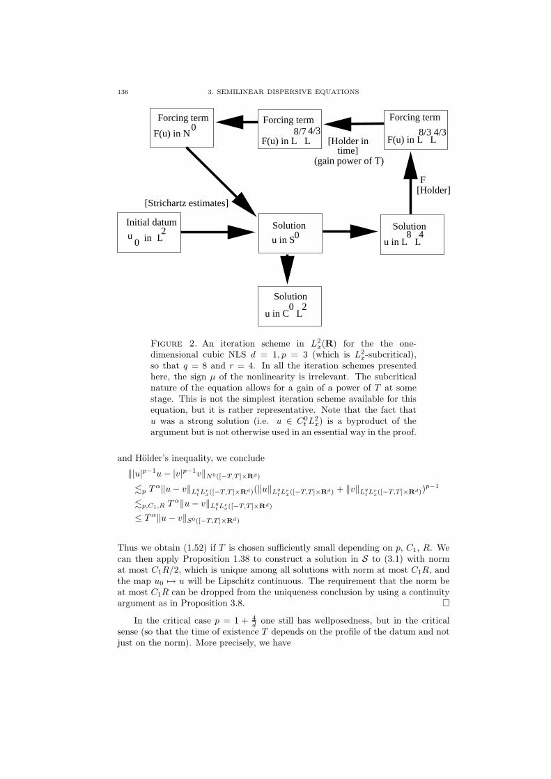
136 3. SEMILINEAR DISPERSIVE EQUATIONS
Forcing term
SolutionInitial datum
in0u L
2u in S0
Solution
u in C L0 2
Solution
u in L L8 4
F[Holder]
F(u) in L L
Forcing term
8/3 4/3F(u) in L L
8/74/3[Holder in
time]
Forcing term
F(u) in N0
(gain power of T)
[Strichartz estimates]
Figure 2. An iteration scheme in L2x(R) for the the one-
dimensional cubic NLS d = 1, p = 3 (which is L2x-subcritical),
so that q = 8 and r = 4. In all the iteration schemes presentedhere, the sign µ of the nonlinearity is irrelevant. The subcriticalnature of the equation allows for a gain of a power of T at somestage. This is not the simplest iteration scheme available for thisequation, but it is rather representative. Note that the fact thatu was a strong solution (i.e. u ∈ C0
t L2x) is a byproduct of the
argument but is not otherwise used in an essential way in the proof.
and Holder’s inequality, we conclude
‖|u|p−1u− |v|p−1v‖N0([−T,T ]×Rd)
.p Tα‖u− v‖Lq
tLrx([−T,T ]×Rd)(‖u‖Lq
tLrx([−T,T ]×Rd) + ‖v‖Lq
tLrx([−T,T ]×Rd))
p−1
.p,C1,R Tα‖u− v‖Lq
tLrx([−T,T ]×Rd)
≤ Tα‖u− v‖S0([−T,T ]×Rd)
Thus we obtain (1.52) if T is chosen sufficiently small depending on p, C1, R. Wecan then apply Proposition 1.38 to construct a solution in S to (3.1) with normat most C1R/2, which is unique among all solutions with norm at most C1R, andthe map u0 7→ u will be Lipschitz continuous. The requirement that the norm beat most C1R can be dropped from the uniqueness conclusion by using a continuityargument as in Proposition 3.8.
In the critical case p = 1 + 4d one still has wellposedness, but in the critical
sense (so that the time of existence T depends on the profile of the datum and notjust on the norm). More precisely, we have

3.3. LOCAL EXISTENCE THEORY 137
SolutionInitial datum
in0u L
2u in S0
Solution
u in C L0 2
Solution
u in L L4
F[Holder]
F(u) in L L
Forcing term
4/3
Forcing term
F(u) in N0
4
4/3
(large norm)
(large norm)
(small norm)
(small norm)(small norm)
(large norm)[Strichartz estimates]
Figure 3. An iteration scheme in L2x(R
2) for the two-dimensionalcubic NLS d = 2, p = 3 (which is L2
x-critical). For small data onecan simplify the scheme somewhat, but for large data it is impor-tant that the S0 is allowed to be large, while the L4
t,x component
of the S0 kept small; thus the main loop of the iteration shouldinvolve the L4
t,x norm more than once in order to close the argu-ment, because no gain of a power of T is available in the criticalsetting. This also makes the L4
t,x norm a controlling norm for theevolution.
Proposition 3.17 (Critical L2x NLS solutions). [Tsu] Let p be the L2
x-criticalexponent p = 1 + 4
d and let µ = ±1. Then the NLS (3.1) is locally wellposed
in L2x(R
d) in the critical sense. More specifically, given any R > 0 there existsε0 = ε0(R, d) > 0, such that whenever u∗ ∈ L2
x(Rd) has norm at most R, and I is
a time interval containing 0 such that
‖eit∆/2u∗‖L2(d+2)/dt,x (I×Rd)
≤ ε0
then for any u0 in the ball B := u0 ∈ L2x(R
d) : ‖u0 − u∗‖L2x(Rd) ≤ ε0 there exists
a unique strong L2x solution u ∈ S0(I × Rd) to (3.1), and furthermore the map
u0 7→ u is Lipschitz from B to S0(I × Rd) (of course, the Lipschitz constant willdepend on u∗).
This proposition is proven similarly to Proposition 3.15 and is left to Exercise3.18. Note that if the initial datum is sufficiently small in L2
x norm, then this Propo-sition, combined with Strichartz estimates, yields global existence in time. If theinitial datum is instead large, the Proposition combined with Strichartz estimates
138 3. SEMILINEAR DISPERSIVE EQUATIONS
will still give local existence, because the global L2(n+2)/nt,x norm of eit∆/2u∗ will be
finite, and hence can be localised to be small by choosing a sufficiently small timeinterval.
Remark 3.18. This proposition and the preceding one should be comparedagainst Principle 3.1. It turns out that the L2
x theory becomes bad for supercriticalpowers p > 1 + 4
d ; see Section 3.8 for further discussion and results.
Similar results hold for other regularities, such as H1x. Here it is convenient to
use the norms‖u‖S1(I×Rd) := ‖u‖S0(I×Rd) + ‖∇u‖S0(I×Rd)
and‖u‖N1(I×Rd) := ‖u‖N0(I×Rd) + ‖∇u‖N0(I×Rd)
Note that as the Schrodinger equation commutes with derivatives, we see from(3.26) that
(3.28) ‖u‖S1(I×Rd) .d ‖u(t0)‖H1x(I×Rd) + ‖F‖N1(I×Rd).
Let us give two sample results in dimension d = 3, in which theH1x-critical exponent
is the quintic one p = 5:
Proposition 3.19 (H1x(R
3) subcritical NLS solutions). Let µ = ±1. If 2 ≤p < 5, then the NLS (3.1) is locally wellposed in H1
x(R3) in the subcritical sense.
Remark 3.20. For this Proposition and the next, the reader may wish torefer back to the Strichartz “game board” for Schrodinger equations on H1
x(R3)
from Figure 1 of Chapter 2, and see how the various “moves” of Leibnitz, Holder,Sobolev, and Strichartz affect the “game pieces” u, ∇u, F (u), etc. on this board.(The objective of the iteration “game” is to construct a set of assumptions (thusplacing game pieces in various spaces with various norm bounds) on the solution,such that it is possible to apply a legal sequence of moves and end up with all thegame pieces returning to the same spaces but with better estimates.)
Proof. (Sketch) We apply Proposition 1.38 with S = S1([−T, T ]×R3), N =N1([−T, T ] × R3). By arguing as in Proposition 3.15, we will be done as soon aswe show that
‖|u|p−1u− |v|p−1v‖N1([−T,T ]×R3) .p,R Tα‖u− v‖S1
x([−T,T ]×R3)
for some α = α(p) > 0, whenever the S1x norms of u, v are O(R) for some R > 0.
Let us omit the domain [−T, T ]× R3 from the notation for brevity. Choosing theadmissible exponents (10, 30/13) for the S1
x norm and (2, 6) for the N1 norm, itsuffices to show that
‖∇k(|u|p−1u− |v|p−1v)‖L2
tL6/5x
.p,R Tα‖u− v‖
L10t W
1,30/13x
for k = 0, 1. Let us just deal with the higher order case k = 1, which is themore difficult of the two24. Observe that the gradient of |u|p−1u can be writtenas F1(u)∇u + F2(u)∇u, where F1, F2 : C → C are functions which grow likeFj(z) = Op(|z|p−1), and which have the Lipschitz-type bound ∇Fj(z) = Op(|z|p−2).
24A general principle in the local-in-time theory is that the highest order terms are alwaysthe most difficult to estimate, so that once those are dealt with the lower order terms should betreatable by a modification of the argument.
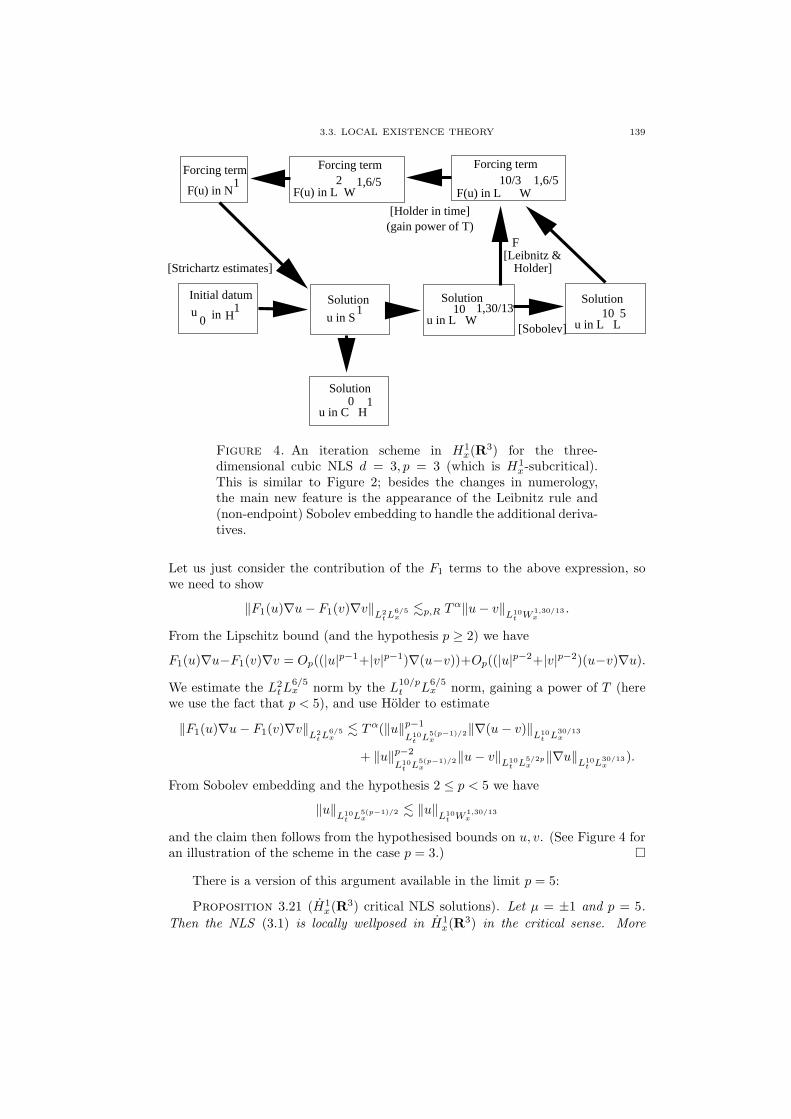
3.3. LOCAL EXISTENCE THEORY 139
Initial datum
in0u H
1Solution
u in S
Solution0
F
Forcing term
u in C H
Solution
u in L W10 1,30/13
Solution
u in L L[Sobolev]
[Leibnitz &Holder]
10
F(u) in L WF(u) in N1
Forcing term Forcing term2
F(u) in L W1,6/5
(gain power of T)[Holder in time]
5
10/3 1,6/5
1
1
[Strichartz estimates]
Figure 4. An iteration scheme in H1x(R
3) for the three-dimensional cubic NLS d = 3, p = 3 (which is H1
x-subcritical).This is similar to Figure 2; besides the changes in numerology,the main new feature is the appearance of the Leibnitz rule and(non-endpoint) Sobolev embedding to handle the additional deriva-tives.
Let us just consider the contribution of the F1 terms to the above expression, sowe need to show
‖F1(u)∇u− F1(v)∇v‖L2tL
6/5x
.p,R Tα‖u− v‖
L10t W
1,30/13x
.
From the Lipschitz bound (and the hypothesis p ≥ 2) we have
F1(u)∇u−F1(v)∇v = Op((|u|p−1+|v|p−1)∇(u−v))+Op((|u|p−2+|v|p−2)(u−v)∇u).
We estimate the L2tL
6/5x norm by the L
10/pt L
6/5x norm, gaining a power of T (here
we use the fact that p < 5), and use Holder to estimate
‖F1(u)∇u− F1(v)∇v‖L2tL
6/5x
. Tα(‖u‖p−1
L10t L
5(p−1)/2x
‖∇(u− v)‖L10
t L30/13x
+ ‖u‖p−2
L10t L
5(p−1)/2x
‖u− v‖L10
t L5/2px
‖∇u‖L10
t L30/13x
).
From Sobolev embedding and the hypothesis 2 ≤ p < 5 we have
‖u‖L10
t L5(p−1)/2x
. ‖u‖L10
t W1,30/13x
and the claim then follows from the hypothesised bounds on u, v. (See Figure 4 foran illustration of the scheme in the case p = 3.)
There is a version of this argument available in the limit p = 5:
Proposition 3.21 (H1x(R
3) critical NLS solutions). Let µ = ±1 and p = 5.
Then the NLS (3.1) is locally wellposed in H1x(R
3) in the critical sense. More

140 3. SEMILINEAR DISPERSIVE EQUATIONS
Initial datum
in0u H
1Solution
[Strichartz estimates]
u in S
Solution0
Forcing term
u in C H
Solution
u in L W10 1,30/13
Solution
u in L L[Sobolev]10
F(u) in L WF(u) in N1
Forcing term1,6/5
1
1. .
.
.
2.
10
(large norm)
(large norm) (large norm)
(large norm)
(small norm)
(small norm)(small norm)
.
F
[Leibnitz &Holder]
Figure 5. An iteration scheme in H1x for the three-dimensional
quintic NLS d = 3, p = 5 (which is H1x-critical). This rather tricky
scheme is similar to Figure 4 but with homogeneous norms, andwith certain norms identified as being small to compensate for thelack of a Holder in time (cf. Figure 3). It will be important thatthe smallness in L10
t,x is exploited more than once in order to closethe iteration properly.
precisely, given any R > 0 there exists ε0 = ε0(R) > 0, such that whenever u∗ ∈H1x(R
3) has norm at most R, and I is a time interval containing 0 such that
‖eit∆/2u∗‖L10t,x(I×R3) ≤ ε0
then for any u0 in the ball B := u0 ∈ H1x(R
3) : ‖u0 − u∗‖H1x(R3) ≤ ε0 there
exists a unique strong H1x solution u ∈ S1(I × R3) to (3.1), and furthermore the
map u0 7→ u is Lipschitz from B to S1(I × R3). Here ‖u‖S1 := ‖∇u‖S0 is thehomogeneous counterpart to the S1 norm.
We leave the proof of this to the exercises. Note that the L10t,x norm is controlled
(via Sobolev embedding) by the L10t W
1,30/13x norm, which in turn is controlled by
the S1 norm. From Strichartz estimates we thus conclude that
‖eit∆/2u∗‖L10t,x(R×R3) . ‖u∗‖H1
x(R3),
and thus Proposition 3.21 implies global wellposedness for quintic NLS on R3 withsmall energy, and local wellposedness (in the critical sense) for large energy. Again,this proposition and the preceding one should be compared against Principle 3.1.
In the supercritical case p > 5, the H1x perturbation theory breaks down com-
pletely; again, see Section 3.8. However in the defocusing case with 5 < p < 6 one

3.3. LOCAL EXISTENCE THEORY 141
can still construct global weak H1x solutions by a weak compactness method; see
Exercise 3.56.Similar wellposedness results exist for the NLW equation, and for the periodic
NLS equation; we leave this to the exercises. One can briefly summarise (andoversimplify) the known results for local wellposedness as follows. For NLS, onehas local wellposedness in Hs
x(Rd) as long as s ≥ 0 and the nonlinearity25 is Hs
x-subcritical or Hs
x-critical, though in the latter case the wellposedness is in thecritical sense (the time of existence depends on the profile of the datum rather thanthe norm, but for small norm one has global existence). See [CWeis2], [Caz2]. ForNLW, one has a similar result but with an additional constraint26 s ≥ sl, where sl is
the Lorentz regularity sl := d+14 − 1
p−1 ; this constraint is only relevant in the H1/2x -
subcritical cases p < 1 + 4d−1 ; see [LSog], [Sog]. For periodic NLS, the situation
is much less well understood, due to the lack of sharp Strichartz estimates in thissetting; see [Bou]. (The local theory for periodic NLW is essentially identical tonon-periodic NLW; see Exercise 3.24.)
Exercise 3.14 (Hk,k is a Banach algebra). Prove (3.24). (Hint: use the Leib-nitz rule, Holder, Sobolev, and Gagliardo-Nirenberg, controlling the lower orderterms before moving on to the higher ones. A Littlewood-Paley approach is possiblebut somewhat lengthy because of the need to continually commute the Littlewood-Paley operators with weights such as 〈x〉k.)
Exercise 3.15. Using the Fourier transform, show that the solution (3.15) tothe pseudoconformal focusing NLS blows up in Hs
x for any s > 0 as t → 0, butstays bounded in L2
x, and even goes to zero in Hsx for s < 0. (This reflects the fact
that this equation is locally wellposed in the subcritical sense in Hsx for s > 0, is
locally wellposed in the critical sense in L2x, and is illposed in Hs
x for s < 0.) Usingthis, show that when s < 0, one no longer has uniqueness for weak Hs
x solutions,and that Exercise 3.10 also breaks down for weak Hs
x solutions.
Exercise 3.16. Let u ∈ S1(I × R3) be an H1x-wellposed solution to quintic
NLS (so p = 5 and d = 3), and suppose that u(t0) ∈ Hk(R3) for some t0 ∈ I andsome integer k ≥ 0. Show that u(t) ∈ Hk(R3) for all t ∈ I, and in fact
‖u(t0)‖Hk(R3) .‖u‖S1(I×R3)‖u(t0)‖Hk(R3).
(Hint: Let M := ‖u‖S1(I×R3). Subdivide I into time intervals Ij where the L10t,x
norm on Ij is small compared withM . Then use Strichartz estimates and continuityarguments to establish Sk control on each Ij .)
Exercise 3.17 (Unconditional uniqueness). Let u, v ∈ C0t H
1x(I×R3) be strong
H1x solutions to quintic NLS (so p = 5 and d = 3) with u(t0) = v(t0) for some
t0 ∈ I. Show that u = v. (Hint: Let J be a small time interval containing t0,and use Strichartz estimates to control ‖u − v‖L2
tL6x(J×R3) in terms of itself and
‖u − v‖L∞t L6
x(J×R3). Then use the continuity of u − v in H1x and hence in L6
x toclose the argument. To extend from J back to I, use the continuity method.) Inparticular, this shows that the H1
x-wellposed solution given by Proposition 3.21 is
25There is also a technical smoothness condition required on the nonlinearity in the non-algebraic case; see [CWeis2], [Caz2].
26Again, we need a smoothness condition on the nonlinearity. Also this result is not fullyestablished in high dimension n ≥ 4 when s is very close to zero, for technical reasons; see [Tao].
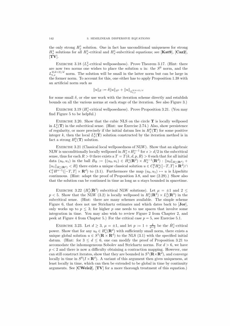
142 3. SEMILINEAR DISPERSIVE EQUATIONS
the only strong H1x solution. One in fact has unconditional uniqueness for strong
H1x solutions for all H1
x-critical and H1x-subcritical equations; see [Kat9], [Caz2],
[TV].
Exercise 3.18 (L2x-critical wellposedness). Prove Theorem 3.17. (Hint: there
are now two norms one wishes to place the solution u in: the S0 norm, and the
L2(d+2)/dt,x norm. The solution will be small in the latter norm but can be large in
the former norm. To account for this, one either has to apply Proposition 1.38 withan artificial norm such as
‖u‖S := δ‖u‖S0 + ‖u‖L
2(d+2)/dt,x
for some small δ, or else use work with the iteration scheme directly and establishbounds on all the various norms at each stage of the iteration. See also Figure 3.)
Exercise 3.19 (H1x-critical wellposedness). Prove Proposition 3.21. (You may
find Figure 5 to be helpful.)
Exercise 3.20. Show that the cubic NLS on the circle T is locally wellposedin L2
x(T) in the subcritical sense. (Hint: use Exercise 2.74.) Also, show persistenceof regularity, or more precisely if the initial datum lies in Hk
x (T) for some positiveinteger k, then the local L2
x(T) solution constructed by the iteration method is infact a strong Hk
x (T) solution.
Exercise 3.21 (Classical local wellposedness of NLW). Show that an algebraicNLW is unconditionally locally wellposed inHs
x×Hs−1x for s > d/2 in the subcritical
sense, thus for eachR > 0 there exists a T = T (k, d, p, R) > 0 such that for all initialdata (u0, u1) in the ball BR := (u0, u1) ∈ Hs
x(Rd) × Hs−1
x (Rd) : ‖u0‖Hsx(Rd) +
‖u1‖Hsx(Rd) < R there exists a unique classical solution u ∈ C0
tHsx([−T, T ]×Rd)∩
C1tH
s−1([−T, T ] × Rd) to (3.1). Furthermore the map (u0, u1) 7→ u is Lipschitzcontinuous. (Hint: adapt the proof of Proposition 3.8, and use (2.29).) Show alsothat the solution can be continued in time as long as u stays bounded in spacetime.
Exercise 3.22 (H1x(R
3) subcritical NLW solutions). Let µ = ±1 and 2 ≤p < 5. Show that the NLW (3.2) is locally wellposed in H1
x(R3) × L2
x(R3) in the
subcritical sense. (Hint: there are many schemes available. The simple schemeFigure 6, that does not use Strichartz estimates and which dates back to [Jor],only works up to p ≤ 3; for higher p one needs to use spaces that involve someintegration in time. You may also wish to review Figure 2 from Chapter 2, andpeek at Figure 4 from Chapter 5.) For the critical case p = 5, see Exercise 5.1.
Exercise 3.23. Let d ≥ 3, µ = ±1, and let p := 1 + 4d−2 be the H1
x-critical
power. Show that for any u0 ∈ H1x(R
d) with sufficiently small norm, there exists aunique global solution u ∈ S1(R × Rd) to the NLS (3.1) with the specified initialdatum. (Hint: for 3 ≤ d ≤ 6, one can modify the proof of Proposition 3.21 toaccomodate the inhomogeneous Sobolev and Strichartz norms. For d > 6, we havep < 2 and there is now a difficulty obtaining a contraction mapping. However, onecan still construct iterates, show that they are bounded in S1(R×Rd), and convergelocally in time in S0(I ×Rd). A variant of this argument then gives uniqueness, atleast locally in time, which can then be extended to be global in time by continuityarguments. See [CWeis2], [TV] for a more thorough treatment of this equation.)

3.4. CONSERVATION LAWS AND GLOBAL EXISTENCE 143
Solution
Forcing term
(gain power of T)[Holder in time]
0
F(u) in L L1 2
F
Forcing term
Solution
u in C L0 6
F(u) in C L0 2
[energy estimates][Holder]
[Sobolev]u in L 1
2 u in C L
1
u0in H1
2u in C H1
Initial data
Figure 6. A simple iteration scheme in H1x × L2
x, based on theenergy estimate, for the three-dimensional cubic NLW d = 3, p = 3.For higher powers p, Strichartz estimates and spaces are needed.
Exercise 3.24. Suppose that an NLW on Rd is known to be locally wellposedin Hs
x×Hs−1x in the subcritical sense for some s ≥ 0. Assume also that one has the
finite speed of propagation result, Proposition 3.3, for Hsx ×Hs−1
x -wellposed solu-tions. (In practice, this hypothesis can either be deduced from the correspondingresult for classical solutions by a limiting argument, or else by direct inspection ofthe iterates used to construct the wellposed solution.) Show that the correspondingperiodic NLW on Td is also locally wellposed in Hs
x ×Hs−1x . (You may find Exer-
cise A.18 to be useful.) This type of descent argument does not always work in thenonperiodic setting, especially for large times; indeed, it is quite possible for thebehaviour of an equation for large, localized data to be better in higher dimensionsthan in lower ones, due to the increased dispersion available.
Exercise 3.25 (Analytic wellposedness). Consider an algebraic NLS, and lets > d/2 and R > 0. By the Hs
x version of Proposition 3.8, we know that thereexists T = Td,p,s > 0 such that every u0 ∈ Hs
x(Rd) with norm at most R extends
to a strong Hsx solution u ∈ C0
tHsx([0, T ]×Rd). Show that if T is small enough, the
map u0 7→ u is in fact an real analytic map, thus there is a power series expansionu =
∑∞k=0 Nk(u0, . . . , u0) which converges absolutely in C0
tHsx([0, T ] × Rd), where
for each k, Nk is a k-multilinear operator fromHsx(R
d) to C0tH
sx([0, T ]×Rd). (Hint:
you can adapt the proof of the Cauchy-Kowalevski theorem, see Exercise 1.1.) Oneconsequence of analyticity is that the solution map is also infinitely differentiablefrom Hs
x to C0tH
sx.
3.4. Conservation laws and global existence
The journey of a thousand miles begins with one step. (Lao Tzu)
The wellposedness theory of the previous section allowed us to use iterativemethods to construct local-in-time solutions to NLS and NLW given suitable reg-ularity assumptions on the initial data; if the datum was also small in a critical
144 3. SEMILINEAR DISPERSIVE EQUATIONS
norm (e.g. small in L2x norm for the L2
x-critical NLS, or small in H1x norm for the
H1x-critical NLS) then one obtained a global solution also. These methods were
perturbative in nature (using the Duhamel formula to approximate the nonlinearevolution by the linear evolution) and thus do not work directly for large data andlong times (since one expects the evolution to be genuinely nonlinear in this case).However, in these cases one can use non-perturbative tools to gain enough controlon the equation to prevent the solution from blowing up. In this section we describethe most important tool for doing this, namely the conservation laws.
As before, we begin by discussing the nonlinear Schrodinger equation (3.1). Inthis case we have two independent conservation laws, namely energy conservationand mass/momentum conservation27. The latter can be most effectively describedby pseudo-stress-energy tensor Tαβ , defined for α, β = 0, 1, . . . , d by by
T00 = |u|2
T0j = Tj0 = Im(u∂xju)
Tjk = Re(∂xju∂xku) − 1
4δjk∆(|u|2) +
(p− 1)µ
p+ 1δjk|u|p+1.
If the solution is sufficiently smooth, one easily verifies the local conservation laws(2.35); see Exercise 3.26. In particular, for smooth decaying solutions, this leads toconservation of total mass M [u(t)], defined by
(3.29) M [u(t)] :=
∫
Rd
T00(t, x) dx =
∫
Rd
|u(t, x)|2 dx
and total momentum ~p[u(t)] = (p1[u(t)], . . . , pd[u(t)]), defined by
pj [u(t)] :=
∫
Rd
T0j(t, x) dx =
∫
Rd
Im(u∂xju) dx;
again, see Exercise 3.26. As in Section 2.4, the pseudo-stress-energy tensor alsoyields many other important conservation laws and montonicity formulae; we willdevelop some of these later in this chapter.
The above conservation laws are initially only justified for smooth decayingsolutions. However, if the conservation law is controlled by an Hs
x norm, and onehas a satisfactory wellposedness theory at Hs
x, then there is a standard limitingargument that allows one to extend these conservation laws to these Hs
x-well posedsolutions. We illustrate this principle with the example of the one-dimensionalcubic NLS:
Proposition 3.22 (Conservation law for a wellposed solution). Let d = 1,p = 3, µ = ±1. Let u ∈ S0(I × Rd) ⊆ C0
t L2x(I × Rd) be a strong solution to (3.1)
defined on some time interval I. Let the total mass M [u(t)] be defined by (3.29).Then M [u(t)] = M [u(t0)] for all t0, t ∈ I.
Proof. Since I is the increasing union of open intervals we may assume with-out loss of generality that I is open. Fix t0 ∈ I. Since u ∈ C0
t L2x(I × R), the set
of times t ∈ I : M [u(t)] = M [u(t0)] is closed in I, and it clearly contains t0, so itsuffices by the continuity method to show that this set is open. In other words, it
27In the special case of the one-dimensional cubic NLS (d = 1, p = 3), it turns out thatthe equation is completely integrable and there are in fact infinitely many conservation laws, seeExercise 3.36.

3.4. CONSERVATION LAWS AND GLOBAL EXISTENCE 145
suffices to show that for any t1 ∈ I, that we have M [u(t)] = M [u(t1)] for all timest in a neighbourhood of t1.
By time translation invariance we can take t1 = 0. Set u0 := u(0). We
can approximate u0 as the limit in L2x(R
d) of a sequence u(n)0 ∈ H100
x (Rd) (say)of smooth initial data, which will be uniformly bounded in L2
x(Rd). Applying
Proposition 3.15, we can obtain a time interval [−T, T ] ⊂ I independent of n, and
strong solutions u(n) ∈ S0([−T, T ] × Rd) to (3.1) with initial data u(n)(0) = u(n)0 .
Since u(n)0 converges to u0 in L2
x, the uniqueness and continuity conclusions of
Proposition 3.15 guarantee that u(n) will converge to u in S0([−T, T ]×Rd). Next,since the u(n) are uniformly bounded in S0([−T, T ]×Rd), they are also uniformlybounded in L4
tL∞x ([−T, T ]×Rd) and hence in L2
tL∞x ([−T, T ]×Rd). We may thus
apply Proposition 3.11 (and the remarks following that proposition) and concludethat u(n) ∈ C0
tHsx([−T, T ] × Rd) for any s > d/2. From this, Sobolev embedding,
and the equation (3.1) it is easy to see that u(n) is smooth on [−T, T ]× Rd. Thisis enough regularity for us to apply the classical mass conservation law in Exercise3.26 and conclude that
∫
Rd
|u(n)(t, x)|2 dx =
∫
Rd
|u(n)(0, x)|2 dx
for all t ∈ [−T, T ]. Since u(n) converges to u in S0([−T, T ]×Rd), it also convergesin C0
t L2x([−T, T ]× Rd), and hence on taking limits as n→ ∞ we have
∫
Rd
|u(t, x)|2 dx =
∫
Rd
|u(0, x)|2 dx
and hence M [u(t)] = M [u(0)] for all t in a neighbourhood of t, as desired.
Note that the full power of the wellposedness theory was used here; not only theexistence aspect of the theory, but also the uniqueness, persistence of regularity, andcontinuous dependence on the data. This basic argument - obtaining conservationlaws for rough solutions by approximating them by smooth solutions - is quitegeneral and extends to many other equations. There is an additional twist howeverin the case when the nonlinearity is not algebraic (i.e. p is not an odd integer),because it is often not possible in such cases to obtain an approximating solutionthat is sufficiently smooth that one can justify the conservation law classically. Insuch cases one must not only regularise the initial data, but also regularise theequation as well; this requires a further aspect of the wellposedness theory, namelythe stability theory of the equation, which we will address in Section 3.7.
A conservation law can often, but not always, be combined with a local well-posedness result to obtain a global wellposedness result. Let us illustrate this witha simple example:
Proposition 3.23. [Tsu] Let d = 1, p = 3, µ = ±1, and t0 ∈ R. Letu0 ∈ L2
x(Rd), and let I be any bounded time interval containing t0. Then there is
a unique strong solution u ∈ S0(I ×Rd) ⊆ C0t L
2x(I ×Rd) to (3.1) defined on some
time interval I. Furthermore, the map u0 7→ u is a continuous map from L2x to
S0(I × Rd).
In particular, this proposition gives a global strong solution u ∈ C0t L
2x(R×Rd)
to (3.1). However this solution is only in the S0 space locally in time. (Indeed, in

146 3. SEMILINEAR DISPERSIVE EQUATIONS
the focusing case µ = −1, soliton solutions to this equation exist which do not lieglobally in S0.)
Proof. we first use time translation invariance and time reversal symmetryto reduce to the case when t0 = 0 and I = [0, T ] for some T > 0. (Note that byExercise 3.11 one can easily glue a strong solution on an interval such as [0, T ] toa strong solution to an interval such as [−T, 0], and stay in S0.)
We give two proofs of this result; they are equivalent, but offer slightly differentperspectives as to how a conservation law extends a local existence result to a globalexistence result. For the first proof, we divide the long time interval [0, T ] intoshorter time steps, where on each smaller interval the perturbative theory gives alocal solution. More precisely, let M [u(0)] := ‖u0‖2
L2x(Rd) denote the initial mass,
and observe from Proposition 3.15 that there exists a time τ = τ(M [u(0)]) > 0such that the equation (3.1) will have a local strong solution in S0([t0, t0 + τ ]×Rd)whenever the initial datum u(t0) has mass less than or equal to M [u(0)]. We nowsplit the time interval [0, T ] as a finite union of intervals [tn, tn+1], where eachinterval has length less than or equal to τ , and t0 = 0. By applying Proposition3.15 followed by Proposition 3.23 (and Exercise 3.11), an easy induction showsthat for every n we can construct a strong solution u to (3.1) in S0([0, tn] × Rd),and thus we eventually obtain a strong solution to S0([0, T ] × Rd); see Figure 7.Uniqueness follows from Proposition 3.15 and a continuity argument similar to thatused to prove Exercise 3.13. The continuous dependence follows by concatenatingthe continuous dependence results on each of the intervals [tn, tn+1], using the factthat the S0([tn, tn+1] × Rd) norm of u controls the L2
x norm of u(tn+1), and usingthe fact that the composition of continuous maps is continuous.
The second proof proceeds by contradiction; it is quicker but is more indirect(and does not give the continuous dependence as easily). We sketch it as follows.Just as the Picard existence and uniqueness theorems imply a blowup criterion forODE (Proposition 1.17), the existence and uniqueness theory in Proposition 3.15gives a blowup criterion for L2
x strong solutions to (3.1), namely that these solutionswill exist globally unless the L2
x norm goes to infinity in finite time. However, Propo-sition 3.22 clearly implies that the L2
x norm of a strong solution stays bounded.Thus blowup cannot occur, and one must instead have global existence.
One can combine this global existence result with persistence of regularity the-ory (e.g. Proposition 3.11) to show that the global solution constructed in Propo-sition 3.23 preserves regularity; see Exercise 3.28. In particular, with a smoothdecaying initial datum we have a global smooth solution to the one-dimensionalcubic NLS.
Similar arguments give global L2x-wellposedness for any L2
x-subcritical equation.The situation is remarkably different when one considers the two-dimensional cubicNLS (d = 2, p = 3, µ = ±1). The key difference is that whereas the one-dimensionalcubic NLS was L2
x-subcritical, the two-dimensional cubic NLS is L2x-critical. This
is reflected in the local wellposedness theory for this equation, given by Proposition3.17. If the initial datum has a sufficiently small L2
x norm, then this propositionalready gives a global existence result without any need for a conseration law. How-ever, when the L2
x norm is large, one cannot simply combine the conservation lawwith the local existence theory to obtain a global existence theory; the problem isthat the time of existence given by the local wellposedness theory does not depend
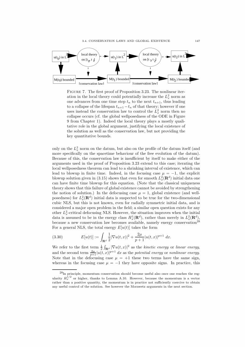
3.4. CONSERVATION LAWS AND GLOBAL EXISTENCE 147
on [t , t ]
local theory u(t ) in L2
on [t , t ]
local theory
M(t ) boundedM(t ) bounded
u(t ) in L2
M(t ) bounded
u(t ) in L2
22
20
00 1
1
1
1
[conservation law] [conservation law]
Figure 7. The first proof of Proposition 3.23. The nonlinear iter-ation in the local theory could potentially increase the L2
x norm asone advances from one time step tn to the next tn+1, thus leadingto a collapse of the lifespan tn+1− tn of that theory; however if oneuses instead the conservation law to control the L2
x norm then nocollapse occurs (cf. the global wellposedness of the ODE in Figure9 from Chapter 1). Indeed the local theory plays a mostly quali-tative role in the global argument, justifying the local existence ofthe solution as well as the conservation law, but not providing thekey quantitative bounds.
only on the L2x norm on the datum, but also on the profile of the datum itself (and
more specifically on the spacetime behaviour of the free evolution of the datum).Because of this, the conservation law is insufficient by itself to make either of thearguments used in the proof of Proposition 3.23 extend to this case; iterating thelocal wellposedness theorem can lead to a shrinking interval of existence, which canlead to blowup in finite time. Indeed, in the focusing case µ = −1, the explicitblowup solution given in (3.15) shows that even for smooth L2
x(Rd) initial data one
can have finite time blowup for this equation. (Note that the classical uniquenesstheory shows that this failure of global existence cannot be avoided by strengtheningthe notion of solution.) In the defocusing case µ = 1, global existence (and well-posedness) for L2
x(Rd) initial data is suspected to be true for the two-dimensional
cubic NLS, but this is not known, even for radially symmetric initial data, and isconsidered a major open problem in the field; a similar open question exists for anyother L2
x-critical defocusing NLS. However, the situation improves when the initialdata is assumed to be in the energy class H1
x(Rd), rather than merely in L2
x(Rd),
because a new conservation law becomes available, namely energy conservation28
For a general NLS, the total energy E[u(t)] takes the form
(3.30) E[u(t)] :=
∫
Rd
1
2|∇u(t, x)|2 +
2µ
p+ 1|u(t, x)|p+1 dx.
We refer to the first term 12
∫Rd |∇u(t, x)|2 as the kinetic energy or linear energy,
and the second term 2µp+1 |u(t, x)|p+1 dx as the potential energy or nonlinear energy.
Note that in the defocusing case µ = +1 these two terms have the same sign,whereas in the focusing case µ = −1 they have opposite signs. In practice, this
28In principle, momentum conservation should become useful also once one reaches the reg-
ularity H1/2x or higher, thanks to Lemma A.10. However, because the momentum is a vector
rather than a positive quantity, the momentum is in practice not sufficiently coercive to obtainany useful control of the solution. See however the Morawetz arguments in the next section.
148 3. SEMILINEAR DISPERSIVE EQUATIONS
means that the energy conservation law is more coercive (gives more control on thesolution) in the defocusing case than in the focusing case.
The following heuristic principle, related to Principle 1.37 and Principle 3.1,can be helpful in predicting behaviour of equations in the energy class:
Principle 3.24 (Energy principle). Suppose a solution has finite energy. Ifthe linear energy dominates the nonlinear energy, we expect linear behaviour; if thenonlinear energy dominates the linear energy, we expect nonlinear behaviour.
This heuristic has very little rigorous justification to back it up, yet is surpris-ingly accurate in many cases, as we shall see in several places in this text.
For sufficiently classical solutions one can justify conservation of energy E[u(t)]by integration by parts; see Exercise 3.31. In the energy subcritical cases sc ≤ 1, theenergy functional u 7→ E[u] is continuous in H1
x(Rd) (Exercise 3.32). Combining
this with the local H1x wellposedness theory (such as Proposition 3.19 and 3.21) as
in Proposition 3.22, one can extend the energy conservation law to all H1x-critical
and H1x-subcritical wellposed solutions. (In fact one has this for strong solutions
also, thanks to uniqueness results such as Exercise 3.17. The high-dimensional casesn > 6 are a little tricky; see [Caz2], [TV].)
Let us now return to the two-dimensional cubic NLS (d = 2, p = 3), and seewhat this new conservation law gives us. The focusing and defocusing cases arenow rather different (as one can already see from the blowup solution (3.15)). Inthe defocusing case, it is clear that energy and mass together will control the H1
x
norm of the solution:‖u(t)‖2
H1x
. E[u(t)] +M [u(t)].
Conversely, the Gagliardo-Nirenberg inequality (Proposition A.3) shows that theenergy and mass are controlled by the H1
x norm:
E[u(t)] . ‖u(t)‖2H1
x(1 + ‖u(t)‖2
L2x) . ‖u(t)‖2
H1x(1 + ‖u(t)‖2
H1x)
M [u(t)] = ‖u(t)‖2L2
x. ‖u(t)‖2
H1x.
From these bounds and the energy and mass conservation laws we see that forany H1
x-wellposed solution, the H1x norm of the solution u(t) at some later time
t is bounded by a quantity depending only on the H1x norm of the initial datum.
On the other hand, Proposition 3.19 shows that an H1x wellposed solution can be
continued in time as long as the H1x norm does not go to infinity. Combining these
two statements we obtain
Proposition 3.25. The defocusing two-dimensional cubic NLS (d = 2, p =3, µ = +1) is globally wellposed in H1
x. Indeed for any u0 ∈ H1x and any time
interval I containing t0, the Cauchy problem (3.1) has an H1x-wellposed solution
u ∈ S1(I × R2) ⊆ C0tH
1x(I × R2).
The reader should see how the scheme in Figure 7 is modified to accomodatethe utilisation of two conservation laws (mass and energy) rather than just one.
Remark 3.26. This argument is in fact quite general and works for any H1x-
subcritical defocusing NLS; see for instance [Caz2] or Exercise 3.35. One also hasglobal wellposedness in H1
x for the H1x-critical equation but this is significantly more
difficult and will be discussed in Chapter 5. This fits well with Principle 3.24, sincein the H1
x-critical equation, Sobolev embedding only barely manages to control thenonlinear energy in terms of the linear energy.
3.4. CONSERVATION LAWS AND GLOBAL EXISTENCE 149
Remark 3.27. In the focusing case, a problem arises because of the negativesign of the nonlinear component of the energy E[u(t)]. This means that while theenergy is still controlled by the H1
x norm, the H1x norm is not necessarily controlled
by the energy. Indeed, (3.15) shows that global wellposedness fails for some H1x
data. However this turns out to be the borderline case: for any H1x data with mass
strictly less than that of the blowup solution in (3.15), the Gagliardo-Nirenberginequality becomes strong enough again to control the H1
x norm by the energy andthus regain global wellposedness. See Exercise 3.33.
The above discussion was for the two-dimensional cubic NLS, which was L2x-
critical. For equations which are L2x-subcritical, it turns out that the Gagliardo-
Nirenberg inequality is now so strong that the sign µ of the nonlinearity playsessentially no role in the global theory; see Exercise 3.34. For equations which areL2x-supercritical but H1
x-subcritical or H1x-critical, the defocusing equation enjoys
global existence in H1x as discussed above, but blowup can occur for the focusing
equation unless a suitable smallness condition is met; see Exercise 3.35 and Section3.8.
Having discussed the conservation laws for the NLS, we now turn to the NLW(3.2), which we write using the Minkowski metric as
(3.31) ∂α∂αu = µ|u|p−1u.
For this equation there is no mass conservation law, and the energy/momentumconservation laws can be unified via the stress-energy tensor
(3.32) Tαβ := Re(∂αu∂βu) − 1
2gαβRe(∂γu∂γu+
2µ
p+ 1|u|p+1)
(compare with (2.45)). In coordinates,
T00 = T00 =1
2|∂tu|2 +
1
2|∇u|2 +
µ
p+ 1|u|p+1
T0j = −Tj0 = −Re(∂tu∂xju)
Tjk = Tjk = Re(∂xju∂xku) − δjk
2(|∇u|2 − |∂tu|2 +
2µ
p+ 1|u|p+1).
From (3.31) we easily verify the divergence-free property
(3.33) ∂αTαβ = 0
or in coordinates
(3.34) ∂tT00 + ∂xj T
0j = 0; ∂tT0j + ∂xk
Tjk = 0,
for classical solutions at least. This leads (for classical, decaying solutions) toconservation of the total energy
(3.35) E[u[t]] :=
∫
Rd
T00(t, x) dx =
∫
Rd
1
2|∂tu|2 +
1
2|∇u|2 +
µ
p+ 1|u|p+1 dx

150 3. SEMILINEAR DISPERSIVE EQUATIONS
and total momentum29
pj(u[t]) :=
∫
Rd
T0j(t, x) dx = −∫
Rd
Re(∂tu∂xju) dx.
By the limiting arguments as before, these conservation laws can be extended toH1x-wellposed solutions, as long as the equation is either H1
x-subcritical or H1x-
critical.For defocusing H1
x-subcritical equations, the energy conservation can lead toglobal existence in even for large initial data. Let us illustrate this with the three-dimensional cubic NLW (d = 3, p = 3, µ = +1). From Exercise 3.22 we have a localwellposedness result for initial data in H1
x×L2x in the subcritical sense, which easily
implies a blowup criterion, namely that the H1x × L2
x wellposed solutions to thisequation can be continued in time as long as the quantity ‖u(t)‖H1
x+ ‖∂tu(t)‖L2
x
does not go to infinity in finite time. To bound this quantity, we observe from(3.35) and energy conservation that we can bound the homogeneous component ofthis quantity easily:
‖u(t)‖H1x
+ ‖∂tu(t)‖L2x
. E[u[t]]1/2 = E[u[0]]1/2.
To control the lower order term ‖u(t)‖L2x
we use the fundamental theorem of cal-culus and Minkowski’s inequality:
‖u(t)‖L2x≤ ‖u(0)‖L2
x+ |
∫ t
0
‖∂tu(s)‖L2xds|
. ‖u(0)‖L2x
+ |∫ t
0
E[u[s]]1/2 ds|
= ‖u(0)‖L2x
+ |t|E[u[0]]1/2.
Thus we can control the H1x × L2
x norm of u[t] by a quantity that depends mostlyon the initial data:
‖u(t)‖H1x
+ ‖∂tu(t)‖L2x
. ‖u(0)‖L2x
+ (1 + |t|)E[u[0]]1/2.
In particular, if u[0] ∈ H1x × L2
x, then E[u[0]] is finite and the quantity ‖u(t)‖H1x
+
‖∂tu(t)‖L2x
cannot go to infinity in finite time for any H1x × L2
x-wellposed solution.
Comparing this with the blowup criterion30 we see that we have a global C0tH
1x ∩
C1t L
2x strong solution to this equation for any initial data in the energy space
H1x × L2
x. Once one has this global existence result in the energy class, we alsoobtain it for smoother classes; see Exercise 3.38.
The above argument in fact works for any H1x-subcritical NLW; see [GV2],
[Sog]. The case of the H1x-critical equation is again more delicate (because the
lifespan given by the local existence theorem depends on the profile of the data as
29Note the presence of the time derivative, which is absent for the NLS momentum. Indeed,
while the NLS momentum is naturally associated to the regularity H1/2x , the NLW momentum is
associated to the regularity H1x, and thus is of the same order as the energy. Thus the relationship
between momentum and energy in NLW is different from that in NLS, which turns out to be acrucial difference in the critical scattering theory, see Chapter 5 below.
30It is instructive to use the other approach to global existence from Proposition 3.23, namelydividing up a long time interval into short ones. Here, because the quantity ‖u(t)‖H1
x+‖∂tu(t)‖L2
x
could grow linearly in t, the interval of existence guaranteed by the local theory could decaypolynomially in t. However, the length of this interval will not go to zero in finite time, which isall one needs to establish global existence.

3.4. CONSERVATION LAWS AND GLOBAL EXISTENCE 151
well as on the H1×L2x norm, and so the blowup criterion is more subtle), and will be
treated in Section 5.1; again, this is in accordance with Principle 3.24. For focusingNLW, there are no Gagliardo-Nirenberg tricks available to control the nonlinearity(since there is no mass conservation law), and indeed for such equations large datacan lead to blowup no matter what the power is; see Exercise 3.9.
Exercise 3.26. Verify (2.35) for the pseudo-stress-energy tensor for C3t,x,loc
solutions to (3.1). These conservation laws may seem somewhat miraculous, butcan be explained using Lagrangian methods; see [SSul], as well as Exercises 3.30,3.40. Conclude that if u ∈ C3
t,x,loc(I × Rd) is a solution to (3.1) which also lies in
C0tH
sx(I ×Rd) for a sufficiently large s, then we have mass conservation M [u(t)] =
M [u(t0)] and momentum conservation pj(t) = pj(t0) for all t, t0 ∈ I. (In order tojustify the integration by parts, one needs to apply a smooth cutoff in space, andthen let the cutoff go to infinity, using the Hs
x control on u to show that the errorincurred by the cutoff goes to zero.) These rather restrictive regularity conditionscan usually be removed by a limiting argument.
Exercise 3.27. Obtain the analogue of Proposition 3.22 but with d = 2 insteadof d = 1. (The challenge here is that the equation is now L2
x-critical instead of L2x-
subcritical, and one has to use Proposition 3.17 instead of Proposition 3.15.)
Exercise 3.28. Let p = 3, d = 1, µ = ±1, and let u0 ∈ Hsx(R) for some s ≥ 0.
Show that the solution u constructed in Proposition 3.23 is a strong Hsx solution,
and we have the bound ‖u(t)‖Hsx
. exp(Ct)‖u0‖Hsx, where C = C(s, ‖u0‖L2
x) > 0
depends only on s and the initial mass.
Exercise 3.29. Show that the energy (3.30) is formally the Hamiltonian forthe NLS (3.1) using the symplectic structure from Exercise 2.47. Also use Noether’stheorem to formally connect the mass conservation law to the phase invariance ofNLS, and the momentum conservation law to the translation invariance of NLS.
Exercise 3.30. Use Exercise 3.2 to link the pseudo-stress-energy tensor andenergy conservation law for d-dimensional NLS to the stress-energy tensor for d+1-dimensional NLW. (In d+ 1 dimensions, you may find it convenient to introduce anull frame (t′, x′, x1, . . . , xd) where t′ := t− xd+1 and x′ := t+ xd+1, and computethe coordinates of the stress-energy tensor in that frame.)
Exercise 3.31. Let u ∈ C3t,x(I × Rd) be a classical solution to (3.1). Verify
the identity
∂t(1
2|∇u(t, x)|2 +
2µ
p+ 1|u(t, x)|p+1) =
∂j(1
2Im(∂jku(t, x)∂ku(t, x)) + µ|u(t, x)|p−1Im(u(t, x)∂ju(t, x))).
If u is also in C0tH
k,kx (I × Rd) for some sufficiently large k, deduce the energy
conservation law E[u(t1)] = E[u(t0)] for all t0, t1 ∈ I (by arguing as in Exercise3.26).
Exercise 3.32. If sc ≤ 1, show that the energy functional u 7→ E[u] is well-defined and continuous on the space H1
x(Rd). (Hint: use Sobolev embedding and
an estimate similar to (3.27).) When sc > 1, show that the energy is not alwaysfinite for H1
x(Rd) data.
152 3. SEMILINEAR DISPERSIVE EQUATIONS
Exercise 3.33. [Wei] Let u0 ∈ H1x(R
2) have mass strictly less than the massof the blowup solution in (3.15). Show that there is a global strong H1
x solution tothe cubic defocusing two-dimensional NLS (i.e. (3.1) with d = 2, p = 3, µ = −1)with initial datum u0. (Hint: you will need the relationship between Q and Wmax
given by Lemma B.1 in order to control the H1x norm by the energy.) Note that
this is consistent with Principle 3.24. There has been much recent analysis of thecase when the mass is exactly equal to, or slightly higher than, the mass of theblowup solution (3.15): see [Mer2], [Mer3], [MR], [MR2], [MR3].
Exercise 3.34. Let u be an H1x-wellposed solution to the one-dimensional
cubic NLS (d = 1, p = 3, µ = ±1) with initial datum u0; this is a global so-lution by Proposition 3.23 and persistence of regularity. Establish the bound‖u(t)‖H1
x(R) .‖u0‖H1x(R) 1 for all times t, regardless of whether the equation is
focusing or defocusing. (The point here is that in the L2x-subcritical equations, the
Gagliardo-Nirenberg inequality allows one to control the nonlinear component ofthe energy by a fractional power of the linear component of the energy, times afactor depending only on the conserved mass; cf. Exercise 1.22 and Principle 3.24.)
Exercise 3.35. Consider the defocusing three-dimensional cubic NLS (d =3, p = 3). Show that one has global H1
x-wellposed solutions if the initial datumu0 is sufficiently small in H1
x(R3) norm, and in the defocusing case one has global
H1x-wellposedness for arbitrarily large H1
x(R3) initial data. (Again, one can rely
primarily on the Gagliardo-Nirenberg inequality and the conservation laws. Analternate approach is to develop a small data global existence theory at the crit-
ical regularity H1/2x (R3) by perturbative arguments, and then use persistence of
regularity to move from H1/2x to H1
x.)
Exercise 3.36. Consider the one-dimensional cubic NLS (d = 1, p = 3). Itturns out that there is a conserved quantity (at least for classical solutions to NLS)of the form
E2(u) :=
∫
R
|∂xxu|2 + c1µ|∂xu|2|u|2 + c2µRe((u∂xu)2)) + c3µ
2|u|6 dx
for certain absolute constants c1, c2, c3 whose exact value is unimportant here. (Theverification of this conservation law is extremely tedious if done directly, thoughthe machinery in Section 4.2 can expedite some of the algebra; one can also proceedvia the Lax pair formulation of this equation.) Assuming this, conclude the bound‖u(t)‖H2
x(R) .‖u0‖H2x(R) 1 for all times t, at least for classical solutions to (3.1).
(The same bound in fact holds for all H2x solutions, and one has a similar result
with H2x replaced by Hk
x for any integer k ≥ 0.)
Exercise 3.37. Show that the 1D cubic periodic NLS (with either sign ofnonlinearity) is globally wellposed in L2
x(T). Also show that if the initial datum issmooth, then the solution is globally classical. (One should of course use the localtheory from Exercise 3.20.)
Exercise 3.38. Show that for every smooth initial data u[0] to the three-dimensional cubic defocusing NLW (d = 3, p = 3, µ = +1), there is a uniqueclassical solution. (In the text we have already established global wellposedness inH1x×L2
x for this equation; it is now a matter of applying the persistence of regularitytheory (to ensure the solution is smooth) and the finite speed of propagation anduniqueness theory (to localise the initial data to be compactly supported).)

3.5. DECAY ESTIMATES 153
Exercise 3.39. Consider a global H1x × L2
x-wellposed solution u to the three-dimensional cubic defocusing NLW (d = 3, p = 3, µ = +1), as constructed in thetext. If (u0, u1) ∈ Hk
x ×Hk−1x for some k ≥ 1, show that the quantity ‖u(t)‖Hk
x+
‖u(t)‖Hk−1x
grows at most polynomially in time t, in fact we have the bound
‖u(t)‖Hkx
+ ‖u(t)‖Hk−1x
.‖u0‖Hkx+‖u1‖
Hk−1x
(1 + |t|)Ck
for some Ck > 0. (Hint: induct on k. This result should be compared with theexponential bounds in Exercise 3.28. The difference is that for the wave equation,the energy estimate (2.28) or (2.29) gains one degree of regularity, which is notthe case for the Schrodinger equation. However, in many cases it is possible to useadditional smoothing estimates and almost conservation laws to recover polynomialgrowth of Sobolev norms for the Schrodinger equation; see [Sta], [CKSTT8], andthe scattering estimates we give in Section 3.6 can eliminate this growth altogether).
Exercise 3.40. Show that the NLW (3.2) is the (formal) Euler-Lagrange equa-tion for the Lagrangian S(u, g) =
∫R1+d L(u, g) dg, where L(u, g) := gαβ∂αu∂βu +
2µp+1 |u|p+1. Conclude that the stress-energy tensor given here coincides with the
one constructed in Exercise 2.60.
Exercise 3.41 (Positivity of stress-energy tensor). Let u be a classical solution
to a defocusing NLW, and let Tαβ be the associated stress energy tensor. Let xα, yα
be forward timelike or forwardlike vectors, thus x0, y0 > 0 and xαxα, yαyα ≤ 0.
Show that Tαβxαyβ ≥ 0. In particular we have the positivity property (2.47).
(Hint: first establish this when xα is the standard timelike vector e0, then useLorentz invariance to handle the case when x is a general timelike vector, thenuse limiting arguments to handle the lightlike case.) This positivity is related tothe finite speed of propagation property for NLW but is not identical; indeed,in the focusing case µ = −1, the positivity fails but one still has finite speed ofpropagation.
Exercise 3.42. Consider a H1x-subcritical focusing NLS. Show that the ground
state eitτQ(x) has positive energy in the L2x-supercritical case p > 1+ 4
d , zero energy
in the L2x-critical case p = 1 + 4
d , and negative energy in the L2x-subcritical case
p < 1 + 4d . Similarly for all translates, rescalings, and Galilean transforms of the
ground state. (Hint: Use Exercise B.3.)
Exercise 3.43 (Orbital stability of NLS). [Wei3] Consider a L2x-subcritical
focusing NLS. Define the ground state cylinder Σ as in Exercise B.14. Show that ifthe initial datum u0 ∈ H1
x(Rd) is sufficiently close to Σ in H1
x(Rd), then the global
H1x solution u to the Cauchy problem is such that distH1
x(u(t),Σ) ∼ distH1
x(u0,Σ)
for all t ∈ R. (Hint: first rescale so that u0 has the same mass as Σ, then useExercise B.14.) An earlier result of this type appears in [CL]. The theory oforbital stability of ground states for much more general equations has been studiedextensively; see for instance [GSS], [GSS2] for a systematic approach.
3.5. Decay estimates
Things fall apart; the centre cannot hold. (WB Yeats, “The secondcoming”)

154 3. SEMILINEAR DISPERSIVE EQUATIONS
The conservation laws of the preceding section can give global bounds on asolution u(t) to NLS or NLW that are either uniform in time, or grow at somecontrolled rate (polynomial or exponential in time). We have already seen that suchbounds can be sufficient to obtain global existence of the solution. However, one isnot just interested in whether solutions exist globally in time; one is also interestedin the asymptotic behaviour of these solutions as t → ±∞. The conservation lawsshow that these solutions stay bounded in certain norms, but this still leaves a lotof possibilities for the asymptotic development. For instance, consider the followingtwo rather different (and informally described) modes of behaviour:
• (Linear-type behaviour) The solution u behaves like a solution to the linearequation; thus the nonlinear effects become asymptotically negligible. Inparticular, we expect the solution to obey the same type of dispersiveand Strichartz estimates as the linear equation, thus for instance we mayexpect the L∞
x or other Lpx norms of the solution to go to zero as t→ ±∞.We also expect Sobolev norms such as ‖u(t)‖Hs
xto stabilise as t → ±∞,
as opposed to growing polynomially or exponentially in time.• (Soliton-type behaviour) The solution refuses to disperse, and for every
time t the solution has a significant presence at some location x(t) de-pending on t, for instance the local mass
∫|x−x(t)|≤R |u(t, x)|2 dx might be
bounded away from zero for some fixed R. In particular the L∞x or Lpx
norms of u(t) will not go to zero as t→ ±∞. This is the type of behaviourexhibited by soliton solutions such as (3.7) (possibly after applying somesymmetries such as Galilean or Lorentz invariance). One can also con-sider more complex behaviour when for each fixed time t, the solution hassignificant presence at multiple points x1(t), . . . , xk(t); this is the case formulti-soliton solutions, which are essentially a nonlinear superposition ofseveral separated solitons.
There is some evidence (both theoretical and numerical) that for “most”31
global solutions to an NLS or NLW, that the asymptotic behaviour eventuallydecouples into the above two extremes: most solutions should eventually resolveinto a “localised” component which behaves like a soliton or multi-soliton solution,plus a “radiation” component which disperses like a linear solution. Making thisrather vaguely worded soliton resolution conjecture a rigorous theorem is a majoropen problem in the field, and somewhat out of reach of current technology exceptin special cases (e.g. small perturbations of a special solution such as a soliton,multisoliton, or the vacuum state 0, or the one-dimensional cubic NLS, which iscompletely integrable). However, significantly more is known in the defocusingcase µ = −1. In many defocusing cases it is known that soliton-type behaviour isexcluded, and all solutions in fact disperse like a linear equation. These results arepart of the scattering theory for these equations and will be discussed more fully inthe next section. For now, let us just say that the question of whether a solution
31One of the many difficulties with establishing this conjecture is that we expect there tobe a small class of exceptional solutions which exhibit more exotic (and unstable) behaviour,such as periodic “breather” solutions, or clusters of solitons which diverge from each other only
logarithmically. Almost all of the known tools in the subject are deterministic in the sense that ifthey work at all, they must work for all data in a given class, while to settle this conjecture it maybe necessary to develop more “stochastic” techniques that can exclude small classes of exceptionalsolutions.
3.5. DECAY ESTIMATES 155
disperses or not is intimately tied to whether there is some sort of decay estimatefor the solution in various norms, such as an Lpx norm for some p > 2; in manycases, knowing that such an Lpx norm goes to zero as t → ∞ (either in a classicalsense, or in some time-averaged sense) is sufficient to establish that the solutionscatters to a linear solution, while conversely estimates such as Strichartz estimatesassure us that the Lpx norms of such solutions do indeed go to zero. (This shouldalso be compared with Principle 3.24.)
Thus it is of interest to obtain decay estimates on solutions to defocusing equa-tions. The conservation laws establish boundedness in L2
x-based spaces such as L2x
and H1x, but do not yield any decay estimates in higher Lpx norms. There are a num-
ber of known ways to establish such a decay estimate; in this section we shall discussthree such, namely the Morawetz inequality approach, the (pseudo)conformal iden-tity approach, and the vector fields approach.
We begin with the Morawetz inequality approach. This method is based onmonotonicity formulae, as discussed in Section 1.5. It is here that we can begin tousefully exploit the momentum conservation laws. As momentum is a vector, theselaws are not of the coercive type needed to obtain uniform bounds on a solution asin the preceding section, but the vector structure does permit32 one to constructvarious quantities based on the momentum density which are monotone in time,and so the fundamental theorem of calculus will provide some spacetime boundsthat force some decay in the solution.
In the linear setting, Morawetz inequalities for the NLS and NLW were alreadyintroduced in Section 2.4 and Section 2.5, using the pseudo-stress-energy and stress-energy tensors respectively. The NLS and NLW also have such tensors, and in thedefocusing case the sign of the nonlinearity will be favourable for preserving thedesired monotonicity. In the case of the NLS, we can repeat the derivation of(2.37) (taking into account the new nonlinear term in the Tjj components of thepseudo-stress-energy tensor) and obtain the identity
∂2t
∫
Rd
a(x)|u(t, x)|2 dx = ∂t
∫
Rd
∂xja(x)Im(u(t, x)∂xju(t, x)) dx
=
∫
Rd
(∂xj∂xka(x))Re(∂xju∂xk
u) dx
+(p− 1)µ
p+ 1
∫
Rd
|u(t, x)|p+1∆a(x) dx
− 1
4
∫
Rd
|u(t, x)|2∆2a(x) dx,
(3.36)
at least for smooth a of polynomial growth, and for classical, decaying solutions uto (3.1). One can specialise this to a = |x| and d ≥ 3 (justifying this as in Exercise
32Indeed, it is not possible for an (autonomous) quantity based on the mass or energy densityto have a non-trivial monotonicity in time, as this would conflict with time reversal symmetry.The momentum density is not subject to this problem, since reversing time also reverses the signof the momentum density.

156 3. SEMILINEAR DISPERSIVE EQUATIONS
2.57) to conclude that
∂t
∫
Rd
Im(u(t, x)x
|x| · ∇u(t, x)) dx =
∫
Rd
|∇/ u(t, x)|2|x| dx
+2(p− 1)µ
p+ 1
∫
Rd
|u(t, x)|p+1
|x| dx
− 1
4
∫
Rd
|u(t, x)|2∆2a(x) dx.
(3.37)
When d ≥ 3 the tempered distribution ∆2a is non-negative. In particular, in thedefocusing case this time derivative is non-negative, and we have the monotonicityformula
∂t
∫
Rd
Im(u(t, x)x
|x| · ∇u(t, x)) dx &p
∫
Rd
|u(t, x)|p+1
|x| dx.
Integrating this along a time interval [t0, t1] and using Lemma A.10, we obtain theMorawetz inequality
(3.38)
∫ t1
t0
∫
Rd
|u(t, x)|p+1
|x| dx .p,d supt=t0,t1
‖u(t)‖2H1/2(Rd)
for any classical solution to defocusing NLS on [t0, t1] × Rd. In practice, the re-quirement that this solution is classical can be dropped by the usual limiting ar-guments33, provided that one is working with a wellposed solution at a regularitystrong enough to control both sides of (3.38).
Suppose we are working with anH1x-wellposed solution, with a defocusing equa-
tion which is H1x-subcritical or H1
x-critical (this turns out to be sufficient to justifythe bound (3.38)). As we saw in the preceding section, the conservation laws ofmass and energy allow one in this case to show that the solution is global, and
bound the H1x norm (and hence H
1/2x norm) of u(t) by a quantity depending on
the H1x norm of the initial datum u0. Applying this to (3.38) and letting the time
interval [t0, t1] go to infinity, we obtain the global spacetime bound
(3.39)
∫
R
∫
Rd
|u(t, x)|p+1
|x| dxdt .p,d,‖u0‖H1x
1,
first observed in [LStr] (and inspired by a similar result in [Mor] for nonlinear wave
equations). This is a decay estimate, as it shows that the quantity∫Rd
|u(t,x)|p+1
|x| dx
must go to zero, at least in some time-averaged sense. Because the weight 1|x| is large
at the origin, this means (roughly speaking) that the solution cannot maintain asignificant presence near the origin for extended periods of time. This is a nonlineareffect caused by the defocusing nature of the nonlinearity; it fails utterly in thefocusing case µ = −1 (as one can see by inspecting the soliton solution (3.7)), andalso behaves strangely in the linear case µ = 0 (see Exercise 3.44). It is especiallyuseful for spherically symmetric solutions, as such solutions already decay awayfrom the origin (Exercise A.19). However, this estimate is not as effective forgeneral solutions, which can be located arbitrarily in space. This problem can bealleviated to some extent by exploiting spatial translation invariance. For sake ofsimplicity we discuss the three-dimensional case d = 3, in which the formulae are
33In the case where the NLS is not algebraic, one also needs to regularise the nonlinearity inorder to create an approximating sequence of classical solutions, and exploit some stability theoryas in Section 3.7; we ignore this rather tedious detail.

3.5. DECAY ESTIMATES 157
cleanest (for higher dimensions, see [Vis], [TVZ], and for lower dimensions, see[Gri6]). By translating (3.37) by y we obtain
∂t
∫
R3
Im(u(t, x)x− y
|x − y| · ∇u(t, x)) dx =
∫
R3
|∇/ yu(t, x)|2|x− y| dx
+2(p− 1)µ
p+ 1
∫
R3
|u(t, x)|p+1
|x− y| dx
+ π|u(t, y)|2
(3.40)
where ∇/ y is the angular component of the gradient using y as the origin. This
estimate can then be used to obtain a translated version of (3.39) which preventsthe solution u from concentrating at the point y for long periods of time. Thefreedom afforded by this additional parameter y can be exploited by integrating(3.40) against a suitable weight in y. It turns out that the best weight to achievethis with is the mass density T00(t, y) = |u(t, y)|2. This gives
∂t
∫
R3
∫
R3
|u(t, y)|2Im(u(t, x)x− y
|x − y| · ∇u(t, x)) dxdy
=
∫
R3
∫
R3
|u(t, y)|2|∇/ yu(t, x)|2dxdy
|x− y|
+2(p− 1)µ
p+ 1
∫
R3
∫
R3
|u(t, y)|2|u(t, x)|p+1 dxdy
|x− y|
+ π
∫
R3
|u(t, y)|4 dy
+
∫
R3
∫
R3
(∂t|u(t, y)|2)Im(u(t, x)x− y
|x − y| · ∇u(t, x)) dxdy.
(3.41)
To deal with the final term of (3.41), we rewrite it in terms of the pseudo-stress-energy tensor as
∫
R3
∫
R3
(∂tT00(t, y))xk − yk|x− y| T0k(t, x) dxdy
and then use (2.35) and integration by parts to write this as
−∫
R3
∫
R3
T0j(t, y)(1 − (xj − yj)(xk − yk)
|x− y|2 )T0k(t, x)dxdy
|x− y| ;
if u is smooth and decaying then there is no difficulty justifying the integration byparts. However, an application of Cauchy-Schwarz shows that
|T0j(t, y)(1−(xj − yj)(xk − yk)
|x− y|2 )T0k(t, x)|
≤ |u(t, x)||∇/ yu(t, x)||u(t, y)||∇/ xu(t, y)|
≤ 1
2(|u(t, y)|2|∇/ yu(t, x)|2 + |u(t, x)|2|∇/ xu(t, y)|2
whenever x 6= y; this can be seen for instance by rotating x − y to be a multipleof the unit vector e1 and working in coordinates. From this pointwise bound andsymmetry we thus see that we can bound the last term in (3.41) by the first. If we

158 3. SEMILINEAR DISPERSIVE EQUATIONS
are in the defocusing or linear cases µ ≥ 0, we can also drop the second term asbeing non-negative, and we conclude
∂t
∫
R3
∫
R3
|u(t, y)|2Im(u(t, x)x− y
|x − y| · ∇u(t, x)) dxdy ≥ π
∫
R3
|u(t, x)|4 dx.
But by (a translated version of) Lemma A.10 we have the pointwise bound
|∫
R3
∫
R3
|u(t, y)|2Im(u(t, x)x− y
|x − y| · ∇u(t, x)) dxdy| . ‖u(t)‖2L2
x‖u(t)‖2
H1/2x.
From the fundamental theorem of calculus, we thus obtain the interaction Morawetzinequality
(3.42)
∫ t1
t0
∫
R3
|u(t, x)|4 dxdt . supt=t0,t1
‖u(t)‖2L2
x‖u(t)‖2
H1/2x
whenever u is a classical solution to a defocusing or linear NLS on [t0, t1] × R3;this was first observed in [CKSTT10], and should also be compared with Example1.34. There is no difficulty applying a limiting argument to extend this inequalityto H1
x-wellposed solutions when the NLS is H1x-subcritical or H1
x-critical. Using theenergy and mass conservation laws, we see in particular that we have the spacetimebound
(3.43)
∫ t1
t0
∫
R3
|u(t, x)|4 dxdt .‖u0‖H1x
1
in this case, where u0 is the initial datum of this solution. This bound resembles(3.39), but is a linear phenomenon rather than a nonlinear one (it holds true evenwhen µ = 0), and does not involve the weight 1
|x| and so is not tied to any particular
spatial origin34. This makes it a more useful decay estimate for controlling solutionsto NLS when there is no assumption of spherical symmetry.
The ordinary Morawetz estimates for NLS have a counterpart for NLW; see Ex-ercise 3.46. However, it seems difficult to locate a useful analogue of the interactionMorawetz inequality for the NLW; the somewhat miraculous positivity propertiesof the time derivative of the interaction functional do not seem to be present inthe wave equation setting, even if one drops the nonlinearity. Fortunately, for theseequations the ordinary Morawetz estimate is already quite powerful, especially whencombined with finite speed of propagation.
The Morawetz inequalities are based on the monotonicity formulae method.Another way to obtain decay is to find a conserved (or almost conserved) quantitywhich is non-autonomous (depending explicitly on t). Often, such laws arise byconjugating an autonomous conservation law with a symmetry (or approximatesymmetry) of the equation. For instance, for the free Schrodinger equation we havealready seen that the pseudoconformal symmetry from Exercise 2.28 conjugates theusual energy conservation law to the conservation of the pseudoconformal energy(2.33). Turning now to (classical) solutions u of the nonlinear Schrodinger equation,
34While the original Morawetz inequality controls the extent to which a solution can con-centrate near a fixed point y, the trick of integrating that inequality against the mass densitymeans that the interaction Morawetz inequality controls the extent to which the solution con-centrates against itself. In this perspective, the L4
x quantityRR3 |u(t, x)|4 dx can be rewritten
asRR3
RR3 |u(t, x)|2|u(t, y)|2δ(x − y) dxdy and thought of as a self-interaction of the mass den-
sity. The interaction inequality can also be thought of as an ordinary Morawetz inequality for asix-dimensional (or “two-particle”) Schrodinger equation; see Exercise 3.45.

3.5. DECAY ESTIMATES 159
recall that the pseudoconformal transform v of u, as defined in Exercise 2.28, obeysthe modified equation (3.16). In particular, in the L2
x-critical case p = pL2x
thepseudoconformal transformation is a symmetry of the equation; we have alreadyused this fact to construct the blowup solution (3.15). But this transform is stilluseful even in the non-L2
x-critical case; one can view the equation (3.16) as an NLS
in which the degree of focusing or defocusing, as quantified by td2 (p−pL2
x)µ, is now
time-dependent. In analogy with the usual NLS, we can define a (non-autonomous)energy E[v(t), t] for t 6= 0 by
E[v(t), t] :=
∫
Rd
1
2|∇v(t)|2 + 2t
d2 (p−pL2
x)µ|v(t)|p+1
p+ 1dx.
Because (3.16) is not time translation invariant in general, we do not expect thisenergy to be perfectly conserved in time (except when p = pL2
x). Nevertheless, it
should be “almost” conserved in that its time derivative should be small. Indeed,a computation (essentially the one in Exercise 3.31) shows that
∂tE[v(t), t] =d
2(p− pL2
x)t
d2 (p−pL2
x)−1
µ
∫
Rd
|v(t)|p+1
p+ 1dx;
in other words, the only source for the time variation of the energy of v is theexplicit dependence on the time variable t.
This formula can be used to control the time evolution of the energy of v, whichin turn gives control on the original solution by means of the easily verified identity
(3.44) E[v(t), t] = Epc[u(1/t), 1/t]
where Epc is the pseudoconformal energy
(3.45) Epc[u(t), t] :=1
2
∫
Rd
|(x+ it∇)u(t)|2 dx+ 2µt2
p+ 1
∫
Rd
|u(t)|p+1,
which is defined for all t including 0. For instance, in the L2x-critical case p = pL2
x,
the quantity E[v(t), t] is conserved in t, and hence the pseudoconformal energyEpc[u(t), t] is also conserved in t. (This was only established for t 6= 0, but canbe verified for t = 0 also, either by a limiting argument or by establishing theconservation of Epc[u(t), t] directly; see Exercise 3.47.) In the L2
x-critical defocusingcase (p = pL2
x, µ = +1), we obtain in particular that
2t2
p+ 1
∫
Rd
|u(t)|p+1 ≤ Epc[u(t), t] = Epc[u(0), 0] =1
2‖xu(0)‖2
L2x
which leads to the decay bound
‖u(t)‖L
2(d+2)/2x
.d |t|−d
d+2 ‖xu(0)‖d
d+2
L2x
for all times t 6= 0 for which the (classical) solution exists; this bound can beextended to more general classes of solution by the usual limiting arguments. Somefurther examples of decay estimates of this type are given in the exercises; theycan give quite strong decay for a wide range of powers, but have the drawback thatthey require some spatial decay on the initial datum (in this case, one needs xu(0)to lie in L2
x).For the NLW, the analogue of the pseudoconformal energy is the conformal
energy Q[u(t), t], which was already introduced in (2.54) for the linear wave equa-tion and is defined the same way for the NLW (using the nonlinear stress-energy

160 3. SEMILINEAR DISPERSIVE EQUATIONS
tensor defined in (3.32), of course). For classical solutions to NLW one can use theproperties of the stress energy tensor to verify the identity
∂tQ[u(t), t] = −µt(d− 1)p− pcp+ 1
∫
Rd
|u(t, x)|p+1 dx
where pc := 1+ 4d−1 is the conformal (or H1
x-critical) exponent. This can be utilisedto obtain decay estimates in analogy with the pseudoconformal energy and the NLS,especially for the conformal power p = pc.
The pseudoconformal and conformal energy methods provide decay of the so-lution in an Lpx sense. In some cases one wishes to also establish decay of thesolution in an L∞ sense. This can be done via Sobolev embedding but requires oneto control quantities that involve more than one derivative. One way to do this(assuming a sufficiently small, smooth, and localised initial datum) is by the vectorfield method, which we introduced in Section 2.5. For technical reasons it is a littlesimpler to work with a derivative nonlinear wave equation rather than a semilinearNLW; for sake of illustration and concreteness we shall work with classical solutionsto the (rather artificial) three-dimensional scalar equation u = (∂tu)
3. We recallthe Killing vector fields Xα defined in Section 2.5. We use this to define the higherorder energies En(t) for any n = 0, 1, . . . as
En(t) =
n∑
m=0
∑
K1,...,Km
‖K1 . . .Kmu(t)‖2H1 + ‖∂tK1 . . .Kmu(t)‖2
L2x
where K1, . . . ,Km range over the vector fields ∂t, ∂xj , xj∂xk−xk∂xj , or t∂xj +xj∂t.
Since the Killing vector fields commute with , we have
(K1 . . .Kmu) = −K1 . . .Km((∂tu)3)
and hence by the energy estimate (2.28) we have
En(t) . En(0) +n∑
m=0
∑
K1,...,Km
∫ t
0
‖K1 . . .Km((∂tu)3)(t′)‖L2
xdt′
for all t ≥ 0. Let us apply this with n = 5 (this is far more regularity thanstrictly necessary, but serves to illustrate the general idea). We have at most fiveKilling vector fields K1, . . . ,Km applied to (∂tu)
3 on the right-hand side. Usingthe Leibnitz rule repeatedly, we can distribute these derivatives and observe thatat most one of the factors ∂tu will receive more than two of these Killing vectorfields. We place that factor in L2
x and the other two in L∞, and obtain
‖K1 . . .Km((∂tu)3)(t′)‖L2
x. ( sup
m′≤5sup
K1,...,Km′
‖K1 . . .Km′∂tu(t′)‖L2
x)
( supm′≤2
supK1,...,Km′
‖K1 . . .Km′∂tu(t′)‖L∞
x)2.
Now one observes that the commutator of ∂t or ∂xj with one of the vector fields inthe list ∂t, ∂xj , xj∂xk
− xk∂xj , or t∂xj + xj∂t is a linear combination of the vectorfields ∂t and ∂xj . Using that fact repeatedly, we can bound
‖K1 . . .Km′∂tu(t′)‖L2
x. E5(t)
whenever m′ ≤ 5. Applying the Klainerman-Sobolev inequality (see Exercise 3.48)one obtains
‖K1 . . .Km′∂tu(t′)‖L∞
x (R3) . 〈t′〉−1E5(t).
3.5. DECAY ESTIMATES 161
Combining all these estimates together we obtain the integral inequality
E5(t) . E5(0) +
∫ t
0
〈t′〉−2E5(t′)3 dt′.
From this and a standard continuity argument we see that if E5(0) . ε for somesuffiicently small absolute constant ε > 0, then we have E5(t) . ε for all t ≥ 0 forwhich the classical solution u exists. Applying the Klainerman-Sobolev inequality,this leads to decay bounds such as ‖∇t,xu(t)‖L∞
x. 〈t〉−1. See [Sog] for a more
detailed and general treatment of this vector fields approach.
Exercise 3.44. Let d = 3. Show that the estimate (3.39) continues to holdfor the linear equation µ = 0 when 5/3 < p < 7, but fails for p < 5/3 or p > 7.(Hint: first obtain bounds for
∫R
∫|x|≤R |u(t, x)|p+1 dxdt for R a power of two by
using Strichartz estimates, and then sum in R. For the negative results, start witha bump function initial datum (or a Gaussian) and rescale it as in Exercise 2.42.)The estimate is also true at the endpoints p = 5/3 and p = 7 but requires a Lorentzspace refinement of the Strichartz estimates, observed in [KTao].
Exercise 3.45. For simplicity let us work with a global classical solution u :R×R3 → C to the three-dimensional linear Schrodinger equation (so d = 3 and µ =0). Define the “two-particle” field U : R × R6 → C by U(t, x, y) := u(t, x)u(t, y).Show that U solves the six-dimensional linear Schrodinger equation. Apply (2.37)to the solution U with the weight a(x, y) := |x − y| (using limiting arguments asnecessary to deal with the fact that a is not smooth) and deduce another proof of(3.42) in the linear case µ = 0. How does the argument change when one places adefocusing nonlinearity in the equation?
Exercise 3.46 (Morawetz inequality for the wave equation). [Mor] Let u :I × R3 → C be a classical solution to a three-dimensional defocusing NLW (thus
d = 3 and µ = 1), and let Tαβ be the associated stress-energy tensor. Using (3.34)and the identity
Tjk = Re(∂xju∂xku) − δjk
4(|u|2) +
pδjk2(p+ 1)
|u|p+1
for the spatial component of the stress-energy tensor, establish the identity
∂t
∫
R3
xj|x|T
0j dx =
∫
R3
|∇/ u|2|x| +
p
p+ 1
|u|p+1
|x| − 1
2|x|(|u|2).
Integrate this in time and use the Hardy inequality (Lemma A.2) to establish theMorawetz inequality
∫
I
∫
R3
|∇/ u|2|x| dxdt+
∫
I
∫
R3
|u|p+1
|x| dxdt+
∫
I
|u(t, 0)|2 dt .p E[u]
where E[u] = E[u[t]] is the conserved energy; compare this with (3.38).
Exercise 3.47. Let u be a classical solution to a NLS. Verify the identity
Epc[u(t), t] = t2E[u(t)] − t
∫
Rd
xjT0j(t, x) dx+
∫
Rd
1
2|x|2T00(t, x) dx
which connects the pseudoconformal energy to the ordinary energy and the pseudo-stress-energy tensor. Use this to verify the evolution law
∂tEpc[u(t), t] = −dµt(p− pL2x)
p+ 1
∫
Rd
|u(t, x)|p+1 dx
162 3. SEMILINEAR DISPERSIVE EQUATIONS
directly, without recourse to the pseudoconformal transformation. From this andGronwall’s inequality, deduce the estimate
‖u(t)‖p+1
Lp+1x
.d,p t−2‖xu(0)‖2
L2x,
in the defocusing, L2x-supercritical case µ = +1, p > pd and all t 6= 0, as well as the
estimate
‖u(t)‖p+1
Lp+1x
.d,p,t0 t−d(p−1)/2(‖xu(0)‖2
L2x
+
∫ t0
0
∫
Rd
|u(t, x)|p+1 dxdt),
in the defocusing, L2x-subcritical case µ = +1, p < pd and all t ≥ t0 > 0.
Exercise 3.48. Let f ∈ C∞t Sx(I ×R3) for some time interval I. By repeating
the arguments used to deduce (2.57) from (2.56), derive the Klainerman-Sobolevinequality
(3.46) ‖∇t,xf(t)‖L∞x (R3) . 〈t〉−1
∑
m≤3
∑
K1,...,Km
‖∇t,xK1 . . .Kmf(t)‖L2x(R3)
for all t ∈ I, where K1, . . . ,Km ranges over all the vector fields ∂t, ∂xj , xj∂xk−
xk∂xj , or t∂xj + xj∂t.
3.6. Scattering theory
To know the road ahead, ask those coming back. (attributed toConfucius)
The decay estimates of the preceding section give asymptotic control for globalsolutions to NLS or NLW. It turns out in many cases, these estimates can be boot-strapped to provide quite strong control on these solutions, in particular establishingthat they scatter to a linear solution. Intuitively, the reason for this is that if u(t)decays to zero as t→ ±∞, then the nonlinearity µ|u(t)|p−1u(t) decays even faster,and so the nonlinear component of the NLS or NLW equation will vanish asymp-totically (in a relative sense), and thus (by Principle 1.37) we expect the evolutionto behave linearly as t → ±∞. The main tool for making these heuristics rigorousis the Duhamel formula ((3.22) or (3.23)), applied for various values of t and t0; thearguments often bear some similarity with the Duhamel iteration arguments used toestablish local existence, though with some subtle differences. For instance, in thelocal theory, large exponents p are more difficult to deal with than small exponents(because they exacerbate the large values of the solution, which are the main sourceof difficulty in closing a local iteration argument), but in the asymptotic theory, thesmall exponents tend to be the most difficult35 (because they do not attenuate thesmall values of the solution as much as the large exponents, and so the nonlinearitydoes not decay as fast asymptotically). Since one needs to combine the local andasymptotic theories to understand scattering, it should thus be unsurprising thatmost scattering results only hold for exponents p that are neither too large nor toosmall. (For instance, recall from our discussion of the exact solutions (3.18), (3.19)that we do not expect scattering results when p ≤ 1 + 2
d .) It is sometimes usefulto ensure that one’s arguments are as scale-invariant as possible, as this can allowone to treat both the local theory and the asymptotic theory in a unified manner.
35For similar reasons, the asymptotic theory sometimes gets easier when there are derivativesin the nonlinearity, despite the fact that these derivatives can make the local theory significantlyharder.

3.6. SCATTERING THEORY 163
We begin by discussing the scattering theory for NLS in the energy classH1x. To
reduce the number of cases slightly we shall only consider scattering from t = 0 tot = +∞ or vice versa; one can certainly consider scattering back and forth betweent = 0 and t = −∞, or between t = −∞ and t = +∞, but the theory is moreor less the same in each of these cases. We will also assume that the nonlinearityis either H1
x-subcritical or H1x-critical, so that we have a good H1
x-wellposednesstheory (locally in time, at least).
A solution to the linear Schrodinger equation in this class takes the formeit∆/2u+ for some u+ ∈ H1
x. We say that a global strong H1x solution u to the
nonlinear equation (3.1) with initial datum u(0) = u0 scatters in H1x to a solution
eit∆/2u+ to the linear equation as t→ +∞ if we have
‖u(t) − eit∆/2u+‖H1x→ 0 as t→ +∞,
or equivalently (by using the unitarity of eit∆/2)
‖e−it∆/2u(t) − u+‖H1x→ 0 as t→ +∞.
In other words, we require the functions36 e−it∆/2u(t) converge in H1x as t→ +∞.
From the Duhamel formula (3.22) we have
e−it∆/2u(t) = u0 − iµ
∫ t
0
e−it′∆/2(|u(t′)|p−1u(t′)) dt′
and so u scatters in H1x as t→ +∞ if and only if the improper integral
∫ ∞
0
e−it∆/2(|u(t)|p−1u(t)) dt
is conditionally convergent in H1x, in which case the asymptotic state u+ is given
by the formula
(3.47) u+ = u0 − iµ
∫ ∞
0
e−it∆/2(|u(t)|p−1u(t)) dt.
Thus one can view the asymptotic state u+ as a nonlinear perturbation of the initialstate u0. If we compare (3.47) with (3.22) and eliminate u0 we obtain the identity
(3.48) u(t) = eit∆/2u+ + iµ
∫ ∞
t
ei(t−t′)∆/2(|u(t′)|p−1u(t′)) dt′
which can be viewed as the limiting case t0 = +∞ of (3.22).Suppose that for every asymptotic state u+ ∈ H1
x there exists a unique initialdatum u0 ∈ H1
x whose corresponding H1x-wellposed solution is global and scatters
to eit∆/2u+ as t → +∞. Then we can define the wave operator Ω+ : H1x → H1
x
by Ω+u+ := u0. Note that the uniqueness aspect of the H1x-wellposedness theory
ensures that the wave operator is injective. If it is also surjective - in other words,if every H1
x-wellposed solution is global and scatters in H1x as t→ +∞, we say that
we also have asymptotic completeness.In general, the existence of wave operators is relatively easy to establish (as long
as the power p is not too small or too large, and especially if a smallness conditionis assumed), both in focusing and defocusing cases. The asymptotic completeness,
36It is instructive to write e−it∆/2u(t) = Slin(t)−1S(t)u0, where S(t) : u0 7→ u(t) is the prop-agator for the nonlinear Schrodinger equation, and Slin(t) is the corresponding linear propagator.Thus scattering is an assertion that the “gap” between S(t) and Slin(t) converges to somethingbounded in H1
x as t → ∞.
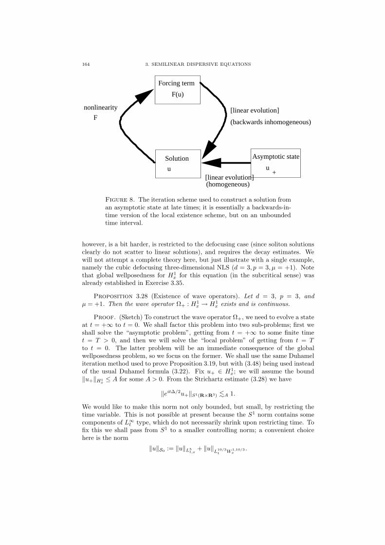
164 3. SEMILINEAR DISPERSIVE EQUATIONS
Forcing term
Solution
u
F(u)
Asymptotic state
u+
[linear evolution](homogeneous)
(backwards inhomogeneous)
[linear evolution]nonlinearity
F
Figure 8. The iteration scheme used to construct a solution froman asymptotic state at late times; it is essentially a backwards-in-time version of the local existence scheme, but on an unboundedtime interval.
however, is a bit harder, is restricted to the defocusing case (since soliton solutionsclearly do not scatter to linear solutions), and requires the decay estimates. Wewill not attempt a complete theory here, but just illustrate with a single example,namely the cubic defocusing three-dimensional NLS (d = 3, p = 3, µ = +1). Notethat global wellposedness for H1
x for this equation (in the subcritical sense) wasalready established in Exercise 3.35.
Proposition 3.28 (Existence of wave operators). Let d = 3, p = 3, andµ = +1. Then the wave operator Ω+ : H1
x → H1x exists and is continuous.
Proof. (Sketch) To construct the wave operator Ω+, we need to evolve a stateat t = +∞ to t = 0. We shall factor this problem into two sub-problems; first weshall solve the “asymptotic problem”, getting from t = +∞ to some finite timet = T > 0, and then we will solve the “local problem” of getting from t = Tto t = 0. The latter problem will be an immediate consequence of the globalwellposedness problem, so we focus on the former. We shall use the same Duhameliteration method used to prove Proposition 3.19, but with (3.48) being used insteadof the usual Duhamel formula (3.22). Fix u+ ∈ H1
x; we will assume the bound‖u+‖H1
x≤ A for some A > 0. From the Strichartz estimate (3.28) we have
‖eit∆/2u+‖S1(R×R3) .A 1.
We would like to make this norm not only bounded, but small, by restricting thetime variable. This is not possible at present because the S1 norm contains somecomponents of L∞
t type, which do not necessarily shrink upon restricting time. Tofix this we shall pass from S1 to a smaller controlling norm; a convenient choicehere is the norm
‖u‖S0 := ‖u‖L5t,x
+ ‖u‖L
10/3t W
1,10/3x
.
3.6. SCATTERING THEORY 165
From Sobolev embedding we have
‖eit∆/2u+‖S0(R×R3) . ‖eit∆/2u+‖L5tW
1,30/11x (R×R3)
+ ‖eit∆/2u+‖L10/3t W
1,10/3x (R×R3)
. ‖eit∆/2u+‖S1(R×R3)
.A 1.
Let ε > 0 be a small absolute constant to be chosen later. If we set T = T (u+)large enough, we see from monotone convergence that
‖eit∆/2u+‖S0([T,+∞)×R3) ≤ ε.
We now solve (3.48) in the spacetime slab [T,+∞) × R3 by iteration, keepingthe iterates bounded in S1([T,+∞) × R3) and small in S0, and the nonlinearity
|u|p−1u small in L10/7t W
1,10/7x ([T,+∞)×R3). This constructs a unique solution u ∈
S1([T,+∞)×R3) to (3.48), which can be shown to be a strong H1x solution to (3.1)
in this interval by a variant of Exercise 3.10. Using the global H1x-wellposedness
theory, one can then extend this solution uniquely to S1([0,+∞) × R3), and inparticular u will take some value u0 = u(0) ∈ H1
x at time t = 0. This givesexistence of the wave map; continuity can be established by concatenating thecontinuity given from the above iteration scheme in the interval [T,+∞) with thecontinuity arising from the global wellposedness in the interval [0, T ]; note that thetime T can be chosen to be uniform under small H1
x perturbations in u+ thanks tothe Strichartz estimates. The uniqueness can be made to be unconditional (in thecategory of strong H1
x solutions) by arguing as in Exercise 3.17.
Remark 3.29. The above argument shows that (perhaps unintuitively) it isin fact easier to evolve from an asymptotic state at t = +∞ to a large finite timet = T , than it is to evolve from t = T down to t = 0, as the former does noteven require energy conservation or the defocusing sign of the nonlinearity. Thereason for this is that in the asymptotic regime t → +∞, the asymptotic state isso dispersed that the nonlinear effects are extremely weak; it is only at time T andbelow that the solution reaches sufficient levels of concentration that one must startpaying more serious attention to the nonlinearity.
Now we establish asymptotic completeness. For pedagogical purposes we shallsplit the argument into three parts. First we begin with a conditional result, thatshows that asymptotic completeness is implied by a certain spacetime bound; thisis a purely perturbative argument that does not require any decay estimates. Then,we show that this rather strong spacetime bound is implied by a seemingly weakerspacetime bound. Finally, we use the decay estimates of the previous section toestablish that spacetime bound.
Proposition 3.30 (Spacetime bound implies asymptotic completeness). Letd = 3, p = 3, and µ = +1. Suppose that there exists a bound of the form
(3.49) ‖u‖S1(R×R3) .‖u0‖H1x
1
for all H1x-wellposed solutions to (3.1) (thus we assume that the nonlinear equation
obeys the same type of global Strichartz estimate as the linear equation). Then thewave operator Ω+ is surjective from H1
x to H1x, and the inverse Ω−1
+ is continuous.(In conjunction with Proposition 3.28, this implies that Ω+ is a homeomorphismfrom H1
x to itself.)
166 3. SEMILINEAR DISPERSIVE EQUATIONS
Proof. We shall demonstrate the surjectivity here, and leave the continuityto an exercise. We need to show that for any u0 ∈ H1
x, the global H1x-wellposed
solution u to (3.1) scatters in H1x; by the preceding discussion, this is equiva-
lent to the conditional convergence of the integral∫ ∞0e−it∆/2(|u(t)|2u(t)) dt in
H1x. By Strichartz estimates (e.g. (3.28)), it will suffice to show that |u|2u lies
in N1(R × R3). But from the Leibnitz rule and Holder’s inequality, followed bySobolev embedding we have
‖|u|2u‖N1(R×R3) .1∑
k=0
‖∇k(|u|2u)‖L
10/7t,x (R×R3)
.1∑
k=0
‖|u|2|∇ku|‖L
10/7t,x (R×R3)
. ‖u‖2L5
t,x‖u‖
L10/3t W
1,10/3x (R×R3)
. ‖u‖3S1(R×R3)
and the claim follows by (3.49).
Proposition 3.31 (Weak spacetime bound implies strong spacetime bound).Let d = 3, p = 3, and µ = +1. Suppose that there exists a bound of the form
(3.50) ‖u‖Lqt,x(R×R3) .‖u0‖H1
x1
for all H1x-wellposed solutions to (3.1) and some fixed 10/3 ≤ q ≤ 10. Then we
have (3.49).
Note that Sobolev embedding shows that the Lqx norm is controlled by the S1
norm. The S1 norm is ostensibly a stronger norm as it also controls one derivativeof the solution, but the point is that Strichartz estimates will allow one to controlthis stronger norm by the weaker norm (and the energy). This bootstrappingphenomenon is typical for any subcritical equation (reflecting a certain amountof “room” in the iteration argument); for critical equations, the situation is moredelicate as the relevant Strichartz norm is now scale-invariant and thus can onlybe controlled by other scale-invariant quantities; see Exercise 3.51. One can alsocombine this result with persistence of regularity results such as Proposition 3.11,giving in particular the bound
‖u‖C0tH
sx(R×R3) .s,‖u0‖H1
x‖u0‖Hs
x(R3)
for any s ≥ 0 for which the right-hand side is finite.
Proof. Let u be an H1x-wellposed solution to (3.1). We shall apply a pertur-
bative argument; to do this, we need the solution u to be made small in some sense.This shall be accomplished by partitioning the time axis37.
Let ε = ε(‖u0‖H1x) > 0 be a small number to be chosen later. Using (3.50), we
can divide the time axis R into Oε,q,‖u0‖H1x(1) intervals I, such that on each such
37This is very similar to how one iterates a local existence result to a global one, as in Figure
7. A key difference is that the time intervals considered here can be arbitrarily large or eveninfinite. In practice, this means that we are no longer permitted to use Holder in time (exceptperhaps on some exceptionally short intervals), as we generally cannot afford to lose a power ofthe length of the time interval.

3.6. SCATTERING THEORY 167
interval we have
(3.51) ‖u‖Lqx(I×R3) ≤ ε.
Now fix one of these intervals I, say I = [t0, t1]. From (3.28) we have
‖u‖S1(I×R3) . ‖u(t0)‖H1x(R3) + ‖|u|2u‖N1(I×R3).
From energy conservation we have ‖u(t0)‖H1x(R3) = O‖u0‖H1
x(1). Now we argue as
in the proof of Proposition 3.30. Estimating the N1 norm by the L10/7t W
1,10/7x
norm and using the Leibnitz rule and Holder inequality, we see that
‖|u|2u‖N1(I×R3) .1∑
k=0
‖|u|2|∇ku|‖L
10/7t,x (I×R3)
. ‖u‖2L5
t,x(I×R3)‖u‖L10/3t W 1,10/3(I×R3)
. ‖u‖2L5
t,x(I×R3)‖u‖S1(I×R3).
Now from the definition of S1 and Sobolev embedding we have
‖u‖Lrt,x(I×R3) . ‖u‖S1(I×R3)
for all 10/3 ≤ r ≤ 10. Interpolating this with (3.51) we obtain
‖u‖L5t,x(I×R3) . εα‖u‖1−α
S1(I×R3)
for some 0 < α < 1 depending on q. Combining all these estimates we obtain
‖u‖S1(I×R3) . O‖u0‖H1x(1) + εα‖u‖1−α
S1(I×R3).
If we choose ε sufficiently small depending on ‖u0‖H1x, then standard continuity
arguments (see Exercise 1.21) yields
‖u‖S1(I×R3) = O‖u0‖H1x(1).
Summing this over all of the intervals I we obtain (3.49) as desired.
It thus remains to establish the spacetime bound (3.50). In the case of spher-ically symmetric solutions, one can combine the ordinary Morawetz inequality(3.39), which in this case gives
∫
R
∫
R3
|u(t, x)|4|x| dxdt .‖u0‖H1
x1,
with the radial Sobolev inequality (Exercise A.19), which when combined with theconservation of mass and energy give
‖u(t, x)|x|‖L∞t L∞
x (R×R3) .‖u0‖H1x
1.
Multiplying the two gives
‖u‖L5t,x(R×R3) .‖u0‖H1
x1,
which is of the desired form (3.50) with q = 5. Note how the Morawetz inequalityprovides the decay near the origin, while the radial Sobolev inequality provides thedecay away from the origin. In the non-radial case, we cannot run this argumentso easily (though see [Bou6]); however the interaction Morawetz inequality (3.43)yields (3.50) immediately (with q = 4).
The above types of arguments are known to give scattering results in H1x for
defocusing NLS equations which are strictly between the H1x-critical and L2
x-critical
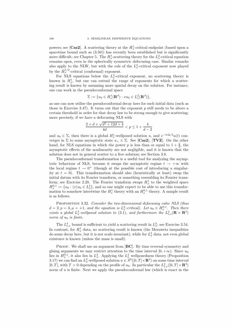
168 3. SEMILINEAR DISPERSIVE EQUATIONS
powers; see [Caz2]. A scattering theory at the H1x-critical endpoint (based upon a
spacetime bound such as (3.50)) has recently been established but is significantlymore difficult; see Chapter 5. The H1
x-scattering theory for the L2x-critical equation
remains open, even in the spherically symmetric defocusing case. Similar remarksalso apply to the NLW, but with the role of the L2
x-critical exponent now played
by the H1/2x -critical (conformal) exponent.
For NLS equations below the L2x-critical exponent, no scattering theory is
known in H1x, but one can extend the range of exponents for which a scatter-
ing result is known by assuming more spatial decay on the solution. For instance,one can work in the pseudoconformal space
Σ := u0 ∈ H1x(R
d) : xu0 ∈ L2x(R
d),as one can now utilise the pseudoconformal decay laws for such initial data (such asthose in Exercise 3.47). It turns out that the exponent p still needs to be above acertain threshold in order for that decay law to be strong enough to give scattering;more precisely, if we have a defocusing NLS with
2 + d+√d2 + 12d+ 4
4d< p ≤ 1 +
4
d− 2
and u0 ∈ Σ, then there is a global H1x-wellposed solution u, and e−it∆/2u(t) con-
verges in Σ to some asymptotic state u+ ∈ Σ. See [Caz2], [TVZ]. On the otherhand, for NLS equations in which the power p is less than or equal to 1 + 2
d , theasymptotic effects of the nonlinearity are not negligible, and it is known that thesolution does not in general scatter to a free solution; see Section 3.8.
The pseudoconformal transformation is a useful tool for analyzing the asymp-totic behaviour of NLS, because it swaps the asymptotic regime t → +∞ withthe local regime t → 0+ (though at the possible cost of introducing a singular-ity at t = 0). This transformation should also (heuristically at least) swap theinitial datum with its Fourier transform, or something resembling its Fourier trans-form; see Exercise 2.28. The Fourier transform swaps H1
x to the weighted spaceH0,1x := u0 : 〈x〉u0 ∈ L2
x, and so one might expect to be able to use this transfor-mation to somehow intertwine the H1
x theory with an H0,1x theory. A sample result
is as follows.
Proposition 3.32. Consider the two-dimensional defocusing cubic NLS (thusd = 2, p = 3, µ = +1, and the equation is L2
x-critical). Let u0 ∈ H0,1x . Then there
exists a global L2x-wellposed solution to (3.1), and furthermore the L4
t,x(R × R3)norm of u0 is finite.
The L4t,x bound is sufficient to yield a scattering result in L2
x; see Exercise 3.54.
In contrast, for H1x data, no scattering result is known (the Morawetz inequalities
do some decay here, but it is not scale-invariant), while for L2x data, not even global
existence is known (unless the mass is small).
Proof. We shall use an argument from [BC]. By time reversal symmetry andgluing arguments we may restrict attention to the time interval [0,+∞). Since u0
lies in H0,1x , it also lies in L2
x. Applying the L2x wellposedness theory (Proposition
3.17) we can find an L2x-wellposed solution u ∈ S0([0, T ]×R3) on some time interval
[0, T ], with T > 0 depending on the profile of u0. In particular the L4t,x([0, T ]×R3)
norm of u is finite. Next we apply the pseudoconformal law (which is exact in the
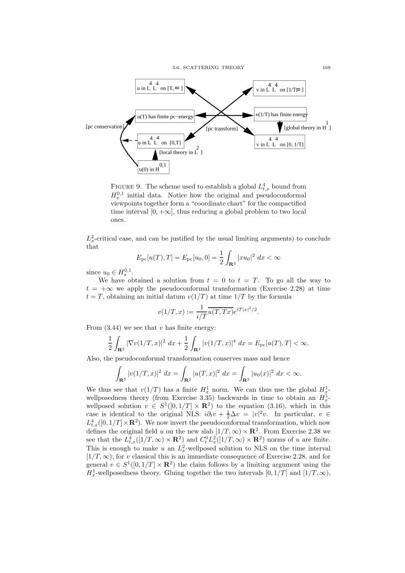
3.6. SCATTERING THEORY 169
u in L L on [0,T]4 4
v in L L on [0, 1/T]4 4
4
u(0) in H0,1
u(T) has finite pc−energy
u in L L on [T, ] v in L L on [1/T, ]4 48
4
[local theory in L ]2
8
[global theory in H ]1
[pc transform]
v(1/T) has finite energy
[pc conservation]
Figure 9. The scheme used to establish a global L4t,x bound from
H0,1x initial data. Notice how the original and pseudoconformal
viewpoints together form a “coordinate chart” for the compactifiedtime interval [0,+∞], thus reducing a global problem to two localones.
L2x-critical case, and can be justified by the usual limiting arguments) to conclude
that
Epc[u(T ), T ] = Epc[u0, 0] =1
2
∫
R2
|xu0|2 dx <∞
since u0 ∈ H0,1x .
We have obtained a solution from t = 0 to t = T . To go all the way tot = +∞ we apply the pseudoconformal transformation (Exercise 2.28) at timet = T , obtaining an initial datum v(1/T ) at time 1/T by the formula
v(1/T, x) :=1
i/Tu(T, Tx)eiT |x|2/2.
From (3.44) we see that v has finite energy:
1
2
∫
R2
|∇v(1/T, x)|2 dx+1
2
∫
R2
|v(1/T, x)|4 dx = Epc[u(T ), T ] <∞.
Also, the pseudoconformal transformation conserves mass and hence∫
R2
|v(1/T, x)|2 dx =
∫
R2
|u(T, x)|2 dx =
∫
R2
|u0(x)|2 dx <∞.
We thus see that v(1/T ) has a finite H1x norm. We can thus use the global H1
x-wellposedness theory (from Exercise 3.35) backwards in time to obtain an H1
x-wellposed solution v ∈ S1([0, 1/T ] × R2) to the equation (3.16), which in thiscase is identical to the original NLS: i∂tv + 1
2∆v = |v|2v. In particular, v ∈L4t,x([0, 1/T ]×R2). We now invert the pseudoconformal transformation, which now
defines the original field u on the new slab [1/T,∞) × R2. From Exercise 2.38 wesee that the L4
t,x([1/T,∞) × R2) and C0t L
2x([1/T,∞) × R2) norms of u are finite.
This is enough to make u an L2x-wellposed solution to NLS on the time interval
[1/T,∞); for v classical this is an immediate consequence of Exercise 2.28, and forgeneral v ∈ S1([0, 1/T ] × R2) the claim follows by a limiting argument using theH1x-wellposedness theory. Gluing together the two intervals [0, 1/T ] and [1/T,∞),

170 3. SEMILINEAR DISPERSIVE EQUATIONS
we have obtained a global L4t,x([0,+∞) × R2) solution u to (3.1) as desired. We
summarise the above argument in Figure 9.
Remark 3.33. One can go through the above argument and extract an explicitbound on the global L4
t,x norm of the solution u, but it depends on the profile of the
initial datum u0 and not just on itsH0,1x norm (as this is what determines how small
T is). Indeed, if one could obtain a bound depending only in the H0,1x norm then
the scaling invariance and a limiting argument would allow one to replaceH0,1x with
L2x, which would lead to the (still open) result that one has global wellposedness
and scattering in L2x for this equation. The above argument can also be generalised,
linking a wellposedness theory in Hsx to a scattering theory in H0,s for any s ≥ 0
and any L2x-critical equation; see [BC].
Observe how in the above argument, the pseudoconformal transformation wasused to convert an asymptotic time horizon t = +∞ to a finite time horizon t = 0,thus allowing one to use local theory to obtain asymptotic control of the solu-tion. There is a somewhat similar trick for wave equations known as conformalcompactification, in which one applies a conformal transformation of Minkowskispacetime to a pre-compact Lorentzian manifold (the “Penrose diamond”). Inone dimension d = 1, this compactification is especially simple in null coordinatesu := t+x, v := t−x, as it is given simply by (u, v) 7→ (tan−1 u, tan−1 v), thus map-ping R1+1 to the diamond-shaped region (t, x) ∈ R1+1 : |t+ x|, |t− x| < π/2. Ifthe equation is of a suitable type (it typically must obey some sort of “null condi-tion”, or the nonlinearity must be sufficiently high order), then this transformationdoes not introduce any severe singularities at the boundary of the diamond (cf.(3.16) in the case p < pL2
x), and one can use local theory on the Penrose diamond
to obtain a transformed solution on the entire diamond (if the datum is sufficientlysmall, smooth, and decaying), and then by inverting the conformal compactifica-tion one obtains a global solution in Minkowski space. Typically the transformedsolution extends to the boundary of the Penrose diamond and beyond, which oftenleads to scattering-type behaviour for the original solution. See [Chr].
Several of the above methods can also be used to establish various scatteringresults for NLW; the conformal conservation law, Morawetz estimates, the vectorfields method, and the conformal compactification methods are particularly useful.Because of finite speed of propagation, one can often reduce the case of compactlysupported data. We will not discuss these results here, except in the energy-criticalcase which we treat in see Section 5.1, and refer the reader to [Stra], [GV6], [BZS],[GV5], [Nak3], [Hid].
Exercise 3.49. Complete the proof of Proposition 3.28. (Full details can alsobe found in [Caz2].)
Exercise 3.50. Establish the continuity component of Proposition 3.30. (Onemay need to divide the time axis into intervals on which certain spacetime norms aresmall, in order that the perturbative argument can apply to give local continuity.Then concatenate the results to obtain global continuity.)
Exercise 3.51. Suppose one replaces the H1x-subcritical cubic NLS in Propo-
sition 3.31 with the H1x-critical quintic NLS (so d = 3, p = 5, µ = +1). Show that
one can still prove this Proposition if one fixes q = 10 (this is the unique value ofq which is invariant under the scaling symmetry of the equation).

3.7. STABILITY THEORY 171
Exercise 3.52. Suppose one is working with a global H1x(R
3)-wellposed so-lution u to either the cubic or quintic three-dimensional NLS (with either sign ofnonlinearity). Suppose it is known that the potential energy 1
p+1
∫R3 |u(t, x)|p+1 dx
goes to zero as t→ ∞. Conclude that the solution scatters in H1x to an asymptotic
state eit∆/2u+. (This is yet another affirmation of Principle 3.24.)
Exercise 3.53 (Blowup criterion for H1x-critical NLS). Suppose that u ∈
C0t,locH
1x([0, T∗)×R3) is a strong H1
x solution to quintic NLS (so d = 3 and p = 5)which cannot be continued beyond a finite time T∗ as a strong solution. Show thatthe L10
t,x([0, T∗)×R3) norm of u is infinite. (Hint: argue by contradiction and obtain
an S1([0, T∗) × R3) bound on u. Conclude that for times t close to T , both thelinear and nonlinear evolution of u(t) will be small in L10
t,x([t, T∗)×R3), and hence
for L10t,x([t, T∗ + ε)×R3) for some ε > 0, contradicting the hypothesis that T∗ is the
maximal time of existence.)
Exercise 3.54. Consider the two-dimensional defocusing cubic NLS (thus d =2, p = 3, µ = +1). Show that if a global L2
x-wellposed solution u is known to havefinite L4
t,x(R×R2) norm, then e−it∆/2u(t) converges in L2x to an asymptotic state
u+ ∈ L2x as t→ +∞.
3.7. Stability theory
True life is not lived where great external changes take place - wherepeople move about, clash, fight, and slay one another - it is livedonly where these tiny, tiny, infinitesimally small changes occur.(Leo Tolstoy, “Why Do People Intoxicate Themselves?”)
The differential equations that one studies in mathematics, such as NLS andNLW, often arise from physics as simplified models for more complicated systems.In reality, the actual equations that govern a physical system will not evolve bythese model equations exactly, but will contain some additional terms. For sakeof discussion let us fix the model equation to be the NLS (3.1). Instead of solvingNLS, the true system may be governed by a field u which obeys a perturbed NLS
(3.52) i∂tu+1
2∆u = µ|u|p−1u+ e; u(t0) = u0 + e0
where the forcing term e = e(t, x) and the initial datum error e0 = e0(x) are small,and possibly depending on u and on some external forces38. It is thus of interest todevelop a stability theory for equations such as NLS, which would guarantee that thesolution to a perturbed NLS does not deviate too far from the solution to the actualNLS if e and e0 are small some suitable norms. Note that this would generalisethe property of continuous dependence of the data, which is already given by thewellposedness theory and corresponds to the special case e = 0. It also generalisesthe uniqueness theory, which can be viewed as the case e = e0 = 0. A strongstability theory lends confidence as to the robustness of the results obtained for themodel equation. Conversely, if a PDE is known to be very unstable then this would
38The field of stochastic partial differential equations studies such equations with the as-sumption that e is some stochastic field, e.g. Gaussian white noise. These random fluctuations
often serve to regularise the behaviour of the equation and keep it well-behaved even when thedeterministic equation is not known to be wellposed. However, we shall focus on the determin-istic theory in which e is fixed, which is the case needed for applications such as construction ofsolutions via approximate solutions.

172 3. SEMILINEAR DISPERSIVE EQUATIONS
cast doubt on the ability of that PDE to accurately simulate (either numerically ortheoretically) a real-life system, except perhaps in some stochastic sense.
A stability theory is also useful to have in the analysis of PDE. It opens up avery useful strategy for constructing solutions u to an equation such as NLS, byfirst constructing an approximate solution u, for which i∂tu + 1
2∆u is very close
to µ|u|p−1u and u(t0) ≈ u0. In other words, an approximate solution to NLS isnothing more than an exact solution to the perturbed NLS (3.52) for some small eand e0. Stability theory can then let us pass from the approximate solution u to anearby exact solution u to the unperturbed NLS. This approach is quite powerful,because it is much easier to construct approximate solutions than exact solutions,for instance by asymptotic expansions39, or by omitting certain terms from anequation that one believes to be negligible and then solving the reduced equation;see Section 3.8 below. To give another example, while the superposition of twosolutions to a nonlinear equation will not in general yield another solution to thatequation, such a superposition is often an approximate solution to the equation if thetwo component solutions are sufficiently “separated”, either in space or frequency.This strategy can be used for instance to construct multisoliton solutions, and isalso the main reason why the “induction on energy” strategy that we shall introducein Chapter 5 is so powerful.
Fortunately, any equation with a good wellposedness theory is also likely tohave a good stability theory, by modifying the arguments used to prove wellposed-ness suitably; indeed the stability theory is in many ways the culmination of theperturbation theory methods. The main trick (which we have already seen with theuniqueness and continuity theory) is to look at the difference equation between theapproximate solution u and the exact solution40, and then solve this difference equa-tion using the same types of techniques and estimates used for the wellposednesstheory. Specifically, if we set u = u+ v, then v solves the difference equation
(3.53) i∂tv +1
2∆v = µ(|u+ v|p−1(u+ v) − |u|p−1u) + e; v(t0) = e0.
Thus the initial datum of v is small. As for the nonlinearity, we can use Taylorexpansion to expand
µ(|u+v|p−1(u+v)−|u|p−1u)+e = O(|u|p−1|v|)+O(|u|p−2|v|2)+. . .+O(|v|p)+O(|e|).assuming for simplicity that we are in the algebraic case where p is an odd integer.In practice, if e and e0 are both small, then we expect v to be small also, andthe dominant terms in the nonlinearity will be the terms O(|u|p−1|v|) which arelinear in v. These terms can be dealt with for short times by iterative argumentsbased on the Duhamel formula, as well as estimates such as Strichartz estimates; for
39In particular, the theory of nonlinear geometric optics proceeds in this fashion, constructingsolutions to an equation by first creating an ansatz consisting of an asymptotic series with certainamplitude and phase parameters. One then solves for these amplitudes and phases in order tomake the partial sums of this series an approximate solution to the original equation, and then usessome stability theory to pass to an exact solution. These methods are very useful in constructinglarge classes of interesting solutions to many PDE, though they tend to require the initial data tobe of a special form and are unsuited for the Cauchy problem with generic Hs
x initial data. Dueto limitations of space we will not be able to discuss this important technique in this text.
40This assumes that the exact solution u exists for at least as long as the approximate solutionu. In practice one can establish this by a continuity argument or by a suitable iteration of thewellposedness theory.

3.7. STABILITY THEORY 173
Initial errore0
Error in approximatesolution
e
Difference insolutions
v
Difference inforcing terms
F(u+v) − F(u)
Exact solutionu
Linear evolution
(homogeneous)
(inhomogeneous)Linear evolution
Nonlinearity
F
Figure 10. The difference scheme for an approximate perturba-tion u = u + v to an exact solution u. This scheme can also bereversed to convert an approximate solution u to an exact solutionu = u− v (by replacing F (u+ v) − F (u) with F (u) − F (u− v)).
longer times, one can use energy methods41, combined with tools such as Gronwall’sinequality, to try to keep control of the solution.
To illustrate the method, we shall consider asymptotics of one-dimensionaldefocusing NLS in the “short range” case p > 3. (The “critical range” case p = 3and the “long range” case p < 3 are significantly more interesting, but also moredifficult technically.) Applying the pseudoconformal transformation as in (3.16),we obtain the equation
(3.54) i∂tv +1
2∂xxv =
1
t(5−p)/2|v|p−1v
for 3 < p < 5, which is obtained from the one-dimensional defocusing NLS via thepseudoconformal transformation (see (3.16)). To construct solutions near t = 0,we first omit the dispersive term 1
2∂xxv (using the intuition that this term will
be dominated by the singular nonlinearity 1t(5−p)/2 |v|2v for very small times t) and
solve the simpler equation
(3.55) i∂tv =1
t(5−p)/2|v|2v.
This equation just the ODE (3.17), and can be solved explicitly as
(3.56) v(t, x) = εe−i2
p−3 ε2|ψ(x)|2t(p−3)/2
ψ(x)
41In some cases, when the exact solution u is an explicit form such as a soliton, one can use
more advanced spectral analysis of the linearised equation i∂tv + 12∆v = O(|u|p−1|v|) to obtain
long-time control of the solution; this is an important tool in the theory of stability of solitons andmultisolitons. However, such spectral methods are currently unavailable for more general classesu of solution.

174 3. SEMILINEAR DISPERSIVE EQUATIONS
for any complex-valued function ψ(x), and 0 < ε < 1 is a small parameter we haveintroduced to allow v to be small (compare with (3.18)). Thus, if ε is small, weexpect the original PDE (3.54) to have solutions which are approximately of theform (3.55). This can be established as follows.
Proposition 3.34. Let ψ ∈ Sx(R) and 0 < ε ≪ 1. If ε is sufficiently smalldepending on ψ, then we have a solution v to (3.54) on the slab (0, 1)×R obeyingthe bounds
‖v(t) − v(t)‖H1x
.ψ εt
for all 0 < t < 1, where v was defined in (3.56).
Proof. To construct v, we use the ansatz v = v+w. Subtracting (3.55) from(3.54), we see that w needs to solve the equation
i∂tw +1
2∂xxw =
1
t(5−p)/2(F (v + w) − F (v)) − ∂xxv
where F (z) := |z|p−1z. We set initial datum w(0) = 0, and write the equation inintegral form as w = Φ(w), where Φ is the nonlinear operator
Φ(w) =
∫ t
0
1
(t′)(5−p)/2(F (v(t′) + w(t′)) − F (v(t′))) − ∂xxv(t
′) dt′.
One can use energy estimates to verify that Φ is a contraction on the set tu :‖u‖C0
tH1x([0,1]×R) .ψ ε, if ε is sufficiently small depending on ψ; we leave this as
an exercise. The claim now follows from the contraction mapping principle.
Informally, the above proposition gives the approximation
v(t, x) = εe−i2
p−3ε2|ψ(x)|2t(p−3)/2
ψ(x) + l.o.t.
for 0 < t < 1, where the lower order terms go to zero in a suitable sense as t → 0.Inverting the pseudoconformal transformation, one obtains
(3.57) u(t, x) = ε1
(it)d/2exp(
i|x|22t
+2
p− 3ε2|ψ(x/t)|2t(p−3)/2)ψ(x/t) + l.o.t.
for 1 < t < ∞, where the lower order terms go to zero in a suitable sense as t →+∞. A similar argument applied to the linear Schrodinger equation (or using thefundamental solution) allows one to construct a solution ulin to the linear equationwith the asymptotics
ulin(t, x) = ε1
(it)d/2exp(
i|x|22t
)ψ(x/t) + l.o.t.
Because we are in the short-range case p > 3, we can thus conclude that u(t)−ulin(t)converges to zero in certain norms (for instance, it converges in Hs
x(R) for any s).This suggests that the short-range case, one has scattering, at least for certain typesof initial data. In the critical-range case p = 3 or the long-range case p > 3, it turnsout that one can still construct solutions to NLS of the form (3.57); the argumentsare similar though the singular nature of (3.54) now presents some delicate issues(cf. Exercise 1.19); see [Oza], [GO], [HN], [CCT] for some resolutions of this issue.These solutions fail to scatter to a solution to the linear Schrodinger equation in anyHsx norm; thus long-range and critical-range equations do not exhibit scattering to
the linear solution (this was first observed in [Gla]). However one can still hope to

3.7. STABILITY THEORY 175
establish a modified scattering result, in which the approximating solution is not alinear solution, but rather a phase-shifted linear solution; see the above references.
Next, we illustrate how Gronwall type inequalities can be used to obtain sta-bility for longer times than a simple iteration method (such as that given above)would give. The time interval on which one has non-trivial control is only extendedby a logarithmic factor, but this is sometimes sufficient for applications. It wouldbe of great interest to derive stability estimates on even longer intervals, perhapsby adapting the theory of Nekhoroshev stability from ODE, but this seems to be adifficult task (see [BK]).
Proposition 3.35. Let ψ ∈ Sx(R) and let 0 < ε≪ 1 be a small number. Then
there exists a time T ∼ψ log1/3 1ε and a strong H1
x solution u ∈ C0tH
1x([0, T ] × R)
to the small dispersion NLS
(3.58) i∂tu+ε2
2∂xxu = |u|2u; u(0) = ψ
such that ‖u− u‖C0tH
1x([0,T ]×R) .ψ ε, where
u(t, x) := e−i|ψ(x)|2tψ(x)
is the explicit solution to the ODE
i∂tu = |u|2u; u(0) = ψ.
Proof. From (a rescaled version of) Proposition 3.23 we know that a strongH1x solution u to (3.58) exists globally in time42 Writing u = u+ w, we see that w
solves the equation
i∂tw + ε2∂xxw = (|(u + w)|2(u+ w) − |u|2u) − ε2
2∂xxu; w(0) = 0
which we write in Duhamel form as
w(t) =
∫ t
0
eiε2(t−t′)∂xx [(|(u + w)|2(u + w) − |u|2u) − ε2
2∂xxu](t
′) dt′.
We take H1x norms of both sides, and use the fact that eiε
2(t−t′)∂xx is bounded inH1x, to obtain
‖w(t)‖H1x≤
∫ t
0
‖|(u+ w)|2(u+ w)(t′) − |u|2u(t′)‖H1x
+ε2
2‖∂xxu(t′)‖H1
xdt′.
A direct computation shows that
‖u(t′)‖H1x
.ψ 〈t′〉; ‖∂xxu(t′)‖H1x
.ψ 〈t′〉3
while a computation using the algebra property of H1x (see Lemma A.8) gives
‖|(u+ w)|2(u+ w)(t′) − |u|2u(t′)‖H1x
. ‖w(t′)‖H1x(‖u(t′)‖H1
x+ ‖w(t′)‖H1
x)2.
Putting this all together, we obtain the bound
‖w(t)‖H1x
.ψ ε2〈t〉4 +
∫ t
0
〈t〉2‖w(t′)‖H1x
+ ‖w(t′)‖3H1
xdt′.
42This global wellposedness is convenient for the argument, but not absolutely necessary;the energy bounds we obtain in the proof, combined with the local H1
x wellposedness theory,are sufficient (via a standard continuity argument) to construct the solution u on the given timeinterval [0, T ].

176 3. SEMILINEAR DISPERSIVE EQUATIONS
v in L L10 10
v(0) in H
(large norm)
1
v in L Wlin
10 . 1,30/13
(small norm)
(large norm) (small norm) [Sobolev]
Net forcing term in N
.
e in L W
(small norm)
(small norm)
u in L W
(small norm)
(small norm)
F(u+v)−F(u) in L W
(small norm)
(large norm)
[local theory]
1
(large norm)
u in S~~
~
~
~
v in S.
[Strichartz estimates]
10 . 1,30/13[Leibnitz, Holder,
Sobolev]
2 . 1,6/5
. 1,6/5 u in C H0 .1
v in L W10 . 1,30/13
1
1
2
Figure 11. The scheme for estimating the difference v = u − uin Lemma 3.36; it is thus a rather complex variation of the usualStrichartz iteration loop for this equation (see Figure 5).
If ε is sufficiently small depending on t, a continuity argument then gives
‖w(t)‖H1x
.ψ ε2〈t〉4 exp(C〈t〉3)
for all 0 < t ≪ log1/3 1ε (cf. what one would obtain by Gronwall’s inequality by
dropping the nonlinear term ‖w(t′)‖3H1
x), and the claim follows.
In the next section we will use this proposition to obtain some illposednessresults for NLS.
Our final example of a stability theory result comes from the defocusing energy-critical three-dimensional NLS (d = 3, p = 5, µ = +1). We shall show that H1
x-wellposed solutions to this equation are stable as long as the L10
t,x norm staysbounded. We first state a preliminary result in which we assume that a certainspacetime norm on the solution is small.
Lemma 3.36 (Short-time perturbations). [CKSTT11] Let d = 3, p = 5, µ =+1. Let I be a compact interval, and let u be a field on I × R3 which is a near-solution to NLS in the sense that
(3.59) (i∂t +1
2∆)u = |u|4u+ e
for some field e. Suppose that we also have the energy bound
‖u‖L∞t H1
x(I×R3) ≤ E
for some E > 0. Let t0 ∈ I, and let u(t0) be close to u(t0) in the sense that
(3.60) ‖u(t0) − u(t0)‖H1x≤ E′
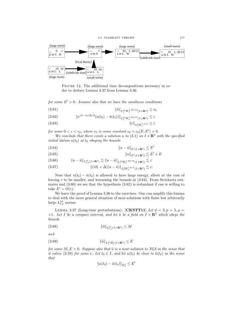
3.7. STABILITY THEORY 177
u in L~ 10
L10
u in L~ 10
L10
u in C H0 . 1~
(large norm)
1~u in S
(large norm)
(large norm)
[subdivide time]
(small norm)
[local theory][subdivide time]
u in L W~ 10 . 1, 30/13 10 . 1, 30/13
u in L W~
(large norm) (small norm)
Figure 12. The additional time decompositions necessary in or-der to deduce Lemma 3.37 from Lemma 3.36.
for some E′ > 0. Assume also that we have the smallness conditions
‖u‖L10
t W1,30/13x (I×R3)
≤ ǫ0(3.61)
‖ei(t−t0)∆/2(u(t0) − u(t0))‖L10t W
1,30/13x (I×R3)
≤ ε(3.62)
‖e‖L2
tW1,6/5x
≤ ε(3.63)
for some 0 < ε < ǫ0, where ǫ0 is some constant ǫ0 = ǫ0(E,E′) > 0.
We conclude that there exists a solution u to (3.1) on I ×R3 with the specifiedinitial datum u(t0) at t0 obeying the bounds
‖u− u‖S1(I×R3) . E′(3.64)
‖u‖S1(I×R3) . E′ + E(3.65)
‖u− u‖L10t,x(I×R3) . ‖u− u‖
L10t W
1,30/13x (I×R3)
. ε(3.66)
‖(i∂t + ∆)(u − u)‖L2
tW1,6/5x (I×R3)
. ε.(3.67)
Note that u(t0) − u(t0) is allowed to have large energy, albeit at the cost offorcing ε to be smaller, and worsening the bounds in (3.64). From Strichartz esti-mates and (3.60) we see that the hypothesis (3.62) is redundant if one is willing totake E′ = O(ε).
We leave the proof of Lemma 3.36 to the exercises. One can amplify this lemmato deal with the more general situation of near-solutions with finite but arbitrarilylarge L10
t,x norms.
Lemma 3.37 (Long-time perturbations). [CKSTT11] Let d = 3, p = 5, µ =+1. Let I be a compact interval, and let u be a field on I × R3 which obeys thebounds
(3.68) ‖u‖L10t,x(I×R3) ≤M
and
(3.69) ‖u‖L∞t H1
x(I×R3) ≤ E
for some M,E > 0. Suppose also that u is a near-solution to NLS in the sense thatit solves (3.59) for some e. Let t0 ∈ I, and let u(t0) be close to u(t0) in the sensethat
‖u(t0) − u(t0)‖H1x≤ E′

178 3. SEMILINEAR DISPERSIVE EQUATIONS
for some E′ > 0. Assume also that we have the smallness conditions,
‖ei(t−t0)∆/2(u(t0) − u(t0))‖L10t W
1,30/13x (I×R3)
≤ ε(3.70)
‖e‖L2
tW1,6/5x (I×R3)
≤ ε
for some 0 < ε < ε1, where ε1 is a small constant ε1 = ε1(E,E′,M) > 0. We
conclude there exists a solution u to (3.1) on I×R3 with the specified initial datumu(t0) at t0, and furthermore
‖u− u‖S1(I×R3) .M,E,E′ 1
‖u‖S1(I×R3) .M,E,E′ 1
‖u− u‖L10t,x(I×R3) . ‖u− u‖
L10t W
1,30/13x (I×R3)
.M,E,E′ ε.
Again, we leave the details to the exercises. This stability lemma is quitepowerful; it shows that approximate solutions can be adjusted to become exactsolutions even when the energy of both initial data and their difference are large,as long as the approximate solution is bounded (but not necessarily small) in L10
t,x
norm, and the error e is very small. It will play an important role in the largeenergy theory of this equation in Chapter 5.
In the preceding examples of stability theory, we approximated an exact solu-tion u by an explicit approximate solution u. In some cases, most notably in thestability theory of solitons and multisolitons, it is better to approximate u by a par-tially explicit approximate solution, which involves some free parameters that onehas some freedom to choose in order to make the analysis of the error terms as easyas possible. For instance, if considering perturbations u of a soliton solution such aseitτQ(x), the ansatz u = eitτQ(x)+w turns out to not be very effective (the boundson w will grow exponentially in time if one applies perturbation theory naively).Instead, a better procedure is to perform an ansatz u = eitτ+θ(t)Q(x − x(t)) + w,where θ : R → R and x : R → Rd are parameters that one can choose. Typically,one chooses these parameters in order to obtain some moment conditions on w(for instance, one could try to force w to be orthogonal to functions such as iQ or∇Q), which can improve the behaviour of the equation for w (by eliminating somedegeneracies in the linearised operator associated to Q). This reflects the fact thatperturbations to a soliton can cause that soliton to move in a significant manneralong the directions given by the symmetries of the equation, namely phase rotationand spatial translation; these are major channels of propagation for the equation asmotion in these directions does not conflict with any of the conservation laws. (Inthe case of the L2
x-critical equation, motion in the scaling direction is also possibleas it does not contradict conservation of mass.) We will not have space to devoteattention to these tools, which are fundamental in the stability theory of solitons,but see [Wei2] and many subsequent papers (e.g. [MR], [MR2], [MR3] and thereferences therein).
Exercise 3.55 (Justification of energy conservation). Let d = 3 and 1 < p < 5,µ = +1, t0 = 0, and u0 ∈ H1
x(Rd). For each ε > 0, show that there exists a global
H1x-wellposed solution u(ε) solution to the regularised NLS
i∂tu(ε) +
1
2∆u(ε) = (|u(ε)|2 + ε2)(p−1)/2u(ε); u(ε)(0) = u0
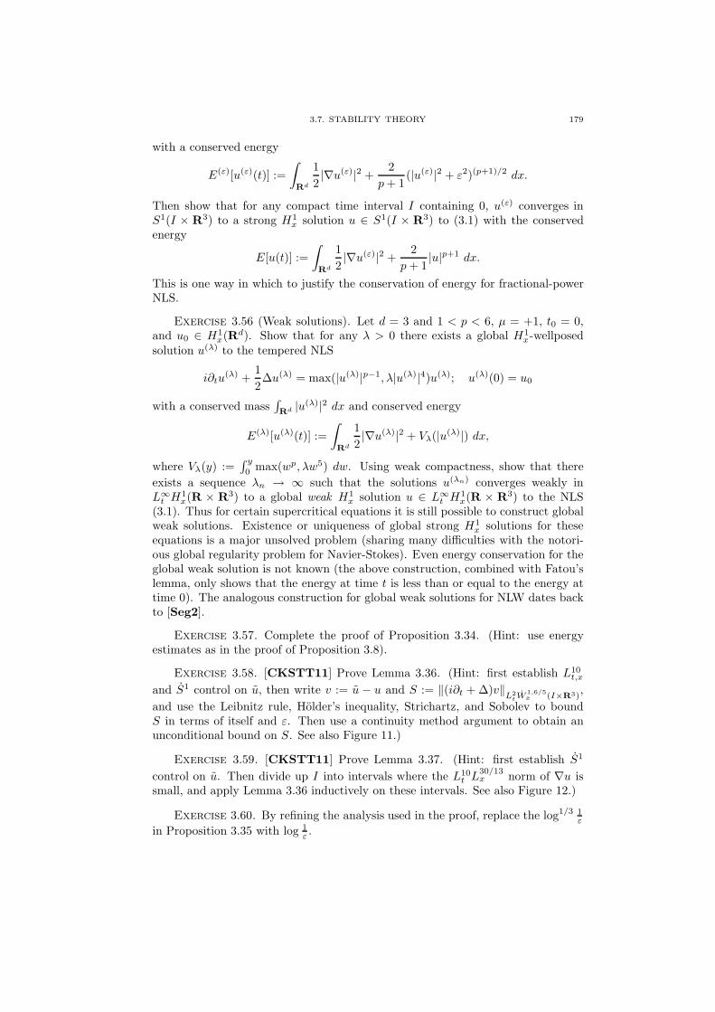
3.7. STABILITY THEORY 179
with a conserved energy
E(ε)[u(ε)(t)] :=
∫
Rd
1
2|∇u(ε)|2 +
2
p+ 1(|u(ε)|2 + ε2)(p+1)/2 dx.
Then show that for any compact time interval I containing 0, u(ε) converges inS1(I × R3) to a strong H1
x solution u ∈ S1(I × R3) to (3.1) with the conservedenergy
E[u(t)] :=
∫
Rd
1
2|∇u(ε)|2 +
2
p+ 1|u|p+1 dx.
This is one way in which to justify the conservation of energy for fractional-powerNLS.
Exercise 3.56 (Weak solutions). Let d = 3 and 1 < p < 6, µ = +1, t0 = 0,and u0 ∈ H1
x(Rd). Show that for any λ > 0 there exists a global H1
x-wellposedsolution u(λ) to the tempered NLS
i∂tu(λ) +
1
2∆u(λ) = max(|u(λ)|p−1, λ|u(λ)|4)u(λ); u(λ)(0) = u0
with a conserved mass∫Rd |u(λ)|2 dx and conserved energy
E(λ)[u(λ)(t)] :=
∫
Rd
1
2|∇u(λ)|2 + Vλ(|u(λ)|) dx,
where Vλ(y) :=∫ y0 max(wp, λw5) dw. Using weak compactness, show that there
exists a sequence λn → ∞ such that the solutions u(λn) converges weakly inL∞t H
1x(R × R3) to a global weak H1
x solution u ∈ L∞t H
1x(R × R3) to the NLS
(3.1). Thus for certain supercritical equations it is still possible to construct globalweak solutions. Existence or uniqueness of global strong H1
x solutions for theseequations is a major unsolved problem (sharing many difficulties with the notori-ous global regularity problem for Navier-Stokes). Even energy conservation for theglobal weak solution is not known (the above construction, combined with Fatou’slemma, only shows that the energy at time t is less than or equal to the energy attime 0). The analogous construction for global weak solutions for NLW dates backto [Seg2].
Exercise 3.57. Complete the proof of Proposition 3.34. (Hint: use energyestimates as in the proof of Proposition 3.8).
Exercise 3.58. [CKSTT11] Prove Lemma 3.36. (Hint: first establish L10t,x
and S1 control on u, then write v := u − u and S := ‖(i∂t + ∆)v‖L2
tW1,6/5x (I×R3)
,
and use the Leibnitz rule, Holder’s inequality, Strichartz, and Sobolev to boundS in terms of itself and ε. Then use a continuity method argument to obtain anunconditional bound on S. See also Figure 11.)
Exercise 3.59. [CKSTT11] Prove Lemma 3.37. (Hint: first establish S1
control on u. Then divide up I into intervals where the L10t L
30/13x norm of ∇u is
small, and apply Lemma 3.36 inductively on these intervals. See also Figure 12.)
Exercise 3.60. By refining the analysis used in the proof, replace the log1/3 1ε
in Proposition 3.35 with log 1ε .
180 3. SEMILINEAR DISPERSIVE EQUATIONS
Exercise 3.61. [CKSTT13] Let u ∈ C0t,locSx(R×T2) be a classical solution
to the cubic defocusing NLS i∂tu+ 12∆u = |u|2u. Using the Fourier ansatz u(t, x) =∑
k∈(2πZ)2 ei(k·x+ 1
2 |k|2t)ak(t), deduce the infinite system of ODE
(3.71) ∂ta(t) = Nt(a(t), a(t), a(t))
where a = (ak)k∈(2πZ)2 and Nt is the trilinear form
Nt(a, b, c)k :=∑
k1,k2,k3∈(2πZ)2:k1−k2+k3=k
ak1bk2ck3ei2 (|k1|2−|k2|2+|k3|2−|k4|2)t.
(Compare with (1.56)). Let K ≫ 1 be a large number, let 0 < σ < 1, and letT ≤ c(σ)K2 logK for some small c(σ) > 0 depending only on σ. Suppose we havea system b(t) = (bk(t))k∈(2πZ)2 of functions with b ∈ C1
t l1k([0, T ] × (2πZ)2) with
b(0) = a(0) which obeys the approximate equation
∂tb(t) = Nt(b(t), b(t), b(t)) + e(t)
to (3.71), where e(t) and b(t) obey the l1 bounds
‖b‖C1t l
1k([0,T ]×(2πZ)2 . K−1; sup
0≤t≤T
∫ t
0
‖∫ t
0
e(t′) dt′‖l1k
. K−1−σ.
Then if c(σ) is sufficiently small depending on σ, we have the estimate ‖a −b‖C1
t l1k([0,T ]×(2πZ)2 . K−1−σ/2. This lemma allows one to use near-solutions to NLS
in Fourier space to approximate actual solutions to NLS, and is a key ingredient inestablishing a certain weak turbulence result for this equation. See [CKSTT13].
3.8. Illposedness results
All happy families resemble one another; each unhappy family isunhappy in its own way. (Leo Tolstoy, “Anna Karenina”)
In the past few sections we have developed a wellposedness theory for severaltypes of NLS and NLW equations, for various regularities Hs
x (or Hsx × Hs−1
x ).Despite the wide variety of equations and regularities considered, the wellposed-ness theory for these equations are remarkably similar to each other, especially forsubcritical regularities. In such cases the time of existence depends only on thenorm of the data, and the solution map not only exists and is unique, but enjoysvery strong continuity properties; indeed, the solution map (from Hs
x to C0tH
sx)
is typically uniformly continuous, Lipschitz, infinitely differentiable, and even realanalytic (see for instance Exercise 3.25).
However, there are certain equations and certain regularities for which theCauchy problem does not agree with this picture, either locally or globally in time,in which case we say that that particular Cauchy problem is illposed. Unlike the sit-uation with wellposedness, the type of illposedness exhibited can vary substantiallyon the equation and on the regularity. At one extreme, there are very dramaticexamples of illposedness, such as blowup - various norms going to infinity in finitetime - beyond which no reasonably strong notion of solution can be salvaged. Atthe other extreme there are very mild examples of illposedness, where it may stillbe that the solution map exists and could even be continuous, but that the solutionmap is known to be unstable (e.g. non-uniformly-continuous or non-Lipschitz),

3.8. ILLPOSEDNESS RESULTS 181
non-differentiable, or at least non-analytic. Intermediate between these extremes43
are examples of norm explosion - when data of arbitrarily small norm can lead tosolutions of arbitrarily large norm in arbitrarily small time. This is not quite asdramatic as blowup, because a solution may still exist for each given initial datum,but it certainly does prevent any continuous dependence of the solution map on theinitial data.
For each of the types of illposedness discussed above, there are examples ofequations and regularities that exhibit that illposedness. In contrast with the well-posedness theory, which is largely based around the single technique of Duhameliteration, illposedness can be achieved by a surprisingly large number of unrelatedmethods. We will not be able to discuss all of them here, but we give a represen-tative sample. For a recent survey of techniques and results, see [Tzv].
We first discuss methods for generating blowup, by which we mean classical (orstrong) solutions which develop a significant singularity in finite time (e.g. the Hs
x
norm goes to infinity in finite time). One way to construct these solutions is viaconstruction of explicit (or nearly explicit) blowup solutions. We have already seentwo examples of this - the blowup solution (3.15) for the pseudoconformal focusingNLS and the ODE-based blowup solution (3.6) for the focusing NLW. The lattersolution has no decay in space and thus does not lie in any Hs
x × Hs−1x spaces,
however this can be rectified by a finite speed of propagation; see Exercise 3.9.In some cases, one cannot construct a blowup solution explicitly, but can cre-
ate an explicit approximate solution to the equation which blows up in finite time.One can then hope to use perturbation theory to convert this to an exact blowupsolution. This argument can be made to work, but is extremely delicate, becauseperturbation theory requires a great deal of wellposedness and stability on theequation, which is in obvious conflict with our need to make both the exact andapproximate solution to blow up in finite time. One often needs to carefully renor-malise the solution (usually via rescaling), and obtain stability control in one set ofnorms while obtaining blowup in another. See for instance [Mer], [BW] for someinstances of this approach.
In the case of the NLS, there is another, much more indirect, way to forceblowup of a solution, namely the virial argument of Glassey [Gla2], based on thenonlinear counterpart to (2.38). For simplicity let us consider a classical solutionu ∈ C∞
t,locSx(R × Rd) to an algebraic NLS. Consider the quantity
V (t) :=
∫
Rd
|x|2T00(t, x) dx =
∫
Rd
|x|2|u(t, x)|2 dx.
43There are several other “symptoms” of illposedness which we will not have space to discuss
here, including breakdown of uniqueness (either for weak or strong solutions); failure of mass orenergy conservation; loss of regularity; or examples of approximate solutions to the equation whichblowup in finite time. The reader is invited to try to list several such illposedness phenomena andrank them in approximate order of severity.
182 3. SEMILINEAR DISPERSIVE EQUATIONS
This quantity is clearly non-negative. Applying (2.35) and integration by partsrepeatedly, we obtain the virial identity
∂ttV (t) = 2
∫
Rd
Tjj(t, x) dx
=
∫
Rd
2|∇u|2 +µd(p− 1)
p+ 1|u|p+1 dx
= 4E[u] +µd(p− pL2
x)
p+ 1
∫
Rd
|u(t, x)|p+1 dx
(3.72)
where E[u] is the conserved energy and pL2x
:= 1+ 42 is the pseudoconformal power.
If we are in the L2x-critical or L2
x-supercritical focusing cases p ≥ pL2x, µ = −1, we
thus conclude the bound
∂ttV (t) ≤ 4E[u].
If the energy happens to be negative (which is possible in the focusing case µ = −1),this shows that V is a strictly concave function of t. Since V is also non-negative,we conclude that the solution can only exist classically for a finite amount of time(in either direction). This argument thus demonstrates blowup in finite time (andeven gives an upper bound on the time of existence in terms of the datum andthe energy). It can be extended to demonstrate blowup for any H1
x initial data u0
which has negative energy44 and obeys the decay condition 〈x〉u0 ∈ L2x. The decay
condition can be removed, basically by working with spatially truncated versions ofthe virial identity; see for instance [Naw]. We remark that while negative energyis a sufficient condition for blowup, it is hardly a necessary condition; for instance,the solution (3.15) has zero energy, and the solutions constructed in [BW] havepositive energy. The blowup phenomenon has been analyzed much further for theL2x-critical equation, in the vicinity of soliton solutions; see [MR], [MR2], [MR3].
For the focusing NLW, one can also exploit some positivity properties of thefundamental solution to establish successively stronger lower bounds on a solutionwhich eventually leads to blowup. One particularly striking example of this is aresult of John [Joh], who showed that for the three-dimensional focusing NLW withinitial data u(0, x) = εu0(x), ∂tu(0, x) = 0 for positive Schwartz u0 and sufficiently
small ε, one has blowup in finite time for p <√
2 and global existence for p >√
2.These results have since been generalised extensively; see for instance [GLS], [Hor].
Once one has one solution blowing up, one can use the symmetries of theequation to generate further solutions blowing up. When the regularity s is lowenough, one can use the symmetries to create classical initial data of arbitrarilysmall Hs
x norm which blow up in arbitrarily small time, which is a very strongdemonstration of illposedness in that data class Hs
x; we give some examples in theexercises.
All the known examples of blowup from classical data are for focusing equations;for many defocusing equations (e.g. H1
x-subcritical or H1x-critical defocusing NLS
or NLW) we have global existence of classical solutions. The question of whetherblowup occurs from classical data for H1
x-supercritical defocusing NLS or NLWequations is a major open problem in the subject (analogous to the Navier-Stokesglobal regularity problem) and remains very far from resolution. While blowup
44To put it another way, whenever the nonlinear component of the energy exceeds the linearcomponent, blowup occurs. Compare this with Principle 3.24.

3.8. ILLPOSEDNESS RESULTS 183
is not known for these equations, we can in many cases establish weaker formsof illposedness, which are not as dramatic as blowup but do indicate that many ofthe techniques discussed in earlier sections to establish wellposedness (e.g. iterationmethods) must necessarily fail. One of the mildest types of illposedness of this formis that of analytic illposedness, in which one demonstrates that the solution map (sayfrom Hs
x to C0tH
sx), if it exists at all, is not real analytic. In fact one typically shows
the stronger statement of Ck illposedness for some k ≥ 1, which asserts that thesolution map, if it exists, is not k-times differentiable. This is basically accomplishedby the method of Taylor expansions (i.e. power series methods). Let us illustratethis with the three-dimensional cubic defocusing NLS (d = 3, p = 3, µ = +1)with initial datum u(0) = εu0 for some fixed Schwartz u0, thus we are consideringsolutions u(ε) to the Cauchy problem
(3.73) i∂tu(ε) +
1
2∆u(ε) = |u(ε)|2u(ε); u(0) = εu0.
The global existence theory of this equation (Exercise 3.38) guarantees that thesolutions u(ε) exist and are smooth for all time. A refinement of this theory alsoshows us that u(ε) also depend smoothly on ε, uniformly on any compact timeinterval. In particular, we can obtain a Taylor expansion
u(ε)(t, x) = εu1(t, x) + ε2u2(t, x) + ε3u3(t, x) +O(ε4)
for some smooth functions u1, u2, u3 (there is no zeroth order term since u(0) isclearly zero), where the error is uniformly smooth in t, x on any compact timeinterval. We can expand both sides of (3.73) using this expansion and comparecoefficients. One learns that the first coefficient u1 is just the linear solution:
i∂tu1 +1
2∆u1 = 0; u1(0) = u0
or in other words u1(t) = eit∆/2u0. The second term u2 solves the equation
i∂tu2 +1
2∆u2 = 0; u2(0) = 0
and is hence zero. The third term u3 solves the equation
i∂tu3 +1
2∆u3 = |u1|2u1; u3(0) = 0
and is hence given by a Duhamel integral
u3(t) = −i∫ t
0
ei(t−t′)∆/2(|u1|2u1(t
′)) dt′ = −i∫ t
0
ei(t−t′)∆/2(|eit′∆/2u0|2eit
′∆/2u0) dt′.
From the Taylor expansion of u(ε) we thus have obtained the formula
d3
dε3u(ε)(t)|ε=0 = −3!i
∫ t
0
ei(t−t′)∆/2(|eit′∆/2u0|2eit
′∆/2u0) dt′.
This shows that if the map u0 7→∫ t0ei(t−t
′)∆/2(|eit′∆/2u0|2eit′∆/2u0) dt
′ is not a
bounded map from Hsx(R
3) to C0tH
sx([0, T ] × R3), then the solution map u0 7→ u
will not be a C3loc map from Hs
x(R3) to C0
tHsx([0, T ]×R3), even for data arbitrarily
close to zero in Hsx norm. This lack of boundedness can often be established by
direct computation; in this case, we can achieve this for supercritical regularitiess < sc = 1
2 (in contrast to the critical case s = sc and subcritical cases s > sc, inwhich one does have analytic wellposedness); see Exercise 3.65.

184 3. SEMILINEAR DISPERSIVE EQUATIONS
The method above is fairly general. Roughly speaking, it shows that if theDuhamel iteration scheme used to construct solutions leaves a certain space X afterfinitely many iterations, then the solution map can only have a finite amount ofdifferentiability in that space. This is not too surprising since the iteration schemeis closely akin to a power series expansion of the solution in terms of the initialdatum.
Another approach for establishing illposedness is by constructing families of ex-act solutions to the equation which are close together at time zero but far apart atother times. In some cases one can use explicit solutions such as solitons and planewave solutions, possibly after various symmetries of the equation have been applied;in other cases one needs to construct solutions by the methods of nonlinear geomet-ric optics, or more generally by constructing an approximate solution first and thenusing stability theory to perturb the approximate solution into the exact solution.A typical result obtained by this method would be that a certain solution operatorcannot be uniformly continuous from Hs
x to C0tH
sx even when the size of the datum
and time of existence are set to be small. We have already seen some examples ofthis in Exercise 3.5 and the discussion after (3.20), using explicit solutions. We nowbriefly sketch how to achieve a similar effect using the approximate solutions of thepreceding section. For sake of concreteness let us just consider the one-dimensionaldefocusing cubic NLS (d = 1, p = 3, µ = +1). Let ψ be a Schwartz function. FromProposition 3.35 we have constructed (for small ε > 0 and 1 ≤ a ≤ 2) solutions wε,a
to the small-dispersion equation i∂twε + ε2
2 ∂xxwε = |v|2wε on the slab [0, 1] × R
which has the approximate form
wε,a(t, x) = ae−ia2|ψ(x)|2tψ(x) + Oψ(ε)
for 0 ≤ t ≤ 1, where the error can be controlled in a suitable H1x sense. One can
apply the rescaling uε,a(t, x) := wε,a(t, εx) to obtain a class of solutions uε to theoriginal NLS with the approximate form
uε,a(t, x) = ae−ia2|ψ(εx)|2tψ(εx) +Oψ(ε)
where the error is now controlled in some rescaled H1x sense. One can exploit scale
invariance (3.9) and Galilean invariance (3.10) to obtain a wider class of exactsolutions uε,a,λ,v to NLS for λ > 0 and v ∈ R of the form
uε,a,λ,v(t, x) = λ−2/(p−1)aei(x·v+t|v|2
2 −a2|ψ(ε(x−vt)/λ)|2t/λ2)ψ(ε(x−vt)/λ)+Oψ(ελ−2/(p−1))
where the error has to be interpreted in a suitable norm. If s < 0 is a negativeregularity, then by making v large, and setting λ ∼ε |v|−(p−1)s/2, these solutionscan become bounded in Hs
x. By a suitable variation of the parameters ε, a, λ, v onecan then show that the solution operator to this equation cannot be uniformly con-tinuous from Hs
x to C0tH
sx, even for small times and small norm, by exploiting the
phase decoherence effect arising from the a2|ψ(ε(x−vt)/λ)|2t/λ2 term; see [CCT2]for details. Generally speaking, it is not difficult to create (for any equation andregularity) large data solutions which exhibit these types of instabilities at largetimes; the various symmetries are then used to create small data solutions whichare similarly unstable at small times. In order for this to work, one needs the reg-ularity s to be supercritical with respect to at least one of the symmetries (scaling,Galilean, or Lorentz). See [Kuk], [Leb], [BGT], [CCT], [CCT2], [CCT3] forseveral examples of this technique and further discussion.

3.8. ILLPOSEDNESS RESULTS 185
One final type of illposedness is the high-to-low frequency cascade, in whicha solution starts off initially with Fourier transform supported primarily at highfrequencies, but quickly creates a substantial presence at low frequencies. For smalls (e.g. negative s), such solutions typically have small Hs
x norm at time zerobut large Hs
x norm at later times; this norm explosion is a fairly strong form ofillposedness as it shows that the solution operator, if it exists at all, has a severesingularity in Hs
x near the zero solution. These cascading solutions can often be
constructed using the stability theory arising from a higher regularity Hs′
x . See[CCT2], [BT] for examples of this strategy.
Exercise 3.62. Let u be a classical solution to an NLW, and let
V (t) :=
∫
Rd
|x|2T00(t, x) −d− 1
2|u|2 dx.
Establish the following analogue of the virial identity for this quantity, namely
∂ttV (t) = 2E[u] +µ(d− 1)(p− p
H1/2x
)
p+ 1
∫
Rd
|u(t, x)|p+1 dx
where pH
1/2x
:= 1+ 4d−1 is the conformal power. (Note the shifting of the dimension
d by one; compare this with Exercise 3.2.) This identity is not as useful as the NLSvirial identity because the quantity V does not have a definite sign in general.
Exercise 3.63. Consider a focusing NLS with p ≥ pL2x
= 1 + 4d , and let
s < sc. Show that there exists classical data of arbitrarily small Hsx norm such that
the solution to the NLS blows up in arbitrarily small time. (Hint: use the virialidentity to create a classical solution with Schwartz initial data which blows up infinite time, and then use the scaling symmetry to rescale the blowup time to bearbitrarily small.) This illustrates the principle that one usually does not have awellposedness theory at supercritical regularities for focusing equations.
Exercise 3.64. Consider a focusing NLW and let s < sc. Show that thereexists classical data of arbitrarily small Hs
x ×Hs−1x norm such that the solution to
the NLW blows up in arbitrarily small time. (Hint: use Exercise 3.9. In the casewhen sc is negative, you may find it convenient to enforce moment conditions onthe initial data to ensure some vanishing of the Fourier coefficients near the origin.)A similar result holds for s < sl (using the Lorentz invariance instead of the scalinginvariance) but is a little trickier; see [Sog].
Exercise 3.65. Let T > 0 be arbitrary. Use a scaling argument to show that
the map u0 7→∫ t0 e
i(t−t′)∆/2(|eit′∆/2u0|2eit′∆/2u0) dt
′ is not a bounded map from
Hsx to C0
tHsx([0, T ] × R3) when s < 1/2. Conversely, use Strichartz estimates to
show that this map is bounded for s ≥ 1/2. (For sake of this exercise, you may usethe heuristic (A.15) as if it were rigorous. Alternatively, one may use Littlewood-Paley decomposition.)
Exercise 3.66. [Kat4] Consider the rather artificial nonlinear wave equationu = −|u|p for some H1
x-subcritical power 1 ≤ p < 1 + 4d−2 . Let u be a strong
H1x × L2
x solution to this equation whose initial position is supported in the ball|x| ≤ 1 and whose initial velocity is zero (for simplicity). It is possible to establishthe finite speed of propagation property for such solutions, in particular you mayassume that this solution is supported on the ball |x| ≤ 1 + t for all later times

186 3. SEMILINEAR DISPERSIVE EQUATIONS
t > 0 for which the solution exists. Show that if the integral∫Rd u(0, x) dx is
sufficiently large and positive depending on d and p, then the solution u can onlyexist for a finite amount of time in the forward direction (i.e. u cannot be astrong solution on [0,+∞)). If p < 1 + 2
d , show that one only needs the integral∫Rd u(0, x) dx to be strictly positive to achieve the same result (i.e. no largeness
hypothesis is required). Hints: obtain an integral inequality for the quantitym(t) :=∫Rd u(t, x) dx, using Holder’s inequality and finite speed of propagation. First show
that m(t) is convex and monotone increasing, and then obtain even better lowerbounds on this quantity. You may find the comparison principle, Exercise 1.7, tobe useful. For further variations on this theme, see [KTao3].
Exercise 3.67. [LSog], [Sog] Consider a focusing NLW, and let s be suchthat 0 < s < sl := d+1
4 − 1p−1 (so s is supercritical with respect to the Lorentz
invariance). Start with the explicit blowup solution (3.6) with t0 = 0 and apply aLorentz transform to it, to create a solution which blows up at the point (0, 0) but issmooth in the backwards light cone (t, x) : |x| < −t. Now work on the time slicet = −1 and localise the initial data to a neighbourhood of the ball |x| < 1 usingfinite speed of propagation, to create smooth initial data (u(−1), ∂tu(−1)) whoseHsx(R
d) × Hs−1x (Rd) norm is arbitrarily small, but which develops a singularity
at time 0. Rescaling this, we can construct data of arbitrarily small Hsx(R
d) ×Hs−1x (Rd) norm with a solution that blows up in arbitrarily small time, which
defeats any hope of a reasonable wellposedness theory at this regularity.
3.9. Almost conservation laws
The Law of conservation of energy tells us we can’t get somethingfor nothing, but we refuse to believe it. (Isaac Asimov)
We have seen how the laws of conservation of mass and energy can be usedto obtain global wellposedness results at the L2
x and H1x regularities respectively;
generally speaking, they assert that these two norms stay bounded for all time. Onemay then ask what happens to the other Hs
x norms; after all, the linear Schrodingerand wave flows preserve the Hs
x norm and Hsx × Hs−1
x norms respectively. Inparticular, once one has global wellposedness for one norm, say H1
x, one can askwhether the same wellposedness occurs for other regularities also.
Generally speaking, global wellposedness in lower norms implies global well-posedness in higher norms45, due to persistence of regularity; we have already seenseveral examples of this phenomenon in this chapter. However, while the lowerSobolev norms such as H1
x may remain bounded uniformly in time, the bounds oneobtains on higher norms such as H2
x may grow faster than this; see for instance theexponential bounds in Exercise 3.28. This reflects the fact that the persistence ofregularity arguments do not prohibit a “low-to-high frequency cascade” scenario, inwhich the energy starts off concentrated in low frequencies but moves increasinglyto higher frequencies as time progresses; it is easy to envisage a scenario of thisform where the H1
x norm stays bounded, but higher norms such as H2x go to infin-
ity. Numerical simulations have confirmed this type of weak turbulence behaviourfor the periodic analogues of NLS and NLW, but for the non-periodic defocusingsetting it appears that such phenomena, if they exist at all, do not occur with any
45Assuming of course that the nonlinearity itself is smooth enough to support solutions atthis level of regularity.
3.9. ALMOST CONSERVATION LAWS 187
great strength generically. (Indeed, the solition resolution conjecture mentionedearlier is probably not consistent with weakly turbulent behaviour.) It would be ofinterest to obtain more theoretical results regarding this issue.
Somewhat dual to this is the problem of starting with a global wellposednessresult, say at H1
x, and trying to lower the regularity needed for global existence,say to Hs
x for some 0 < s < 1. This is reasonable in the H1x-subcritical case with
s subcritical, since in such cases one already knows that the local wellposednesstheory can extend below H1
x. Indeed, the Hsx local wellposedness theory asserts
in this case that the only way an Hsx-solution can cease to exist is if the Hs
x normblows up in finite time. Thus the difficulty is to establish some upper bounds on thegrowth of the Hs
x norm in time; by limiting arguments one can restrict attentionto the global H1
x solutions, so long as the final bound on the Hsx norm growth
depends only on the Hsx norm of the initial datum rather than on the energy. Here,
the major difficulty is caused by the “high-to-low frequency cascade” scenario, inwhich one starts initially with a very large amount of energy at high frequencies(which may have small Hs
x norm), but a significant fraction of this energy somehowmakes its way to low frequencies, thus causing the Hs
x norm to grow substantially.To summarise, in order to establish good global existence results either for
s above or below the energy regularity H1x one needs to control the flow of en-
ergy either from low frequencies to high frequencies or vice versa. In recent years,two methods have been developed to achieve such a control, namely the Fouriertruncation method of Bourgain, and the subsequent method of almost conserved46
quantities or I-method of Colliander, Keel, Staffilani, Takaoka, and Tao. The twomethods are similar (indeed, the former inspired the latter) but not identical. Theyboth proceed by selecting a large frequency cutoff N , and declaring frequencies lessthan N to be “low” and greater than N to be “high”. If the solution has regularityHsx for some s < 1, then the low frequency components will have bounded energy
(but with a bound depending on N), but the high frequency components will haveunbounded or infinite energy. The strategy is then to somehow suppress the un-bounded energy high frequency component in order that the energy conservationlaw can be usefully applied. The Fourier truncation method achieves this by view-ing the original equation as a weakly coupled system of the high and low frequencycomponents. Then one attempts to omit the nonlinear effects of the high frequen-cies, so that one believes the high frequencies to evolve approximately linearly, andthe low frequencies to evolve approximately via the original equation. In particularone expects the low frequencies to (approximately) conserve their energy (as op-posed to exporting or importing energy with the high frequencies). On short timeintervals, one can justify this approximation using stability theory; the strategy isthen to iterate this control on short time intervals to control on long-time inter-vals. Thus turns out to be possible by choosing N to be large, provided that theinitial regularity Hs
x is sufficiently close to H1x, and provided that the nonlinearity
has a certain “smoothing” property (roughly speaking, one wants the effect of thenonlinearity to be bounded in H1
x even when the solution is only as regular as Hsx).
46We shall use the term “almost conserved quantity” rather loosely; for us, it shall meana quantity whose time derivative is unexpectedly “small” or “low order” in some sense. Themonotone quantities appearing in monotonicity formulae could also be viewed as a type of almostconserved quantity.

188 3. SEMILINEAR DISPERSIVE EQUATIONS
u (T)hi
u (T)lo
Adjusted u (T)lo
linear evolution
u(0)
High frequencycomponents
u (0)hi
Low and mediumfrequency components
u (0)lo
evolutionnonlinear
Initial datum
cross−terms
self−interaction
v(T)
(large but finite energy)
[conservesHamiltonian]
finite energy)
[smoothing effect]
(relatively small energy)
(infinite energy, buthigh frequency)
(infinite energy, buthigh frequency)
(large but
Figure 13. The first step in the Fourier truncation method. Fora short time t, one evolves the high frequencies linearly and thelow frequencies nonlinearly (thus preserving the Hamiltonian ofthe low frequencies). The error term v arises both from high-lowfrequency interactions and high-high frequency interactions; if theequation has enough smoothing properties, this error will be smallin energy norm and can be safely absorbed into the low frequencycomponent. One then iterates this scheme for as long as one hasgood control on all components.
The Fourier truncation method is surveyed in [Bou9] and will not be detailedhere (but see Figure 13 and Table 2). The I-method proceeds slightly differently;rather than omit the high frequencies completely, it merely damps them usinga Fourier multiplier I (hence the name “I-method”). This damping operator isessentially the mildest operator that makes the high frequencies bounded in energy;the low frequencies remain undamped by this operator. One then tries to controlthe energy E[Iu(t)] of the damped solution Iu to the equation, which consists ofthe unadulterated low frequencies and the damped high frequencies. This quantityturns out to enjoy an almost conservation law, in that the quantity E[Iu(t)] doesnot vary very quickly in t. (Note that if I is the identity then E[Iu(t)] would beconstant; thus this almost conservation nature reflects the “mild” nature of theoperator I.) One can then use this almost conserved quantity to generate long-time control of the solution in much the same way that a genuine conservation lawcan be used to ensure global wellposedness. If all goes well, the time upon whichone ultimately gets a useful control on the solution will be a positive power of N ;letting N go to infinity will then yield the desired global wellposedness in Hs
x. This
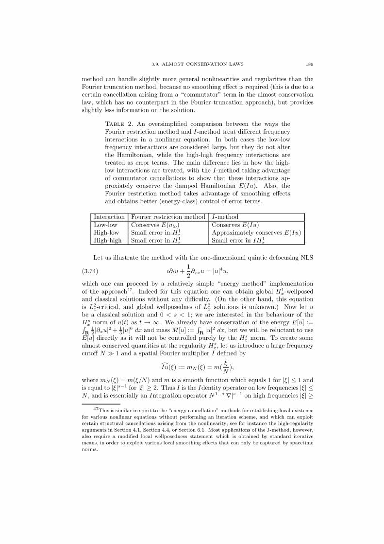
3.9. ALMOST CONSERVATION LAWS 189
method can handle slightly more general nonlinearities and regularities than theFourier truncation method, because no smoothing effect is required (this is due to acertain cancellation arising from a “commutator” term in the almost conservationlaw, which has no counterpart in the Fourier truncation approach), but providesslightly less information on the solution.
Table 2. An oversimplified comparison between the ways theFourier restriction method and I-method treat different frequencyinteractions in a nonlinear equation. In both cases the low-lowfrequency interactions are considered large, but they do not alterthe Hamiltonian, while the high-high frequency interactions aretreated as error terms. The main difference lies in how the high-low interactions are treated, with the I-method taking advantageof commutator cancellations to show that these interactions ap-proxiately conserve the damped Hamiltonian E(Iu). Also, theFourier restriction method takes advantage of smoothing effectsand obtains better (energy-class) control of error terms.
Interaction Fourier restriction method I-methodLow-low Conserves E(ulo) Conserves E(Iu)High-low Small error in H1
x Approximately conserves E(Iu)High-high Small error in H1
x Small error in IH1x
Let us illustrate the method with the one-dimensional quintic defocusing NLS
(3.74) i∂tu+1
2∂xxu = |u|4u,
which one can proceed by a relatively simple “energy method” implementationof the approach47. Indeed for this equation one can obtain global H1
x-wellposedand classical solutions without any difficulty. (On the other hand, this equationis L2
x-critical, and global wellposednes of L2x solutions is unknown.) Now let u
be a classical solution and 0 < s < 1; we are interested in the behaviour of theHsx norm of u(t) as t → ∞. We already have conservation of the energy E[u] :=∫
R
12 |∂xu|2 + 1
3 |u|6 dx and mass M [u] :=∫R|u|2 dx, but we will be reluctant to use
E[u] directly as it will not be controlled purely by the Hsx norm. To create some
almost conserved quantities at the regularity Hsx, let us introduce a large frequency
cutoff N ≫ 1 and a spatial Fourier multiplier I defined by
Iu(ξ) := mN (ξ) = m(ξ
N),
where mN (ξ) = m(ξ/N) and m is a smooth function which equals 1 for |ξ| ≤ 1 andis equal to |ξ|s−1 for |ξ| ≥ 2. Thus I is the Identity operator on low frequencies |ξ| ≤N , and is essentially an Integration operator N1−s|∇|s−1 on high frequencies |ξ| ≥
47This is similar in spirit to the “energy cancellation” methods for establishing local existencefor various nonlinear equations without performing an iteration scheme, and which can exploitcertain structural cancellations arising from the nonlinearity; see for instance the high-regularity
arguments in Section 4.1, Section 4.4, or Section 6.1. Most applications of the I-method, however,also require a modified local wellposedness statement which is obtained by standard iterativemeans, in order to exploit various local smoothing effects that can only be captured by spacetimenorms.

190 3. SEMILINEAR DISPERSIVE EQUATIONS
N ; this explains why this operator is denoted “I”. We now show that the modifiedenergy E[Iu(t)] =
∫R
12 |∂xIu(t)|2 + 1
3 |Iu(t)|6 dx obeys an almost conservation law.
Proposition 3.38 (Almost conservation law). Let s > 1/2. Suppose t is atime such that E[Iu(t)] . 1. Then |∂tE[Iu(t)]| .s N
−1/2.
The exponent 1/2 here might not be best possible. An improvement of theexponent here will lead to a better global wellposedness result for a conclusion, aswill be clear from the remainder of this argument.
Proof. For a general classical field v, we have the identity
∂tE[v(t)] = −2Re
∫
R
∂tv(i∂tv +1
2∂xxv − |v|4v) dx
which can be easily verified by integration by parts; note that this reproves theconservation of energy for (3.74). We now set v := Iu; by applying I to (3.74) wesee that v solves the equation
i∂tv +1
2∂xxv = I(|u|4u)
and hence we have
∂tE[v(t)] = −2Re
∫
R
I∂tu(I(|u|4u) − |Iu|4Iu) dx.
Thus it will suffice to establish the bound
|∫
R
I∂tu(I(|u|4u) − |Iu|4Iu) dx| . N−1/2.
Splitting ∂tu = 12∂xxu− i|u|4u, we can split this further into
(3.75) |∫
R
I∂xxu(I(|u|4u) − |Iu|4Iu) dx| . N−1/2
and
(3.76) |∫
R
I(|u|4u)(I(|u|4u) − |Iu|4Iu) dx| . N−1/2.
We shall just prove the top order estimate (3.75) and leave the lower order estimate(3.76) as an exercise. To avoid technicalities we shall “cheat” somewhat by assumingheuristics such as the fractional Leibnitz rule (A.14) as if they were rigorous; onecan justify all the cheats performed here by Littlewood-Paley theory and othertools of Fourier analysis but we shall not do so here. We integrate one of thepartial derivatives by parts, and observe from the hypothesis E[Iu(t)] . 1 that‖I∂xu‖L2
x. 1. Thus it suffices to show the commutator estimate
‖∂x[I(|u|4u) − |Iu|4Iu]‖L2x
. N−1/2/
We split u = uhi + ulo, where uhi := P>N/100u and ulo := P≤N/100u. We can
then expand |u|4u and |Iu|4Iu into a large number of terms involving five factorsfrom uhi and ulo. There are three types of terms to consider. First consider the“low-low” terms that only involve ulo:
‖∂x[I(|ulo|4ulo) − |Iulo|4Iulo]‖L2x.
Because I is the Identity on low frequencies, we see that both I(|ulo|4ulo) and|Iulo|4Iulo are equal to |ulo|4ulo and so the net contribution of these terms is zero.

3.9. ALMOST CONSERVATION LAWS 191
Next, consider any “high-high” term that involves two or more factors of uhi. Hereis a typical one (we do not attempt to exploit cancellation here):
‖∂xI(uhi2u3lo)‖L2
x.
The operator ∂xI is a pseudodifferential operator of positive order. Applying thefractional Leibnitz rule, we can distribute this operator and end up consideringterms, of which the following is typical:
‖O(|∂xIuhi||uhi||ulo|3‖L2x.
Now from the Gagliardo-Nirenberg inequality and the hypothesis E[Iu(t)] . 1 wehave ‖Iu‖L∞
x. 1, and in particular ‖ulo‖L∞
x. 1. Also we have already remarked
that ‖∂xIuhi‖L2x
. 1, which by an easy Fourier analytic argument (exploiting thehigh frequency nature of uhi and the hypothesis s > 1/2) implies that ‖uhi‖L∞
x.s
N−1/2; see Exercise 3.68. The desired bound then follows from Holder’s inequality.Finally, we must consider “high-low” terms involving only one factor of uhi.
Here we must use48 the cancellation present in (3.75). A typical term to consideris
‖∂x[I(|ulo|4uhi) − |ulo|4Iuhi]‖L2x,
where we have used the fact that Iulo = ulo. The expression in brackets is thecommutator of I and |ulo|4, applied to uhi. Let us write w := |ulo|4. The Fouriertransform of ∂x(I(wuhi) − wIuhi) at ξ can be computed to be
i
∫
R
ξ[m(ξ
N) −m(ξ − ηN)]w(η)uhi(ξ − η) dη.
The integrand vanishes unless |η| . N and |ξ| & N . In such a case, an application
of the mean-value theorem gives the bound ξ(m( ξN ) −m(ξ − ηN)) = O(|η|m((ξ −η)/N)). On the other hand, the expression
∫
R
|η|m((ξ − η)/N)w(η)uhi(ξ − η) dη
is essentially the Fourier transform of (|∇|w)Iuhi. Thus we morally have
∂x[I(|ulo|4uhi) − |ulo|4Iuhi]“ .′′ (|∇|w)Iuhi
in some Fourier sense. Assuming this to be rigorous, we are reduced to establishingthat
‖(|∇|w)Iuhi‖L2x
. N−1/2.
Now we already know that ‖Iuhi‖L∞x
. N−1/2. Also by distributing the derivative|∇| using the fractional Leibnitz rule, we can (morally) replace |∇|w by an expres-sion such as O(||∇|ulo|×|ulo|3). Since we already know that ‖ulo‖L∞
x. ‖Iu‖L∞
x. 1
and ‖|∇|ulo‖L2x
. ‖∇Iu‖L2x
. 1, the claim now follows from Holder’s inequality.
From the above proposition and the continuity method, we conclude that ifE[Iu(0)] = O(1), then in fact E[Iu(t)] = O(1) for all |t| ≪s N
1/2. Thus thequantity E[Iu(t)] is stable for long periods of time. One can now apply scalingarguments and some Fourier analysis to conclude
48An alternative would be to try to average in time and exploit bilinear refinements toStrichartz’ inequality here; this is related to the extra smoothing effect alluded to earlier. However,the approach given in the text demonstrates that one can use the commutator cancellation in theI-method as a substitute for such smoothing effects.
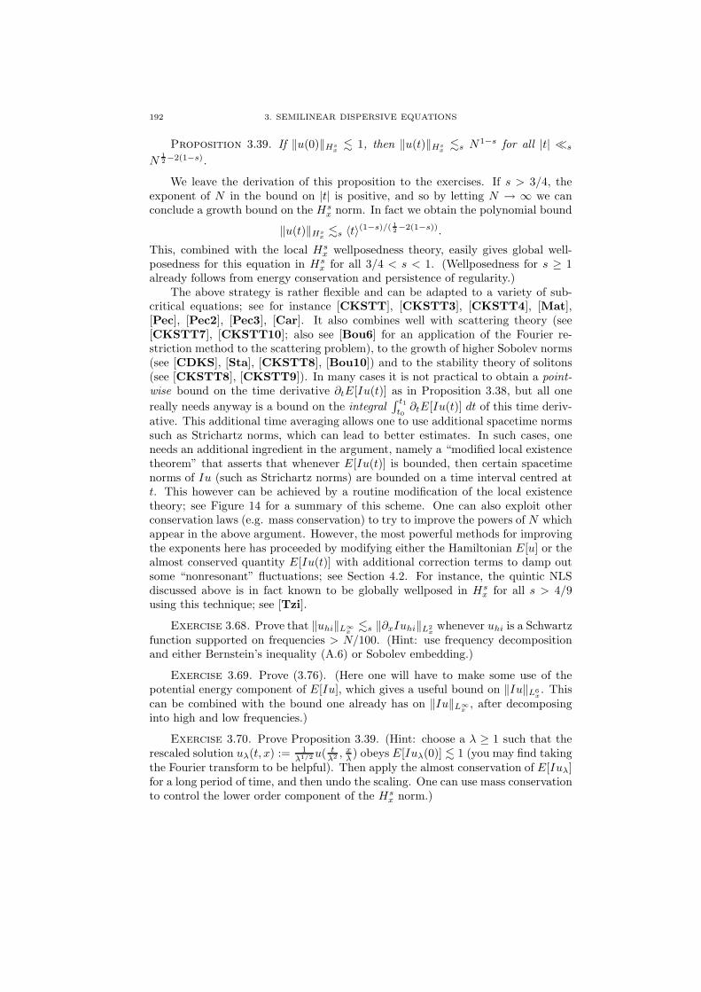
192 3. SEMILINEAR DISPERSIVE EQUATIONS
Proposition 3.39. If ‖u(0)‖Hsx
. 1, then ‖u(t)‖Hsx
.s N1−s for all |t| ≪s
N12−2(1−s).
We leave the derivation of this proposition to the exercises. If s > 3/4, theexponent of N in the bound on |t| is positive, and so by letting N → ∞ we canconclude a growth bound on the Hs
x norm. In fact we obtain the polynomial bound
‖u(t)‖Hsx
.s 〈t〉(1−s)/(12−2(1−s)).
This, combined with the local Hsx wellposedness theory, easily gives global well-
posedness for this equation in Hsx for all 3/4 < s < 1. (Wellposedness for s ≥ 1
already follows from energy conservation and persistence of regularity.)The above strategy is rather flexible and can be adapted to a variety of sub-
critical equations; see for instance [CKSTT], [CKSTT3], [CKSTT4], [Mat],[Pec], [Pec2], [Pec3], [Car]. It also combines well with scattering theory (see[CKSTT7], [CKSTT10]; also see [Bou6] for an application of the Fourier re-striction method to the scattering problem), to the growth of higher Sobolev norms(see [CDKS], [Sta], [CKSTT8], [Bou10]) and to the stability theory of solitons(see [CKSTT8], [CKSTT9]). In many cases it is not practical to obtain a point-wise bound on the time derivative ∂tE[Iu(t)] as in Proposition 3.38, but all one
really needs anyway is a bound on the integral∫ t1t0∂tE[Iu(t)] dt of this time deriv-
ative. This additional time averaging allows one to use additional spacetime normssuch as Strichartz norms, which can lead to better estimates. In such cases, oneneeds an additional ingredient in the argument, namely a “modified local existencetheorem” that asserts that whenever E[Iu(t)] is bounded, then certain spacetimenorms of Iu (such as Strichartz norms) are bounded on a time interval centred att. This however can be achieved by a routine modification of the local existencetheory; see Figure 14 for a summary of this scheme. One can also exploit otherconservation laws (e.g. mass conservation) to try to improve the powers of N whichappear in the above argument. However, the most powerful methods for improvingthe exponents here has proceeded by modifying either the Hamiltonian E[u] or thealmost conserved quantity E[Iu(t)] with additional correction terms to damp outsome “nonresonant” fluctuations; see Section 4.2. For instance, the quintic NLSdiscussed above is in fact known to be globally wellposed in Hs
x for all s > 4/9using this technique; see [Tzi].
Exercise 3.68. Prove that ‖uhi‖L∞x
.s ‖∂xIuhi‖L2x
whenever uhi is a Schwartzfunction supported on frequencies > N/100. (Hint: use frequency decompositionand either Bernstein’s inequality (A.6) or Sobolev embedding.)
Exercise 3.69. Prove (3.76). (Here one will have to make some use of thepotential energy component of E[Iu], which gives a useful bound on ‖Iu‖L6
x. This
can be combined with the bound one already has on ‖Iu‖L∞x
, after decomposinginto high and low frequencies.)
Exercise 3.70. Prove Proposition 3.39. (Hint: choose a λ ≥ 1 such that therescaled solution uλ(t, x) := 1
λ1/2u(tλ2 ,
xλ) obeys E[Iuλ(0)] . 1 (you may find taking
the Fourier transform to be helpful). Then apply the almost conservation of E[Iuλ]for a long period of time, and then undo the scaling. One can use mass conservationto control the lower order component of the Hs
x norm.)

3.9. ALMOST CONSERVATION LAWS 193
on [t , t ]0 1
local theorymodified
Iu(t ) in H0
1
0E(I(u(t )) bounded 0E(I(u(t )) bounded 0E(I(u(t )) bounded
su(t ) in H
su(t ) in H
[almost conservationlaw]
on [t , t ]local theorymodified
21
Iu(t ) in H1
1Iu(t ) in H
1
2
[rescale]
0 2
[undorescaling]
[almost conservationlaw]
Figure 14. The general scheme of the I-method; compare withFigure 7. Of course, one would usually iterate the method for morethan the two time steps indicated here. Apart from the rescalingand the presence of the I operator, one new feature is that the(modified) local theory plays a quantitative role rather than merelya qualitative one, as this theory is necessary to control the errorterms in the almost conservation law. However, it is importantthat the local theory does not impact the main term in that law,otherwise the H1
x norm of Iu(t) could increase exponentially witheach time step.

194 3. SEMILINEAR DISPERSIVE EQUATIONS
log M
log || P u ||M H1
N
upper bound on u
upper bound on Iu
Figure 15. A log-log plot of the energy of the Littlewood-Paleypieces PMu(0) of u(0) as a function of M , when u(0) is assumedto only lie in Hs
x for some s < 1. Note the infinite energy athigh frequencies. The operator I smooths out the energy at highfrequencies, giving Iu(0) a large but finite energy. A rescaling isthen needed to make the energy bounded by 1.
3.9. ALMOST CONSERVATION LAWS 195
log M
log || P u ||M H1
N
upper bound on u
upper bound on Iu
Figure 16. A log-log plot of the energy of the Littlewood-Paleypieces PMu(t) of u(t) as a function of M , for some late time t (apower of N). The almost conservation law keeps the energy of Iubounded but large (because of the scaling), but we do not excludethe possibility that energy has been moved around in the frequencyranges M . N . Thus at each time t, the high frequencies stillevolve in a somewhat linear (non-interacting) fashion, but the lowand medium frequencies may share their energy with each other.As time progresses, more and more frequencies could mix theirenergy, potentially leading to a polynomial growth in the Hs
x norm.


CHAPTER A
Appendix: tools from harmonic analysis
Every action of our lives touches on some chord that will vibratein eternity. (Sean O’Casey)
The nonlinear evolution equations studied here can be profitably analyzed byviewing these equations as describing the oscillation and interaction between low,medium, and high frequencies. To make this type of analysis rigorous, we of courseneed the notation and tools of harmonic analysis, and in particular the Fouriertransform and Littlewood-Paley theory; the purpose of this appendix is to reviewthat material. This is only an outline of the material; for a more thorough intro-duction to these tools from a PDE-oriented perspective, see [Tay], [Tay2].
It is convenient to work in the Schwartz class Sx(Rd). One particularly im-portant operation on Schwartz functions (and hence on their dual) is the (spatial)
Fourier transform f 7→ f , defined for f ∈ Sx(Rd) by the formula1
f(ξ) :=
∫
Rd
f(x)e−ix·ξ dx.
As is well known, the Fourier transform f 7→ f is a Frechet space automorphismon the Schwartz space Sx(Rd), with the inversion formula
f(x) =1
(2π)d
∫
Rd
f(ξ)eix·ξ dξ.
Thus every Schwartz function can be formally viewed as a superposition of planewaves eix·ξ. We also have the fundamental Plancherel identity
∫
Rd
|f(x)|2 dx =1
(2π)d
∫
Rd
|f(ξ)|2 dξ
as well as the closely related Parseval identity2
(A.1)
∫
Rd
f(x)g(x) dx =1
(2π)d
∫
Rd
f(ξ)g(ξ) dξ.
The Fourier transform enjoys many symmetry properties, several of which we listin Table 1. Of particular importance to PDE is the relation lies in the fact that it
1It is customary to omit the factor of 2π from the Fourier exponent in PDE, in order tosimplify the Fourier multipliers associated to any given PDE; of course, this factor then surfacesin the Fourier inverion formula. In any event, the factors of 2π make only a negligible impact onthe theory, so much so that some authors choose to abuse notation slightly, and simply omit allfactors of 2π in their arguments.
2Some authors reverse the attribution of these two identities, which are easily shown tobe equivalent. Strictly speaking, Parseval’s original identity was for Fourier series, whereasPlancherel’s theorem concerned Fourier integrals.
329
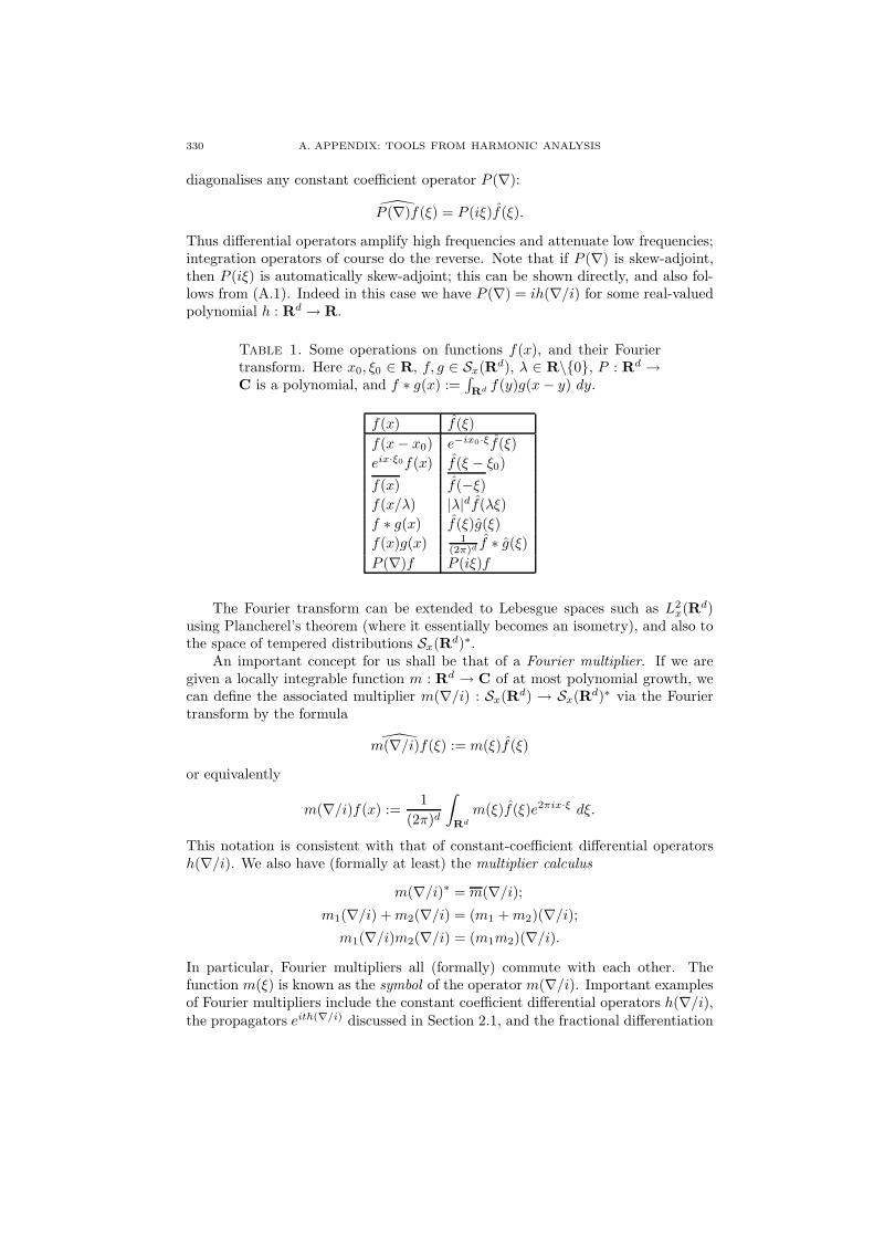
330 A. APPENDIX: TOOLS FROM HARMONIC ANALYSIS
diagonalises any constant coefficient operator P (∇):
P (∇)f (ξ) = P (iξ)f(ξ).
Thus differential operators amplify high frequencies and attenuate low frequencies;integration operators of course do the reverse. Note that if P (∇) is skew-adjoint,then P (iξ) is automatically skew-adjoint; this can be shown directly, and also fol-lows from (A.1). Indeed in this case we have P (∇) = ih(∇/i) for some real-valuedpolynomial h : Rd → R.
Table 1. Some operations on functions f(x), and their Fouriertransform. Here x0, ξ0 ∈ R, f, g ∈ Sx(Rd), λ ∈ R\0, P : Rd →C is a polynomial, and f ∗ g(x) :=
∫Rd f(y)g(x− y) dy.
f(x) f(ξ)
f(x− x0) e−ix0·ξf(ξ)
eix·ξ0f(x) f(ξ − ξ0)
f(x) f(−ξ)f(x/λ) |λ|df(λξ)
f ∗ g(x) f(ξ)g(ξ)
f(x)g(x) 1(2π)d f ∗ g(ξ)
P (∇)f P (iξ)f
The Fourier transform can be extended to Lebesgue spaces such as L2x(R
d)using Plancherel’s theorem (where it essentially becomes an isometry), and also tothe space of tempered distributions Sx(Rd)∗.
An important concept for us shall be that of a Fourier multiplier. If we aregiven a locally integrable function m : Rd → C of at most polynomial growth, wecan define the associated multiplier m(∇/i) : Sx(Rd) → Sx(Rd)∗ via the Fouriertransform by the formula
m(∇/i)f(ξ) := m(ξ)f (ξ)
or equivalently
m(∇/i)f(x) :=1
(2π)d
∫
Rd
m(ξ)f(ξ)e2πix·ξ dξ.
This notation is consistent with that of constant-coefficient differential operatorsh(∇/i). We also have (formally at least) the multiplier calculus
m(∇/i)∗ = m(∇/i);m1(∇/i) +m2(∇/i) = (m1 +m2)(∇/i);m1(∇/i)m2(∇/i) = (m1m2)(∇/i).
In particular, Fourier multipliers all (formally) commute with each other. Thefunction m(ξ) is known as the symbol of the operator m(∇/i). Important examplesof Fourier multipliers include the constant coefficient differential operators h(∇/i),the propagators eith(∇/i) discussed in Section 2.1, and the fractional differentiation

A. APPENDIX: TOOLS FROM HARMONIC ANALYSIS 331
and integration operators |∇|α and 〈∇〉α defined3 for all α ∈ R, with symbols |ξ|αand 〈ξ〉α respectively. This in turn leads to the Sobolev spaces W s,p
x (Rd) and the
homogeneous Sobolev spaces W s,px (Rd), defined for s ∈ R and 1 < p < ∞ as the
closure of the Schwartz functions under their respective norms
‖f‖W s,px (Rd) := ‖〈∇〉sf‖Lp
x(Rd)
and
‖f‖W s,px (Rd) := ‖|∇|sf‖Lp
x(Rd).
Thus these spaces generalise the Lebesgue spaces, which correspond to the casess = 0. In the special case p = 2, we writeHs
x and Hsx forW s,2
x and W s,2x respectively.
From Plancherel’s theorem we observe that
‖f‖Hsx(Rd) =
1
(2π)d/2‖〈ξ〉sf‖L2
ξ(Rd)
and similarly
‖f‖Hsx(Rd) =
1
(2π)d/2‖|ξ|sf‖L2
ξ(Rd).
Using Calderon-Zygmund theory (see e.g. [Stei]), one can show the identities
‖f‖W s,px (Rd) ∼s,p,d ‖f‖W s−1,p
x (Rd) + ‖∇f‖W s−1,px (Rd);
‖f‖W s,px (Rd) ∼s,p,d ‖∇f‖W s−1,p
x (Rd)
for any 1 < p < ∞ and s ∈ R. Iterating the above inequalities, we obtain thatthese Sobolev norms are equivalent (up to constants) to their classical counterparts,thus
‖f‖Wk,px (Rd) ∼k,p,d
k∑
j=0
‖∇jf‖Lpx(Rd)
and
‖f‖Wk,px (Rd) ∼k,p,d ‖∇kf‖Lp
x(Rd).
We will not define Sobolev spaces at p = 1 or p = ∞ to avoid the technicalitiesassociated with endpoint Calderon-Zygmund theory.
Another important class of Fourier multipliers are the Littlewood-Paley multi-pliers. Let us fix a real-valued radially symmetric bump function ϕ(ξ) adapted tothe ball ξ ∈ Rd : |ξ| ≤ 2 which equals 1 on the ball ξ ∈ Rd : |ξ| ≤ 1; theexact choice of bump function turns out in practice to not be important4. Definea dyadic number to be any number N ∈ 2Z of the form N = 2j where j ∈ Z isan integer; any sum over the dummy variable N or M is understood to be over
3For α ≤ −d, the operator |∇|α is only defined for Schwartz functions which obey enoughmoment conditions that their Fourier transform vanishes to high order at the origin. As we shallnever use integration operators of such low order, we shall ignore this technicality.
4In the classical Littlewood-Paley theory (see e.g. [Stei]), one uses the harmonic extension or
heat extension, which would correspond to the (non-compactly-supported) choices ϕ(ξ) := e−|ξ|
or ϕ(ξ) := e−|ξ|2 respectively. However in the modern theory it has turned out to be moreconvenient to use compactly supported bump functions (but see Section 6.4).

332 A. APPENDIX: TOOLS FROM HARMONIC ANALYSIS
dyadic numbers unless otherwise specified. For each dyadic number N , we definethe Fourier multipliers
P≤Nf(ξ) := ϕ(ξ/N)f(ξ)
P>Nf(ξ) := (1 − ϕ(ξ/N))f (ξ)
PNf(ξ) := (ϕ(ξ/N) − ϕ(2ξ/N))f(ξ).
We similarly define P<N and P≥N . Thus PN , P≤N , P>N are smoothed out projec-tions to the regions |ξ| ∼ N , |ξ| ≤ 2N , |ξ| > N respectively. Note in particular thetelescoping identities
P≤Nf =∑
M≤NPMf ; P>Nf =
∑
M>N
PMf ; f =∑
M
PMf
for all Schwartz f , where M ranges over dyadic numbers. We also define
PM<·≤N := P≤N − P≤M =∑
M<N ′≤NPN ′
whenever M ≤ N are dyadic numbers. Similarly define PM≤·≤N , etc.Littlewood-Paley projections are extremely handy in the rigorous study of PDE,
because they separate (in a quantitative manner) the rough (high-frequency, oscil-lating, low regularity) components of a solution from the smooth (low-frequency,slowly varying, high regularity) components, thus clarifying the nature of variouscomponents of the equation, such as derivatives and various nonlinear interactionsof the solution with itself. The following heuristics are quite useful (see Figure 1).
Principle A.1 (Uncertainty principle). Let N be a dyadic number, and let fbe a function on Rd.
• (Low frequencies) If f has Fourier transform supported on frequencies ofmagnitude |ξ| . N (e.g. if f = P≤Ng for some g), then f should be ap-proximately constant on spatial balls of radius c/N for small c, and ∇sfshould be “dominated” by Nsf for any s ≥ 0. (Thus localisation at fre-quency scales N forces a spatial uncertainty of 1/N ; this is a manifestationof the Heisenberg uncertainty principle |δx · δξ| & 1.)
• (High frequencies) If f has Fourier transform supported on frequenciesof magnitude |ξ| & N (e.g. if f = P≥Ng for some g), then f shouldhave approximate mean zero5 on balls of radius C/N for large C, and∇−sf should be “dominated” by N−sf for any s ≥ 0. (Thus exclusion offrequencies at scales N and below forces spatial oscillation at scale 1/N .)
• (Medium frequencies) If f has Fourier transform supported on frequenciesof magnitude |ξ| ∼ N (e.g. if f = PNg for some g), then both of the aboveheuristics should apply, and ∇sf should be “comparable” to Nsf for bothpositive and negative s.
We now present some concrete estimates that make the above intuition rigorous.One easily verifies that P≤N is a convolution operator, in fact
P≤Nf(x) =1
(2π)d
∫
Rd
ϕ(y)f(x+y
N) dy.
5In fact, we expect higher moments to vanish as well, so that f should be approximatelyorthogonal to any bounded degree polynomials on these balls.

A. APPENDIX: TOOLS FROM HARMONIC ANALYSIS 333
NP g
P<N
f
P h>N
x
x
1/N
x
Figure 1. The uncertainty principle. The low-frequency functionP<Nf has frequencies less than N and is thus essentially constantat spatial scales ≪ 1/N . The high-frequency function P>Nh hasfrequencies greater than N and thus oscillates (with mean essen-tially zero) at spatial scales ≫ 1/N . The medium-frequency func-tion PNg behaves in both fashions simultaneously.
Since ϕ is rapidly decreasing and has unit mass, one thus can think of P≤N as anaveraging operator that “blurs” f by a spatial scale of O(1/N), and localises f infrequency to the ball of radius O(N), which is consistent with Principle A.1. Fromthis identity one can easily verify (using Young’s inequality, and the commutativityof all Fourier multipliers) that the above Littlewood-Paley operators are bounded(uniformly in N or M) on every Lebesgue space Lpx(R
d) with 1 ≤ p ≤ ∞, as well
as every Sobolev space W s,px (Rd), W s,p
x (Rd) for s ∈ R and 1 < p < ∞. Further-more, they obey the following easily verified (see Exercise A.1) and extremely usefulBernstein inequalities for Rd with s ≥ 0 and 1 ≤ p ≤ q ≤ ∞:
‖P≥Nf‖Lpx(Rd) .p,s,d N
−s‖|∇|sP≥Nf‖Lpx(Rd)(A.2)
‖P≤N |∇|sf‖Lpx(Rd) .p,s,d N
s‖P≤Nf‖Lpx(Rd)(A.3)
‖PN |∇|±sf‖Lpx(Rd) ∼p,s,d N±s‖PNf‖Lp
x(Rd)(A.4)
‖P≤Nf‖Lqx(Rd) .p,q,d N
dp− d
q ‖P≤Nf‖Lpx(Rd)(A.5)
‖PNf‖Lqx(Rd) .p,q,d N
dp− d
q ‖PNf‖Lpx(Rd).(A.6)
Thus when the frequency is localised, one can upgrade low Lebesgue integrability tohigh Lebesgue integrability, at the cost of some powers of N ; when the frequency

334 A. APPENDIX: TOOLS FROM HARMONIC ANALYSIS
N is very low, this cost is in fact a gain, and it becomes quite desirable to useBernstein’s inequality whenever the opportunity arises. These estimates can beverified by computation of the distributional kernel of PN and P≤N , and theirderivatives, followed by Young’s inequality. A deeper estimate, requiring someCalderon-Zygmund theory, is the Littlewood-Paley inequality
(A.7) ‖f‖Lpx(Rd) ∼p,d ‖(
∑
N
|PNf |2)1/2‖Lpx(Rd);
see for instance [Stei2]. In a similar spirit, from Plancherel’s theorem we have theestimate
(A.8) ‖f‖Hsx(Rd) ∼s,d (
∑
N
N2s‖PNf‖2L2
x(Rd))1/2
and
(A.9) ‖f‖Hsx(Rd) ∼s,d ‖P≤1f‖L2
x(Rd) + (∑
N>1
N2s‖PNf‖2L2
x(Rd))1/2
As a sample application of these estimates, let us present
Lemma A.2 (Hardy’s inequality). If 0 ≤ s < d/2 then
‖|x|−sf‖L2x(Rd) .s,d ‖f‖Hs
x(Rd).
Proof. The case s = 0 is trivial, so suppose 0 < s < d/2. Using (A.8) itsuffices to show that∫
Rd
|f(x)|2|x|2s dx .s,d
∑
N
N2s‖PNf‖2L2
x(Rd).
We subdivide the left-hand side into dyadic shells and estimate∫
Rd
|f(x)|2|x|2s dx .s,d
∑
R
R−2s
∫
|x|≤R|f(x)|2 dx
where R ranges over dyadic numbers. Using Littlewood-Paley decomposition andthe triangle inequality, we have
(
∫
|x|≤R|f(x)|2 dx)1/2 ≤
∑
N
(
∫
|x|≤R|PNf(x)|2 dx)1/2.
On the one hand we have the trivial estimate
(
∫
|x|≤R|PNf(x)|2 dx)1/2 ≤ ‖PNf‖L2
x(Rd)
while on the other hand by Bernstein (A.6) and Holder we have
(
∫
|x|≤R|PNf(x)|2 dx)1/2 .d R
d/2‖PNf‖L∞x (Rd) .d (NR)d/2‖PNf‖L2
x(Rd).
Combining all these estimates together, we reduce to establishing that∑
R
R−2s(∑
N
min(1, (NR)d/2)‖PNf‖L2x(Rd))
2 .s,d
∑
N
N2s‖PNf‖2L2
x(Rd).
Writing cN := Ns‖PNf‖L2x(Rd), this becomes
‖∑
N
min((NR)−s, (NR)d/2−s)cN‖l2R(2Z) .s,d ‖cN‖l2N (2Z)

A. APPENDIX: TOOLS FROM HARMONIC ANALYSIS 335
where 2Z is the space of dyadic numbers. But since 0 < s < d/2, the kernelmin(M−s,Md/2−s) is absolutely convergent over dyadic numbers. The claim nowfollows from Young’s inequality (or Minkowski’s inequality, or Schur’s test).
In a similar spirit we have
Proposition A.3 (Gagliardo-Nirenberg inequality). Let 1 < p < q ≤ ∞ ands > 0 be such that
1
q=
1
p− θs
d
for some 0 < θ < 1. Then for any u ∈ W s,px (Rd) we have
‖u‖Lqx(Rd) .d,p,q,s ‖u‖1−θ
Lpx(Rd)
‖u‖θW s,p
x (Rd).
In the special case q = ∞, we conclude in particular (by the usual approximationby Schwartz function argument) that u is in fact continuous (so it lies in C0
x(Rd)).
Proof. We may of course assume that u is non-zero. The inequality is invari-ant under homogeneity u(x) 7→ λu(x) and scaling u(x) 7→ u(x/λ) for any λ > 0.Using these invariances we may normalise ‖u‖Lp
x(Rd) = ‖u‖W s,px (Rd) = 1.
The next step is the Littlewood-Paley decomposition u =∑N PNu, where N
ranges over dyadic numbers. From the triangle inequality followed by Bernstein’sinequality we have
‖u‖Lqx(Rd) ≤
∑
N
‖PNu‖Lqx(Rd)
.d,p,q
∑
N
Ndp− d
q ‖PNu‖Lpx(Rd)
=∑
N
Nθs‖PNu‖Lpx(Rd)
On the other hand, from (A.4) and the boundedness of PN have
‖PNu‖Lpx(Rd) .d,p ‖u‖Lp
x(Rd) = 1; ‖PNu‖Lpx(Rd) .d,p,s N
−s‖|∇|su‖Lpx(Rd) = N−s.
Inserting this into the previous estimate we obtain
‖u‖Lqx(Rd) .d,p,s
∑
N
Nθsmin(1, N−s) .θ,s 1
and the claim follows (note that θ is determined by d, p, q, s).
Closely related to the above two inequalities is the Hardy-Littlewood-Sobolevtheorem of fractional integration, which asserts that
(A.10) ‖f ∗ 1
|x|α ‖Lqx(Rd) .p,q,d ‖f‖Lp
x(Rd)
whenever 1 < p < q < ∞ and 0 < α < d obey the scaling condition 1p = 1
q + d−αd .
This implies the homogeneous Sobolev embedding
(A.11) ‖f‖Lqx(Rd) .p,q,d ‖f‖W s,p
x (Rd)
whenever 1 < p < q <∞ and s > 0 obey the scaling condition 1p = 1
q + sd , which in
turn implies the inhomogeneous Sobolev embedding
(A.12) ‖f‖Lqx(Rd) .p,q,s,d ‖f‖W s,p
x (Rd)
336 A. APPENDIX: TOOLS FROM HARMONIC ANALYSIS
whenever 1 < p < q < ∞ and s > 0 is such that 1p ≤ 1
q + sd . We leave the proofs
as exercises. Note that the non-endpoint case 1p <
1q + s
d of (A.12) already follows
from Proposition A.3, and we also have an extension to the q = ∞ case, namely
‖f‖C0x(Rd) = ‖f‖L∞
x (Rd) .p,s,d ‖f‖W s,px (Rd)
whenever 1 < p <∞ and s > 0 is such that 1p <
sd . In particular we have
(A.13) ‖f‖C0x(Rd) = ‖f‖L∞
x (Rd) .s,d ‖f‖Hsx(Rd)
when s > n/2.The Sobolev embedding theorem (A.11) is sharp in the following sense: if f
is a rescaled bump function, say f = Nαψ(Nx) for some ψ ∈ Sx(Rd) and someN > 0 and α ∈ R, then one can verify that ‖f‖Lq
x(Rd) ∼ψ,q,d N−d/qNα and
‖f‖W s,px (Rd) ∼ψ,s,p,d NsN−d/pNα, and so from the scaling condition 1
p = 1q + s
d
we see that both sides of (A.11) are comparable. A useful fact is that these bumpfunctions are in some sense the only way in which both sides of Sobolev embeddingestimate can be close to comparable. Indeed, we have
Proposition A.4 (Inverse Sobolev theorem). Let 1 < p < q < ∞, s > 0, and0 < η ≤ 1.
• If 1p = 1
q + sd and f is such that ‖f‖W s,p
x (Rd) . 1 and ‖f‖Lqx(Rd) & η,
then there exists a dyadic number N and a position x0 ∈ Rd such that|PNf(x0)| ∼p,q,d,η Nd/q, and furthermore
(
∫
|x−x0|≤C/N|PNf(x)|r dx)1/r ∼p,q,d,η N
dq −d
r
for all 1 ≤ r ≤ ∞ and some large constant C = C(p, q, d, η) > 0.• If 1
p <1q + s
d and f is such that ‖f‖W s,px (Rd) . 1 and ‖f‖Lq
x(Rd) & η, then
there exists a dyadic number N ∼p,q,s,d,η 1 and a position x0 ∈ Rd suchthat |PNf(x0)| ∼p,q,s,d,η 1, and furthermore
(
∫
|x−x0|≤C|PNf(x)|r dx)1/r ∼p,q,s,d,η 1
for all 1 ≤ r ≤ ∞ and some large constant C = C(p, q, s, d, η) > 0.
More informally, in order for (A.11) to be close to sharp, f must contain alarge normalised bump function at some position x0 and some frequency N (andwavelength 1/N); in order for (A.12) to be sharp, we have a similar conclusionbut with the additional information that the frequency N is comparable to 1. Toput it another way, in order to come within a constant to saturating the Sobolevembedding theorem, the function must concentrate a significant portion of its W s,p
x
“energy” in a ball. (See also Lemma B.4, which essentially asserts that if one comeswithin an epsilon of the best constant in a Sobolev embedding type theorem, thenone must concentrate nearly all of one’s energy in a ball.) The implicit constantshere can be made more explicit, for instance the dependence on η is polynomial,but we will not need such quantitative bounds here. See [BG] for an applicationof these types of theorems to nonlinear wave equations.
A. APPENDIX: TOOLS FROM HARMONIC ANALYSIS 337
Proof. We will just prove the (easier) second half of the theorem here, andleave the first to Exercise A.7. We have
η . ‖f‖Lqx(Rd) .
∑
N
‖PNf‖Lqx(Rd).
Now from (A.6), (A.4), and the hypothesis ‖f‖W s,px (Rd) . 1 we have
‖PNf‖Lqx(Rd) .p,q,d,s N
dp−d
q ‖PNf‖Lpx(Rd) .p,q,d,s N
dp− d
q min(1, N−s).
The hypotheses on p, q, s ensure that∑
N Ndp− d
q min(1, N−s) is geometrically de-creasing as N → 0 or N → ∞ and is thus convergent. We conclude that there existsN ∼p,q,s,d,η 1 such that ‖PNf‖Lq
x(Rd) &p,q,s,d,η 1. Since ‖PNf‖Lpx(Rd) .p,q,s,d,η 1,
we conclude from Holder’s inequality that ‖PNf‖L∞x (Rd) &p,q,s,d,η 1. Thus there
exists x0 ∈ Rd such that |PNf(x0)| &p,q,s,d,η 1. Writing PNf = PN/4<·<4NPNf ,we can express PNf(x0) as the inner product of PNf with a rapidly decreasing ap-proximation to the identity centred at x0. Since we also have ‖PNf‖Lp
x(Rd) .d,p,s 1,an easy application of Holder’s inequality then gives
∫
|x−x0|≤C|PNf(x)| dx &p,q,s,d,η 1
for some large C = C(p, q, s, d, η). On the other hand, from Bernstein’s inequalitywe have ‖PNf‖L∞
x (Rd) .d,p,s 1. The claim then follows from Holder’s inequalityagain.
We have seen how Littlewood-Paley technology is useful for understanding lin-ear operations such as fractional integration. It is also invaluable in understandingnonlinear operations, such as multiplication (f, g) 7→ fg or composition u 7→ F (u)for various explicit functions F . Both of these operations arise constantly in non-linear PDE, and there are two very useful heuristics that can be used to understandthem:
Principle A.5 (Fractional Leibnitz rule). Let f, g be functions on Rd, andlet Dα be some sort of differential or pseudodifferential operator of positive orderα > 0.
• (High-low interactions) If f has significantly higher frequency than g (e.g.if f = PNF and g = P<N/8G for some F,G), or is “rougher” than g (e.g.f = ∇u and g = u for some u) then fg will have comparable frequencyto f , and we expect Dα(fg) ≈ (Dαf)g. In a similar spirit we expectPN (fg) ≈ (PNf)g.
• (Low-high interactions) If g has significantly higher frequency or is rougherthan f , then we expect fg to have comparable frequency to g. We alsoexpect Dα(fg) ≈ f(Dαg), and PN (fg) ≈ f(PNg).
• (High-high interactions) If f and g have comparable frequency (e.g. f =PNF and g = PNG for some F,G) then fg should have frequency com-parable or lower than f , and we expect Dα(fg) / (Dαf)g ≈ f(Dαg).
• (Full Leibnitz rule) With no frequency assumptions on f and g, we expect
(A.14) Dα(fg) ≈ f(Dαg) + (Dαf)g.
Principle A.6 (Fractional chain rule). Let u be a function on Rd, and letF : R → R be a “reasonably smooth” function (e.g. F (u) = |u|p−1u). Then we

338 A. APPENDIX: TOOLS FROM HARMONIC ANALYSIS
have the fractional chain rule
(A.15) Dα(F (u)) ≈ F ′(u)Dαu
for any differential operator Dα of positive order α > 0, as well as the Littlewood-Paley variants
P<N (F (u)) ≈ F (P<Nu)
and
(A.16) PN (F (u)) ≈ F ′(P<Nu)PNu.
If F is complex instead of real, we have to replace F ′(u)Dαu by Fz(u)Dαu+FzDαu,
and similarly for (A.16).
Observe that when Dα is a differential operator of order k, then the heuristics(A.14), (A.15) are accurate to top order in k (i.e. ignoring any terms which onlydifferentiate f, g, u k − 1 or fewer times). Indeed, the above two principles areinstances of a more general principle:
Principle A.7 (Top order terms dominate). When distributing derivatives, thedominant terms are usually6 the terms in which all the derivatives fall on a singlefactor; if the factors have unequal degrees of smoothness, the dominant term willbe the one in which all the derivatives fall on the roughest (or highest frequency)factor.
A complete and rigorous treatment of these heuristics (sometimes called parad-ifferential calculus) is beyond the scope of this text, and we refer the reader to[Tay2]. We will however give some representative instances of these heuristics inaction.
Lemma A.8 (Product lemma). If s ≥ 0, then we have the estimate
(A.17) ‖fg‖Hsx(Rd) .s,d ‖f‖Hs
x(Rd)‖g‖L∞x (Rd) + ‖f‖L∞
x (Rd)‖g‖Hsx(Rd)
for all f, g ∈ Hsx(R
d) ∩L∞x (Rd). In particular, if s > d/2, we see from the Sobolev
embedding (A.13) that we have the algebra property
(A.18) ‖fg‖Hsx(Rd) .s,d ‖f‖Hs
x(Rd)‖g‖Hsx(Rd).
Observe that (A.17) heuristically follows from (A.14), since that latter heuristicsuggests that
〈∇〉s(fg) ≈ (〈∇〉sf)g + f(〈∇〉sg)and the claim then (non-rigorously) follows by taking L2
x norms of both sides andthen using the triangle and Holder inequalities.
Proof. The basic strategy with these multilinear estimates is to decomposeusing the Littlewood-Paley decomposition, eliminate any terms that are obviouslyzero (because of impossible frequency interactions), estimate each remaining com-ponent using the Bernstein and Holder inequalities, and then sum. One shouldalways try to apply Bernstein on the lowest frequency possible, as this gives themost efficient estimates. In some cases one needs to apply Cauchy-Schwarz toconclude the summation.
6In some cases, there is a special cancellation which allows one to treat the dominant termsdirectly. In such cases one often then has to look at the next term in the “Taylor expansion” inwhich all but one derivative falls on one term, and the remaining derivative falls on another. Thisphenomenon underlies a number of commutator estimates, such as those discussed in Section 3.9.

A. APPENDIX: TOOLS FROM HARMONIC ANALYSIS 339
The claim is trivial for s = 0, so assume s > 0. From (A.9) we have
(A.19) ‖fg‖Hsx(Rd) .s,d ‖P≤1(fg)‖L2
x(Rd) + (∑
N>1
N2s‖PN (fg)‖2L2
x(Rd))1/2.
We shall just bound the latter term, and leave the former term to the exercises.We split7
‖PN(fg)‖L2x(Rd) . ‖PN((P<N/8f)g)‖L2
x(Rd) +∑
M>N/8
‖PN((PMf)g‖L2x(Rd).
For the first term, observe from Fourier analysis that we may freely replace g byPN/8<·<8Ng, and so by Holder’s inequality
‖PN ((P<N/8f)g)‖L2x(Rd) .d ‖(P<N/8f)PN/8<·<8Ng‖L2
x(Rd)
.d ‖f‖L∞x (Rd)
∑
M∼N‖PMg‖L2
x(Rd)
and so the total contribution of this term to (A.19) is Os,d(‖f‖L∞x (Rd)‖g‖Hs
x(Rd)).For the second term, we simply bound
∑
M>N/8
‖PN ((PMf)g)‖L2x(Rd) .d
∑
M>N/8
‖(PMf)g‖L2x(Rd)
.d ‖g‖L∞x (Rd)
∑
M&N
‖PMf‖L2x(Rd)
.d,s ‖g‖L∞x (Rd)
∑
M&N
M−s‖PMf‖Hsx(Rd)
and so by Cauchy-Schwarz
(Ns∑
M>N/8
‖PN((PMf)g)‖L2x(Rd))
2 .d,s ‖g‖2L∞
x (Rd)
∑
M&N
NsM−s‖PMf‖2Hs
x(Rd).
Summing this in N (and using the hypothesis s > 0) we see that the total contri-bution of this term is Os,d(‖f‖Hs
x(Rd)‖g‖L∞x (Rd)), and we are done.
Lemma A.9 (Schauder estimate). Let V be a finite-dimensional normed vectorspace, let f ∈ Hs
x(Rd → V ) ∩ L∞
x (Rd → V ) for some s ≥ 0. Let k be the firstinteger greater than s, and let F ∈ Ckloc(V → V ) be such that F (0) = 0. ThenF (f) ∈ Hs
x(Rd → V ) as well, with a bound of the form
‖F (f)‖Hsx(Rd) .F,‖f‖
L∞x (Rd)
,V,s,d ‖f‖Hsx(Rd).
Note that when F is real analytic, one can deduce this from Lemma A.8; butthe argument below is rather robust and extends to rougher types of function F .For instance, when s ≤ 1 the argument in fact only requires Lipschitz control on F .The reader should heuristically verify that Lemma A.9 follows immediately fromPrinciple A.6 in much the same way that Lemma A.8 follows from Principle A.5.
7This is a basic example of a paraproduct decomposition, in which a genuine product suchas fg is split as the sum of paraproducts (combinations of products of Littlewood-Paley pieces).
Paraproducts are usually easier to estimate analytically, especially if derivatives are involved,because they specifically identify which of the factors is high frequency and which is low frequency,allowing one to use the flexible estimates (A.2)-(A.6) in a manner adapted to the paraproduct athand, instead of relying only on “one-size-fits-all” tools such as Sobolev embedding.

340 A. APPENDIX: TOOLS FROM HARMONIC ANALYSIS
The reader may also wish to verify the s = 1 case of this estimate by hand (withF Lipschitz) in order to get some sense of why this type of estimate should hold.
Proof. The strategy to prove nonlinear is related, though not quite the sameas, that used to prove multilinear estimates. Basically, one should try to splitF (f) using Taylor expansion into a rough error, which one estimates crudely, anda smooth main term, which one estimates using information about its derivatives.Again, one uses tools such as Holder, Bernstein, and Cauchy-Schwarz to estimatethe terms that appear.
Let us write A := ‖f‖L∞x (Rd). Since F is Ckloc and F (0) = 0, we see that
|F (f)| .F,A,V |f |. This already establishes the claim when s = 0. Applying (A.9),it thus suffices to show that
(∑
N>1
N2s‖PNF (f)‖2L2
x(Rd))1/2 .F,A,V,s ‖f‖Hs
x(Rd).
for all s > 0.We first throw away a “rough” portion of F (f) in PNF (f). Fix N, s, and split
f = P<Nf +P≥Nf . Note that f and P<Nf are both bounded by OV,d(A). Now Fis Ckloc, hence Lipschitz on the ball of radius OV,d(A), hence we have
F (f) = F (P<Nf) +OF,A,V,d(|P≥Nf |),and thus
‖PNF (f)‖L2x(Rd) .F,A,V,d ‖PNF (P<Nf)‖L2
x(Rd) + ‖P≥Nf‖L2x(Rd).
To control the latter term, observe from the triangle inequality and Cauchy-Schwarzthat
N2s‖P≥Nf‖2L2
x(Rd) .s
∑
N ′≥N(N ′)sNs‖PN ′f‖2
L2x(Rd)
and summing this in N and using (A.9) we see that this term is acceptable. Thusit remains to show that
(∑
N>1
N2s‖PNF (P<Nf)‖2L2
x(Rd))1/2 .F,A,V,s ‖f‖Hs
x(Rd).
We will exploit the smoothness of P<Nf and F by using (A.4) to estimate
(A.20) ‖PNF (P<Nf)‖L2x(Rd) .d,k N
−k‖∇kF (P<Nf)‖L2x(Rd).
Applying the chain rule repeatedly, and noting that all derivatives of F are boundedon the ball of radius OV,d(A), we obtain the pointwise estimate
|∇kF (P<Nf)| .F,A,V,d,k supk1+...+kr=k
|∇k1(P<Nf)| . . . |∇kr (P<Nf)|
where r ranges over 1, . . . , k and k1, . . . , kr range over non-negative integers thatadd up to k. We split this up further using Littlewood-Paley decomposition as
|∇kF (P<Nf)| .F,A,V,d,k supk1+...+kr=k
∑
1≤N1,...,Nr<N
|∇k1(PN1f)| . . . |∇kr (PNrf)|
where we adopt the convention that PN := PN when N > 1 and P1 := P≤1. Bygiving up a factor of r! = Ok(1) we may take N1 ≤ N2 . . . ≤ Nr. where k1, . . . , krrange over all positive integers that add up to k. Now from (A.4) we have
‖∇ki(PNif)‖L∞x (Rd) .d,k N
ki
i ‖f‖L∞x (Rd) .d,k,A N
ki

A. APPENDIX: TOOLS FROM HARMONIC ANALYSIS 341
for i = 1, . . . , r − 1, and similarly
‖∇kr (PNrf)‖L∞x (Rd) .d,k N
krr ‖PNrf‖L2
x(Rd)
and hence we have
‖∇kF (P<Nf)‖L2x(Rd) .F,A,V,d,k
supk1+...+kr=k
∑
1≤N1≤...≤Nr<N
Nk11 . . . Nkr
r ‖PNrf‖L2x(Rd).
Performing the sum in N1, then N2, then finally Nr−1, and rewriting N ′ := Nr, weobtain
‖∇kF (P<Nf)‖L2x(Rd) .F,A,V,d,k
∑
1≤N ′<N
(N ′)k‖PN ′f‖L2x(Rd).
By Cauchy-Schwarz and (A.20) we conclude
‖PNF (P<Nf)‖2L2
x(Rd) .F,A,V,d,k
∑
1≤N ′<N
(N ′)kN−k‖PN ′f‖2L2
x(Rd).
Summing this in N and using (A.9) we see that this term is acceptable (note thatk depends only on s, so the dependence on k is not a concern).
In computations involving momentum, one often encounters expressions suchas
∫Rd u∇v dx or
∫Rd u(x)(
x|x| · ∇v). The following lemma is useful for controlling
these quantities.
Lemma A.10 (Momentum estimate). Let u, v ∈ S(Rd) for some d ≥ 3, and letK be a kernel on Rd which is smooth away from the origin, and obeys the estimates
|K(x)| .d 1; |∇K(x)| .d |x|−1
away from the origin. (For instance, we could have K(x) ≡ 1, or K(x) ≡ xj
|x| for
some j = 1, . . . , d.) Then we have
|∫
Rd
u(x)K(x)∇v(x) dx| .d ‖u‖Hsx(Rd)‖v‖H1−s
x (Rd)
for all 0 ≤ s ≤ 1 (in particular, the estimate is true for s = 1/2).
Intuitively speaking, the justification for this lemma is that we can integrateby parts “1/2 times” to move half of the derivative from v onto u, ignoring themild symbol K in between. By standard limiting arguments we may now extend
the bilinear form (u, v) 7→∫Rd u(x)K(x)∇v(x) dx to all u, v ∈ H
1/2x (Rd), dropping
the hypothesis that u, v is Schwartz.
Proof. A standard regularisation argument (replacing K by K ∗ φε for someapproximation to the identity φε, and then letting ε → 0, taking advantage of thehypothesis that u, v are Schwartz) allows us to assume that K is smooth on all ofRd (including the origin), provided of course that our estimates are uniform in K.By real or complex interpolation it will suffice to establish the estimates
|∫
Rd
u(x)K(x)∇v(x) dx| .d ‖u‖L2x(Rd)‖v‖H1
x(Rd)
and
|∫
Rd
u(x)K(x)∇v(x) dx| .d ‖u‖H1x(Rd)‖v‖L2
x(Rd).
342 A. APPENDIX: TOOLS FROM HARMONIC ANALYSIS
The first estimate is immediate from Holder’s inequality (estimating u, ∇v in L2x and
K in L∞x ). For the second estimate, we integrate by parts (again taking advantage
of the hypothesis that u, v are Schwartz) and use the triangle inequality to estimate
|∫
Rd
u(x)K(x)∇v(x) dx| ≤ |∫
Rd
(∇u)(x)K(x)v(x) dx|+|∫
Rd
u(x)(∇K)(x)v(x) dx|.
The first term can be estimated by Holder’s inequality as before. The second termcan be estimated by Cauchy-Schwarz (placing v in L2
x) followed by Lemma A.2(with s = 1 and d ≥ 3), and we are done.
Exercise A.1. Prove (A.2)-(A.6). (Hint: for each of the estimates, use Fourieranalysis to write the expression in the left-hand norm as the convolution of theexpression in the right-hand norm with some explicit kernel, and then use Young’sinequality.) Discuss why these estimates are consistent with Principle A.1.
Exercise A.2. Deduce (A.13) directly from the Fourier inversion formula andCauchy-Schwarz, and show that it fails at the endpoint s = d/2.
Exercise A.3 (Lorentz characterisation of Lpx). [KTao] Let f ∈ Lpx(Rd) for
some 1 < p < ∞. Show that one can decompose f =∑k ckχk, where k ranges
over the integers, χk is a function bounded in magnitude by 1 and supported on aset of measure at most 2k, and ck are a sequence of non-negative reals such that(∑
k 2k|ck|p)1/p ∼p ‖f‖Lpx(Rd). (Hint: let f∗(x) := infα : ||f | > α| < x be the
(left-continuous) nondecreasing rearrangement of |f |. Set ck to equal f∗(2k−1), andckχk be the portion of f where f∗(2k) < |f(x)| ≤ f∗(2k−1).)
Exercise A.4 (Dual Lorentz characterisation of Lqx). Let f ∈ Lqx(Rd) for some
1 < q <∞. Show that
‖f‖Lqx(Rd) ∼q sup
Ek
(∑
k
2k(1−q)|∫
Ek
f(x) dx|q)1/q
where for each k, Ek ranges over all bounded open sets of measure 2k. (Hint: use the
nondecreasing rearrangement again. Show that supEk|∫Ekf(x) dx| ∼q
∫ 2k
0f∗(t) dt,
and then decompose the interval [0, 2k] dyadically.)
Exercise A.5. Use Exercises A.3, A.4 to prove (A.10). (Hint: first establishthe estimate
|∫
Ek′
χk ∗1
|x|α | .d,α min(2d−α
d k2k′
, 2d−α
d k′2k)
for all k, k′, where Ek′ and χk are as in the preceding exercises.) Deduce (A.11)and (A.12) as a consequence.
Exercise A.6 (Lorentz refinement of Sobolev embedding). For 1 < p, q <∞,define the Lorentz norm
‖f‖Lq,px (Rd) := sup
Ek
(∑
k
2k(pq −p)|
∫
Ek
f(x) dx|p)1/p
where Ek is as in Exercise A.4. By repeating the proof of Exercise A.5, refine theestimate (A.11) to
‖f‖Lqx(Rd) .p,q,d ‖f‖Lq,p
x (Rd) .p,q,d ‖f‖W s,px (Rd)
under the same hypotheses on p, q, d, s.

A. APPENDIX: TOOLS FROM HARMONIC ANALYSIS 343
Exercise A.7. Prove the first half of Proposition A.4. (Hint: first use ExerciseA.6 to show that |
∫Ekf(x) dx| ∼p,q,d,η 2k(1−1/q) for some k ∈ Z and some set Ek
of measure 2k. Then perform a Littlewood-Paley decomposition of f to concludethat ‖PNf‖L∞
x (Rd) &p,q,d,η 2k(1−1/q) for some N ∼p,q,d,η 2−k/d.)
Exercise A.8 (Relationship between Sobolev and isoperimetric inequalities).Let d > 1. Prove the endpoint Sobolev estimate
||f(x)| ≥ λ| .d
‖|∇f |‖d/(d−1)
L1x(Rd)
λd/(d−1)
for any λ > 0 and f ∈ Sx(Rd). (Hint: estimate |f | pointwise by |∇f | ∗ 1|x|d−1 . Let
E := |f(x)| ≥ λ and obtain a pointwise bound for 1E ∗ 1|x|d−1 . Alternatively,
use induction on d to establish the slightly stronger estimate ‖f‖Ld/(d−1)(Rd) .d
‖|∇f |‖L1x(Rd).) If Ω ⊂ Rd is a bounded domain with smooth boundary, deduce the
isoperimetric inequality
|∂Ω| &d |Ω|(d−1)/d
where |∂Ω| is the surface area of Ω. (Hint: set f to be a smoothed out versionof 1Ω.) It is well known that among all domains with fixed volume, the ball hasthe smallest surface area; comment on how this is compatible with the heuristicssupporting Proposition A.4.
Exercise A.9. Give a heuristic justification of Principle A.5 using the Fouriertransform and the elementary estimate 〈ξ + η〉s .s 〈ξ〉s + 〈η〉s for all ξ, η ∈ Rd.
Exercise A.10. Complete the proof of Lemma A.8.
Exercise A.11. Generalise Lemma A.8 by replacing Hsx with W s,p
x for some1 < p <∞, and replacing the condition s > d/2 with s > d/p. (Hint: you will needthe Littlewood-Paley estimate (A.7).)
Exercise A.12. Let the assumptions and notation be as in Lemma A.9, butsuppose that F lies in Ck+1
loc rather than just in Ckloc. Establish the Lipschitzestimate
‖F (f) − F (g)‖Hsx(Rd) .F,‖f‖
L∞x (Rd)
,‖g‖L∞
x (Rd),V,s,d ‖f − g‖Hs
x(Rd).
(Hint: One could repeat the proof of Lemma A.9, but a slicker proof is to use the
fundamental theorem of calculus to write F (f)−F (g) =∫ 1
0DF ((1−θ)f+θg) ·(f−
g) dθ, where DF is the differential of F , and then apply Lemma A.9 and LemmaA.8.)
Exercise A.13 (Fractional chain rule). [CWein] Let p > 1, and let F ∈C1
loc(C → C) be a function of pth power type, in the sense that F (z) = O(|z|p) and∇F (z) = Op(|z|p−1). Let 0 ≤ s < 1 and 1 < q < r <∞ obey the scaling conditiondq = dp
r − (p− 1)s. Show that
‖PNF (f)‖W s,qx (Rd) .d,p,q,r,s ‖f‖pW s,r
x (Rd)
for all f ∈ W s,rx (Rd) and N > 0. (Note that this is rather easy to justify heuris-
tically from Principle A.6.) If furthermore p > 2, and F is C2loc with ∇2F (z) =
Op(|z|p−2), establish the stronger estimate
‖PN(F (f)−F (g))‖W s,qx (Rd) .d,p,q,r,s (‖f‖W s,r
x (Rd)+‖g‖W s,rx (Rd))
p−1‖f−g‖W s,rx (Rd)
344 A. APPENDIX: TOOLS FROM HARMONIC ANALYSIS
for all f, g ∈ W s,rx (Rd) and N > 0. It is possible to remove the PN projections,
and obtain the stronger estimates
‖F (f)‖W s,qx (Rd) .d,p,q,r,s ‖f‖pW s,r
x (Rd)
and
‖F (f) − F (g)‖W s,qx (Rd) .d,p,q,r,s (‖f‖W s,r
x (Rd) + ‖g‖W s,rx (Rd))
p−1‖f − g‖W s,rx (Rd)
but this is quite challenging (requiring tools such as the Littlewood-Paley squarefunction inequality and the Fefferman-Stein vector-valued maximal inequality) andbeyond the scope of this text.
Exercise A.14. If I is an interval in R and 2 ≤ q, r < ∞, establish theinequality
‖u‖LqtL
rx(I×Rd) .d,q,r (
∑
N
‖PNu‖2Lq
tLrx(I×Rd))
1/2.
(Hint: use (A.7). To interchange the norm and square function, first consider theextreme cases q, r = 2,∞ and then interpolate, for instance using the complexmethod.)
Exercise A.15. If I is a bounded interval in R, and u, ∂tu ∈ L2t (I), use
elementary arguments to obtain a localised Gagliardo-Nirenberg inequality
‖u‖L∞t (I) . ‖u‖1/2
L2t(I)
‖∂tu‖1/2
L2t(I)
and the Poincare inequality
‖u− 1
I
∫
I
u‖L2t(I)
. |I|‖∂tu‖L2t(I)
.
Exercise A.16 (Hardy inequality revisited). Let u ∈ Sx(Rd). Use integrationby parts to establish the identity
∫
Rd
|x|α|x · ∇u(x)|2 dx =(d+ α)2
4
∫
Rd
|x|α|u(x)|2 dx
+
∫
Rd
|x|α|x · ∇u(x) − d+ α
2u(x)|2 dx
for any α > −d, and use this to establish another proof of Hardy’s inequality in thecase s = 1.
Exercise A.17. Give another proof of Lemma A.10 which does not use inter-polation, but relies instead on Littlewood-Paley decomposition. (Hint: you mayneed to decompose K smoothly into dyadic pieces also and use arguments similarto those used to prove Lemma A.2.) The techniques of interpolation and of dyadicdecomposition are closely related; the latter tends to be messier but more flexible.
Exercise A.18 (Localisation ofHsx functions). Let u ∈ Hs
x(Rd) for some s ≥ 0,
and let ψ ∈ Sx(Rd). Show that for any R ≥ 1 we have
‖u(x)ψ(x
R)‖Hs
x(Rd) .s,d,ψ ‖u‖Hsx(Rd).
This very useful fact allows one to smoothly localise functions in Hsx to large balls,
uniformly in the size of the ball. (Hint: prove this for s a positive integer byinduction first, and then use interpolation. You may find the Hardy or Sobolev

A. APPENDIX: TOOLS FROM HARMONIC ANALYSIS 345
inequalities to be useful. An alternate approach is to perform a Fourier decompo-sition of ψ and work entirely in frequency space.) Similarly, if u ∈ H1
x(Rd) and
d ≥ 3, establish the bound
‖u(x)ψ(x
R)‖H1
x(Rd) .ψ,d ‖u‖H1x(Rd).
Exercise A.19 (Radial Sobolev inequality). Let d ≥ 3, and let u be a Schwartzfunction on Rd. Establish the inequality
‖|x| d2−1|u|‖L∞
x (Rd) .d ‖u‖H1x(Rd)
for all x ∈ Rd, as well as the variant
‖|x|s|u|‖L∞x (Rd) .d,s ‖u‖H1
x(Rd)
for all d2 − 1 ≤ s ≤ d−1
2 . (Hint: if |x| = R, truncate u smoothly to the region|x| ∼ R using Exercise A.18, use polar coordinates, and use the Gagliardo-Nirenberginequality.)
Exercise A.20. If f is spherically symmetric, show that one can take x0 =Os,p,q,d,η(1/N) in Proposition A.4; thus Sobolev embedding is only sharp near theorigin (using the natural length scale associated to the frequency). (Hint: if x0 istoo far away from the origin, use the symmetry to find a large number of disjointballs, each of which absorb a significant portion of energy.)
Exercise A.21 (Littlewood-Paley characterisation of Holder regularity). Let0 < α < 1 and 1 ≤ p ≤ ∞. If f ∈ Sx(Rd), we define the Holder norm ‖f‖Λp
α(Rd)
by the formula
‖f‖Λpα(Rd) := ‖f‖Lp
x(Rd) + suph∈Rd:0<|h|≤1
‖fh − f‖Lpx(Rd)
|h|α
where fh(x) = f(x+ h) is the translate of f by h. Show that
‖f‖Λpα(Rd) ∼p,α,d ‖f‖Lp
x(Rd) + supN≥1
Nα‖PNf‖Lpx(Rd).
(Hint: to control the latter by the former, express PNf as an average of functionsof the form fh − f . To control the former by the latter, obtain two bounds forthe Lpx norm of PNf
h − PNf , using the triangle inequality in the high frequencycase N & |h|−1 and the fundamental theorem of calculus in the low frequency caseN . |h|−1.) The latter expression is essentially an example of a Besov norm, whichoften functions as a substitute for the Sobolev norm which is a little more tech-nically convenient in several PDE applications, particularly those in which one isconcerned about controlling interactions between high and low frequencies. Con-clude in particular that
‖f‖Wα−ε,px (Rd) .p,α,d,ε ‖f‖Λp
α(Rd) .p,α,d ‖f‖Wα,px (Rd)
for any ε > 0; thus Holder norms are “within an epsilon” of their Sobolev counter-parts.
Exercise A.22 (Morrey-Sobolev inequality). If 0 < α < 1 and d < p ≤ d1−α ,
show that
‖f‖Λ∞α (Rd) .p,α,d ‖f‖W 1,p
x (Rd)

346 A. APPENDIX: TOOLS FROM HARMONIC ANALYSIS
for all f ∈ Sx(Rd), where Λ∞α was defined in the previous exercise. This reflects a
general principle, that if there is some “surplus” regularity in the Sobolev embed-ding theorem that causes one to go past L∞
x , this additional regularity will thenmanifest itself as Holder continuity, and one can again recover endpoint estimates.
Exercise A.23 (Hodge decomposition). Let φ : Hsx(R
d → Rd) be a vectorfield. Show that one has a unique decomposition φ = φcf +φdf into a curl-free vectorfield φcf ∈ Hs
x(Rd → Rd) and a divergence-free vector field φdf ∈ Hs
x(Rd → Rd),
thus curlφcf = ∇ ∧ φcf = 0 and divφdf = ∇ · φdf = 0 in the sense of distributions.Verify the identities φcf = ∆−1∇(∇ · φ) and φdf = ∆−1∇¬(∇ ∧ φ). If s = 0, showthat φcf and φdf are orthogonal. (You may either use the Fourier transform, ortake divergences and curls of the decomposition φ = φcf + φdf to solve for φcf andφdf .)
Exercise A.24 (Div-curl lemma). Let φ, ψ : L2x(R
d → Rd) be vector fieldssuch that divφ = 0 and curlψ = 0. Show that
∫Rd φ · ψ = 0, and also that
φ · ψ ∈ H−d/2x (Rd); this is a simple example of a div-curl lemma, that exploits
a certain “high-high” frequency cancellation between divergence-free and curl-freevector fields, and forms a key component of the theory of compensated compactness ;see for instance [CLMS]. (Note that Holder’s inequality would place φ · ψ in L1
x,
which is not enough for Sobolev embedding to place into H−d/2x 3. To prove the
lemma, use Hodge theory to write φ and ψ as the curl and gradient of a H1x 2-form
and scalar field respectively, then use Littlewood-Paley decomposition.)
Exercise A.25 (Sobolev trace lemma). Let f ∈ Sx(Rd) for d ≥ 2, and viewRd−1 ≡ Rd−1 × 0 as a subset of Rd in the usual manner. Show that
‖f‖Hsx(Rd−1) .d,s ‖f‖Hs+1/2
x (Rd)
and‖f‖Hs
x(Rd−1) .d,s ‖f‖Hs+1/2x (Rd)
for all s > 0. (This can be done from the Fourier transform; it is also worthwhile totry to prove this from Littlewood-Paley theory, following the heuristics in PrincipleA.1.) Show that these estimates fail when s = 0, and also that the loss of 1/2 aderivative cannot be reduced. One can of course generalise this lemma to othersubsets of Rd of various codimension, and other Sobolev spaces, but we shall notdo so here.
Exercise A.26 (Agmon division lemma). Let f ∈ Sx(R) be such that f(0) = 0.Show that ‖f(x)/x‖Hs−1
x (R) .s ‖f‖Hsx(R) for all s > 1/2. (Hint: write f(x)/x =
∫ 1
0f ′(tx) dt, then take Fourier transforms.)

Bibliography
[AF] M. Ablowitz, A. Fokas, The inverse scattering transform for the Benjamin-Ono equation, apivot for multidimensional problems, Stud. Appl. Math. 68 (1983), 1–10.
[Ale] A. D. Alexandrov, Uniqueness theorems for surfaces in the large, V. Vestnik LeningradUniv. Mat. Mekh. Astronom. 13 (1958), 5–8; Amer. Math. Soc. Transl. Ser 2. 21 (1962),412–416.
[Arn] V.I. Arnold, Mathematical methods in classical mechanics (3rd edn). Nauka, Moscow, 1974.English translation, 2nd edn, Springer-Verlag, Berlin, 1989.
[BZS] J. Baez, Z. Zhou, I.E. Segal, The global Goursat problem and scattering for nonlinear waveequations, J. Func. Anal. 93 (1990), 239–296.
[BG] H. Bahouri, P. Gerard, High frequency approximation of solutions to critical nonlinear waveequations, Amer. J. Math. 121 (1999), 131–175.
[BS] H. Bahouri, J. Shatah, Decay estimates for the critical semilinear wave equation, Ann. Inst.H. Poincare Anal. Non Lineaire 15 (1998),783–789.
[Bea] M. Beals, Self-Spreading and strength of Singularities for solutions to semilinear waveequations, Annals of Math 118 (1983), 187–214.
[BB] M. Beals, M. Bezard, Low regularity local solutions for field equations, Comm. Partial Dif-ferential Equations 21 (1996), 79–124.
[BT] I. Bejenaru, T. Tao, Sharp well-posedness and ill-posedness results for a quadratic non-linearSchrodinger equation, to appear, J. Func. Anal.
[Ben] T. Benjamin, Internal waves of permanent form in fluids of great depth, J. Fluid Mech. 29
(1967), 559–562.[BKPSV] B. Birnir, C. Kenig, G. Ponce, N. Svanstedt, L. Vega, On the ill-posedness of the IVP
for the generalized Korteweg-de Vries and nonlinear Schrodinger equations, J. London Math.Soc. 53 (1996), 551–559.
[BPS] B. Birnir, G. Ponce, N. Svanstedt, The local ill-posedness of the modified KdV equation,
Ann. Inst. H. Poincare Anal. Non Lineaire 13 (1996), 529–535.[BC] P. Blue, J. Colliander, Global well-posedness in Sobolev space implies global existence for
weighted L2 initial data for L2-critical NLS, preprint.[BSmi] J. Bona, R. Smith, The initial-value problem for the Korteweg-de Vries equation, Philos.
Trans. Royal Soc. London Series A 278 (1975), 555–601.[Bou] J. Bourgain, Fourier restriction phenomena for certain lattice subsets and applications to
nonlinear evolution equations, Parts I, II, Geometric and Funct. Anal. 3 (1993), 107–156,209–262.
[Bou2] J. Bourgain, Approximation of solutions of the cubic nonlinear Schrodinger equations byfinite-dimensional equations and nonsqueezing properties, Int. Math. Res. Notices, 1994, no.2, (1994), 79–90.
[Bou3] J. Bourgain, Aspects of longtime behaviour of solutions of nonlinear Hamiltonian evolutionequations, Geom. Func. Anal. 5 (1995), 105–140.
[Bou4] J. Bourgain, Periodic nonlinear Schrodinger equations and invariant measures, Comm.Math. Phys. 166 (1995), 1–26.
[Bou5] J. Bourgain, Periodic Korteweg de Vries equation with measures as initial data, SelectaMath. (N.S.) 3 (1997), 115–159.
[Bou6] J. Bourgain. Scattering in the energy space and below for 3D NLS, Jour. D’Anal. Math.,75 (1998), 267–297.
[Bou7] J. Bourgain, Global well-posedness of defocusing 3D critical NLS in the radial case, J.Amer. Math. Soc. 12 (1999), 145-171.
363

364 BIBLIOGRAPHY
[Bou8] J. Bourgain, Refinements of Strichartz Inequality and Applications to 2d-NLS With Crit-ical Nonlinearity, Inter. Math. Res. Not., (1998), p. 253–284.
[Bou9] J. Bourgain, New global well-posedness results for non-linear Schrodinger equations, AMSPublications, 1999.
[Bou10] J. Bourgain, A remark on normal forms and the ‘I-Method’ for periodic NLS, J. Anal.Math. 94 (2004), 125–157.
[BK] J. Bourgain, V. Kaloshin, On diffusion in high-dimensional Hamiltonian systems, J. Func.Anal. 229 (2005), 1–61.
[BW] J. Bourgain, W. Wang, Construction of blowup solutions for the nonlinear Schrodingerequation with critical non-linearity, Dedicated to Ennio De Giorgi. Ann. Scuola Norm. Sup.Pisa Cl. Sci. (4) 25 (1997), no. 1-2, 197-215.
[BC] J. P. Boyd, G. Chen, Weakly nonlinear wavepackets in the Korteweg-de Vries equation: TheKdV/NLS connection, Math. Comput. Simulation 56 (2001), 317–328.
[BGT] N. Burq, P. Gerard, N. Tzvetkov, An instability property of the nonlinear Schrodingerequation on Sd, Math. Res. Lett. 9 (2002), 323–335.
[BP] N. Burq, F. Planchon, On well-posedness for the Benjamin-Ono equation, preprint.[Car] X. Carvajal, Sharp global well-posedness for a higher order Schrodinger equation, preprint.[Caz] T. Cazenave, An introduction to nonlinear Schrodinger equations, Textos de Metodos
Matematicos 26, Instituto de Matematica UFRJ, 1996.
[Caz2] T. Cazenave, Semilinear Schrodinger equations, Courant Lecture Notes in Mathematics,10. New York University, Courant Institute of Mathematical Sciences, AMS, 2003.
[CL] T. Cazenave, Orbital stability of standing waves for some nonlinear Schrodinger equations,Comm. Math. Phys. 68 (1979), 209–243.
[CSS] T. Cazenave, J. Shatah, A.S. Tahvildar-Zadeh, Harmonic maps of the hyperbolic space anddevelopment of singularities in wave maps and Yang-Mills fields, Ann. Inst. H. Poincare Phys.Theor.68 (1998), 315-349.
[CWeis] T. Cazenave, F.B. Weissler, Some remarks on the nonlinear Schrodinger equation in thecritical case, Nonlinear semigroups, Partial Differential Equations and Attractors, LectureNotes in Math. 1394 (1989), 18–29.
[CWeis2] T. Cazenave, F.B. Weissler, Critical nonlinear Schrodinger Equation, Non. Anal. TMA,14 (1990), 807–836.
[CWY] S.Y.A. Chang, L. Wang, P. Yang, Regularity of Harmonic Maps, Comm. Pure. Appl.Math. 52 (1999), 1099–1111.
[Chi] H. Chihara, Local existence for semilinar Schrodinger equations, Math. Japon. 42 (1995),35–52.
[CCT] M. Christ, J. Colliander, T. Tao, Asymptotics, frequency modulation, and low-regularityillposedness of canonical defocussing equations, Amer. J. Math. 125 (2003), 1235–1293.
[CCT2] M. Christ, J. Colliander, T. Tao, Ill-posedness for nonlinear Schrodinger and wave equa-tions, to appear, Annales IHP.
[CCT3] M. Christ, J. Colliander, T. Tao, Instability of the periodic nonlinear Schrodinger equa-tion, preprint.
[CKis] M. Christ, A. Kiselev, Maximal operators associated to filtrations, J. Funct. Anal. 179
(2001).[CWein] M. Christ, M. Weinstein, Dispersion of small amplitude solutions of the generalized
Korteweg-de Vries equation, J. Funct. Anal. 100 (1991), 87–109.[Chr] D. Christodoulou, Global solutions of nonlinear hyperbolic equations for small initial data,
Comm. Pure Appl. Math, 39 (1986), 267–282.[CKla] D. Christodoulou, S. Klainerman, Asymptotic properties of linear field equations in
Minkowski space, Comm. Pure Appl. Math. (1990), 137–199.[CT] D. Christodoulou, A. Tahvildar-Zadeh, On the regularity of spherically symmetric wave
maps, Comm. Pure Appl. Math, 46 (1993), 1041–1091.[CT2] D. Christodoulou, A. Tahvildar-Zadeh, On the asymptotic behavior of a spherically sym-
metric wave map, Duke Math. J. 71 (1993), 31–69.[CLMS] R. Coifman, P.L. Lions, Y. Meyer, S. Semmes, Compensated compactness and Hardy
spaces, J. Math. Pure Appl. 72 (1993), 247–286.[Col] J.D. Cole, On a quasi-linear parabolic equation occurring in aerodynamics, Quart. Appl.
Math. 9 (1951), 225–236.
BIBLIOGRAPHY 365
[CDKS] J. Colliander, J. Delort, C. Kenig, G. Staffilani, Bilinear Estimates and applications to2D NLS, Trans. Amer. Math. Soc. 353 (2001), 3307–3325.
[CKSTT] J. Colliander, M. Keel, G. Staffilani, H. Takaoka, T. Tao, Global well-posedness forKdV in Sobolev spaces of negative index, Electron. J. Diff. Eq. 2001 (2001) No 26, 1–7.
[CKSTT2] J. Colliander, M. Keel, G. Staffilani, H. Takaoka, T. Tao, Sharp global well-posednessfor KdV and modified KdV on R and T, J. Amer. Math. Soc. 16 (2003), 705–749.
[CKSTT3] J. Colliander, M. Keel, G. Staffilani, H. Takaoka, T. Tao, Multilinear estimates forperiodic KdV equations, and applications, preprint 2001, J. Funct. Anal. 211 (2004), 173–218.
[CKSTT4] J. Colliander, M. Keel, G. Staffilani, H. Takaoka, T. Tao, Global well-posedness forSchrodinger equations with derivative, Siam J. Math. 33 (2001), 649–669.
[CKSTT5] J. Colliander, M. Keel, G. Staffilani, H. Takaoka, T. Tao, A refined global well-posedness for the Schrodinger equations with derivative, SIAM J. Math. Anal. 34 (2002),64–86.
[CKSTT6] J. Colliander, M. Keel, G. Staffilani, H. Takaoka, T. Tao, Almost conservation lawsand global rough solutions to a nonlinear Schrodinger equation, Math Res. Lett. 9 (2002),5-6, 659–682.
[CKSTT7] J. Colliander, M. Keel, G. Staffilani, H. Takaoka, T. Tao, Existence globale et diffu-sion pour l’equation de Schrodinger nonlineaire repulsive cubique sur R3 en dessous l’espace
d’energie , Journees “Equations aux Derivees Partielles” (Forges-les-Eaux, 2002), Exp. No.X, 14, 2002.
[CKSTT8] J. Colliander, M. Keel, G. Staffilani, H. Takaoka, T. Tao, Polynomial upper boundsfor the orbital instability of the 1D cubic NLS below the energy norm, Discrete Contin. Dyn.Syst. 9 (2003), 31–54.
[CKSTT9] J. Colliander, M. Keel, G. Staffilani, H. Takaoka, T. Tao, Polynomial growth andorbital instability bounds for L2-subcritical NLS below the energy norm, Commun. Pure Appl.2 (2003), 33–50.
[CKSTT10] J. Colliander, M. Keel, G. Staffilani, H. Takaoka, T. Tao, Scattering for the 3D cubicNLS below the energy norm, Comm. Pure Appl. Math. 57 (2004), 987–1014.
[CKSTT11] J. Colliander, M. Keel, G. Staffilani, H. Takaoka, T. Tao, Global well-posedness andscattering in the energy space for the critical nonlinear Schrodinger equation in R3, to appear,Annals Math.
[CKSTT12] J. Colliander, M. Keel, G. Staffilani, H. Takaoka, T. Tao, Symplectic nonsqueezing ofthe KdV flow , to appear, Acta Math.
[CKSTT13] J. Colliander, M. Keel, G. Staffilani, H. Takaoka, T. Tao, Growth of higher Sobolevnorms for a periodic nonlinear Schrodinger equation, preprint.
[CST] J. Colliander, G. Staffilani, H. Takaoka, Global well-posedness of the KdV equation belowL2, Math Res. Letters 6 (1999), 755-778.
[Cof] C.V. Coffman, Uniqueness of the ground state solution for ∆u−u+u3 = 0 and a variationalcharacterization of other solutions, Arch. Rat. Mech. Anal. 46 (1972), 81–95.
[CS] P. Constantin, J.C. Saut, Effets regularisants locaux pour des equations disperives generales,C. R. Acad. Sci. Paris. Ser. I. Math. 304 (1987), 407–410.
[DG] P. D’Ancona, V. Georgiev, On the continuity of the solution operator of the wave mapssystem, Comm. Pure Appl. Math. 57 (2004), 357–383.
[EL] J. Eells, L. Lemaire, A report on harmonic maps, Bull. London Math. Soc. 10 (1978), no.1, 1–68.
[EL2] J. Eells, L. Lemaire, Another report on harmonic maps, Bull. London Math. Soc. 20 (1988),no. 5, 385–524.
[ES] J. Eells, H. Sampson, Harmonic mappings of Riemannian manifolds, Amer. J. Math. 86
(1964), 109–160.[Eva] C. Evans, Partial Differential Equations, Graduate Studies in Mathematics 19, American
Mathematical Society, 1998.[FW] D. Fang, C. Wang, Some Remarks on Strichartz Estimates for Homogeneous Wave Equa-
tion, preprint.[Fos] D. Foschi, Inhomogeneous Strichartz estimates, Jour. Hyperbolic Diff. Eqs 2, No. 1 (2005)
1–24.[FK] D. Foschi, S. Klainerman, Bilinear space-time estimates for homogeneous wave equations,
Ann. Sci. de l’ENS, 33 no.2 (2000).[Fri] A. Friere, Wave maps to compact Lie groups, preprint.

366 BIBLIOGRAPHY
[FPT] G. Furioli, F. Planchon, E. Terraneo, Unconditional well-posedness for semi-linearSchrodinger equations in Hs, Harmonic analysis at Mount Holyoke, (South Hadley, MA,2001), 147–156.
[FT] G. Furioli, E. Terraneo, Besov spaces and unconditional well-posedness for the nonlinear
Schrodinger equation in Hs,Comm. in Contemp. Math. 5 (2003), 349–367.[GLS] V. Georgiev, H. Lindblad, C. D. Sogge, Weighted Strichartz estimates and global existence
for semilinear wave equations, Amer. J. Math. 119 (1997) 1291–1319.[GNN] B. Gidas, N.W. Ni, L. Nirenberg, Symmetry of positive solutions of nonlinear elliptic
equations in Rn, Mathematical analysis and applications, Part A, pp. 369–402, Adv. in Math.
Suppl. Stud., 7a, Academic Press, New York-London, 1981.[Gin] J. Ginibre, Le probleme de Cauchy pour des EDP semi-lineaires periodiques en variables
d’espace (d’apres Bourgain), Seminaire Bourbaki 1994/1995, Asterisque 237 (1996), Exp.796, 163–187.
[GO] J. Ginibre, T. Ozawa, Long range scattering for nonlinear Schrodinger and Hartree equa-tions in space dimension n >= 2, Comm. Math. Phys. 151 (1993) 619–645.
[GSV] J. Ginibre, A. Soffer, G. Velo, The global Cauchy problem for the critical non-linear waveequation, J. Funct. Anal. 110 (1982), 96–130.
[GTV] J. Ginibre, Y. Tsutsumi, G. Velo, Existence and uniqueness of solutions for the generalizedKorteweg de Vries equation, Math. Z. 203 (1990) 9–36.
[GV] J. Ginibre, G. Velo, Smoothing Properties and Retarded Estimates for Some DispersiveEvolution Equations, Comm. Math. Phys., 123 (1989) , 535–573.
[GV2] J. Ginibre, G. Velo, Generalized Strichartz Inequalities for the Wave Equation, Jour. Func.Anal., 133 (1995), 50–68.
[GV3] J. Ginibre, G. Velo, Scattering theory in the energy space for a class of nonlinearSchrodinger equations, J. Math. Pure. Appl. 64 (1985), 363–401.
[GV4] J. Ginibre, G. Velo, The global Cauchy problem for the nonlinear Schrodinger equationrevisited, Ann. Inst. H. Poincare Anal. Non Lineaire 2 (1985),309–327.
[GV5] J. Ginibre, G. Velo, Conformal invariance and time decay for nonlinear wave equationsI., Ann. Inst. H. Poincare, Pyhs. Theor. 47 (1987), 221–261.
[GV6] J. Ginibre, G. Velo, Scattering theory in the energy space for a class of non-linear waveequations, Commun. Math. Phys. 123 (1989), 535–573.
[GV7] J. Ginibre, G. Velo, Smoothing properties and existence of solutions for the generalizedBenjamin-Ono equation, J. Diff. Eq. 93 (1991),150–232.
[Gla] R.T. Glassey, Asymptotic behavior of solutions to certain nonlinear Schrodinger-Hartreeequations, Commun. Math. Phys. 53 (1977), 9–18.
[Gla2] R.T. Glassey, On the blowing up of solutions to the Cauchy problem for nonlinearSchrodinger operators, J. Math. Phys. 8 (1977), 1794–1797.
[Gli] J. Glimm, Solutions in the large for nonlinear hyperbolic systems of equations, Commun.Pure Appl. Math. 18, (1965), 697–715.
[Gri] M. Grillakis, Regularity and asymptotic behaviour of the wave equation with a critical non-linearity, Ann. of Math. 132 (1990), 485–509.
[Gri2] M. Grillakis, Regularity for the wave equation with a critical nonlinearity, Commun. PureAppl. Math., 45 (1992), 749–774.
[Gri3] M. Grillakis, A priori estimates and regularity of nonlinear waves, in Proceed. Inter. Con-gress of Math. 1994, Birkhauser, 1187 - 1194.
[Gri4] M. Grillakis, Classical solutions for the equivariant wave map in 1 + 2 dimensions, toappear in Indiana Univ. Math. J.
[Gri5] M. Grillakis, On nonlinear Schrodinger equations. , Commun. Partial Differential Equa-tions 25 (2000), no. 9-10, 1827–1844.
[Gri6] M. Grillakis, personal communication.[GSS] M. Grillakis, J. Shatah, W. Strauss, Stability theory of solitary waves in the presence of
symmetry I, J. Funct. Anal. 74 (1987), 160–197.[GSS2] M. Grillakis, J. Shatah, W. Strauss, Stability theory of solitary waves in the presence of
symmetry II, J. Funct. Anal. 94 (1990), 308–348.
[Gro] M. Gromov, Pseudoholomorphic curves in symplectic manifolds, Invent. Math. 82 (1985),307–347.
[Gu] C. Gu, On the Cauchy problem for harmonic maps defined on two-dimensional Minkowskispace, Commun. Pure Appl. Math., 33,(1980), 727–737.

BIBLIOGRAPHY 367
[Har] J. Harmse, On Lebesgue space estimates for the wave equation, Indiana Univ. Math. J. 39
(1990), 229–248.[HN] N. Hayashi, P.I. Naumkin, Asymptotics for large time of solutions to the nonlinear
Schrodinger and Hartree equations, Amer. J. Math. 120 (1998), 369–389.[HO] N. Hayashi, T. Ozawa, Remarks on nonlinear Schrodinger equations in one space dimension,
Diff. Integ. Eq. 7 (1994), 453–461.[Hel] F. Helein, Regularite des applications faiblement harmoniques entre une sur surface et un
sphere, C.R. Acad. Sci. Paris Ser. I Math., 311 (1990), 519–524.[Hel2] F. Helein, Regularite des applications faiblement harmoniques entre une sur face et une
varitee Riemannienne, C.R. Acad. Sci. Paris Ser. I Math., 312 (1991), 591–596.[Hid] K. Hidano, Scattering problem for the Nonlinear Wave Equation in the Finite Energy and
Conformal Charge space, J. Func. Anal. 187 (2001), 274–307.[HSW] N. J. Hitchin, G. B. Segal, R.S. Ward, Integrable systems: twistors, loop groups, and
Riemann surfaces, Oxford University Press, 1999.[HZ] H. Hofer, E. Zehnder, Symplectic invariants and Hamiltonian dynamics, Birkhauser Ad-
vanced Texts, 1994.[Hop] E. Hopf, The partial differential equation ut + uux = uxx, Commun. Pure Appl. Math. 3
(1950), 201–230.[Hor] L. Hormander, Lectures on nonlinear hyperbolic differential equations, Mathematiques and
Applications, 26. Springer-Verlag, 1997.[IK] A. Ionescu, C. Kenig, Global well-posedness of the Benjamin-Ono equation in low-regularity
spaces, preprint.[Ior] R.J. Iorio Jr., On the Cauchy problem for the Benjamin-Ono equation, Commun. Partial
Diff. Eq. 11 (1986), 1031–1181.[Joh] F. John, Blow-up of solutions of non-linear wave equations in three dimensions, Manuscript.
Math. 28 (1979), 235–268.[Jor] K. Jorgens, Das Anfangswertproblem im Grossen fur eine Klasse nichtlinearer Wellengle-
ichungen, Math. Z. 77 (1961), 295–308.[Kap] L. Kapitanski, Some Generalizations of the Strichartz-Brenner Inequality, Leningrad Math.
J., 1 (1990), 693–676.[Kap2] L. Kapitanski, Weak and Yet Weaker Solutions of Semilinear Wave Equations, Commun.
Part. Diff. Eq., 19 (1994), 1629–1676.[Kap3] L. Kapitanski, Global and unique weak solutions of nonlinear wave equations Math. Res.
Letters, 1 (1994), 211–223.[KTop] T. Kappeler, P. Topalov, Global well-posedness of KdV in H−1(T, R), preprint.[Kat] T. Kato, Quasilinear equations of evolution, with applications to partial differential equa-
tions, Springer Lecture Notes in Math. 448 (1975), 27–50.[Kat2] T. Kato, The Cauchy problem for the Korteweg-de Vries equation, Pitman Research Notes
in Math. 53 (1979), 293-307[Kat3] T. Kato, On the Korteweg-de Vries equation, Manuscripta Mathematica, 28 (1979) 89–99.[Kat4] T. Kato, Blow-up of solutions of some nonlinear hyperbolic equations, Commun. Pure
Appl. Math. 33 (1980), 501–505.[Kat5] T. Kato, On the Cauchy problem for the (generalized) Korteweg-de Vries equation, Adv.
in Math. Suppl. Stud., Stud. in Appl. Math. 8 (1983), 93–128.[Kat6] T. Kato, On nonlinear Schrodinger equations. Ann. Inst. H. Poincare Phys. Theor. 46
(1987), 113–129.[Kat7] T. Kato, Abstract evolution equations, linear and quasilinear, revisited. Functional analysis
and related topics, 1991 (Kyoto), 103–125, Lecture Notes in Math., 1540, Springer, Berlin,1993.
[Kat8] T. Kato, An Lq,r-theory for nonlinear Schrodinger equations, Spectral and scatteringtheory and applications, Adv. Stud. Pure Math., vol. 23, Math. Soc. Japan, Tokyo, 1994,223–238.
[Kat9] T. Kato, On nonlinear Schrodinger equations, II. Hs-solutions and unconditional well-posedness, J. d’Analyse. Math. 67, (1995), 281–306.
[Keel] M. Keel, Global existence for critical power Yang-Mills-Higgs equations in R3+1, PrincetonUniversity Thesis, 1996.
[KTao] M. Keel, T. Tao, Endpoint Strichartz estimates, Amer. J. Math., 120 (1998), 955–980.
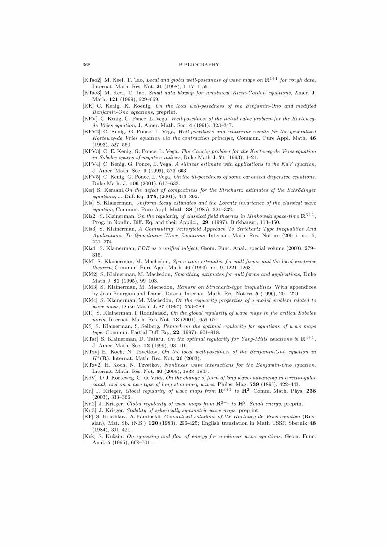
368 BIBLIOGRAPHY
[KTao2] M. Keel, T. Tao, Local and global well-posedness of wave maps on R1+1 for rough data,Internat. Math. Res. Not. 21 (1998), 1117–1156.
[KTao3] M. Keel, T. Tao, Small data blowup for semilinear Klein-Gordon equations, Amer. J.Math. 121 (1999), 629–669.
[KK] C. Kenig, K. Koenig, On the local well-posedness of the Benjamin-Ono and modifiedBenjamin-Ono equations, preprint.
[KPV] C. Kenig, G. Ponce, L. Vega, Well-posedness of the initial value problem for the Korteweg-de Vries equation, J. Amer. Math. Soc. 4 (1991), 323–347.
[KPV2] C. Kenig, G. Ponce, L. Vega, Well-posedness and scattering results for the generalizedKorteweg-de Vries equation via the contraction principle, Commun. Pure Appl. Math. 46
(1993), 527–560.[KPV3] C. E. Kenig, G. Ponce, L. Vega, The Cauchy problem for the Korteweg-de Vries equation
in Sobolev spaces of negative indices, Duke Math J. 71 (1993), 1–21.[KPV4] C. Kenig, G. Ponce, L. Vega, A bilinear estimate with applications to the KdV equation,
J. Amer. Math. Soc. 9 (1996), 573–603.[KPV5] C. Kenig, G. Ponce, L. Vega, On the ill-posedness of some canonical dispersive equations,
Duke Math. J. 106 (2001), 617–633.[Ker] S. Keraani,On the defect of compactness for the Strichartz estimates of the Schrodinger
equations, J. Diff. Eq. 175, (2001), 353–392.
[Kla] S. Klainerman, Uniform decay estimates and the Lorentz invariance of the classical waveequation, Commun. Pure Appl. Math. 38 (1985), 321–332.
[Kla2] S. Klainerman, On the regularity of classical field theories in Minkowski space-time R3+1,Prog. in Nonlin. Diff. Eq. and their Applic., 29, (1997), Birkhauser, 113–150.
[Kla3] S. Klainerman, A Commuting Vectorfield Approach To Strichartz Type Inequalities AndApplications To Quasilinear Wave Equations, Internat. Math. Res. Notices (2001), no. 5,221–274.
[Kla4] S. Klainerman, PDE as a unified subject, Geom. Func. Anal., special volume (2000), 279–315.
[KM] S. Klainerman, M. Machedon, Space-time estimates for null forms and the local existencetheorem, Commun. Pure Appl. Math. 46 (1993), no. 9, 1221–1268.
[KM2] S. Klainerman, M. Machedon, Smoothing estimates for null forms and applications, DukeMath J. 81 (1995), 99–103.
[KM3] S. Klainerman, M. Machedon, Remark on Strichartz-type inequalities. With appendicesby Jean Bourgain and Daniel Tataru. Internat. Math. Res. Notices 5 (1996), 201–220.
[KM4] S. Klainerman, M. Machedon, On the regularity properties of a model problem related towave maps, Duke Math. J. 87 (1997), 553–589.
[KR] S. Klainerman, I. Rodnianski, On the global regularity of wave maps in the critical Sobolevnorm, Internat. Math. Res. Not. 13 (2001), 656–677.
[KS] S. Klainerman, S. Selberg, Remark on the optimal regularity for equations of wave mapstype, Commun. Partial Diff. Eq., 22 (1997), 901–918.
[KTat] S. Klainerman, D. Tataru, On the optimal regularity for Yang-Mills equations in R4+1,J. Amer. Math. Soc. 12 (1999), 93–116.
[KTzv] H. Koch, N. Tzvetkov, On the local well-posedness of the Benjamin-Ono equation inHs(R), Internat. Math. Res. Not. 26 (2003).
[KTzv2] H. Koch, N. Tzvetkov, Nonlinear wave interactions for the Benjamin-Ono equation,Internat. Math. Res. Not. 30 (2005), 1833–1847.
[KdV] D.J. Korteweg, G. de Vries, On the change of form of long waves advancing in a rectangularcanal, and on a new type of long stationary waves, Philos. Mag. 539 (1895), 422–443.
[Kri] J. Krieger, Global regularity of wave maps from R3+1 to H2, Comm. Math. Phys. 238
(2003), 333–366.[Kri2] J. Krieger, Global regularity of wave maps from R2+1 to H2. Small energy, preprint.[Kri3] J. Krieger, Stability of spherically symmetric wave maps, preprint.[KF] S. Kruzhkov, A. Faminskii, Generalized solutions of the Korteweg-de Vries equation (Rus-
sian), Mat. Sb. (N.S.) 120 (1983), 296-425; English translation in Math USSR Sbornik 48
(1984), 391–421.[Kuk] S. Kuksin, On squeezing and flow of energy for nonlinear wave equations, Geom. Func.
Anal. 5 (1995), 668–701 .

BIBLIOGRAPHY 369
[Kuk2] S. Kuksin, Infinite-dimensional symplectic capacities and a squeezing theorem for Hamil-tonian PDE’s, Commun. Math. Phys. 167 (1995), 521–552.
[Kuk3] S. Kuksin, Analysis of Hamiltonian PDEs. Oxford Lecture Series in Mathematics and itsApplications, 19. Oxford University Press, Oxford, 2000.
[Kwo] M.K. Kwong, Uniqueness of positive solutions of ∆u−u+up = 0 in Rn, Arch. Rat. Mech.Anal. 105 (1989), 243–266.
[LShu] O.A. Ladyzhenskaya, V.I. Shubov, Unique solvability of the Cauchy problem for the equa-tions of the two dimensional chiral fields, taking values in complete Riemann manifolds, J.Soviet Math., 25 (1984), 855–864. (English Trans. of 1981 Article.)
[Leb] G. Lebeau, Nonlinear optics and supercritical wave equation, Bull. Soc. Roy. Sci. Liege, 70
(2002), 267-306. Hommage a Pascal Laubin.[Lem] L. Lemaire, Applications harmoniques de surfaces riemanniennes, J. Diff. Geom. 13 (1978).[LStr] J. Lin, W. Strauss, Decay and scattering of solutions of a nonlinear Schrodinger equation,
Journ. Funct. Anal. 30, (1978), 245–263.[Lin] H. Lindblad, A Sharp Counterexample to Local Existence of Low Regularity Solutions to
Nonlinear Wave Equations, Duke Math J., 72, (1993), 503–539.[LSog] H. Lindblad, C. D. Sogge, On Existence and Scattering with Minimal Regularity for Semi-
linear Wave Equations, Jour. Func. Anal., 130 (1995 ), 357–426.[LSog2] H. Lindblad, C. D. Sogge, Restriction theorems and semilinear Klein-Gordon equations
in (1+3) dimensions, Duke Math. J. 85 (1996), no. 1, 227–252.[MNNO] S. Machihara, M. Nakamura, K. Nakanishi, T. Ozawa, Endpoint Strichartz estimates
and global solutions for the nonlinear Dirac equation, J. Func. Anal. 219 (2005), 1–20.[MNO] S. Machihara, K. Nakanishi, T. Ozawa, Small global solutions and the nonrelativistic limit
for the nonlinear Dirac equation, Rev. Mat. Iberoamericana. 19 (2003), 179–194.[MNO2] S. Machihara, K. Nakanishi, T. Ozawa, Nonrelativistic limit in the energy space for
nonlinear Klein-Gordon equations, Math. Ann. 322 (2002), 603–621.[MSW] B. Marshall, W. Strauss, S. Wainger, Lp − Lq estimates for the Klein-Gordon equation,
J. Math. Pures Appl. (9) 59 (1980), no. 4, 417–440.[MN] N. Masmoudi, K. Nakanishi, From nonlinear Klein-Gordon equation to a system of coupled
nonlinear Schrdinger equations, Math. Ann. 324 (2002), no. 2, 359–389.[Mat] C. Matheus, Global well-posedness for a NLS-KdV system on T, preprint.[Mcl] K. McLeod, Uniqueness of positive radial solutions of ∆u + f(u) = 0 in Rn. II. Trans.
Amer. Math. Soc. 339 (1993), no. 2, 495–505.[Mer] F. Merle, Construction of solutions with exactly k blow-up points for the Schrodinger equa-
tion with critical non-linearity, Commun. Math. Phys. 149 (1992), 205–214.[Mer2] F. Merle, Determination of blow-up solutions with minimal mass for non-linear
Schrodinger equation with critical power, Duke Math. J. 69 (1993), 427–453.[Mer3] F. Merle, Asymptotics for L2 minimal blowup solutions of critical nonlinear Schrodinger
equation, Ann. Inst. Henri Poincare 13 (1996), 553–565.[MR] F. Merle, P. Raphael, Blowup dynamic and upper bound on the blowup rate for the critical
nonlinear Schrodinger equation, Ann. Math. 161 (2005), 157–222.[MR2] F. Merle, P. Raphael, Sharp upper bound on the blowup rate for the critical nonlinear
Schrodinger equation, GAFA 13 (2003), 591–642.[MR3] F. Merle, P. Raphael, On universality of blowup profile for L2 critical nonlinear
Schrodinger equation, Invent. Math. 156 (2004), 565–672.[Miu] R. Miura, Korteweg-de Vries equation and generalizations. I. A remarkable explicit non-
linear transformation, J. Mathematical. Phys. 9 (1968), 1202–1204.[Miu2] R. Miura, The Korteweg-de Vries Equation: A Survey of Results, SIAM Rev. 18(3) (1976),
412–459.[MST] L. Molinet, J.-C. Saut, N. Tzvetkov, Ill-posedness issues for the Benjamin-Ono and related
equations, SIAM J. Math. Anal. 33 (2001), 982–988.[Mon] S. J. Montgomery-Smith, Time Decay for the Bounded Mean Oscillation of Solutions of
the Schrodinger and Wave Equation, Duke Math J. 19 (1998), 393–408.[Mor] C. Morawetz, Time decay for the nonlinear Klein-Gordon equation, Proc. Roy. Soc. A 306
(1968), 291–296.[MS] S. Muller, M. Struwe, Global existence of wave maps in 1 + 2 dimensions with finite energy
data, Topological Methods in Analysis 7 (1996), 245–259.
370 BIBLIOGRAPHY
[MT] T. Muramatu, S. Taoka, The initial value problem for the 1-D semilinear Schrodingerequation in Besov spaces, J. Math. Soc. Japan 56 (2004), 853–888.
[NSU] A. Nahmod, A. Stefanov, K. Uhlenbeck, On the well-posedness of the wave map problemin high dimensions, Commun. Anal. Geom. 11 (2003), 49–83.
[Nak] K. Nakanishi, Scattering Theory for Nonlinear Klein-Gordon Equation with Sobolev CriticalPower, Internat. Math. Research Not. 31 (1999), 31-60.
[Nak2] K. Nakanishi, Energy scattering for non-linear Klein-Gordon and Schrodinger equationsin spatial dimensions 1 and 2, J. Func. Anal. 169 (1999), 201–225.
[Nak3] K. Nakanishi, Unique global existence and asymptotic behaviour of solutions for waveequations with non-coercive critical nonlinearity, Commun. Partial Differential Equations. 24
(1999), 185–221.[Nak3] K. Nakanishi, Local well-posedness and Illposedness in the critical Besov spaces for semi-
linear wave equations with quadratic forms, Funk. Ekvac. 42 (1999), 261-279.[Nak4] K. Nakanishi, Nonrelativistic limit of scattering theory for nonlinear Klein-Gordon equa-
tions, J. Differential Equations 180 (2002), no. 2, 453–470.[NTT] K. Nakanishi, H. Takaoka, Y. Tsutsumi, Counterexamples to bilinear estimates related with
the KdV equation and the nonlinear Schrodinger equation, Methods Appl. Anal. 8 (2001),569–578.
[Naw] H. Nawa, Asymptotic and limiting profiles of blowup solutions of the nonlinear Schrodinger
equation with critical power, Commun. Pure. Appl. Math. 52 (1999), 193–270.[Obe] D. Oberlin, Convolution estimates for some distributions with singularities on the light
cone, Duke Math. J. 59 (1989), 747–757.[Ono] H. Ono, Algebraic solitary waves in stratified fluids, J. Phys. Soc. Japan 39 (1975), 1082–
1091.[Oza] T. Ozawa, Long range scattering for nonlinear Schrodinger equations in one space dimen-
sion, Commun. Math. Phys. 139 (1991), 479–493.[Oza2] T. Ozawa, On nonlinear Schrodinger equations of derivative type, Indiana Univ. Math. J.
45 (1996), 137–163.[Pec] H. Pecher, Global solutions with infinite energy for the 1-dimensional Zakharov system,
preprint.[Pec2] H. Pecher, The Cauchy problem for a Schroedinger-Korteweg-de Vries system with rough
data, preprint.[Pec3] H. Pecher, Rough solutions of a Schroedinger-Benjamin-Ono system, preprint.[Poh] K. Pohlmeyer, Integrable Hamiltonian systems and interaction through quadratic con-
straints, Commun. Math. Phys., 46 (1976), 207–221.[Pon] G. Ponce, On the global well-posedness of the Benjamin-Ono equation, Diff. Int. Eq. 4
(1991), 527–542.[PS] G. Ponce, T. Sideris, Local regularity of nonlinear wave equations in three space dimensions,
Commun. Partial Diff. Eq. 18 (1983), 169–177.[Pri] P. Price, A montonicity formula for Yang-Mills fields, Manuscripta Math. 43 (1983), 131–
166.[Rau] J. Rauch, The u5 Klein-Gordon equation. II. Anomalous singularities for semilinear wave
equations in Nonlinear partial differential equations and their applications. College de FranceSeminar, Res. Notes in Math. 51, Pitman Publ.,(1981) 335–364.
[RR] J. Rauch, M. Reed, Nonlinear microlocal analysis of semilinear hyperbolic systems in onespace dimension, Duke Math. J., 49 (1982), 397–475.
[Ros] R. Rosales, I. Exact solution of some nonlinear evolution equations. II. The similaritysolution for the Korteweg-de Vries equation and the related Painleve transcendent, Ph. D.thesis, California Institute of Technology, 1977.
[RV] E. Ryckman, M. Visan, Global well-posedness and scattering for the defocusing energy-critical nonlinear Schrodinger equation in R1+4, preprint.
[SacU] J. Sacks, K. Uhlenbeck, The existence of minimal immersions of 2-spheres, Annals ofMath. (2) 113 (1981), 1–24.
[Sad] C. Sadosky, Interpolation of Operators and Singular Integrals, Marcel Dekker Inc., 1976.[Sau] J. C. Saut, Sur des generalisations de l’equation de Korteweg-de Vries, Universite de Paris-
Sud Departement de Mathematique, Orsay, (1978).[Sau2] J. C. Saut, Quelques generalisations de l’equation de Korteweg-de Vries. II, J. Differential
Equations 33 (1979), 320–335.
BIBLIOGRAPHY 371
[Sau3] J.C. Saut, Sur quelques generalizations de l’equation de Korteweg-de Vries, J. Math. PuresAppl. 58 (1979), 21-61.
[Schn] G. Schneider, Approximation of the Korteweg-de Vries equation by the non-linearSchrodinger equation, J. Differential Equations 147 (1998), 333–354.
[Scho] R. Schoen, Analytic aspects of the harmonic map problem, Math. Sci. Res. Inst. Publ. 2
(1984), Springer, Berlin, 321–358.[SchU] R. Schoen, K. Uhlenbeck, A regularity theory for harmonic maps, J. Diff. Geom. 17 (1982),
307–335.[SY] R. Schoen, S.T. Yau, Lectures on harmonic maps, Conference proceedings and Lecture notes
in Geometry and Topology, II. International Press.[Seg] I.E. Segal, Non-linear semi-groups, Ann. of Math. 78 (1963), 339–364.[Seg2] I.E. Segal, The global Cauchy problem for a relativistic scalar field with power interactions,
Bull. Soc. Math. France 91 (1963), 129–135.[Seg3] I. E. Segal, Space-time Decay for Solutions of Wave Equations, Adv. Math., 22 (1976),
304–311.[Sel] S. Selberg, Multilinear space-time estimates and applications to local existence theory for
non-linear wave equations, Princeton University Thesis.[Sha] J. Shatah, The Cauchy problem for harmonic maps on Minkowski space, in Proceed. Inter.
Congress of Math. 1994, Birkhauser, 1126–1132.
[Sha2] J. Shatah, Weak solutions and development of singularities of the SU(2) σ-model. Com-mun. Pure Appl. Math., 41 (1988), 459–469.
[SStra] J. Shatah, W. Strauss, Breathers as homoclinic geometric wave maps, Physics D 99
(1996), 113–133.[SStru] J. Shatah, M. Struwe, Regularity results for non-linear wave equations, Ann. of Math.
138 (1993) 503–518.[SStru2] J. Shatah, M. Struwe, Well Posedness in the energy space for semilinear wave equations
with critical growth, Inter. Math. Research Not., 7 (1994), 303–309.[SStru3] J. Shatah, M. Struwe, Geometric Wave Equations, Courant Lecture Notes in Mathemat-
ics 2 (1998).[SStru4] J. Shatah, M. Struwe, The Cauchy problem for wave maps, Internat. Math. Res. Not.
11 (2002) 555–571.[ST] J. Shatah, A. Tavildar-Zadeh, Regularity of harmonic maps from the Minkowski space into
rotationally symmetric manifolds., Commun. Pure Appl. Math. 45 (1992), 947–971.[ST2] J. Shatah, A. Tavildar-Zadeh, On the Cauchy problem for equivariant wave maps, Commun.
Pure Appl. Math., 47 (1994), 719–753.[Sid] T. Sideris, Global existence of harmonic maps in Minkowski space, Commun. Pure Appl.
Math., 42 (1989),1–13.[Sjo] P. Sjolin, Regularity of solutions to Schrodinger equations, Duke Math. J.,55 (1987), 699–
715.[SSog] H. Smith, C.D. Sogge, Global Strichartz estimates for nontrapping perturbations of the
Laplacian, Commun. PDE 25 (2000), 2171–2183.[Sog] C. D. Sogge, Lectures on Nonlinear Wave Equations, Monographs in Analysis II, Interna-
tional Press, 1995.[Sta] G. Staffilani, On the growth of high Sobolev norms of solutions for KdV and Schrodinger
equations, Duke Math J. 86 (1997), 109–142.[Stef] A. Stefanov, Strichartz estimates for the Schrodinger equation with radial data, Proc. Amer.
Math. Soc. 129 (2001), no. 5, 1395–1401.[Stei] E. M. Stein, Singular Integrals and Differentiability Properties of Functions, Princeton
University Press, 1970.[Stei2] E. M. Stein, Harmonic Analysis, Princeton University Press, 1993.[Stra] W. A. Strauss, Nonlinear wave equations, CBMS Regional Conference Series in Mathemat-
ics, no. 73, Amer. Math. Soc. Providence, RI, 1989.[Stri] R. S. Strichartz, Restriction of Fourier Transform to Quadratic Surfaces and Decay of
Solutions of Wave Equations, Duke Math. J., 44 (1977), 70 5–774.[Stri2] R. Strichartz, Asymptotic behavior of waves, J. Funct. Anal. 40 (1981), no. 3, 341–357.[Stru] M. Struwe, On the evolution of harmonic mappings of Riemannian surfaces, Comment.
Math. Helv. 60 (1985), 558–581.

372 BIBLIOGRAPHY
[Stru2] M. Struwe, Globally regular solutions to the u5 Klein-Gordon equation, Ann. Scuola Norm.Sup. Pisa Cl. Sci. 15 (1988), 495–513.
[Stru3] M. Struwe, Equivariant wave maps in two dimensions, Comm. Pure Appl. Math. 56
(2003), 815–823.[Stru4] M. Struwe, Radially symmetric wave maps from the (1+2)-dimensional Minkowski space
to a sphere, Math Z. 242 (2002), 407–414.[Stru5] M. Struwe, Radially symmetric wave maps from (1+2)-dimensional Minkowski space to
general targets, Calc. Var. 16 (2003), 431–437.[SSul] C. Sulem, P.-L. Sulem, The nonlinear Schrodinger equation: Self-focusing and wave col-
lapse, Springer-Verlag, New York, (1999), p. 25.[Tak] H. Takaoka, Well-posedness for the one-dimensional Schrodinger equation with the deriv-
ative nonlinearity, Adv. Diff. Eq. 4 (1999), 561–580.[Tao] T. Tao, Low regularity semi-linear wave equations, Commun. Partial Differential Equations,
24 (1999), no. 3-4, 599–629.[Tao2] T. Tao, Spherically averaged endpoint Strichartz estimates for the two-dimensional
Schrodinger equation, Commun. PDE 25 (2000), 1471–1485.[Tao3] T. Tao, Ill-posedness of one-dimensional wave maps at the critical regularity, Amer. J.
Math., 122 (2000), 451–463.[Tao4] T. Tao, Multilinear weighted convolution of L2 functions, and applications to non-linear
dispersive equations, Amer. J. Math. 123 (2001), 839–908.[Tao5] T. Tao, Global regularity of wave maps I. Small critical Sobolev norm in high dimension,
Internat. Math. Res. Not. 7 (2001), 299-328.[Tao6] T. Tao, Global well-posedness of wave maps II. Small energy in two dimensions, Commun.
Math. Phys. 224 (2001), 443–544.[Tao7] T. Tao, Global well-posedness of the Benjamin-Ono equation in H1(R), J. Hyperbolic Diff.
Eq. 1 (2004) 27–49.[Tao8] T. Tao, On the asymptotic behavior of large radial data for a focusing non-linear
Schrodinger equation, Dynamics of PDE 1 (2004), 1–48.[Tao9] T. Tao, Global well-posedness and scattering for the higher-dimensional energy-critical
non-linear Schrodinger equation for radial data, New York J. Math. 11 (2005), 57–80.[Tao10] T. Tao, Geometric renormalization of large energy wave maps, Journees EDP, Forges les
Eaux, 7-11 June 2004, XI 1–32..[Tao11] T. Tao, Recent progress on the Restriction conjecture, to appear, Park City Proceedings.[Tao12] T. Tao, Spacetime bounds for the energy-critical nonlinear wave equation in three spatial
dimensions, preprint.[TV] T. Tao, M. Visan, Stability of energy-critical nonlinear Schrodinger equations in high di-
mensions, Electron. J. Diff. Eq. 2005 (2005), No. 118, 1–28.[TVZ] T. Tao, M. Visan, X. Zhang, The nonlinear Schrodinger equation with power type nonlin-
earities, preprint.[Tat] D. Tataru, Local and global results for wave maps I, Commun. PDE 23 (1998), 1781–1793.[Tat2] D. Tataru, On global existence and scattering for the wave maps equation, Amer. J. Math.
123 (2001), 37–77.[Tat3] D. Tataru, On u = |∇u|2 in 5 + 1 dimensions, Math. Res. Letters 6 (1999), 469-485.[Tat4] D. Tataru, Rough solutions for the wave maps equation, Amer. J. Math. 127 (2005), 293–
377.[Tat5] D. Tataru, The wave maps equation, preprint.[Tay] M. Taylor, Partial Differential Equations I. Basic Theory, Applied Mathematical Sciences
115, Springer-Verlag, New York, Berlin, Heidelberg 1997.[Tay2] M. Taylor, Tools for PDE. Pseudodifferential operators, paradifferential operators, and
layer potentials. Mathematical Surveys and Monographs, 81. American Mathematical Society,Providence, RI, 2000.
[TU] C.L. Terng, K. Uhlenbeck, 1+1 wave maps into symmetric spaces, Comm. Anal. Geom. 12
(2004), 343–388.[Tom] M.M. Tom, Smoothing properties of some weak solutions of the Benjamin-Ono equation,
Diff. Int. Eq. 3 (1990) 683–694.[Tomas] P. Tomas, A restriction theorem for the Fourier transform, Bull. Amer. Math. Soc. 81
(1975), 477–478.
BIBLIOGRAPHY 373
[Tsu] Y. Tsutsumi, L2 solutions for nonlinear Schrodinger equations and nonlinear groups, Funk.Ekva. 30 (1987), 115–125.
[Tsu2] Y. Tsutsumi, The Cauchy problem for the Korteweg-de Vries equation with measures asinitial data, SIAM J. Math. Anal. 20 (1989), 582–588.
[Tzi] N. Tzirakis, The Cauchy problem for the semilinear quintic Schrodinger equation in onedimension 18 (2005).
[Tzv] N. Tzvetkov, Remark on the local ill-posedness for the KdV equation, C. R. Acad. Sci. Paris329 (1999), 1043–1047.
[Tzv2] N. Tzvetkov, Ill-posedness issues for nonlinear dispersive equations, lecture notes.[Tzv3] N. Tzvetkov, On the long time behavior of KdV type equations (after Martel-Merle),
Bourbaki seminar March 2004.[Uhl] K. Uhlenbeck, Connections with Lp bounds on curvature, Commun. Math. Phys 83, (1982)
31–42.[VV] A. Vargas, L. Vega, Global well-posedness for 1D nonlinear Schrodinger equation for data
with an infinite L2 norm, J. Math. Pures Appl. 80 (2001), 1029–1044.[Veg] L. Vega, Schrodinger equations: pointwise convergence to the initial data, Proc. Amer.
Math. Soc., 102 (1988), 874–878.[Vil] M. Vilela, Regularity of solutions to the free Schrodinger equation with radial initial data,
Illinois J. Math. 45 (2001), 361–370.
[Vil2] M. Vilela, Inhomogeneous Strichartz estimates for the Schrodinger equation, preprint.[Vis] M. Visan, The defocusing energy-critical nonlinear Schrodinger equation in dimensions four
and higher, Ph.D. thesis, in preparation.[Wei] M.I. Weinstein, Nonlinear Schrodinger equations and sharp interpolation estimates, Com-
mun. Math. Phys. 87 (1983), 567–576.[Wei2] M. Weinstein, Modulational stability of ground states of nonlinear Schrodinger equations,
SIAM J. Math. Anal. 16 (1985), 472–491.[Wei3] M. Weinstein, Lyapunov stability of ground states of nonlinear dispersive equations,
Comm. Pure Appl. Math. 39 (1986), 51-68.[Yaj] K. Yajima, Existence of solutions for Schrodinger evolution equations, Commun. Math.
Phys. 110 (1987), 415–426.[Zho] Y. Zhou, Global weak solutions for the 1 + 2 dimensional wave maps into homogeneous
spaces Ann. Inst. Henri Poincare (C) Analyse nonlineaire 16 (1999), 411–422.[Zho2] Y. Zhou, Uniqueness of weak solutions of 1 + 1 dimensional wave maps, Math. Z. 232
(1999), 707–719.[Zho3] Y. Zhou, Local existence with minimal regularity for nonlinear wave equations, Amer. J.
Math, 119 (1997), 671–703.