nonlinear control system design by quantifier elimination · we consider dynamical systems...

J. Symbolic Computation (1997) 24, 137–152

Nonlinear Control System Design by QuantifierElimination

MATS JIRSTRAND†

Department of Electrical Engineering,Linkoping University, S-581 83 Linkoping, Sweden

Many problems in control theory can be formulated as formulae in the first-order theoryof real closed fields. In this paper we investigate some of the expressive power of thistheory. We consider dynamical systems described by polynomial differential equationssubjected to constraints on control and system variables and show how to formulatequestions in the above framework which can be answered by quantifier elimination.The problems treated in this paper regard stationarity, stability, and following of apolynomially parametrized curve. The software package QEPCAD has been used tosolve a number of examples.

c© 1997 Academic Press Limited

1. Introduction

In this paper we discuss some applications of quantifier elimination for real closed fieldsto nonlinear control theory. Since the basic framework is real algebra and real algebraicgeometry we consider dynamical systems described by differential and non-differentialequations and inequalities in which all nonlinearities are of polynomial type. This rep-resents a rather large class of systems and it can be shown that systems where thenonlinearities are not originally polynomial can be rewritten in polynomial form if thenonlinearities themselves are solutions to algebraic differential equations. For more detailson this, see Rubel and Singer (1985) and Lindskog (1996).

Given a state space description of a dynamical system (i.e. the system is described bya number of first-order differential equations, so-called state equations) and constraintson the states as well as on the control signals we consider three classes of problems whichcan be solved by quantifier elimination.

(i) Which states correspond to equilibrium points of the system for some admissiblecontrol signal and which stability properties do these equilibrium points have?

(ii) Which output levels correspond to stable equilibrium points and is it possible tomove between different stable equilibrium points for some control signal?

(iii) Given a parametrized curve in the state space of the system. Is it possible tofollow the curve by using available control signals? More general, given a set ofparametrized curves. Which states can be reached by following one of these curves?

† E-mail: [email protected], URL: http://www.control.isy.liu.se

0747–7171/97/020137 + 16 $25.00/0 sy970119 c© 1997 Academic Press Limited

138 M. Jirstrand

Stationary (equilibrium, critical) points play an important role in both analysis anddesign of dynamical systems and for synthesis of control laws. These points are the onlypossible operating points of the system and often a control law is designed such that thestate of the system will return to such a point after moderate disturbances. The set ofequilibrium points of a dynamical system is parametrized by the available control signalsand the first problem addresses the construction of this set for polynomial systems.

The second problem is important in a wide variety of control applications since it givesinformation about the range of the output in which the system can be controlled in a“safe” way.

The last problem is a natural question in many control situations where the objectiveis to steer the dynamical system from one point to another along a certain path. Observethat the prescribed path belongs to the state space, which implies that the whole systemdynamics is specified. Hence this is an extension of the motion planning problem also tak-ing into account the system dynamics. This problem is also generalized to a constrainedform of computable reachability.

Classical approaches to the aforementioned problems are numerical solutions of systemsof nonlinear equations and simulations studies, see Stevens and Lewis (1992), Ljung andGlad (1994) and Dennis and Schnabel (1983). A drawback of these techniques are thedifficulties to verify that all solutions of the problem have been found. It is also hardto study how solutions depend on different parameters in the equations since a newcomputation has to be done for each new value of a parameter.

For control-system design it is valuable to have symbolic expressions of performanceconstraints in terms of design parameters since it facilitates both optimal and robustchoices of these parameters. The absence of such expressions is usually replaced by ex-tensive simulation studies to get a feasible design.

One of the first attempts to apply quantifier elimination techniques to problems incontrol theory was made by Anderson et al. (1975). However, the algorithmic techniquesat that time were very complex and no computer software were available. Recently,a few papers treating control-related problems have appeared (Glad, 1995; Abdallahet al., 1996; Syrmos et al., 1996; Blondel and Tsitsiklis, 1995) and since the seventiesthere has been considerable progress in the development of more effective quantifierelimination algorithms starting with Collins (1975). For an extensive bibliography seeArnon (1988) and more recent work by Hong (1992a, 1992b).

In the control community there is a growing interest to use inequalities in modelingof dynamical systems, see Willems (1995). Also in optimal control it is very common tohave inequality constraints on both the control and system variables, see Bryson and Ho(1969). However, the existence of algorithms for symbolic computation with systems ofpolynomial equations and inequalities have still not yet been fully recognized.

We suppose that the reader is familiar with some basic concepts from (real) algebra andreal algebraic geometry, such as ideals, algebraic sets, semi-algebraic sets and quantifierelimination. Some references are Cox et al. (1992), Bochnak et al. (1987), Benedetti andRisler (1990), Davenport et al. (1988) and Mishra (1991).

To denote algebraic and semi-algebraic sets we use calligraphic letters such as S andthe defining formula of the set is denoted S(x), i.e. S = {x ∈ Rn | S(x)}.

To perform quantifier elimination in the non-trivial examples of this paper we haveused the program QEPCAD (v.13-aug94), developed by Hoon Hong and co-workers atRISC in Austria, see Collins and Hong (1991).

The paper is organized as follows. In Section 2 stationary points and their stability

Nonlinear Control System Design by Quantifier Elimination 139

properties are discussed. Section 3 discusses the question of the possiblity of steering asystem between different stable stationary points. The question of whether the states ofa system can follow a parametrized curve is discussed in Section 4 and Section 5 containsconclusions and some extensions.

2. Stationarizable Sets

It will be assumed that the dynamical system is described by a nonlinear differentialequation written in state-space form

x = f(x, u)y = h(x)

(2.1)

where x is a n-vector, u a m-vector, y a p-vector and each component of f and h is areal polynomial, fi ∈ R[x, u], hj ∈ R[x]. The x, u and y vectors will be referred to as thestate, control, and output of the system respectively.

Suppose also that the system variables have to obey some additional constraints

x ∈ X and u ∈ U , (2.2)

where X and U are semi-algebraic sets which define the constraints on the state andcontrol variables. We call x ∈ X the admissible states and u ∈ U the admissible controls.

A variety of constraints can be represented in the semi-algebraic framework, e.g. am-plitude and direction constraints.

Example 2.1. Let F be a two-dimensional thrust vector which can be pointed in anydirection φ and whose magnitude |F | can be varied between 0 and Fmax . Let

u1 = cos(φ), u2 = sin(φ), and u3 = |F |.Then the semi-algebraic set describing these constraints becomes

U = {u ∈ R3 | u21 + u2

2 = 1 ∧ 0 ≤ u3 ≤ Fmax}.Similarly, constraints on the states may originate from specifications on the system out-puts, e.g. |h(x)| ≤ ε.

The main question in this section concerns equilibrium or stationary points of a dy-namical system, i.e. solutions of (2.1) that correspond to constant values of the admissiblestates and controls. In other words, we are interested in those admissible states for whichthe system can be kept at rest by using an admissible control. The conditions for a point,x0 to be stationary is easily seen to be f(x0, u0) = 0 where x0 ∈ X and u0 ∈ U . For theclass of dynamical systems considered here, this set of stationarizable states turns out tobe a semi-algebraic set.

Definition 2.1. The stationarizable states of system (2.1) subjected to the constraints (2.2)is the set of states satisfying the formula

S(x) 4= ∃u[f(x, u) = 0 ∧ X (x) ∧ U(u)

]. (2.3)

The computation of a “closed form” of the set of stationarizable states, i.e. an ex-pression not including u, is a quantifier elimination problem and hence this set is semi-algebraic.

140 M. Jirstrand

-1

-0.5

0.5

1

x2

0.2 0.4

x1

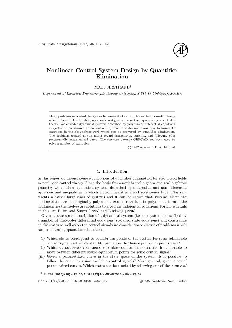
Figure 1. The stationarizable set (bold curve) of system (2.4) subjected to the control

constraints |u| ≤ 12

.

Example 2.2. Consider the following system

x1 = −x1 + x2u

x2 = −x2 + (1 + x21)u+ u3 (2.4)

subjected to the constraints

− 12 ≤ u ≤ 1

2 .

According to Definition 2.1 the stationarizable set is described by the formula

∃u[−x1 + x2u = 0 ∧ −x2 + (1 + x2

1)u+ u3 = 0 ∧ −12 ≤ u ≤ 1

2

],

which after quantifier elimination becomes[x4

2 − x31x

22 − x1x

22 − x3

1 = 0 ∧ [x2 + 2x1 ≤ 0 ∨ x2 − 2x1 ≥ 0]].

In this case the stationarizable set is easy to visualize, see Figure 1.

As an example of a specific application of the stationarizability result we consider thecontrol of an aircraft.

Example 2.3. In advanced aircraft applications the orientation of the aircraft withrespect to the airflow can be controlled. The orientation is usually described by the angleof attack α and sideslip angle β of the aircraft, see Figure 2.

An interesting question is for which α and β the orientation of the aircraft can be keptconstant by admissible control-surface configurations? It can be shown using the equationsof motion of an aircraft, see e.g. Stevens and Lewis (1992), that α and β are constant ifthe aerodynamic moments acting on the aircraft are zero. These moments are nonlinearfunctions of α, β, and the control-surface deflections, and they are usually given in tabularform together with some interpolation method. In Stevens and Lewis (1992) these tablesare listed for an F-16 aircraft and the following are scaled polynomial approximations of


x-axis(body)

x-axis(stability)

α

β

Relative wind

x-axis(wind)

z-axis(body)

y-axis(body)

Figure 2. The orientation of an aircraft with respect to the airflow.

the corresponding functions

CL(x1, x2, u1, u3) =− 38x2 − 170x1x2 + 148x21x2 + 4x3

2

+ u1(−52− 2x1 + 114x21 − 79x3

1 + 7x22 + 14x1x

22)

+ u3(14− 10x1 + 37x21 − 48x3

1 + 8x41 − 13x2

2 − 13x1x22

+ 20x21x

22 + 11x4

2)

CM (x1, u2) =− 12− 125u2 + u22 + 6u3

2 + 95x1 − 21u2x1 + 17u22x1

− 202x21 + 81u2x

21 + 139x3

1

CN (x1, x2, u1, u3) =139x2 − 112x1x2 − 388x21x2 + 215x3

1x2 − 38x32 + 185x1x

32

+ u1(−11 + 35x1 − 22x21 + 5x2

2 + 10x31 − 17x1x

22)

+ u3(−44 + 3x1 − 63x21 + 34x2

2 + 142x31 + 63x1x

22 − 54x4

1

− 69x21x

22 − 26x4

2)

where x1 is the normalized angle of attack, x2 is the sideslip angle, and u1, u2 and u3

are the aileron, elevator, and rudder deflections respectively.The question of constant orientation may now be posed as

∃u1 ∃u2 ∃u3

[CL = 0 ∧ CM = 0 ∧ CN = 0 ∧ u2

i ≤ 1, i = 1, 2, 3],

where the answer, a formula in x1 and x2, defines the semi-algebraic set describing thepossible stationarizable angles of attack and sideslip angles.

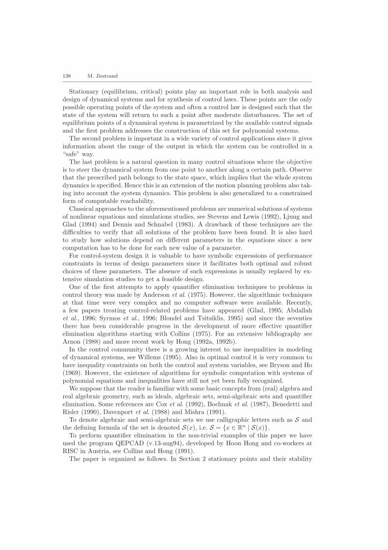
Elimination of u1 and u3 is easy since they appear linearly in the expressions. Toeliminate u2 we utilize QEPCAD and the complete solution is visualized in Figure 3.The limits on x1 obtained when u2 is eliminated from CM = 0 are outside the valid rangeof the polynomial approximations and is not shown in the figure. Observe that Figure 3shows that there is no problem to keep the aircraft at a constant angle of attack when thesideslip angle is small.

A prediction of possible, stationary orientations of an aircraft is usually carried out bynon-symbolic techniques, typically simulation studies and test flights. The advantage of

142 M. Jirstrand

0 0.2 0.4 0.6 0.8 1

x1

-1

-0.5

0

0.5

1

x2

Figure 3. Region (white) in the x1x2-plane corresponding to stationary orientations of the aircraft inExample 2.3.

the approach in this example is that we can get closed-form expressions for stationaryorientations in terms of design parameters of the aircraft. Furthermore, these expressionscan then be utilized to choose optimal values of these parameters.

Further applications of quantifier elimination to equilibrium calculations for nonlinearaircraft dynamics are presented in Jirstrand and Glad (1996b).

In stability theory for nonlinear dynamical systems one is often interested in the char-acter of the solution in a neighborhood of a stationary point. If all solutions startingin some neighborhood of a stationary point, x0, stays within this neighborhood for allfuture times the stationary point is called stable. If in addition the solutions convergetowards x0, the stationary point is called (locally) asymptotically stable. For an extensivetreatment of stability of dynamical systems see Hahn (1967).

The following theorem gives a sufficient condition for asymptotic stability of a station-ary point.

Theorem 2.1. Let x0 be a stationary point of system (2.1) corresponding to u = u0.Then x0 is asymptotically stable if all eigenvalues of fx(x0, u0) have a strictly negativereal part.

Proof. See Hahn (1967). 2

This result follows from the Taylor expansion

f(x, u) = f(x0, u0) + fx(x0, u0)(x− x0) + · · ·noting that f(x0, u0) = 0 since x0 is a stationary point and that the linear part of theexpansion is a good approximation of the original system near x0.

Since the eigenvalues of a matrix are the zeros of its characteristic polynomial we areinterested in determining if all the zeros of this polynomial have strictly negative realparts. The question can be answered in a number of different ways, by examining the


coefficients of the characteristic polynomial, e.g. by the criteria of Hurwitz, Routh orLienard-Chipart, see e.g. Parks and Hahn (1993) or Gantmacher (1971).

These criteria states that the zeros of a polynomial, p, have a strictly negative real partif and only if a number of strict polynomial inequalities, constructed from the coefficientsof p, is satisfied. Here we present one formulation of the Lienard-Chipart criterion.

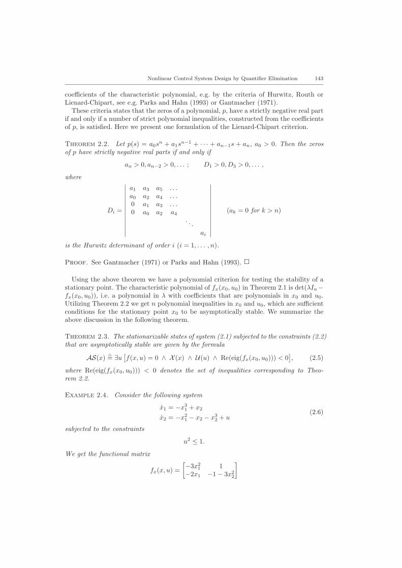
Theorem 2.2. Let p(s) = a0sn + a1s

n−1 + · · · + an−1s + an, a0 > 0. Then the zerosof p have strictly negative real parts if and only if

an > 0, an−2 > 0, . . . ; D1 > 0, D3 > 0, . . . ,

where

Di =

∣∣∣∣∣∣∣∣∣∣∣∣∣

a1 a3 a5 . . .a0 a2 a4 . . .0 a1 a3 . . .0 a0 a2 a4

. . .ai

∣∣∣∣∣∣∣∣∣∣∣∣∣(ak = 0 for k > n)

is the Hurwitz determinant of order i (i = 1, . . . , n).

Proof. See Gantmacher (1971) or Parks and Hahn (1993). 2

Using the above theorem we have a polynomial criterion for testing the stability of astationary point. The characteristic polynomial of fx(x0, u0) in Theorem 2.1 is det(λIn−fx(x0, u0)), i.e. a polynomial in λ with coefficients that are polynomials in x0 and u0.Utilizing Theorem 2.2 we get n polynomial inequalities in x0 and u0, which are sufficientconditions for the stationary point x0 to be asymptotically stable. We summarize theabove discussion in the following theorem.

Theorem 2.3. The stationarizable states of system (2.1) subjected to the constraints (2.2)that are asymptotically stable are given by the formula

AS(x) 4= ∃u[f(x, u) = 0 ∧ X (x) ∧ U(u) ∧ Re(eig(fx(x0, u0))) < 0

], (2.5)

where Re(eig(fx(x0, u0))) < 0 denotes the set of inequalities corresponding to Theo-rem 2.2.


x1 = −x31 + x2

x2 = −x21 − x2 − x3

2 + u(2.6)


u2 ≤ 1.

We get the functional matrix

fx(x, u) =[−3x2

1 1−2x1 −1− 3x2

2

]

144 M. Jirstrand

-1

-2

-1

0

1

2x2

-2 0 1 2

x1

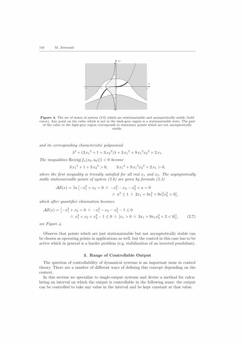
Figure 4. The set of states of system (2.6) which are stationarizable and asymptotically stable (boldcurve). Any point on the cubic which is not in the dark-grey region is a stationarizable state. The part

of the cubic in the light-grey region corresponds to stationary points which are not asymptoticallystable.

and its corresponding characteristic polynomial

λ2 + (3x12 + 1 + 3x2

2)λ+ 3x12 + 9x1

2x22 + 2x1.

The inequalities Re(eig(fx(x0, u0))) < 0 become

3x12 + 1 + 3x2

2 > 0, 3x12 + 9x1

2x22 + 2x1 > 0,

where the first inequality is trivially satisfied for all real x1 and x2. The asymptoticallystable stationarizable points of system (2.6) are given by formula (2.5)

AS(x) = ∃u[−x3

1 + x2 = 0 ∧ −x21 − x2 − x3

2 + u = 0

∧ u2 ≤ 1 ∧ 2x1 + 3x21 + 9x2

1x22 > 0

],

which after quantifier elimination becomes

AS(x) =[−x3

1 + x2 = 0 ∧ −x21 − x2 − x3

2 − 1 ≤ 0

∧ x21 + x2 + x3

2 − 1 ≤ 0 ∧ [x1 > 0 ∨ 3x1 + 9x1x22 + 2 < 0]

], (2.7)

see Figure 4.

Observe that points which are just stationarizable but not asymptotically stable canbe chosen as operating points in applications as well, but the control in this case has to beactive which in general is a harder problem (e.g. stabilization of an inverted pendulum).

3. Range of Controllable Output

The question of controllability of dynamical systems is an important issue in controltheory. There are a number of different ways of defining this concept depending on thecontext.

In this section we specialize to single-output systems and devise a method for calcu-lating an interval on which the output is controllable in the following sense: the outputcan be controlled to take any value in the interval and be kept constant at that value.


The outputs corresponding to the asymptotically stable, stationarizable states areeasily calculated as the projection of these states onto the output, i.e.

∃x[y = h(x) ∧ AS(x)

].

From this information we only know that there is an admissible control, u, such thatthe output, y, may be kept at a constant level despite small disturbances. What happenswith y when we change u by a small amount? Is it possible to change u such that yincreases or decreases to a new constant level? An examination of the output map,y = h(x) gives no information since u does not appear explicitly in this expression.However, since we assume that u effects y in some way u has to appear explicitly in someof the time derivatives of y. The lowest order of the time derivative of y where u appearsexplicitly is usually called the relative degree of the dynamical system, see Isidori (1995).

Let y(r) denote this derivative. For a stationary state the output y is constant andhence all derivatives are zero. If it is possible to change u such that y(r) > 0 all lowerderivatives becomes positive after an infinitesimal amount of time and y increases. Thesubset of the asymptotically stable, stationarizable states for which this is possible isdescribed by the formula

AS+(x) 4= ∃u[AS(x) ∧ y(r) > 0 ∧ U(u)

]. (3.1)

The formula for states in AS(x) corresponding to decreasing y is obtained in the sameway and becomes

AS−(x) 4= ∃u[AS(x) ∧ y(r) < 0 ∧ U(u)

]. (3.2)

Combining these formulae we get the states for which both an increase and a decreaseof the output is possible

CS(x) 4= AS+(x) ∧ AS−(x). (3.3)

The corresponding output range is the projection of this set onto y

CO(y) 4= ∃x[y = h(x) ∧ CS(x)

], (3.4)

which we will call the controllable output range of the dynamical system.

Example 3.1. Consider the system in Example 2.4 and let y = x1, where the asymptot-ically stable, stationarizable set is given by (2.7). Since

y = x1 = −x31 + x2, y = −3x2

1x1 + x2 = −3x21(−x3

1 + x2)− x21 − x2 − x3

2 + u,

the relative degree of this system is 2 and the asymptotically stable, stationarizable statesfor which y can be increased or decreased becomes

AS+(x) = ∃u[AS(x) ∧ −x2

1 + 3x51 − 3x2

1x2 − x2 − x32 + u > 0 ∧ u2 ≤ 1

],

AS−(x) = ∃u[AS(x) ∧ −x2

1 + 3x51 − 3x2

1x2 − x2 − x32 + u < 0 ∧ u2 ≤ 1

],

CS(x) = AS+(x) ∧ AS−(x).

In this case it can be shown that the semi-algebraic set described by CS(x) is the same asAS(x) except for some points on the border of AS(x). The controllable output range ofthis system is

CO(y) = ∃x[y = h(x) ∧ CS(x)

]=[[y + 1 > 0 ∧ 9y7 + 3y + 2 < 0] ∨ [y > 0 ∧ y9 + y3 + y2 − 1 < 0]

]=[[−1 < y < −0.591 . . . ] ∨ [0 < y < 0.735 . . . ]

].

146 M. Jirstrand

−1 −0.5 0 0.5 1

−1

−0.5

0

0.5

1

u= −0.5

u= −0.05

u = −0.05

u=0.75

Figure 5. The phase portrait corresponding to a number of different controls.

Compare the controllable output range with the projection on the x1-axis of the states inExample 2.4 which are both stationarizable and asymptotically stable.

The character of solutions to system (2.6) with initial values near the points in CS isshown in Figure 5 where the phase portrait for a number of different admissible controlsis shown.

Observe that an output interval in CO might be composed by subintervals, whichcorresponds to projections of several disjoint parts of the state space. If this is the caseit might happen that we cannot steer the output from a point on one subinterval to apoint on another subinterval.

4. Following a Parametrized Curve

Consider a parametrized curve C in Rn

C : x = g(t), t ∈ [α, β], g : R→ Rn,

whose orientation is defined by increasing t and all components of g are polynomials in t.Given the system (2.1) subjected to the semi-algebraic state and control constraints (2.2)is it then possible to steer the system from the initial state x0 = g(α) to the final statex1 = g(β) along the curve?

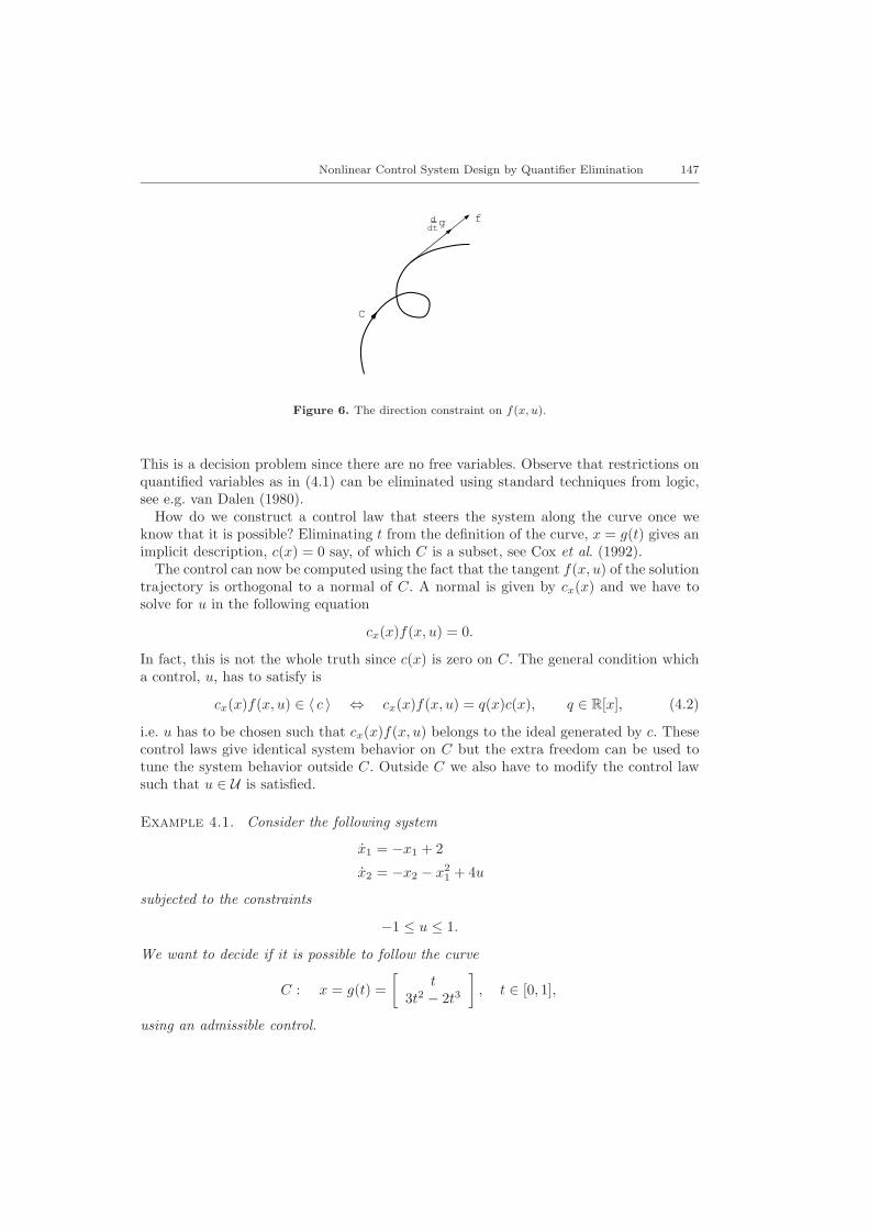
To steer the system along the curve there has to be an admissible control u at eachpoint on the curve such that the solution trajectory tangent vector, f(x, u) points in thesame direction as a forward-pointing tangent vector of the curve, i.e.

f(g(t), u) = λd

dtg(t), λ > 0, t ∈ [α, β],

see Figure 6.The above question can be formulated as a quantifier elimination problem as follows:(

∀t ∈ [α, β])(∃u ∈ U

)(∃λ > 0

)[f(g(t), u) = λ

d

dtg(t)

]. (4.1)


f

C

gddt−

Figure 6. The direction constraint on f(x, u).

This is a decision problem since there are no free variables. Observe that restrictions onquantified variables as in (4.1) can be eliminated using standard techniques from logic,see e.g. van Dalen (1980).

How do we construct a control law that steers the system along the curve once weknow that it is possible? Eliminating t from the definition of the curve, x = g(t) gives animplicit description, c(x) = 0 say, of which C is a subset, see Cox et al. (1992).

The control can now be computed using the fact that the tangent f(x, u) of the solutiontrajectory is orthogonal to a normal of C. A normal is given by cx(x) and we have tosolve for u in the following equation

cx(x)f(x, u) = 0.

In fact, this is not the whole truth since c(x) is zero on C. The general condition whicha control, u, has to satisfy is

cx(x)f(x, u) ∈ 〈 c 〉 ⇔ cx(x)f(x, u) = q(x)c(x), q ∈ R[x], (4.2)

i.e. u has to be chosen such that cx(x)f(x, u) belongs to the ideal generated by c. Thesecontrol laws give identical system behavior on C but the extra freedom can be used totune the system behavior outside C. Outside C we also have to modify the control lawsuch that u ∈ U is satisfied.


x1 = −x1 + 2

x2 = −x2 − x21 + 4u


−1 ≤ u ≤ 1.

We want to decide if it is possible to follow the curve

C : x = g(t) =[

t3t2 − 2t3

], t ∈ [0, 1],

using an admissible control.

148 M. Jirstrand

The quantifier formulation (4.1) of the problem becomes(∀t ∈ [0, 1]

)(∃u ∈ [−1, 1]

)(∃λ > 0

)[−t+ 2 = λ ∧ −(3t2 − 2t3)− t2 + 4u = λ(6t− 6t2)

],

which can be shown to be true!We now compute the control laws that steer the system along C. An implicit description

of C is x2 − 3x21 + 2x3

1 = 0 and the orthogonality condition (4.2) gives

(−6x1 + 6x21)(−x1 + 2)− x2 − x2

1 + 4u ∈ 〈x2 − 3x21 + 2x3

1〉.

In general one has to check that the chosen control law steers the system in the rightdirection along C. In this example we know that there exists a control law that steers thesystem in the right direction on C but there is also only one way of choosing u modulo 〈c〉on C. Hence any of the above u can be chosen, e.g.

u =32x3

1 −174x2

1 + 3x1 +14x2,

which is a state feedback control law that steers the system along C in the right direction.

4.1. constrained reachability

The important concept of reachability, i.e. questions about which states can be reachedfrom a given set of initial states by a system, is not in general solvable by algebraicmethods. The reason is that generically the solution trajectory of a system of differentialequations such as (2.1) is not an algebraic set or even a subset thereof. However, a morerestricted form of reachability can be investigated using semi-algebraic tools.

Let I be a semi-algebraic set defining possible initial states of system (2.1) and C afamily of parametrized curves

C = {C : x = g(t;x0, x1, θ), t ∈ [α, β] | I(g(α))},

where each component of g is a polynomial in t, x0, x1, θ and g(α) = x0, g(β) = x1.Here θ denotes some additional parameters to get more flexibility.

Definition 4.1. We say that a curve, C ∈ C is admissible if all points on C belongto the admissible states X and there is an admissible control u such that the solutiontrajectory of (2.1) follows C.

Definition 4.2. The set R(I) ⊆ X which can be reached by using an admissible con-trol u such that the solution trajectory of (2.1) follows one of the curves in C is calledthe C-reachable set w.r.t. I.

Using a family, C of parametrized curves which are very flexible (e.g. Bezier curves, seeCox et al. (1992)) the C-reachable set w.r.t. some set of possible initial states should bea good approximation to the ordinary reachable set.

The computation of the setR(I) can be carried out by quantifier elimination as follows.The condition on the initial points of curves in C and the first condition in Definition 4.1are easily semi-algebraically characterized as I(x0) ∧ X (g(t;x0, x1, θ) and the second


condition in Definition 4.1 is the one just treated above. We get the following semi-algebraic characterization(

∃θ ∈ Θ)(∃x0 ∈ I

)(∀t ∈ [α, β]

)(∃u ∈ U

)(∃λ > 0

)[f(g(t), u) = λ

d

dtg(t) ∧ X (g(t))

]. (4.3)

After quantifier elimination we get a real polynomial system in x1 defining the C-reachableset w.r.t. I.


x1 = x1 + u

x2 = x22

(4.4)

subjected to the control constraints

−1 ≤ u ≤ 1.

Which states are reachable along straight lines from the point (x1, x2) = (0, 1)?The set of initial states is

I = {x0 ∈ R2 | x01 = 0 ∧ x0

2 = 1}and a parametrization of straight lines from (x0

1, x02) to (x1

1, x12) is

C : x = g(t) = t

[x1

1 − x01

x12 − x0

2

]+

[x0

1

x02

], t ∈ [0, 1].

Formula (4.3) becomes(∀t ∈ [0, 1]

)(∃u ∈ [−1, 1]

)(∃λ > 0

)[tx1

1 + u = λx11 ∧ (t(x1

2 − 1) + 1)2 = λ(x12 − 1)

](4.5)

and eliminating quantifiers we get[−x1

1(x12)2 + x1

1x12 − x1

2 − x11 + 1 ≤ 0 ∧

x11(x1

2)2 − x11x

12 − x1

2 + x11 + 1 ≤ 0

],

(4.6)

see Figure 7.A control law that steers the system along a straight line can be computed as in Exam-

ple 4.1 observing that C with slope k is a part of the zero set of c(x) = x2− 1− kx1. Theorthogonality condition (4.2) with the choice q(x) = 0 gives

−k(x1 + u) + x22 = 0 ⇒ u =

1kx2

2 − x1, k 6= 0.

The cases k = 0 and k = ∞ cause no problems since the line x2 = 1 does not belong toR(I) and for k =∞ the control law simply becomes u = −x1. Furthermore, this controllaw steers the system in the right direction.

Once we know the set of reachable states from a point along straight lines an obviousgeneralization is to let this set be possible initial states of a new calculation of reachability.The resulting set would be an even better approximation to the real reachable set of

150 M. Jirstrand

x1

2

1

0

3

4

5

x2

-1 0 1

u=-1 u=+1

Figure 7. The semi-algebraic set defined by (4.6) (grey shaded region) that can be reached from (0, 1)by following a straight line using an admissible control. The set that is reachable from (0, 1) by any

admissible control corresponds to the region above the solutions labelled u = +1 and u = −1.

states. Unfortunately, this calculation was to a complex to be carried out by our versionof the QEPCAD program.

5. Conclusions and Extensions

In this paper we have formulated a number of problems in nonlinear control theoryas formulae in the first-order theory of real closed fields. First, stationary points of adynamical system subject to control and state constraints was treated. Second, the cal-culation of output intervals on which one has “complete” control over the output wasinvestigated, and finally the ability of a dynamic system to follow an algebraic curve wasstudied. In connection with the last problem we also investigated a constrained form ofcomputable reachability.

In all problems it is possible to take into account constraints on both the control andstate variables. This makes this framework very attractive since these constraints arevery common in practice but hard to take into consideration using classical methods.The problems in this paper can all be treated successfully by quantifier eliminationmethods and the main advantage of these methods is the symbolic form of the result.This is especially important when the result contains design parameters of the systemthat have to be determined. The symbolic form often facilitates an optimal choice ofthese parameters.

In principle nothing prevents us from working with systems given in implicit form,f(x, x, u) = 0 or more general mixed-state and control constraints, U(x, u) but we havechosen a simpler setting to demonstrate the ideas.

Many problems in control theory seem to fit into the framework described in thispaper. Some further examples of areas in control theory where applications of quantifierelimination methods could be investigated are as follows.


(i) Feedback design of linear dynamical systems, see Maciejowski (1989). Stability andperformance constraints are often given as semi-algebraic constraints on the so-called Nyquist curve.

(ii) Stability analysis using the circle and Popov criterion, see Vidyasagar (1993).(iii) Computation of robustness regions of nonlinear state feedback, see Glad (1987).(iv) Stability analysis of nonlinear systems using Lyapunov methods, see Hahn (1967).(v) Control law verification of linear dynamical systems, i.e. to determine if a given

control law results in the desired performance.

The interested reader is referred to Jirstrand (1996a) for investigations of some of theabove problems.

The main drawback of the quantifier elimination algorithms are that they have a ratherbad time-complexity w.r.t. the number of variables which at present limits its usefulnessfor large-scale control applications.

Acknowledgements

This work was supported by the Swedish Research Council for Engineering Sciences(TFR), which is gratefully acknowledged. The author is also grateful to Dr Hoon Hongat RISC, Austria for providing him with a copy of the QEPCAD program.

References——Abdallah, C.T., Dorato, P., Yang, W., Liska, R., Steinberg, S. (1996). Applications of quantifier elimination

theory to control system design. In Proceedings of the 4th IEEE Mediterranean Symposium onControl and Automation, 10–14 June, 1996, Crete, Greece, pp. 340–345.

——Anderson, B., Bose, N., Jury, E. (1975). Output feedback stabilization and related problems—solutionvia decision methods. IEEE Trans. Automat. Control, AC-20(1), 53–65.

——Arnon, D. (1988). A bibliography of quantifier elimination for real closed fields. J. Symbolic Comput.,5(1, 2), 267–274.

——Benedetti, R., Risler, J. (1990). Real Algebraic and Semi-Algebraic Sets. Paris, Hermann.——Blondel, V.D., Tsitsiklis, J.N. (1995). NP-hardness of some linear control design problems. In Proceedings

of the ECC’95, European Control Conference, Isidori, A., ed., volume 3, pp. 2066–2071, Roma,Italy, Springer-Verlag.

——Bochnak, J., Coste, M., Roy, M.-F. (1987). Geometrie algebrique reelle. Springer.——Bryson, A.E., Ho, Y.C. (1969). Applied Optimal Control. Ginn and Company.——Collins, G. (1975). Quantifier elimination for real closed fields by cylindrical algebraic decomposition. In

Second GI Conference on Automata Theory and Formal Languages, Kaiserslauten. Lecture Notesin Comput. Sci.33, pp. 134–183. Springer.

——Collins, G., Hong, H. (1991). Partial cylindrical algebraic decomposition in quantifier elimination. J.Symbolic Comput., 12(3), 299–328.

——Cox, D., Little, J., O’Shea, D. (1992). Ideals, Varieties, and Algorithms: An Introduction to ComputationalAlgebraic Geometry and Commutative Algebra. Springer.

——Davenport, J., Siret, Y., Tournier, E. (1988). Computer Algebra. Systems and Algorithms for AlgebraicComputation. Academic Press.

——Dennis, J.E., Schnabel, R.B. (1983). Numerical Methods for Unconstrained Optimization and NonlinearEquations. Prentice Hall.

——Gantmacher, F. (1971). Matrix Theory, volume II. Chelsea.——Glad, S.T. (1987). Robustness of nonlinear state feedback—a survey. Automatica, 23(4), 425–435.——Glad, S.T. (1995). An algebraic approach to bang-bang control. In Proceedings of the ECC’95, European

Control Conference, Isidori, A., ed., volume 4, pp. 2892–2895, Rome, Italy, Springer-Verlag.——Hahn, W. (1967). Stability of Motion. Springer.——Hong, H. (1992a). Improvements in CAD-based quantifier elimination. PhD Thesis. The Ohio State

University.——Hong, H. (1992b). Simple solution formula construction in cylindrical algebraic decomposition based

quantifier elimination. In Proceedings of the ISAAC’92, International Symposium on Symbolic andAlgebraic Computation, pp. 177–188. ACM Press, Berkely, California.

152 M. Jirstrand

——Isidori, A. (1995). Nonlinear Control Systems. Springer, third edition.——Jirstrand, M. (1996a). Algebraic methods for modeling and design in control. Licentiate Thesis LIU-

TEK-LIC-1996:05. Department of Electrical Engineering, Linkoping University, Sweden.——Jirstrand, M., Glad, S.T. (1996b). Computational questions of equilibrium calculation with application

to nonlinear aircraft dynamics. In Proceedings of MTNS’96, St. Louis, USA.——Lindskog, P. (1996). Methods, algorithms and tools for system identification based on prior knowledge.

Phd Thesis 436. Department of Electrical Engineering, Linkoping University, Sweden.——Ljung, L., Glad, S.T. (1994). Modeling of Dynamic Systems. Prentice Hall.——Maciejowski, J. (1989). Multivariable Feedback Design. Addison-Wesley.——Mishra, B. (1991). Algorithmic Algebra. Springer-Verlag.——Parks, P.C., Hahn, V. (1993). Stability Theory. Prentice Hall.——Rubel, L., Singer, M. (1985). A differentially algebraic elimination theorem with applications to analog

computability in the calculus of variations. Proc. Amer. Math. Soc., 94, pp. 653–658.——Stevens, B.L., Lewis, F.L. (1992). Aircraft Control and Simulation. Wiley.——Syrmos, V., Abdallah, C.T., Dorato, P., Grigoriadis, K. (1996). Static output feedback—a survey. Auto-

matica, 32(2):125–137.——van Dalen, D. (1980). Logic and Structure. Springer-Verlag, second edition.——Vidyasagar, M. (1993). Nonlinear Systems Analysis. Prentice Hall, second edition.——Willems, J.C. (1995). A new setting for differential algebraic systems. In Proceedings of the ECC’95,

European Control Conference, Isidori, A., ed., volume 1, pp. 218–223, Rome, Italy, Springer-Verlag.

Originally received 29 September 1995Accepted 31 May 1996

nonlinear control system design by quantifier elimination · we consider dynamical systems...

Documents