nonlinear control assignment #1 solutions - saba web …nonlinear control assignment #1 solutions...

Nonlinear Control

Assignment #1 Solutions

Dr. H. Taghirad, Professor

Amir A. Rezaei P., Student 1

October 18, 2011

1Student No. 8904924, Mechatronics Engineering M.Sc.

List of Figures

1 The code used and results generated for problem 1 . . . . . . . . . . . . . . . . . . . . . . . . . . 32 The code used and results generated for problem 2 . . . . . . . . . . . . . . . . . . . . . . . . . . 53 Trajectories around x?1, x?2 and x?3, respectively from left to right. . . . . . . . . . . . . . . . . . 74 The code used to generate Fig. 3 diagrams. . . . . . . . . . . . . . . . . . . . . . . . . . . . . . . 75 The code used and results generated for problem 3 system (a) calculation and sketching its phase

portrait . . . . . . . . . . . . . . . . . . . . . . . . . . . . . . . . . . . . . . . . . . . . . . . . . . 86 Phase Portrait for problem 3 system (a) using MATLAB software (left) & a closer look (right). 97 The code used and generated diagram for problem 3 system (b). . . . . . . . . . . . . . . . . . . 108 The code used and partial generated diagram for problem 3 system (b). . . . . . . . . . . . . . . 119 The code used and resulted trajectories in a sample region for system (c). . . . . . . . . . . . . 1210 The code used and resulted trajectories around a Centre of system (c). . . . . . . . . . . . . . . 1311 The code used and resulted trajectories around a Saddle Point of system (c). . . . . . . . . . . . 1412 Calculations & Phase Portrait of problem 3 system (c). . . . . . . . . . . . . . . . . . . . . . . . 1513 The code used to generate Fig. 12 (part 1). . . . . . . . . . . . . . . . . . . . . . . . . . . . . . . 1614 The code used to generate Fig. 12 (part 2). . . . . . . . . . . . . . . . . . . . . . . . . . . . . . . 1715 Phase Portrait of problem 3 system (c) using MATLAB R© . . . . . . . . . . . . . . . . . . . . . . 1716 Problem 4 system trajectories around the origin for µ = 0 (top-left), µ = 0.1 (top-right), µ = 1

(bottom-left) and µ = 10 (bottom-right). . . . . . . . . . . . . . . . . . . . . . . . . . . . . . . . 1817 Code used for calculation and sketching phase portrait of problem 4’s system (Fig. 18 ). . . . . 1918 Calculations and phase portrait generated for system of problem 4 using Mathematica R© . . . . . 1919 Phase portrait generated for system of problem 4 using MATLAB R© . . . . . . . . . . . . . . . . 2020 Trajectories around origin of problem 5 system (n = 3). . . . . . . . . . . . . . . . . . . . . . . . 2221 r and θ for problem 6 system (a) . . . . . . . . . . . . . . . . . . . . . . . . . . . . . . . . . . . . 2222 Phase Portrait and the code for system (a) of problem 6. . . . . . . . . . . . . . . . . . . . . . . 2323 Code used and results for calculations of problem 6 system (a) . . . . . . . . . . . . . . . . . . . 2324 Trajectories around origin for system (b) of problem 6 . . . . . . . . . . . . . . . . . . . . . . . . 2425 The code and result for system (b) of problem 6 . . . . . . . . . . . . . . . . . . . . . . . . . . . 25

1

Problem 1

Single-link Pendulum with Flexible Joint

• State-Space Equations

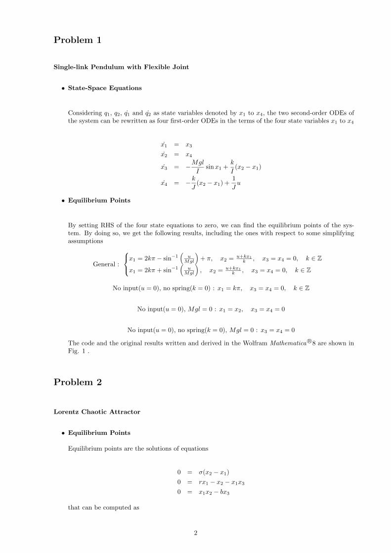
Considering q1, q2, q1 and q2 as state variables denoted by x1 to x4, the two second-order ODEs ofthe system can be rewritten as four first-order ODEs in the terms of the four state variables x1 to x4

x1 = x3

x2 = x4

x3 = −Mgl

Isinx1 +

k

I(x2 − x1)

x4 = − kJ

(x2 − x1) +1

Ju

• Equilibrium Points

By setting RHS of the four state equations to zero, we can find the equilibrium points of the sys-tem. By doing so, we get the following results, including the ones with respect to some simplifyingassumptions

General :

x1 = 2kπ − sin−1(

uMgl

)+ π, x2 = u+kx1

k , x3 = x4 = 0, k ∈ Z

x1 = 2kπ + sin−1(

uMgl

), x2 = u+kx1

k , x3 = x4 = 0, k ∈ Z

No input(u = 0), no spring(k = 0) : x1 = kπ, x3 = x4 = 0, k ∈ Z

No input(u = 0), Mgl = 0 : x1 = x2, x3 = x4 = 0

No input(u = 0), no spring(k = 0), Mgl = 0 : x3 = x4 = 0

The code and the original results written and derived in the Wolfram Mathematica R©8 are shown inFig. 1 .

Problem 2

Lorentz Chaotic Attractor


Equilibrium points are the solutions of equations

0 = σ(x2 − x1)

0 = rx1 − x2 − x1x30 = x1x2 − bx3

that can be computed as

2

Figure 1: The code used and results generated for problem 1

3

x?1 = 0 , x?2 =

√b√r − 1√b√r − 1

r − 1

, x?3 =

−√b√r − 1

−√b√r − 1

r − 1

.

• Linearization and Stability Discussion around the Origin

Jacobiab matrix of an autonomous nonlinear system with the state-space equation of the form

x = f(x)

is

J =∂f

∂x

which for a 3 × 3 system equals ∂f1∂x1

∂f1∂x2

∂f1∂x3

∂f2∂x1

∂f2∂x2

∂f2∂x3

∂f3∂x1

∂f3∂x2

∂f3∂x3

.

By substituting f1, f2 and f3 for

f1 = σ(x2 − x1)

f2 = rx1 − x2 − x1x3f3 = x1x2 − bx3

in f =

f1f2f3

and x for

x1x2x3

, the Jacobian would be

J(x) =

−σ σ 0r − x3 −1 −x1x2 x1 −b

which means we can rewrite the system state-space equations around the origin linear as

x = J(0)x

i.e.

x1 = σ(x2 − x1)

x2 = rx1 − x2x3 = −bx3 .

For determining the stability of the system around the origin, we have to figure out the sign of realparts of J(0) eigenvalues. Eigenvalues λi are the roots of the 3rd-order polynomial det(λI − J(0)).The three eigenvalues is computed to be

λ1 = −b

λ2 =1

2

(−σ − 1−

√4rσ + σ2 − 2σ + 1

)λ3 =

1

2

(−σ − 1 +

√4rσ + σ2 − 2σ + 1

).

The expression under the radicals, 4rσ+ (σ− 1)2, is positive for all positive values of σ and r, so theeigenvalues are always real. Therefore, for the system to be stable around origin, they themselvesmust be negative. These three simultaneous inequalities, i.e.

4

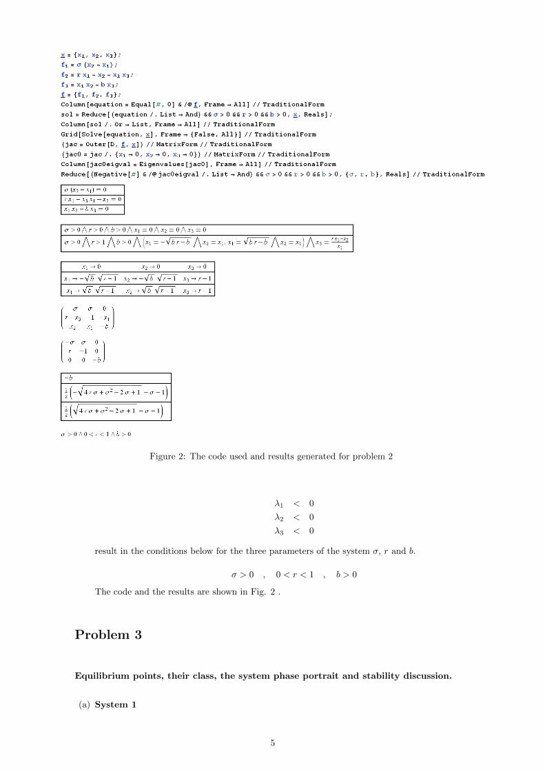
Figure 2: The code used and results generated for problem 2

λ1 < 0

λ2 < 0

λ3 < 0

result in the conditions below for the three parameters of the system σ, r and b.

σ > 0 , 0 < r < 1 , b > 0

The code and the results are shown in Fig. 2 .

Problem 3

Equilibrium points, their class, the system phase portrait and stability discussion.

(a) System 1

5

• Equilibrium Points{x1(1− x21) + x2 = 0

x2 = 0⇒ x?1 :

{x1 = −1

x2 = 0x?2 :

{x1 = 0

x2 = 0x?3 :

{x1 = 1

x2 = 0

• Equilibrium Classes

J(x) =

(1− 3x21 1

0 −1

)

J(x?1) =

(−2 10 −1

)⇒

{λ1 = −2

λ2 = −1⇒ Hyperbolic : Stable Node

J(x?2) =

(1 10 −1

)⇒

{λ1 = −1

λ2 = 1⇒ Hyperbolic : Saddle Point

J(x?3) =

(−2 10 −1

)⇒

{λ1 = −2

λ2 = −1⇒ Hyperbolic : Stable Node

• Linearization around Equilibrium Points

At the points x?1 and x?3 we can write

x1 = −2x1 + x2

x2 = −x2 .

Besides, the corresponding eigenvectors for λ1 and λ2 are

v1 =

(10

), v2 =

(11

).

Moreover, at the point x?2, the linearized equations of system are

x1 = x1 + x2

x2 = −x2 .

Similarly, the related eigenvectors can be calculated as

v1 =

(−12

), v2 =

(10

).

So the trajectories around these three equilibrium points, i.e. x?1, x?2 and x?3, including the cor-responding eigenvectors, can be sketched qualitatively as depicted in Fig. 3 . The code used isshown in Fig. 4 .

• Computer Computations

The code used and results generated for system (a) using Mathematica R©8 are shown in Fig.5. The results generated using MATLAB R© software are also shown in Fig. 6 . Separatix tra-jectories are sketched in both software. Stable Nodes and Saddle Points are marked with greenand red stars in Fig. 6, respectively.

(b) System 2

6

Figure 3: Trajectories around x?1, x?2 and x?3, respectively from left to right.

Figure 4: The code used to generate Fig. 3 diagrams.


Inspecting the equilibrium equations, i.e.

0 = −x2 + 2x1(x21 + x22)

0 = x1 + 2x2(x21 + x22)

we can see that there’s no equilibria other than origin, mostly because of the term x21 + x22. It’sobvious from the reverse side. For example, suppose that x 6= 0. Then if both x1 and x2 havethe same sign, the second equation won’t be satisfied. Otherwise, if they have different signs,the first equation will be unsatisfiable. So, x? = 0.


The Jacobian Matrix of the system equals

J =∂f

∂x=

(4x21 + 2(x21 + x22) 4x1x2 − 1

4x1x2 + 1 4x22 + 2(x21 + x22)

)which is evaluated at the origin to

J(0) =

(0 −11 0

).

Its eigenvalues are {λ1 = i

λ2 = −i

which are on the imaginary axis. So the equilibrium point is non-hyperbolic. But by evaluatingvector field f at many points x of a bounding box around the origin, the trajectories and con-sequently local stability around the origin can be determined qualitatively. This procedure and

7

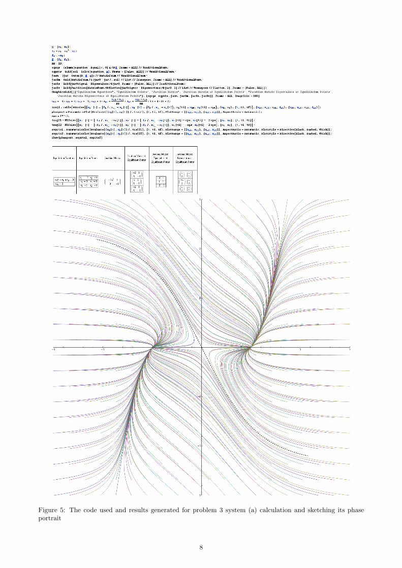
Figure 5: The code used and results generated for problem 3 system (a) calculation and sketching its phaseportrait

8

Figure 6: Phase Portrait for problem 3 system (a) using MATLAB software (left) & a closer look (right).

the used code and generated results are depicted in Fig. 7 .


Since the equilibria is non-hyperbolic, linearization doesn’t work in the case. The Jacobianeigenvectors are also as below

v1 =

(i1

), v2 =

(−i1

).

But again by inspecting the state-space equations, it seems that a polar coordinate transforma-tion may match to the problem. By doing so, substituting{

x1 = r cos θ

x2 = r sin θ

in the state-space equations, we can conclude that{r = 2r3

θ = 1,

which says r > 0 and θ > 0 that leads to going away of any trajectory from the origin, whilecounter-clockwise circulating around it. This is exactly the same result that could obviously beseen in Fig. 7 and means that it’s an unstable equilibrium, namely, Unstable Focus.


The code used for calculations of system (b) in Mathematica R©8 is shown in Fig. 8 . Theintegration for numerical ODE solving couldn’t be continued after approximately t = 0.03, be-cause of system having stiffness or singularity.

(c) System 3


Due to equilibrium equations

0 = cosx2

0 = sinx1

9

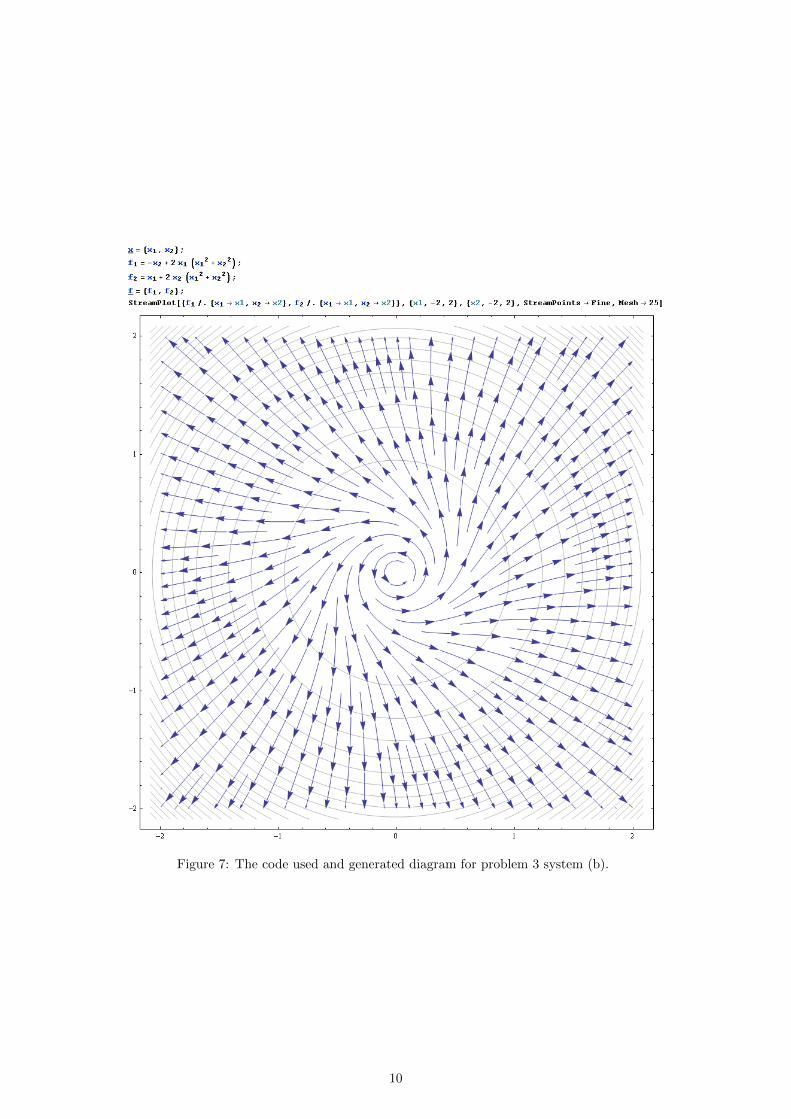
Figure 7: The code used and generated diagram for problem 3 system (b).

10

Figure 8: The code used and partial generated diagram for problem 3 system (b).

11

Figure 9: The code used and resulted trajectories in a sample region for problem 3 system (c).

Equilibrium Points are

x?1,k,l =

(2kπ

2lπ + π2

), x?2,k,l =

((2k + 1)π

(2l + 1)π + π2

), x?3,k,l =

(2kπ

(2l + 1)π + π2

), x?4,k,l =

((2k + 1)π2lπ + π

2

), k , l ∈ Z.


Jacobian Matrix is equal to

J =

(0 − sinx2

cosx1 0

),

evaluated at these four sets of equilibrium points, we have

J1 =

(0 −11 0

), J2 =

(0 1−1 0

), J3 =

(0 −1−1 0

), J4 =

(0 11 0

).

The corresponding eigenvalues are as below

forJ1 andJ2 :

{λ1 = i

λ2 = −iand forJ3 andJ4 :

{λ1 = 1

λ2 = −1.

The trajectories are sketched in a sample region containing some points of the first and some of

the second type, depicted in Fig. 9 .

(0π2

)from the first and

(0−π2

)from the second type are

completely visible in the sketch. As can be verified from the sketch, equilibrium points of thethird and fourth sets are Saddle Points and the ones of the first and second sets are Centres,though Centres are not definitely determined from the eigenvalues.


12

Figure 10: The code used and resulted trajectories around a Centre of problem 3 system (c).

Around the Saddle Points [with λ1,2 = ±1] we can write

forx?3,k,l :

{x1 = −x2x2 = −x1

and forx?4,k,l :

{x1 = x2

x2 = x1.

But around Centres (x?1,k,l and x?2,k,l) [with λ1,2 = ±i], linearization doesn’t mean. Trajectoriesaround those two sample points are depicted in more detail, individually in Fig. 10 and Fig. 11.


The results and the code for calculation and Phase Portrait sketching of the system (c) areshown in Fig. 12 , Fig. 13 and Fig. 14 . Again, Separatix trajectories are sketched in Fig. 12. Phase Portrait sketched also using MATLAB R© shown in Fig. 15 . Saddle Points and Centresare also marked with red and magenta stars in Fig. 15 , respectively.

(d) System 4



13

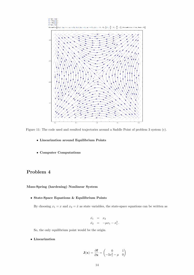
Figure 11: The code used and resulted trajectories around a Saddle Point of problem 3 system (c).



Problem 4

Mass-Spring (hardening) Nonlinear System

• State-Space Equations & Equilibrium Points

By choosing x1 = x and x2 = x as state variables, the state-space equations can be written as

x1 = x2

x2 = −µx1 − x31 .

So, the only equilibrium point would be the origin.

• Linearization

J(x) =∂f

∂x=

(0 1

−3x21 − µ 0

)

14

Figure 12: Calculations & Phase Portrait of problem 3 system (c).

15

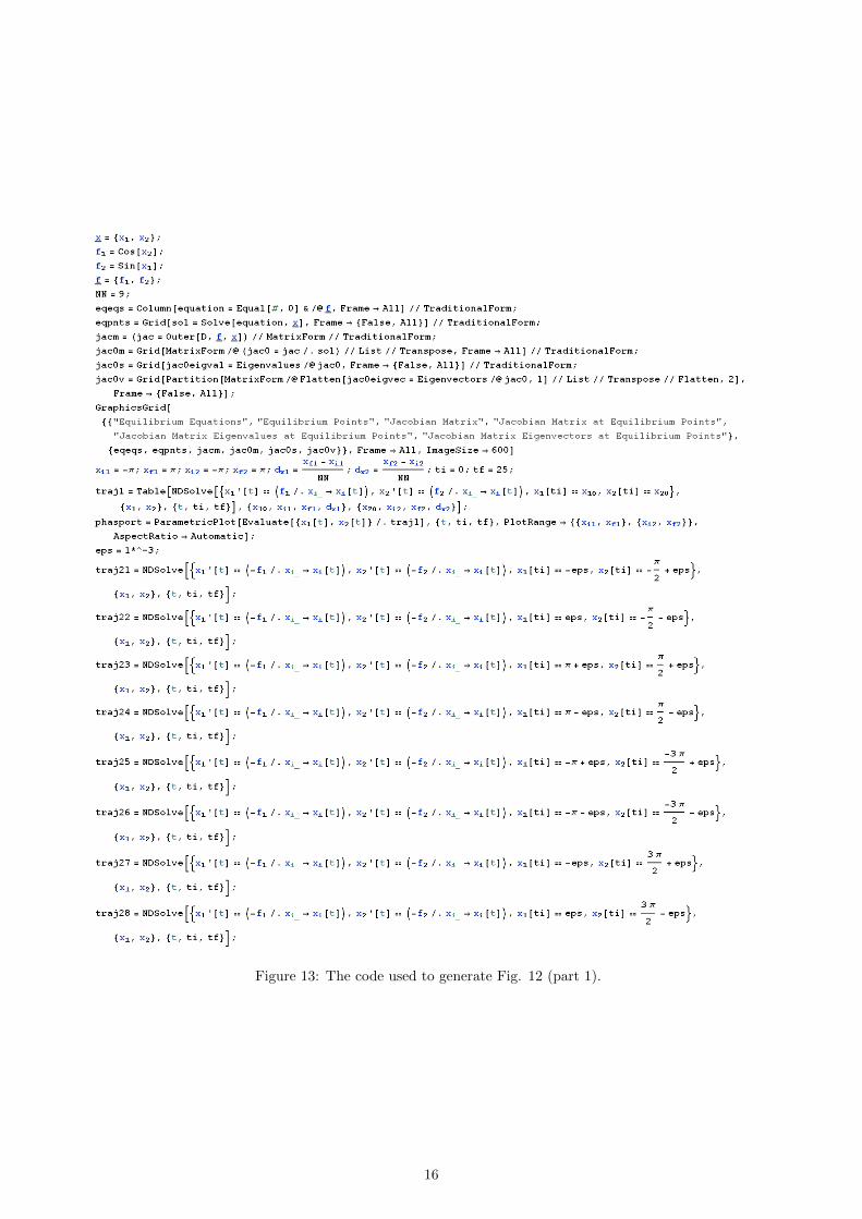
Figure 13: The code used to generate Fig. 12 (part 1).

16

Figure 14: The code used to generate Fig. 12 (part 2).

Figure 15: Phase Portrait of problem 3 system (c) using MATLAB R©

17

Figure 16: Problem 4 system trajectories around the origin for µ = 0 (top-left), µ = 0.1 (top-right), µ = 1(bottom-left) and µ = 10 (bottom-right).

J(0) =

(0 1−µ 0

), λ1 = −i√µ , λ2 = +i

√µ , v1 =

( +i√µ

1

), v2 =

( −i√µ

1

).

Equilibrium point (origin) is non-hyperbolic and so, linearization is impossible. Trajectories aroundthe origin for four different values of µ (µ = 0, 0.1, 1, 10) are sketched and depicted in Fig. 16 .


The code used and results generated for calculation and phase portrait sketching using Mathematica R©

is shown in Fig. 17 and Fig. 18 , respectively. Phase portrait using MATLAB R© are also shown inFig. 19 . Origin marked with a magenta star ia Centre.

Problem 5

Considering x as an n-dimensional vector denoting by(x1 x2 . . . xn

)Tand || · || as a k-norm defined by

||x||k =

(n∑i=1

|xi|k) 1k

.

Equilibrium equation states that

x(||x||2 − 1

)= 0.

Letting k = 2 for simplifying, the equilibrium points will be any of the two following situations,

18

Figure 17: Code used for calculation and sketching phase portrait of problem 4’s system (Fig. 18 ).

Figure 18: Calculations and phase portrait generated for system of problem 4 using Mathematica R©

19

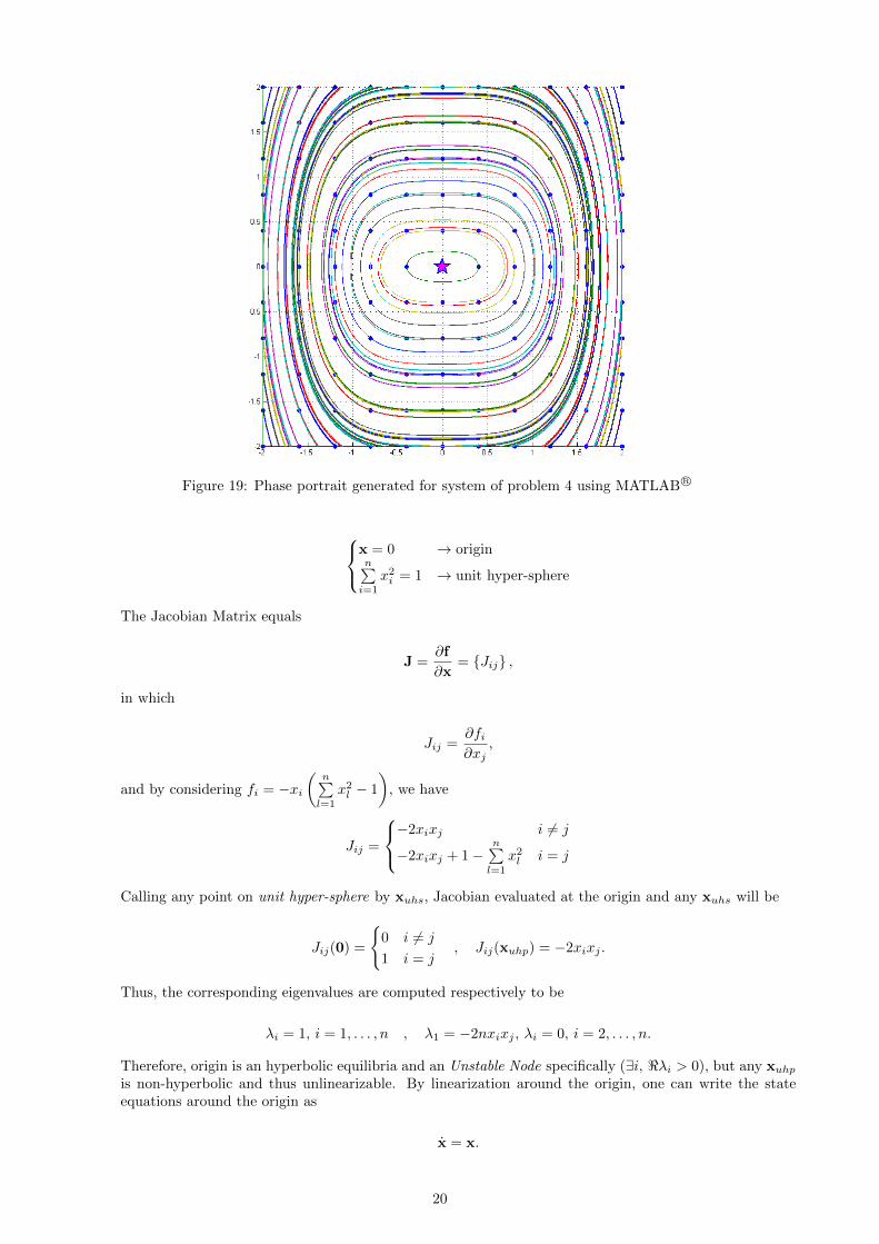
Figure 19: Phase portrait generated for system of problem 4 using MATLAB R©

x = 0 → originn∑i=1

x2i = 1 → unit hyper-sphere

The Jacobian Matrix equals

J =∂f

∂x= {Jij} ,

in which

Jij =∂fi∂xj

,

and by considering fi = −xi(

n∑l=1

x2l − 1

), we have

Jij =

−2xixj i 6= j

−2xixj + 1−n∑l=1

x2l i = j

Calling any point on unit hyper-sphere by xuhs, Jacobian evaluated at the origin and any xuhs will be

Jij(0) =

{0 i 6= j

1 i = j, Jij(xuhp) = −2xixj .

Thus, the corresponding eigenvalues are computed respectively to be

λi = 1, i = 1, . . . , n , λ1 = −2nxixj , λi = 0, i = 2, . . . , n.

Therefore, origin is an hyperbolic equilibria and an Unstable Node specifically (∃i, <λi > 0), but any xuhpis non-hyperbolic and thus unlinearizable. By linearization around the origin, one can write the stateequations around the origin as

x = x.

20

Sketching the 3D (n = 3) vector field f which is shown in Fig. 20 shows that the 3D sphere is a StableRegion which attracts points from inside or outside of the sphere. Unit sphere is plotted in transparentto see the vector field inside the sphere easily.

Problem 6

(a) By polar coordinate transformation {x1 = r cos θ

x2 = r sin θ

the equations can be rewritten in the form of

r = r3 − rθ = r2 − 1.

r vanishes at r = 0 and both r and θ do at r = 1. By sketching r and θ versus r, we can find outabout their signs. The two graphs are depicted in Fig. 21 . From these graphs, we can concludethat origin is an stable point, since r is negative in the vicinity of origin, in fact at all points locatedinside the unit disk (r < 1) except the origin itself. For points outside of the unit disk (r > 1),r > 0, which means that the trajectory is diverging from the origin and this shows the instability.Moreover, at the circle border, the trajectory changes the circulating direction around the origin, i.e.θ sign changes. All the points located on the unit circle are kind of equilibrium points of the system,because r = 0 and θ = 0. As a matter of fact, the system has Multiple Continuous EquilibriumPoints in (r, θ) domain.By considering the new equations, we can write

dr

dθ= r,

from which we can derive

r = rθθ00

which shows the exponential relation of r on θ where r0 = r(t0) and θ0 = θ(t0).

By sketching the vector field of the system, the phase portrait of the system can be qualitativelyunderstood, that is exactly the same as we conclude from equations in polar coordinates. The fieldis depicted in Fig. 22 . It can be seen that unit circle divides plane into two regions of inside andoutside of it. It’s also obvious from the negative real part of Jacobian eigenvalues (λ = −1 ± i)calculated and shown in Fig. 23 . The origin is a Stable Focus.

(b) The equilibrium equations states that

0 = −x1 − x20 = x1 − x32.

So, we must have

x1 = −x2x1 + x31 = 0.

Then, the only equilibrium point will be the origin. Sketching trajectories based on vector fieldmethod results in what is shown in Fig. 24 . It shows local stability of origin. The used code andresults for calculations and phase portrait sketching is shown in Fig. 25 . They show that origin is

a stable point and exactly a Stable Focus. It can also be seen from the eigenvalues (λ = −12 ± i

√32 )

calculated and shown in Fig. 25 .

21

Figure 20: Trajectories around origin of problem 5 system (n = 3).

Figure 21: r and θ for problem 6 system (a)

22

Figure 22: Phase Portrait and the code for system (a) of problem 6.

Figure 23: Code used and results for calculations of problem 6 system (a)

23

Figure 24: Trajectories around origin for system (b) of problem 6

24

Figure 25: The code and result for system (b) of problem 6

25

nonlinear control assignment #1 solutions - saba web …nonlinear control assignment #1 solutions...

Documents