nonlinear control and servo systems · nonlinear control and servo systems ... (see proof in...
TRANSCRIPT

Nonlinear Control and Servo Systems
Lecture 2
• Lyapunov theory cont’d.
• Storage function and dissipation
• Absolute stability
• The Kalman-Yakubovich-Popov lemma
• Circle Criterion
• Popov Criterion

Krasovskii’s method
Consider
x = f (x), f (0) = 0, f (x) ,= 0, ∀x ,= 0
and
A = f
x
If A+ AT < 0 ∀x ,= 0
then use V = f (x)T f (x) > 0, ∀x ,= 0,
V = f T f + f T f
=
f =
f
xx = A f
= f TA+ AT
f < 0, ∀x ,= 0
See more general case in [Khalil, Exercise 4.10 ]
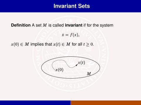
Invariant Sets
Definition A set M is called invariant if for the system
x = f (x),
x(0) ∈ M implies that x(t) ∈ M for all t ≥ 0.
x(0)
x(t)
M

Invariant Set Theorem
Theorem Let Ω ∈ Rn be a bounded and closed set that is
invariant with respect to
x = f (x).
Let V : Rn → R be a radially unbounded C1 function such that
V(x) ≤ 0 for x ∈ Ω. Let E be the set of points in Ω where
V(x) = 0. If M is the largest invariant set in E, then every
solution with x(0) ∈ Ω approaches M as t→∞ (see proof in
textbook)
Ω E M
V(x)E M x
Common use is to try to show that the origin is the larges invariant set of E, (M = 0).

Example – saturated control
Exercise - 5 min (revisited)
Find a bounded control signal u = sat(v), which globally
stabilizes the system
x1 = x1x2
x2 = u
u = sat (v(x1, x2))
(1)
Hint: Use the Lyapunov function candidate
V2 = ln(1+ x21) +α x22
for some appropriate value of α .

V2 = ln(1+ x21) +α x22/2
V2 = 2x1 x1
1+ x21
+ 2α x2 x2
= 2x2
x211+ x2
1︸ ︷︷ ︸0≤⋅⋅⋅<1
+α sat(v)
Can use some part to cancelx21
1+x21
and some to add bounded
negative damping in x2 (like sin(x2) or sat(x2) or ...)
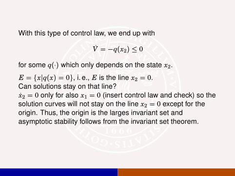
With this type of control law, we end up with
V = −q(x2) ≤ 0
for some q(⋅) which only depends on the state x2.
E = xpq(x) = 0, i. e., E is the line x2 = 0.Can solutions stay on that line?
x2 = 0 only for also x1 = 0 (insert control law and check) so the
solution curves will not stay on the line x2 = 0 except for the
origin. Thus, the origin is the larges invariant set and
asymptotic stability follows from the invariant set theorem.

Invariant sets - nonautonomous systems
Problems with invariant sets for nonautonomous systems.
V =V
t+V
xf (t, x) depends both on t and x.
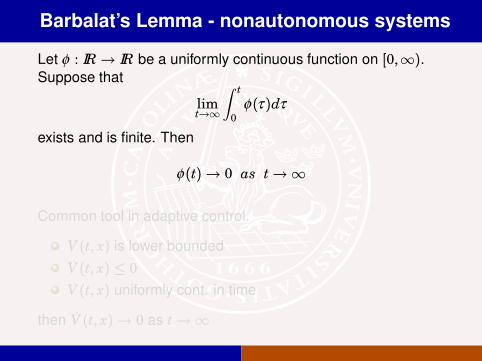
Barbalat’s Lemma - nonautonomous systems
Let φ : IR → IR be a uniformly continuous function on [0,∞).Suppose that
limt→∞
∫ t
0
φ(τ )dτ
exists and is finite. Then
φ(t) → 0 as t→∞
Common tool in adaptive control.
V (t, x) is lower bounded
V(t, x) ≤ 0
V(t, x) uniformly cont. in time
then V (t, x) → 0 as t→∞

Remark: In many adaptive control cases we have a Lyapunov
function candidate depending on states and parameter errors,
while the time-derivative of the candidate function only depends
on the states.

Nonautonomous systems —-cont’d
[Khalil, Theorem 4.8 & 4.9]
Assume there exists V (t, x) such that
W1(x) ≤︸ ︷︷ ︸positive definite
V (t, x) ≤ W2(x)︸ ︷︷ ︸decrecent
V (t, x) =V
t+V
xf (t, x) ≤ −W3(x)
W3 is a continuous positive semi-definite function.
Solutions to x = f (t, x) starting in x(t0) ∈ x ∈ Brp... are
bounded and satisfy
W3(x(t)) → 0 t→∞
See example in Khalil.

An instability result - Chetaev’s Theorem
Idea: show that a solution arbitrarily close to the origin have to
leave.
Let f (0) = 0 and let V : D → R be a continuously differentiable
function on a neighborhood D of x = 0, such that V (0) = 0.Suppose that the set
U = x ∈ D : qxq < r,V (x) > 0
is nonempty for every r > 0. If V > 0 in U , then x = 0 is
unstable.
V > 0
dV/dt > 0

Exercise - 5 min [Slotine]
Consider the system
x1 = x21 + x
32
x2 = −x2 + x31
Use Chetaev’s theorem to show that the origin is an unstable
equilibrium point.
You may consider
V = x1 − x22/2
for a certain region.

Dissipativity
Consider a nonlinear system
x(t) = f (x(t),u(t), t), t ≥ 0y(t) = h(x(t),u(t), t)
and a locally integrable function
r(t) = r(u(t), y(t), t).
The system is said to be dissipative with respect to the supply
rate r if there exists a storage function S(t, x) such that for all
t0, t1 and inputs u on [t0, t1]
S(t0, x(t0)) +
∫ t1t0
r(t)dt ≥ S(t1, x(t1)) ≥ 0
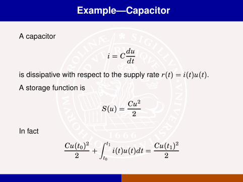
Example—Capacitor
A capacitor
i = Cdu
dt
is dissipative with respect to the supply rate r(t) = i(t)u(t).
A storage function is
S(u) =Cu2
2
In fact
Cu(t0)2
2+
∫ t1t0
i(t)u(t)dt =Cu(t1)
2
2

Example—Inductance
An inductance
u = Ldi
dt
is dissipative with respect to the supply rate r(t) = i(t)u(t).
A storage function is
S(i) =Li2
2
In fact
Li(t0)2
2+
∫ t1t0
i(t)u(t)dt =Li(t1)
2
2

Memoryless Nonlinearity
The memoryless nonlinearity w = φ(v, t) with sector condition
α ≤ φ(v, t)/v ≤ β , ∀t ≥ 0,v ,= 0
is dissipative with respect to the quadratic supply rate
r(t) = −[w(t) −α v(t)][w(t) − βv(t)]
with storage function
S(t, x) " 0

Linear System Dissipativity
The linear system
x(t) = Ax(t) + Bu(t), t ≥ 0
is dissipative with respect to the supply rate
−
[x
u
]TM
[x
u
]
and storage function xTPx if and only if
M +
[ATP+ PA PB
BTP 0
]≥ 0

Storage function as Lyapunov function
For a system without input, suppose that
r(y) ≤ −kpxpc
for some k > 0. Then the dissipation inequality implies
S(t0, x(t0)) −
∫ t1t0
kpx(t)pcdt ≥ S(t1, x(t1))
which is an integrated form of the Lyapunov inequality
d
dtS(t, x(t)) ≤ −kpxpc
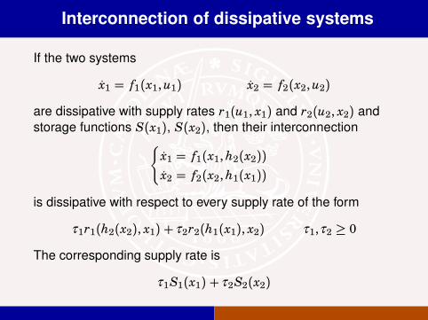
Interconnection of dissipative systems
If the two systems
x1 = f1(x1,u1) x2 = f2(x2,u2)
are dissipative with supply rates r1(u1, x1) and r2(u2, x2) and
storage functions S(x1), S(x2), then their interconnection
x1 = f1(x1,h2(x2))
x2 = f2(x2,h1(x1))
is dissipative with respect to every supply rate of the form
τ1r1(h2(x2), x1) + τ2r2(h1(x1), x2) τ1,τ2 ≥ 0
The corresponding supply rate is
τ1S1(x1) + τ2S2(x2)

Global Sector Condition
β
α
ψ
Let ψ (t, y) ∈ R be piecewise continuous in t ∈ [0,∞) and
locally Lipschitz in y ∈ R.
Assume that ψ satisfies the global sector condition
α ≤ψ (t, y)/y ≤ β , ∀t ≥ 0, y ,= 0 (2)
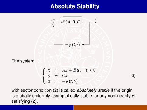
Absolute Stability
+
yu
replacements
Σ(A, B,C)
−ψ (t, ⋅)
The system
x = Ax + Bu, t ≥ 0y = Cx
u = −ψ (t, y)(3)
with sector condition (2) is called absolutely stable if the origin
is globally uniformly asymptotically stable for any nonlinearity ψsatisfying (2).

The Circle Criterion
−1/α −1/β
The system (3) with sector condition (2) is absolutely stable if
the origin is asymptotically stable for ψ (t, y) = α y and the
Nyquist plot
C( jω I − A)−1B + D, ω ∈ R
does not intersect the closed disc with diameter [−1/α ,−1/β ].
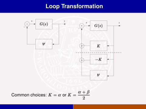
Loop Transformation
+
−
yu
+
+
+
−
yu
G(s)G(s)
ψ
ψK
−K
Common choices: K = α or K =α + β
2

Special Case: Positivity
Let M( jω ) = C( jω I − A)−1B + D, where A is Hurwitz. The
system
x = Ax + Bu, t ≥ 0y = Cx + Duu = −ψ (t, y)
with sector condition
ψ (t, y)/y ≥ 0 ∀t ≥ 0, y ,= 0
is absolutely stable if
M( jω ) +M( jω )∗ > 0, ∀ω ∈ [0,∞)
Note: For SISO systems this means that the Nyquist curve lies
strictly in the right half plane.

Proof
Set
V (x) = xTPx, P = PT > 0
[ V = 2xTPx
= 2xTP[A B
] [ x−ψ
]≤ 2xTP
[A B
] [ x−ψ
]+ 2ψ y
= 2[xT −ψ
] [P 0
0 I
] [A B
−C −D
] [x
−ψ
]
By the Kalman-Yakubovich-Popov Lemma, the inequality
M( jω ) + M( jω )∗ > 0 guarantees that P can be chosen to
make the upper bound for V strictly negative for all
(x,ψ ) ,= (0, 0).
Stability by Lyapunov’s theorem.

The Kalman-Yakubovich-Popov Lemma
Exists in numerous versions
Idea: Frequency dependence is replaced by matrix
equations/inequalities or vice versa 1
1Yakubovich in Lund: –"Yesterday, Ulf told me that nowadays we mostly
use it the other way round!”

The Kalman-Yakubovich-Popov Lemma
Exists in numerous versions
Idea: Frequency dependence is replaced by matrix
equations/inequalities or vice versa 1
1Yakubovich in Lund: –"Yesterday, Ulf told me that nowadays we mostly
use it the other way round!”

The K-Y-P Lemma, version I
Let M( jω ) = C( jω I − A)−1B + D, where A is Hurwitz. Then
the following statements are equivalent.
(i) M( jω ) + M( jω )∗ > 0 for all ω ∈ [0,∞)
(ii) ∃P = PT > 0 such that
[P 0
0 I
] [A B
C D
]+
[A B
C D
]T [P 0
0 I
]< 0
Compare Khalil (5.10-12):
M is strictly positive real if and only if ∃P,W, L, ǫ :[PA+ ATP PB − CT
BTP− C D + DT
]= −
[ǫP+ LTL LTW
WTL WTW
]
——————————————
Mini-version a la [ Slotine& Li ]:
x = Ax + bu, A Hurwitz, (i. e., Reλ i(A) < 0]
y = cx
The following statements are equivalent
Rec( jω I − A)−1b > 0,∀w ∈ [0,∞)
There exist P = PT > 0 and Q = QT > 0 such that
ATP+ PA = −Q
Pb = cT

The K-Y-P Lemma, version II
For
[Φ(s)Φ(s)
]=
[C
C
](sA− A)−1(B − sB) +
[D
D
],
with sA− A nonsingular for some s ∈ C, the following two
statements are equivalent.

The K-Y-P Lemma, version II - cont.
(i) Φ( jω )∗Φ( jω ) + Φ( jω )∗Φ( jω ) ≤ 0 for all ω ∈ R
with det( jω A − A) ,= 0.
(ii) There exists a nonzero pair (p, P) ∈ R$Rn$n
such that p ≥ 0, P = P∗ and
[A B
C D
]∗ [P 0
0 pI
][A B
C D
]
+
[A B
C D
]∗ [P 0
0 pI
] [A B
C D
]≤ 0
The corresponding equivalence for strict inequalities holds with
p = 1.
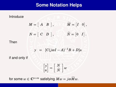
Some Notation Helps
Introduce
M =[A B
], M =
[I 0
],
N =[C D
], N =
[0 I
].
Then
y = [C( jω I − A)−1B + D]u
if and only if
[y
u
]=
[N
N
]w
for some w ∈ Cn+m satisfying Mw= jω Mw.

Lemma 1
Given y, z∈ Cn, there exists an ω ∈ [0,∞) such that y = jω z, if
and only if yz∗ + zy∗ = 0.
Proof Necessity is obvious. For sufficiency, assume that
yz∗ + zy∗ = 0. Then
pv∗(y+ z)p2 − pv∗(y− z)p2 = 2v∗(yz∗ + zy∗)v = 0.
Hence y = λ z for some λ ∈ C ∪ ∞. The equality
yz∗ + zy∗ = 0 gives that λ is purely imaginary.

Proof of the K-Y-P Lemma
See handout (Rantzer)

(i) and (ii) can be connected by the following sequence of
equivalent statements.
(a) w∗(N∗N + N∗N)w < 0 for w ,= 0 satisfying
Mw= jω Mw with ω ∈ R.
(b) Θ ∩P = ∅, where
Θ =(w∗(N∗N + N∗N)w, Mww∗M ∗ +Mww∗M ∗
):
w∗w = 1
P = (r, 0) : r > 0
(c) (convΘ) ∩P = ∅.
(d) There exists a hyperplane in R$Rn$n separating
Θ from P , i.e. ∃P such that ∀w ,= 0
0 > w∗(N∗N + N∗N + M ∗PM + M ∗PM
)w
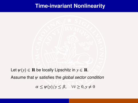
Time-invariant Nonlinearity
Let ψ (y) ∈ R be locally Lipschitz in y ∈ R.
Assume that ψ satisfies the global sector condition
α ≤ψ (y)/y ≤ β , ∀t ≥ 0, y ,= 0

The Popov Criterion
v
βv
ψ (v)
−2 0 2 4 6 8 10 12 14−12
−10
−8
−6
−4
−2
0
2
ω ImG(iω )
ReG(iω )
− 1β
Suppose that ψ : R→ R is Lipschitz and 0 ≤ψ (v)/v ≤ β . Let
G(iω ) = C(iω I − A)−1B with A Hurwitz and (A,B,C) minimal.
If there exists η ∈ R such that
Re [(1+ iωη)G(iω )] > −1
βω ∈ R (4)
then the differential equation x(t) = Ax(t) − Bψ (Cx(t)) is
exponentially stable.

Popov proof I
Set
V (x) = xTPx + 2ηβ
∫ Cx
0
ψ (σ )dσ
where P is an n$ n positive definite matrix. Then
V = 2(xTP +ηkψ C)x
= 2(xTP +ηβψ C)[A B
] [ x−ψ
]
≤ 2(xTP +ηβψ C)[A B
] [ x−ψ
]− 2ψ (ψ − β y)
= 2[xT −ψ
] [ PA PB
−βC−ηβCA −1−ηβCB
] [x
−ψ
]
By the K-Y-P Lemma there is a P that makes the upper bound
for V strictly negative for all (x,ψ ) ,= (0, 0).
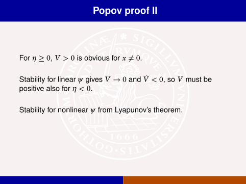
Popov proof II
For η ≥ 0, V > 0 is obvious for x ,= 0.
Stability for linear ψ gives V → 0 and V < 0, so V must be
positive also for η < 0.
Stability for nonlinear ψ from Lyapunov’s theorem.

The Kalman-Yakubovich-Popov lemma – III
Given A ∈ Rn$n, B ∈ Rn$m, M = MT ∈ R(n+m)$(n+m), with
iω I − A nonsingular for ω ∈ R and (A, B) controllable, the
following two statements are equivalent.
(i)
[(iω I − A)−1B
I
]∗
M
[(iω I − A)−1B
I
]≤ 0 ∀ω ∈
(ii) There exists a matrix P ∈ Rn$n such that P = P∗
and
M +
[ATP+ PA PB
BTP 0
]≤ 0

Proof techniques
(ii) [(i) simple
Multiply from right and left by
[(iω I − A)−1B
I
]
(i) [(ii) difficult
Spectral factorization (Anderson)
Linear quadratic optimization (Yakubovich)
Find (1, P) as separating hyperplane between the sets
([x
u
]TM
[x
u
], x(Ax + Bu)∗ + (Ax + Bu)x∗
): (x,u) ∈ Cn+m
(r, 0) : r ≥ 0

1