Nonlinear Capital Taxation

Iván Werning, MIT

June 8, 2010 (9:20am)

Preliminary and Incomplete

do not circulate

Abstract

This paper studies tax design in a dynamic Mirrleesian economy, where agents face

labor productivity shocks that are private information. I characerize a system of non-

linear taxes on savings that implement any incentive compatible allocation. I restrict

the savings tax to be independent of the current state. The tax schedule is differen-

tiable under quite general conditions and its derivative, the marginal tax, coincides

with the wedge in the agent’s intertemporal Euler equation. Although I allow for

nonlinear schedules, a linear tax often suffices. Otherwise, the tax can always be made

convex—in this sense, progressive taxation is always feasible. Finally, I show how the

savings tax can be made independent of the history of shocks.

1

1 Introduction

When insurance is imperfect, individuals may wish to smooth their consumption by sav-

ing and dissaving a riskless asset. However, if insurance is limited because of asymmetric

information, it may be best to restrict free access to savings, since optimal incentive com-

patible allocations may not be attainable otherwise [Rogerson, 1985]. Some distortion

must be introduced in savings choices to achieve constrained-efficient allocations. In dy-

namic Mirrleesian models, featuring privately observed labor productivity shocks, this

leads to the possibility that capital taxation may be desirable (Diamond and Mirrlees,

1978; Golosov et al., 2003; Kocherlakota, 2005). The question I address here is the precise

form of such a distortionary tax system.

Of course, one possibility is to ban individuals from saving altogether. Such a tax

system would essentially replicate the direct mechanism used in the revelation principle,

which controls consumption directly. Less extreme alternatives seem more palatable. At a

practical level, they are more comparable to actual or potential tax policy. On a theoretical

level, they can be more revealing, as when marginal tax rates make explicit the distortions

that are implicit in the allocation.

Kocherlakota [2005] and Albanesi and Sleet [2006] provide alternative tax systems that

are less extreme than direct mechanisms. Kocherlakota studied a tax system where wealth

is taxed linearly, with a tax rate that varies with the past history of shocks as well as with

the current shock. The dependence on the current shock is crucial. It ensures that saving

is never optimal for the agent regardless of the reporting strategy. Albanesi and Sleet

study a model with i.i.d. shocks and provide an implementation where wealth is taxed

jointly with current labor income in a nonlinear way. In both these implementations, the

dependence of the wealth tax on the current shock makes the after-tax rate of return faced

by agents risky.

The goal of this paper is to offer a new implementation with some desirable features.

I study tax systems that allow the savings tax to be nonlinear but require it to be inde-

pendent of the current shock. Thus, the after-tax rate of return faced by agents is riskfree.

I show that the tax schedule can be made differentiable quite generally. The marginal

tax rate then coincides with the intertemporal wedge in the standard consumption Euler

equation.1 Interestingly, although the tax schedule is allowed to be nonlinear, I show that

a linear tax suffices in some cases. Otherwise, the tax schedule can always be made con-

vex. Thus, progressive taxation, in the sense of increasing marginal tax rates, is always

1The intertemporal wedge is defined, for any given allocation, as the proportional adjustment in the rateof return on capital that is required for the standard consumption Euler equation, i.e. letting Uc,t denotemarginal utility at time t the wedge τt is such that Uc,t = β(1 + rt)(1 − τt)Et[Uc,t+1].

2

feasible. Finally, I show two ways of removing history dependence in the savings tax.

These results do not require utility to be separable in consumption and labor. All of these

features contrast quite sharply with previous implementations.

Some well-known examples in the literature seem directly at odds with my results.

These examples have motivated the need for state-dependent savings taxes, that is, for

conditioning on the current shock or labor income. For instance, Kocherlakota [2004,

2005] shows that if the savings tax is differentiable and state-independent, then the agent

may plan on a “double deviation”: saving some positive amount and reporting a lower

shock in the next period. In the example, productivity types are discrete and the optimal

allocation has the agent indifferent between reporting truthfully and misreporting to be

the productivity type immediately below. When the agent is allowed to save, any small

amount of positive savings breaks this indifference in favor of misreporting. Similarly,

although a savings tax may discourage savings under the truth-telling strategy, saving

some positive amount is strictly optimal under a misreporting strategy. As a result, the

double deviation is always desirable and the intended implementation fails. These ex-

amples allow one to conclude that optimal allocations, discrete shocks, differentiable tax

functions and state-independent taxes are incompatible. Kocherlakota relaxes the latter

assumption and proceeds to characterize state-dependent taxes.

This paper takes a different route. I show that a nonlinear tax schedule allows for

an implementation without conditioning on the current shock. I do not rule out kinks a

priori, only to show that kinks are mostly unnecessary. Indeed, the tax schedule can be

made differentiable quite generally.

Before moving on, it is important to understand that kinks are inherently natural with

finite shocks to productivity. Even in the static Mirrlees [1971] model, kinks in the labor-

income tax are optimal in this case (see Section 3).2 It is only natural to expect the same for

the savings tax in dynamic extensions. In that case, it seems inconsistent to insist on the

differentiability of the savings tax, but allow for kinks in the labor-income tax. At a more

fundamental level, it seems onerous to expect a model to yield smooth solutions, such as

differentiable tax schedules, when primitives, such as the distribution of productivity, are

not assumed continuous.

In any case, I show that kinks are unnecessary under plausible conditions. In partic-

ular, the savings tax schedule can be made differentiable when productivity shocks are

continuously distributed. The “double deviation” example, discussed above, had a finite

2In Mirrlees (1971), kinks may be required in the income-tax schedule even when the distribution ofproductivity is continuous if bunching is optimal over some interval of productivities. Unlike those due tothe assumption of finite shocks, these kinks have no counterpart in the savings tax schedule I characterize.

3

number of shocks. I show that this assumption is not innocuous: when shocks are con-

tinuously distributed, double deviations cease to be a problem. To understand this, recall

that indifference was crucial for the desirability of double deviations. But with a con-

tinuous distribution of shocks, indifference is a knife-edge phenomena that occurs with

probability zero.

Moreover, even with finite productivity shocks, kinks are unimportant. First of all,

for a finite but large number of productivity shocks, I show that the kinks required to

implement the optimal allocation are minimal. That is, they shrink and vanish (with

left and right derivatives converge to each other) as the number of shocks is expanded.

More importantly, even when the number of productivity types is small, differentiable tax

schedules can implement allocations that come arbitrarily close to optimal ones. In fact,

the closure of the set of allocations achievable by differentiable tax schedules is the full

set of incentive compatible allocations. Thus, essentially no welfare is lost by insisting on

differentiable tax schedules.

Although I allow the savings tax to be nonlinear, I show that in some cases a linear

one suffices. The logic for this is as follows. Suppose a tax schedule induces some agent

to choose a certain level of savings. Now, replace this schedule with one that is tangent to

it at that savings level and above it everywhere else. The agent will continue to find the

same level of savings optimal, so this new tax schedule implements the same allocation.

In this sense, the tax schedule is not unique, only the marginal tax rate is pinned down.

In particular, any concave tax schedule can be replaced by its linear tangent. Thus, the

question is whether the desired allocation can be implemented by a concave tax schedule.

I show that this is the case whenever the agent’s value function is concave in wealth, or,

equivalently, when consumption rises with wealth. Numerical explorations for a set of

standard distributions of skills and preferences always find that this is the case. I conclude

that although a nonlinear tax is generally required to remove the dependence of the tax

on the current state, a linear tax will work in important cases.

The same tangency principle explains why the tax schedule can always be made strictly

convex. In this sense, progressive taxation of savings, with rising marginal tax rates, is

always feasible.

Finally, I explore the possibility of making the savings tax history independent. It is

important to understand that most allocations, including optimal ones, will feature in-

tertemporal wedges that are history dependent. Thus, the challenge is to create a savings

tax that is history independent yet manages to deliver the appropriate history-dependent

wedges.3

3Studying the subset of allocations and welfare that obtain using relatively simple and history-

4

I show that this can be done in two ways. The first implementation has agents saving

in a history independent manner. The history independent schedule is set as the upper

envelope of the history dependent ones. As long as the intertemporal wedge varies across

histories this upper envelope schedule will feature a kink at the equilibrium savings point.

Indeed, the left and right derivatives are precisely the smallest and largest intertemporal

wedge, respectively.

The second way of making the savings tax history independent avoids generating

kinks. In the model, individual savings and tax transfers are indeterminate due to stan-

dard Ricardian equivalence arguments. Unlike previous implementations, this one relies

on agents saving in a history dependent manner. The idea is to have wealth be a sufficient

statistic for the desired intertemporal wedge. Different wealth positions then place agents

on different points of the history independent schedule, precisely where the marginal tax

rate equals the desired intertemporal wedge.

A simple and attractive feature of my implementation is that, if an incentive-compatible

allocation is obtained by allowing agents to save freely, then this arrangement belongs to

the set studied here. In other words, the tax systems I consider would include the one that

generated the allocation in the first place. In contrast, the implementation in Kocherlakota

[2005] would yield non-zero and stochastic taxes for such an allocation.4

It is virtually impossible to judge implementations objectively. They are all just as

good within the logic of the model—including the direct mechanism. Unspecified con-

siderations may guide us, but until those are made explicit it remains a subjective exercise.

In the meantime, it seems useful to understand many possible tax systems, studying their

properties, the choices they offer agents, the informational requirements they place on the

tax agency, and the like. The main contribution of this paper should be seen as an effort

in this direction.

The rest of the paper is organized as follows. I begin by deriving the implementation

for a two-period economy in Section 2. I then take up the differentiability of the sav-

ings tax schedule in Section 3, considering both the case with a continuous distribution

and that with finite shocks. In Section 4 I extend the implementation to longer horizons.

Section 5 explores how to make the savings tax history independent.

independent tax systems (including the tax on savings and income) is an interesting different questionthat is not attempted here. The goal here, as stated at the outset of the paper, remains to implement anyincentive compatible allocation, not a subset. The goal now is to attempt this with a history-independentsavings tax, but allowing the labor-income tax to remain history dependent.

4One cannot ask the same question for the implementation in Albanesi and Sleet [2006], since theirresults only apply to optimal allocations (which feature savings distortions).

5

2 Two Period Horizon

It is useful to begin with a two-period horizon. Section 4 extends the implementation to

longer horizons.

Time periods are denoted t = 0, 1. Productivity is given by θt. Initial productivity, θ0,

is known, while θ1 is uncertain. It is realized privately to the agent at t = 1. An allocation

specifies c0, y0, c1(θ1), y1(θ1) and delivers utility

v∗0 = U0(c0, y0, θ0) + βE[

U1(

c1(θ1), y1(θ1), θ1

)]

,

where Ut(c, y, θ) represents the utility in period t = 0, 1, assumed to be increasing in c and

θ, concave in (c, y) and satisfy the standard single-crossing condition that the marginal

rates of substitution Utc(c, y, θ)/Ut

y(c, y, θ) is increasing in θ, for any given (c, y).

Unlike Kocherlakota [2005] and Albanesi and Sleet [2006], the implementation I de-

velop does not require additively separable utility of the form U(c, y, θ) = u(c) − h(y, θ).

Theoretically, the additively separable case is an important benchmark since it is required

for the Inverse Euler characterization of constrained optimal allocations. Empirically,

Aguiar and Hurst [2005] provide evidence supporting departures from separability in

the direction of assuming that consumption (expenditures) c and labor y are Hicksian

complements, so that Ucy > 0.

Incentive compatibility requires truth telling to be optimal

U1(

c1(θ1), y1(θ1), θ1

)

≥ U1(

c1(r1), y1(r1), θ1

)

for all θ1 ∈ Θ and all r1 ∈ Θ; here, r1 represents the report made by the agent regarding

the true shock θ1.

This concludes the description of the model’s environment. The main goal of this

paper is to extend a given mechanism so that it allows for saving and attains the same

equilibrium allocation. For that purpose, it is unnecessary to introduce technology, or to

set up a planning problem and solve for optimal allocations.

6

2.1 Nonlinear Tax Implementation

For any given incentive compatible allocation (c0, y0, c1(θ1), y1(θ1)), consider an imple-

mentation that confronts the agent with the following budget constraints:

c̃0 + a1 ≤ c0,

c̃1 ≤ R(a1) + c1(r1).

Here where R(·) represents the retention function, with R(0) = 0. If the net interest rate

is r then R(a) − (1 + r)a represents a nonlinear tax on wealth at t = 1.

Without loss of generality, one can take R to be increasing. Equivalently, consider the

budget constraints

c̃0 + M(x1) ≤ c0,

c̃1 ≤ x1 + c1(r1),

for M = R−1, with M(0) = 0. If the net interest rate is r then M(x)− x/(1 + r) represents

a nonlinear savings tax at t = 0. Clearly, one can go back and forth between R and M. I

shall use the second formulation and refer to M as the savings tax function.

These budget constraints strictly augment the original direct mechanism by adding a

saving choice x1; the constraints effectively specialize to the direct mechanism when x1 =

0. The agent takes M as given and optimizes by choosing a saving and reporting strategy.

The tax function M is said to implement the proposed allocation (c0, y0, c1(θ1), y1(θ1)) if

the agent finds it optimal to save zero x1 = 0. The original incentive compatibility of the

allocation then ensures that truth telling is optimal.

Consider the agent’s problem in two stages. In the second period, the agent enters

holding wealth x1, then productivity θ1 is realized and the agent makes a report r1. The

utility obtained is

V1(x1, θ1) ≡ maxr1

U1(

c1(r1) + x1, y1(r1), θ1

)

.

Define the set of maximizers to be

R∗(x1, θ1) ≡ arg maxr1

U1(

c1(r1) + x1, y1(r1), θ1

)

Given a choice of x1, expected utility is

W0(x1; M) ≡ U0(

c0 − M(x1), y0, θ0

)

+ βE[V1(x1, θ1)].

7

Suppose the allocation is incentive compatible so that W0(0; M) = v∗0 if M(0) = 0. Now

define M∗(x) so that

W0(x1; M) = v∗ ∀x1.

Solving for the tax schedule M gives

M∗(x1) ≡ c0 − Ψ0(

v∗ − βE[V1(x1, θ1)], y0, θ0

)

, (1)

where Ψt(·, y, θ) denotes the inverse of Ut(·, y, θ). Of course, since this construction im-

plies indifference, if taxes are set higher than M∗ for x1 6= 0, then x1 = 0 remains optimal

for the agent. Conversely, any tax schedule below M∗ offers a better expected welfare

opportunity than v∗ and cannot implement the desired allocation. I summarize these

arguments in the following proposition.

Proposition 1. Any incentive compatible allocation is implemented for any M(x1) ≥ M∗(x1)

with M(0) = M∗(0) = 0, where M∗(x1) is defined by equation (1).

The tax schedule M∗ is the lowest tax that implements any given allocation. It does

so by making the agent indifferent to saving any quanitity. Tax schedules are not unique,

since higher taxes for x 6= 0 help discourage saving x1 6= 0 further.

In the next two sections I study the shape of tax functions M satisfying Proposition

1. I start with the local property of differentiability. Since M∗ is a lower envelope, it

contains important local information about any feasible schedule M. In particular, if M

is differentiable at x = 0 then its derivative, the marginal tax, must coincide with that of

M∗. Indeed, it turns out that, M can be differentiable at x = 0 only if the same is true for

M∗. I turn to investigate conditions for the latter.

3 Differentiability: Marginal Taxes and Wedges

For any allocation, define m∗ to be the marginal rate of substitution by

U0c (c0, y0, θ0)m∗ ≡ βE

[

U1c

(

c1(θ1), y1(θ1), θ1

)]

.

So that m∗ corresponds to the shadow price that makes the agent’s standard intertemporal

Euler equation hold. If the interest rate is r, then

m∗ −1

1 + r

8

is a measure of the distortion implicit in the allocation. This is sometimes termed the

intertemporal wedge or implict marginal tax rate.

When M∗(x1) is differentiable at x1 = 0. The first order condition for the agent implies

that the marginal tax should equal the M∗′(0) = m∗. Thus, in my implementation the

marginal tax equals the intertemporal wedge. That is, implicit and explicit marginal tax

rates coincide. I now investigate conditions for differentiability.

3.1 Left and Right Derivatives

The key to establishing differentiability properties for M∗ is to verify the differentiability

of V1(·, θ1). Envelope theorems can be used for this, since V1 is defined by a maximization.

In particular, Corollary 4 in Milgrom and Segal [2002] applies in our case and implies that

V1(·, θ1) is left- and right-differentiable and that are given by

∂

∂x1V1(x1+, θ1) = max

r∈R∗(x1,θ1)U1

c (c1(r) + x̃1, y1(r), θ1)

∂

∂x1V1(x1−, θ1) = min

r∈R∗(x1,θ1)U1

c (c1(r) + x̃1, y1(r), θ1)

respectively. Thus, kinks can only occur where R∗(x1, θ1) is not unique. These represent

situations where the agent is indifferent to two or more reports r1.

Note that∂

∂x1V1(x1−, θ1) ≤

∂

∂x1V1(x1+, θ1)

so that only convex, but not concave, kinks are possible. It also follows that

M∗′(x1−) ≤ m∗ ≤ M∗′(x1+).

Next I investigate when these inequalities can be assured to hold with equality.

3.2 Continuous Distribution of Shocks

I now show that the tax schedule M∗(x1) is differentiable if the distribution of productiv-

ity is continuous. The idea is that indifference of the agent with respect to the report, is

a “knife edge” phenomena. From an ex-ante perspective, when productivity is continu-

ously distributed, indifference occurs with probability zero. It follows that V1 is almost

everywhere differentiable and that E[V1(·, θ1)] is differentiable.

Proposition 2. If θ1 is continuously distributed then M∗(x1) defined by equation (1) is differen-

9

tiable and M∗′(0) = m∗.

Proof. Incentive compatibility implies that c1(θ1) and y1(θ1) are non-decreasing functions

of θ1. It follows that there are at most countably many points of discontinuity. Define Θ̂ to

be the set of points of discontinuity in c1(·). By Theorem 3 in Milgrom and Segal (2002),

the function V1(x1, θ1) is differentiable with respect to x1 at x1 = 0 and θ1 /∈ Θ̂, with

derivative given by the envelope formula: Vx(0, θ1) = U1c (c1(θ1), y1(θ1), θ1) (since r1 = θ1

is optimal by incentive compatibility). The function of interest to us is

V1(x1) ≡ E[V(x1, θ1)],

the integral of a function that is differentiable at x1 = 0 except on a set of countable

points. With a continuous distribution for θ1 the set of points of non-differentiability is of

probability zero. It then follows that V(x1) is differentiable at x1 = 0 with derivative

V ′1(0) = E

[

Vx(0, θ1)]

= E[

U1c

(

c1(θ1), y1(θ1), θ1

)]

.

In other words, if the net interest rate is r, the marginal tax rate M′(0) − 1/(1 + r)

exists and coincides with the intertemporal wedge in the Euler equation.

3.3 Finite Shocks

If productivity types are finite, so that Θ = {θ1, θ2, . . . , θN}, then indifference may occur

with positive probability, produces a convex kink: M∗′(0−) < M∗′(0+). Indeed, this will

typically be the case at optimal allocations, because downward incentive constraints bind.

I first show that, with finite types, kinks occur in the labor income tax schedule. Thus,

they are not limited to the savings tax, but inherent to the Mirrlees [1971] model.

With finite types, incentive constraints bind downward at an optimal allocation, so

that

v1(θn) ≡ U1(

c1(θn), y1(θn), θn)

= U1(

c1(θn−1), y1(θn−1), θn)

∀n = 2, . . . , N.

In addition, output is non-decreasing, so that y1(θn−1) ≤ y1(θn) for n = 2, . . . , N. Fol-

lowing Mirrlees [1971], one seeks an incodme tax schedule T(Y), defined for all Y ≥ 0, so

that agents face the budget constraint

c1 ≤ y1 − T(y1)

10

in the second period. Ensuring that agents choose the original allocation requires

U1(

Y − T(Y), Y, θn)

≤ v1(θn)

for all Y ≥ 0, with equality at Y = y(θn) for n = 1, . . . , N. This is equivalent to

T(Y) ≥ T∗(Y) ∀Y

T(Y) = T∗(Y) ∀Y = y(θn) for n = 1, . . . , N.

where

T∗(Y) ≡ maxn

{Y − Ψ1[v1(θn), Y, θn)]}.

Note that T∗ is differentiable whenever the maximization over n that defines it is unique.

Conversely, whenever the maximum is attained by more than one n then the function T∗

has a convex kink. This is precisely what happens, at y(θn) for n = 1, . . . N − 1 when

downward incentive constraint are binding. I summarize this observation in a proposi-

tion.

Proposition 3. Suppose the set of productivity types is finite. Any income tax schedule T :

R+ → R that implements the optimal allocation cannot be differentiable at points Y = y(θn) for

n = 1, . . . , N − 1. Moreover, if T has left and right derivatives at any of these points then there

must be a convex kink: T′(Y−) < T′(Y+).

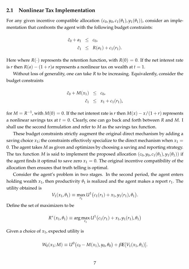
The situation is illustrated in Figure 1 for the case with two shocks. In conclusion,

with finite types, kinks are pervasive at the optimum. They occur both for labor-income

taxes as well as the savings tax.

Nevertheless, two ideas suggest that kinks due to finite shocks should be of little con-

cern.

First, if incentive constraints bind, one can perturb the allocation so that they are slack.

In this way, one can come arbitrarily close to any desired allocation, and its welfare, with

a differentiable tax function.

Proposition 4. Suppose shocks are finite Θ = {θ1, θ2, . . . , θN}. Take any incentive compatible

allocation c0, y0, c1(θ1), y1(θ1). Then for any ε > 0 there exists differentiable tax functions Mε

and Tε that implement allocations (cε0, yε

0, cε1(θ1), yε

1(θ1)) so that |cε0 − c0| < ε, |yε

0 − y0| < ε,

|cε1(θ1)− c1(θ1)| < ε and |yε

1(θ1)− y1(θ1)| < ε.

It is also possible to add a technological constraint for the allocations (cε0, yε

0, cε1(θ1),

yε1(θ1)) to be feasible.

11

y

c

(yL, cL)

(yH , cH)

θL

θH

Figure 1: An example with two types Θ = {θL, θH} where the incentive constraint for θH

initially binds. A small increase in savings x > 0 makes the indifference curves steeper,and reporting L optimal for both agent types, θL and θH , becomes optimal.

Second, I conjecture that the size of this kink disappears as the number of shocks is

increased N → ∞ so that Θ becomes dense in some interval [θ, θ̄]. As the grid points are

expanded the distance between any two types shrinks and the probability at any one type

vanishes. As a result, for large N most agents will be indifferent to a consumption-labor

bundle very close to their own; only a vanishing fraction may be indifferent to a more

distant point. For small but positive savings x1 > 0 agents underreport, but the deviation

in consumption and labor is small and vanishing. As a result, the left and right derivative

in the envelope formula approach each other.

4 Linear and Progressive Capital Taxation

Interestingly, although I allow for nonlinear taxation, in some cases a linear tax will do. To

see this, recall that Proposition 1 states that any function M(x1) ≥ M∗(x1) will implement

the desired allocation. It follows that, whenever M∗(x1) is concave that one can set M(x1)

to be a linear function that acts as a supporting tangent at x1 = 0. Inspection of equation

12

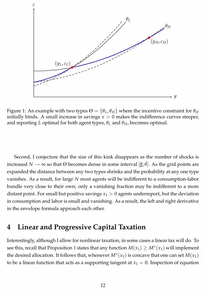
y

M∗(x)

M∗L,L(x)

M∗L,H(x)0

Figure 2: An example with two types Here M∗L,H(x) and M∗

L,L(x) respectively representthe tax functions required for a truth telling strategy and a strategy that always reportsthe low shock. That is, M∗

L,H(x1) = c0 − Ψ0(

v∗ − βE[U1(

c1(θ1) + x1, y1(θ1), θ1

)

], y0, θ0

)

and M∗L,L(x) = c0 − Ψ0

(

v∗ − βE[U1(

c1(θL) + x1, y1(θL), θ1

)

], y0, θ0

)

.

(1) shows that this will be the case if E[V1(·, θ1)] is concave.5 A sufficient condition for

this is for each V1(·, θ1) function to be concave, for all θ1 ∈ Θ. Of course, this condition is

not necessary: E[V1(·, θ1)] may be if V(·, θ1) is only concave for a subset of values of θ1.

Concavity of V1(x1) is not a foregone conclusion. A sufficient condition for concavity

is that the agent faces as a convex tax schedule in the second period, so that the the loci of

points (y, c) available to him are in a convex relation. This will be the case if labor-income

taxation is progressive.

Proposition 5. (a) If V1(x1) is concave a linear schedule M(x1) = (1 + τ)x1 implements the

optimal allocation with x1 = 0. (b) If labor income taxation is progressive in period t = 1, then

V1(x1) is concave.

5This follows by the following fact. Suppose f : R → R is decreasing and concave and that g : R → R

is decreasing and convex Then f (g(·)) is concave. Start with the fact that f is concave to deduce:

α f (g(x1)) + (1 − α) f (g(x2)) ≤ f (αg(x1) + (1 − α)g(x2)).

Now, by convexity of g,αg(x1) + (1 − α)g(x2) ≥ g(αx1 + (1 − α)x2).

Since f is decreasing it follows that

f (αg(x1) + (1 − α)g(x2)) ≤ f (g(αx1 + (1 − α)x2)).

Putting the first and last inequality together yields the desired result.

13

y

c

(yL, cL)

(yH , cH)

θL

θH

(y′L, c′L)

Figure 3: A smooth tax function can be created by shifting the allocation for θL so thatthe incentive constraints are slack. The lower envelope (in blue) represents the retentionfunction Y − T(Y).

5 Arbitrary Finite Horizon

Now suppose there are periods t = 0, 1, . . . , T. The agent has utility function

T

∑t=0

βtE[Ut(ct, yt, θt)]. (2)

Assume {θt} is a Markov process with θt ∈ Θ.

Consider any incentive compatible allocation (c(θt), y(θt)) with equilibrium values

v(θt) satisfying

v(θt) = Ut(

c(θt), y(θt), θt

)

+ βE[v(θt+1)|θt]. (3)

The agent’s optimization problem has the Bellman equation

w(rt−1, θt) = maxrt

{

Ut(

c(rt), y(rt), θt

)

+ βE[w(rt, θt+1)|θt]}

. (4)

Here the agent enters a period having reported rt−1 in the past and learns his true shock

θt; thus, the state variable is (rt−1, θt). The agent then decides what report to make rt.6

6The Markov assumption allows us to ignore the history of shocks θt−1. Also, for an incentive compatibleallocation, truth telling is optimal even if the agent has made false reports in the past.

14

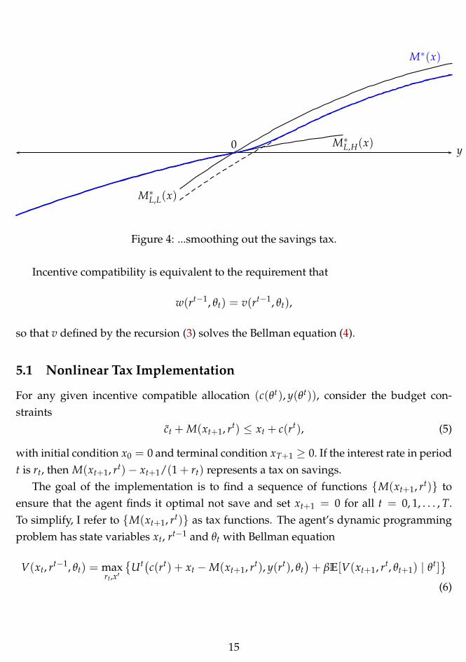
y

M∗(x)

M∗L,L(x)

M∗L,H(x)0

Figure 4: ...smoothing out the savings tax.

Incentive compatibility is equivalent to the requirement that

w(rt−1, θt) = v(rt−1, θt),

so that v defined by the recursion (3) solves the Bellman equation (4).

5.1 Nonlinear Tax Implementation

For any given incentive compatible allocation (c(θt), y(θt)), consider the budget con-

straints

c̃t + M(xt+1, rt) ≤ xt + c(rt), (5)

with initial condition x0 = 0 and terminal condition xT+1 ≥ 0. If the interest rate in period

t is rt, then M(xt+1, rt)− xt+1/(1 + rt) represents a tax on savings.

The goal of the implementation is to find a sequence of functions {M(xt+1, rt)} to

ensure that the agent finds it optimal not save and set xt+1 = 0 for all t = 0, 1, . . . , T.

To simplify, I refer to {M(xt+1, rt)} as tax functions. The agent’s dynamic programming

problem has state variables xt, rt−1 and θt with Bellman equation

V(xt, rt−1, θt) = maxrt,x′

{

Ut(

c(rt) + xt − M(xt+1, rt), y(rt), θt

)

+ βE[V(xt+1, rt, θt+1) | θt]}

(6)

15

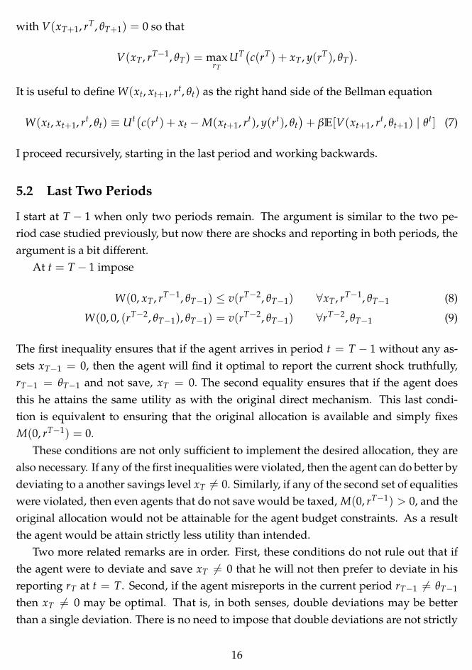
with V(xT+1, rT, θT+1) = 0 so that

V(xT, rT−1, θT) = maxrT

UT(

c(rT) + xT, y(rT), θT

)

.

It is useful to define W(xt, xt+1, rt, θt) as the right hand side of the Bellman equation

W(xt, xt+1, rt, θt) ≡ Ut(

c(rt) + xt − M(xt+1, rt), y(rt), θt

)

+ βE[V(xt+1, rt, θt+1) | θt] (7)

I proceed recursively, starting in the last period and working backwards.

5.2 Last Two Periods

I start at T − 1 when only two periods remain. The argument is similar to the two pe-

riod case studied previously, but now there are shocks and reporting in both periods, the

argument is a bit different.

At t = T − 1 impose

W(0, xT, rT−1, θT−1) ≤ v(rT−2, θT−1) ∀xT, rT−1, θT−1 (8)

W(0, 0, (rT−2, θT−1), θT−1) = v(rT−2, θT−1) ∀rT−2, θT−1 (9)

The first inequality ensures that if the agent arrives in period t = T − 1 without any as-

sets xT−1 = 0, then the agent will find it optimal to report the current shock truthfully,

rT−1 = θT−1 and not save, xT = 0. The second equality ensures that if the agent does

this he attains the same utility as with the original direct mechanism. This last condi-

tion is equivalent to ensuring that the original allocation is available and simply fixes

M(0, rT−1) = 0.

These conditions are not only sufficient to implement the desired allocation, they are

also necessary. If any of the first inequalities were violated, then the agent can do better by

deviating to a another savings level xT 6= 0. Similarly, if any of the second set of equalities

were violated, then even agents that do not save would be taxed, M(0, rT−1) > 0, and the

original allocation would not be attainable for the agent budget constraints. As a result

the agent would be attain strictly less utility than intended.

Two more related remarks are in order. First, these conditions do not rule out that if

the agent were to deviate and save xT 6= 0 that he will not then prefer to deviate in his

reporting rT at t = T. Second, if the agent misreports in the current period rT−1 6= θT−1

then xT 6= 0 may be optimal. That is, in both senses, double deviations may be better

than a single deviation. There is no need to impose that double deviations are not strictly

16

better than single deviations. What the conditions ensure is that no deviations are better

than any set of deviations.

The inequalities are equivalent to imposing that

M(xT , rT−1) ≥ M∗(xT, rT−1) (10)

where M∗ is the upper envelope over θT−1,

M∗(xT, rT−1) ≡ maxθT−1

M̃∗(xT, rT−1, θT−1), (11)

of the function

M̃∗(xT , rT−1, θT−1) ≡ c(rT−1)

− ΨT−1[

v(rT−2, θT−1)− βE[V(xT , rT−1, θT) | θT−1], y(rT−1), θT−1

]

. (12)

Intuitively, M̃∗ represents a fictitious tax function that would ensure that agents are in-

different to any savings and report, so that inequality (8) holds with equality for all xT,

rT−1 and θT−1. Such a tax function is not feasible, since it must depend on the true type

θT−1 in addition to the reports rT−1. Taking the upper envelope over true types θT−1 to

define M∗ yields a tax function that depends only on reports rT−1, while ensuring that the

inequality (8) continues to hold. Because one takes the upper envelope over θT−1, agents

confronted with M∗ will not typically be indifferent among several saving and reporting

strategies.

Conversely, M∗ is the lowest possible tax function that prevents a deviation from

xT−1 = 0, since any lower tax function would necessarily violates inequality (8) for some

type θT−1. Thus, the set of all feasible tax functions M are those that lie above M∗, satis-

fying inequality (10).

Finally, note that for each rT−1 and θT−1 the fictitious tax M̃∗ is exactly akin to the tax

function defined in equation (1) for the previous two-period horizon case, where it was

assumed that θT−1 = θ0 was known. The innovation here, when this last assumption is

dropped, is to take the upper envelope over θT−1 and to condition on the history rT−1.

The new construction rules out misreporting in period T − 1, as well as in period T.

17

5.3 Other Periods

I now work backward inductively defining a tax schedule for all periods t = 0, 1, . . . T − 1.

Suppose tax schedules for periods s = t + 1, t + 2, . . . , T − 1 have already been con-

structed. Associated with these tax schedules {M(xs+1, rs)}T−1s=t+1 are value functions

{V(xs, rs−1, θs)}T−1s=t+1. I seek to construct a tax schedule M(xt+1, rt) and value function

V(xt, rt−1, θt) for period t.

Recall that these functions W(xt, xt+1, rt, θt) are given by (7) using next period’s value

function V(xt+1, rt, θt+1) and the current tax schedule M(xt+1, rt), which must be con-

structed. I impose that, whatever the value function V(xt+1, rt, θt+1), that the tax function

M(xt+1, rt) be such that the implied W satisfy

W(0, xt+1, rt, θt) ≤ v(rt−1, θt) ∀xt+1, rt, θt (13)

W(0, 0, (rt−1, θt), θt) = v(rt−1, θt) ∀rt−1, θt (14)

These conditions are exactly analogous to the ones presented above. The previous condi-

tions (8)–(9) are the special case of conditions (13)–(14) for t = T − 1. Thus, the induction

argument could begin at T − 1 directly with the general arguments laid out in this subsec-

tion; however, the previous subsection was included for presentation purposes as warm

up to the more general ideas.

The reasons for imposing these conditions are the same as before. They ensure that in

period t the agent will find truth telling and no savings, rt = θt and xt+1 = 0 optimal, ob-

taining the same allocation and utility as the original allocation. They are both necessary

and sufficient for this.

The same arguments lead us to define

M∗(xt+1, rt, θt) ≡ c(rt)− Ψt[

v(rt−1, θt)− βE[V(xt+1, rt, θt+1) | θt], y(rt), θt

]

and

M∗(xt+1, rt) ≡ maxθt

M∗(xt+1, rt, θt), (15)

and set M(xt+1, rt) to be any function above this:

M(xt+1, rt) ≥ M∗(xt+1, rt). (16)

Given such a choice for M(xt+1, rt) this then defines a value function V(xt, rt−1, θt) using

the Bellman equation (6).

Continuing this way gives a tax schedule M(xt+1, rt) and value function V(xt, rt−1, θt)

18

for t = 0, 1, . . . , T − 1. This construction ensures that the Bellman equation (6) holds with

the maximum is attained by truth-telling and no savings, for all t = 0, 1, . . . , T − 1. By

the principle of optimality this implies that truth telling and no savings solves the agent’s

problem of maximizing (2) among all possible reporting and savings strategies satisfying

the budget constraint (5). This proves the following.

Proposition 6. Any incentive-compatible allocation {c(θt), y(θt)}Tt=0 can be implemented us-

ing the budget constraints (5) by any sequence tax functions on savings {M(xt+1, rt)}T−1t=0 sat-

isfying the inequalities (16), where M∗(xt+1, rt) defined implicitly from {M(xt+1, rt)}T−1t=0 us-

ing conditions (15) and the Bellman equation (6). Conversely, if a sequence of tax functions

{M(xt+1, rt)}T−1t=0 implements the incentive-compatible allocation {c(θt), y(θt)}T

t=0 it must sat-

isfy inequalities (16).

This construction creates all feasible tax schedules that implement the desired allo-

cation. Note that the tax schedules {M(xs+1, rt)}T−1s=t+1 chosen to satisfy (15)–(16) affect

the lowest tax schedule possible, M∗(xt+1, rt), in period t given by (15) and, thus, af-

fect the available tax schedule choices for period t satisfying (16). Indeed, higher choices

for the functions {M(xs+1, rt)}T−1s=t+1 lead to lower values of V(xt+1, rt, θt+1) and hence

lower values for M∗(xt+1, rt), i.e. more choices for M(xt+1, rt). In particular, because

of this decreasing relation between future and current tax schedules, it would be incor-

rect to interpret the sequence generated by always setting M(xt+1, rt) = M∗(xt+1, rt) for

t = 0, . . . , T − 1 as the lowest possible tax schedules (this is only the case for period T − 1).

Relatedly, seeking the lowest tax functions {M(xt+1, rt)}T−1t=0 is not a well-posed problem,

outside the two-period horizon. Nevertheless, the important point is that the characteri-

zation provided by (15)–(16) is exhaustive, providing all the tax schedules that implement

the allocation.

It is interesting to note how the tax schedules are dependent on each other. In other

words, constructing the tax schedules for one period cannot be done independently from

other periods. Similarly, the set of feasible tax schedule for period t depends on the entire

allocation for periods t, t + 1, . . . , T. This is unlike the implementation in Kocherlakota

[2005], which employs state-dependent linear taxes on capital; there, only the consump-

tion allocation in periods t and t + 1 is needed to compute tax rates at t + 1. In the present

case, however, the entire allocation is only relevant for the global nonlinear properties of

the tax schedules. As I show next, the marginal tax rates always equal the intertemporal

wedge, which can also be computed from the consumption allocation at t and t + 1.

19

x

M̄(x)

M(x; r′′)

M(x; r′)

M(x; r)0

Figure 5: A kinked upper envelope M̄(x) function constructed from M(x; r) functionsthat have not been transposed.

6 History Independent Taxation

Finally, I explore the possibility of making the savings tax history independent. It is

important to understand that most allocations, including optimal ones, will feature in-

tertemporal wedges that are history dependent. Thus, the challenge is to create a savings

tax that is history independent yet manages to deliver the appropriate history-dependent

wedges.

I show that this can be done in two ways. The first implementation has agents saving

in a history independent manner. The history independent schedule is set as the upper

envelope of the history dependent ones. As long as the intertemporal wedge varies across

histories this upper envelope schedule will feature a kink at the equilibrium savings point.

Indeed, the left and right derivatives are precisely the smallest and largest intertemporal

wedge, respectively.

The second way of making the savings tax history independent avoids generating

kinks. In the model, individual savings and tax transfers are indeterminate due to stan-

dard Ricardian equivalence arguments. Unlike previous implementations, this one relies

on agents saving in a history dependent manner. The idea is to have wealth be a sufficient

statistic for the desired intertemporal wedge. Different wealth positions then place agents

on different points of the history independent schedule, precisely where the marginal tax

20

x

M̄(x)

M(x; r′′)

M(x; r′)

M(x; r)

0

Figure 6: A smooth upper envelope M̄(x) function constructed from transposed M(x; r)functions.

rate equals the desired intertemporal wedge.

[to be completed]

References

Mark Aguiar and Erik Hurst. Consumption versus expenditure. Journal of Political Econ-

omy, 113(5):919–948, October 2005.

Stefania Albanesi and Christoper Sleet. Dynamic optimal taxation with private informa-

tion. Review of Economic Studies, 2006. forthcoming.

Peter A. Diamond and James A. Mirrlees. A model of social insurance with variable

retirement. Journal of Public Economics, 10(3), 1978.

Mikhail Golosov, Narayana Kocherlakota, and Aleh Tsyvinski. Optimal indirect and cap-

ital taxation. Review of Economic Studies, 70(3):569–587, 2003.

Narayana R. Kocherlakota. Figuring out the impact of hidden savings on optimal unem-

ployment insurance. Review of Economic Dynamics, 7:541–554, 2004.

21

x

M̄(x)

M(x; r′′)

M(x; r′)

M(x; r)

0

Figure 7: A smooth upper envelope M̄(x) function constructed from transposed M(x; r)functions.

Narayana R. Kocherlakota. Zero expected wealth taxes: A mirrlees approach to dynamic

optimal taxation. Econometrica, 73(5):1587–1621, 2005.

Paul Milgrom and Ilya Segal. Envelope theorems for arbitrary choice sets. Econometrica,

70(2):583–601, March 2002.

James A. Mirrlees. An exploration in the theory of optimum income taxation. Review of

Economic Studies, 38(2):175–208, 1971.

William P. Rogerson. Repeated moral hazard. Econometrica, 53(1):69–76, 1985.

22