nonlinear analysis and performance based design methods for
TRANSCRIPT

Nonlinear Analysis and Performance Based Design Methodsfor Reinforced Concrete Coupled Shear Walls
Danya S. Mohr
A thesis submitted in partial fulfillmentof the requirements for the degree of
Master of Science in Civil Engineering
University of Washington
2007
Program Authorized to Offer Degree: Civil & Environmental Engineering


University of WashingtonGraduate School
This is to certify that I have examined this copy of a master’s thesis by
Danya S. Mohr
and have found that it is complete and satisfactory in all respects,and that any and all revisions required by the final
examining committee have been made.
Committee Members:
Laura Lowes
Dawn Lehman
Greg Miller
Date:


In presenting this thesis in partial fulfillment of the requirements for a master’s degree atthe University of Washington, I agree that the Library shall make its copies freely availablefor inspection. I further agree that extensive copying of this thesis is allowable only forscholarly purposes, consistent with “fair use” as prescribed in the U.S. Copyright Law. Anyother reproduction for any purpose or by any means shall not be allowed without my writtenpermission.
Signature
Date


University of Washington
Abstract
Nonlinear Analysis and Performance Based Design Methodsfor Reinforced Concrete Coupled Shear Walls
Danya S. Mohr
Co-Chairs of the Supervisory Committee:Professor Laura Lowes
Department of Civil and Environmental Engineering
Professor Dawn LehmanDepartment of Civil and Environmental Engineering
Recent advances in structural engineering have lead to an increased interest in performance-
based design of structural systems. Here the performance of reinforced concrete coupled
wall systems, designed in accordance with current practice, is investigated.
Current design methods, including the plastic-design method recommended by the IBC
Structural/Seismic Design Manual (2007) were employed to design a 10-story reference
coupled wall for use in the study.
Linear and nonlinear analysis were conducted to assess the expected performance of
the reference coupled wall. Linear elastic modeling was done using SAP2000 (2006), while
nonlinear analysis were conducted using VecTor2 (2006). Nonlinear finite element models
and analysis methods were validated against a set of experimental coupling beam tests.
Additionally, the effects of confinement reinforcement on diagonally reinforced coupling
beams designed per the current ACI 318-05 code versus the proposed full confinement
method of the 318-08 code were investigated.
The results of these analysis suggest that current design methods can lead to coupled
shear walls that may not behave as desired in a significant seismic event.

TABLE OF CONTENTS
Page
List of Figures . . . . . . . . . . . . . . . . . . . . . . . . . . . . . . . . . . . . . . . . v
List of Tables . . . . . . . . . . . . . . . . . . . . . . . . . . . . . . . . . . . . . . . . . xiii
Glossary . . . . . . . . . . . . . . . . . . . . . . . . . . . . . . . . . . . . . . . . . . . . xv
Chapter 1: Introduction . . . . . . . . . . . . . . . . . . . . . . . . . . . . . . . . . 1
1.1 Objectives . . . . . . . . . . . . . . . . . . . . . . . . . . . . . . . . . . . . . . 2
1.2 Outline of Thesis . . . . . . . . . . . . . . . . . . . . . . . . . . . . . . . . . . 2
Chapter 2: Background Research . . . . . . . . . . . . . . . . . . . . . . . . . . . . 4
2.1 Building Inventory . . . . . . . . . . . . . . . . . . . . . . . . . . . . . . . . . 4
2.2 Coupling Beams . . . . . . . . . . . . . . . . . . . . . . . . . . . . . . . . . . 4
2.3 Previous Experimental Coupling Beam Studies . . . . . . . . . . . . . . . . . 8
2.3.1 Galano & Vignoli . . . . . . . . . . . . . . . . . . . . . . . . . . . . . . 9
2.3.2 Kwan & Zhao . . . . . . . . . . . . . . . . . . . . . . . . . . . . . . . . 9
2.3.3 Tassios, Maretti, and Bezas . . . . . . . . . . . . . . . . . . . . . . . . 10
2.3.4 Compiled Experiment Coupling Beam Data . . . . . . . . . . . . . . . 13
2.4 Previous Analyses . . . . . . . . . . . . . . . . . . . . . . . . . . . . . . . . . 21
2.4.1 Oyen . . . . . . . . . . . . . . . . . . . . . . . . . . . . . . . . . . . . . 21
2.4.2 Brown . . . . . . . . . . . . . . . . . . . . . . . . . . . . . . . . . . . . 21
2.4.3 Zhao et. al. . . . . . . . . . . . . . . . . . . . . . . . . . . . . . . . . . 21
Chapter 3: Coupling Beam Performance and Damage Patterns . . . . . . . . . . . 24
3.1 Behavior Mode Definition . . . . . . . . . . . . . . . . . . . . . . . . . . . . . 24
3.2 Experimental Behavior Modes . . . . . . . . . . . . . . . . . . . . . . . . . . . 25
3.3 Comparison Plots . . . . . . . . . . . . . . . . . . . . . . . . . . . . . . . . . . 33
i

Chapter 4: Nonlinear Finite Element Analysis of Coupling Beam Experiments . . 42
4.1 VecTor2 . . . . . . . . . . . . . . . . . . . . . . . . . . . . . . . . . . . . . . . 42
4.2 Modeling Decisions . . . . . . . . . . . . . . . . . . . . . . . . . . . . . . . . . 43
4.2.1 Material Properties . . . . . . . . . . . . . . . . . . . . . . . . . . . . . 43
4.2.2 Constitutive Models . . . . . . . . . . . . . . . . . . . . . . . . . . . . 43
4.2.3 Element Mesh . . . . . . . . . . . . . . . . . . . . . . . . . . . . . . . 45
4.2.4 Types of Reinforcement . . . . . . . . . . . . . . . . . . . . . . . . . . 48
4.2.5 Boundary Conditions . . . . . . . . . . . . . . . . . . . . . . . . . . . 49
4.2.6 Loading Parameters . . . . . . . . . . . . . . . . . . . . . . . . . . . . 49
4.3 Description of Evaluation Method . . . . . . . . . . . . . . . . . . . . . . . . 49
4.4 Reduced Data Set for Illustration of VecTor2 Capabilities . . . . . . . . . . . 55
4.5 Description of Results . . . . . . . . . . . . . . . . . . . . . . . . . . . . . . . 55
4.5.1 Galano P01 . . . . . . . . . . . . . . . . . . . . . . . . . . . . . . . . . 55
4.5.2 Galano P02 . . . . . . . . . . . . . . . . . . . . . . . . . . . . . . . . . 57
4.5.3 Tasssios CB2B . . . . . . . . . . . . . . . . . . . . . . . . . . . . . . . 58
4.6 Data Analysis and Trends . . . . . . . . . . . . . . . . . . . . . . . . . . . . . 68
4.7 Discussion and Comparison of Results . . . . . . . . . . . . . . . . . . . . . . 89
4.8 Model Parameter Study . . . . . . . . . . . . . . . . . . . . . . . . . . . . . . 90
4.8.1 Vecchio and Palermo Parameters . . . . . . . . . . . . . . . . . . . . . 90
Chapter 5: Evaluation of Transverse Reinforcement of Coupling Beams . . . . . . 92
5.1 Introduction . . . . . . . . . . . . . . . . . . . . . . . . . . . . . . . . . . . . . 92
5.1.1 Approach . . . . . . . . . . . . . . . . . . . . . . . . . . . . . . . . . . 92
5.1.2 Organization of Chapter . . . . . . . . . . . . . . . . . . . . . . . . . . 93
5.2 Design Requirements . . . . . . . . . . . . . . . . . . . . . . . . . . . . . . . . 93
5.2.1 ACI 318-05 Current Code . . . . . . . . . . . . . . . . . . . . . . . . . 93
5.2.2 ACI 318H-CH047d Proposal . . . . . . . . . . . . . . . . . . . . . . . . 94
5.3 Description of Models . . . . . . . . . . . . . . . . . . . . . . . . . . . . . . . 94
5.3.1 CBR-ACI: ACI318-05 Reference Model . . . . . . . . . . . . . . . . . 95
5.3.2 CBR-ACI-S: Reference model with additional slab steel . . . . . . . . 95
5.3.3 CBR-318H: Confinement to meet the ACI 318H proposal . . . . . . . 95
5.3.4 CBR-318H-F: Confinement of the entire section to meet ACI 318Hproposal . . . . . . . . . . . . . . . . . . . . . . . . . . . . . . . . . . . 96
ii

5.3.5 CBR-318H-M: Confinement of the entire section with reduced trans.reinf. . . . . . . . . . . . . . . . . . . . . . . . . . . . . . . . . . . . . . 96
5.4 Finite Element Modeling . . . . . . . . . . . . . . . . . . . . . . . . . . . . . . 965.5 Description of Evaluation Method . . . . . . . . . . . . . . . . . . . . . . . . 975.6 Simulation Results . . . . . . . . . . . . . . . . . . . . . . . . . . . . . . . . . 98
5.6.1 Load Drift Plots . . . . . . . . . . . . . . . . . . . . . . . . . . . . . . 985.6.2 Stiffness . . . . . . . . . . . . . . . . . . . . . . . . . . . . . . . . . . . 1045.6.3 Shear Force . . . . . . . . . . . . . . . . . . . . . . . . . . . . . . . . . 1055.6.4 Displacement and Drift . . . . . . . . . . . . . . . . . . . . . . . . . . 108
5.7 Comparison of Confinement Variations . . . . . . . . . . . . . . . . . . . . . . 1105.7.1 CBR-ACI vs. CBR-318H . . . . . . . . . . . . . . . . . . . . . . . . . 1105.7.2 CBR-ACI vs CBR-318H-F . . . . . . . . . . . . . . . . . . . . . . . . . 1125.7.3 CBR-ACI and CBR-318H-M . . . . . . . . . . . . . . . . . . . . . . . 115
5.8 Conclusions . . . . . . . . . . . . . . . . . . . . . . . . . . . . . . . . . . . . . 115
Chapter 6: Coupled Wall Design and Analysis . . . . . . . . . . . . . . . . . . . . 1196.1 Objective . . . . . . . . . . . . . . . . . . . . . . . . . . . . . . . . . . . . . . 1196.2 Current Design Methods Background . . . . . . . . . . . . . . . . . . . . . . . 119
6.2.1 Code Design . . . . . . . . . . . . . . . . . . . . . . . . . . . . . . . . 1196.2.2 2006 IBC Structural/Seismic Design Recommendations . . . . . . . . 120
6.3 Design of Coupled Wall Specimen . . . . . . . . . . . . . . . . . . . . . . . . . 1226.4 Strength Design . . . . . . . . . . . . . . . . . . . . . . . . . . . . . . . . . . . 1246.5 Recommended Plastic Design . . . . . . . . . . . . . . . . . . . . . . . . . . . 1276.6 Coupling Beam Reinforcement Details . . . . . . . . . . . . . . . . . . . . . . 1296.7 Coupled Wall Model Variations . . . . . . . . . . . . . . . . . . . . . . . . . . 1316.8 Modeling Decisions . . . . . . . . . . . . . . . . . . . . . . . . . . . . . . . . . 134
6.8.1 Constitutive Models . . . . . . . . . . . . . . . . . . . . . . . . . . . . 1346.8.2 Element Mesh . . . . . . . . . . . . . . . . . . . . . . . . . . . . . . . 1346.8.3 Reinforcement Model . . . . . . . . . . . . . . . . . . . . . . . . . . . 1386.8.4 Boundary Conditions . . . . . . . . . . . . . . . . . . . . . . . . . . . 1386.8.5 Loading Parameters . . . . . . . . . . . . . . . . . . . . . . . . . . . . 1386.8.6 Summary of Coupled Wall Model Variations . . . . . . . . . . . . . . 141
6.9 Description of Evaluation Method . . . . . . . . . . . . . . . . . . . . . . . . 1436.10 Displacement Control Results . . . . . . . . . . . . . . . . . . . . . . . . . . . 144
iii

6.11 Load Control Results . . . . . . . . . . . . . . . . . . . . . . . . . . . . . . . . 1466.11.1 Deformed Shape and Crack Patterns . . . . . . . . . . . . . . . . . . . 1466.11.2 Base Reactions . . . . . . . . . . . . . . . . . . . . . . . . . . . . . . . 1576.11.3 Degree of Coupling . . . . . . . . . . . . . . . . . . . . . . . . . . . . . 1606.11.4 Displacement and Drift at Yield and Maximum . . . . . . . . . . . . . 1616.11.5 Base Shear vs. Drift Comparisons . . . . . . . . . . . . . . . . . . . . 1626.11.6 Inter-story Drift . . . . . . . . . . . . . . . . . . . . . . . . . . . . . . 1646.11.7 Coupling Beam Rotation . . . . . . . . . . . . . . . . . . . . . . . . . 1656.11.8 Reinforcement Yield . . . . . . . . . . . . . . . . . . . . . . . . . . . . 166
6.12 Conclusions . . . . . . . . . . . . . . . . . . . . . . . . . . . . . . . . . . . . . 172
Chapter 7: Summary and Conclusions . . . . . . . . . . . . . . . . . . . . . . . . . 1747.1 Summary . . . . . . . . . . . . . . . . . . . . . . . . . . . . . . . . . . . . . . 1747.2 Conclusions . . . . . . . . . . . . . . . . . . . . . . . . . . . . . . . . . . . . . 1757.3 Recommendations for Further Work . . . . . . . . . . . . . . . . . . . . . . . 176
Bibliography . . . . . . . . . . . . . . . . . . . . . . . . . . . . . . . . . . . . . . . . . 177
Appendix A: Experimental Coupling Beam Load Displacement Plots . . . . . . . . . 180
Appendix B: Coupling Beam Plots . . . . . . . . . . . . . . . . . . . . . . . . . . . . 213
iv

LIST OF FIGURES
Figure Number Page
2.1 Coupling Beam Reinforcement Layouts (Galano and Vignoli 2000) . . . . . . 52.2 Galano & Vignoli Experimental Test Setup . . . . . . . . . . . . . . . . . . . 102.3 Kwan & Zhao Experimental Test Setup . . . . . . . . . . . . . . . . . . . . . 112.4 Tassios, Maretti, and Bezas Experimental Test Setup . . . . . . . . . . . . . . 12
3.1 CB1A - Ductile Flexure . . . . . . . . . . . . . . . . . . . . . . . . . . . . . . 273.2 CB1B - Preemptive Diagonal Tension . . . . . . . . . . . . . . . . . . . . . . 283.3 CB1C - Flexure/Diagonal Tension . . . . . . . . . . . . . . . . . . . . . . . . 293.4 CB1D - Flexure/Sliding Shear . . . . . . . . . . . . . . . . . . . . . . . . . . . 303.5 CB2F - Flexure Compression . . . . . . . . . . . . . . . . . . . . . . . . . . . 313.6 CB2G - Diagonal Compression . . . . . . . . . . . . . . . . . . . . . . . . . . 323.7 Conv. Reinf. Coupling Beams - Displacement Ductility vs. Aspect Ratio . . 343.8 Conv. Reinf. Coupling Beams - Displacement Ductility vs. Ultimate Dis-
placement . . . . . . . . . . . . . . . . . . . . . . . . . . . . . . . . . . . . . . 343.9 Conv. Reinf. Coupling Beams - Displacement Ductility vs. Longitudinal
Reinforcement Ratio . . . . . . . . . . . . . . . . . . . . . . . . . . . . . . . . 353.10 Conv. Reinf. Coupling Beams - Displacement Ductility vs. Vertical Rein-
forcement Ratio . . . . . . . . . . . . . . . . . . . . . . . . . . . . . . . . . . . 353.11 Conv. Reinf. Coupling Beams - Displacement Ductility vs. Shear Stress
Demand . . . . . . . . . . . . . . . . . . . . . . . . . . . . . . . . . . . . . . . 363.12 Conv. Reinf. Coupling Beams - Displacement Ductility vs. Bond Stress
Demand . . . . . . . . . . . . . . . . . . . . . . . . . . . . . . . . . . . . . . . 363.13 Conv. Reinf. Coupling Beams - Ultimate Displacement vs. Longitudinal
Reinforcement Ratio . . . . . . . . . . . . . . . . . . . . . . . . . . . . . . . . 373.14 Conv. Reinf. Coupling Beams - Ultimate Displacement vs. Vertical Rein-
forcement Ratio . . . . . . . . . . . . . . . . . . . . . . . . . . . . . . . . . . . 373.15 Diag. Reinf. Coupling Beams - Displacement Ductility vs. Aspect Ratio . . . 383.16 Diag. Reinf. Coupling Beams - Displacement Ductility vs. Ultimate Dis-
placement . . . . . . . . . . . . . . . . . . . . . . . . . . . . . . . . . . . . . . 38
v

3.17 Diag. Reinf. Coupling Beams - Displacement Ductility vs. Diagonal Rein-forcement Ratio . . . . . . . . . . . . . . . . . . . . . . . . . . . . . . . . . . . 39
3.18 Diag. Reinf. Coupling Beams - Displacement Ductility vs. Vertical Rein-forcement Ratio . . . . . . . . . . . . . . . . . . . . . . . . . . . . . . . . . . . 39
3.19 Diag. Reinf. Coupling Beams - Displacement Ductility vs. Shear StressDemand . . . . . . . . . . . . . . . . . . . . . . . . . . . . . . . . . . . . . . . 40
3.20 Diag. Reinf. Coupling Beams - Displacement Ductility vs. Bond StressDemand . . . . . . . . . . . . . . . . . . . . . . . . . . . . . . . . . . . . . . . 40
3.21 Diag. Reinf. Coupling Beams - Ultimate Displacement vs. Diagonal Rein-forcement Ratio . . . . . . . . . . . . . . . . . . . . . . . . . . . . . . . . . . . 41
3.22 Diag. Reinf. Coupling Beams - Ultimate Displacement vs. Vertical Rein-forcement Ratio . . . . . . . . . . . . . . . . . . . . . . . . . . . . . . . . . . . 41
4.1 Effect of Mesh Refinement . . . . . . . . . . . . . . . . . . . . . . . . . . . . . 474.2 VecTor2 Predicted Response of Galano P01 . . . . . . . . . . . . . . . . . . . 594.3 Experimental Response of Galano Specimens . . . . . . . . . . . . . . . . . . 594.4 Displaced Shape and Crack Pattern at Vy of Galano P01 . . . . . . . . . . . . 604.5 Displaced Shape and Crack Pattern at Vu of Galano P01 . . . . . . . . . . . . 604.6 Displaced Shape and Crack Pattern at 0.8Vu of Galano P01 . . . . . . . . . . 614.7 Experimental Failure of Galano P01 . . . . . . . . . . . . . . . . . . . . . . . 614.8 VecTor2 Predicted Response of Galano P02 . . . . . . . . . . . . . . . . . . . 624.9 Experimental Response of Galano P02 . . . . . . . . . . . . . . . . . . . . . . 624.10 Displaced Shape and Crack Pattern at Vy of Galano P02 . . . . . . . . . . . . 634.11 Displaced Shape and Crack Pattern at Vu of Galano P02 . . . . . . . . . . . . 634.12 Displaced Shape and Crack Pattern at 0.8Vu of Galano P02 . . . . . . . . . . 644.13 Experimental Failure of Galano P02 . . . . . . . . . . . . . . . . . . . . . . . 644.14 VecTor2 Predicted Response of Tassios CB2B . . . . . . . . . . . . . . . . . . 654.15 Experimental Response of Tassios CB2B . . . . . . . . . . . . . . . . . . . . . 654.16 Displaced Shape and Crack Pattern at Vy of Tassios CB2B . . . . . . . . . . 664.17 Displaced Shape and Crack Pattern at Vu of Tassios CB2B . . . . . . . . . . 664.18 Displaced Shape and Crack Pattern at ∆max of Tassios CB2B . . . . . . . . . 674.19 Experimental Failure of Tassios CB2B . . . . . . . . . . . . . . . . . . . . . . 674.20 Mono. Coupling Beams - Yield Strength vs. Aspect Ratio . . . . . . . . . . . 694.21 Mono. Coupling Beams - Yield Strength vs. Vertical Reinforcement Ratio . . 694.22 Mono. Coupling Beams - Yield Strength vs. Shear Demand Capacity Ratio . 70
vi

4.23 Mono. Coupling Beams - Yield Strength vs. Shear Stress Demand . . . . . . 704.24 Mono. Coupling Beams - Ultimate Strength vs. Aspect Ratio . . . . . . . . . 714.25 Mono. Coupling Beams - Ultimate Strength vs. Vertical Reinforcement Ratio 714.26 Mono. Coupling Beams - Ultimate Strength vs. Shear Demand Capacity Ratio 724.27 Mono. Coupling Beams - Ultimate Strength vs. Shear Stress Demand . . . . 724.28 Mono. Coupling Beams - Ultimate Displacement vs. Aspect Ratio . . . . . . 734.29 Mono. Coupling Beams - Ultimate Displacement vs. Vertical Reinforcement
Ratio . . . . . . . . . . . . . . . . . . . . . . . . . . . . . . . . . . . . . . . . . 734.30 Mono. Coupling Beams - Ultimate Displacement vs. Shear Demand Capacity
Ratio . . . . . . . . . . . . . . . . . . . . . . . . . . . . . . . . . . . . . . . . . 744.31 Mono. Coupling Beams - Ultimate Displacement vs. Shear Stress Demand . . 744.32 Mono. Coupling Beams - Yield Stiffness vs. Aspect Ratio . . . . . . . . . . . 754.33 Mono. Coupling Beams - Yield Stiffness vs. Vertical Reinforcement Ratio . . 754.34 Mono. Coupling Beams - Yield Stiffness vs. Shear Demand Capacity Ratio . 764.35 Mono. Coupling Beams - Yield Stiffness vs. Shear Stress Demand . . . . . . 764.36 Mono. Coupling Beams - Ultimate Stiffness vs. Aspect Ratio . . . . . . . . . 774.37 Mono. Coupling Beams - Ultimate Stiffness vs. Vertical Reinforcement Ratio 774.38 Mono. Coupling Beams - Ultimate Stiffness vs. Shear Demand Capacity Ratio 784.39 Mono. Coupling Beams - Ultimate Stiffness vs. Shear Stress Demand . . . . 784.40 Cyclic Coupling Beams - Yield Strength vs. Aspect Ratio . . . . . . . . . . . 794.41 Cyclic Coupling Beams - Yield Strength vs. Vertical Reinforcement Ratio . . 794.42 Cyclic Coupling Beams - Yield Strength vs. Shear Demand Capacity Ratio . 804.43 Cyclic Coupling Beams - Yield Strength vs. Shear Stress Demand . . . . . . 804.44 Cyclic Coupling Beams - Ultimate Strength vs. Aspect Ratio . . . . . . . . . 814.45 Cyclic Coupling Beams - Ultimate Strength vs. Vertical Reinforcement Ratio 814.46 Cyclic Coupling Beams - Ultimate Strength vs. Shear Demand Capacity Ratio 824.47 Cyclic Coupling Beams - Ultimate Strength vs. Shear Stress Demand . . . . 824.48 Cyclic Coupling Beams - Ultimate Displacement vs. Aspect Ratio . . . . . . 834.49 Cyclic Coupling Beams - Ultimate Displacement vs. Vertical Reinforcement
Ratio . . . . . . . . . . . . . . . . . . . . . . . . . . . . . . . . . . . . . . . . . 834.50 Cyclic Coupling Beams - Ultimate Displacement vs. Shear Demand Capacity
Ratio . . . . . . . . . . . . . . . . . . . . . . . . . . . . . . . . . . . . . . . . . 844.51 Cyclic Coupling Beams - Ultimate Displacement vs. Shear Stress Demand . . 844.52 Cyclic Coupling Beams - Yield Stiffness vs. Aspect Ratio . . . . . . . . . . . 85
vii

4.53 Cyclic Coupling Beams - Yield Stiffness vs. Vertical Reinforcement Ratio . . 85
4.54 Cyclic Coupling Beams - Yield Stiffness vs. Shear Demand Capacity Ratio . 86
4.55 Cyclic Coupling Beams - Yield Stiffness vs. Shear Stress Demand . . . . . . . 86
4.56 Cyclic Coupling Beams - Ultimate Stiffness vs. Aspect Ratio . . . . . . . . . 87
4.57 Cyclic Coupling Beams - Ultimate Stiffness vs. Vertical Reinforcement Ratio 87
4.58 Cyclic Coupling Beams - Ultimate Stiffness vs. Shear Demand Capacity Ratio 88
4.59 Cyclic Coupling Beams - Ultimate Stiffness vs. Shear Stress Demand . . . . . 88
4.60 Zhao MCB2 Model Comparisons . . . . . . . . . . . . . . . . . . . . . . . . . 91
4.61 Zhao MCB2 Model Comparisons . . . . . . . . . . . . . . . . . . . . . . . . . 91
5.1 MCBR-ACI Load-Drift Response . . . . . . . . . . . . . . . . . . . . . . . . . 99
5.2 CBR-ACI Load-Drift Response . . . . . . . . . . . . . . . . . . . . . . . . . . 99
5.3 MCBR-ACI-S Load-Drift Response . . . . . . . . . . . . . . . . . . . . . . . . 100
5.4 CBR-ACI-S Load-Drift Response . . . . . . . . . . . . . . . . . . . . . . . . . 100
5.5 MCBR-318H Load-Drift Response . . . . . . . . . . . . . . . . . . . . . . . . 101
5.6 CBR-318H Load-Drift Response . . . . . . . . . . . . . . . . . . . . . . . . . 101
5.7 MCBR-318H-F Load-Drift Response . . . . . . . . . . . . . . . . . . . . . . . 102
5.8 CBR-318H-F Load-Drift Response . . . . . . . . . . . . . . . . . . . . . . . . 102
5.9 MCBR-318H-M Load-Drift Response . . . . . . . . . . . . . . . . . . . . . . . 103
5.10 CBR-318H-M Load-Drift Response . . . . . . . . . . . . . . . . . . . . . . . . 103
5.11 MCBR-ACI vs. MCBR-318H Load-Drift Response . . . . . . . . . . . . . . . 111
5.12 CBR-ACI vs. CBR-318H Load-Drift Response . . . . . . . . . . . . . . . . . 111
5.13 MCBR-ACI vs. MCBR-318H-F Load-Drift Response . . . . . . . . . . . . . . 113
5.14 CBR-ACI vs. CBR-318H-F Load-Drift Response . . . . . . . . . . . . . . . . 113
5.15 CBR-ACI Crack Distribution at 5.25 % drift . . . . . . . . . . . . . . . . . . 114
5.16 CBR-318H-F Crack Distribution at 5.25 % drift . . . . . . . . . . . . . . . . . 114
5.17 MCBR-ACI vs. MCBR-318H-M Load-Drift Response . . . . . . . . . . . . . 116
5.18 CBR-ACI vs. CBR-318H-M Load-Drift Response . . . . . . . . . . . . . . . . 116
6.1 Assumed Coupled Wall Plastic Mechanism . . . . . . . . . . . . . . . . . . . . 121
6.2 Coupled Wall Dimensions . . . . . . . . . . . . . . . . . . . . . . . . . . . . . 123
6.3 Geometry of coupling beam diagonal bars (ICC 2007) . . . . . . . . . . . . . 126
6.4 Coupled Wall Reinforcement from Plastic Design . . . . . . . . . . . . . . . . 132
6.5 Coupling Beam Details . . . . . . . . . . . . . . . . . . . . . . . . . . . . . . . 133
viii

6.6 CW-ACI Coupled Wall Mesh . . . . . . . . . . . . . . . . . . . . . . . . . . . 1366.7 CW-318HF and CW-318HFR Coupled Wall Mesh . . . . . . . . . . . . . . . 1376.8 Coupled Wall Applied Displaced Shapes . . . . . . . . . . . . . . . . . . . . . 1406.9 Coupling Beam Rotations . . . . . . . . . . . . . . . . . . . . . . . . . . . . . 1436.10 Coupled Wall Story Force . . . . . . . . . . . . . . . . . . . . . . . . . . . . . 1456.11 Coupled Wall Response with Applied Elastic Displacement . . . . . . . . . . 1466.12 Coupled Wall Response with Applied Plastic Displacement . . . . . . . . . . 1476.13 CW-ACI Displacement Comparisson . . . . . . . . . . . . . . . . . . . . . . . 1486.14 CW-318HF Displacement Comparisson . . . . . . . . . . . . . . . . . . . . . . 1496.15 CW-318HFR Displacement Comparison . . . . . . . . . . . . . . . . . . . . . 1506.16 Displacement Comparison at First Yield - Inverted Triangular Load . . . . . 1516.17 Displacement Comparison at Maximum Base Shear - Inverted Triangular Load1526.18 Displacement Comparison at First Yield - Uniform Load . . . . . . . . . . . . 1536.19 Displacement Comparison at Maximum Base Shear - Uniform Load . . . . . 1546.20 Displacement Comparison at First Yield - 0.3H Effective Height Load . . . . 1556.21 Displacement Comparison at Maximum Base Shear - 0.3H Effective Height
Load . . . . . . . . . . . . . . . . . . . . . . . . . . . . . . . . . . . . . . . . . 1566.22 CW-318HF - Effect of Load Distribution . . . . . . . . . . . . . . . . . . . . . 1586.23 CW-318HFR - Effect of Load Distribution . . . . . . . . . . . . . . . . . . . . 1586.24 CW-ACI - Effect of Load Distribution . . . . . . . . . . . . . . . . . . . . . . 1596.25 Base Shear vs. Roof Drift - Triangular Load . . . . . . . . . . . . . . . . . . . 1626.26 Base Shear vs. Roof Drift - Uniform Load . . . . . . . . . . . . . . . . . . . . 1636.27 Base Shear vs. Roof Drift - 0.3H Effective Height Load . . . . . . . . . . . . . 1636.28 CW-ACI-T Roof Drift vs. Base Shear Response . . . . . . . . . . . . . . . . . 1676.29 Coupled Wall ACI-U Roof Drift vs. Base Shear Response . . . . . . . . . . . 1676.30 Coupled Wall ACI-3H Roof Drift vs. Base Shear Response . . . . . . . . . . . 1686.31 CW-318HF-T Roof Drift vs. Base Shear Response . . . . . . . . . . . . . . . 1686.32 CW-318HF-U Roof Drift vs. Base Shear Response . . . . . . . . . . . . . . . 1696.33 CW-318HF-3H Roof Drift vs. Base Shear Response . . . . . . . . . . . . . . . 1696.34 CW-318HFR-T Roof Drift vs. Base Shear Response . . . . . . . . . . . . . . 1706.35 CW-318HFR-U Roof Drift vs. Base Shear Response . . . . . . . . . . . . . . 1706.36 CW-318HFR-3H Roof Drift vs. Base Shear Response . . . . . . . . . . . . . . 171
A.1 Galano P01 - Vector2 Force-Disp. Smeared Reinf. . . . . . . . . . . . . . . . . 181
ix

A.2 Galano - Experimental Force-Disp. Plot . . . . . . . . . . . . . . . . . . . . . 181A.3 Galano P01 - Vector2 Force-Disp. Truss Reinf. . . . . . . . . . . . . . . . . . 182A.4 Galano - Experimental Force-Disp. Plot . . . . . . . . . . . . . . . . . . . . . 182A.5 Galano P02 - Vector2 Force-Disp. Smeared Reinf. . . . . . . . . . . . . . . . . 183A.6 Galano P02 - Experimental Force-Disp. Plot . . . . . . . . . . . . . . . . . . 183A.7 Galano P02 - Vector2 Force-Disp. Truss Reinf. . . . . . . . . . . . . . . . . . 184A.8 Galano P02 - Experimental Force-Disp. Plot . . . . . . . . . . . . . . . . . . 184A.9 Galano P05 - Vector2 Force-Disp. Smeared Reinf. . . . . . . . . . . . . . . . . 185A.10 Galano - Experimental Force-Disp. Plot . . . . . . . . . . . . . . . . . . . . . 185A.11 Galano P05 - Vector2 Force-Disp. Truss Reinf. . . . . . . . . . . . . . . . . . 186A.12 Galano - Experimental Force-Disp. Plot . . . . . . . . . . . . . . . . . . . . . 186A.13 Galano P07 - Vector2 Force-Disp. Smeared Reinf. . . . . . . . . . . . . . . . . 187A.14 Galano P07 - Experimental Force-Disp. Plot . . . . . . . . . . . . . . . . . . 187A.15 Galano P07 - Vector2 Force-Disp. Truss Reinf. . . . . . . . . . . . . . . . . . 188A.16 Galano P07 - Experimental Force-Disp. Plot . . . . . . . . . . . . . . . . . . 188A.17 Galano P10 - Vector2 Force-Disp. Smeared Reinf. . . . . . . . . . . . . . . . . 189A.18 Galano - Experimental Force-Disp. Plot . . . . . . . . . . . . . . . . . . . . . 189A.19 Galano P10 - Vector2 Force-Disp. Truss Reinf. . . . . . . . . . . . . . . . . . 190A.20 Galano - Experimental Force-Disp. Plot . . . . . . . . . . . . . . . . . . . . . 190A.21 Galano P12 - Vector2 Force-Disp. Smeared Reinf. . . . . . . . . . . . . . . . . 191A.22 Galano P12 - Experimental Force-Disp. Plot . . . . . . . . . . . . . . . . . . 191A.23 Galano P12 - Vector2 Force-Disp. Truss Reinf. . . . . . . . . . . . . . . . . . 192A.24 Galano P12 - Experimental Force-Disp. Plot . . . . . . . . . . . . . . . . . . 192A.25 Tassios CB1A - Vector2 Force-Disp. Smeared Reinf. . . . . . . . . . . . . . . 193A.26 Tassios CB1A - Experimental Force-Disp. Plot . . . . . . . . . . . . . . . . . 193A.27 Tassios CB1A - Vector2 Force-Disp. Truss Reinf. . . . . . . . . . . . . . . . . 194A.28 Tassios CB1A - Experimental Force-Disp. Plot . . . . . . . . . . . . . . . . . 194A.29 Tassios CB1B - Vector2 Force-Disp. Smeared Reinf. . . . . . . . . . . . . . . 195A.30 Tassios CB1B - Experimental Force-Disp. Plot . . . . . . . . . . . . . . . . . 195A.31 Tassios CB1B - Vector2 Force-Disp. Truss Reinf. . . . . . . . . . . . . . . . . 196A.32 Tassios CB1B - Experimental Force-Disp. Plot . . . . . . . . . . . . . . . . . 196A.33 Tassios CB2A - Vector2 Force-Disp Smeared Reinf. . . . . . . . . . . . . . . . 197A.34 Tassios CB2A - Experimental Force-Disp. Plot . . . . . . . . . . . . . . . . . 197
x

A.35 Tassios CB2A - Vector2 Force-Disp Truss Reinf. . . . . . . . . . . . . . . . . 198A.36 Tassios CB2A - Experimental Force-Disp. Plot . . . . . . . . . . . . . . . . . 198A.37 Tassios CB2B - Vector2 Force-Disp Smeared Reinf. . . . . . . . . . . . . . . . 199A.38 Tassios CB2B - Experimental Force-Disp. Plot . . . . . . . . . . . . . . . . . 199A.39 Tassios CB2B - Vector2 Force-Disp Smeared Reinf. . . . . . . . . . . . . . . . 200A.40 Tassios CB2B - Experimental Force-Disp. Plot . . . . . . . . . . . . . . . . . 200A.41 Kwan & Zhao MCB1 - Vector2 Force-Disp Smeared Reinf. . . . . . . . . . . . 201A.42 Kwan & Zhao - Experimental Force-Disp. Plot . . . . . . . . . . . . . . . . . 201A.43 Kwan & Zhao MCB1 - Vector2 Force-Disp Truss Reinf. . . . . . . . . . . . . 202A.44 Kwan & Zhao - Experimental Force-Disp. Plot . . . . . . . . . . . . . . . . . 202A.45 Kwan & Zhao MCB2 - Vector2 Force-Disp Smeared Reinf. . . . . . . . . . . . 203A.46 Kwan & Zhao - Experimental Force-Disp. Plot . . . . . . . . . . . . . . . . . 203A.47 Kwan & Zhao MCB2 - Vector2 Force-Disp Truss Reinf. . . . . . . . . . . . . 204A.48 Kwan & Zhao - Experimental Force-Disp. Plot . . . . . . . . . . . . . . . . . 204A.49 Kwan & Zhao MCB3 - Vector2 Force-Disp Smeared Reinf. . . . . . . . . . . . 205A.50 Kwan & Zhao - Experimental Force-Disp. Plot . . . . . . . . . . . . . . . . . 205A.51 Kwan & Zhao MCB3 - Vector2 Force-Disp Truss Reinf. . . . . . . . . . . . . 206A.52 Kwan & Zhao - Experimental Force-Disp. Plot . . . . . . . . . . . . . . . . . 206A.53 Kwan & Zhao MCB4 - Vector2 Force-Disp Smeared Reinf. . . . . . . . . . . . 207A.54 Kwan & Zhao - Experimental Force-Disp. Plot . . . . . . . . . . . . . . . . . 207A.55 Kwan & Zhao MCB4 - Vector2 Force-Disp Truss Reinf. . . . . . . . . . . . . 208A.56 Kwan & Zhao - Experimental Force-Disp. Plot . . . . . . . . . . . . . . . . . 208A.57 Kwan & Zhao CCB2 - Vector2 Force-Disp Smeared Reinf. . . . . . . . . . . . 209A.58 Kwan & Zhao CCB2 - Vector2 Force-Disp Truss Reinf. . . . . . . . . . . . . . 209A.59 Kwan & Zhao CCB4 - Vector2 Force-Disp Smeared Reinf. . . . . . . . . . . . 210A.60 Kwan & Zhao CCB4 - Experimental Force-Disp. Plot . . . . . . . . . . . . . 210A.61 Kwan & Zhao CCB4 - Vector2 Force-Disp Truss Reinf. . . . . . . . . . . . . . 211A.62 Kwan & Zhao CCB4 - Experimental Force-Disp. Plot . . . . . . . . . . . . . 211A.63 Kwan & Zhao CCB11 - Vector2 Force-Disp Smeared Reinf. . . . . . . . . . . 212A.64 Kwan & Zhao CCB11 - Vector2 Force-Disp Truss Reinf. . . . . . . . . . . . . 212
B.1 MCBR1.ACI Displacement- VecTor2 . . . . . . . . . . . . . . . . . . . . . . . 214B.2 MCBR2.318H Displacement - VecTor2 . . . . . . . . . . . . . . . . . . . . . . 214B.3 MCBR1.ACI-SN Displacement- VecTor2 . . . . . . . . . . . . . . . . . . . . . 215
xi

B.4 MCBR1.ACI-SP Displacement - VecTor2 . . . . . . . . . . . . . . . . . . . . 215B.5 MCBR2.318H-F Displacement- VecTor2 . . . . . . . . . . . . . . . . . . . . . 216B.6 MCBR3.318H-M Displacement - VecTor2 . . . . . . . . . . . . . . . . . . . . 216B.7 MCBR1.ACI Drift - VecTor2 . . . . . . . . . . . . . . . . . . . . . . . . . . . 217B.8 MCBR2.318H Drift - VecTor2 . . . . . . . . . . . . . . . . . . . . . . . . . . . 217B.9 MCBR2.318H-F Drift- VecTor2 . . . . . . . . . . . . . . . . . . . . . . . . . . 218B.10 MCBR3.318H-M Drift - VecTor2 . . . . . . . . . . . . . . . . . . . . . . . . . 218B.11 CBR1.ACI Displacement- VecTor2 . . . . . . . . . . . . . . . . . . . . . . . . 219B.12 CBR2.318H Displacement - VecTor2 . . . . . . . . . . . . . . . . . . . . . . . 219B.13 CBR2.318H-F Displacement- VecTor2 . . . . . . . . . . . . . . . . . . . . . . 220B.14 CBR3.318H-M Displacement - VecTor2 . . . . . . . . . . . . . . . . . . . . . 220B.15 CBR1.ACI-S Displacement- VecTor2 . . . . . . . . . . . . . . . . . . . . . . . 221B.16 CBR1.ACI Drift- VecTor2 . . . . . . . . . . . . . . . . . . . . . . . . . . . . . 222B.17 CBR2.318H Drift - VecTor2 . . . . . . . . . . . . . . . . . . . . . . . . . . . . 222B.18 CBR2.318H-F Drift- VecTor2 . . . . . . . . . . . . . . . . . . . . . . . . . . . 223B.19 CBR3.318H-M Drift - VecTor2 . . . . . . . . . . . . . . . . . . . . . . . . . . 223B.20 CBR1.ACI-S Drift- VecTor2 . . . . . . . . . . . . . . . . . . . . . . . . . . . . 224B.21 MCBR1.ACI vs. MCBR2.318H - VecTor2 . . . . . . . . . . . . . . . . . . . . 225B.22 CBR1.ACI vs. CBR2.318H - VecTor2 . . . . . . . . . . . . . . . . . . . . . . 225B.23 MCBR1.ACI vs. MCBR2.318H-F - VecTor2 . . . . . . . . . . . . . . . . . . . 226B.24 CBR1.ACI vs. CBR2.318H-F - VecTor2 . . . . . . . . . . . . . . . . . . . . . 226B.25 MCBR1.ACI vs. MCBR3.318H-M - VecTor2 . . . . . . . . . . . . . . . . . . 227B.26 CBR1.ACI vs. CBR3.318H-M - VecTor2 . . . . . . . . . . . . . . . . . . . . . 227
xii
LIST OF TABLES
Table Number Page
2.1 Conventionally Reinforced Coupling Beam Properties - Building Inventory . . 6
2.2 Diagonally Reinforced Coupling Beam Properties - Building Inventory . . . . 7
2.3 Conventionally Reinforced Coupling Beam Properties . . . . . . . . . . . . . 14
2.4 Conventionally Reinforced Coupling Beam Reinforcement . . . . . . . . . . . 15
2.5 Diagonally Reinforced Coupling Beam Properties . . . . . . . . . . . . . . . . 16
2.6 Diagonally Reinforced Coupling Beam Reinforcement . . . . . . . . . . . . . . 17
2.7 Coupling Beam Performance . . . . . . . . . . . . . . . . . . . . . . . . . . . 18
2.8 Coupling Beam Capacity . . . . . . . . . . . . . . . . . . . . . . . . . . . . . 19
2.9 Coupling Beam Drift, Displacement & Ductility . . . . . . . . . . . . . . . . . 20
3.1 Coupling Beam Behavior Modes . . . . . . . . . . . . . . . . . . . . . . . . . 26
4.1 Constitutive Models used in Coupling Beam Simulations . . . . . . . . . . . . 45
4.2 Analysis Parameters used in Coupling Beam Simulations . . . . . . . . . . . . 46
4.3 Experimental Coupling Beam Strength Predictions . . . . . . . . . . . . . . . 52
4.4 Experimental Coupling Beam Stiffness Predictions . . . . . . . . . . . . . . . 53
4.5 Experimental Coupling Beam Displacement and Drift Predictions . . . . . . . 54
5.1 Coupling Beam Confinement Variations . . . . . . . . . . . . . . . . . . . . . 96
5.2 Coupling Beam Material Properties . . . . . . . . . . . . . . . . . . . . . . . . 97
5.3 Coupling Beam Stiffness Results . . . . . . . . . . . . . . . . . . . . . . . . . 104
5.4 Coupling Beam Strength Results . . . . . . . . . . . . . . . . . . . . . . . . . 107
5.5 Coupling Beam Strength vs. Reinforcement Ratio . . . . . . . . . . . . . . . 108
5.6 Coupling Beam Drift Results . . . . . . . . . . . . . . . . . . . . . . . . . . . 109
6.1 Coupling beam forces and diagonal reinforcement . . . . . . . . . . . . . . . . 126
6.2 Calculation of factored axial forces and moments on wall piers . . . . . . . . . 127
6.3 Plastic mechanism calculations - External Work . . . . . . . . . . . . . . . . . 129
6.4 Plastic mechanism calculations - Internal Work . . . . . . . . . . . . . . . . . 130
xiii

6.5 Coupled Wall Reinforcement Ratios . . . . . . . . . . . . . . . . . . . . . . . 1346.6 VecTor2 Constitutive Models and Analysis Parameters . . . . . . . . . . . . . 1356.7 Coupled Wall Displaced Shapes . . . . . . . . . . . . . . . . . . . . . . . . . . 1406.8 Coupled Wall Model List . . . . . . . . . . . . . . . . . . . . . . . . . . . . . 1426.9 Coupled Wall Base Reactions at Maximum Displacement . . . . . . . . . . . 1576.10 Coupled Wall Degree of Coupling . . . . . . . . . . . . . . . . . . . . . . . . . 1606.11 Coupled Wall Roof Drift . . . . . . . . . . . . . . . . . . . . . . . . . . . . . . 1616.12 Coupled Wall Inter-story Drift . . . . . . . . . . . . . . . . . . . . . . . . . . 1646.13 Coupling Beam Drift . . . . . . . . . . . . . . . . . . . . . . . . . . . . . . . . 165
xiv

GLOSSARY
Ad: total area of diagonal reinforcement for one set of diagonal bars.
Adt: area of confinement ties around the diagonal bar group within distance st.
Ag: gross cross section area of coupling beam.
Ash: confinement reinforcement requirement per ACI 318-05 §21.4.4.1(b).
As: total area of longitudinal reinforcement.
Av: area of shear reinforcement within a distance s.
bw: width of coupling beam or thickness of wall pier.
bc: width of confined concrete core, measured out-to-out of confining reinforcement.
DCR: : is the demand capacity ratio, defined as the maximum shear force, Vu, dividedby the design strength, Vn.
DOC: degree of coupling is a measure of the percentage of the overturning moment dueto the base moment in the wall piers versus the percentage due to the wall axial load,which results from the shear forces in the coupling beams, defined asDOC = TL
Mwwhere,
T = axial load in walls due to shears in coupling beams;L = distance between the centroids of the wall piers; and,Mw = total overturning moment in the base of the wall.
d: overall depth of coupling beam.
db: nominal diameter of reinforcing bar.
xv

dc: depth of confined concrete core, measured out-to-out of confining reinforcement.
Ec: modulus of elasticity of concrete.
Es: modulus of elasticity of reinforcement.
Esh: strain hardening modulus of elasticity of reinforcement.
EI: measure of component stiffness, modulus of elasticity * moment of inertia.
f′c : specified compressive strength of concrete.
fy: specified yield strength of reinforcement.
ft: specified tensile strength of concrete.
fu: specified ultimate strength of reinforcement.
Ki: initial secant stiffness of coupling beam from Vector2 simulations.
Ky: yield stiffness of coupling beam from Vector2 simulations, taken as the secantstiffness at the point of first reinforcment yield.
Kye: observed yield stiffness of coupling beam from experimental tests, taken as thesecant stiffness at the observed yeild point.
Ku: ultimate stiffness of coupling beam from Vector2 simulations, taken as the secantstiffness at Vu.
Kue: ultimate stiffness of coupling beam from experimental tests, taken as the secantstiffness at Vue.
K1.5: secant stiffness of coupling beam at 1.5% drift in coupling beam.
K1.5e: secant stiffness of coupling beam at 1.5% drift in coupling beam from experimentaltests.
xvi

K6: secant stiffness of coupling beam at 6.0% drift in coupling beam.
K6e: secant stiffness of coupling beam at 6.0% drift in coupling beam from experimentaltests.
ln: clear span length of coupling beam.
Mn: calculated moment strength of coupling beam per ACI 318-05.
Mpr: plastic moment strength of coupling beam using expected material strengths.
Mu: moment demand in ACI design procedures.
s: horizontal spacing of shear reinforcement.
st: spacing of confinement ties on a diagonal bar group.
SSD: shear stress demand, calculated as Vn/Agf′c.
Vpr: plastic shear demand, = 2Mpr/L.
VnACI : shear strength of beam per ACI 318.
Vy: shear strength of coupling beam at yield point.
Vye: measured shear strength at yield point of coupling beam from experimental tests.
Vu: ultimate strength of coupling beam. Also represents the shear demand in ACIdesign procedures.
Vue: measured ultimate strength of coupling beam from experimental tests.
V0.85u: shear strength of coupling beam at 0.85 ∗ Vu.
V1.5: shear strength of coupling beam at 1.5% drift, taken from reported load-displacementplots.
xvii

V6.0: shear strength of coupling beam at 6.0% drift, taken from reported load-displacementplots.
∆i: is the inter-story drift ratio for a single story of the wall with the effects of rigidbody rotation removed.
∆roof : is the roof displacement over the height of the wall.
∆y: drift of coupling beam at displacement corresponding to yield point, δy/L.
∆ye: drift of coupling beam at displacement corresponding to reported yield point ofexperimental tests, δye/L.
∆u: drift of coupling beam at displacement corresponding to ultimate strength point,δu/L.
∆ue: drift of coupling beam at displacement corresponding to reported ultimate strengthpoint of experimental tests, δu/L.
∆0.85u: drift of coupling beam at displacement corresponding to 0.85 of reported ultimatestrength point, δ0.85u/L.
δi: is the horizontal displacement of each floor level, taken as the average of all thenodal the displacements at each of the levels.
δy: displacement of coupling beam at yield point.
δye: displacement of coupling beam at reported yield point of experimental tests.
δu: displacement of coupling beam at ultimate strength point.
δue: displacement of coupling beam at reported ultimate strength point of experimentaltests.
δ0.85u: displacement of coupling beam at 0.85 of reported ultimate strength point.
xviii

δ1.5: displacement of coupling beam at 1.5% drift.
δ6.0: displacement of coupling beam at 6.0% drift.
ε0: peak compressive strain of concrete prior to strength degradation.
εsh: reinforcement strain at initiation of strain hardening.
µu: displacement ductility of coupling beam at ultimate strength point, δu/δy.
µ0.85u: displacement ductility of coupling beam at point where strength has decreased to0.85 ultimate strength, δ0.85u/δy.
φ: ACI strength reduction factor, varies per behavior type (i.e. shear, flexure, axialcompression).
ρb: reinforcement ratio of primary longitudinal steel in boundary element of wall pier.
ρd: diagonal reinforcement ratio, Ad/db.
ρdv: reinforcement ratio of ties around coupling beam diagonal bar group, Adt/dcst).
ρdt: reinforcement ratio of out-of-plane reinforcement around coupling beam diagonalbar group, Adt/bcst.
ρh: reinforcement ratio of horizontal shear reinforcement of wall pier, Ah/sb.
ρl: longitudinal reinforcement ratio, As/db.
ρt: out-of-plane reinforcement ratio for coupling beam or wall pier, At/ds.
ρv: vertical reinforcement ratio, Av/sb.
θCB : coupling beam end rotation.
xix

ACKNOWLEDGMENTS
The author would like to acknowledge the contributions of Professor Emeritus Neil
Hawkins, Ron Klemencic and John Hooper of Magnusson Klemencic Associates, Seattle and
Andrew Taylor and Andres LePage of KPFF Engineers, Seattle in designing the proposed
test program, Assistant Professor Daniel Kuchma, Assistant Professor Jian Zhang, and
Graduate Researcher Jun Ji from the University of Illinois at Urbana-Champagne in the
experimental program. The research presented here was funded by the National Science
Foundation through the Network for Earthquake Engineering Simulation Research Program,
grant CMS–0421577.
The author wishes to thank Professors Laura Lowes and Dawn Lehman for their direction
and assistance and to the Civil and Environmental Engineering department at the University
of Washington for providing the opportunity and scholarships.
Most importantly, the author wishes to express sincere appreciation and gratitude to his
wife Nadege, for her patience, love and support through the duration of this project.
xx

1
Chapter 1
INTRODUCTION
Reinforced concrete shear walls are commonly used in tall buildings to resist lateral
loads. Due to the presence of regular door and window openings these walls are often
divided into smaller wall piers that are coupled by beams over the openings. The behavior
of a coupled shear wall is determined by the combined flexure and shear response of both
the wall piers and the coupling beams. Capacity based design methods are typically used
to ensure that coupling beams and wall pierss exhibit flexural yielding and have sufficient
shear strength to preclude brittle shear failure.
During earthquake loading, if the coupling beams are very strong, energy dissipation
will typically occur through inelastic flexural action at the base of the wall piers, including
yielding of longitudinal reinforcing steel and crushing/cracking of concrete. Since the wall
piers also carry gravity loads, significant damage to them could compromise the safety of
the building and thus is not a desirable mode of behavior. Alternatively, if the coupling
beams are very weak, energy dissipation will be limited to that yielding associated with the
coupling beams. While this mode of behavior will not compromise the vertical load carrying
capacity of the building, it may not provide an adequate amount of lateral resistance to meet
the lateral design requirements.
Current performance-based design methods attempt to optimize the behavior of coupled
shear walls by maximizing the energy dissipation in both the coupling beams and the wall
piers. However, these methods assume coupled wall behavior that, while desirable, may
not actually occur. This study uses nonlinear finite element analysis to investigate the
behavior of coupled shear walls and thereby provide an improved understanding of current
2
performance-based design methods.
1.1 Objectives
The primary objectives of this study were to improve understanding of the performance
of coupled walls designed in accordance with current codes (2006 IBC, ACI 318-05), and
to investigate the impact of coupling beam design on coupled wall performance. Research
activities included:
1. Review previous research investigating coupled wall, planar wall, and coupling beam
behavior.
2. Improve understanding of the capabilities of VecTor2 (Vecchio and Wong 2006), a
nonlinear finite element analysis program that utilizes two-dimensional continuum
elements considering shear and flexural effects based on the modified compression
field theory (MCFT). An extensive evaluation study was done comparing simulated
and observed data for coupling beams.
3. Design a one-third scale prototype coupled wall test specimen as part of an ongoing
NSF-sponsored NEESR project.
4. Predict the performance of coupling beams with confinement reinforcement similar to,
but not consistent with current code requirements.
5. Simulate the response of the prototype wall and variations of the prototype wall
incorporating non-code-compliant coupling beams.
1.2 Outline of Thesis
The above research objectives are presented in this thesis as follows:
3
Chapter 2 discusses the data set of previous coupling beam experiments, previous ana-
lytical studies of shear walls, and the inventory of representative coupled shear wall
buildings.
Chapter 3 studies the damage patterns, failure modes, performance correlations, and ex-
plores damage prediction parameters of the experimental coupling beam data set.
Chapter 4 presents a comparison of experimental coupling beam tests with nonlinear finite
element simulations using VecTor2 to determine the capabilities and limitations of the
program.
Chapter 5 discusses the current design methods for coupled shear walls and coupling
beams and presents the performance-based design of the one-third scale coupled shear
wall specimen.
Chapter 6 explores the effect of confinement reinforcement on the coupling beam response.
Five confinement variations on the coupling beam designed for the coupled shear wall
specimen are simulated using VecTor2.
Chapter 7 uses VecTor2 to simulate the response of the one-third scale coupled shear wall
specimen and to predict the potential damage patterns.
Chapter 8 summarizes the thesis, presents the best practices for nonlinear continuum
modeling using VecTor2, draws conclusions from the presented data in regard to the
expected nonlinear behavior of coupled shear walls, discusses current coupled shear
wall design methods, and makes recommendations for future performance based design
and detailing of coupled shear walls and coupling beams.

4
Chapter 2
BACKGROUND RESEARCH
2.1 Building Inventory
A goal of this study is to design coupled wall test specimens that are representative of
current construction. In 2004, a questionnaire requesting information on current practices
and examples of current building designs was sent to 30 engineering firms. Five companies
responded to this request with structural drawings of ten buildings. The buildings were
designed for construction on the West Coast in Washington and California primarily using
the 1991 to 1997 Uniform Building Code (UBC). From this set of buildings, four were found
to contain coupled shear walls. An inventory of the individual coupling beams from these
four buildings was compiled. The coupling beam properties are shown in Tables 2.1 and 2.2.
The buildings are:
• MFC: 23-story office building designed per the 1997 UBC for construction in Seattle.
• EH: 30-story hotel designed per the 1991 UBC for construction in San Francisco.
• BTT: 20-story office building designed per the 1991 UBC for construction in Bellevue.
• FS: 25-story office building designed per the 1998 California Building Code (CBC) for
construction in San Francisco.
2.2 Coupling Beams
A review of previous research suggests that coupling beams can be divided into three cate-
gories based on their reinforcement configuration: Conventional, Double Diagonal or Rhom-
bic, and Diagonal. These different layouts are shown in Figure 2.1 and described below.

5
Figure 2.1: Coupling Beam Reinforcement Layouts (Galano and Vignoli 2000)

6
Table 2.1: Conventionally Reinforced Coupling Beam Properties - Building Inventory
Dimensions Long. Reinf. Shear Reinf.
Building b d L L/d As ρl st Av ρv
(mm) (mm) (mm) (mm2) (At/db) (mm) (mm2) (Av/bs)
Conventional Longitudinal Reinforcement
MFC 762 914 2947 3.2 4026 0.58% 102 600 0.78%
MFC 762 914 2947 3.2 5032 0.72% 102 600 0.78%
EH 610 711 2438 3.4 2581 0.60% 76 800 1.72%
EH 610 711 2438 3.4 5032 1.16% 102 800 1.29%
EH 457 710 2438 3.4 3019 0.93% 102 600 1.29%
EH 610 914 2438 2.7 2581 0.46% 102 600 0.97%
Average 635 813 2608 3.2 3712 0.74% 97 667 1.14%
Mean 610 813 2608 3.2 3712 0.74% 97 667 1.14%
Std. Dev 115 111 263 0.3 1151 0.26% 10 103 0.37%
Conventional Reinforcement
Conventional coupling beams typically have a reinforcement pattern that includes concen-
trated top and bottom longitudinal bars to resist flexural demands and closed vertical ties
or stirrups distributed along the length of the beam to provide shear resistance and confine-
ment of the cross section. Conventional coupling beams may have additional longitudinal
reinforcement distributed over the depth of the section to provide additional resistance to
sliding shear. Coupling beams with conventional reinforcement are allowed by the ACI 318
code if the shear stress demand is less than 4√
f ′cbwd and ln/d > 2, where
f′c : specified compressive strength of concrete,
bw : width of coupling beam or thickness of wall pier
d : overall depth of coupling beam, mm, and
ln : clear span length of coupling beam.

7
Tab
le2.
2:D
iago
nally
Rei
nfor
ced
Cou
plin
gB
eam
Pro
pert
ies
-B
uild
ing
Inve
ntor
y
Dim
ensi
ons
Long.
Rein
f.Shear
Rein
f.D
iag.
Rein
f.D
iag.
Tie
s
Buil
din
gb
dL
L/d
As
ρl
s tA
vρ
vA
dρ
dB
ar#
s t
(mm
)(m
m)
(mm
)(m
m2)
(At/db)
(mm
)(m
m2)
(Av/bs
)(m
m2)
(Ad/db)
(mm
)
Dia
gonalR
ein
forc
em
ent
BT
T610
1524
2438
1.6
4026
0.4
3%
102
400
0.6
5%
6039
0.6
5%
3102
BT
T610
1219
1676
1.4
4026
0.5
4%
102
400
0.6
5%
6039
0.8
1%
3102
BT
T610
1524
2438
1.6
4026
0.4
3%
102
400
0.6
5%
6039
0.6
5%
3102
FS
610
610
1219
2.0
8052
2.1
7%
102
258
0.4
2%
8052
2.1
7%
589
FS
610
610
1929
3.2
8052
2.1
7%
102
258
0.4
2%
8052
2.1
7%
589
FS
610
610
1524
2.5
6555
1.7
6%
102
258
0.4
2%
6555
1.7
6%
589
MFC
762
914
1829
2.0
568
0.0
8%
152
400
0.3
4%
8052
1.1
6%
4102
MFC
762
914
1320
1.4
568
0.0
8%
152
400
0.3
4%
6039
0.8
7%
4102
MFC
762
914
1015
1.1
568
0.0
8%
152
400
0.3
4%
6555
0.9
4%
4102
MFC
762
914
1320
1.4
568
0.0
8%
152
400
0.3
4%
10064
1.4
4%
4102
EH
610
711
1015
1.4
1290
0.3
0%
203
258
0.2
1%
2581
0.6
0%
4102
EH
457
711
1015
1.4
1019
0.3
1%
203
258
0.2
8%
2039
0.6
3%
4102
EH
457
914
1015
1.1
568
0.1
4%
203
258
0.2
8%
1135
0.2
7%
4102
Aver
age
633
930
1520
1.7
3068
0.6
6%
141
334
0.4
1%
5941
1.0
9%
499
Mea
n610
914
1320
1.4
1290
0.3
1%
152
400
0.3
4%
6039
0.8
7%
4102
Std
.D
ev105
315
514
0.6
2933
0.8
0%
42
74
0.1
5%
2594
0.6
2%
16

8
Double Diagonal Reinforcement
Double Diagonal or Rhombic, depending on the researcher’s naming convention, coupling
beams have a two sets of diagonal bars that cross twice near each end of the coupling
beam. These diagonal bars are in addition to the longitudinal and vertical bars found in
conventional coupling beams. The addition of the diagonal bars in intended to improve
the seismic resistance and prevent a brittle failure. Double Diagonal coupling beams are
included in many of the experimental test programs; however, they are not present in the
building inventory and are not referenced in the ACI 318 code, for this reason they were
not included in the analytical modeling of this study.
Diagonal Reinforcement
Diagonally reinforced coupling beams have two sets of diagonal bars extending through
the entire coupling beam. The diagonal bars are the primary reinforcement of the coupling
beam and provide both flexural and shear resistance. ACI 318-05 requires that nominal hor-
izontal and vertical reinforcement be included to restrain the width of cracks in the coupling
beam. The horizontal reinforcement is typically added as top and bottom reinforcement
and possibly additional longitudinal bars distributed over the height of the beam. The
vertical reinforcement is typically added as closed vertical ties distributed over the length
of the beam, similar to a conventionally reinforced coupling beam. ACI 318-05 requires
that the diagonal reinforcement be confined by closed ties place around the diagonal bars
groups. However, in experimental studies, these ties are not always included, as shown in
reinforcement pattern b1 of Figure 2.1. Coupling beams with diagonal reinforcement are
allowed by the ACI 318 code if ln/d < 4 and are required for ln/d < 2 and a shear stress
demand greater than 4√
f ′cbwd.
2.3 Previous Experimental Coupling Beam Studies
Three criteria were used to select the coupling beam test specimens for inclusion in the
current study. First, only coupling beams typical of modern construction with design pa-

9
rameters within the range seen in the building inventory were included. Second, only spec-
imens subjected to pseudo-static cyclic or monotonic loading were included. Third, only
tests for which data characteristics, geometry, material properties, and performance were
available in published papers and research reports. Lack of sufficient data and age of the
test specimen eliminated some test from inclusion in the current study. Specimens from
Bristowe, Paulay, Shiu, and Santhakumar were not included. Following is a brief summary
of the experimental programs and specimens that were included in this study. The load-
displacement and load-rotation plots for the experimental specimens include in this study
are included in Appendix A
2.3.1 Galano & Vignoli
Galano and Vignoli (2000) investigated the seismic performance of reinforced concrete cou-
pling beams. The primary variables of the test were the reinforcment layout and the loading
history of the specimens. Fifteen specimens with four different reinforcment layouts were
tested; conventional, diagonal without confining ties, diagonal with confining ties, and rhom-
bic. The loading setup consisted of series of steel rollers on the boundary blocks to provide
restraint but allow rotation and two hydraulic jacks at the ends of the coupling beam spec-
imen. A shearing deformation and rotation were applied to the coupling beam by pushing
down with one jack while pulling up with the other. Figure 2.2 shows details of the ex-
perimental setup. The specimens were loaded both monotonically and cyclically to failure.
Their test results showed that the beams with diagonal and rhomibic reinforcement layouts
provide a higher rotational ductility than the beams with conventional reinforcement.
2.3.2 Kwan & Zhao
Kwan and Zhao (2002a) conducted two experimental programs to investigate the perfor-
mance of reinforced concrete coupling beams. The first program was constrained to mono-
tonic loading and the second program employed cyclic loading. Ten coupling beams of vary-
ing aspect ratio with similar longitudinal and transverse reinforcement ratios were tested.

10
Figure 2.2: Galano & Vignoli Experimental Test Setup
A primary focus of the test program was to ensure equal end rotations of the coupling beam
and to account for the local deformation at the beam-wall joint. To provide the required
restraint, a fairly elaborate test set-up was used, see Figure 2.3. The researchers found that
in short coupling beams the deformation due to joint rotation (i.e. rotation due to opening
of a crack at the beam-anchor block interface) could represent more than 50% of the total
deflection. They also noted that the diagonally reinforced coupling beams had much better
energy dissipation capacity; however, their displacement ductility was very similar to the
conventional coupling beams.
2.3.3 Tassios, Maretti, and Bezas
Tassios, Maretti, and Bezas (1996) investigated the seismic performance of ten reinforced
concrete coupling beams subject to cyclic loading. The specimens were of varying aspect

11
Figure 2.3: Kwan & Zhao Experimental Test Setup
ratios and reinforcement layouts of conventional, diagonal with ties, diagonal without ties,
and double diagonal. The specimens were tested in a vertical position with the testing
setup shown in Figure 2.4. The axis of the actuator coincided with the centerline of the
specimen providing a point of zero moment at mid-span and a constant shear throughout
the specimen. They noted that the diagonally reinforced specimens had a higher overall
performance, (determined through comparisons of displacement ductility and normalized
shear response), as compared with the other methods of reinforcement.

12
Figure 2.4: Tassios, Maretti, and Bezas Experimental Test Setup
13
2.3.4 Compiled Experiment Coupling Beam Data
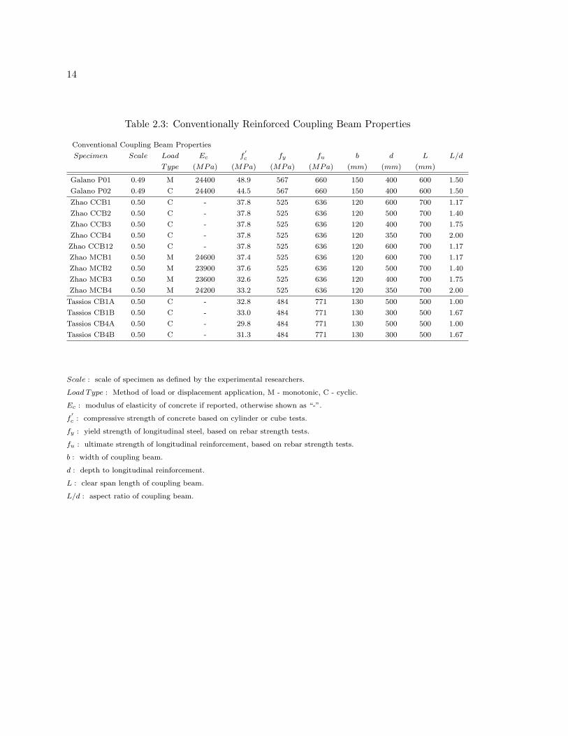
Data from the experimental tests of coupling beams include in this study were compiled
and evaluated to provide improved understanding of coupling beam performance. The tests
are separated into conventionally and diagonally reinforced coupling beam lots. The geom-
etry and material properties for each test specimen are summarized in Tables 2.3 and 2.5,
reinforcement details in Tables 2.4 and 2.6, and experimental results in Tables 2.7, 2.8,
and 2.9.
An evaluation of the impact of design parameters on the coupling beam performance
is discussed in Chapter 3. A reduced set of the twenty-two tests was used to evaluate the
finite element modeling capabilities of VecTor2; this is discussed in Chapter 4.
14
Table 2.3: Conventionally Reinforced Coupling Beam Properties
Conventional Coupling Beam Properties
Specimen Scale Load Ec f′c fy fu b d L L/d
Type (MPa) (MPa) (MPa) (MPa) (mm) (mm) (mm)
Galano P01 0.49 M 24400 48.9 567 660 150 400 600 1.50
Galano P02 0.49 C 24400 44.5 567 660 150 400 600 1.50
Zhao CCB1 0.50 C - 37.8 525 636 120 600 700 1.17
Zhao CCB2 0.50 C - 37.8 525 636 120 500 700 1.40
Zhao CCB3 0.50 C - 37.8 525 636 120 400 700 1.75
Zhao CCB4 0.50 C - 37.8 525 636 120 350 700 2.00
Zhao CCB12 0.50 C - 37.8 525 636 120 600 700 1.17
Zhao MCB1 0.50 M 24600 37.4 525 636 120 600 700 1.17
Zhao MCB2 0.50 M 23900 37.6 525 636 120 500 700 1.40
Zhao MCB3 0.50 M 23600 32.6 525 636 120 400 700 1.75
Zhao MCB4 0.50 M 24200 33.2 525 636 120 350 700 2.00
Tassios CB1A 0.50 C - 32.8 484 771 130 500 500 1.00
Tassios CB1B 0.50 C - 33.0 484 771 130 300 500 1.67
Tassios CB4A 0.50 C - 29.8 484 771 130 500 500 1.00
Tassios CB4B 0.50 C - 31.3 484 771 130 300 500 1.67
Scale : scale of specimen as defined by the experimental researchers.
Load Type : Method of load or displacement application, M - monotonic, C - cyclic.
Ec : modulus of elasticity of concrete if reported, otherwise shown as “-”.
f′c : compressive strength of concrete based on cylinder or cube tests.
fy : yield strength of longitudinal steel, based on rebar strength tests.
fu : ultimate strength of longitudinal reinforcement, based on rebar strength tests.
b : width of coupling beam.
d : depth to longitudinal reinforcement.
L : clear span length of coupling beam.
L/d : aspect ratio of coupling beam.

15
Table 2.4: Conventionally Reinforced Coupling Beam Reinforcement
Longitudinal Reinforcement Stirrups
Specimen #Long db Long As ρl #Side db Side db vert Av s ρv
Bars (mm) (mm2) Bars (mm) (mm) (mm2) (mm)
Galano P01 4 10 314.2 0.52% 2 6 6 56.5 80 0.84%
Galano P02 4 10 314.2 0.52% 2 6 6 56.5 80 0.84%
Zhao CCB1 3 12 334.8 0.49% 4 8 8 96.2 75 1.07%
Zhao CCB2 2, 1 12, 8 277.2 0.49% 4 8 8 96.2 75 1.07%
Zhao CCB3 2, 1 12, 8 277.2 0.50% 2 8 8 96.2 75 1.07%
Zhao CCB4 1, 2 12, 8 219.6 0.56% 2 8 8 96.2 75 1.07%
Zhao CCB12 3 12 335.0 0.49% 4 8 8 96.2 50 1.60%
Zhao MCB1 3 12 335.0 0.49% 4 8 8 96.2 75 1.07%
Zhao MCB2 2, 1 12, 8 277.2 0.49% 4 8 8 96.2 75 1.07%
Zhao MCB3 2 12 223.2 0.50% 2 8 8 96.2 75 1.07%
Zhao MCB4 1, 2 12, 8 219.2 0.56% 2 8 8 96.2 75 1.07%
Tassios CB1A 2 12 226.2 0.35% 4 6 8 100.5 75 1.03%
Tassios CB1B 2 12 226.2 0.58% 4 6 8 100.5 75 1.03%
Tassios CB4A 3 6 226.0 0.35% 4 20 8 100.5 75 1.03%
Tassios CB4B 3 6 226.0 0.58% 3 18 8 100.5 75 1.03%
#Long Bars : number of longitudinal reinforcement bars per side (top or bottom).
db Long : diameter of longitudinal reinforcement.
As : total area of longitudinal reinforcement.
ρl : longitudinal reinforcement ration, defined as Ast/db.
# Side : number of side or skin reinforcing bars.
db Side : diameter of side reinforcement.
db vert : diameter of vertical reinforcement or stirrups.
Av : area of stirrups.
s : spacing of stirrups.
ρv : vertical reinforcement ratio, defined as Av/sb.

16
Table 2.5: Diagonally Reinforced Coupling Beam Properties
Specimen Scale Load Ec f′c fy fu b d L L/d
Type (MPa) (MPa) (MPa) (MPa) (mm) (mm) (mm)
Galano P05 0.49 M 24400 39.9 567 660 150 400 600 1.50
Galano P07 0.49 C 24400 54.0 567 660 150 400 600 1.50
Galano P10 0.49 M 24400 46.8 567 660 150 400 600 1.50
Galano P12 0.49 C 24400 41.6 567 660 150 400 600 1.50
Zhao CCB11 0.50 C - 37.8 525 636 120 600 700 1.17
Tassios CB2A 0.50 C - 28.5 504 771 130 500 500 1.00
Tassios CB2B 0.50 C - 26.3 504 771 130 300 500 1.67
Scale : scale of specimen as defined by the experimental researchers.
Load Type : Method of load or displacement application, M - monotonic, C - cyclic.
Ec : modulus of elasticity of concrete if reported, otherwise shown as “-”.
f′c : compressive strength of concrete based on cylinder or cube tests.
fy : yield strength of longitudinal steel, based on rebar strength tests.
fu : ultimate strength of longitudinal reinforcement, based on rebar strength tests.
b : width of coupling beam.
d : depth to longitudinal reinforcement.
L : clear span length of coupling beam.
L/d : aspect ratio of coupling beam.

17
Table 2.6: Diagonally Reinforced Coupling Beam Reinforcement
Longitudinal Reinforcement Stirrups
Specimen #Long dbLong As ρl #Side dbSide dbvert Av s ρv
Bars (mm) (mm2) Bars (mm) (mm) (mm2) (mm)
Galano P05 2 6 85.0 0.14% 2 6 6 56.5 100 0.38%
Galano P07 2 6 85.0 0.14% 2 6 6 56.5 100 0.38%
Galano P10 2 6 85.0 0.14% 2 6 6 56.5 133 0.28%
Galano P12 2 6 85.0 0.14% 2 6 6 56.5 133 0.28%
Zhao CCB11 2 8 108.0 0.15% 4 8 8 92.6 140 0.55%
Tassios CB2A 3 6 84.8 0.13% 2 6 6 56.5 120 0.36%
Tassios CB2B 3 6 84.8 0.22% 2 6 6 56.5 120 0.36%
Table 2.6: (continued)
Diagonal Bars
Specimen No. dbdiag Ad ρd dbties sties
Bar/Diag (mm) (mm2) (mm) (mm)
Galano P05 4 10 314.2 0.52% None -
Galano P07 4 10 314.2 0.52% None -
Galano P10 4 10 314.2 0.52% 6 80
Galano P12 4 10 314.2 0.52% 6 80
Zhao CCB11 6 8 301.6 0.45% 6 60
Tassios CB2A 4 10 314.2 0.48% 6 50
Tassios CB2B 4 10 314.2 0.81% 6 50
#Long Bars : number of longitudinal reinforcement bars per side (top or bottom).
db Long : diameter of longitudinal reinforcement.
As : total area of longitudinal reinforcement.
ρl : longitudinal reinforcement ration, defined as Ast/db.
# Side Bars : number of side or skin reinforcing bars.
db Side : diameter of side reinforcement.
db vert : diameter of vertical reinforcement or stirrups.
Av : area of stirrups.
s : spacing of stirrups.
ρv : vertical reinforcement ratio, defined as Av/sb.
No Bar/Diag : number of diagonal reinforcement bars in each direction.
db diag : diameter of diagonal reinforcement.
Ad : total area of diagonal reinforcement.
ρd : diagonal reinforcement ratio, defined as Ad/db.
dbties : diameter of ties around diagonal bar group.
sties : spacing of ties around diagonal bar group.

18
Table 2.7: Coupling Beam Performance
Shear Strength Stiffness
Vy Vu V0.85Vu V1.5 V6.0 Ky Ku
Specimen (KN) (KN) (KN) (KN) (KN) (KN/mm) (KN/mm)
Conventional Longitudinal Reinforcement
Galano P01 223.9 223.9 190.3 225.0 150 44.3 9.3
Galano P02 210 230 195.5 225.0 120 41.2 13.7
Zhao CCB1 260 327 278.0 260.0 260 26.0 16.4
Zhao CCB2 190 227 193.0 220.0 - 31.7 18.9
Zhao CCB3 135 165 140.3 165.0 - 27.0 16.5
Zhao CCB4 110 123 104.6 123.0 75 18.3 10.3
Zhao CCB12 240 317 269.5 290.0 - 34.3 22.6
Zhao MCB1 262 344 292.4 265.0 344 25.0 7.6
Zhao MCB2 198 260 221.0 240.0 260 33.2 5.5
Zhao MCB3 126 159 135.2 150.0 159 31.5 3.8
Zhao MCB4 100 140 119.0 125.0 135 24.0 2.5
Tassios CB1A 179 212 180.2 180.0 - 22.9 12.5
Tassios CB1B 100 124 105.4 110.0 - 15.6 9.5
Tassios CB4A 282 282 239.7 - - 26.9 25.6
Tassios CB4B 162 162 137.7 - - 15.0 -
Average 185.2 219.7 186.8 198.3 187.9 27.8 12.5
Mean 190.0 223.9 190.3 220.0 154.5 26.9 11.4
Std. Dev. 61.5 74.2 63.1 59.8 90.4 8.5 6.9
Diagonal Reinforcement
Galano P05 220 239.3 203.4 230.0 220 43.5 7.4
Galano P07 215 240 204.0 230.0 140 42.6 16.0
Galano P10 220 241.1 204.9 230.0 210 47.3 7.4
Galano P12 210 245 208.3 240.0 - 45.2 18.6
Zhao CCB11 290 346 294.1 280.0 - 30.5 18.2
Tassios CB2A 214 283 240.6 215.0 - 28.9 -
Tassios CB2B 115 170 144.5 110.0 - 13.5 6.8
Average 212.0 252.1 214.2 219.3 190.0 35.9 12.4
Mean 215.0 241.1 204.9 230.0 210.0 42.6 11.7
Std. Dev. 51.1 53.2 45.2 52.3 43.6 12.2 5.8
Vy : yield strength of coupling beam as specified by researcher.
Vu : ultimate strength of coupling beam as specified by researcher.
V0.85Vu : 85% of Vu.
V1.5 : shear strength at 1.5% drift of coupling beam.
V6.0 : shear strength at 6.0% drift of coupling beam.
Ky : stiffness of coupling beam at the yield point, defined as Vy/δy .
Ku : stiffness of coupling beam at the ultimate strength point, defined as Vu/δu.

19
Table 2.8: Coupling Beam Capacity
Capacity
Mn Vp VnACI SSD
Specimen (KN − mm) (KN) (KN)
Conventional Longitudinal Reinforcement
Galano P01 60996 203.3 316.4 5.8
Galano P02 60996 203.3 313.6 6.1
Zhao CCB1 90283 258.0 425.5 7.0
Zhao CCB2 62292 178.0 354.6 5.8
Zhao CCB3 49833 142.4 283.7 5.8
Zhao CCB4 34544 98.7 248.2 4.6
Zhao CCB12 90336 258.1 603.9 7.0
Zhao MCB1 90336 258.1 425.2 7.0
Zhao MCB2 62292 178.0 354.4 5.8
Zhao MCB3 40126 114.6 280.6 5.0
Zhao MCB4 34481 98.5 245.8 4.9
Tassios CB1A 46861 187.4 343.5 6.0
Tassios CB1B 28117 112.5 206.2 6.0
Tassios CB4A 46820 187.3 340.9 6.3
Tassios CB4B 28092 112.4 205.3 6.2
Average 55094 172.7 329.9 5.9
Mean 49833 178.0 316.4 6.0
Std. Dev. 21692 57.8 101.5 0.7
Diagonal Reinforcement
Galano P05 59708 199.0 195.5 6.3
Galano P07 59708 199.0 195.5 5.4
Galano P10 59708 199.0 195.5 5.8
Galano P12 59708 199.0 195.5 6.1
Zhao CCB11 72646 207.6 203.9 5.6
Tassios CB2A 56380 225.5 221.6 7.8
Tassios CB2B 41022 164.1 161.2 9.8
Average 58411 199.0 195.5 6.7
Mean 59708 199.0 195.5 6.1
Std. Dev. 9272 18.2 17.9 1.6
Mn : moment strength of coupling beam calculated per ACI 318-05.
Vp : shear demand, calculated as 2Mp/L.
VnACI : shear strength of coupling beam calculated per ACI 318-05.
SSD shear stress demand, calculated as Vp/Ag
√(f
′c )

20
Table 2.9: Coupling Beam Drift, Displacement & Ductility
Drift Displacement Ductility
∆y ∆u ∆0.85Vu δy δu δ0.85u δ1.5 δ6.0 µu µ0.85u
Specimen (mm) (mm) (mm) (mm) (mm)
Conventional Longitudinal Reinforcement
Galano P01 0.84% 4.00% 5.09% 5.1 24.0 30.5 4.7 18.8 4.8 6.0
Galano P02 0.85% 2.80% 4.60% 5.1 16.8 27.6 4.7 18.8 3.3 5.4
Zhao CCB1 1.43% 2.86% 5.71% 10.0 20.0 40.0 5.0 20.1 2.0 4.0
Zhao CCB2 0.86% 1.71% 4.29% 6.0 12.0 30.0 4.2 16.6 2.0 5.0
Zhao CCB3 0.71% 1.43% 3.57% 5.0 10.0 25.0 4.2 16.6 2.0 5.0
Zhao CCB4 0.86% 1.71% 5.14% 6.0 12.0 36.0 3.3 13.2 2.0 6.0
Zhao CCB12 1.00% 2.00% 4.29% 7.0 14.0 30.0 5.0 20.1 2.0 4.3
Zhao MCB1 1.50% 6.43% 8.57% 10.5 45.0 60.0 5.0 20.1 4.3 5.7
Zhao MCB2 0.85% 6.71% 9.86% 6.0 47.0 69.0 4.2 16.6 7.9 11.6
Zhao MCB3 0.57% 6.00% 7.00% 4.0 42.0 49.0 3.3 13.4 10.5 12.3
Zhao MCB4 0.59% 8.14% 10.00% 4.2 57.0 70.0 3.3 13.2 13.7 16.8
Tassios CB1A 1.56% 3.40% 4.84% 7.8 17.0 24.2 3.4 13.6 2.2 3.1
Tassios CB1B 1.28% 2.60% 3.71% 6.4 13.0 18.6 3.4 13.6 2.0 2.9
Tassios CB4A 2.10% 2.20% 9.66% 10.5 11.0 48.3 3.4 13.6 1.0 4.6
Tassios CB4B 2.16% - 5.83% 10.8 - 29.2 3.4 13.6 - 2.7
Average 1.14% 3.71% 6.14% 7.0 24.3 39.2 4.0 16.1 4.3 6.4
Mean 0.86% 2.83% 5.14% 6.0 16.9 30.5 4.2 16.6 2.1 5.0
Std. Dev. 0.51% 2.20% 2.29% 2.4 16.1 16.5 0.7 2.9 3.8 4.0
Diagonal Reinforcement
Galano P05 0.84% 5.40% 6.54% 5.1 32.4 39.2 1.3 5.1 6.4 7.8
Galano P07 0.84% 2.50% 5.20% 5.1 15.0 31.2 1.3 5.1 3.0 6.2
Galano P10 0.78% 5.40% 6.20% 4.7 32.4 37.2 1.3 5.1 7.0 8.0
Galano P12 0.78% 2.20% 3.90% 4.7 13.2 23.4 1.3 5.1 2.8 5.0
Zhao CCB11 1.36% 2.71% 5.43% 9.5 19.0 38.0 1.6 6.5 2.0 4.0
Tassios CB2A 1.48% - 8.29% 7.4 - 41.4 1.3 5.1 - 5.6
Tassios CB2B 1.70% 5.00% 8.84% 8.5 25.0 44.2 1.3 5.1 2.9 5.2
Average 1.11% 3.87% 6.34% 6.4 22.8 36.4 1.3 5.3 4.0 6.0
Mean 0.84% 3.86% 6.20% 5.1 22.0 38.0 1.3 5.1 3.0 5.6
Std. Dev. 0.39% 1.55% 1.74% 2.0 8.4 7.0 0.1 0.5 2.1 1.5
δy : displacement at yield taken from load-displacment plots.
δu : displacement at ultimate shear force take from load displacement plots.
δ0.85Vu : displacement when shear force had dropped to 85% of Vu.
δ1.5 : displacement at 1.5% coupling beam drift.
δ6.0 : displacement at 6.0% coupling beam drift.
∆y : coupling beam drift at yield, δy/L.
∆u : coupling bean drift at ultimate shear force, δu/L.
µu : ultimate displacement ductility, δu/δy .
µ0.85Vu : displacement ductility when shear force had dropped to 85% of Vu, δ0.85Vu/δy .

21
2.4 Previous Analyses
2.4.1 Oyen
Oyen (2006) investigated the nonlinear modeling of planar shear walls and compared the
results from three types of analysis; lumped plasticity analysis using OpenSEES, section
analysis using Response-2000, and nonlinear continuum analysis using VecTor2. His inves-
tigations support the following conclusions:
• Accurate prediction of the peak strength requires the modeling of effects of shear.
• Accurate simulation of the displacement response requires the modeling of shear de-
formation.
• Inclusion of a bar-slip model can improve the simulation of the displacement response.
2.4.2 Brown
Brown (2006) assembled a large database of previous experimental tests of planar walls. He
developed fragility functions to define the probability that a specific method of repair will be
required to restore a damaged planar wall to pre-earthquake condition. He also developed
effective stiffness versus drift relationships for the experimental tests. The effective stiffness
data was then used to calibrate models predicting the decay of flexural stiffness. Refer to
Peter Brown’s thesis for information about effective stiffness of shear walls.
2.4.3 Zhao et. al.
Zhao et al. (2004) investigated the behavior of deep coupling beams using a nonlinear finite
element method they recently developed. Since the method has been presented in detail
elsewhere, only a summary is presented herein.
The concrete and steel are modeled together by a four-noded isoparametric quadrilateral
plane stress element with two extra non-conforming bending modes intended to remove
22
shear locking. The constitutive model of the element consists of two parts, one for the
concrete and one for the steel. The concrete takes into consideration the biaxial behavior
of the material, assuming isotropic behavior before cracking and orthotropic after cracking.
Tension softening and compression softening are allowed for in the stress-strain relationships.
A smeared crack model is utilized. The steel model assumes that the reinforcing bars are
perfectly bonded to the concrete and uniformly smeared throughout the element. A tri-
linear stress-strain behavior is assumed. Stress transfer across cracks due to bond and
dowel action is accounted for. This method is very similar to the Modified Compression
Field Theory, however it is not referred to as such by the author.
The above method was used to analyze four monotonically loaded, conventionally re-
inforced coupling beams. The analytical models include the test specimen and the entire
loading frame. The author was able to predict the ultimate strength with an average over-
estimation of only 6.2%. The analytical models were able to reach deflections that corre-
sponded very well with the measured deflection at maximum load. However, the appearance
of the load deflection curves does not agree very well with the experimental measured curves.
The analytical specimens have a much higher stiffness prior to yield and reach the maxi-
mum load very early in the loading, whereas the experimental results gradually approach
the maximum load near the end of the displacement history.
The author noted two main reasons for the discrepancies in the load-deflection curves
of the analytical vs. experimental specimens.
1. The increased initial stiffness is due to the perfect bond model between the reinforcing
bars and the concrete. In the experimental specimens flexural cracks gradually opened
up and bond-slip of the main reinforcing bars occurred. The opening of the flexural
cracks and slip of the reinforcing bars made a significant contribution to the lateral
deflections of the coupling beam specimens, and thus reduced the initial stiffness.
2. In a real structure, tension strains are concentrated at the cracks and the concrete
between cracks continues to contribute to the resistance of the structure through

23
tension stiffening. Use of the smeared crack model does not allow for proper modeling
of the strain localization and tension stiffening that occurs in-between adjacent cracks
formed in a real structure. This discrepancy caused the analytical models to loose
strength rapidly after reaching the peak load and caused an underestimation of the
post-yield effective stiffness.

24
Chapter 3
COUPLING BEAM PERFORMANCE AND DAMAGE PATTERNS
The behavior modes of coupling beams can vary widely from one configuration to an-
other. The twenty two experimental coupling beams were compared to examine the influence
of coupling beam parameters and performance measures on the observed behavior mode. In
order to do this the behavior modes had to be defined and then assigned to each specimen.
The following sections present the definition of the behavior modes, photographs of the
specimens at failure, and plots comparing the behavior mode to various parameters.
3.1 Behavior Mode Definition
The coupling beams exhibited a wide variety of behavior and failure modes. In order to
identify the failure mode of each specimen a clearly defined set of behavior criteria had to
be developed. FEMA 306 provides a “Component Damage Classification Guide” for various
reinforced concrete elements, however the specified behavior modes for coupling beams do
not cover all of those observed. Six behavior modes were identified, the CB1 behavior modes
are primarily seen in conventionally reinforced coupling beams while the CB2 modes are
primarily seen in diagonally reinforced coupling beams. The behavior modes adapted from
FEMA 306 and the additional ones defined are as follows:
CB1A Ductile Flexure: Spalling or vertical cracking occurs at toe regions in plastic
hinge zone, typically limited to cover concrete. No buckled or fractured reinforce-
ment.
CB1B Preemptive Diagonal Tension: For low levels of damage, appearance is similar
to CB1A. At heavy damage levels behavior is characterized by wide diagonal cracks,

25
18
′′ to 38
′′, extending from one corner of the beam to the other. Shear cracking is
typically concentrated in a single crack.
CB1C Flexure/Diagonal Tension: For low levels of damage appearance is similar to
CB1A. At heavy damage levels diagonal shear cracks become more prominent. Shear
crack widths may exceed 18
′′ but do not exceed 38
′′. Higher width cracking is concen-
trated to one or more cracks.
CB1D Flexure/Sliding Shear: Development of a major vertical flexural crack along the
entire beam depth, with some degradation of concrete along the crack, indicating that
sliding has occurred. Possible small lateral offset at crack.
CB2G Diagonal Compression: Spalling of concrete at the center of the coupling beam
where the two diagonal bar groups intersect. Flexural cracking occurs and ends of
beam with wide diagonal shear cracks parallel to the diagonal reinforcement. Bucking
of diagonal reinforcement may occur at the center of the coupling beam, within area
of spalling.
CB2F Flexure Compression: Spalling and flexural cracking occurs at the toe regions in
the plastic hinge zone. Diagonal shear cracks occur throughout the beam, typically fol-
lowing the direction of the diagonal reinforcement. Bucking of diagonal reinforcement
may occur at the ends of the coupling beam.
3.2 Experimental Behavior Modes
The coupling beam behavior modes were determined based on photographs of the speci-
mens found in the published reports and observations of the behavior by the experimental
researchers. Table 3.1 shows the behavior modes for all the experimental coupling beams
along with the parameters studied in section 3.3. Photographs of the coupling beams at
failure are presented and grouped by behavior mode.

26
Table 3.1: Coupling Beam Behavior Modes
Specimen AR Behavior SSD Bond ∆u ρv ρd µu
Mode Demand
Conventional Longitudinal Reinforcement
Galano P01 1.5 CB1B 5.8 60.0 4.00% 0.52% 0.84% 4.8
Galano P02 1.5 CB1A 6.1 60.0 2.80% 0.52% 0.84% 3.3
Tassios CB1A 1.0 CB1C 6.0 41.7 3.40% 0.35% 1.03% 2.2
Tassios CB1B 1.7 CB1B 6.0 41.7 2.60% 0.58% 1.03% 2.0
Tassios CB4A 1.0 CB1C 6.3 83.3 2.20% 0.35% 1.03% 1.0
Tassios CB4B 1.7 CB1C 6.2 83.3 - 0.58% 1.03% -
Zhao CCB1 1.2 CB1C 7.0 58.3 2.86% 0.49% 1.07% 2.0
Zhao CCB2 1.4 CB1B 5.8 58.3 1.71% 0.49% 1.07% 2.0
Zhao CCB3 1.8 CB1D 5.8 58.3 1.43% 0.50% 1.07% 2.0
Zhao CCB4 2.0 CB1C 4.6 58.3 1.71% 0.56% 1.07% 2.0
Zhao CCB12 1.2 CB1D 7.0 58.3 2.00% 0.49% 1.60% 2.0
Zhao MCB1 1.2 CB1B 7.0 58.3 6.43% 0.49% 1.07% 4.3
Zhao MCB2 1.4 CB1C 5.8 58.3 6.71% 0.49% 1.07% 7.9
Zhao MCB3 1.8 CB1A 5.0 58.3 6.00% 0.50% 1.07% 10.5
Zhao MCB4 2.0 CB1A 4.9 58.3 8.14% 0.56% 1.07% 13.7
Average 1.4 - 6.0 68.2 3.45% 0.49% 1.12% 3.7
Median 1.4 - 6.0 58.3 2.20% 0.49% 1.07% 2.0
Std. Dev 0.3 - 0.8 10.5 2.24% 0.06% 0.17% 3.3
Diagonal Reinforcement
Galano P05 1.5 - 6.3 72.1 5.40% 0.39% 0.52% 6.4
Galano P07 1.5 CB2G 5.4 72.1 2.50% 0.39% 0.52% 3.0
Galano P10 1.5 - 5.8 72.1 5.40% 0.31% 0.52% 7.0
Galano P12 1.5 CB2G 6.1 72.1 2.20% 0.31% 0.52% 2.8
Tassios CB2A 1.0 CB2F 7.8 70.7 - 0.36% 0.48% -
Tassios CB2B 1.7 CB2F 9.8 58.3 5.00% 0.36% 0.81% 2.9
Zhao CCB11 1.2 CB2G 5.6 115.2 2.71% 0.57% 0.45% 2.0
Average 1.4 - 6.7 68.2 3.87% 0.38% 0.55% 4.0
Median 1.5 - 6.1 72.1 3.86% 0.36% 0.52% 3.0
Std. Dev 0.2 - 1.6 18.0 1.55% 0.09% 0.12% 2.1

27
Zhao MCB4 Zhao MCB3
Galano P16
Figure 3.1: CB1A - Ductile Flexure

28
Galano P01
Zhao MCB1
Figure 3.2: CB1B - Preemptive Diagonal Tension

29
Tassios CB1B
Zhao CCB1 Zhao CCB2
Zhao CCB4 Zhao MCB2
Figure 3.3: CB1C - Flexure/Diagonal Tension

30
Zhao CCB3
Zhao CCB12
Figure 3.4: CB1D - Flexure/Sliding Shear
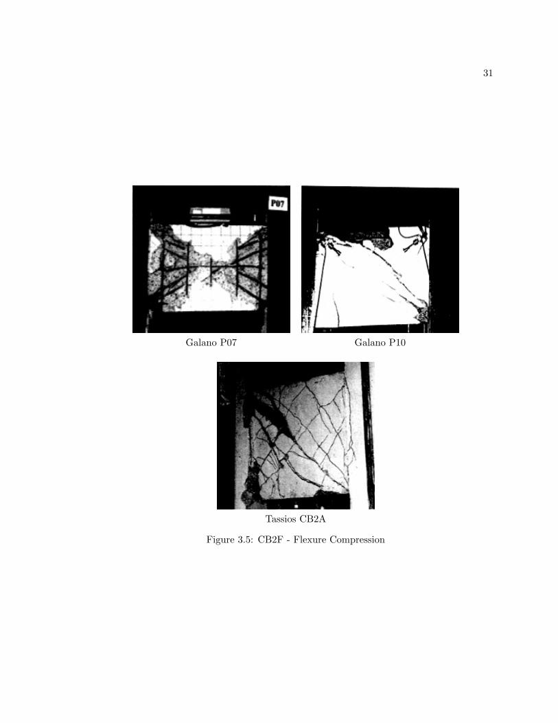
31
Galano P07 Galano P10
Tassios CB2A
Figure 3.5: CB2F - Flexure Compression
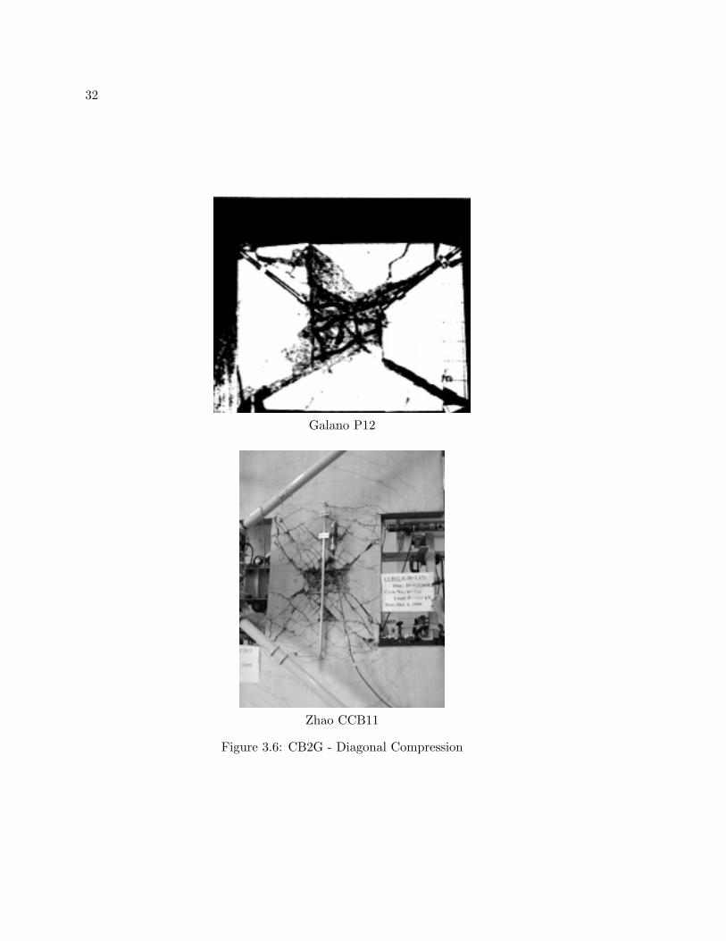
32
Galano P12
Zhao CCB11
Figure 3.6: CB2G - Diagonal Compression

33
3.3 Comparison Plots
For the conventionally reinforced coupling beams the aspect ratio, ρl, ρv, SSD, and bond
demand were plotted against µu and ∆u. For the diagonally reinforced coupling beams the
aspect ratio, ρd, ρv, SSD, and bond demand were plotted against µu and ∆u. For each
comparison a plot was created with the data sorted by the behavior mode.
There were no discernible trends found between the behavior mode and the various
parameters studied, this could be due to the wide variations in the coupling beam configu-
rations that are included in this data set.

34
0.5
0.7
0.9
1.1
1.3
1.5
1.7
1.9
2.1
0.0 5.0 10.0 15.0Ultimate Ductility, µu
Asp
ect R
atio
CB1ACB1BCB1CCB1D
Figure 3.7: Conv. Reinf. Coupling Beams - Displacement Ductility vs. Aspect Ratio
0.0%
1.0%
2.0%
3.0%
4.0%
5.0%
6.0%
7.0%
8.0%
9.0%
0.0 5.0 10.0 15.0Ultimate Ductility, µu
Ulti
mat
e D
rift, Δ
u
CB1ACB1BCB1CCB1D
Figure 3.8: Conv. Reinf. Coupling Beams - Displacement Ductility vs. Ultimate Displace-ment

35
0.3%
0.3%
0.4%
0.4%
0.5%
0.5%
0.6%
0.6%
0.0 5.0 10.0 15.0Ultimate Ductility, µu
ρl L
ong.
Rei
nf. R
atio
CB1ACB1BCB1CCB1D
Figure 3.9: Conv. Reinf. Coupling Beams - Displacement Ductility vs. LongitudinalReinforcement Ratio
0.7%
0.8%
0.9%
1.0%
1.1%
1.2%
1.3%
1.4%
1.5%
1.6%
1.7%
0.0 5.0 10.0 15.0Ultimate Ductility, µ
ρv V
ert.
Rei
nf. R
atio
CB1ACB1BCB1CCB1D
Figure 3.10: Conv. Reinf. Coupling Beams - Displacement Ductility vs. Vertical Reinforce-ment Ratio

36
4
5
5
6
6
7
7
8
0.0 2.0 4.0 6.0 8.0 10.0 12.0 14.0 16.0Ultimate Ductility, µu
She
ar S
tress
Dem
and
CB1ACB1BCB1CCB1D
Figure 3.11: Conv. Reinf. Coupling Beams - Displacement Ductility vs. Shear StressDemand
30
40
50
60
70
80
90
0.0 2.0 4.0 6.0 8.0 10.0 12.0 14.0 16.0
Ultimate Ductility, µu
Bon
d D
eman
d
CB1ACB1BCB1CCB1D
Figure 3.12: Conv. Reinf. Coupling Beams - Displacement Ductility vs. Bond StressDemand

37
0.3%
0.3%
0.4%
0.4%
0.5%
0.5%
0.6%
0.6%
0.0% 2.0% 4.0% 6.0% 8.0% 10.0%Ultimate Drift, Δu
ρl L
ong.
Rei
nf. R
atio
CB1ACB1BCB1CCB1D
Figure 3.13: Conv. Reinf. Coupling Beams - Ultimate Displacement vs. LongitudinalReinforcement Ratio
0.8%
0.9%
1.0%
1.1%
1.2%
1.3%
1.4%
1.5%
1.6%
1.7%
0.0% 2.0% 4.0% 6.0% 8.0% 10.0%Ultimate Drift, Δu
ρv V
ert.
Rei
nf. R
atio
CB1ACB1BCB1CCB1D
Figure 3.14: Conv. Reinf. Coupling Beams - Ultimate Displacement vs. Vertical Reinforce-ment Ratio

38
1.0
1.1
1.2
1.3
1.4
1.5
1.6
1.7
0.0 2.0 4.0 6.0 8.0Ultimate Ductility, µu
Asp
ect R
atio
CB2GCB2FN/ACBR
Figure 3.15: Diag. Reinf. Coupling Beams - Displacement Ductility vs. Aspect Ratio
1.0%
2.0%
3.0%
4.0%
5.0%
6.0%
0.0 2.0 4.0 6.0 8.0Ultimate Ductility, µu
Ulti
mat
e D
rift, Δ
u
CB2GCB2FN/A
Figure 3.16: Diag. Reinf. Coupling Beams - Displacement Ductility vs. Ultimate Displace-ment

39
0.3%
0.4%
0.5%
0.6%
0.7%
0.8%
0.9%
1.0%
0.0 2.0 4.0 6.0 8.0Ultimate Ductility, µu
ρd D
iag.
Rei
nf. R
atio
CB2GCB2FN/ACBR
Figure 3.17: Diag. Reinf. Coupling Beams - Displacement Ductility vs. Diagonal Rein-forcement Ratio
0.3%
0.3%
0.4%
0.4%
0.5%
0.5%
0.6%
0.6%
0.0 2.0 4.0 6.0 8.0Ultimate Ductility, µu
ρv V
ert.
Rei
nf. R
atio
CB2GCB2FN/A
Figure 3.18: Diag. Reinf. Coupling Beams - Displacement Ductility vs. Vertical Reinforce-ment Ratio

40
4
5
6
7
8
9
10
11
0.0 1.0 2.0 3.0 4.0 5.0 6.0 7.0 8.0
Ultimate Ductility, µu
She
ar S
tress
Dem
and
CB2GCB2FN/A
Figure 3.19: Diag. Reinf. Coupling Beams - Displacement Ductility vs. Shear StressDemand
40
50
60
70
80
90
100
110
120
0.0 1.0 2.0 3.0 4.0 5.0 6.0 7.0 8.0
Ultimate Ductility, µu
Bon
d D
eman
d
CB2GCB2FN/A
Figure 3.20: Diag. Reinf. Coupling Beams - Displacement Ductility vs. Bond StressDemand
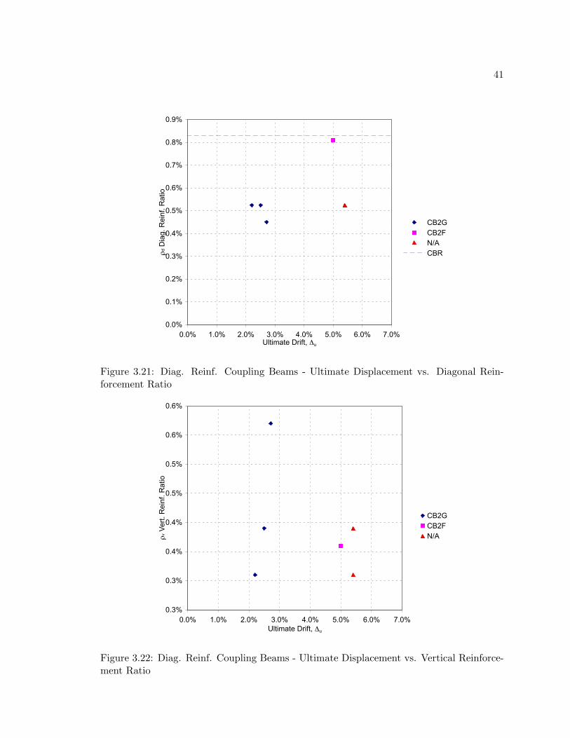
41
0.0%
0.1%
0.2%
0.3%
0.4%
0.5%
0.6%
0.7%
0.8%
0.9%
0.0% 1.0% 2.0% 3.0% 4.0% 5.0% 6.0% 7.0%Ultimate Drift, Δu
ρd D
iag.
Rei
nf. R
atio
CB2GCB2FN/ACBR
Figure 3.21: Diag. Reinf. Coupling Beams - Ultimate Displacement vs. Diagonal Rein-forcement Ratio
0.3%
0.3%
0.4%
0.4%
0.5%
0.5%
0.6%
0.6%
0.0% 1.0% 2.0% 3.0% 4.0% 5.0% 6.0% 7.0%Ultimate Drift, Δu
ρv V
ert.
Rei
nf. R
atio
CB2GCB2FN/A
Figure 3.22: Diag. Reinf. Coupling Beams - Ultimate Displacement vs. Vertical Reinforce-ment Ratio

42
Chapter 4
NONLINEAR FINITE ELEMENT ANALYSIS OFCOUPLING BEAM EXPERIMENTS
In this chapter, nonlinear finite element analysis of the experimental coupling beam data
set introduced in Chapter 2 is presented, the results are compared to the observed response,
and the capabilities of the analysis software are discussed. Analyses were completed using
VecTor2 c© (Vecchio and Wong 2006), a nonlinear finite element analysis program that
utilizes two-dimensional continuum elements. The following sections describe the modeling
parameters, constitutive models and modeling decisions for all of the simulations and present
in detail the analytical results of three representative coupling beams. Full results for all of
the coupling beams are presented in Appendix A.
4.1 VecTor2
VecTor2 is a computer program for the analysis of two-dimensional reinforced concrete
structures. This program has been in ongoing development at the University of Toronto
since 1990. The development of the program has been combined with experimental tests to
support the abilities of VecTor2 to predict the load-deformation response of reinforced con-
crete structures. The program is based on the Modified Compression Field Theory (Vecchio
and Collins 1986) and the Disturbed Stress Field Model (Vecchio 2000), both are analytical
models for predicting the response of reinforced concrete elements subjected to in-plane
normal and shear stresses. Cracked concrete is modeled as an orthotropic material with
smeared cracks that are allowed to rotate. The program uses an incremental total load and
iterative secant stiffness algorithm to solve for the nonlinear solution.
VecTor2 incorporates a number of constitutive models for second-order effects including
compression softening, tension stiffening, tension softening, and tension splitting. It allows

43
the modeling of concrete confinement and expansion, crack shear slip deformations, dowel
action of reinforcement, bar buckling, bond slip, hysteretic behavior, and loading history.
Finite element models are intended to include a fine mesh of elements that should be
sufficient to capture the reinforcement patterns, local deformations and crack patterns.
It’s element library includes a four-node plane stress rectangular element, a four-node plane
stress quadrilateral element, and a three-node constant strain triangle for modeling concrete
with smeared reinforcement; a two-node truss-bar element for modeling discrete reinforce-
ment; and a two-node link and four-node contact element for modeling bond-slip.
VecTor2 provides a graphical preprocessor program, FormWorks c© , to facilitate model
building and visual confirmation of the data. It provides tools for automatic mesh generation
and model optimization to minimize computational demands. The companion software
program Augustus c© provides a graphical environment for post-processing the analytical
results of VecTor2.
4.2 Modeling Decisions
Specification of a model in VecTor2 requires the definition of material properties, constitu-
tive models, element mesh, reinforcement, boundary conditions, and a load or displacement
history. Each of these items are presented and discussed in the following sections.
4.2.1 Material Properties
Reported material properties, where available, were used for all specimens. Details of the
material properties are presented in Tables 2.3 and 2.5 from Chapter 2.
4.2.2 Constitutive Models
VecTor2 provides a large number of constitutive models for concrete and reinforcement.
With the exception of the following, concrete compression pre and post-peak response, and
concrete compression softening response, the default material properties were used.

44
The default constitutive model for the compressive pre-peak response is the Hognestad
(Parabola) model and the default for compression post-peak response is the Modified Park-
Kent model. Preliminary parameter studies found that the default concrete models caused
a rapid loss of strength after the peak compressive strain was reached. This rapid loss of
strength lead to a decrease in the displacement ductility of the specimen and an undesirable
load-displacement response. The combination of the Popovics Normal Strength Concrete
pre-peak response and the Popovics/Mander post-peak response provided a slower strength
loss and thus allowed for larger displacement ductilities to be reached. The Popovics (NSC)
and Popovics/Mander concrete constitutive models were used in all of the coupling beam
simulations.
Compression softening occurs in cracked concrete and is the reduction of compressive
strength and stiffness, in relation to the uniaxial compressive strength, due to the effects of
transverse cracking and tensile straining. In VecTor2, compression softening is effected by
the softening parameter βd, which is calculated by the compression softening model. The
models are based on statistical analysis of the stress-strain states of selected panel elements
tested at the University of Tornono (Vecchio and Collins, 1992). The compression softening
models are divided into two types; strength-and-strain softening and strength-only softening
models.
Strength-and-strain softening models use the βd factor to reduce both the compressive
strength, f′c, and the corresponding strain, ε0, to determine the peak compressive strength
and peak compressive strain. Strength-only softening models use the βd factor to reduce
only the compressive strength, f′c, to determine the peak compressive stress, while the cor-
responding strain, ε0, remains unmodified. The default constitutive model for compression
softening is the Vecchio 1992-A (e1/e2-Form), a strength-and-strain softening model. Pre-
liminary parameter studies suggest that the Vecchio 1992-B (e1/e0-Form), a strength-only
compression softening model, provided a better approximation of the strength approxima-
tion at large displacements than the default model. The Vecchio 1992-B (e1/e0-Form)
compression softening model was used in all of the coupling beam simulations.

45
Table 4.1: Constitutive Models used in Coupling Beam Simulations
Constitutive Behavior Model
Compression Base Curve Popovics (NSC)
Compression Post-Peak Popovics / Mander
Compression Softening Vecchio 1992-B (e1/e0-Form)
Tension Stiffening Modified Bentz 2003
Tension Softening Bilinear
Tension Splitting Not Considered
Confinement Strength Kupfer / Richart Model
Concrete Dilation Variable - Kupfer
Cracking Criterion Mohr-Coulomb (stress)
Crack Slip Check Vecchio-Collins 1986
Crack Width Check Agg/5 Max Crack Width
Slip Distortions Vecchio-Lai
Concrete Hysteresis Nonlinear w/ Plastic Offsets
Steel Hysteresis Elastic-Plastic w/ Hardening
Rebar Dowel Action Tassios (Crack Slip)
The default models were used for tension stiffening, tension softening, confinement, lat-
eral expansion, crack slip, crack width, concrete hysteresis response, dowel action, and
reinforcement hysteresis response. A complete list of the constitutive models used in shown
in Table 4.1, and the analysis parameters used are shown in Table 4.2. The default consti-
tutive models available in VecTor2 are documented in detail in the user manual (Vecchio
and Wong 2006), and can be found online at (www.civ.utoronto.ca/vector).
4.2.3 Element Mesh
The FormWorks program provides automatic mesh generation capabilities based on user
input parameters of element type, maximum element size, and maximum aspect ratio.
These parameters can be changed for different regions to allow for varying levels of mesh

46
Table 4.2: Analysis Parameters used in Coupling Beam Simulations
Analysis Parameter Model
Convergence Criteria Displacements - Weighted
Strain History Previous Loading Considered
Strain Rate Effects Not Considered
Structural Damping Not Considered
Geometric Nonlinearity Considered
Crack Allocation Process Uniform
refinement and element type within the model.
Element Type
The element type can be of three types, rectangular, quadrilateral, and/or triangular. Vec-
Tor2 allows for the mixing of all three element types within in model. For the conventionally
reinforced coupling beams the mesh was composed solely of rectangular elements. This was
possible because of the completely orthogonal geometry of the model. For the diagonally
reinforced coupling beams the mesh was a combination of all three element types. The
details of the mesh layout are handled by the FormWorks program and its automatic mesh
generation capabilities.
Element Size
A preliminary parameter study was completed to determine the effect of element size on the
performance of a coupling beam model. A conventionally reinforced coupling beam, taken
from the experimental data-set, was modeled with three different levels of mesh refinement
and compared to the reported load-displacement curve, the results are shown in Figure 4.1.
The d/7.5 mesh size is too coarse, causing a false stiffening of the coupling beam and
resulting in larger yield and ultimate capacities than the reported values. The d/15 mesh
size does not cause as much of an over-prediction of the yield force and provides a close

47
0 10 20 30 40 50 60 700
20
40
60
80
100
120
140
160
180
200
She
ar (
KN
)
Displacement (mm)
Effect of Mesh Refinement
Experimentald/7.5 meshd/15 meshd/25 mesh
Figure 4.1: Effect of Mesh Refinement
agreement with the reported load-displacement curve through the initial portion of the
load-displacement curve. The d/24 mesh size showed a small improvement over the d/15
mesh in regard to matching the experimental yield strength, however it also began to loose
strength at an earlier displacement level.
These results suggest that the quality of the finite element simulation shows a mesh size
dependency. Given the incremental gross over-prediction of the d/7.5 mesh the unfavorable
early strength loss of the d/24 mesh, a maximum mesh size of d/15 for the coupling beams
was chosen. This ratio was used as a guideline for all subsequent coupling beam models.
Aspect Ratio
VecTor2 allows the maximum aspect ratio for elements to be specified. During the automatic
meshing process this limit will be followed and the element size adjusted to the largest

48
possible dimension that will meet the maximum aspect ratio. For all the coupling beam
models the default aspect ratio of 1.5 was used.
4.2.4 Types of Reinforcement
VecTor2 allows for the reinforcement to be modeled in two different manners. Reinforcement
can be modeled as a distributed reinforcement using a specified ratio, commonly referred to
as smeared reinforcement, or as discrete truss-bar elements. For all of the coupling beams,
both methods of modeling the reinforcement were used and two versions of each model were
carried through the entire study.
• Smeared Reinforcement: For these models, all of the reinforcement in the coupling
beam and in the loading blocks was modeled using smeared reinforcement elements.
Reinforcement ratios, taken from the experimental data-set (Tables 2.4 & 2.6), were
specified for each of the three primary directions; longitudinal, vertical, and out of
plane.
• Truss-Bar Reinforcement: For these models the primary reinforcement was modeled
with truss-bar elements and all other reinforcement was modeled using smeared rein-
forcement elements. For conventionally reinforced coupling beams the primary rein-
forcement is defined as the top and bottom longitudinal bars. For diagonally reinforced
coupling beams, the primary reinforcement is defined as the diagonal reinforcing bars.
The truss-bar elements were extended into the loading blocks a minimum of the bar
development length. The reinforcement ratios for the vertical and out-of-plane rein-
forcement remain the same as the smeared reinforcement models. The longitudinal
reinforcement ratio was taken as the area of the nominal longitudinal bars over the
cross section area of the coupling beam.

49
4.2.5 Boundary Conditions
There were three types experimental test set-ups found in in the experimental coupling
beam data-set. The different test set-ups are presented and described in detail in Chap-
ter 2. Despite the differences in the experimental test configurations, they all seek to impose
the same set of forces and displacements on the coupling beam specimen; imposing a con-
stant shear force and shear deformation on the coupling beam without restraining axial
deformations.
A single set of boundary conditions were used for all of the coupling beam models. To
represent the loading conditions in the laboratory, the top and bottom edges of the left
loading block were restrained against motion in the vertical direction, and the right edge
of he right loading block was restrained against motion in the horizontal direction. These
boundary conditions allowed for the ends of the coupling beam loading blocks to remain
parallel without causing any axial restraint on the specimen.
4.2.6 Loading Parameters
A vertical displacement was applied to all of the nodes along the right edge of the right load
block. For monotonically loaded specimens the displacement was applied incrementally up
to the reported maximum displacement or until the model became numerically unstable.
For cyclically loaded specimens the reported displacement history from the experimental
test was replicated. When the experimental loading history was not available, the specimens
were cycled three times at the yield displacement and then cycled three times at increasing
multiples of the yield displacement, δy, 2δy,4δy, and then pushed monotonically until failure.
4.3 Description of Evaluation Method
The quality of the predicted results are compared to the reported experimental response to
determine the quality of the VecTor2 simulations. The performance parameters used in this
study include:

50
l/d: coupling beam aspect ratio.
δy: is the displacement in the simulation at the point when the reported yield shear strength
was reached.
δu: is the displacement in the simulation at the predicted maximum shear force was reached.
∆y: is the drift in the coupling beam simulation at the point when the reported yield shear
strength was reached.
∆u: is the drift in the coupling beam simulation at the predicted maximum shear force.
∆0.85Vu: is the drift in the coupling beam at the point where 85% of the maximum predicted
shear, Vu, was reached.
DCR : is the demand capacity ratio defines as the maximum shear force, Vu, divided by
the design strength, Vn.
Ky : is the secant stiffness at the reported point of first yield.
Ku: is the secant stiffness at the reported ultimate shear force.
K1.5%: is the secant stiffness corresponding to 1.5% drift in the coupling beam.
K6.0%: is the secant stiffness corresponding to 6.0% drift in the coupling beam.
Vy: is the shear in the coupling beam when first yielding is reported by the experimental
researcher.
Vu: is the maximum shear observed in the coupling beam.
V1.5%: is the shear in the coupling beam at 1.5% drift, for the 10-Story reference wall this
corresponds to 0.5% story drift and is the expected point of first yield.
51
V6.0%: is the shear in the coupling beam at 6.0% drift, for the 10-story reference wall this
corresponds to 2.0% story drift and is the maximum design level drift.
SSD: shear stress demand, defined as Vp/Agf′c
where
Vp = 2Mn/l,
Mn = flexural strength of coupling beam based on the longitudinal or diagonal rein-
forcement depending on the configuration,
l = coupling beam clear span length,
Ag = coupling beam cross section area, and
f′c = compressive strength of concrete.
These simulation results and comparisons to the observed data are shown in Table 4.3
through 4.5.

52
Table 4.3: Experimental Coupling Beam Strength Predictions
Specimen Vy Vy/Vye Vu Vu/Vue V1.5% V6.0%
GalanoP01 DT 200.6 0.90 239.9 1.07 238.0 27.9
GalanoP02 DT 196.6 0.94 234.4 1.00 230.5 0.0
GalanoP05 DT 166.6 0.76 221.7 0.93 221.7 -5.8
GalanoP07 T 236.9 1.10 244.2 1.02 244.2 0.0
GalanoP10 DT 226.3 1.03 239.0 0.99 238.0 10.8
GalanoP12 DT 223.0 1.06 234.6 0.96 234.6 0.0
TassiosCB1A DT 203.2 1.14 214.3 1.01 214.2 0.0
TassiosCB1B DT 149.9 1.50 149.9 1.21 141.5 0.0
TassiosCB2A DT 202.0 0.94 210.1 0.74 179.9 0.0
TassiosCB2B DT 135.9 1.18 158.7 0.93 156.0 0.0
ZhaoCCB11 T 324.6 1.12 348.9 1.01 298.3 0.0
ZhaoCCB2 DT 220.7 1.16 229.1 1.01 198.6 0.0
ZhaoCCB4 DT 94.8 0.86 129.4 1.05 118.0 0.0
ZhaoMCB1 DT 291.7 1.11 295.0 0.86 266.7 0.8
ZhaoMCB2 DT 226.7 1.14 244.8 0.94 221.7 0.8
ZhaoMCB3 DT 132.9 1.05 161.3 1.01 151.1 0.7
ZhaoMCB4 DT 88.7 0.89 126.1 0.90 116.8 0.0
Average 195.4 1.05 216.6 0.98 204.1 5.9
Median 202.0 1.06 229.1 1.00 221.7 0.8
Std.Dev. 62.8 0.17 58.0 0.10 52.3 12.0
Max 324.6 1.50 348.9 1.21 298.3 27.9
Min 88.7 0.76 126.1 0.74 116.8 -5.8
Strength (V) in KN
∗ 0 values indicate data not available

53
Table 4.4: Experimental Coupling Beam Stiffness Predictions
Specimen Ky Ky/Kye Ku Ku/Kue K1.5 K1.5/K1.5e K6 K6/K6e
GalanoP01 DT 36.6 0.83 26.7 2.9 28.1 1.12 0.8 0.18
GalanoP02 DT 32.9 0.80 22.4 1.8 25.7 1.03 0.0 0.00
GalanoP05 DT 41.7 0.97 26.1 3.5 26.1 1.02 -0.2 -0.03
GalanoP07 T 31.1 0.74 26.7 1.7 26.7 1.04 0.0 0.00
GalanoP10 DT 34.9 0.75 29.9 4.0 28.0 1.10 0.3 0.05
GalanoP12 DT 31.7 0.71 27.8 1.5 27.8 1.04 0.0 0.00
TassiosCB1A DT 41.2 1.79 31.1 2.5 27.2 1.13 0.0 0.00
TassiosCB1B DT 25.1 1.60 25.1 2.6 20.3 1.38 0.0 0.00
TassiosCB2A DT 41.3 1.43 30.8 1.6 23.5 0.82 0.0 0.00
TassiosCB2B DT 34.1 2.52 6.6 1.0 22.4 1.52 0.0 0.00
ZhaoCCB11 T 59.5 1.95 39.0 2.1 30.0 1.12 0.0 0.00
ZhaoCCB2 DT 40.2 1.27 38.3 2.0 18.9 0.90 0.0 0.00
ZhaoCCB4 DT 35.1 1.92 21.6 2.1 10.9 0.93 0.0 0.00
ZhaoMCB1 DT 41.8 1.68 39.5 5.2 26.7 1.06 0.0 0.00
ZhaoMCB2 DT 41.3 1.25 35.1 6.3 22.2 0.97 0.0 0.00
ZhaoMCB3 DT 33.3 1.06 17.0 4.5 15.1 1.06 0.0 0.00
ZhaoMCB4 DT 35.5 1.49 15.8 6.4 11.7 0.98 0.0 0.00
Average 37.5 1.34 27.0 3.0 23.0 1.07 0.1 0.01
Median 35.5 1.27 26.7 2.5 25.7 1.04 0.0 0.00
Std.Dev. 7.4 0.52 8.8 1.7 5.8 0.17 0.2 0.05
Max 59.5 2.52 39.5 6.4 30.0 1.52 0.8 0.18
Min 25.1 0.71 6.6 1.0 10.9 0.82 -0.2 -0.03
Stiffness (K) in KN-mm
∗ 0 values indicate data not available

54
Table 4.5: Experimental Coupling Beam Displacement and Drift Predictions
Specimen δy δy/δye δu δu/δue ∆y ∆y/∆ye ∆u ∆u/∆ue ∆0.85Vu
GalanoP01 DT 5.5 1.07 9.0 0.37 0.91% 1.07 1.50% 0.38 5.37%
GalanoP02 DT 6.0 1.17 10.5 0.62 1.00% 1.18 1.75% 0.63 3.47%
GalanoP05 DT 4.0 0.78 8.5 0.26 0.67% 0.79 1.41% 0.26 2.13%
GalanoP07 T 7.6 1.49 9.2 0.61 1.27% 1.49 1.52% 0.61 2.95%
GalanoP10 DT 6.5 1.38 8.0 0.25 1.08% 1.38 1.33% 0.25 2.30%
GalanoP12 DT 7.0 1.50 8.5 0.64 1.17% 1.49 1.41% 0.64 2.36%
TassiosCB1A DT 4.9 0.63 6.9 0.41 0.99% 0.63 1.38% 0.41 2.56%
TassiosCB1B DT 6.0 0.93 6.0 0.46 1.20% 0.94 1.20% 0.46 -
TassiosCB2A DT 4.9 0.66 6.8 0.45 0.98% 0.66 1.36% 0.45 3.50%
TassiosCB2B DT 4.0 0.47 24.0 0.92 0.80% 0.47 4.80% 0.92 -
ZhaoCCB11 T 5.5 0.57 8.9 0.47 0.78% 0.57 1.28% 0.47 2.56%
ZhaoCCB2 DT 5.5 0.92 6.0 0.50 0.78% 0.91 0.86% 0.50 2.81%
ZhaoCCB4 DT 2.7 0.45 6.0 0.50 0.39% 0.46 0.86% 0.50 2.60%
ZhaoMCB1 DT 7.0 0.66 7.5 0.17 1.00% 0.67 1.07% 0.17 2.81%
ZhaoMCB2 DT 5.5 0.92 7.0 0.15 0.78% 0.91 1.00% 0.15 3.35%
ZhaoMCB3 DT 4.0 1.00 9.5 0.23 0.57% 1.00 1.36% 0.23 3.21%
ZhaoMCB4 DT 2.5 0.60 8.0 0.14 0.36% 0.60 1.14% 0.14 4.00%
Average 5.2 0.89 8.8 0.42 0.87% 0.90 1.48% 0.42 3.07%
Median 5.5 0.92 8.0 0.45 0.91% 0.91 1.36% 0.45 2.81%
Std.Dev. 1.5 0.34 4.1 0.21 0.26% 0.34 0.89% 0.21 0.82%
Max 7.6 1.50 24.0 0.92 1.27% 1.49 4.80% 0.92 5.37%
Min 2.5 0.45 6.0 0.14 0.36% 0.46 0.86% 0.14 2.13%
Displacement (δ) in mm

55
4.4 Reduced Data Set for Illustration of VecTor2 Capabilities
Selected coupling beams were chosen to illustrate the capabilities of VecTor2. The selected
coupling beams represent the two methods of loading, monotonic vs. cyclic, and the two
reinforcement patterns, conventional vs. diagonal reinforcement.
The three test specimens are:
• Galano P01 - monotonically loaded with conventional reinforcement,
• Galano P02 - cyclically loaded with conventional reinforcement (same reinforcement
as Galano P01), and
• Tassios CB2B - cyclically loaded with diagonal reinforcement.
4.5 Description of Results
4.5.1 Galano P01
Figures 4.2 and 4.3 show the simulated load-displacement response and the experimental
response history. Figures 4.4 - 4.6 show crack patterns at reported yield strength, predicted
ultimate strength and 80% of the predicted ultimate strength. Initial yielding of the primary
longitudinal reinforcement is predicted at a drift of 0.42%, corresponding to a 142.9-KN
applied load. The reported drift at yield was 0.85%, with a 223.9-KN applied load. However,
the reported yield strength and drift corresponds to the point where the stiffness changes
abruptly and the load-displacement response begins to level out, whereas the initial yield
in the VecTor2 simulation is taken as the first point where the yield stress was reached in
the longitudinal reinforcment. Comparing the predicted strength at the reported yield drift
results in a much closer comparison; a predicted strength of 200.6-KN, an under-prediction
of 10% (Figure 4.2).
The model continues to gain strength up to the maximum value of 239.9-KN at a drift
of 1.50%. The maximum strength is over-predicted by 10%, however the drift at maximum

56
strength is greatly under-predicted with ratio of predicted-to-observed of 0.38. The dis-
placement and cracking at the predicted maximum strength are shown in Figure 4.5. This
figure shows that wide cracks are beginning to form in the web elements at the left end of
the beam. The web elements have a smaller horizontal reinforcement ratio than the two
elements at the top and bottom of the beam representing the longitudinal reinforcement,
and can be expected to provide less resistance to tensile cracking. The majority of the
elements in the coupling beam have diagonally oriented crack directions following a diago-
nal compression strut from one end of the beam to the other, indicating that the beam is
primarily behaving in a shear mode. At the predicted maximum strength, all of the primary
longitudinal steel has yielded and entered into the strain hardening region.
As displacement is increased beyond the point of maximum strength, the predicted
strength drops abruptly due to crushing in the extreme compression elements. The com-
pressive stress is redistributed around the crushed elements and the strength then levels
out to a value near the experimental peak strength. As the compressive elements crush the
vertical strain is increased and the shear reinforcement begins to yield near the ends of the
coupling beam.
The model begins to loose strength at 4.7% drift, which is very close to the initiation of
strength loss in the experiment. Wide flexural cracks have opened up at both ends of the
beam and continue through approximately half of the beam depth an then transition to shear
cracks in the compression zone. Skewed elements and diagonal cracking in the compression
zone indicate a concentration of shear stress and strain distortion. At this load step, yielding
of the shear reinforcement has occurred and is spread over the first four elements at each
end of the coupling beam, or 1/6 of the length. Rapid strength loss continues at drifts
greater than 4.7%. Figure 4.6 shows wide shear cracks concentrated at the left interface of
the coupling beam and the loading block in conjunction with significantly skewed elements,
indicating a large concentration of shear strain and stress at this location. The predicted
failure mode is similar to a sliding-shear failure, however the experimental specimen failed
due to fracture of the stirrups at one end of the beam and resulted in the opening of a single

57
large diagonal crack extending from one corner of the beam to the other, (Figure 4.7).
4.5.2 Galano P02
Figures 4.8 and 4.9 show the simulated load-displacement response and the experimental
response history. Figures 4.10 - 4.12 show crack patterns at reported yield strength, pre-
dicted ultimate strength and 80% of the predicted ultimate strength. Initial yielding of the
primary longitudinal reinforcement is predicted in the third displacement cycle at a drift of
0.42% and a shear force of 140.7-KN. The force at the experimental reported yield drift was
196.6-KN, compared to the reported yield force of 211-KN. The predicted ultimate force or
234-KN was the same as reported from the experiment, however it did occur at lower drift
level, 1.75% vs. 2.78%, only 63% of the reported value. In the negative displacement di-
rection, the peak strength was 208.4-KN, which is again very close to the reported strength
of 213-KN. The displacement and cracking at the predicted ultimate strength are shown in
Figure 4.11. At this load step, wide cracks are beginning to form in the web elements of the
coupling beam. Flexural cracks are still present in the extreme tensile zones at each end
of the coupling beam, but quickly transition into diagonal cracks toward the center of the
beam.
In the displacement cycle following the peak strength, the specimen was only able to
reach 200-KN in the positive direction, and 194.5-KN in the negative direction. The pre-
dicted shear strengths at yield, ultimate and the cycles following the ultimate strength are
very close to the reported values, all with an under-prediction of less than 10%.
The behavior of the simulation and the experiment began to diverge after the peak
strength was reached. The simulation began to loose strength at an earlier drift level and
at a faster rate. The simulation began to loose substantial strength (more than 20%) at
3.3% drift compared to approximately 5.0% in the experiment. Additionally, when the
strength loss in the simulation dropped all the way to zero, where the experiment retained
approximately 20% of the peak.
The strength loss of the simulation was due to a sliding-failure. All of the longitudi-

58
nal reinforcement had yielded and gone through strain hardening, at the load step where
strength loss occurred, the steel fractured and lost all of its load carrying capacity. The
failure in the longitudinal steel allowed the concrete to expand axially and undergo large
shear deformations without any additional force, and resulted in the sudden shear slip at
the ends of the coupling beam. Figure 4.12 shows the displaced shape and crack pattern at
80% of Vu, the concentration of shear deformation can be seen at both ends of the beam.
While VecTor2 was able to provide a good prediction of the strength and deformation
response, the failure mode was not correct. In the experiment the coupling beam experienced
heavy spalling over the middle half of the beam and into the corners, however the ends
remained relatively intact as seen in Figure 4.13.
4.5.3 Tasssios CB2B
Figures 4.14 and 4.15 show the simulated load-displacement response and the experimen-
tal response history. Figures 4.16 - 4.18 show crack patterns at reported yield strength,
predicted ultimate strength and the predicted maximum displacement.

59
0 10 20 30 40 50 600
50
100
150
200
250
300
She
ar (
KN
)
Displacement (mm)
Galano P01
ExperimentalVector − Smeared
Figure 4.2: VecTor2 Predicted Response of Galano P01
Figure 4.3: Experimental Response of Galano Specimens

60
Figure 4.4: Displaced Shape and Crack Pattern at Vy of Galano P01
Figure 4.5: Displaced Shape and Crack Pattern at Vu of Galano P01

61
Figure 4.6: Displaced Shape and Crack Pattern at 0.8Vu of Galano P01
Figure 4.7: Experimental Failure of Galano P01
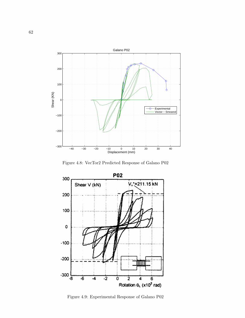
62
−40 −30 −20 −10 0 10 20 30 40−300
−200
−100
0
100
200
300S
hear
(K
N)
Displacement (mm)
Galano P02
ExperimentalVector − Smeared
Figure 4.8: VecTor2 Predicted Response of Galano P02
Figure 4.9: Experimental Response of Galano P02

63
Figure 4.10: Displaced Shape and Crack Pattern at Vy of Galano P02
Figure 4.11: Displaced Shape and Crack Pattern at Vu of Galano P02

64
Figure 4.12: Displaced Shape and Crack Pattern at 0.8Vu of Galano P02
Figure 4.13: Experimental Failure of Galano P02

65
−30 −20 −10 0 10 20 30−200
−150
−100
−50
0
50
100
150
200
She
ar (
KN
)
Displacement (mm)
Tassios CB2B
ExperimentalVector − Smeared
Figure 4.14: VecTor2 Predicted Response of Tassios CB2B
Figure 4.15: Experimental Response of Tassios CB2B

66
Figure 4.16: Displaced Shape and Crack Pattern at Vy of Tassios CB2B
Figure 4.17: Displaced Shape and Crack Pattern at Vu of Tassios CB2B

67
Figure 4.18: Displaced Shape and Crack Pattern at ∆max of Tassios CB2B
Figure 4.19: Experimental Failure of Tassios CB2B

68
4.6 Data Analysis and Trends
The results of the Experimental Coupling Beam simulations were plotted versus various
engineering demand parameters to investigate any patterns in the behavior. The model
results were first separated by the loading method, monotonic or cyclical. The following
results, Vy, Vu, δu, Ky, and Ku, were plotted against the aspect ratio, ρv, shear demand to
capacity ratio, and the shear stress demand. The strength and displacement results were
normalized against the experimental results.
No discernible trends were discovered in the studied response parameters. The plots
have been included for informational purposes.

69
1.3 1.4 1.5 1.6 1.7 1.8 1.9 20.85
0.9
0.95
1
1.05
1.1
1.15
1.2
Lb / d
Vy /
Vye
Monotonic Coupling BeamsYield Force vs Aspect Ratio
Diag Reinf. VctConv Reinf. Vct
Figure 4.20: Mono. Coupling Beams - Yield Strength vs. Aspect Ratio
0.2 0.3 0.4 0.5 0.6 0.7 0.8 0.9 1 1.1 1.20.85
0.9
0.95
1
1.05
1.1
1.15
1.2
ρv
Vy /
Vye
Monotonic Coupling BeamsYield Force vs Vertical Reinf. Ratio
Diag Reinf. VctConv Reinf. Vct
Figure 4.21: Mono. Coupling Beams - Yield Strength vs. Vertical Reinforcement Ratio
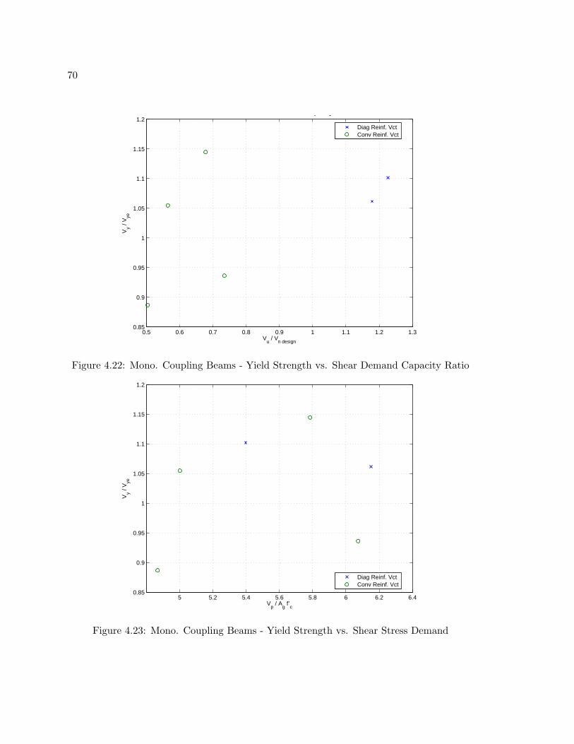
70
0.5 0.6 0.7 0.8 0.9 1 1.1 1.2 1.30.85
0.9
0.95
1
1.05
1.1
1.15
1.2
Vu / V
n design
Vy /
Vye
Monotonic Coupling BeamsYield Force vs Shear Demand Capacity Ratio
Diag Reinf. VctConv Reinf. Vct
Figure 4.22: Mono. Coupling Beams - Yield Strength vs. Shear Demand Capacity Ratio
5 5.2 5.4 5.6 5.8 6 6.2 6.40.85
0.9
0.95
1
1.05
1.1
1.15
1.2
Vp / A
g f’
c
Vy /
Vye
Monotonic Coupling BeamsYield Force vs Shear Stress Demand
Diag Reinf. VctConv Reinf. Vct
Figure 4.23: Mono. Coupling Beams - Yield Strength vs. Shear Stress Demand

71
1.3 1.4 1.5 1.6 1.7 1.8 1.9 20.9
0.92
0.94
0.96
0.98
1
1.02
Lb / d
Vu /
Vue
Monotonic Coupling BeamsUltimate Shear vs Aspect Ratio
Diag Reinf. VctConv Reinf. Vct
Figure 4.24: Mono. Coupling Beams - Ultimate Strength vs. Aspect Ratio
0.2 0.3 0.4 0.5 0.6 0.7 0.8 0.9 1 1.1 1.20.9
0.92
0.94
0.96
0.98
1
1.02
ρv
Vu /
Vue
Monotonic Coupling BeamsUltimate Shear vs Vertical Reinf. Ratio
Diag Reinf. VctConv Reinf. Vct
Figure 4.25: Mono. Coupling Beams - Ultimate Strength vs. Vertical Reinforcement Ratio

72
0.5 0.6 0.7 0.8 0.9 1 1.1 1.2 1.30.9
0.92
0.94
0.96
0.98
1
1.02
Vu / V
n design
Vu /
Vue
Monotonic Coupling BeamsUltimate Shear vs Shear Demand Capacity Ratio
Diag Reinf. VctConv Reinf. Vct
Figure 4.26: Mono. Coupling Beams - Ultimate Strength vs. Shear Demand Capacity Ratio
5 5.2 5.4 5.6 5.8 6 6.2 6.40.9
0.92
0.94
0.96
0.98
1
1.02
Vp / A
g f’
c
Vu /
Vue
Monotonic Coupling BeamsUltimate Shear vs Shear Stress Demand
Diag Reinf. VctConv Reinf. Vct
Figure 4.27: Mono. Coupling Beams - Ultimate Strength vs. Shear Stress Demand

73
1.3 1.4 1.5 1.6 1.7 1.8 1.9 20.1
0.2
0.3
0.4
0.5
0.6
0.7
0.8
Lb / d
δ u / δ ue
Monotonic Coupling BeamsUltimate Displacement vs Aspect Ratio
Diag Reinf. VctConv Reinf. Vct
Figure 4.28: Mono. Coupling Beams - Ultimate Displacement vs. Aspect Ratio
0.2 0.3 0.4 0.5 0.6 0.7 0.8 0.9 1 1.1 1.20.1
0.2
0.3
0.4
0.5
0.6
0.7
0.8
ρv
δ u / δ ue
Monotonic Coupling BeamsUltimate Displacement vs Vertical Reinf. Ratio
Diag Reinf. VctConv Reinf. Vct
Figure 4.29: Mono. Coupling Beams - Ultimate Displacement vs. Vertical ReinforcementRatio
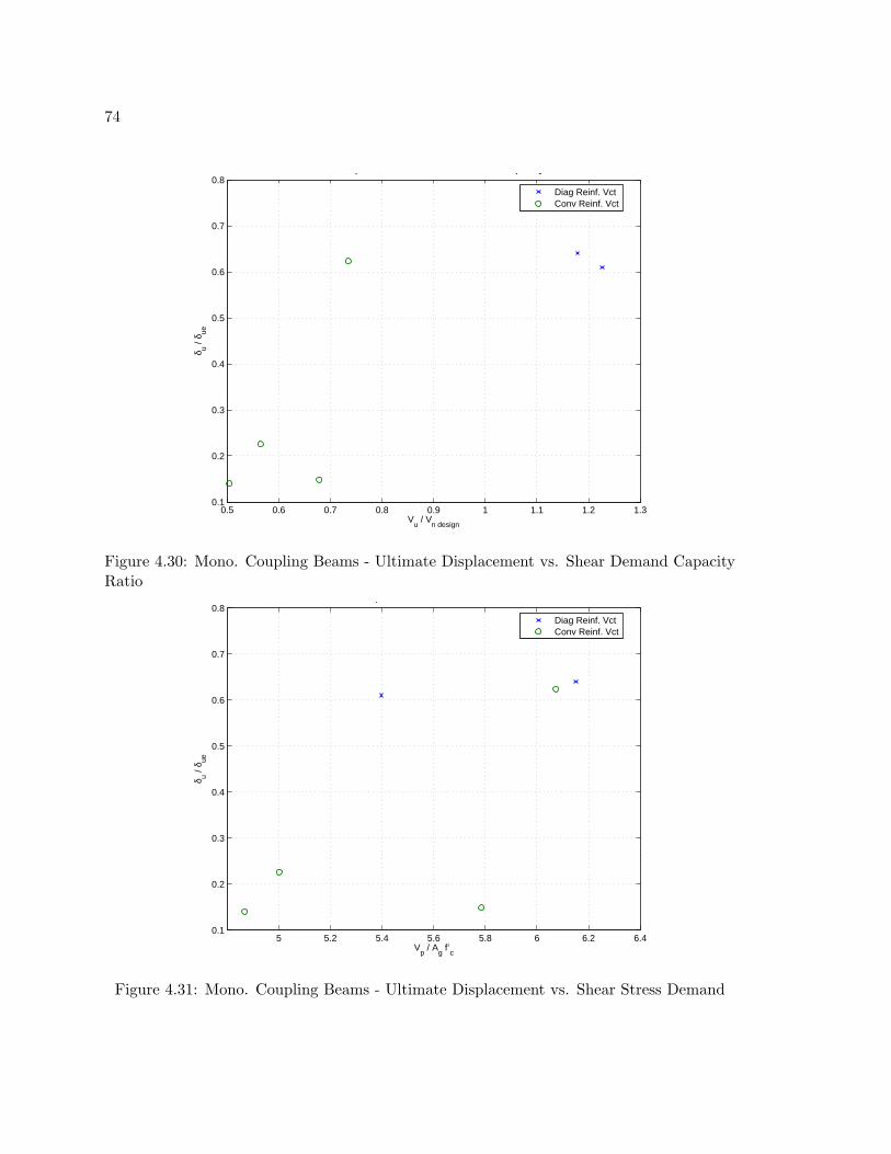
74
0.5 0.6 0.7 0.8 0.9 1 1.1 1.2 1.30.1
0.2
0.3
0.4
0.5
0.6
0.7
0.8
Vu / V
n design
δ u / δ ue
Monotonic Coupling BeamsUltimate Displacement vs Shear Demand Capacity Ratio
Diag Reinf. VctConv Reinf. Vct
Figure 4.30: Mono. Coupling Beams - Ultimate Displacement vs. Shear Demand CapacityRatio
5 5.2 5.4 5.6 5.8 6 6.2 6.40.1
0.2
0.3
0.4
0.5
0.6
0.7
0.8
Vp / A
g f’
c
δ u / δ ue
Monotonic Coupling BeamsUltimate Displacement vs Shear Stress Demand
Diag Reinf. VctConv Reinf. Vct
Figure 4.31: Mono. Coupling Beams - Ultimate Displacement vs. Shear Stress Demand

75
1.3 1.4 1.5 1.6 1.7 1.8 1.9 20.015
0.02
0.025
0.03
0.035
0.04
Lb / d
Ky/ K
elas
tic
Monotonic Coupling BeamsYield Stiffness vs Aspect Ratio
Diag Reinf. Exp.Conv Reinf. Exp.Diag Reinf. VctConv Reinf. Vct
Figure 4.32: Mono. Coupling Beams - Yield Stiffness vs. Aspect Ratio
0.2 0.3 0.4 0.5 0.6 0.7 0.8 0.9 1 1.1 1.20.015
0.02
0.025
0.03
0.035
0.04
ρv
Ky/ K
elas
tic
Monotonic Coupling BeamsYield Stiffness vs Vertical Reinf. Ratio
Diag Reinf. Exp.Conv Reinf. Exp.Diag Reinf. VctConv Reinf. Vct
Figure 4.33: Mono. Coupling Beams - Yield Stiffness vs. Vertical Reinforcement Ratio
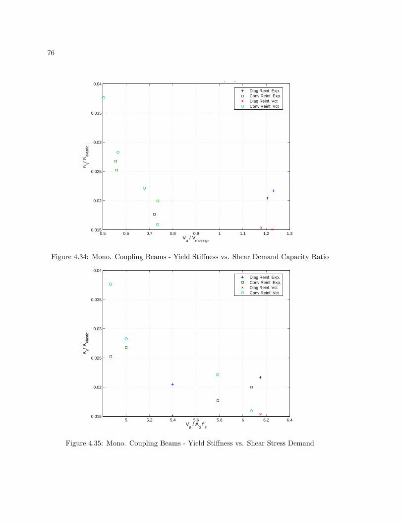
76
0.5 0.6 0.7 0.8 0.9 1 1.1 1.2 1.30.015
0.02
0.025
0.03
0.035
0.04
Vu / V
n design
Ky/ K
elas
tic
Monotonic Coupling BeamsYield Stiffness vs Shear Demand Capacity Ratio
Diag Reinf. Exp.Conv Reinf. Exp.Diag Reinf. VctConv Reinf. Vct
Figure 4.34: Mono. Coupling Beams - Yield Stiffness vs. Shear Demand Capacity Ratio
5 5.2 5.4 5.6 5.8 6 6.2 6.40.015
0.02
0.025
0.03
0.035
0.04
Vp / A
g f’
c
Ky/ K
elas
tic
Monotonic Coupling BeamsYield Stiffness vs Shear Stress Demand
Diag Reinf. Exp.Conv Reinf. Exp.Diag Reinf. VctConv Reinf. Vct
Figure 4.35: Mono. Coupling Beams - Yield Stiffness vs. Shear Stress Demand

77
1.3 1.4 1.5 1.6 1.7 1.8 1.9 20.002
0.004
0.006
0.008
0.01
0.012
0.014
0.016
0.018
0.02
Lb / d
Ku/ K
elas
tic
Monotonic Coupling BeamsUltimate Stiffness vs Aspect Ratio
Diag Reinf. Exp.Conv Reinf. Exp.Diag Reinf. VctConv Reinf. Vct
Figure 4.36: Mono. Coupling Beams - Ultimate Stiffness vs. Aspect Ratio
0.2 0.3 0.4 0.5 0.6 0.7 0.8 0.9 1 1.1 1.20.002
0.004
0.006
0.008
0.01
0.012
0.014
0.016
0.018
0.02
ρv
Ku/ K
elas
tic
Monotonic Coupling BeamsUltimate Stiffness vs Vertical Reinf. Ratio
Diag Reinf. Exp.Conv Reinf. Exp.Diag Reinf. VctConv Reinf. Vct
Figure 4.37: Mono. Coupling Beams - Ultimate Stiffness vs. Vertical Reinforcement Ratio
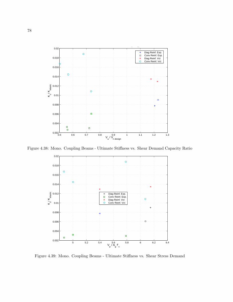
78
0.5 0.6 0.7 0.8 0.9 1 1.1 1.2 1.30.002
0.004
0.006
0.008
0.01
0.012
0.014
0.016
0.018
0.02
Vu / V
n design
Ku/ K
elas
tic
Monotonic Coupling BeamsUltimate Stiffness vs Shear Demand Capacity Ratio
Diag Reinf. Exp.Conv Reinf. Exp.Diag Reinf. VctConv Reinf. Vct
Figure 4.38: Mono. Coupling Beams - Ultimate Stiffness vs. Shear Demand Capacity Ratio
5 5.2 5.4 5.6 5.8 6 6.2 6.40.002
0.004
0.006
0.008
0.01
0.012
0.014
0.016
0.018
0.02
Vp / A
g f’
c
Ku/ K
elas
tic
Monotonic Coupling BeamsUltimate Stiffness vs Shear Stress Demand
Diag Reinf. Exp.Conv Reinf. Exp.Diag Reinf. VctConv Reinf. Vct
Figure 4.39: Mono. Coupling Beams - Ultimate Stiffness vs. Shear Stress Demand
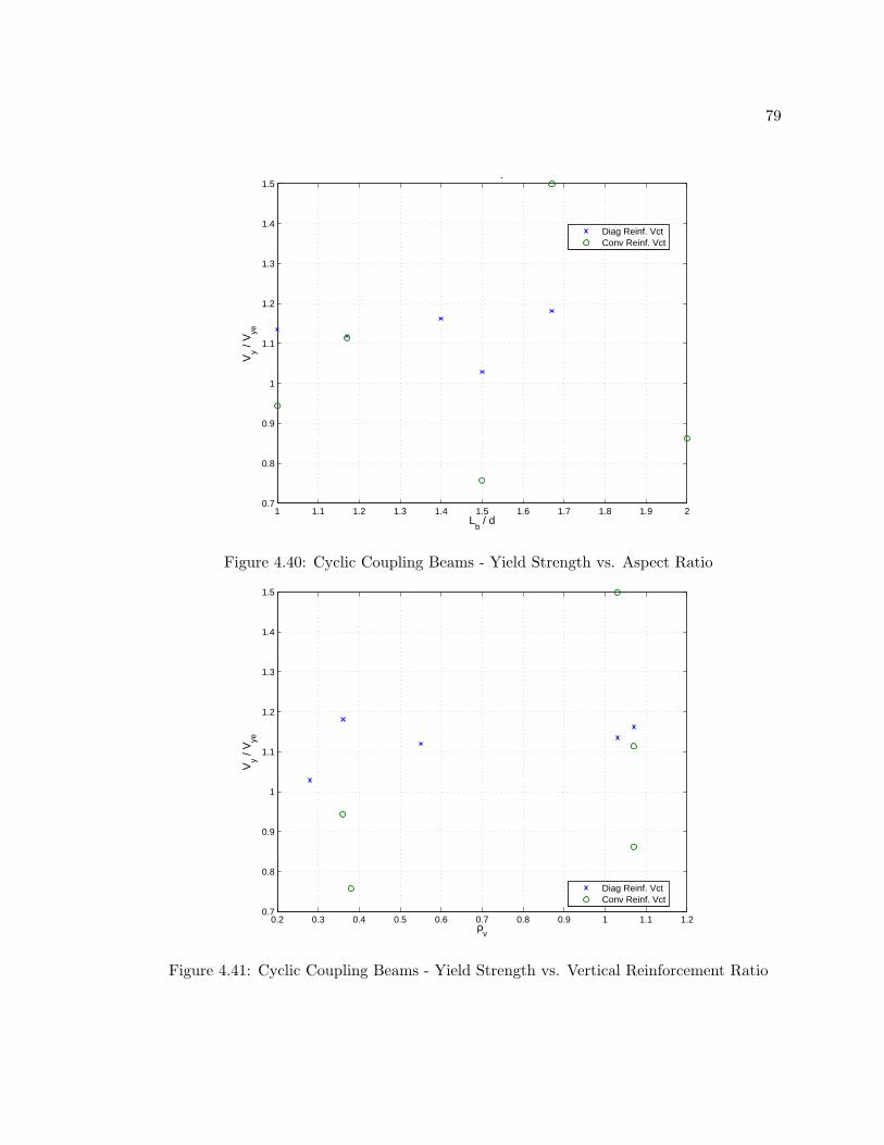
79
1 1.1 1.2 1.3 1.4 1.5 1.6 1.7 1.8 1.9 20.7
0.8
0.9
1
1.1
1.2
1.3
1.4
1.5
Lb / d
Vy /
Vye
Cyclic Coupling BeamsYield Force vs Aspect Ratio
Diag Reinf. VctConv Reinf. Vct
Figure 4.40: Cyclic Coupling Beams - Yield Strength vs. Aspect Ratio
0.2 0.3 0.4 0.5 0.6 0.7 0.8 0.9 1 1.1 1.20.7
0.8
0.9
1
1.1
1.2
1.3
1.4
1.5
ρv
Vy /
Vye
Cyclic Coupling BeamsYield Force vs Vertical Reinf. Ratio
Diag Reinf. VctConv Reinf. Vct
Figure 4.41: Cyclic Coupling Beams - Yield Strength vs. Vertical Reinforcement Ratio

80
0.4 0.6 0.8 1 1.2 1.4 1.6 1.80.7
0.8
0.9
1
1.1
1.2
1.3
1.4
1.5
Vu / V
n design
Vy /
Vye
Cyclic Coupling BeamsYield Force vs Shear Demand Capacity Ratio
Diag Reinf. VctConv Reinf. Vct
Figure 4.42: Cyclic Coupling Beams - Yield Strength vs. Shear Demand Capacity Ratio
4 5 6 7 8 9 100.7
0.8
0.9
1
1.1
1.2
1.3
1.4
1.5
Vp / A
g f’
c
Vy /
Vye
Cyclic Coupling BeamsYield Force vs Shear Stress Demand
Diag Reinf. VctConv Reinf. Vct
Figure 4.43: Cyclic Coupling Beams - Yield Strength vs. Shear Stress Demand

81
1 1.1 1.2 1.3 1.4 1.5 1.6 1.7 1.8 1.9 20.7
0.8
0.9
1
1.1
1.2
1.3
Lb / d
Vu /
Vue
Cyclic Coupling BeamsUltimate Shear vs Aspect Ratio
Diag Reinf. VctConv Reinf. Vct
Figure 4.44: Cyclic Coupling Beams - Ultimate Strength vs. Aspect Ratio
0.2 0.3 0.4 0.5 0.6 0.7 0.8 0.9 1 1.1 1.20.7
0.8
0.9
1
1.1
1.2
1.3
ρv
Vu /
Vue
Cyclic Coupling BeamsUltimate Shear vs Vertical Reinf. Ratio
Diag Reinf. VctConv Reinf. Vct
Figure 4.45: Cyclic Coupling Beams - Ultimate Strength vs. Vertical Reinforcement Ratio

82
0.4 0.6 0.8 1 1.2 1.4 1.6 1.80.7
0.8
0.9
1
1.1
1.2
1.3
Vu / V
n design
Vu /
Vue
Cyclic Coupling BeamsUltimate Shear vs Shear Demand Capacity Ratio
Diag Reinf. VctConv Reinf. Vct
Figure 4.46: Cyclic Coupling Beams - Ultimate Strength vs. Shear Demand Capacity Ratio
4 5 6 7 8 9 100.7
0.8
0.9
1
1.1
1.2
1.3
Vp / A
g f’
c
Vu /
Vue
Cyclic Coupling BeamsUltimate Shear vs Shear Stress Demand
Diag Reinf. VctConv Reinf. Vct
Figure 4.47: Cyclic Coupling Beams - Ultimate Strength vs. Shear Stress Demand

83
1 1.1 1.2 1.3 1.4 1.5 1.6 1.7 1.8 1.9 20.1
0.2
0.3
0.4
0.5
0.6
0.7
0.8
0.9
1
Lb / d
δ u / δ ue
Cyclic Coupling BeamsUltimate Displacement vs Aspect Ratio
Diag Reinf. VctConv Reinf. Vct
Figure 4.48: Cyclic Coupling Beams - Ultimate Displacement vs. Aspect Ratio
0.2 0.3 0.4 0.5 0.6 0.7 0.8 0.9 1 1.1 1.20.1
0.2
0.3
0.4
0.5
0.6
0.7
0.8
0.9
1
ρv
δ u / δ ue
Cyclic Coupling BeamsUltimate Displacement vs Vertical Reinf. Ratio
Diag Reinf. VctConv Reinf. Vct
Figure 4.49: Cyclic Coupling Beams - Ultimate Displacement vs. Vertical ReinforcementRatio

84
0.4 0.6 0.8 1 1.2 1.4 1.6 1.80.1
0.2
0.3
0.4
0.5
0.6
0.7
0.8
0.9
1
Vu / V
n design
δ u / δ ue
Cyclic Coupling BeamsUltimate Displacement vs Shear Demand Capacity Ratio
Diag Reinf. VctConv Reinf. Vct
Figure 4.50: Cyclic Coupling Beams - Ultimate Displacement vs. Shear Demand CapacityRatio
4 5 6 7 8 9 100.1
0.2
0.3
0.4
0.5
0.6
0.7
0.8
0.9
1
Vp / A
g f’
c
δ u / δ ue
Cyclic Coupling BeamsUltimate Displacement vs Shear Stress Demand
Diag Reinf. VctConv Reinf. Vct
Figure 4.51: Cyclic Coupling Beams - Ultimate Displacement vs. Shear Stress Demand

85
1 1.1 1.2 1.3 1.4 1.5 1.6 1.7 1.8 1.9 20.005
0.01
0.015
0.02
0.025
0.03
0.035
0.04
Lb / d
Ky/ K
elas
tic
Cyclic Coupling BeamsYield Stiffness vs Aspect Ratio
Diag Reinf. Exp.Conv Reinf. Exp.Diag Reinf. VctConv Reinf. Vct
Figure 4.52: Cyclic Coupling Beams - Yield Stiffness vs. Aspect Ratio
0.2 0.3 0.4 0.5 0.6 0.7 0.8 0.9 1 1.1 1.20.005
0.01
0.015
0.02
0.025
0.03
0.035
0.04
ρv
Ky/ K
elas
tic
Cyclic Coupling BeamsYield Stiffness vs Vertical Reinf. Ratio
Diag Reinf. Exp.Conv Reinf. Exp.Diag Reinf. VctConv Reinf. Vct
Figure 4.53: Cyclic Coupling Beams - Yield Stiffness vs. Vertical Reinforcement Ratio

86
0.4 0.6 0.8 1 1.2 1.4 1.6 1.80.005
0.01
0.015
0.02
0.025
0.03
0.035
0.04
Vu / V
n design
Ky/ K
elas
tic
Cyclic Coupling BeamsYield Stiffness vs Shear Demand Capacity Ratio
Diag Reinf. Exp.Conv Reinf. Exp.Diag Reinf. VctConv Reinf. Vct
Figure 4.54: Cyclic Coupling Beams - Yield Stiffness vs. Shear Demand Capacity Ratio
4 5 6 7 8 9 100.005
0.01
0.015
0.02
0.025
0.03
0.035
0.04
Vp / A
g f’
c
Ky/ K
elas
tic
Cyclic Coupling BeamsYield Stiffness vs Shear Stress Demand
Diag Reinf. Exp.Conv Reinf. Exp.Diag Reinf. VctConv Reinf. Vct
Figure 4.55: Cyclic Coupling Beams - Yield Stiffness vs. Shear Stress Demand

87
1 1.1 1.2 1.3 1.4 1.5 1.6 1.7 1.8 1.9 20
0.005
0.01
0.015
0.02
0.025
Lb / d
Ku/ K
elas
tic
Cyclic Coupling BeamsUltimate Stiffness vs Aspect Ratio
Diag Reinf. Exp.Conv Reinf. Exp.Diag Reinf. VctConv Reinf. Vct
Figure 4.56: Cyclic Coupling Beams - Ultimate Stiffness vs. Aspect Ratio
0.2 0.3 0.4 0.5 0.6 0.7 0.8 0.9 1 1.1 1.20
0.005
0.01
0.015
0.02
0.025
ρv
Ku/ K
elas
tic
Cyclic Coupling BeamsUltimate Stiffness vs Vertical Reinf. Ratio
Diag Reinf. Exp.Conv Reinf. Exp.Diag Reinf. VctConv Reinf. Vct
Figure 4.57: Cyclic Coupling Beams - Ultimate Stiffness vs. Vertical Reinforcement Ratio
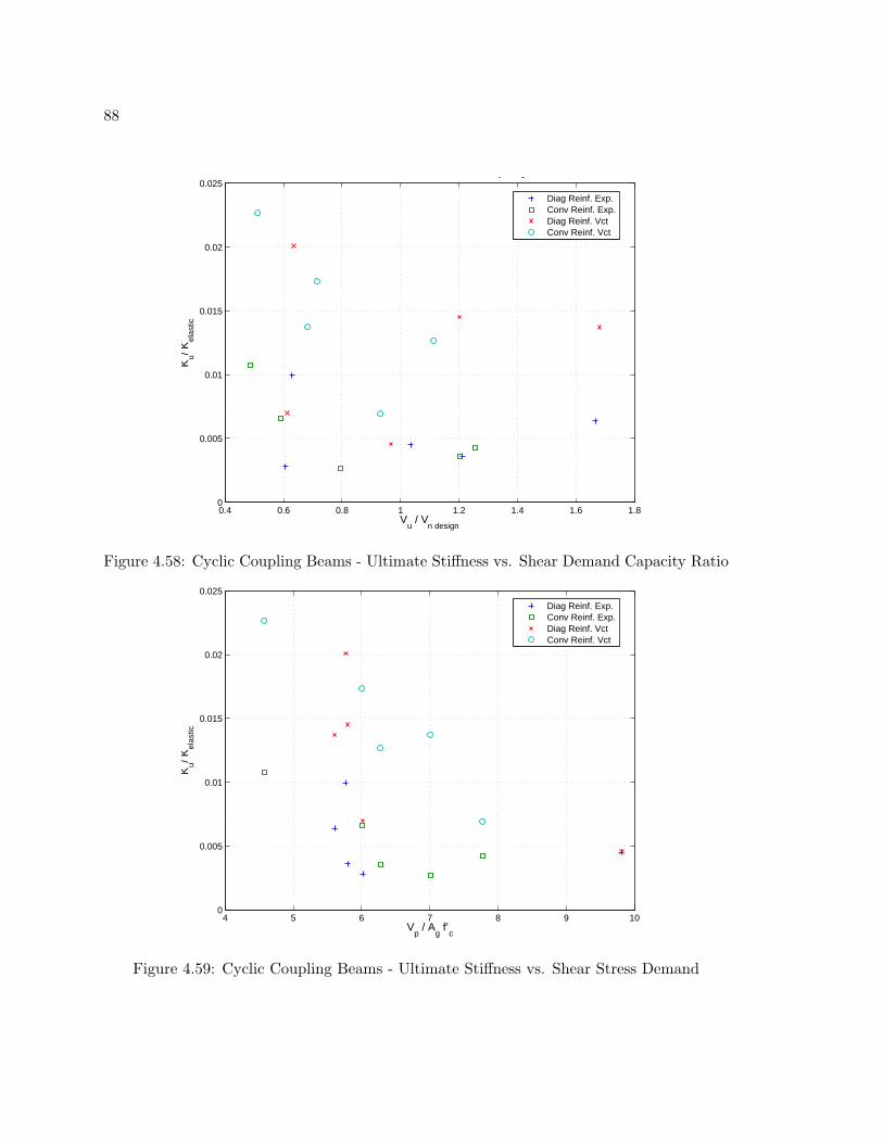
88
0.4 0.6 0.8 1 1.2 1.4 1.6 1.80
0.005
0.01
0.015
0.02
0.025
Vu / V
n design
Ku/ K
elas
tic
Cyclic Coupling BeamsUltimate Stiffness vs Shear Demand Capacity Ratio
Diag Reinf. Exp.Conv Reinf. Exp.Diag Reinf. VctConv Reinf. Vct
Figure 4.58: Cyclic Coupling Beams - Ultimate Stiffness vs. Shear Demand Capacity Ratio
4 5 6 7 8 9 100
0.005
0.01
0.015
0.02
0.025
Vp / A
g f’
c
Ku/ K
elas
tic
Cyclic Coupling BeamsUltimate Stiffness vs Shear Stress Demand
Diag Reinf. Exp.Conv Reinf. Exp.Diag Reinf. VctConv Reinf. Vct
Figure 4.59: Cyclic Coupling Beams - Ultimate Stiffness vs. Shear Stress Demand

89
4.7 Discussion and Comparison of Results
Comparison of simulation and experimental data indicates that Vector2 can provide a good
prediction of the behavior through the yield point and up to the ultimate strength; however,
it generally underestimates the ultimate displacement of the specimens. The analytical
models were able to predict the yield strength with an average error of 5% over strength
and the ultimate strength with an average error of only 2% under strength. The analytical
model provides a fairly good prediction of yield displacement, typically under predicting it
by 11%. However, the model greatly under predicts ultimate displacement; the predicted
values were, on average, 42% of the experimental values.
In general, the analytical specimens have a higher stiffness prior to yield and reach
the maximum load early in the load sequence, whereas the experimental results tend to
gradually approach the maximum load near the end of the displacement history. The
increased stiffness of the model is due, in part, to the assumption of perfect bond between
the reinforcing bars and the concrete. In the experimental specimens, flexural cracks would
gradually open and bond-slip of the main reinforcing bars would occur. The opening of
flexural cracks and the slip of the reinforcing bars provide a significant contribution to
the lateral deflections of the coupling beam and thus reduce the effective stiffness. The
premature failure of the model occurs when an extreme fiber crushes and the model cannot
simulate the redistribution of the loads. The crushed element cannot support any load and
forces a concentration of stress in the next element, causing a rapid progression of failure
through the specimen.
With the modeling parameters and analysis capabilities of Vector2 understood, the pre-
dictive analysis of the NEESR coupling beams could be completed with an adequate level
of confidence.

90
4.8 Model Parameter Study
4.8.1 Vecchio and Palermo Parameters
After the completion of the experimental coupling beam models a report detailing the use of
VecTor2 to model the behavior of planar shear walls was published by Vecchio and Palermo
(2007). This report utilized a slight variation on the set of constitutive models used, the
author felt it would be prudent to see if the settings used by Vecchio and Palermo could
improve the behavior of the coupling beam models. The Zhao MCB2 specimen was chosen
for this study because it showed a post-elastic behavior that did not match the reported
experimental data. In addition to these settings, the model was also rerun with a smaller
convergence criteria and an increased number of iterations per displacement step.
The Vecchio settings differ in the following areas. The compression softening model
used was Vecchio 1992-A (e1/e2-Form), this is a strength and strain softening model vs.
the strength only softening model previously used. Tension Softening and Rebar Dowel
Action were not considered.
Figure 4.60 shows a comparison between the base model and the Vecchio settings. The
settings used by Vecchio provide the same performance up to the peak strength and a slight
increase in displacement ductility after the peak was reached. The improvement in post-
peak performance was nominal and did not provide a large enough improvement to warrant
a re-modeling of all the experimental coupling beam specimens.
Figure 4.61 shows a comparison of between the base model and the with an increased
iteration allowance. The two results are essentially identical, showing that the maximum of
100 iterations per displacement step is sufficient to provide convergence.

91
0 10 20 30 40 50 60 70 800
50
100
150
200
250
300
350
400
She
ar (
KN
)
Displacement (mm)
Zhao MCB2 ComparissonsBase Model vs. Vecchio Settings
ExperimentalVecTor2 − BaseVecTor2 − Vecchio
Figure 4.60: Zhao MCB2 Model Comparisons
0 10 20 30 40 50 60 70 800
50
100
150
200
250
300
350
400
She
ar (
KN
)
Displacement (mm)
Zhao MCB2 ComparissonsBase Model vs. Increased Iterations
ExperimentalVecTor2 − BaseVecTor2 − Iter.
Figure 4.61: Zhao MCB2 Model Comparisons

92
Chapter 5
EVALUATION OF TRANSVERSE REINFORCEMENT OFCOUPLING BEAMS
5.1 Introduction
The primary objective of this section was to determine the effect of transverse reinforce-
ment, or confinement, on the performance of diagonally reinforced coupling beams. The
performance of a coupling beam with code compliant transverse reinforcement was com-
pared to three different transverse confinement configurations. Additionally, the effects of
the adjacent slab reinforcement on the coupling beam were investigated.
Discussions with an external advisory board (Hooper, Hawkins, etc. 2006) indicate that
current code requirements often result in diagonally reinforced coupling beams that have
highly congested transverse reinforcement resulting in difficult and expensive construction.
A revision to the current code confinement methods has been proposed by ACI committee
318H; the proposal will allow for greater transverse reinforcement spacing and introduce an
alternative design procedure that will allow for a less congested transverse reinforcement
configuration.
5.1.1 Approach
Nonlinear finite element analysis using VecTor2 were completed to simulate the performance
of the coupling beam variations when subjected to in-plane displacements. The design
of the coupling beam from the coupled wall model discussed in Chapter 6 was used as
the reference design (in terms of dimensions, materials, and diagonal reinforcement). The
analysis assumptions determined in Chapter 4 were used for each of the coupling beam
models explored.

93
5.1.2 Organization of Chapter
The following provides a brief outline of this chapter.
Section 5.2 describes the current and proposed design requirements.
Section 5.3 describes the different coupling beam models and their confinement variations.
Section 5.4 discusses the finite element modeling techniques.
Section 5.5 discusses how the analysis results were compared to the reference model.
Section 5.6 discusses the simulation results from the VecTor2 finite element analysis.
Section 5.7 compares the overall performance of the confinement variations.
5.2 Design Requirements
5.2.1 ACI 318-05 Current Code
The current ACI 318 code specifies that diagonal reinforcement must be used in coupling
beams with aspect ratio, ln/d, that is less than two or with factored shear force Vu exceeding
4√
f ′cbwd. Additional confinement is required on the diagonal reinforcement per §21.7.7.4.
The confinement requirement adopts §21.4.4, transverse reinforcement for columns in Special
Moment Resistant Frames, including the following limits
• §21.4.4.1 Area of transverse reinforcement shall not be less than:
Ash = 0.3(sbcf′c/fyt)(Ag/Ach − 1) Equation (21-3)
Ash = 0.09sbcf′c/ft Equation (21-4)
• §21.4.4.2 Spacing of transverse reinforcement shall not exceed the smallest of (a), (b),
and (c):
(a) one-quarter of the minimum member dimension;

94
(b) six times the diameter of the longitudinal reinforcement; and
(c) so = 4 + 14−hx3
For diagonally reinforced coupling beams, the “member” is defined as cross section of the
diagonal bar cage (out to out) plus the nominal cover dimension.
5.2.2 ACI 318H-CH047d Proposal
ACI Committee 318H has submitted proposal CH047 which seeks to modify the transverse
reinforcement requirements for diagonally reinforced coupling beams. It is likely that this
proposal will be incorporated into the next revision of ACI 318, set to be published in 2008.
The proposal is separated into two sections; a revision to the current spacing limits and an
alternative confinement method. The first section changes the spacing requirements of the
transverse reinforcement by removing the “one-quarter of the minimum member dimension”
requirement. The second section introduces an alternative design method that will allow the
entire coupling beam to be enclosed in transverse reinforcement satisfying the requirements
of §21.4.4.1(b) and (c), and §21.4.4.2, except for Equation (21-3) and the spacing of cross-
ties or legs in the plane of the cross section of the coupling beam shall not exceed 8 inches.
Equation (21-3) defines the required area of transverse reinforcement based on a ratio of
the confined core to the gross area of the member; it is specifically applicable to column
sections and need not apply to diagonal bar groups. In summary, the alternative design
method will allow the entire coupling beam to be confined rather than just the diagonal
bar groups provided the transverse reinforcement meet the same requirements as currently
specified in the ACI 318-05 code less with the additional spacing limit on cross tie spacing.
5.3 Description of Models
Five different coupling beam confinement options were explored; the first model was de-
signed to meet the current ACI code, the second model was intended to represent the effect
of additional top steel from the adjacent slab and/or collector elements, the third and fourth

95
models are based on the ACI 318H-CH047 proposal, the fifth model introduces a modified
ACI 318H-CH047 proposal with one half the confinement reinforcement.
The coupling beam confinement was designed at full scale and the resulting reinforcement
ratios applied to the one-third scale models, allowing the models to better reflect full scale
applications. The reinforcement ratios of the coupling beam models are shown in Table 5.1,
tie spacing and ties sizes are approximate based on the one-third scale model. Each of the
coupling beam variations is described in detail in the following sections.
5.3.1 CBR-ACI: ACI318-05 Reference Model
This model was designed to meet the current ACI 318-05 code. Confinement was provided
around each diagonal bar group by #2 ties @ 1” o.c. Additional nominal reinforcement
consists of 2 #2 bars top and bottom plus 1 #2 on each face. Nominal #2 stirrups at 6”
o.c. are provided around the entire beam. The tie spacing around the diagonal bar groups
was controlled by the one quarter of the member dimension limit in §21.4.4.2(a).
5.3.2 CBR-ACI-S: Reference model with additional slab steel
This model contains the same reinforcement as the CBR-ACI base model, except for addi-
tional top steel to simulate the contribution of the slab reinforcement and/or collector steel
as is often seen in typical building construction.
5.3.3 CBR-318H: Confinement to meet the ACI 318H proposal
This model was designed to meet the reduced spacing proposal. The spacing of the ties
around each diagonal bar group can be increased to 1 1/2” due to the removal of the one
quarter of the member dimension spacing limit. Tie spacing was controlled by the area
of steel required, Ash. Additional reinforcement and nominal ties remain the same as the
reference model.

96
Table 5.1: Coupling Beam Confinement Variations
ρl ρv ρt Ad ρdv ρdt
Model (As/db) (Av/sb) (At/ds) (mm2) (Adt/dcst) (Adt/bcst)CBR-ACI 0.31% 0.27% 0.10% 516.1 1.63% 3.27%CBR-ACI-S 0.31%* 0.27% 0.10% 516.1 1.63% 3.27%CBR-318H 0.31% 0.27% 0.10% 516.1 1.09% 2.18%CBR-318H-F 0.42% 0.74% 0.74% 516.1 - -CBR-318H-M 0.28% 0.56% 0.35% 516.1 - -* plus additional top steel of 194.8 mm2
5.3.4 CBR-318H-F: Confinement of the entire section to meet ACI 318H proposal
This model was designed to meet the proposed alternative detailing methods. The entire
beam was confined by stirrups with both vertical and horizontal cross ties. Tie spacing
was controlled by the one quarter of the member dimension requirement, while the area
and number of cross ties was controlled by the Ash requirement and the maximum spacing
between cross ties.
5.3.5 CBR-318H-M: Confinement of the entire section with reduced trans. reinf.
The confinement of this model is based on a reduced Ash requirement. Ash was reduced by
half to 0.045sbcf′c/fy. The tie spacing limits as proposed in ACI 318H-CH047 are used.
5.4 Finite Element Modeling
The finite element model for the coupling beams uses the same constitutive models and
analysis parameters as previously discussed in Chapter 4. The diagonal reinforcement in
all models and the slab steel in CBR-ACI-S were modeled with discrete truss-bar elements.
The material properties are shown in Table 5.2.
The coupling beams were simulated both monotonically and cyclically. The monotonic
simulations were continued until significant strength loss occurred or the model became
numerically unstable. The cyclic simulations had three repetitions per cycle with increasing

97
Table 5.2: Coupling Beam Material Properties
Concrete Reinforcementf
′c 5.0 ksi fy 60 ksi
ft 0.50 ksi fu 90 ksiEc 4030 ksi Es 29000 ksiε0 0.003 Esh 170 ksi
εsh 0.010
magnitude per cycle, to the approximate yield displacement (δy), 2δy, 4δy, 6δy. If the models
had not failed at 6δy, they were then pushed monotonically to failure. Monotonic model
names are preceded with an “M”, i.e. MCBR-ACI is the monotonically loaded version of
CBR-ACI.
5.5 Description of Evaluation Method
The analysis results from each of the coupling beam simulation was evaluated to determine
the predicted mechanisms of deformation, initial reinforcement yielding, ultimate strength,
loss of stiffness, and loss of strength. The studied response parameters include:
Vy: shear observed in the coupling beam at first yield of diagonal bars.
Vu: maximum shear observed in the coupling beam.
V1.5%: shear in the coupling beam at 1.5% drift.
V6.0%: shear in the coupling beam at 6.0% drift.
Ky: secant stiffness at the first yield of the diagonal bars.
Ku: secant stiffness at the ultimate shear strength.
K1.5% : secant stiffness corresponding to 1.5% drift in the coupling beam.

98
K6.0%: secant stiffness corresponding to 6.0% drift in the coupling beam.
δy: displacement at the first yield of the diagonal bars.
δu: displacement at the maximum predicted shear.
∆y: drift in the coupling beam at the first yield of the diagonal bars, δy/L.
∆u: drift in the coupling beam at the maximum predicted shear, δu/L.
∆0.85Vu: drift in the coupling beam when 85% of the predicted maximum strength, Vu, was
reached.
µu: displacement ductility at the maximum predicted shear, δu/δy.
5.6 Simulation Results
The VecTor2 simulation results and load-drift response plots are discussed in the following
sections.
5.6.1 Load Drift Plots
Load-drift plots for all models are shown in Figures 5.1 to 5.10. The load-drift plots have
been annotated to show the locations of initial yield and ultimate shear strength. The
design shear strength, Vn = 50kips, calculated using the ACI 318 code method, is shown
on the load-drift plots with a dotted line.
Some of the cyclic simulations show results that are “jagged” at the higher displacement
cycles. The jaggedness of the load-drift results are due to incomplete convergence within
VecTor2. The convergence criteria was limited to one hundred iterations, and thus did not
allow the model to completely converge at every displacement step. The “jagged” portions
of the curve can be assumed to fluctuate around the correct solution, however, the lack of
convergence is an indication that some elements may be highly stressed or distorted.

99
0 1 2 3 4 5 6 7 8 90
10
20
30
40
50
60
70
80
90
100
She
ar (
Kip
)
Drift (%)
Vy
Vu
Vn
VecTor2
Figure 5.1: MCBR-ACI Load-Drift Response
−8 −6 −4 −2 0 2 4 6 8−100
−80
−60
−40
−20
0
20
40
60
80
100
She
ar (
Kip
)
Drift (%)
VyVu
Vy
Vu
Vn
VecTor2
Figure 5.2: CBR-ACI Load-Drift Response

100
0 1 2 3 4 5 6 7 8 90
10
20
30
40
50
60
70
80
90
100S
hear
(K
ip)
Drift (%)
Vy
Vu
Vn
VecTor2
Figure 5.3: MCBR-ACI-S Load-Drift Response
−8 −6 −4 −2 0 2 4 6 8−100
−80
−60
−40
−20
0
20
40
60
80
100
She
ar (
Kip
)
Drift (%)
VyVu
Vy
VuV
n
VecTor2
Figure 5.4: CBR-ACI-S Load-Drift Response

101
0 1 2 3 4 5 6 7 8 90
10
20
30
40
50
60
70
80
90
100
She
ar (
Kip
)
Drift (%)
Vy
Vu
Vn
VecTor2
Figure 5.5: MCBR-318H Load-Drift Response
−8 −6 −4 −2 0 2 4 6 8−100
−80
−60
−40
−20
0
20
40
60
80
100
She
ar (
Kip
)
Drift (%)
VyVu
Vy
Vu
Vn
VecTor2
Figure 5.6: CBR-318H Load-Drift Response
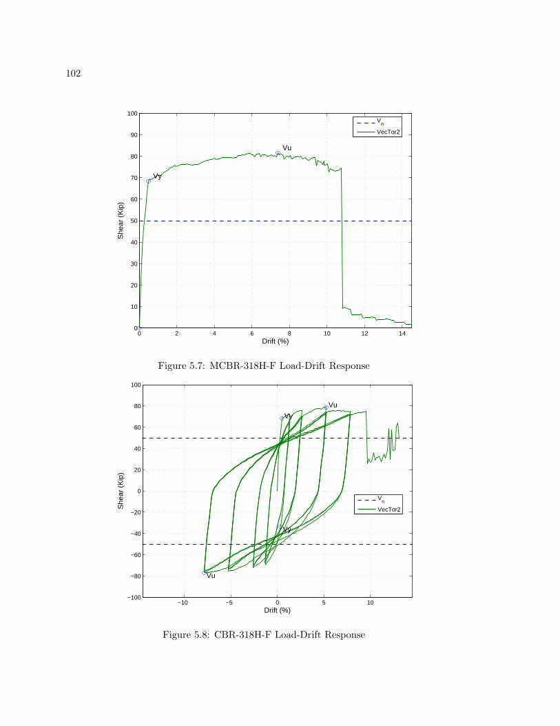
102
0 2 4 6 8 10 12 140
10
20
30
40
50
60
70
80
90
100S
hear
(K
ip)
Drift (%)
Vy
Vu
Vn
VecTor2
Figure 5.7: MCBR-318H-F Load-Drift Response
−10 −5 0 5 10−100
−80
−60
−40
−20
0
20
40
60
80
100
She
ar (
Kip
)
Drift (%)
Vy
Vu
Vy
Vu
Vn
VecTor2
Figure 5.8: CBR-318H-F Load-Drift Response

103
0 2 4 6 8 10 12 140
10
20
30
40
50
60
70
80
90
100
She
ar (
Kip
)
Drift (%)
Vy
Vu
Vn
VecTor2
Figure 5.9: MCBR-318H-M Load-Drift Response
−10 −5 0 5 10−100
−80
−60
−40
−20
0
20
40
60
80
100
She
ar (
Kip
)
Drift (%)
Vy
Vu
Vy
Vu
Vn
VecTor2
Figure 5.10: CBR-318H-M Load-Drift Response

104
Table 5.3: Coupling Beam Stiffness Results
Model Ky ∆Ref Ku ∆Ref K1.5% ∆Ref K6.0% ∆Ref
MCBR-ACI 455.9 0.00% 57.7 0.00% 185.9 0.00% 48.1 0.00%
MCBR-ACIS 546.6 19.91% 68.4 18.56% 196.6 5.74% 51.6 7.28%
MCBR-318H 465.9 2.20% 75.9 31.62% 187.9 1.06% 46.2 -3.77%
MCBR-318H-F 579.4 27.09% 46.0 -20.17% 207.3 11.51% 55.5 15.42%
MCBR-318H-M 545.6 19.70% 48.6 -15.71% 188.2 1.23% 51.3 6.68%
Average 518.7 13.78% 59.3 2.86% 193.1 3.91% 50.5 5.12%
CBR-ACI 401.3 0.00% 60.5 0.00% 173.9 0.00% - -
CBR-ACIS 546.6 36.22% 44.6 -26.26% 181.0 4.09% 46.6 -
CBR-318H 406.1 1.20% 61.9 2.21% 172.9 -0.57% - -
CBR-318H-F 580.0 44.54% 62.5 3.26% 195.1 12.23% 51.9 -
CBR-318H-M 545.9 36.02% 43.1 -28.84% 177.3 1.98% 49.2 -
Average 496.0 23.60% 54.5 -9.93% 180.0 3.55% 49.2 -
Stiffness (K) in K-in
∆Ref : percentage change relative to reference model
5.6.2 Stiffness
The secant stiffness of the coupling beams was calculated at yield, ultimate shear, 1.5% drift,
and 6.0% drift and is summarized in Table 5.3. The average yield stiffness and ultimate
stiffness are 507.3 and 56.9 K-in respectively. However, separating the couplings beams with
ACI confinement (CBR-ACI, CBR-318H and CBR-ACI-S) from those with the proposed
full confinement (CBR-318H-F and CBR-318H-M) shows that the ACI coupling beams have
a lower average yield stiffness of 432.3 k-in and a higher average ultimate stiffness of 64.0
k-in, while the full confinement beams have a higher average yield stiffness of 562.7 k-in
and a lower average ultimate stiffness of 50.0 k-in. The full confinement method results in
a 23% higher yield stiffness and a 28% lower ultimate stiffness than the ACI confinement
method.
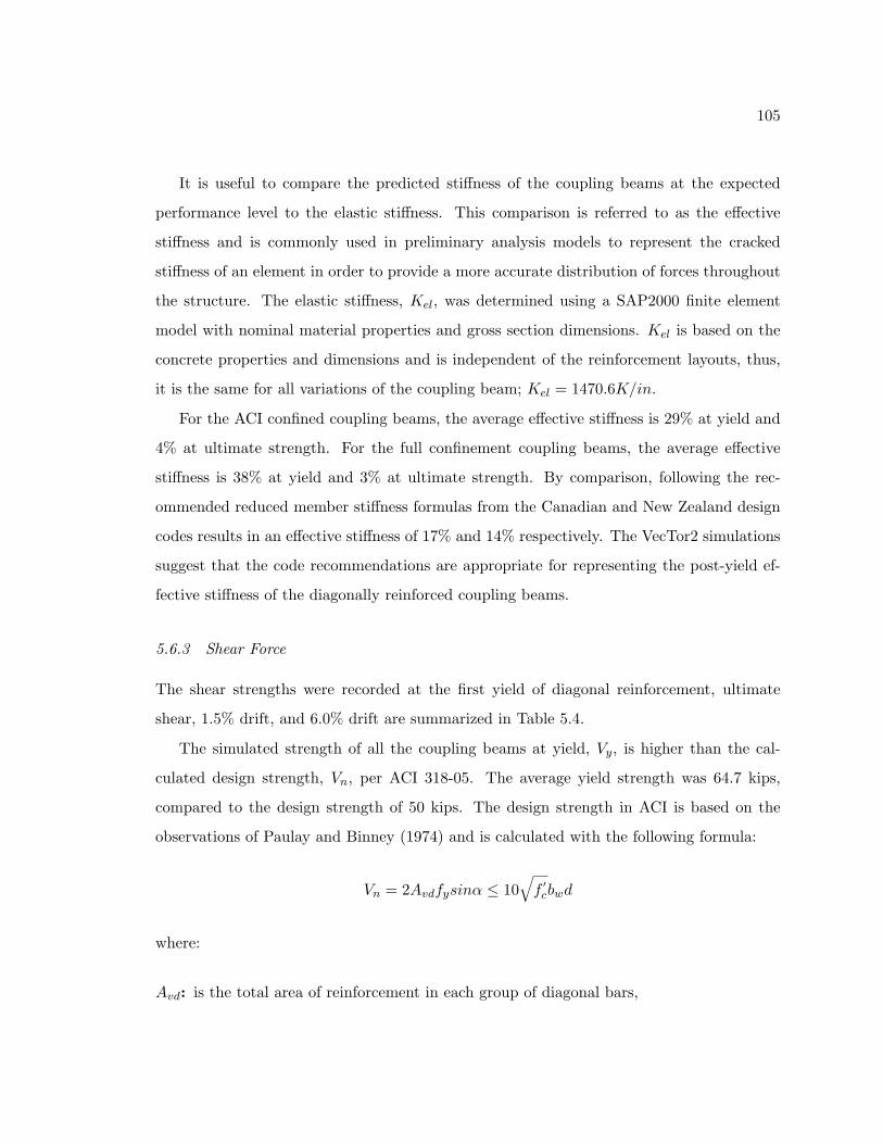
105
It is useful to compare the predicted stiffness of the coupling beams at the expected
performance level to the elastic stiffness. This comparison is referred to as the effective
stiffness and is commonly used in preliminary analysis models to represent the cracked
stiffness of an element in order to provide a more accurate distribution of forces throughout
the structure. The elastic stiffness, Kel, was determined using a SAP2000 finite element
model with nominal material properties and gross section dimensions. Kel is based on the
concrete properties and dimensions and is independent of the reinforcement layouts, thus,
it is the same for all variations of the coupling beam; Kel = 1470.6K/in.
For the ACI confined coupling beams, the average effective stiffness is 29% at yield and
4% at ultimate strength. For the full confinement coupling beams, the average effective
stiffness is 38% at yield and 3% at ultimate strength. By comparison, following the rec-
ommended reduced member stiffness formulas from the Canadian and New Zealand design
codes results in an effective stiffness of 17% and 14% respectively. The VecTor2 simulations
suggest that the code recommendations are appropriate for representing the post-yield ef-
fective stiffness of the diagonally reinforced coupling beams.
5.6.3 Shear Force
The shear strengths were recorded at the first yield of diagonal reinforcement, ultimate
shear, 1.5% drift, and 6.0% drift are summarized in Table 5.4.
The simulated strength of all the coupling beams at yield, Vy, is higher than the cal-
culated design strength, Vn, per ACI 318-05. The average yield strength was 64.7 kips,
compared to the design strength of 50 kips. The design strength in ACI is based on the
observations of Paulay and Binney (1974) and is calculated with the following formula:
Vn = 2Avdfysinα ≤ 10√
f ′cbwd
where:
Avd: is the total area of reinforcement in each group of diagonal bars,

106
fy: is the yield strength of the diagonal reinforcement,
α: is the angle between the diagonally placed bars and the longitudinal axis of the coupling
beam,
f′c: is the compressive strength of the concrete,
bw: is the width of the beam, and
d: is the distance from the extreme compression fiber to the centroid of the longitudinal
tension reinforcement.
Paulay and Binney’s research suggested a method for calculating the ultimate capacity of a
diagonally reinforced coupling beam based on the assumption that after first yielding and
load reversal the diagonal reinforcement will resist all the forces. Following this assumption,
the shear resistance is the sum of the vertical force components of the diagonal bar in
tension and in compression. At the ultimate strength it is assumed that the bars will be
fully stressed in tension and compression, thus leading to the above formula for strength.
The ACI code has assumed that the reinforcement does not gain any strength after yield;
an elastic-perfectly-plastic steel model. This assumption allows the ultimate shear strength
calculation of Paulay and Binney to apply at the yield point, and to be used as the design
strength.
The following illustration of internal forces and moments are taken from the simulation
of model CRB-ACI, however the resulting trend is similar for all the models. The VecTor2
simulations show that, at yield, the internal forces are not the same as the internal force
mechanisms Paulay and Binney proposed for the ultimate state. At the yield point, the
diagonal bars in tension have yielded, however the diagonal bars in compression are at
approximately 95% of yield. At subsequent load cycles, the stress level in the compression
bars continue to lag behind the tension bars by an average of 3 to 5%. At the displacement
step where the tension bar reaches the yield stress, the tensile stress ends up being slightly

107
Table 5.4: Coupling Beam Strength Results
Model Vy ∆Ref Vu ∆Ref V1.5% ∆Ref V6.0% ∆Ref
MCBR-ACI 62.5 0.00% 71.4 0.00% 65.8 0.00% 70.0 0.00%
MCBR-ACIS 64.5 3.28% 76.7 7.36% 69.6 5.74% 75.1 7.29%
MCBR-318H 63.8 2.19% 70.1 -1.85% 66.5 1.06% 67.3 -3.76%
MCBR-318H-F 68.4 9.46% 81.5 14.11% 73.4 11.52% 80.8 15.42%
MCBR-318H-M 64.4 3.11% 76.5 7.08% 66.6 1.23% 74.6 6.69%
Average 64.7 3.61% 75.3 5.34% 68.4 3.91% 73.5 5.13%
CBR-ACI 62.9 0.00% 71.4 0.00% 61.5 0.00% - -
CBR-ACIS 64.4 2.38% 73.8 3.26% 64.1 4.20% 67.9 -
CBR-318H 63.7 1.24% 70.6 -1.20% 61.2 -0.55% - -
CBR-318H-F 68.3 8.53% 78.7 10.16% 69.1 12.31% 75.6 -
CBR-318H-M 64.3 2.18% 74.6 4.40% 62.8 2.08% 71.7 -
Average 64.7 2.87% 73.8 3.32% 63.7 3.61% 71.7 -
Strength (V) in Kips
∆Ref : percentage change relative to reference model
higher than 60 ksi while the stress in the compression bar is slightly lower than 60 ksi. As a
result, the combined shear strength of the two diagonal bars matches the theoretical value
calculated using the Paulay and Binney method. However, the strength of the diagonal
bars only accounts for approximately 75% of the overall shear capacity of the coupling
beam. Additional shear demand is developed by the flexural response of the beam through
tensile yielding of the longitudinal reinforcement and compressive stress in the concrete.
The moment developed by this couple has to be balanced by shear forces in the vertical
reinforcement and shear stress in the concrete; this additional shear force accounts for the
remaining 25% of the shear strength of the coupling beam. The coupling beams never reach
the theoretical point where all of the resistance is provided by the diagonal reinforcement,
there is always a contribution from the vertical reinforcement.
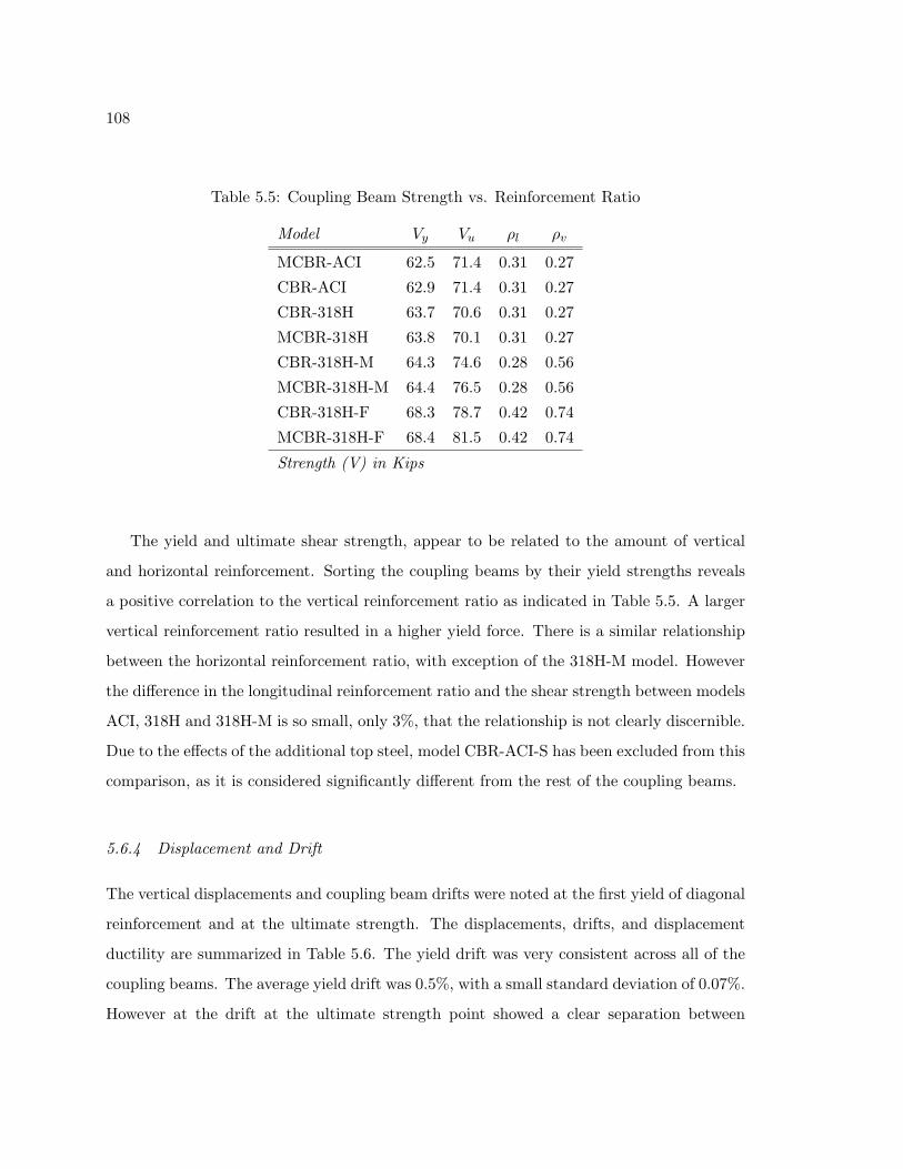
108
Table 5.5: Coupling Beam Strength vs. Reinforcement Ratio
Model Vy Vu ρl ρv
MCBR-ACI 62.5 71.4 0.31 0.27
CBR-ACI 62.9 71.4 0.31 0.27
CBR-318H 63.7 70.6 0.31 0.27
MCBR-318H 63.8 70.1 0.31 0.27
CBR-318H-M 64.3 74.6 0.28 0.56
MCBR-318H-M 64.4 76.5 0.28 0.56
CBR-318H-F 68.3 78.7 0.42 0.74
MCBR-318H-F 68.4 81.5 0.42 0.74
Strength (V) in Kips
The yield and ultimate shear strength, appear to be related to the amount of vertical
and horizontal reinforcement. Sorting the coupling beams by their yield strengths reveals
a positive correlation to the vertical reinforcement ratio as indicated in Table 5.5. A larger
vertical reinforcement ratio resulted in a higher yield force. There is a similar relationship
between the horizontal reinforcement ratio, with exception of the 318H-M model. However
the difference in the longitudinal reinforcement ratio and the shear strength between models
ACI, 318H and 318H-M is so small, only 3%, that the relationship is not clearly discernible.
Due to the effects of the additional top steel, model CBR-ACI-S has been excluded from this
comparison, as it is considered significantly different from the rest of the coupling beams.
5.6.4 Displacement and Drift
The vertical displacements and coupling beam drifts were noted at the first yield of diagonal
reinforcement and at the ultimate strength. The displacements, drifts, and displacement
ductility are summarized in Table 5.6. The yield drift was very consistent across all of the
coupling beams. The average yield drift was 0.5%, with a small standard deviation of 0.07%.
However at the drift at the ultimate strength point showed a clear separation between

109
Table 5.6: Coupling Beam Drift Results
Model ∆y ∆Ref ∆u ∆Ref µu ∆Ref ∆0.85Vu
MCBR-ACI 0.57% 1.0 5.16% 1.0 8.9 1.0 6.90%
MCBR-ACIS 0.49% 0.9 4.68% 0.9 9.3 1.1 9.00%
MCBR-318H 0.57% 1.0 3.85% 0.7 6.6 0.7 7.40%
MCBR-318H-F 0.49% 0.9 7.38% 1.4 14.8 1.7 10.75%
MCBR-318H-M 0.49% 1.0 6.56% 1.0 13.1 1.0 12.97%
Average 0.52% 0.9 5.53% 1.0 10.5 1.1 9.40%
CBR-ACI 0.65% 1.3 4.92% 0.8 7.4 0.6 5.21%
CBR-ACIS 0.49% 1.0 6.89% 1.1 13.8 1.1 -
CBR-318H 0.65% 1.3 4.75% 0.7 7.1 0.5 5.18%
CBR-318H-F 0.49% 1.0 5.25% 0.8 10.5 0.8 9.49%
CBR-318H-M 0.49% 1.0 7.22% 1.1 14.4 1.1 -
Average 0.55% 1.1 5.81% 0.9 10.6 0.8 6.63%
∆Ref : percentage change relative to reference model

110
the ACI confinement and the full confinement methods. The coupling beams with ACI
confinement had an average ultimate drift of 4.7% while the average for the full confinement
coupling beams was 6.6%. These ultimate displacements result in an average displacement
ductility of 7.5 for the ACI confinement and and 13.2 for the full confinement method.
These results suggest that the full confinement method can provide better confinement of
the coupling beam and allow it to behave in a more ductile manner in the post-yield region.
5.7 Comparison of Confinement Variations
5.7.1 CBR-ACI vs. CBR-318H
Figure 5.11 shows a comparison between the monotonic load-drift response of the refer-
ence model , (MCBR-ACI), and the reduced tie spacing model, (MCBR-318H). Figure 5.12
shows a similar comparison between the cyclic simulations. The ACI 318H-CH047 reduced
spacing proposal, model ACI-318H, shows only a slight reduction in displacement ductil-
ity and provides essentially the same ultimate strength capacity. These results suggest
that the reduced spacing requirements can provide equivalent confinement of the diagonal
reinforcement to that of the current ACI specifications with only a minimal reduction in
displacement ductility capacity at the point when the shear force drops below 85% of Vu in
the monotonic simulations. The cyclic simulations do not show any significant reduction in
displacement or shear force capacity.

111
0 1 2 3 4 5 6 7 8 90
10
20
30
40
50
60
70
80
90
100
She
ar (
Kip
)
Drift (%)
Vpr
MCBR−ACIMCBR−318H
Figure 5.11: MCBR-ACI vs. MCBR-318H Load-Drift Response
−8 −6 −4 −2 0 2 4 6 8−100
−80
−60
−40
−20
0
20
40
60
80
100
She
ar (
Kip
)
Drift (%)
Vpr
CBR−ACICBR−318H
Figure 5.12: CBR-ACI vs. CBR-318H Load-Drift Response

112
5.7.2 CBR-ACI vs CBR-318H-F
Figure 5.13 shows a comparison between the monotonic load-drift response of the reference
model , (MCBR-ACI), and the full confinement model, (MCBR-318H-F). Figure 5.14 shows
a similar comparison between the cyclic simulations.
The ACI 318H-CH047 full confinement proposal, model ACI-318H-F, shows a significant
increase in yield strength, ultimate strength, and displacement ductility when compared to
the base ACI design. In addition to the increased displacement ductility, the VecTor2 output
was much smoother at larger deformations than that of the ACI design. The increase in
displacement ductility and stability of the model can be attributed increased area of fully
confined concrete. Confining the whole section results in a larger spread of the tensile strains
and increased crack distribution over the entire coupling beam, as shown in the comparison
of the crack patterns at 5.25% drift (the ultimate drift capacity of M+CBR-ACI) of both
models in Figures 5.15 and 5.16.
The increase in yield and ultimate strength can be attributed to the increase in both
vertical and horizontal reinforcement ratios, as discussed in Section 5.6.3. While this may
seem a welcome improvement, use of full confinement on coupling beams in performance-
based designs should be used cautiously until a reliable method for predicting the actual
strength can be developed.

113
0 2 4 6 8 10 12 140
10
20
30
40
50
60
70
80
90
100
She
ar (
Kip
)
Drift (%)
Vpr
MCBR−ACIMCBR−318H−F
Figure 5.13: MCBR-ACI vs. MCBR-318H-F Load-Drift Response
−8 −6 −4 −2 0 2 4 6 8−100
−80
−60
−40
−20
0
20
40
60
80
100
She
ar (
Kip
)
Drift (%)
Vpr
CBR−ACICBR−318H−F
Figure 5.14: CBR-ACI vs. CBR-318H-F Load-Drift Response

114
Figure 5.15: CBR-ACI Crack Distribution at 5.25 % drift
Figure 5.16: CBR-318H-F Crack Distribution at 5.25 % drift

115
5.7.3 CBR-ACI and CBR-318H-M
Figure 5.17 shows a comparison between the monotonic load-drift response of the refer-
ence model, (MCBR-ACI), and the modified full confinement model, (MCBR-318H-M).
Figure 5.18 shows a similar comparison between the cyclic simulations. The strength of
model MCBR-318H-M begins to degrade at approximately 7.3% drift due to crushing of
the concrete at the ends of the coupling beam. The shear stress capacity is reduced and
the model begins to loose shear force, then at 8.33% drift the shear force begins to increase
again as the tensile stress in the diagonal reinforcement continues to strain harden.
The two models have nearly the same response up to the yield point and both yield at
a very similar force (62.5 and 64.4 kips), however the full confined model (MCBR-318H-M)
continues to gain strength and is able to undergo nearly twice the deformation. Both models
have the same diagonal reinforcement and have very similar longitudinal reinforcement ratios
(0.31% vs. 0.28%), thus resulting in their similar yield strength. The full confinement of
model MCBR-318H-M allows the model to undergo larger displacements than the reference
specimen which allows the diagonal reinforcement to reach higher strains and results in a
larger ultimate shear force. The increase in the vertical reinforcement also allows for the
cracking to be well distributed throughout the model, as discussed in the previous section.
5.8 Conclusions
VecTor2 simulations of the coupling beam confinement variations supports the following
conclusions.
• The VecTor2 simulations suggest that an effective stiffness between approximately 5%
and 30% would be appropriate to use in an elastic model to represent the post-yield
stiffness of diagonally reinforced coupling beams. A decision to use a lower effective
stiffness should be used with the understanding that it represents a higher level of
expected damage to the coupling beam.
• The ACI 318H-CH047 proposed revision to the spacing requirements on the closed

116
0 2 4 6 8 10 12 140
10
20
30
40
50
60
70
80
90
100S
hear
(K
ip)
Drift (%)
Vpr
MCBR−ACIMCBR−318H−M
Figure 5.17: MCBR-ACI vs. MCBR-318H-M Load-Drift Response
−8 −6 −4 −2 0 2 4 6 8−100
−80
−60
−40
−20
0
20
40
60
80
100
She
ar (
Kip
)
Drift (%)
Vpr
CBR−ACICBR−318H−M
Figure 5.18: CBR-ACI vs. CBR-318H-M Load-Drift Response

117
ties around the diagonally placed reinforcement will have a negligible effect on the
performance of the coupling beam. It is capable of providing an adequate level of con-
finement so as to allow the coupling beam to reach essentially the same displacement
ductility and shear strength as the current ACI 318-05 specifications.
• The ACI 318H-047 full confinement proposal results in a 9% average increase in the
shear strength at yield and a 12% average increase in the ultimate strength. It in-
creases the average drift from 4.67% to 6.60% resulting in an increase in 76% increase
in the displacement ductility from 7.5 to 13.2. VecTor2 simulations of coupling beams
designed to meet the ACI 318H-CH047 proposal suggests that the performance of
diagonally reinforced coupling beams can be improved by providing full confinement
of the entire section.
• The ACI method for calculating the shear strength of a diagonally reinforced coupling
beams tends to be less than that predicted using VecTor2 finite element simulations.
The ACI method notes that the “diagonally placed bars shall be considered to con-
tribute to Mn of the coupling beam”, indicating that the flexural strength of the
coupling beam is affected by both the longitudinal and diagonal reinforcement. How-
ever, only the diagonal reinforcement is allowed to be used in calculating the shear
strength of the coupling beam, resulting in an under-estimation of the true strength of
the beam. The intent of these specifications is to ensure that the diagonally reinforced
coupling beams will be flexural controlled, however it is not specified that the shear
strength be checked against the plastic shear demand of Vp = 2Mp/L.
• The ACI 318H-CH047 full confinement proposal will result in coupling beams with
higher longitudinal and vertical reinforcement ratios in order to meet the confinement
and spacing requirements. While this additional steel will provide confinement of the
entire section, it will also increase the flexural and shear strength of the coupling
beam. Before this proposal is improved the method for calculating the shear strength

118
needs to be revised to reflect the shear strength due to the additional reinforcement.

119
Chapter 6
COUPLED WALL DESIGN AND ANALYSIS
6.1 Objective
Performance based design methods are intended to produce a coupled wall that will behave
in a ductile manner and allow for the maximum distribution of energy dissipation during
lateral loading. By assuming a plastic mechanism in the wall, the maximum plastic shear
demand at the base of the wall can be determined and adequate reinforcement provided
to meet the demand. However, the validity of this design method is dependent upon the
assumption that the assumed plastic mechanism will occur in the wall.
Through nonlinear continuum analysis, the plastic mechanism in the wall can be sim-
ulated and compared to the design assumptions. Additionally, the effects of vertical load
distribution and coupling beam strength can easily be explored. For this study, the VecTor2
software was used to simulate the response of the ten-story coupled wall specimen. Model-
ing decisions, results, parameter studies, and comparisons between simulated response and
assumed design parameters are presented.
6.2 Current Design Methods Background
6.2.1 Code Design
The coupled wall design in this study follows the requirements of the current building
code, International Building Code 2006 (IBC), which is based on the general building code
requirements of ASCE 7-05. For structural concrete design, ASCE 7-05 references the
American Concrete Institute Building Code (ACI 318-05). ACI 318-05 contains the detailed
requirements and limitations upon any design.
The basic code design for a coupled shear wall is a multi-step process that follows the

120
following steps:
1. Determine initial geometry of wall and estimate of element thicknesses.
2. Determine global demand for vertical and lateral forces based on the International
Building Code (IBC) requirements.
3. Equivalent elastic analysis using effective stiffness values for each component to de-
termine the force demands within the wall. Typically shear walls are modeled using
finite element analysis software such as SAP2000 or Etabs. ACI and IBC do not
give any recommendations for the effective stiffness values, engineers typically rely on
experience and judgement, however, the New Zealand (NZS 3101-2006) and the Cana-
dian (CSA A23.3 - 2004) do provide recommendations for effective stiffness values of
coupled shear wall components.
4. Complete a strength based design to meet the ACI 318-05 requirements.
5. Provide ACI 318 code compliant reinforcement details.
While this design process will meet the requirements of the code and provide the mini-
mum safety and stability standards, it is based on the elastic response and empirical design
expressions and therefore does not address the post-elastic behavior or provide an under-
standing of, or design for, the expected performance when subjected to seismic forces.
6.2.2 2006 IBC Structural/Seismic Design Recommendations
The International Code Council (ICC) recently published the 2006 IBC Structural/Seismic
Design Manual. This document provides design examples for reinforced concrete walls that
follow the ACI 318 code requirements and it provides a recommended plastic analysis and
design method. A plastic analysis is not required, but can be useful in establishing the
shear demand corresponding to the flexural strength of the wall and coupling beams, and
to identify potential plastic hinge regions.

121
Figure 6.1: Assumed Coupled Wall Plastic Mechanism
A plastic analysis can be conducted after the initial design of the wall for elastic forces
has been completed. The plastic analysis method involves determining the probable mo-
ment strength, choosing a plastic mechanism, evaluating the shear strength of the plastic
mechanism. These steps are detailed below:
1. Determine the plastic mechanism. A wall could have more than one plastic mechanism
depending on the relative strengths of the components and the distribution of loads
within the wall. The effect of different mechanisms should be determined and the
one the results in the highest plastic demand should be chosen. For a coupled wall,
the IBC states that the preferred plastic mechanism includes plastic hinges at the
base of the wall piers and at the end of each coupling beam, shown in Figure 6.1.
This mechanism allows for flexural yielding, maximum energy dissipation, and the
avoidance of brittle shear failures.

122
2. Determine the probable moment strength, Mpr, of the coupled wall components. The
probable moment strength is the maximum design strength of a reinforced concrete
element detailed for seismic design. Mpr, as defined by ACI 318 §21.0, is calculated
assuming a tensile stress in the longitudinal reinforcement of 1.25fy, and a strength
reduction factor, φ, of 1.0. This strength is required for each plastic hinge location.
3. Determine the plastic shear demand at the base of the wall. A plastic shear demand
is created at the base of the wall as a result of the flexural strengths at each of the
plastic hinge locations. The magnitude can be determine by equating the sum of the
external work to the sum of the internal work. The external work calculated as the
sum of the story forces, fxi, times the story displacements, ∆i. The story forces and
displacements are taken from the elastic analysis completed for the initial design. The
internal work is calculated as the sum of the Mpr times the θ for the coupling beams
and the base wall piers.
4. Design for the plastic shear demand. Once the plastic analysis has been completed
the shear reinforcement at the base of the wall must be designed to ensure that the
wall piers have sufficient shear strength to enable the plastic hinges throughout the
wall to form.
6.3 Design of Coupled Wall Specimen
To design a coupled shear wall that is representative of current design practices, an external
advisory board of practicing engineers was consulted and construction drawings of recent
reinforced concrete shear wall buildings were reviewed. The building inventory, introduced
in Chapter 2, consisted of thirteen coupled walls from four buildings designed using UBC
1991 to 1997 for construction on the West Coast. Based upon the discussions with the
external advisors and the existing building review, the following initial assumptions and
specifications were made for the coupled wall specimen:
• One-third scale wall geometry as shown in Figure 6.2

123
Figure 6.2: Coupled Wall Dimensions

124
• Coupling beam aspect ratio of 1.5
• Concrete specified compressive strength of 5000psi
• Reinforcement specified yield strength of 60ksi
• Wall axial load equal to 0.1Agfc
• Coupling beam diagonal reinforcement ratio approx. = 0.87%
Given these initial assumptions, the following process was used to complete the design of
the coupled wall specimen: The coupled wall specimen was designed to meet the current
code and to follow the 2006 IBC Seismic Design Manual. The experimental coupled wall
specimen will represent only the lower three stories of the wall. The steps involved and
resulting design are presented in the following sections.
6.4 Strength Design
The following steps were taken to design the coupled shear wall specimen for the elastic
force demand.
1. Determine the nominal shear strength of the wall corresponding to the minimum
allowable shear reinforcement, Vn, per ACI 318-05.
Vn = Acv(2√
f ′c + ρfy)
Vn = 167.9K, ρh = 0.27%
2. Determine the shear demand, Vu given the ACI 318-05 requirement of φVn > Vu with
φ = 0.60. This shear demand takes the place of the seismic base shear in a typical
design process.
Vu = 100.7K
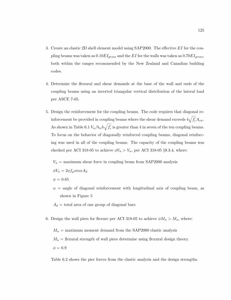
125
3. Create an elastic 2D shell element model using SAP2000. The effective EI for the cou-
pling beams was taken as 0.10EIgross and the EI for the walls was taken as 0.70EIgross,
both within the ranges recommended by the New Zealand and Canadian building
codes.
4. Determine the flexural and shear demands at the base of the wall and ends of the
coupling beams using an inverted triangular vertical distribution of the lateral load
per ASCE 7-05.
5. Design the reinforcement for the coupling beams. The code requires that diagonal re-
inforcement be provided in coupling beams where the shear demand exceeds 4√
f ′cAcw.
As shown in Table 6.1 Vu/bwh√
f ′c is greater than 4 in seven of the ten coupling beams.
To focus on the behavior of diagonally reinforced coupling beams, diagonal reinforc-
ing was used in all of the coupling beams. The capacity of the coupling beams was
checked per ACI 318-05 to achieve φVn > Vu, per ACI 318-05 §9.3.4, where:
Vu = maximum shear force in coupling beam from SAP2000 analysis
φVn = 2φfysinαAd
φ = 0.85
α = angle of diagonal reinforcement with longitudinal axis of coupling beam, as
shown in Figure 5
Ad = total area of one group of diagonal bars
6. Design the wall piers for flexure per ACI 318-05 to achieve φMn > Mu, where:
Mu = maximum moment demand from the SAP2000 elastic analysis
Mn = flexural strength of wall piers determine using flexural design theory.
φ = 0.9
Table 6.2 shows the pier forces from the elastic analysis and the design strengths.

126
Figure 6.3: Geometry of coupling beam diagonal bars (ICC 2007)
Table 6.1: Coupling beam forces and diagonal reinforcement
Level Vu Vu/Ag
√f ′
c Diagonal Ad ρd θ φVn Vu/φVn
(kips) (in) Bars (in2) (degrees) (kips)
10th 19.3 2.8 4-#4 0.8 0.83% 31.4 42 0.45
9th 24.1 3.6 4-#4 0.8 0.83% 31.4 42 0.57
8th 28.4 4.2 4-#4 0.8 0.83% 31.4 42 0.67
7th 32.9 4.8 4-#4 0.8 0.83% 31.4 42 0.77
6th 36.8 5.4 4-#4 0.8 0.83% 31.4 42 0.87
5th 39.6 5.8 4-#4 0.8 0.83% 31.4 42 0.93
4th 40.5 6.0 4-#4 0.8 0.83% 31.4 42 0.95
3rd 38.5 5.7 4-#4 0.8 0.83% 31.4 42 0.91
2nd 32.3 4.8 4-#4 0.8 0.83% 31.4 42 0.76
1st 19.6 2.9 4-#4 0.8 0.83% 31.4 42 0.46

127
Table 6.2: Calculation of factored axial forces and moments on wall piers
Level P ier Ag PD∗ PE Pumin Pumax Mu φMn Mu/φMn
(in2) (k) (k) (k) (k) (k − ft) (kips)
1st A 288 144 -311.9 -206.3 -115.1 501.0 163 3.07
1st B 288 144 311.9 417.5 508.7 501.0 904 0.55
Sum 1002.0 1067 0.94**
*(Assumed 0.1Agf′c)
**Total φMn > Mu, moment redistribution assumed
6.5 Recommended Plastic Design
As previously mentioned, the the 2006 IBC Seismic Design Manual recommends that a
plastic analysis be completed. The following steps detail the recommended plastic analysis
process and subsequent redesign of the wall piers.
1. Assume a behavior mechanism with plastic hinging at the base of the wall piers and
at each end of all the coupling beams as shown in Figure 6.1.
2. Determine the probable flexural strength, Mpr, of the coupling beams and piers. The
IBC example ignores the effect of axial loads on the wall piers due to seismic forces;
making the assumption that the increase in moment strength of the compression
pier and the decrease in moment strength of the tension pier will offset one another.
While in some cases this may be true, it is not always correct. In the plastic analysis
of the coupled wall for this study, the effect of axial loads due to seismic forces was
significant and was therefore included in the determination of Mpr. For the wall piers
Mpr was determined based on a moment curvature analysis of the pier section using
1.25fy and included the axial force due to gravity and seismic loads. For the coupling
beams Mpr was calculated as 1.25Vnln/2, assuming 1.25fy and only accounting for
the contribution from the diagonal reinforcement. This method ignores the effect of

128
additional longitudinal reinforcement that may be present in the beam to support the
stirrups and/or to provide skin reinforcement, however it is consistent with method
used to initially design the coupling beam.
3. Evaluate the plastic mechanism using internal vs. external work to determine the
plastic shear demand at the base of the wall.
The external work is calculated as the sum of the story displacement, δi, times the
story force, fxi as shown in Table 6.3. Plastic story displacements increase linearly
from the base to the top of the wall with he magnitude of δroof set to 2% at the roof.
The magnitude of the story displacements is arbitrary and will not change the output.
The story forces come from the code specified vertical distribution.
The internal work is calculated as the sum of the probable moment strength, Mpr,
times the plastic rotation angle, θ, for the coupling beams and the base wall piers
as shown in Table 6.4. The plastic rotation angle of the wall piers equals the roof
displacement divided by the roof height above the midpoint of the plastic hinge. The
plastic hinge length of the piers is assumed to be the wall length over two, lp = lw/2,
in this case 2ft. The plastic rotation angle of the coupling beams is calculated as
follows:
θcb = θlcln
where:
ln = the clear length of the coupling beams
lc = the distance between centroids of the wall piers
Assuming Mpr of the coupling beams equals 1.25Vnln/2, the internal work for each
coupling beam (counting both ends), can be calculated as θ1.25Vnlc.
Equating the internal work with the external work provides the base shear, or the
plastic shear demand. The calculations have are shown for the method of ignoring

129
Table 6.3: Plastic mechanism calculations - External Work
External WorkLevel hi hi − lp/2 δi fxi fxi/V Work/V
(ft) (ft) (ft) (k) (ft)10th 40 39 0.80 22.3 0.22 0.189th 36 35 0.72 15.5 0.16 0.118th 32 31 0.64 13.8 0.14 0.097th 28 27 0.55 12.1 0.12 0.076th 24 23 0.47 10.4 0.10 0.055th 20 19 0.39 8.6 0.09 0.034th 16 15 0.31 6.9 0.07 0.023rd 12 11 0.23 5.2 0.05 0.012nd 8 7 0.14 3.5 0.04 0.011st 4 3 0.06 1.7 0.02 0.00Sum 210 100 1.00 0.57
earthquake axial and including it. In this case, including the earthquake axial forces
resulted in a base shear of 191.0k, approximately 5% less than if it had been ignored.
4. Compare the plastic shear demand with the nominal shear strength, φVn, and adjust
the shear reinforcement to ensure flexural behavior in the wall. In this case, the
plastic shear demand was 190% of the initial shear demand used to design the wall.
The horizontal reinforcement in the first floor piers had to be doubled to ρ = 0.54%
in order to meet the increased shear demand.
The plastic analysis and design method resulted in an increase amount of shear rein-
forcement in the wall piers in he first level only, all other wall reinforcement remains per
the strength design. The final reinforcement layout shown in Figure 6.4.
6.6 Coupling Beam Reinforcement Details
The coupling beam confinement reinforcing was designed using two different approaches, the
current ACI 318 requirements and the proposed method from ACI Committee 318H-CH047.
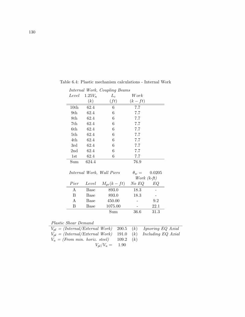
130
Table 6.4: Plastic mechanism calculations - Internal Work
Internal Work, Coupling BeamsLevel 1.25Vn Lc Work
(k) (ft) (k − ft)10th 62.4 6 7.79th 62.4 6 7.78th 62.4 6 7.77th 62.4 6 7.76th 62.4 6 7.75th 62.4 6 7.74th 62.4 6 7.73rd 62.4 6 7.72nd 62.4 6 7.71st 62.4 6 7.7Sum 624.4 76.9
Internal Work, Wall Piers θw = 0.0205Work (k-ft)
Pier Level Mpr(k − ft) No EQ EQA Base 893.0 18.3 -B Base 893.0 18.3 -A Base 450.00 - 9.2B Base 1075.00 - 22.1
Sum 36.6 31.3
Plastic Shear DemandVpl = (Internal/External Work) 200.5 (k) Ignoring EQ AxialVpl = (Internal/External Work) 191.0 (k) Including EQ AxialVu = (From min. horiz. steel) 109.2 (k)
Vpl/Vu = 1.90

131
The current ACI 318-05 code requires that each group of diagonally place bars be con-
fined per §21.4.4.1 through §21.4.4.3. Following these sections results in #2 ties at 2” O.C.
along the diagonal bars and #2 ties at 6” O.C. around the entire beam section.
The alternative design procedure of proposal 318H-CH047 allows for the entire coupling
beam section to be confined instead of providing confinement around each diagonal bar
group. Following this design method results in #2 ties at 1 1/2” O.C. around the entire
beam section. Additional cross ties are required to meet the minimum cross sectional
reinforcement area, Ash, and to satisfy the 8 inch spacing limit for cross-ties.
The two confinement options are shown in Figure 6.5 for the third scale coupling beam.
6.7 Coupled Wall Model Variations
A finite element model of the full ten-story coupled shear wall was created in VecTor2 at
one-third scale. Three variations of the wall were modeled, each with different coupling
beam reinforcement. The wall was modeled with coupling beams CBR-ACI, CBR-318H-F,
and CBR-318H-FR. A brief description of the coupling beams is presented here.
CBR-ACI This coupling beam is designed to meet the current ACI 318-05 code require-
ments. It contains diagonal reinforcing bars that are have confinement reinforcement
around each group of diagonal bars.
CBR-318H-F This coupling beam was detailed per ACI 318H-CH047 which will be pub-
lished in the 2008 version of the ACI code. It has the same diagonal reinforcing bars
as CBR-ACI, and thus the same design strength. However, in this design, confining
reinforcement is placed around the entire beam rather than just around he diagonal
bar groups.
CBR-318H-FR This coupling beam is designed to have a flexure/shear strength that
is 25% of CBR-318-HF. his coupling beam design was included because analysis of
coupled wall CW-318HF with coupling beam CBR-318-HF indicated that the coupling

132
Figure 6.4: Coupled Wall Reinforcement from Plastic Design

133
Figure 6.5: Coupling Beam Details
beams were not yielding and the assumed plastic mechanism was not being developed.
The amount of diagonal reinforcement in CBR-318H-FR was reduced from that in
CBR-318HF so that coupling beams would yield when the design level base shear,
Vn, was applied. The 75% reduction in strength was done by determining the tensile
stress demand in the diagonal bars of CW-318HF at the design level base shear and
then reducing the area of steel so that resulting force would be the same but the bars
would be at the yield stress level.
The three coupled wall models were identified as CW-ACI (includes coupling beam CBR-
ACI), CW-318HF (includes coupling beam CBR-318H-F), CW-318HFR (includes coupling
beam CBR-318H-FR). Details of the coupling beam designs and their expected performance
is presented in Chapter 5. Table 6.5 shows a summary of the reinforcement ratios for the
three coupled wall variations.
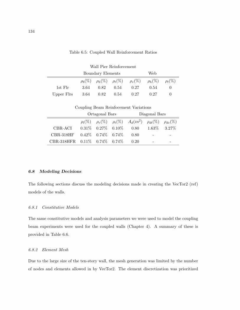
134
Table 6.5: Coupled Wall Reinforcement Ratios
Wall Pier Reinforcement
Boundary Elements Web
ρb(%) ρh(%) ρt(%) ρv(%) ρh(%) ρt(%)
1st Flr 3.64 0.82 0.54 0.27 0.54 0
Upper Flrs 3.64 0.82 0.54 0.27 0.27 0
Coupling Beam Reinfocement Variations
Ortagonal Bars Diagonal Bars
ρl(%) ρv(%) ρt(%) Ad(in2) ρdt(%) ρdv(%)
CBR-ACI 0.31% 0.27% 0.10% 0.80 1.63% 3.27%
CBR-318HF 0.42% 0.74% 0.74% 0.80 - -
CBR-318HFR 0.11% 0.74% 0.74% 0.20 - -
6.8 Modeling Decisions
The following sections discuss the modeling decisions made in creating the VecTor2 (ref)
models of the walls.
6.8.1 Constitutive Models
The same constitutive models and analysis parameters we were used to model the coupling
beam experiments were used for the coupled walls (Chapter 4). A summary of these is
provided in Table 6.6.
6.8.2 Element Mesh
Due to the large size of the ten-story wall, the mesh generation was limited by the number
of nodes and elements allowed in by VecTor2. The element discretization was prioritized
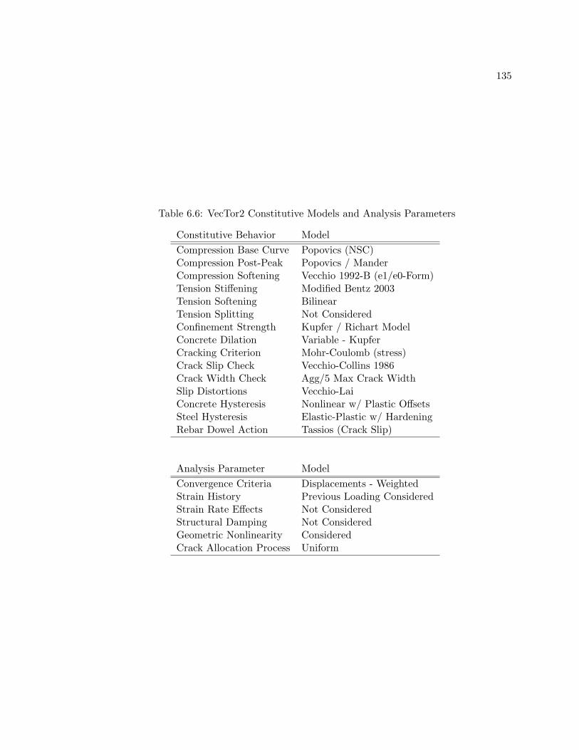
135
Table 6.6: VecTor2 Constitutive Models and Analysis Parameters
Constitutive Behavior ModelCompression Base Curve Popovics (NSC)Compression Post-Peak Popovics / ManderCompression Softening Vecchio 1992-B (e1/e0-Form)Tension Stiffening Modified Bentz 2003Tension Softening BilinearTension Splitting Not ConsideredConfinement Strength Kupfer / Richart ModelConcrete Dilation Variable - KupferCracking Criterion Mohr-Coulomb (stress)Crack Slip Check Vecchio-Collins 1986Crack Width Check Agg/5 Max Crack WidthSlip Distortions Vecchio-LaiConcrete Hysteresis Nonlinear w/ Plastic OffsetsSteel Hysteresis Elastic-Plastic w/ HardeningRebar Dowel Action Tassios (Crack Slip)
Analysis Parameter ModelConvergence Criteria Displacements - WeightedStrain History Previous Loading ConsideredStrain Rate Effects Not ConsideredStructural Damping Not ConsideredGeometric Nonlinearity ConsideredCrack Allocation Process Uniform

136
Figure 6.6: CW-ACI Coupled Wall Mesh

137
Figure 6.7: CW-318HF and CW-318HFR Coupled Wall Mesh

138
to allow for a finer mesh in the coupling beams and the boundary elements of the wall
piers, where more deformation and damage are expected, and a larger mesh size in the
web zone of the wall piers. The boundary zones and the web zone were each divided into
four elements. The coupling beams were divided into nine elements vertically and thirteen
elements longitudinally.
The mesh was generated using a grid of rectilinear elements and with the insertion of
triangular elements at transition between zones and along the diagonal truss bar elements.
Model CW-ACI is shown in its entirety with a detail of a single coupling beam in Figure 6.6.
The mesh for CW-318HF and CW-318HFR are the same and is shown in Figure 6.7.
6.8.3 Reinforcement Model
The diagonal reinforcing bars of each coupling beam were grouped together and modeled
with a discrete truss-bar element. The remaining reinforcement in the coupling beams
(longitudinal, vertical, and out-of-plane) and all reinforcement in the wall piers was modeled
with smeared reinforcement.
6.8.4 Boundary Conditions
The wall was designed assuming a fixed base, as is commonly done in engineering design
offices. To model this in VecTor2, all nodes along the bottom of the wall were fixed against
translation in both directions.
6.8.5 Loading Parameters
Two approaches were considered to control the analyses and apply lateral load to the wall.
The coupled wall was first modeled using displacement control and the assumption of a linear
deformed shape for the wall. However, this approach was abandoned when it was determined
that the story force distribution due to the assumed deformed shapes did not match those
expected due to earthquake loading. Details of the displacement control analysis and are
presented in section 6.10. Ultimately, the coupled walls were modeled using load control with

139
three different lateral load distributions. Due to the limitations in the VecTor2 software,
specifically the inability to maintain constant load pattern while increasing a second load
pattern, gravity load was not applied to the walls. Details of the loading parameters are
shown below.
Displacement Control
Two displaced shapes were considered; the displaced shape from the elastic SAP2000 model
and the displaced shape resulting from the assumed plastic mechanism used in the wall
design process. The elastic displaced shape was taken as an average of the displaced shapes
resulting from the uniform load pattern and the inverted triangular load pattern. The
resulting elastic displaced shape resembles that of a cantilevered beam with higher curvature
near the base of the wall and a near linear shape above the third floor. The plastic displaced
shape is purely a function of the assumed plastic hinges at the base of the wall and at the
ends of all the coupling beams and results in a linearly increasing displacement up the height
of the wall.
The two displaced shapes have been arbitrarily scaled to 10 at the top of the wall and
are shown in Table 6.7 and Figure 6.8 along with the uniform and triangular shapes.
Load Control
Three different lateral load distributions were considered; inverted triangular, uniform, and
uniform up to a height of 0.6Hwall to produce an effective height for the lateral load of
0.3Hwall. These load distributions are discussed in detail below:
• The Inverted Triangular lateral load distribution was defined using ASCE7-05, which
is the basis for the International Code Council 2007 design guidelines. Each story is
assumed to have the same mass. A “-T” is appended to the model name to indicate
this load distribution.
• Uniform lateral load distribution. Here the same load is applied to each story. A “-U”

140
Table 6.7: Coupled Wall Displaced Shapes
Scaled Displacement LevelLevel Plastic Unif. Tri. Elastic10 10.00 10.00 10.00 10.009 9.00 8.95 8.86 8.888 8.00 7.87 7.70 7.767 7.00 6.75 6.50 6.646 6.00 5.58 5.29 5.535 5.00 4.40 4.08 4.414 4.00 3.23 2.93 3.293 3.00 2.12 1.87 2.172 2.00 1.14 0.97 1.051 1.00 0.38 0.31 0.350 0.00 0.00 0.00 0.00
0 1 2 3 4 5 6 7 8 9 100
1
2
3
4
5
6
7
8
9
10
Leve
l
Displacement
Coupled Wall SpecimenDisplaced Shape
Assumed PlasticUniform Load SAP2000Tri. Load SAP2000Elastic
Figure 6.8: Coupled Wall Applied Displaced Shapes

141
is appended to the model name to indicate this load distribution.
• 0.3H Effective Height. This vertical distribution is designed to set the effective shear
height to 0.3 times the height of the wall. The same load is applied to the bottom
six floors of the wall. A “-3H” is appended to the model name to indicate this load
distribution.
For all of the load distributions, the load at each floor level was applied as four point
load distributed across the wall. The total load was increased monotonically until the
model became numerically unstable. Because the load, rather than the lateral displacement,
increased with each step in the analysis strength degradation of the wall could not be
simulated.
6.8.6 Summary of Coupled Wall Model Variations
With the multiple coupled wall models, control methods, and lateral load variations a matrix
of fifteen coupled wall models was necessary. The model name and a short summary of the
model characteristics are shown in Table 6.8.

142
Table 6.8: Coupled Wall Model List
Model Coupling Beam Analysis Method Load/Disp. Distribution
CW-ACI-T CBR-ACI Load Control Inv. Triangular
CW-ACI-U CBR-ACI Load Control Uniform
CW-ACI-3H CBR-ACI Load Control 0.3H Eff. Height
CW-318HF-T CBR-318H-F Load Control Inv. Triangular
CW-318HF-U CBR-318H-F Load Control Uniform
CW-318HF-3H CBR-318H-F Load Control 0.3H Eff. Height
CW-318HFR-T CBR-318H-FR Load Control Inv. Triangular
CW-318HFR-U CBR-318H-FR Load Control Uniform
CW-318HFR-3H CBR-318H-FR Load Control 0.3H Eff. Height
CW-ACI-PL CBR-ACI Disp. Control Plastic
CW-ACI-EL CBR-ACI Disp. Control Elastic
CW-318HF-PL CBR-318H-F Disp. Control Plastic
CW-318HF-EL CBR-318H-F Disp. Control Elastic
CW-318HFR-PL CBR-318H-F Disp. Control Plastic
CW-318HFR-EL CBR-318H-F Disp. Control Elastic
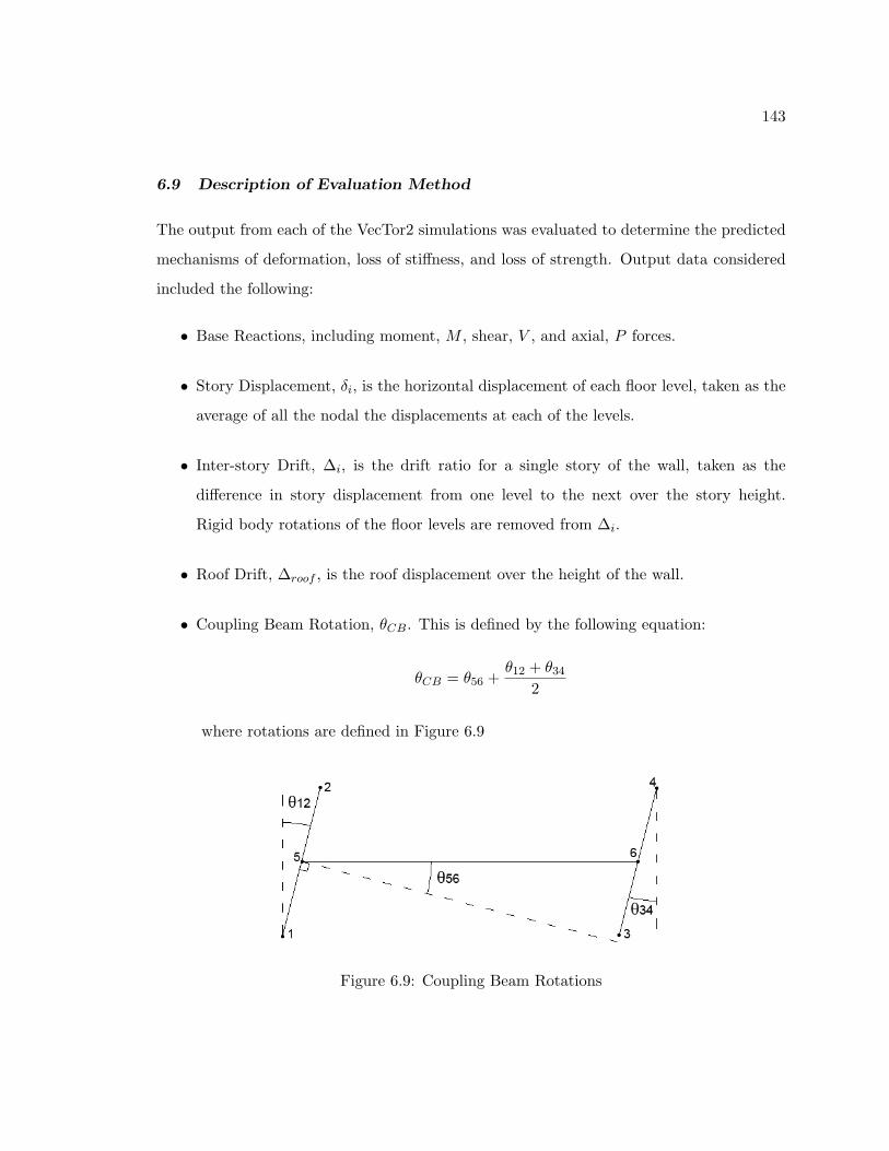
143
6.9 Description of Evaluation Method
The output from each of the VecTor2 simulations was evaluated to determine the predicted
mechanisms of deformation, loss of stiffness, and loss of strength. Output data considered
included the following:
• Base Reactions, including moment, M , shear, V , and axial, P forces.
• Story Displacement, δi, is the horizontal displacement of each floor level, taken as the
average of all the nodal the displacements at each of the levels.
• Inter-story Drift, ∆i, is the drift ratio for a single story of the wall, taken as the
difference in story displacement from one level to the next over the story height.
Rigid body rotations of the floor levels are removed from ∆i.
• Roof Drift, ∆roof , is the roof displacement over the height of the wall.
• Coupling Beam Rotation, θCB. This is defined by the following equation:
θCB = θ56 +θ12 + θ34
2
where rotations are defined in Figure 6.9
Figure 6.9: Coupling Beam Rotations

144
• Coupling Beam Displacement, δ, is calculated assuming small rotations and ignoring
axial elongation of the beam as:
δ = θL
where θCB is defined in Eqn. 6.9 and L is the length of the coupling beam.
• Coupling Beam Drift, ∆, is the coupling beam displacement over the its length, ac-
cording to Eqn. 6.9 ∆ = θCB.
• Degree of Coupling, DOC, is a measure of the percentage of the overturning moment
due to the base moment in the wall piers versus the percentage due to the wall axial
load, which results from the shear forces in the coupling beams (Harries 2001), defined
as:
DOC =TL
Mw(6.1)
where,
T = axial load in walls due to shears in coupling beams;
L = distance between the centroids of the wall piers; and,
Mw = total overturning moment in the base of the wall.
Additionally, the displaced shape, predicted plastic mechanism, crack patterns and failure
modes are discussed.
6.10 Displacement Control Results
The VecTor2 simulations were first attempted using an applied displacement approach.
The applied displacement was intended to simulate the displaced shape assumed during
the plastic design procedure. Due to the limitations of VecTor2, when using an applied
displacement, only the magnitude of the displacements can be incremented. There is no
capability to modify the displaced shape over the course of the simulation. This, of course,

145
0 20 40 60 80 100 120 1401
2
3
4
5
6
7
8
9
10
Leve
l
Displacement
Coupled Wall ModelsStory Force
VecTor2 PlasticUniform Load Dist.Tri. Load Dist.
Figure 6.10: Coupled Wall Story Force
does not represent the true displacement history of a coupled wall. The displaced shape of
the coupled wall will change with the magnitude and distribution of the applied load, with
the level of yielding and plastic deformation within the wall. The displaced shape could
approach the assumed plastic displaced shape if full plastic hinging is reached in the wall
piers and coupling beams.
Figure 6.10 shows the distribution of story shears under the assumed plastic displaced
shape compared to the story forces resulting from a uniform lateral force distribution and
the inverted triangular load distribution that was used during the design. The plot shows
that nearly all of the base shear in the plastic displaced shape model is developed over the
first story, indicating that the coupled wall is not behaving as expected.
The approach of applying a displacement to the wall proved to be inappropriate for sim-
ulating the response of the coupled wall and was ultimately abandoned in favor of following
the load control approach. To accurately simulate the behavior of a coupled wall during a

146
0 0.1 0.2 0.3 0.4 0.5 0.6 0.7 0.8 0.9 10
50
100
150
200
250
300
Bas
e S
hear
(K
ip)
Roof Drift (%)
Vu Plastic
CW−ACI−ELCW−318HF−ELCW−318HFR−EL
Figure 6.11: Coupled Wall Response with Applied Elastic Displacement
pushover analysis, the displaced shape cannot remain fixed, it must remain free to adapt to
the changing behavior of the coupled wall. The base shear vs. roof drift histories are shown
in Figures 6.11 and 6.12 for information only.
6.11 Load Control Results
6.11.1 Deformed Shape and Crack Patterns
The following section discusses the deformed shapes of the walls at the point of first yield
and at the maximum predicted base shear. The roof displacement and drift are noted on
each figure. The displacements have been magnified 20 times in order to make the curvature
and displacement patterns more visible. The crack directions for each shell element are show
with the red lines. A thin red line indicates a crack that is less than 0.04 in (1 mm) and a
thick red line indicates a crack larger than .08 in (2 mm).
The deformed shape and crack patterns are shown for all the coupled wall models.

147
0 0.1 0.2 0.3 0.4 0.5 0.6 0.7 0.8 0.9 10
50
100
150
200
250
300
Bas
e S
hear
(K
ip)
Roof Drift (%)
Vu Plastic
CW−ACI−PLCW−318HF−PLCW−318HFR−PL
Figure 6.12: Coupled Wall Response with Applied Plastic Displacement
Figures 6.13, 6.14, and 6.15 are grouped by coupled wall model and show the effects of the
lateral load distribution on at the maximum predicted base shear. Figures 6.16 to 6.21 are
grouped by lateral load distribution and show the effects of the changes in the coupling
beam reinforcement at the first yield point and at the maximum predicted base shear.
These figures show that there is a nominal difference in displaced shape and crack pat-
terns between the reference model, CW-ACI, and the full confinement model, CW-318HF.
Both models have the same concentration of plastic deformation and cracking at the base of
the wall piers with little to no deformation in the coupling beams. On the other hand, the
reduced coupling beam strength model, CW-318HFR, has a dramatically different displaced
shape with plastic deformation and cracking distributed over the ends of all of the coupling
beams and at the base of the wall piers.

148
Figure 6.13: CW-ACI Displacement Comparisson

149
Figure 6.14: CW-318HF Displacement Comparisson

150
Figure 6.15: CW-318HFR Displacement Comparison

151
Figure 6.16: Displacement Comparison at First Yield - Inverted Triangular Load
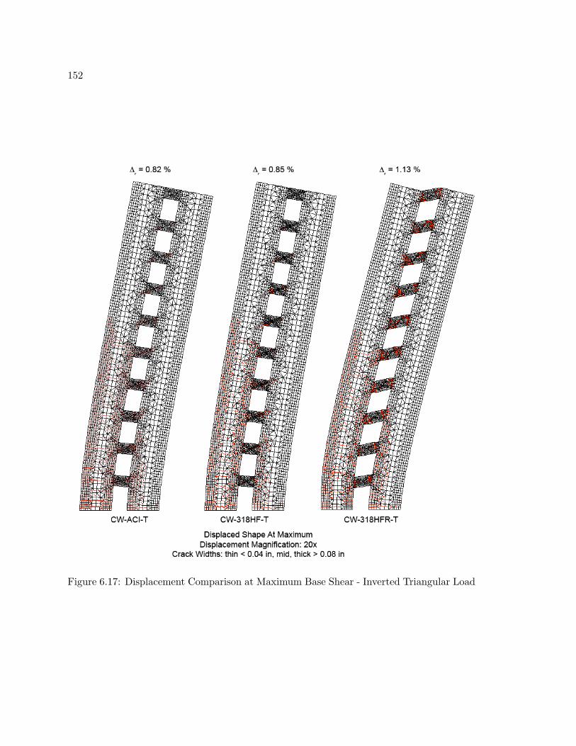
152
Figure 6.17: Displacement Comparison at Maximum Base Shear - Inverted Triangular Load
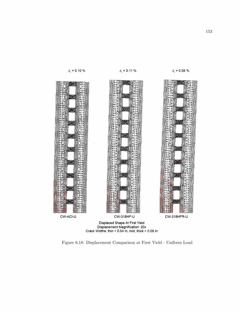
153
Figure 6.18: Displacement Comparison at First Yield - Uniform Load

154
Figure 6.19: Displacement Comparison at Maximum Base Shear - Uniform Load

155
Figure 6.20: Displacement Comparison at First Yield - 0.3H Effective Height Load

156
Figure 6.21: Displacement Comparison at Maximum Base Shear - 0.3H Effective HeightLoad
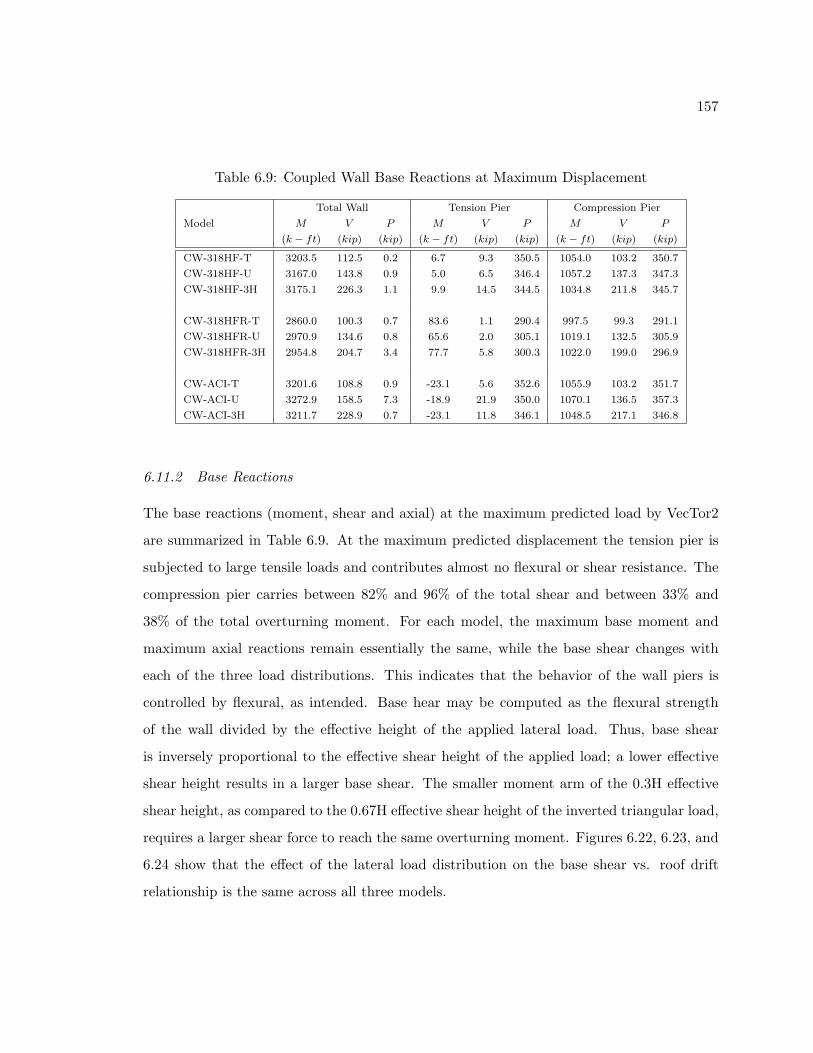
157
Table 6.9: Coupled Wall Base Reactions at Maximum Displacement
Total Wall Tension Pier Compression Pier
Model M V P M V P M V P
(k − ft) (kip) (kip) (k − ft) (kip) (kip) (k − ft) (kip) (kip)
CW-318HF-T 3203.5 112.5 0.2 6.7 9.3 350.5 1054.0 103.2 350.7
CW-318HF-U 3167.0 143.8 0.9 5.0 6.5 346.4 1057.2 137.3 347.3
CW-318HF-3H 3175.1 226.3 1.1 9.9 14.5 344.5 1034.8 211.8 345.7
CW-318HFR-T 2860.0 100.3 0.7 83.6 1.1 290.4 997.5 99.3 291.1
CW-318HFR-U 2970.9 134.6 0.8 65.6 2.0 305.1 1019.1 132.5 305.9
CW-318HFR-3H 2954.8 204.7 3.4 77.7 5.8 300.3 1022.0 199.0 296.9
CW-ACI-T 3201.6 108.8 0.9 -23.1 5.6 352.6 1055.9 103.2 351.7
CW-ACI-U 3272.9 158.5 7.3 -18.9 21.9 350.0 1070.1 136.5 357.3
CW-ACI-3H 3211.7 228.9 0.7 -23.1 11.8 346.1 1048.5 217.1 346.8
6.11.2 Base Reactions
The base reactions (moment, shear and axial) at the maximum predicted load by VecTor2
are summarized in Table 6.9. At the maximum predicted displacement the tension pier is
subjected to large tensile loads and contributes almost no flexural or shear resistance. The
compression pier carries between 82% and 96% of the total shear and between 33% and
38% of the total overturning moment. For each model, the maximum base moment and
maximum axial reactions remain essentially the same, while the base shear changes with
each of the three load distributions. This indicates that the behavior of the wall piers is
controlled by flexural, as intended. Base hear may be computed as the flexural strength
of the wall divided by the effective height of the applied lateral load. Thus, base shear
is inversely proportional to the effective shear height of the applied load; a lower effective
shear height results in a larger base shear. The smaller moment arm of the 0.3H effective
shear height, as compared to the 0.67H effective shear height of the inverted triangular load,
requires a larger shear force to reach the same overturning moment. Figures 6.22, 6.23, and
6.24 show that the effect of the lateral load distribution on the base shear vs. roof drift
relationship is the same across all three models.

158
0 0.1 0.2 0.3 0.4 0.5 0.6 0.7 0.8 0.9 10
50
100
150
200
250
Bas
e S
hear
(K
ip)
Roof Drift (%)
Vu Design
CW−318HF−TCW−318HF−UCW−318HF−3H
Figure 6.22: CW-318HF - Effect of Load Distribution
0 0.2 0.4 0.6 0.8 1 1.20
50
100
150
200
250
Bas
e S
hear
(K
ip)
Roof Drift (%)
Vu Design
CW−318HFR−TCW−318HFR−UCW−318HFR−3H
Figure 6.23: CW-318HFR - Effect of Load Distribution

159
0 0.1 0.2 0.3 0.4 0.5 0.6 0.7 0.8 0.9 10
50
100
150
200
250
Bas
e S
hear
(K
ip)
Roof Drift (%)
Vu Design
CW−ACI−TCW−ACI−UCW−ACI−3H
Figure 6.24: CW-ACI - Effect of Load Distribution

160
Table 6.10: Coupled Wall Degree of Coupling
Model T Mw TL DOC DOC
(kip) (k − ft) (k − ft) V ecTor2 Theoretical
CW-318HF-T 350.6 3203.5 2103.6 0.66 0.71
CW-318HF-U 346.9 3167.0 2081.1 0.66 0.71
CW-318HF-3H 345.1 3175.1 2070.6 0.65 0.71
CW-318HFR-T 290.8 2860.0 1744.5 0.61 0.38
CW-318HFR-U 305.5 2970.9 1833.0 0.62 0.38
CW-318HFR-3H 298.6 2954.8 1791.6 0.61 0.38
CW-ACI-T 352.2 3201.6 2112.9 0.66 0.71
CW-ACI-U 353.7 3272.9 2121.9 0.65 0.71
CW-ACI-3H 346.5 3211.7 2078.7 0.65 0.71
6.11.3 Degree of Coupling
The degree of coupling (DOC) calculated using the internal forces at the maximum predicted
load is summarized in Table 6.10. The theoretical degree of coupling for walls CW-ACI and
CW-318HF, based on the expected strengths (Vpr,Mpr), is 0.71. The lower value computed
using results from the VecTor2 analysis shows the coupling beams are carrying less of the
resistance than assumed during the design. This is due to the fact that only a few, rather
than all, of the coupling beams actually yielded.
To obtain the desired behavior mode, with yielding at the base of the wall piers and at the
ends of all of the coupling beams, Harries (2001) recommends that the degree of coupling
should not exceed 0.50. This recommendation is based on a comprehensive analysis of
approximately thirty coupled wall models completed by nine researchers over the last thirty
years. His study found that a high degree of coupling will cause a coupled wall to behave

161
Table 6.11: Coupled Wall Roof Drift
Model First Yield Max Predicted Disp.
Vy δy ∆y Vu δu ∆u
(kip) (in) (%) (kip) (in) (%)
CW-318HF-T 56.9 0.72 0.15% 112.5 4.09 0.85%
CW-318HF-U 67.4 0.56 0.12% 143.8 4.54 0.95%
CW-318HF-3H 126.8 0.53 0.11% 226.3 2.36 0.49%
CW-318HFR-T 51.9 0.62 0.11% 100.3 5.44 1.13%
CW-318HFR-U 60.7 0.44 0.09% 134.6 5.01 1.04%
CW-318HFR-3H 99.8 0.39 0.08% 209.6 4.40 0.92%
CW-ACI-T 51.9 0.57 0.12% 108.8 3.94 0.82%
CW-ACI-U 74.1 0.62 0.13% 158.5 4.17 0.87%
CW-ACI-3H 118.7 0.48 0.10% 228.9 3.24 0.67%
similar to a planar wall where the energy dissipation and plastic deformation is concentrated
at the base of the wall.
6.11.4 Displacement and Drift at Yield and Maximum
The roof drift and base shear at first yield of the wall piers and at the maximum predicted
base shear are summarized in Table 6.11. Models CW-ACI and CW-318HF have very similar
roof drift ratios at both points of reference. This similarity is expected given that the two
coupled wall models have the same design strength for the piers and coupling beams. Model
CW-318HFR, while reaching a lower base shear strength, has the highest roof drift ratios
of all the models.
Brown (2006) reviewed experimental data for planar wall tests and found that the mean
drift at first yield in the walls was 0.47% and the mean drift at the ultimate or failure point

162
0 0.2 0.4 0.6 0.8 1 1.20
50
100
150
Bas
e S
hear
(K
ip)
Roof Drift (%)
Vu Design
CW−318HF−TCW−318HFR−TCW−ACI−T
Figure 6.25: Base Shear vs. Roof Drift - Triangular Load
was 1.92%. The coupled wall drift values predicted by VecTor2 are lower than these averages,
however this difference is likely due to the modeling limitations of the finite element analysis
within VecTor2 and not the limitations of the wall. Recall that in the coupling validation
study presented in Chapter 4, VecTor2 under-predicted the yield drift by an average of 11%
and under-predicted the ultimate drift by an average of 42%. If these averages are be applied
to the average coupled wall model drifts, the true yield drift would be approximately 13%.
Correspondingly, the true ultimate drifts would be 1.34% for CW-ACI and CW-318HF and
1.78% for CW-318HFR.
6.11.5 Base Shear vs. Drift Comparisons
Figures 6.25, 6.26, and 6.27 illustrate the effect of the reduced strength coupling beams on
the load-drift plots for coupled wall models under each of the three loading methods. Model
CW-318HFR on average has reaches an ultimate shear capacity that is 10% less than the
other two models, however maximum shear is reached at a drift that is 30% larger than for

163
0 0.2 0.4 0.6 0.8 1 1.20
20
40
60
80
100
120
140
160
180
200
Bas
e S
hear
(K
ip)
Roof Drift (%)
Vu Design
CW−318HF−UCW−318HFR−UCW−ACI−U
Figure 6.26: Base Shear vs. Roof Drift - Uniform Load
0 0.2 0.4 0.6 0.8 1 1.20
50
100
150
200
250
Bas
e S
hear
(K
ip)
Roof Drift (%)
Vu Design
CW−318HF−3HCW−318HFR−3HCW−ACI−3H
Figure 6.27: Base Shear vs. Roof Drift - 0.3H Effective Height Load
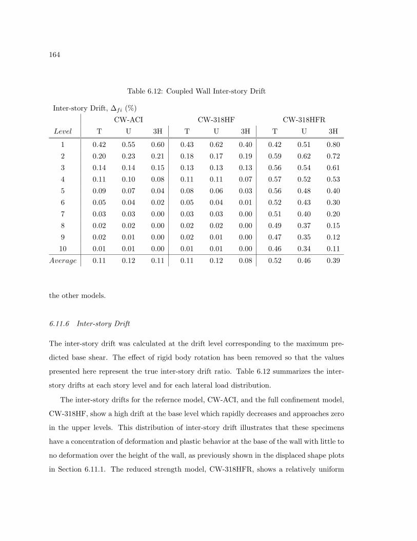
164
Table 6.12: Coupled Wall Inter-story Drift
Inter-story Drift, ∆fi (%)
CW-ACI CW-318HF CW-318HFR
Level T U 3H T U 3H T U 3H
1 0.42 0.55 0.60 0.43 0.62 0.40 0.42 0.51 0.80
2 0.20 0.23 0.21 0.18 0.17 0.19 0.59 0.62 0.72
3 0.14 0.14 0.15 0.13 0.13 0.13 0.56 0.54 0.61
4 0.11 0.10 0.08 0.11 0.11 0.07 0.57 0.52 0.53
5 0.09 0.07 0.04 0.08 0.06 0.03 0.56 0.48 0.40
6 0.05 0.04 0.02 0.05 0.04 0.01 0.52 0.43 0.30
7 0.03 0.03 0.00 0.03 0.03 0.00 0.51 0.40 0.20
8 0.02 0.02 0.00 0.02 0.02 0.00 0.49 0.37 0.15
9 0.02 0.01 0.00 0.02 0.01 0.00 0.47 0.35 0.12
10 0.01 0.01 0.00 0.01 0.01 0.00 0.46 0.34 0.11
Average 0.11 0.12 0.11 0.11 0.12 0.08 0.52 0.46 0.39
the other models.
6.11.6 Inter-story Drift
The inter-story drift was calculated at the drift level corresponding to the maximum pre-
dicted base shear. The effect of rigid body rotation has been removed so that the values
presented here represent the true inter-story drift ratio. Table 6.12 summarizes the inter-
story drifts at each story level and for each lateral load distribution.
The inter-story drifts for the refernce model, CW-ACI, and the full confinement model,
CW-318HF, show a high drift at the base level which rapidly decreases and approaches zero
in the upper levels. This distribution of inter-story drift illustrates that these specimens
have a concentration of deformation and plastic behavior at the base of the wall with little to
no deformation over the height of the wall, as previously shown in the displaced shape plots
in Section 6.11.1. The reduced strength model, CW-318HFR, shows a relatively uniform

165
Table 6.13: Coupling Beam Drift
Coupling Beam Drift, ∆CB (%)
CW-ACI CW-318HF CW-318HFR
Level T U 3H T U 3H T U 3H
1 0.03 0.05 0.16 0.03 0.04 0.15 1.11 1.30 2.04
2 0.09 0.14 0.25 0.09 0.12 0.21 2.00 2.12 2.65
3 0.16 0.18 0.23 0.10 0.13 0.17 2.31 2.25 2.56
4 0.12 0.13 0.17 0.09 0.10 0.13 2.46 2.22 2.25
5 0.10 0.11 0.10 0.08 0.10 0.08 2.51 2.13 1.82
6 0.10 0.09 0.05 0.08 0.08 0.04 2.47 2.02 1.36
7 0.08 0.07 0.02 0.07 0.06 0.01 2.42 1.89 0.95
8 0.06 0.04 0.01 0.05 0.04 0.00 2.35 1.79 0.70
9 0.04 0.03 0.00 0.04 0.03 0.00 2.29 1.71 0.58
10 0.02 0.01 0.00 0.02 0.01 0.00 2.11 1.55 0.46
Average 0.08 0.08 0.10 0.07 0.07 0.08 2.20 1.90 1.54
distribution of inter-story drift over the hight of the wall, indicating a uniform distribution
of deformation and plastic behavior.
6.11.7 Coupling Beam Rotation
The coupling beam drift can be compared to the drift predictions of the coupling beam
simulations presented in chapter 5. The coupling beam simulations predicted a yield drift
of 0.57% for CBR-ACI and CBR-318H-F. These are the same coupling beams as are present
in the coupled wall models, CW-ACI and CW-318HF. The maximum coupling beam drift
predicted in these two coupled walls was 0.25%, which is well below the drift demand at
the predicted yield point of the coupling beams. This further illustrates that plastic hinges
did not form at the ends of the coupling beams as assumed during the plastic analysis and
design.
The reduced strength model, CW-318HFR, shows coupling beam drifts ranging from

166
0.46% to 2.65% over the height of the wall. These drifts indicate that coupling beams were
subjected to sufficient drift demands to cause yielding and plastic hinging to occur in the
coupling beam ends.
6.11.8 Reinforcement Yield
In this section the base shear versus roof drift plots for each of the coupled wall models are
presented. The plots are annoted to show the locations of first yielding for the different
components within the wall. The locations and type of reinforcement where yielding was
observed include:
• first yield of longitudinal (vertical) reinforcement in the tension pier,
• first yield of of the horizontal reinforcement in a coupling beam,
• first yield of longitudinal (vertical) reinforcement in the compression pier,
• first yield of the diagonal reinforcement in a coupling beam,
• majority of coupling beam diagonal bars yielded, five or more coupling beams.
The results from the reference model, CW-ACI, and the full confinement model, CW-
318HF, predicted an early yielding of the longitudinal reinforcement in the tension pier,
followed by yielding of the horizontal reinforcement in the coupling beams and yielding
of the longitudinal reinforcement in the compression pier. The diagonal reinforcement in
the coupling beams did not yield when subjected to the uniform or the inverted triangular
lateral load distributions, however under the 0.3H effective height distribution yielding of
the diagonal reinforcement did occur near the maximum predicted base shear.
The results from the reduced strength model, CW-318HFR, predicted that yielding of
the longintudinal reinforcement in the tension pier and the diagonal reinforcement of the
coupling beams occured at similar drift levels. The majority of the coupling beams yielded
within 0.05% roof drift of the point when the first diagonal bar yielded.

167
0 0.1 0.2 0.3 0.4 0.5 0.6 0.7 0.8 0.90
20
40
60
80
100
120
Bas
e S
hear
(K
ip)
Roof Drift (%)
Coupled Wall CW−ACI−TInv. Triangular Load Distribution
1st yield in tension pier
1st yield in comp. pier
1st yield in horiz. C.B. bar
CW−ACI−T
Figure 6.28: CW-ACI-T Roof Drift vs. Base Shear Response
0 0.1 0.2 0.3 0.4 0.5 0.6 0.7 0.8 0.90
20
40
60
80
100
120
140
160
Bas
e S
hear
(K
ip)
Roof Drift (%)
Coupled Wall CW−ACI−UUniform Load Distribution
1st yield in tension pier
1st yield in comp. pier
1st yield in horiz. C.B. bar
CW−ACI−U
Figure 6.29: Coupled Wall ACI-U Roof Drift vs. Base Shear Response

168
0 0.1 0.2 0.3 0.4 0.5 0.6 0.70
50
100
150
200
250B
ase
She
ar (
Kip
)
Roof Drift (%)
Coupled Wall CW−ACI−3H0.3H Eff. Height Load Distribution
1st yield in tension pier
1st yield in comp. pier
1st yield in horiz. C.B. bar
1st yield in diag. bar
CW−ACI−3H
Figure 6.30: Coupled Wall ACI-3H Roof Drift vs. Base Shear Response
0 0.1 0.2 0.3 0.4 0.5 0.6 0.7 0.8 0.90
20
40
60
80
100
120
Bas
e S
hear
(K
ip)
Roof Drift (%)
Coupled Wall CW−318F−TInv. Triangular Load Distribution
1st yield in tension pier
1st yield in comp. pier
1st yield in horiz. C.B. bar
CW−318F−T
Figure 6.31: CW-318HF-T Roof Drift vs. Base Shear Response

169
0 0.1 0.2 0.3 0.4 0.5 0.6 0.7 0.80
50
100
150
Bas
e S
hear
(K
ip)
Roof Drift (%)
Coupled Wall CW−318F−UUniform Load Distribution
1st yield in tension pier
1st yield in comp. pier
1st yield in horiz. C.B. bar
CW−318F−U
Figure 6.32: CW-318HF-U Roof Drift vs. Base Shear Response
0 0.05 0.1 0.15 0.2 0.25 0.3 0.35 0.4 0.45 0.50
50
100
150
200
250
Bas
e S
hear
(K
ip)
Roof Drift (%)
Coupled Wall CW−318F−3H0.3H Eff. Height Load Distribution
1st yield in tension pier
1st yield in comp. pier
1st yield in horiz. C.B. bar
1st yield in diag. bar
CW−318F−3H
Figure 6.33: CW-318HF-3H Roof Drift vs. Base Shear Response

170
0 0.2 0.4 0.6 0.8 1 1.2 1.40
20
40
60
80
100
120B
ase
She
ar (
Kip
)
Roof Drift (%)
Coupled Wall CW−318FR−TInv. Triangular Load Distribution
1st yield in tension pier
1st yield in comp. pier
1st yield in horiz. C.B. bar
1st yield in diag. barmajority of diag. bar yield
CW−318FR−T
Figure 6.34: CW-318HFR-T Roof Drift vs. Base Shear Response
0 0.2 0.4 0.6 0.8 1 1.2 1.40
20
40
60
80
100
120
140
Bas
e S
hear
(K
ip)
Roof Drift (%)
Coupled Wall CW−318FR−UUniform Load Distribution
1st yield in tension pier, 1st yield in diag. bar
1st yield in comp. pier
1st yield in horiz. C.B. bar
majority of diag. bar yield
CW−318FR−U
Figure 6.35: CW-318HFR-U Roof Drift vs. Base Shear Response

171
0 0.1 0.2 0.3 0.4 0.5 0.6 0.7 0.8 0.9 10
50
100
150
200
250
Bas
e S
hear
(K
ip)
Roof Drift (%)
Coupled Wall CW−318FR−3H0.3H Eff. Height Load Distribution
1st yield in tension pier
1st yield in comp. pier
1st yield in horiz. C.B. bar
1st yield in diag. bar
majority of diag. bar yield
CW−318FR−3H
Figure 6.36: CW-318HFR-3H Roof Drift vs. Base Shear Response

172
6.12 Conclusions
Evaluation of the VecTor2 simulation of the coupled wall modes supports the following
observations and conclusions:
• VecTor2 should not be used to complete a displacement based pushover analysis where
the displaced shape of the model may change during the simulation.
• The effects of the lateral load distribution can be related to the effective shear height of
the applied load. A higher effective shear height (i.e. inverted triangular distribution)
will cause the coupled wall to develop a smaller base shear and will allow it to reach
a higher roof drift. Conversely, a lower effective shear height (i.e. 0.3H effective shear
height distribution) will cause the coupled wall to develop a higher base shear but will
cause it to fail at a smaller roof drift. These results were expected and add support
to the validity of the VecTor2 analysis software.
• The VecTor2 simulations shows that the “desired” plastic mechanism for a coupled
wall, as recommended by the International Code Council (2007), is unlikely to occur
in a coupled wall that is designed according to these recommendations. The coupling
beams are too strong in comparison to the wall piers; yielding of the wall reinforcement
and crushing failure at the toe of the wall occur before the coupling beams can be
subjected to sufficient drift demands to cause yielding. The maximum coupling beam
drift seen in the coupled wall models designed using the ICC recommendations was
0.21%, which is far below the 0.57% average yield drift predicted in Chapter 5.
• In order to achieve the desired plastic mechanism in the coupled wall, the shear and
moment strength of the coupling beams was reduced to 25% of the design strength.
This reduced strength was determined by balancing the area of steel in the diagonal
reinforcement with the tensile stress demand in those bars at the design level base
shear. The reduced strength of the coupling beams allowed the coupled wall to perform

173
as desired with plastic hinging at the base of the wall piers and at the ends of all the
coupling beams. Despite the much lower shear and flexural strength of the coupling
beams, the maximum base shear of the coupled wall was only reduced on average by
10%.

174
Chapter 7
SUMMARY AND CONCLUSIONS
7.1 Summary
A ten-story coupled shear wall specimen was designed using state of the art performance
based design methods with the intent to provide a wall that will behave in a ductile manner
under seismic loading. The coupled wall is designed to develop plastic hinges at the base of
the wall piers and at the ends of all the coupling beams. Nonlinear finite element models
were created and pushover simulations completed to predict the behavior of the wall. Mul-
tiple versions of the coupled wall with different coupling beam reinforcement were analyzed
to investigate the effect of coupling beam confinement reinforcement and coupling beam
strength on the behavior of the wall. The simulation results suggest that a coupled wall
designed per current design recommendations will not behave as intended. The coupling
beam strength must be greatly reduced in order to achieve the desired plastic mechanism
and behavior mode.
The effects of coupling beam confinement on diagonally reinforced coupling beams were
investigated. Coupling beams following the current code requirements, with confinement
around the diagonal bar groups, were compared to proposed alternative design methods
with full confinement of the entire beam section. Finite element simulations suggest that
the proposed full confinement methods can meet or exceed the current detailing methods.
Data from previous experimental studies of coupling beam behavior were used to validate
the nonlinear analysis software and modeling assumptions.
175
7.2 Conclusions
The results of this study support the following observations and conclusions about coupling
beam confinement effects and coupled shear wall behavior:
Coupling Beams
• The ACI 318H-CH047 proposed revision to increase the spacing requirements on the
confinement ties around the diagonally placed reinforcement will have a negligible
effect on the performance of the coupling beam, and is capable of meeting the design
intent of the current ACI 318-05 specifications.
• VecTor2 simulations of coupling beams designed to meet the alternative design meth-
ods of the ACI 318H-CH047 proposal suggests that the shear strength and drift ca-
pacity of diagonally reinforced coupling beams can be increased by providing full
confinement of the entire section.
Coupled Shear Walls
• The VecTor2 simulations shows that the “desired” plastic mechanism for a coupled
wall, as recommended by the International Code Council (2007), is unlikely to occur
in a coupled wall that is designed according to these recommendations. The coupling
beams are too strong in comparison to the wall piers; yielding of the wall reinforcement
and crushing failure at the toe of the wall occur before the coupling beams can be
subjected to sufficient drift demands to cause yielding. The maximum coupling beam
drift seen in the coupled wall models designed using the ICC recommendations was
0.21%, which is far below the 0.57% average yield drift predicted in Chapter 5.
• In order to achieve the desired plastic mechanism in the coupled wall, the shear and
moment strength of the coupling beams was reduced to 25% of the design strength.
The reduced strength of the coupling beams allowed the coupled wall to perform as
176
desired, with plastic hinging at the base of the wall piers and at the ends of the
coupling beams. Despite the lower shear and flexural strength of the coupling beams,
the maximum base shear of the coupled wall was only reduced on average by 10%.
7.3 Recommendations for Further Work
• Explore the effect of the coupling beam aspect ratio on the coupled wall performance.
It is possible that the “desired” plastic mechanism may be easier to achieve if the
coupling beam aspect ratio is larger.
• Find a way to model strength degradation portion of the coupled wall push-over curve.
It would be useful to understand what the displacement capacity of the coupled wall
system is after the maximum predicted base shear is reached.
• Complete the analysis of the coupled wall models under cyclic loading.
• Include the effects of gravity loads on the coupled wall model simulations.
• Develop a design methodology that can provide a coupled wall that will allow yielding
in the wall piers and at the ends of all the coupling beams.
• Develop a method to account for the over-strenth in coupling beams that are confined
with the full confinement method proposed in ACI 319H-CH047.

177
BIBLIOGRAPHY
ACI Committee 318 (2005). Building Code Requirements for Structural Concrete and
Commentary. Farmington Hills, Mich.: American Concrete Institute. 430 pp.
Bristowe, S. (2000). Seismic Response of Normal and High Strength Concrete Members.
Ph. D. thesis, McGill University, Montreal, Quebec, Canada. 244 pp.
Brown, P. (2006). Probabilistic earthquake damage prediction for reinforced concrete
building components. Master’s thesis, University of Washington, Seattle.
Canadian Standards Association (2004). CSA A23.3-04: Design of Concrete Structures.
CSA International. 240 pp.
Galano, L. and A. Vignoli (2000, November). Seismic behavior of short coupling beams
with different reinforcement layouts. ACI Structural Journal 97 (6), 876–885.
Harries, K. A. (2001, August). Ductility and Deformability of Coupling Beams in Rein-
forced Concrete Coupled Walls. Earthquake Spectra 17 (3), 457–478.
Harries, K. A., P. J. Fortney, B. M. Shahrooz, and P. J. Brienen (2005, November).
Practical Design of Diagonally Reinforced Concrete Coupling Beams - Critical Review
of ACI 318 Requirements. ACI Structural Journal 102 (6), 876–882.
Harries, K. A., B. Gong, and B. M. Shahrooz (2000, November). Behavior and Design
of Reinforced Concrete, Steel, and Steel-Concrete Coupling Beams. Earthquake Spec-
tra 16 (4), 775–799.
Harries, K. A., J. D. Moulton, and R. L. Clemson (2004, March). Parametric Study of
Coupled Wall Behavior - Implications for the Design of Coupling Beams. Journal of
Structural Engineering 130 (3), 480–488.
International Code Council (January 2007). 2006 IBC Structural/Seismic Design Manual,
Volume 3. ICC.
Kwan, A. K. H. and Z. Z. Zhao (2002a, August). Cyclic behavior of deep reinforced
concrete coupling beams. Structures & Buildings 152 (3), 283–293.

178
Kwan, A. K. H. and Z. Z. Zhao (2002b, February). Testing of coupling beams with
equal end rotations maintained and local joint deformations allowed. Structures &
Buildings 152 (1), 67–78.
MATLAB (2005). Version 7.1. The MathWorks. www.mathworks.com/.
New Zealand Standards Association (2006). NZS 3101 Parts 1 and 2: 2006 Concrete
Structures Standard. New Zealand Standards Association. 646 pp.
Oyen, P. (2006). Evaluation of analytical tools for determining the seismic response of
reinforced concrete shear walls. Master’s thesis, University of Washington, Seattle.
Paulay, T. (1971). Coupling beams of reinforced concrete shear walls. Journal of the
Structural Division, ASCE 97 (ST3), 843–862.
Paulay, T. and J. R. Binney (1974). Diagonally Reinforced Coupling Beams of Shear
Walls. ACI Special Publication 42 - Shear in Reinforced Concrete, 579–598.
Santhakumar, A. R. (1974). Ductility of Coupled Shear Walls. Ph. D. thesis, University
of Canterbury, New Zealand.
SAP2000 (2006). Version 9.2. Computers and Structures, Inc. www.csiberkeley.com/.
Shiu, K. N., A. E. Fiorato, G. B. Barney, and W. G. Corley (1978). Reversing load tests
of reinforced concrete coupling beams. Central American Conference on Earthquake
Engineering , 239–249.
Structural Engineering Institute (2006). Minimum Design Loads for Buildings And Other
Structures: ASCE/SEI 7-05 (ASCE Standard No. 7-05). Reston, Virginia: American
Society of Civil Engineers. 424 pp.
Tassios, T. P., M. Maretti, and A. Bezas (1996, November). On the behavior and ductility
of reinforced concrete coupling beams of shear walls. ACI Structural Journal 93 (6),
711–720.
Tegos, I. A. and G. G. Penelis (1988). Seismic resistance of short columns and coupling
beams reinforced with inclined bars. ACI Structural Journal 85 (1), 82–88.
Vecchio, F. J. (2000). Disturbed stress field model for reinforced concrete: Formulation.
Journal of Structural Engineering 126 (9), 1070–1077.

179
Vecchio, F. J. (2001). Disturbed stress field model for reinforced concrete: Implementa-
tion. Journal of Structural Engineering 127 (1), 12–20.
Vecchio, F. J. and M. P. Collins (1986). The modified compression-field theory for rein-
forced concrete elements subject to shear. Journal of the American Concrete Insti-
tute 83 (2), 258–268.
Vecchio, F. J. and P. S. Wong (2006). VecTor2 & FormWorks User’s Manual. Vector
Analysis Group, University of Toronto. 201 pp.
VecTor2 (2006). Version 2.3. Vector Analysis Group. www.civ.utoronto.ca/vector/.
Zhao, Z. Z., A. K. H. Kwan, and X. G. He (2004, January). Nonlinear finite element
analysis of deep reinforced concrete coupling beams. Engineering Structures 26 (1),
13–25.

180
Appendix A
EXPERIMENTAL COUPLING BEAM LOAD DISPLACEMENTPLOTS

181
0 10 20 30 40 50 600
50
100
150
200
250
300
She
ar (
KN
)
Displacement (mm)
Galano P01
ExperimentalVector − Smeared
Figure A.1: Galano P01 - Vector2 Force-Disp. Smeared Reinf.
Figure A.2: Galano - Experimental Force-Disp. Plot
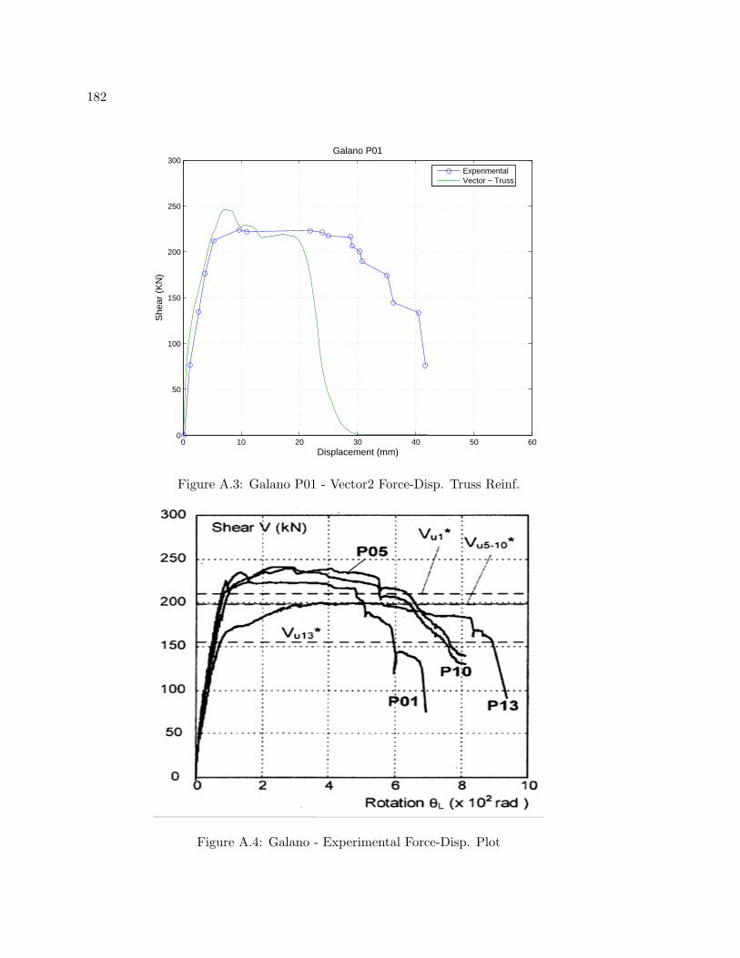
182
0 10 20 30 40 50 600
50
100
150
200
250
300S
hear
(K
N)
Displacement (mm)
Galano P01
ExperimentalVector − Truss
Figure A.3: Galano P01 - Vector2 Force-Disp. Truss Reinf.
Figure A.4: Galano - Experimental Force-Disp. Plot

183
−40 −30 −20 −10 0 10 20 30 40−300
−200
−100
0
100
200
300
She
ar (
KN
)
Displacement (mm)
Galano P02
ExperimentalVector − Smeared
Figure A.5: Galano P02 - Vector2 Force-Disp. Smeared Reinf.
Figure A.6: Galano P02 - Experimental Force-Disp. Plot

184
−40 −30 −20 −10 0 10 20 30 40−300
−200
−100
0
100
200
300S
hear
(K
N)
Displacement (mm)
Galano P02
ExperimentalVector − Truss
Figure A.7: Galano P02 - Vector2 Force-Disp. Truss Reinf.
Figure A.8: Galano P02 - Experimental Force-Disp. Plot
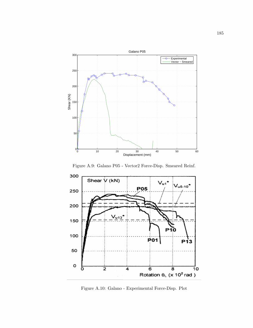
185
0 10 20 30 40 50 600
50
100
150
200
250
300
She
ar (
KN
)
Displacement (mm)
Galano P05
ExperimentalVector − Smeared
Figure A.9: Galano P05 - Vector2 Force-Disp. Smeared Reinf.
Figure A.10: Galano - Experimental Force-Disp. Plot

186
0 10 20 30 40 50 600
50
100
150
200
250
300S
hear
(K
N)
Displacement (mm)
Galano P05
ExperimentalVector − Truss
Figure A.11: Galano P05 - Vector2 Force-Disp. Truss Reinf.
Figure A.12: Galano - Experimental Force-Disp. Plot

187
−40 −30 −20 −10 0 10 20 30 40−300
−200
−100
0
100
200
300
She
ar (
KN
)
Displacement (mm)
Galano P07
ExperimentalVector − Smeared
Figure A.13: Galano P07 - Vector2 Force-Disp. Smeared Reinf.
Figure A.14: Galano P07 - Experimental Force-Disp. Plot

188
−40 −30 −20 −10 0 10 20 30 40−300
−200
−100
0
100
200
300S
hear
(K
N)
Displacement (mm)
Galano P07
ExperimentalVector − Truss
Figure A.15: Galano P07 - Vector2 Force-Disp. Truss Reinf.
Figure A.16: Galano P07 - Experimental Force-Disp. Plot

189
0 10 20 30 40 50 600
50
100
150
200
250
300
She
ar (
KN
)
Displacement (mm)
Galano P10
ExperimentalVector − Smeared
Figure A.17: Galano P10 - Vector2 Force-Disp. Smeared Reinf.
Figure A.18: Galano - Experimental Force-Disp. Plot

190
0 10 20 30 40 50 600
50
100
150
200
250
300S
hear
(K
N)
Displacement (mm)
Galano P10
ExperimentalVector − Truss
Figure A.19: Galano P10 - Vector2 Force-Disp. Truss Reinf.
Figure A.20: Galano - Experimental Force-Disp. Plot

191
−40 −30 −20 −10 0 10 20 30 40−300
−200
−100
0
100
200
300
She
ar (
KN
)
Displacement (mm)
Galano P12
ExperimentalVector − Smeared
Figure A.21: Galano P12 - Vector2 Force-Disp. Smeared Reinf.
Figure A.22: Galano P12 - Experimental Force-Disp. Plot

192
−40 −30 −20 −10 0 10 20 30 40−300
−200
−100
0
100
200
300S
hear
(K
N)
Displacement (mm)
Galano P12
ExperimentalVector − Truss
Figure A.23: Galano P12 - Vector2 Force-Disp. Truss Reinf.
Figure A.24: Galano P12 - Experimental Force-Disp. Plot

193
−30 −20 −10 0 10 20 30−200
−150
−100
−50
0
50
100
150
200
250
She
ar (
KN
)
Displacement (mm)
Tassios CB1A
ExperimentalVector − Smeared
Figure A.25: Tassios CB1A - Vector2 Force-Disp. Smeared Reinf.
Figure A.26: Tassios CB1A - Experimental Force-Disp. Plot

194
−30 −20 −10 0 10 20 30−200
−150
−100
−50
0
50
100
150
200
250S
hear
(K
N)
Displacement (mm)
Tassios CB1A
ExperimentalVector − Truss
Figure A.27: Tassios CB1A - Vector2 Force-Disp. Truss Reinf.
Figure A.28: Tassios CB1A - Experimental Force-Disp. Plot

195
−25 −20 −15 −10 −5 0 5 10 15 20 25 30−150
−100
−50
0
50
100
150
200
She
ar (
KN
)
Displacement (mm)
Tassios CB1B
ExperimentalVector − Smeared
Figure A.29: Tassios CB1B - Vector2 Force-Disp. Smeared Reinf.
Figure A.30: Tassios CB1B - Experimental Force-Disp. Plot

196
−25 −20 −15 −10 −5 0 5 10 15 20 25 30−150
−100
−50
0
50
100
150
200S
hear
(K
N)
Displacement (mm)
Tassios CB1B
ExperimentalVector − Truss
Figure A.31: Tassios CB1B - Vector2 Force-Disp. Truss Reinf.
Figure A.32: Tassios CB1B - Experimental Force-Disp. Plot

197
−25 −20 −15 −10 −5 0 5 10 15 20 25 30−300
−200
−100
0
100
200
300
She
ar (
KN
)
Displacement (mm)
Tassios CB2A
ExperimentalVector − Smeared
Figure A.33: Tassios CB2A - Vector2 Force-Disp Smeared Reinf.
Figure A.34: Tassios CB2A - Experimental Force-Disp. Plot

198
−25 −20 −15 −10 −5 0 5 10 15 20 25 30−300
−200
−100
0
100
200
300S
hear
(K
N)
Displacement (mm)
Tassios CB2A
ExperimentalVector − Truss
Figure A.35: Tassios CB2A - Vector2 Force-Disp Truss Reinf.
Figure A.36: Tassios CB2A - Experimental Force-Disp. Plot

199
−30 −20 −10 0 10 20 30−200
−150
−100
−50
0
50
100
150
200
She
ar (
KN
)
Displacement (mm)
Tassios CB2B
ExperimentalVector − Smeared
Figure A.37: Tassios CB2B - Vector2 Force-Disp Smeared Reinf.
Figure A.38: Tassios CB2B - Experimental Force-Disp. Plot

200
−30 −20 −10 0 10 20 30−200
−150
−100
−50
0
50
100
150
200S
hear
(K
N)
Displacement (mm)
Tassios CB2B
ExperimentalVector − Truss
Figure A.39: Tassios CB2B - Vector2 Force-Disp Smeared Reinf.
Figure A.40: Tassios CB2B - Experimental Force-Disp. Plot

201
0 10 20 30 40 50 60 70 800
50
100
150
200
250
300
350
400
She
ar (
KN
)
Displacement (mm)
Zhao MCB1
ExperimentalVector − Smeared
Figure A.41: Kwan & Zhao MCB1 - Vector2 Force-Disp Smeared Reinf.
Figure A.42: Kwan & Zhao - Experimental Force-Disp. Plot

202
0 10 20 30 40 50 60 70 800
50
100
150
200
250
300
350
400S
hear
(K
N)
Displacement (mm)
Zhao MCB1
ExperimentalVector − Truss
Figure A.43: Kwan & Zhao MCB1 - Vector2 Force-Disp Truss Reinf.
Figure A.44: Kwan & Zhao - Experimental Force-Disp. Plot

203
0 10 20 30 40 50 60 70 800
50
100
150
200
250
300
350
400
She
ar (
KN
)
Displacement (mm)
Zhao MCB2
ExperimentalVector − Smeared
Figure A.45: Kwan & Zhao MCB2 - Vector2 Force-Disp Smeared Reinf.
Figure A.46: Kwan & Zhao - Experimental Force-Disp. Plot

204
0 10 20 30 40 50 60 70 800
50
100
150
200
250
300
350
400S
hear
(K
N)
Displacement (mm)
Zhao MCB2
ExperimentalVector − Truss
Figure A.47: Kwan & Zhao MCB2 - Vector2 Force-Disp Truss Reinf.
Figure A.48: Kwan & Zhao - Experimental Force-Disp. Plot

205
0 10 20 30 40 50 60 70 800
50
100
150
200
250
300
350
400
She
ar (
KN
)
Displacement (mm)
Zhao MCB3
ExperimentalVector − Smeared
Figure A.49: Kwan & Zhao MCB3 - Vector2 Force-Disp Smeared Reinf.
Figure A.50: Kwan & Zhao - Experimental Force-Disp. Plot

206
0 10 20 30 40 50 60 70 800
50
100
150
200
250
300
350
400S
hear
(K
N)
Displacement (mm)
Zhao MCB3
ExperimentalVector − Truss
Figure A.51: Kwan & Zhao MCB3 - Vector2 Force-Disp Truss Reinf.
Figure A.52: Kwan & Zhao - Experimental Force-Disp. Plot

207
0 10 20 30 40 50 60 70 800
50
100
150
200
250
300
350
400
She
ar (
KN
)
Displacement (mm)
Zhao MCB4
ExperimentalVector − Smeared
Figure A.53: Kwan & Zhao MCB4 - Vector2 Force-Disp Smeared Reinf.
Figure A.54: Kwan & Zhao - Experimental Force-Disp. Plot

208
0 10 20 30 40 50 60 70 800
50
100
150
200
250
300
350
400S
hear
(K
N)
Displacement (mm)
Zhao MCB4
ExperimentalVector − Truss
Figure A.55: Kwan & Zhao MCB4 - Vector2 Force-Disp Truss Reinf.
Figure A.56: Kwan & Zhao - Experimental Force-Disp. Plot

209
−30 −20 −10 0 10 20 30−250
−200
−150
−100
−50
0
50
100
150
200
250
She
ar (
KN
)
Displacement (mm)
Zhao CCB2
ExperimentalVector − Smeared
Figure A.57: Kwan & Zhao CCB2 - Vector2 Force-Disp Smeared Reinf.
−30 −20 −10 0 10 20 30−300
−200
−100
0
100
200
300
She
ar (
KN
)
Displacement (mm)
Zhao CCB2
ExperimentalVector − Truss
Figure A.58: Kwan & Zhao CCB2 - Vector2 Force-Disp Truss Reinf.

210
−50 −40 −30 −20 −10 0 10 20 30 40 50−150
−100
−50
0
50
100
150S
hear
(K
N)
Displacement (mm)
Zhao CCB4
ExperimentalVector − Smeared
Figure A.59: Kwan & Zhao CCB4 - Vector2 Force-Disp Smeared Reinf.
Figure A.60: Kwan & Zhao CCB4 - Experimental Force-Disp. Plot

211
−50 −40 −30 −20 −10 0 10 20 30 40 50−150
−100
−50
0
50
100
150
She
ar (
KN
)
Displacement (mm)
Zhao CCB4
ExperimentalVector − Truss
Figure A.61: Kwan & Zhao CCB4 - Vector2 Force-Disp Truss Reinf.
Figure A.62: Kwan & Zhao CCB4 - Experimental Force-Disp. Plot

212
−5 0 5 10 15 20 25 30 35 40−200
−100
0
100
200
300
400S
hear
(K
N)
Displacement (mm)
Zhao CCB11
ExperimentalVector − Smeared
Figure A.63: Kwan & Zhao CCB11 - Vector2 Force-Disp Smeared Reinf.
−20 −10 0 10 20 30 40−400
−300
−200
−100
0
100
200
300
400
She
ar (
KN
)
Displacement (mm)
Zhao CCB11
ExperimentalVector − Truss
Figure A.64: Kwan & Zhao CCB11 - Vector2 Force-Disp Truss Reinf.

213
Appendix B
COUPLING BEAM PLOTS

214
0 0.5 1 1.5 20
10
20
30
40
50
60
70
80
90
100
She
ar (
Kip
)
Displacement (in)
MCBR1.ACI Coupling Beam − DisplacementACI 318−05
Vpr
Vector2
Figure B.1: MCBR1.ACI Displacement- VecTor2
0 0.5 1 1.5 20
10
20
30
40
50
60
70
80
90
100
She
ar (
Kip
)
Displacement (in)
MCBR2.318H Coupling Beam − DisplacementACI 318H−CH047 Reduced Confinement
Vpr
Vector2
Figure B.2: MCBR2.318H Displacement - VecTor2

215
0 0.5 1 1.5 20
10
20
30
40
50
60
70
80
90
100
She
ar (
Kip
)
Displacement (in)
MCBR1.ACI−SN Coupling Beam − DisplacementACI 318−05 with Slab Steel
Vpr
Vector2
Figure B.3: MCBR1.ACI-SN Displacement- VecTor2
0 0.5 1 1.5 20
10
20
30
40
50
60
70
80
90
100
She
ar (
Kip
)
Displacement (in)
MCBR1.ACI−SP Coupling Beam − DisplacementACI 318−05 with Slab Steel
Vpr
Vector2
Figure B.4: MCBR1.ACI-SP Displacement - VecTor2

216
0 0.5 1 1.5 2 2.5 3 3.50
10
20
30
40
50
60
70
80
90
100
She
ar (
Kip
)
Displacement (in)
MCBR2.318H−F Coupling Beam − DisplacementACI 318H−CH047 Full Confinement
Vpr
Vector2
Figure B.5: MCBR2.318H-F Displacement- VecTor2
0 0.5 1 1.5 2 2.5 3 3.50
10
20
30
40
50
60
70
80
90
100
She
ar (
Kip
)
Displacement (in)
MCBR3.318H−M Coupling Beam − DisplacementACI 318H−CH047 Reduced Full Confinement
Vpr
Vector2
Figure B.6: MCBR3.318H-M Displacement - VecTor2

217
0 1 2 3 4 5 6 7 8 90
10
20
30
40
50
60
70
80
90
100
She
ar (
Kip
)
Drift (%)
MCBR1.ACI Coupling Beam − DriftACI 318−05
Vpr
VecTor2
Figure B.7: MCBR1.ACI Drift - VecTor2
0 1 2 3 4 5 6 7 8 90
10
20
30
40
50
60
70
80
90
100
She
ar (
Kip
)
Drift (%)
MCBR2.318H Coupling Beam − DriftACI 318H−CH047 Reduced Confinement
Vpr
VecTor2
Figure B.8: MCBR2.318H Drift - VecTor2

218
0 2 4 6 8 10 12 140
10
20
30
40
50
60
70
80
90
100
She
ar (
Kip
)
Drift (%)
MCBR2.318H−F Coupling Beam − DriftACI 318H−CH047 Full Confinement
Vpr
VecTor2
Figure B.9: MCBR2.318H-F Drift- VecTor2
0 2 4 6 8 10 12 140
10
20
30
40
50
60
70
80
90
100
She
ar (
Kip
)
Drift (%)
MCBR3.318H−M Coupling Beam − DriftACI 318H−CH047 Reduced Full Confinement
Vpr
VecTor2
Figure B.10: MCBR3.318H-M Drift - VecTor2

219
−2 −1.5 −1 −0.5 0 0.5 1 1.5 2−100
−80
−60
−40
−20
0
20
40
60
80
100
She
ar (
Kip
)
Displacement (in)
CBR1.ACI Coupling Beam − DisplacementACI 318−05
Vpr
VecTor2
Figure B.11: CBR1.ACI Displacement- VecTor2
−2 −1.5 −1 −0.5 0 0.5 1 1.5 2−100
−80
−60
−40
−20
0
20
40
60
80
100
She
ar (
Kip
)
Displacement (in)
CBR2.318H Coupling Beam − DisplacementACI 318H−CH047 Reduced Confinement
Vpr
VecTor2
Figure B.12: CBR2.318H Displacement - VecTor2

220
−4 −3 −2 −1 0 1 2 3 4−100
−80
−60
−40
−20
0
20
40
60
80
100
She
ar (
Kip
)
Displacement (in)
CBR2.318H−F Coupling Beam − DisplacementACI 318H−CH047 Full Confinement
Vpr
VecTor2
Figure B.13: CBR2.318H-F Displacement- VecTor2
−4 −3 −2 −1 0 1 2 3 4−100
−80
−60
−40
−20
0
20
40
60
80
100
She
ar (
Kip
)
Displacement (in)
CBR3.318H−M Coupling Beam − DisplacementACI 318H−CH047 Reduced Full Confinement
Vpr
VecTor2
Figure B.14: CBR3.318H-M Displacement - VecTor2
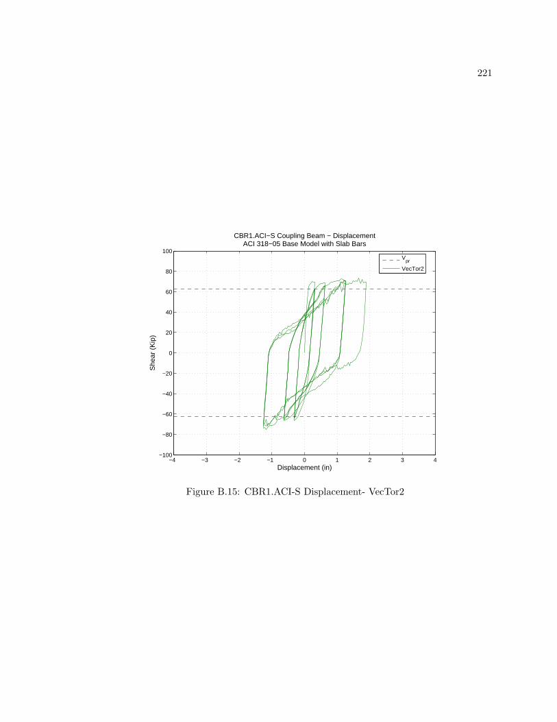
221
−4 −3 −2 −1 0 1 2 3 4−100
−80
−60
−40
−20
0
20
40
60
80
100
She
ar (
Kip
)
Displacement (in)
CBR1.ACI−S Coupling Beam − DisplacementACI 318−05 Base Model with Slab Bars
Vpr
VecTor2
Figure B.15: CBR1.ACI-S Displacement- VecTor2

222
−8 −6 −4 −2 0 2 4 6 8−100
−80
−60
−40
−20
0
20
40
60
80
100
She
ar (
Kip
)
Drift (%)
CBR1.ACI Coupling Beam − DriftACI 318−05
Vpr
VecTor2
Figure B.16: CBR1.ACI Drift- VecTor2
−8 −6 −4 −2 0 2 4 6 8−100
−80
−60
−40
−20
0
20
40
60
80
100
She
ar (
Kip
)
Drift (%)
CBR2.318H Coupling Beam − DriftACI 318H−CH047 Reduced Confinement
Vpr
VecTor2
Figure B.17: CBR2.318H Drift - VecTor2

223
−15 −10 −5 0 5 10 15−100
−80
−60
−40
−20
0
20
40
60
80
100
She
ar (
Kip
)
Drift (%)
CBR2.318H−F Coupling Beam − DriftACI 318H−CH047 Full Confinement
Vpr
VecTor2
Figure B.18: CBR2.318H-F Drift- VecTor2
−15 −10 −5 0 5 10 15−100
−80
−60
−40
−20
0
20
40
60
80
100
She
ar (
Kip
)
Drift (%)
CBR3.318H−M Coupling Beam − DriftACI 318H−CH047 Reduced Full Confinement
Vpr
VecTor2
Figure B.19: CBR3.318H-M Drift - VecTor2

224
−15 −10 −5 0 5 10 15−100
−80
−60
−40
−20
0
20
40
60
80
100
She
ar (
Kip
)
Drift (%)
CBR1.ACI−S Coupling Beam − DriftACI 318−05 Base Model with Slab Bars
Vpr
VecTor2
Figure B.20: CBR1.ACI-S Drift- VecTor2

225
0 0.5 1 1.5 20
10
20
30
40
50
60
70
80
90
100
She
ar (
Kip
)
Displacement (in)
Coupling Beam Comparison
Vpr
CBR1.ACICBR2.318H
Figure B.21: MCBR1.ACI vs. MCBR2.318H - VecTor2
−2 −1.5 −1 −0.5 0 0.5 1 1.5 2−100
−80
−60
−40
−20
0
20
40
60
80
100
She
ar (
Kip
)
Displacement (in)
Coupling Beam Comparison
Vpr
CBR1.ACICBR2.318H
Figure B.22: CBR1.ACI vs. CBR2.318H - VecTor2

226
0 0.5 1 1.5 2 2.5 3 3.50
10
20
30
40
50
60
70
80
90
100S
hear
(K
ip)
Displacement (in)
Coupling Beam Comparison
Vpr
CBR1.ACICBR2.318F
Figure B.23: MCBR1.ACI vs. MCBR2.318H-F - VecTor2
−2 −1.5 −1 −0.5 0 0.5 1 1.5 2−100
−80
−60
−40
−20
0
20
40
60
80
100
She
ar (
Kip
)
Displacement (in)
Coupling Beam Comparison
Vpr
CBR1.ACICBR2.318F
Figure B.24: CBR1.ACI vs. CBR2.318H-F - VecTor2

227
0 0.5 1 1.5 2 2.5 3 3.50
10
20
30
40
50
60
70
80
90
100
She
ar (
Kip
)
Displacement (in)
Coupling Beam Comparison
Vpr
CBR1.ACICBR3.318M
Figure B.25: MCBR1.ACI vs. MCBR3.318H-M - VecTor2
−2 −1.5 −1 −0.5 0 0.5 1 1.5 2−100
−80
−60
−40
−20
0
20
40
60
80
100
She
ar (
Kip
)
Displacement (in)
Coupling Beam Comparison
Vpr
CBR1.ACICBR3.318M
Figure B.26: CBR1.ACI vs. CBR3.318H-M - VecTor2