nonlinear adaptive estimation with application to
TRANSCRIPT

NONLINEAR ADAPTIVE ESTIMATION
WITH APPLICATION TO SINUSOIDAL
IDENTIFICATION
Boli Chen
Department of Electrical and Electronic Engineering
Imperial College London
This dissertation is submitted for the degree of
Doctor of Philosophy
November 2015


I would like to dedicate this thesis to my loving parents and my wife


Declaration of Originality
I hereby declare that this thesis is the result of my own work, all material in this disserta-
tion which is not my own work has been properly acknowledged.
Boli Chen
November 2015


Declaration of Copyright
The copyright of this thesis rests with the author and is made available under a Creative
Commons Attribution Non-Commercial No Derivatives licence. Researchers are free to copy,
distribute or transmit the thesis on the condition that they attribute it, that they do not use it
for commercial purposes and that they do not alter, transform or build upon it. For any reuse
or redistribution, researchers must make clear to others the licence terms of this work.
Boli Chen
November 2015


Acknowledgements
This thesis is the result of research work carried out at the Department of Electrical and
Electronic Engineering, Imperial College London. First and foremost, I would like to express
deepest gratitude to my supervisor, Prof. Thomas Parisini, for giving me the opportunity to
learn substantially from him the passion for science and for his excellent guidance, caring,
patience, and providing me with an excellent atmosphere for doing research. Without his
direction and persistent help this dissertation would not have been completed.
I wish to thank Gilberto Pin from Electrolux Professional S.p.A. for sharing his inspiration
for the topic and for his invaluable advice throughout my works. I am very fortunate to have
had him as a collaborator since the beginning of my PhD. I am indebted to Prof. Shu-Yuen
Ron Hui and Wai Man Ng from Hong Kong University for their collaboration, priceless
advice and assistance in practical implementations. They warmly welcomed me in Hong
Kong when I visited and made a perfect environment for me to perform particular real-time
experiments. A very special thank you to my friend Gabriele Donati from Danieli Automation
S.p.A. where I worked for a very short duration but I gained precious experience on the steel
making industry. I would not have been able to get through to the end of my PhD without the
help I received from all of them.
Thanks to my friends and colleagues, Jingjing Jiang, Yilun Zhou, Yang Wang, Cheng
Cheng, together with all the people of the control and power research group for the perfect
environment you created and the fun we had in the spare times. I strongly believe that this
work would have not been possible without them with whom I shared joyful moments as
well as hard times in the past years.
Finally, I owe deepest gratitude towards my family, for their unceasing encouragement
and support. Without them I could have never achieved any of these results.


Abstract
Parameter estimation of a sinusoidal signal in real-time is encountered in applications
in numerous areas of engineering. Parameters of interest are usually amplitude, frequency
and phase wherein frequency tracking is the fundamental task in sinusoidal estimation. This
thesis deals with the problem of identifying a signal that comprises n (n ≥ 1) harmonics from
a measurement possibly affected by structured and unstructured disturbances. The structured
perturbations are modeled as a time-polynomial so as to represent, for example, bias and
drift phenomena typically present in applications, whereas the unstructured disturbances are
characterized as bounded perturbation. Several approaches upon different theoretical tools
are presented in this thesis, and classified into two main categories: asymptotic and non-
asymptotic methodologies, depending on the qualitative characteristics of the convergence
behavior over time.
The first part of the thesis is devoted to the asymptotic estimators, which typically con-
sist in a pre-filtering module for generating a number of auxiliary signals, independent of
the structured perturbations. These auxiliary signals can be used either directly or indi-
rectly to estimate—in an adaptive way—the frequency, the amplitude and the phase of the
sinusoidal signals. More specifically, the direct approach is based on a simple gradient
method, which ensures Input-to-State Stability of the estimation error with respect to the
bounded-unstructured disturbances. The indirect method exploits a specific adaptive observer
scheme equipped with a switching criterion allowing to properly address in a stable way
the poor excitation scenarios. It is shown that the adaptive observer method can be applied
for estimating multi-frequencies through an augmented but unified framework, which is a
crucial advantage with respect to direct approaches. The estimators’ stability properties are
also analyzed by Input-to-State-Stability (ISS) arguments.
In the second part we present a non-asymptotic estimation methodology characterized by
a distinctive feature that permits finite-time convergence of the estimates. Resorting to the
Volterra integral operators with suitably designed kernels, the measured signal is processed,
yielding a set of auxiliary signals, in which the influence of the unknown initial conditions
is annihilated. A sliding mode-based adaptation law, fed by the aforementioned auxiliary
signals, is proposed for deadbeat estimation of the frequency and amplitude, which are dealt

xii
with in a step-by-step manner. The worst case behavior of the proposed algorithm in the
presence of bounded perturbation is studied by ISS tools.
The practical characteristics of all estimation techniques are evaluated and compared
with other existing techniques by extensive simulations and experimental trials.

Table of contents
Notation xv
Acronyms and Abbreviation xviii
List of figures xxi
1 INTRODUCTION 1
1.1 Background and Motivations . . . . . . . . . . . . . . . . . . . . . . . . . 1
1.2 Literature review . . . . . . . . . . . . . . . . . . . . . . . . . . . . . . . 4
1.2.1 Kalman Filtering . . . . . . . . . . . . . . . . . . . . . . . . . . . 4
1.2.2 Phase-Locked-Loop . . . . . . . . . . . . . . . . . . . . . . . . . 5
1.2.3 Adaptive Notch Filtering . . . . . . . . . . . . . . . . . . . . . . . 7
1.2.4 State-Variable Filtering . . . . . . . . . . . . . . . . . . . . . . . . 9
1.2.5 Adaptive Observers ................................................................................. 10
1.2.6 Estimators with Finite-Time Convergence ................................................ 12
1.3 Aims and Contributions ....................................................................................... 12
1.3.1 Research Challenges in Sinusoidal Estimation ....................................... 12
1.3.2 Contribution of the Thesis ....................................................................... 13
1.3.3 Publications ............................................................................................. 14
1.4 Preliminaries ........................................................................................................ 16
I ASYMPTOTIC ESTIMATORS 21
2 ADAPTIVE OBSERVER APPROACH: THE SINGLE SINUSOIDAL CASE 23
2.1 Introduction .......................................................................................................... 23
2.2 The Pre-Filtering Scheme .................................................................................... 25
2.2.1 Nominal Pre-Filtering System................................................................. 25
2.2.2 Stability of the Pre-Filtering System ....................................................... 28

14ii Table of contents
2.3 Estimation of a Single Sinusoidal Signal ............................................................. 30
2.3.1 ISS Property of the Adaptive Estimator .................................................. 31
2.3.2 Switching Mechanism Based on Excitation Level ................................... 34
2.4 Estimation of Fundamental Frequency of a Generic Periodic Signal .................. 35
2.4.1 Problem Formulation and Preliminaries ................................................. 35
2.4.2 ISS Property of the Adaptation Scheme ................................................. 37
2.5 Digital implementation of the proposed method ................................................. 41
2.5.1 Discretization of the AFP algorithm ....................................................... 41
2.6 Simulation and Experimental Results .................................................................. 44
2.6.1 Simulation Results .................................................................................. 44
2.6.2 Experimental Results .............................................................................. 50
2.7 Concluding Remarks ........................................................................................... 51
3 ADAPTIVE OBSERVER APPROACH: THE MULTI-SINUSOIDAL CASE 53
3.1 Introduction ......................................................................................................... 53
3.2 Problem formulation and preliminaries ............................................................... 54
3.3 Filtered-augmentation-based adaptive observer .................................................. 57
3.4 Stability analysis .................................................................................................. 60
3.4.1 Active adaptation interval of finite duration ........................................... 64
3.4.2 Total dis-excitation phase ........................................................................ 68
3.4.3 Robustness Under Alternate Switching .................................................. 69
3.5 Digital implementation of the proposed method ................................................. 71
3.6 Simulation and Experimental Results .................................................................. 73
3.6.1 Simulation Results .................................................................................. 73
3.6.2 Experimental Results .............................................................................. 79
3.7 Concluding Remarks ........................................................................................... 80
4 STATE-VARIABLE FILTERING-BASED APPROACH 83
4.1 Introduction ......................................................................................................... 83
4.2 Parallel Pre-Filtering System ............................................................................... 84
4.3 Generic Order np + np Pre-Filtering-Based Frequency Estimator ................... 87
4.3.1 Underlying Idea ...................................................................................... 87
4.3.2 Stability Analysis of the Frequency Estimator ........................................ 88
4.3.3 Pre-Filter of Order 3 + 3 ..................................................................... 91
4.4 Order 2 + 2 Pre-Filtering-Based Frequency Estimator ................................... 92
4.4.1 Underlying Idea ...................................................................................... 92

Table of contents xv
4.4.2 Stability Analysis of the Frequency-Adaptation Scheme with 2 + 2
Pre-Filter ...................................................................................................... 93
4.5 Amplitude and Phase Estimation ......................................................................... 98
4.6 Digital implementation of the proposed method .................................................. 99
4.7 Simulation and Experimental Results ................................................................ 100
4.7.1 Simulation Results ................................................................................ 100
4.7.2 Experimental Results ............................................................................ 103
4.8 Concluding Remarks .......................................................................................... 105
II NON-ASYMPTOTIC ESTIMATORS 107
5 FINITE-TIME PARAMETRIC ESTIMATION OF A SINUSOIDAL SIGNAL 109
5.1 Introduction ............................................................................................................. 109
5.2 Preliminaries ........................................................................................................... 110
5.3 Bivariate Feedthrough Non-asymptotic Kernels ................................................ 113
5.4 Finite-time AFP estimation in the presence of bias ........................................... 114
5.5 Finite-time convergence and robustness analysis ............................................... 121
5.5.1 Finite-time convergence ........................................................................... 121
5.5.2 Robustness in the presence of a bounded measurement disturbance . 124
5.6 Digital implementation of the proposed method ................................................ 128
5.7 Simulation results .............................................................................................. 130
5.8 Concluding Remarks .......................................................................................... 135
6 CONCLUSIONS AND FUTURE PROSPECTS 137
6.1 Concluding Remarks .......................................................................................... 137
6.2 Future Work ..................................................................................................................... 138
References 141


Notation
∃ there exists
∀ for all
∈ is an element of
/'. define
! factorial
R real numbers
R≥0 non-negative real numbers
R>0 strictly positive real numbers
Rn real valued n-vectors
Rm×n real valued m × n-matrices
C complex numbers
Z the set of integers
Z≥0 non-negative integers
Z>0 strictly positive integers
∅ empty set
imaginary unit, √
−1
|x| Euclidean norm of x n
∥x∥1 L1 norm |xi| i=1
∥x∥∞ sup norm over a time-varying vector, sup t≥0|x(t)|
inf infimum or greatest lower bound
sup supremum or greatest upper bound
arg argument or solution of an optimization problem
P projection operator
I the identity matrix
0 the null matrix
di
dti u(t) i-th derivative of u(t)

16ii Table of contents
Symbols used in the text
v(t) a measurement perturbed by a structured and unstructured disturbance
y(t) a measurement perturbed by a structured disturbance only
y(t) a stationary single sinusoidal signal
ω angular frequency of a sinusoidal signal
Ω square of the true frequency ω2
a amplitude of a sinusoidal signal
ϕ phase of a sinusoidal signal
d(t) an unstructured disturbance
ωc pre-filter coefficient related to the cutoff frequency of a low-pass filter
Kc damping coefficient of the pre-filter
Ts sampling period
Subscripts, superscripts and accents
x estimate
x estimation error
x0 initial state
x steady state, stationary signal
xi i-th component of the vector x

Acronyms and Abbreviation
AFP Amplitude, frequency and phase
FFT Fast Fourier transform
DFT Discrete Fourier transform
PLL Phase-locked-loop
ANF Adaptative notch filtering
KF Kalman filtering
EKF Extended Kalman filtering
SOGI Second order generalized integrator
OSG Orthogonal signal generator
FLL Frequency locked loop
SVF State-variable filtering
AO Adaptative observer
ISS Input-to-State Stable
B-G Bellman Gronwall (lemma)
LTI Linear time invariant
LTV Linear time varying SISO
Single input single
output MIMO Multi-input
multi-output PE Persistently
exciting
MF Modulating function
BIBO Bounded-input bounded-output
PE Persistency of excitation
SVD Singular value decomposition
w.r.t. With respect to


List of figures
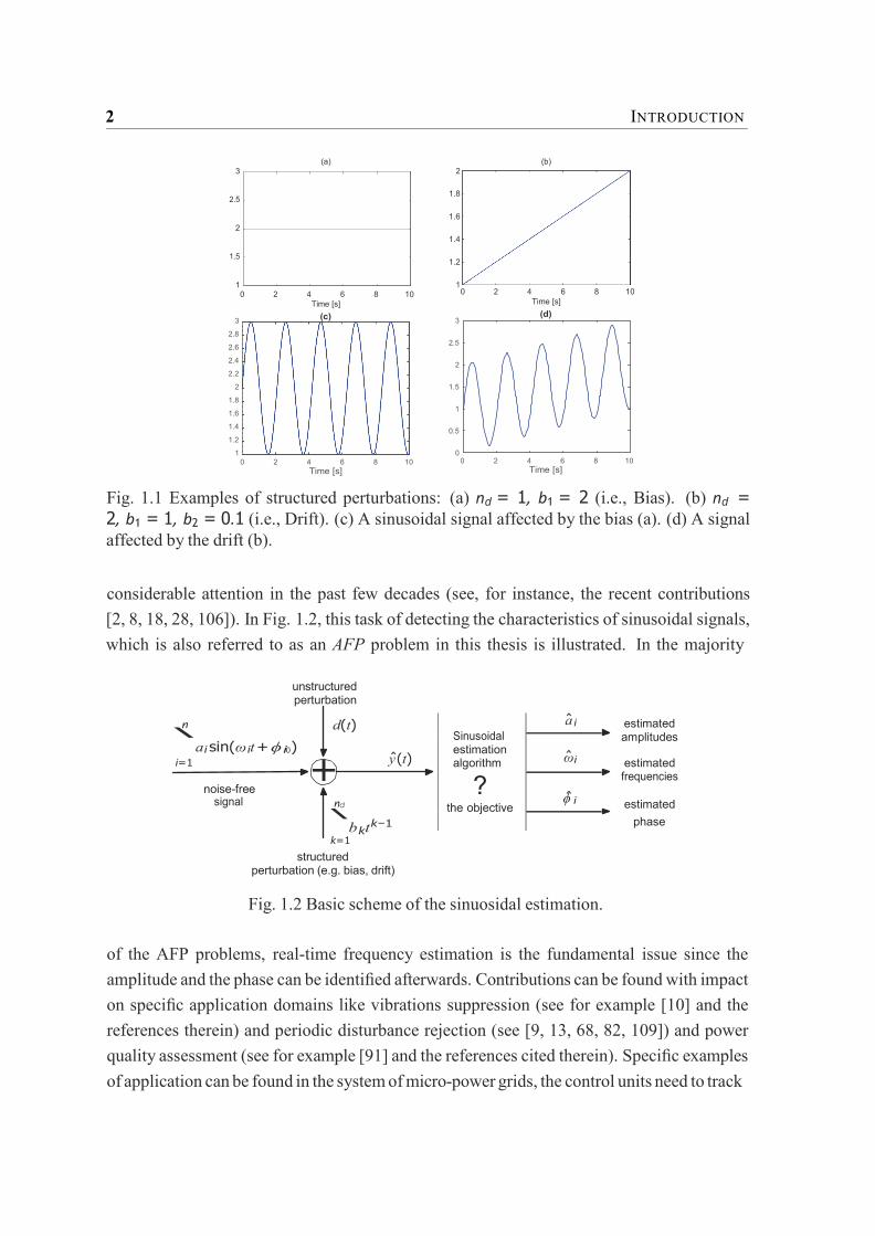
1.1 Examples of structured perturbations: (a) nd = 1, b1 = 2 (i.e., Bias). (b)
nd = 2, b1 = 1, b2 = 0.1 (i.e., Drift). (c) A sinusoidal signal affected by the
bias (a). (d) A signal affected by the drift (b). . . . . . . . . . . . . . . . . 2
1.2 Basic scheme of the sinuosidal estimation. . . . . . . . . . . . . . . . . . . 2
1.3 Mould level control scheme in a steel continuous casting process (drawn
from [40]). . . . . . . . . . . . . . . . . . . . . . . . . . . . . . . . . . . . 3
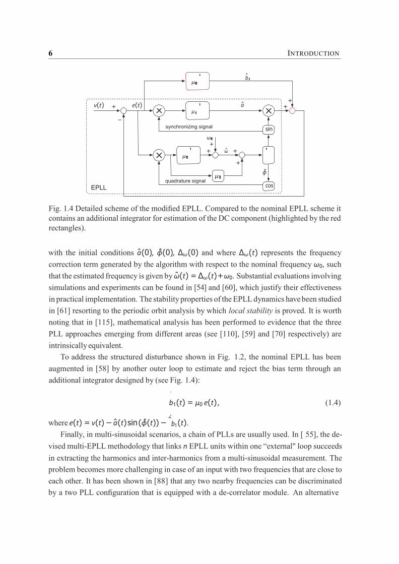
1.4 Detailed scheme of the modified EPLL. Compared to the nominal EPLL
scheme it contains an additional integrator for estimation of the DC compo-
nent (highlighted by the red rectangles). . . . . . . . . . . . . . . . . . . . 6
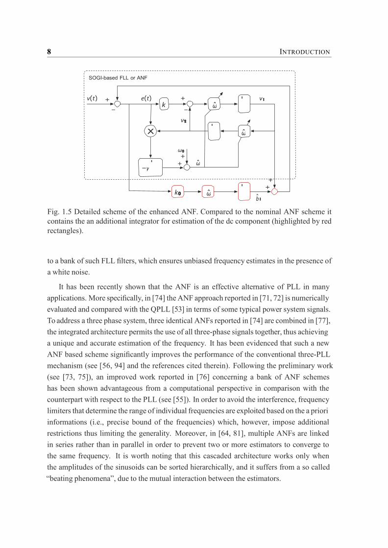
1.5 Detailed scheme of the enhanced ANF. Compared to the nominal ANF
scheme it contains the an additional integrator for estimation of the dc
component (highlighted by red rectangles). . . . . . . . . . . . . . . . . . 8
2.1 Detailed scheme of the proposed pre-filtering system. ......................................... 25
2.2 Estimated frequency obtained by using the proposed AFP method with and
without switching. The switching time-instants are shown by vertical dotted lines.
44
2.3 Left: Instantaneous excitation level ξ(t)⊤ξ(t). Right: Normalized instanta-
neous excitation level Σ(t) ................................................................................... 45
2.4 Time-behavior of log |ω(t)| in the presence of the switching. .............................. 45
2.5 Frequency tracking behavior based on the three sets of ωc and Kc for a biased
sinusoidal signal (top row:ωcKc = 4, bottom row:ωcKc = 6). ........................... 46
2.6 Estimated frequencies from a biased and noisy input signal. ............................... 47
2.7 Comparison of the behaviors in terms of amplitude estimation with adaptive
mechanism (blue line) and unadapted algorithm(red line). .................................. 48
2.8 Estimated sinusoidal signal by the proposed AFP method. .................................. 48
2.9 Measured square waveform. .................................................................................... 49
2.10 Estimated frequency from a noisy square wave. ..................................................... 50

22 List of figures
θpre
θpre
θpre
θ
2.11 Experimental setup and a picture of the experimental setup based on Lab-Volt
Wind power training system. ................................................................................ 50
2.12 Experimental results. Ch1. (bule) Estimated frequency obtained by using
the proposed AFP method (20Hz/Div), Ch2. (pink) Output voltage from the
analog tachometer (500rpm/Div), Ch3. (yellow) line voltage across the wind
turbine generator (50V/Div). Time base: 5s/Div .................................................. 51
2.13 Comparison of the estimated frequency obtained by using the proposed AFP
method and measured prime mover rotational speed. .......................................... 52
3.1 Scheme of the excitation-based switching scheme for enabling/disabling
the parameter adaptation. The transitions to dis-excitation (a) and to active
identification phases (b) have been highlighted. .................................................. 62
3.2 A 2D pictorial representation of the projection-based adaptation. When
|θ(t)| = θ∗
and ˆ (t) points out of the feasible region, then the derivative
of the parameter vector is obtained by projecting ˆ (t) to the tangential
hyperplane. To visually compare the values of the scalar products −θ⊤ (t)
and −θ⊤ (t), consider the projected vectors (a) and (b) respectively .................. 65
3.3 Time-behavior of the estimated frequencies obtained by using the proposed
method (blue) compared with the time behaviors of the estimated frequencies
by [67] (green) and [29] (red). ............................................................................. 73
3.4 Time-behavior of the estimated frequencies by using the proposed method
(blue line) compared with the time behaviors of the estimated frequencies by
the method [67] (green line) and the method [29] (red line). .............................. 74
3.5 Time-behavior of log |ω(t)| with ω = 5 rad/s by using the proposed method
(blue line) compared with the time behaviors of the estimated frequencies by
the method [29] (red line). ................................................................................... 74
3.6 Time-behavior of the estimated amplitudes by using the proposed method
(blue lines) compared to the estimates by the method [29] (red lines). ............... 75
3.7 Time-behavior of log |a1(t)| with a1 = 1 rad/s by using the proposed method
(blue lines) compared to the estimates by the method [29] (red lines). ............... 75
3.8 Estimated sinusoidal signal by the proposed AFP method. ................................. 76
3.9 Frequency tracking behavior with different values of ρ and µ for a noisy
input. Top: ρ = 0.25 (blue lines), ρ = 0.15 (red lines). Bottom: µ = 4 (blue
lines), ρ = 8 (red lines). ................................................................................... 77
3.10 (a) Excitation level λ1(Φ(Ξ(t))); (b) Excitation level λ2(Φ(Ξ(t))); (c) Switch-
ing signal ψ1(t); (d) Switching signal ψ2(t) ......................................................... 78
1
z1
List of figures xxiii
3.11 Time-behavior of the estimated frequencies by using the proposed method.
One of frequency estimates diverges after 120s due to the loss of excitation
in one direction after 120s (see the description on page 77). ................................ 78
3.12 Time-behavior of the estimated amplitudes (blue lines) and the estimated
bias (red line) by using the proposed method. One of the sinusoid vanishes
after 120s, therefore its amplitude decays to 0, resulting in a dis-excitation
phase in one direction (see the description on page 77). ...................................... 79
3.13 The experimental setup. ....................................................................................... 80
3.14 A real-time noisy signal generated by the electrical signal generator .................. 80
3.15 Real-time frequency detection of a single with two frequency contents by
using the proposed method. .................................................................................. 81
3.16 Real-time amplitude detection of a single with two frequency contents by
using the proposed method. .................................................................................. 81
4.1 Detailed scheme of the proposed pre-filtering system. ......................................... 85
4.2 An example plot of the excitation signal z2(t) (blue line) induced by the
stationary sinusoidal signal z1(t) with amplitude az1 (dotted red line), as
well as two horizontal thresholds γf,1(γz (d) + δ) (dotted green line) and
γf,1(γz (d) + δ) + κa2 (green line). ..................................................................... 95
4.3 Time-behavior of the estimated frequency by using the proposed AFP meth-
ods (blue and red line respectively) compared with the time behaviors of the
estimated frequency by the AFP methods [28] (black line), [58] (green line)
and [90] (cyan line)............................................................................................ 101
4.4 Time-behavior of the estimated amplitude by using the proposed AFP meth-
ods (blue and red line respectively) compared with the time behaviors of the
estimated frequency by the AFP methods [28] (black line) and [58] (green
line). ........................................................................................................................ 102
4.5 Estimated sinusoidal signal by the proposed AFP method 2 (blue line). To
appreciate the time-behavior of the estimated signal, the biased noisy input
is depicted (red line), as well as the same signal without the time-varying
bias term (green line).......................................................................................... 102
4.6 Comparison of the behaviors of the proposed AFP method 1 (blue line) and 2
(red line) in the presence of a bounded perturbation within the interval[−5, 5].103
4.7 A real-time 50 Hz sinusoidal voltage signal corrupted by ripples reproducing
the perturbation due to a typical switching device and 4 large spikes per cycle
to reproduce RF interference. ............................................................................ 104
24 List of figures
4.8 Real-time frequency tracking of a sinusoidal signal with a step-wise chang-
ing frequency (50-48-50-52-48 Hz): the time behaviors of the estimated
frequency by the AFP methods [28] (greed line), [58] (red line) and the
proposed method 2 (blue lines).......................................................................... 104
4.9 Real-time frequency tracking of a sinusoidal signal with a step-wise changing
offset: the time behaviors of the estimated frequency by the AFP methods
[28] (greed line), [58] (red line) and the proposed method 2 (blue lines). . . 105
5.1 Plots of the Bivariate Feedthrough Non-asymptotic Kernels and its derivatives
(see (5.14)), for β = β = 1 and n = 3 ............................................................. 114
5.2 Time-behavior of the estimated frequency by using the proposed method and
the method [85] in noise-free scenario: Top: 4-th order Runge-Kutta method,
Bottom: Euler method. ....................................................................................... 131
5.3 Time-behavior of the estimated frequency by using the proposed method
and the method [85] in noisy scenario: Top: 4-th order Runge-Kutta method,
Bottom: Euler method. ....................................................................................... 132
5.4 Time-behavior of the reconstructed pure sine-wave by using the proposed
method in noise-free and noisy scenarios. ......................................................... 133
5.5 Time-behavior of the estimated frequency by using the proposed method
(blue line) compared with the time behaviors of the estimated frequency by
the finite-time method [33] (red line) and the 1-st order SM method [85]
(green line) respectively ..................................................................................... 134
5.6 Time-behavior of the estimated frequency by using the proposed method
(blue line) compared with the time behaviors of the estimated frequency
obtained by the method [79] (red line) respectively. Top: noise-free case.
Bottom: noisy case. ............................................................................................ 135
5.7 Time-behavior of the estimated frequency with different initial conditions
and in a noise-free scenario. Left: the estimator proposed in [79]. Right: the
proposed method. ............................................................................................... 136

i i
k=1
Chapter 1
INTRODUCTION
1.1 Background and Motivations
Consider the signal
n nd
v(t) = ai sin(ϕi(t)) + bktk−1 + d(t)
i=1 k=1 (1.1) ϕ (t) = ω
ϕi(0) = ϕi0
where for a given positive and known integer nd, the term ),nd
bktk−1 represents a time-
polynomial structured exogenous measurement perturbation 1 , with bk unknown for any
k ∈ 1, . . . , nd, and where d(t) characterizes an unstructured perturbation (referred to as
measurement noise in the thesis). The structured measurement disturbances have a practical
interest because they may incorporate bias and measurement drift up to any given order,
the presence of which are commonly acknowledged in several practical applications (see
[35]). For example, physical transducers and A/D converters are often affected by offsets that
correspond to nd = 1, while several sensing devices are influenced by temperature variations
that cause drift phenomena (i.e., nd = 2). Note that in principle nd is the expected order of
the structured perturbations, chosen a-priori by the designer (see Figure 1.1 for examples
with nd = 1 and nd = 2, respectively).
The problem of estimating the amplitudes ai ∈ R>0, the frequencies ωi ∈ R>0 and
the phases ϕi(t) ∈ R, t ∈ R≥0 on the basis of the perturbed measurement (1.1) has drawn
1The given time-polynomial representation includes all the possible structured perturbation in a unified way. A reasonable SNR within a bounded time interval is ensured by proper weighting factors bk . In the
following chapters, we will show that the influence of the structured uncertainty (though unbounded as t → ∞) is removable.
2 INTRODUCTION
0
3
2.5
2
1.5
1
3
2.8
2.6
2.4
2.2
2
1.8
1.6
1.4
1.2
1
(a)
0 2 4 6 8 10
Time [s]
(c)
0 2 4 6 8 10
Time [s]
2
1.8
1.6
1.4
1.2
1
3
2.5
2
1.5
1
0.5
0
(b)
0 2 4 6 8 10
Time [s]
(d)
0 2 4 6 8 10
Time [s]
Fig. 1.1 Examples of structured perturbations: (a) nd = 1, b1 = 2 (i.e., Bias). (b) nd = 2, b1 = 1, b2 = 0.1 (i.e., Drift). (c) A sinusoidal signal affected by the bias (a). (d) A signal
affected by the drift (b).
considerable attention in the past few decades (see, for instance, the recent contributions
[2, 8, 18, 28, 106]). In Fig. 1.2, this task of detecting the characteristics of sinusoidal signals,
which is also referred to as an AFP problem in this thesis is illustrated. In the majority
unstructured perturbation
n d(t)
estimated amplitudes \
ai sin(ωit + ϕi ) i=1
noise-free
signal nd
y(t)
estimated frequencies
estimated
\ bktk−1
k=1
structured perturbation (e.g. bias, drift)
phase
Fig. 1.2 Basic scheme of the sinuosidal estimation.
of the AFP problems, real-time frequency estimation is the fundamental issue since the
amplitude and the phase can be identified afterwards. Contributions can be found with impact
on specific application domains like vibrations suppression (see for example [10] and the
references therein) and periodic disturbance rejection (see [9, 13, 68, 82, 109]) and power
quality assessment (see for example [91] and the references cited therein). Specific examples
of application can be found in the system of micro-power grids, the control units need to track
+
Sinusoidal estimation algorithm
? the objective
a i
ωi
ϕ i

1.1 Background and Motivations 3
the frequency and phase variations of electrical signals with fast dynamics in order to ensure
effective synchronization of the distributed power generators [11, 25, 26]. Moreover, the
massive use of switched-mode power electronics circuits—that inject higher-order harmonics
in the system—requires the development of phase-frequency-tracking techniques that, besides
being fast compared to the time constants of the micro-generators, are robust with respect to
large harmonic distortion and measurement noise. Another example is continuous casting
which is a very important stage of the process of steel manufacturing. A typical setup of
the control architecture in continuous casting plants is depicted in Fig. 1.3 (see [40]). One
Fig. 1.3 Mould level control scheme in a steel continuous casting process (drawn from [40]).
of the most significant control problems in this setup concerns mould level control against
disturbances that may affect the quality of the final products. In particular, the disturbance
caused by the bulging phenomenon generates serious periodic level fluctuation, especially
at high casting speed (see [40] and the references cited therein). Substantial research has
been recently carried on in terms of advanced control schemes improving the rejection of
bulging disturbance. An important component of these control architectures is the estimator
of the bulging disturbance exploiting on-line measurement of the mold level fluctuations. In
this thesis, we concentrate on the design of AFP estimators that are robust against various
disturbances appear in the highlighted challenges, such as structured perturbations modeled
as time-polynomial functions, harmonics and unstructured noises.

4 INTRODUCTION
In the signal processing community there is a rich literature on the problem of frequencies
detection, among which the Prony method, Fourier transform (e.g. FFT and DFT), Chirp
Z transform, the contraction mapping method, adaptive least square methods and subspace
method represent frequently used tools. The principles behind the methods are conceptually
off-line in most cases or are devised for complex exponential sinusoidal signals, hence a
detailed discussion of these methodologies is beyond the scope of the present work and the
reader is referred to [39, 93, 102] and the references cited therein.
On the other hand, a wide variety of approaches for sinusoidal parameter estimation are
already available in the systems and control community. These exploit concepts and tools
such as phase-locked-loop (PLL), state-variable filtering, adaptive observers, adaptive notch
filters (ANF) or Kalman/extended Kalman filters (KF/EKF). A comprehensive review of
some techniques in these categories is carried out in next section.
1.2 Literature review 1.2.1 Kalman Filtering
The Kalman filter appears as one of the most attractive solutions, which has numerous
applications in entire areas of engineering. Ever since the KF and EKF were applied in the
field of frequency detection [101], a large amount of EKF-based frequency trackers have
been proposed in the literature (see, for example [6, 97, 99] and the references cited therein).
In principle, EKF is the nonlinear version of the KF, whereas its process essentially linearizes
the nonlinear dynamics around the previous state estimates without any stability guarantee.
As an example, a representation of the stochastic model for the parametric estimation of a
single sinusoidal signal may be written as
a(k + 1)
1 0 0
s
a(k)
ϕ(k)
ω(k)
+ w1(k)
(1.2)
(k)
where k denotes the discrete time step index with sampling period Ts, a(k), ϕ(k), ω(k) and
y(k) represents the amplitude, phase, angular frequency and the extracted sinusoid at the time
step index k. The random process w1(k) and w2(k) within the state and output equations
are usually white noise characterized by their covariance matrices. In view of (1.2), the
sinusoidal parameters can be retrieved iteratively by implementing the extended Kalman
filter in a straightforward way.
ϕ(k + 1) = 0
1 T ω(k + 1)
y(k) = a(k) sin
0
(ϕ(k))
0
+
1
w2

1.2 Literature review 5
Since the Kalman filter is extremely susceptible to model parameters, the relationship
between its behavior and the tunable parameters has been investigated in [6, 97] to gain
some heuristic guidelines. In the power system community, the KF or EKF still remain the
preferred choice in several applications [91]. For instance, the EKF algorithms proposed
in [50, 95] are shown to be effective in coping with the severely distorted signal in power
systems, although the EKF frequency estimators are characterized by local stability only (see
[98]). Recently, a new EKF-based frequency identifier that relies on a higher order state space
representation, embedding the dynamics of amplitudes is presented in [44]. Compared to the
standard EKF models, the integration of the amplitude’s dynamics significantly improves the
frequency tracking accuracy, especially in the case of a time-varying amplitudes. Last but
not least, structured uncertainties, such as bias or drift, have not been addressed so far in the
context of KF or EKF algorithms.
1.2.2 Phase-Locked-Loop
The Phase-Locked-Loop method and its many variants still represent the most used
approach in many application contexts of electrical and electronic engineering for its ease of
implementation in digital signal processing platforms and its robustness to environmental
and measurement noise (see [3, 41, 48, 103] and the references cited therein). However,
the conventional PLL exhibits the well-known double-frequency ripple phenomenon, which
causes undesired oscillations on the reconstructed signal. In this connection, several modified
PLL architectures are devised in the literature with the aim of improving the conventional
PLL, such as magnitude PLL (MPLL) [110], enhanced PLL (EPLL) [59] and quadrature-
PLL (QPLL) [57]. More specifically, the MPLL consists in providing the PLL of an outer
adaptation loop which is in charge of estimating the amplitude of the input signal, while the
QPLL is based on a mechanism that estimates quadrature amplitudes and frequency of the
input signal. The applicability and benefits of the QPLL in the power and communication
systems are surveyed in [53]. On the other hand, the enhanced PLL (EPLL) [59] along with
its variants [62, 116] represents another class of successful approaches with particular focus
on power and energy applications. A block diagram of the EPLL architecture is shown in
Fig. 1.4, highlighted by the dashed rectangle. The dynamics of the amplitude, frequency and
phase-angle estimates of the EPLL are given equations:
a (t) = µ1 sin (ϕ(t)) e(t) , ∆
ω (t) = µ2 cos (ϕ(t)) e(t) , ϕ (t) = ω0 + ∆ω (t) + µ3 cos (ϕ(t)) e(t) ,
e(t) = v(t) − a(t) sin (ϕ(t)) ,
(1.3)
6 INTRODUCTION
b1
Fig. 1.4 Detailed scheme of the modified EPLL. Compared to the nominal EPLL scheme it
contains an additional integrator for estimation of the DC component (highlighted by the red
rectangles).
with the initial conditions a(0), ϕ(0), Δω (0) and where Δω (t) represents the frequency
correction term generated by the algorithm with respect to the nominal frequency ω0, such
that the estimated frequency is given by ω(t) = Δω (t)+ω0. Substantial evaluations involving
simulations and experiments can be found in [54] and [60], which justify their effectiveness
in practical implementation. The stability properties of the EPLL dynamics have been studied
in [61] resorting to the periodic orbit analysis by which local stability is proved. It is worth
noting that in [115], mathematical analysis has been performed to evidence that the three
PLL approaches emerging from different areas (see [110], [59] and [70] respectively) are
intrinsically equivalent.
To address the structured disturbance shown in Fig. 1.2, the nominal EPLL has been
augmented in [58] by another outer loop to estimate and reject the bias term through an
additional integrator designed by (see Fig. 1.4):
˙ b1(t) = μ0 e(t) , (1.4)
where e(t) = v(t) − a(t) sin (ϕ(t)) − ˙ (t).
Finally, in multi-sinusoidal scenarios, a chain of PLLs are usually used. In [ 55], the de-
vised multi-EPLL methodology that links n EPLL units within one “external" loop succeeds
in extracting the harmonics and inter-harmonics from a multi-sinusoidal measurement. The
problem becomes more challenging in case of an input with two frequencies that are close to
each other. It has been shown in [88] that any two nearby frequencies can be discriminated
by a two PLL configuration that is equipped with a de-correlator module. An alternative
r
μ0 b1
v(t) +
+ e(t) r a + × μ1
− synchronizing signal
ω0
+
× sin
r + ω
× μ2 +
+
r
μ3 ϕ
quadrature signal
EPLL cos

1.2 Literature review 7
solution is given in [43], where the estimates from two identifiers are separated by enforcing
a minimum frequency interval. However, such de-correlation methods are hardly applicable
for a number of harmonics larger than two. In spite of the popularity of the PLL techniques,
the stability results available for the PLL nonlinear AFP algorithms provide, in most cases,
only local stability guarantees, or, when averaging analysis is used, global results are valid
only for small adaptation gains [61, 82, 110].
1.2.3 Adaptive Notch Filtering
Another significant category of techniques is the one concerning algorithms based on the
adaptive notch filtering model that is characterized by constrained poles and zeros. In [92], a
very important ANF estimator is proposed in a lattice-based discrete-time form, while the
continuous time version is introduced in [9] for a typical application to sinusoidal disturbance
rejection with unknown frequency. As reported in [5], the standard ANF model is either
sensitive to the initial condition or subject to biased estimates depending on the positions of
the poles and zeros. To remove such restrictions, a modified ANF-based frequency estimator
that is capable to provide reliable estimates in the presence of colored noise, is presented in
[5]. Thereafter, on the basis of [92], the first globally convergent ANF estimator (i.e., scaled
normalized ANF) has been developed in [49], although the global property is guaranteed
only for sufficiently small adaptation gain. In [71, 72], an improved version of the scaled
normalized ANF that is also known as a second order generalized integrator (SOGI)-based
frequency-locked-loop (FLL) is discussed. The stability results obtained by averaging theory
only ensure local convergence. As can be seen in Fig. 1.5, the DC bias in the measurement
can be handled by an augmented integral loop in addition to the nominal FLL, the revised
ANF turn out to be a SOGI-based orthogonal signal generator (OSG-SOGI) [34, 58]), the
associated frequency adaptation law of which is given by:
˙
b1(t) = k0 ω(t) e(t) , v 1(t) = −ω(t)v2(t) + k ω(t) e(t) , v2(t) = ω(t) v1(t) ,
(1.5)
ω (t) = −γe(t)v2(t) , e(t) = v(t) − v1(t) − b1(t) .
The OSG-SOGI structure is also studied in [28] and [31] for biased sinusoidal signals. In
particular, the frequency adaptation law is integrated into the OSG-SOGI in [31], thus leading
to a new extension, namely a third order generalized integrator-based OSG (OSG-TOGI).
Moreover, the estimation problem for a multi-sinusoidal signal is addressed in [29] resorting
8 INTRODUCTION
Fig. 1.5 Detailed scheme of the enhanced ANF. Compared to the nominal ANF scheme it
contains the an additional integrator for estimation of the dc component (highlighted by red
rectangles).
to a bank of such FLL filters, which ensures unbiased frequency estimates in the presence of
a white noise.
It has been recently shown that the ANF is an effective alternative of PLL in many
applications. More specifically, in [74] the ANF approach reported in [71, 72] is numerically
evaluated and compared with the QPLL [53] in terms of some typical power system signals.
To address a three phase system, three identical ANFs reported in [74] are combined in [77],
the integrated architecture permits the use of all three-phase signals together, thus achieving
a unique and accurate estimation of the frequency. It has been evidenced that such a new
ANF based scheme significantly improves the performance of the conventional three-PLL
mechanism (see [56, 94] and the references cited therein). Following the preliminary work
(see [73, 75]), an improved work reported in [76] concerning a bank of ANF schemes
has been shown advantageous from a computational perspective in comparison with the
counterpart with respect to the PLL (see [55]). In order to avoid the interference, frequency
limiters that determine the range of individual frequencies are exploited based on the a priori
informations (i.e., precise bound of the frequencies) which, however, impose additional
restrictions thus limiting the generality. Moreover, in [64, 81], multiple ANFs are linked
in series rather than in parallel in order to prevent two or more estimators to converge to
the same frequency. It is worth noting that this cascaded architecture works only when
the amplitudes of the sinusoids can be sorted hierarchically, and it suffers from a so called
“beating phenomena”, due to the mutual interaction between the estimators.
SOGI-based FLL or ANF
v(t) + e(t) + v1
k r
ω − −
v2 r
× ω
r
−γ
ω0
+
+ ω
k0
r +
+ ω
b 1

1.2 Literature review 9
For the sake of digital implementation, the discrete-time versions of the continuous-
time FLL filters is introduced in [30] and [105], where the influences of sampling periods
and discretization policies are studied. Although the discretization from a continuous-time
algorithm is a fairly straightforward task, such an analysis is instrumental for the practical
implementation in embedded systems.
1.2.4 State-Variable Filtering
In recent years, significant research activities have been devoted to nonlinear AFP
algorithms involving the use of state-variable filtering (SVF) techniques. The SVF technique
can be illustrated as follows. Consider a linear oscillator generating a single sinusoidal signal:
y(t) = −Ωy(t) , (1.6)
where y(t) /'. A sin (ωt + ϕ0) and Ω /'. ω2. Auxiliary filtering techniques are used to
generate the filtered input’s derivatives for the construction of the frequency adaptation
mechanisms. In this respect, the squared angular frequency is adapted, and then the frequency
is estimated according to
ω(t) =
I
max0, Ω (t) . (1.7)
A simple third-order estimator is presented in [1] for pure sinusoidal signals, and later
it was modified in [2] by adding a leakage correction term to the adaptation law (i.e., the
so-called switching σ modification technique) to prevent estimation drifts in case of perturbed
input. The main drawback of this approach is that the boundedness in a predetermined set
is not guaranteed (“soft projection” is used [51, Chapter 3]). In [90], a minimum-order
frequency estimator for biased sinusoidal signals is introduced; the method offers attenuation
of the high-frequency noise in steady state thanks to the use of switching strategies. However,
the switching algorithm has to be reset if the nominal frequency changes. Finally, in [8],
the same research group presented a fourth-order frequency estimator bringing significant
improvements in robustness compared to [90].
Another class of approaches based on SVF techniques concerns a specific pre-filtering
module composed of a set of identical-cascaded first-order low pass filters. A method
coping with a large class of structured perturbations parameterized in the family of time-
polynomial functions is proposed in [86]. In the spirit of previous work on estimation
of unbiased harmonic signals (see [89]), the robustness of the method against bounded
unstructured perturbations (noise or additive exogenous signals having bounded amplitude)
is characterized by Input-to-State-Stability analysis (also referred to ISS in this thesis). The
ISS-Lyapunov tool also allows to assess the influences of the tunable parameters on the

10
INTRODUCTION
transient performance of the frequency-estimator and on the practical convergence of the
estimates toward a neighborhood of the true values in presence of non-fading perturbations. In
[19, 23], a parallel pre-filtering system (extending the pre-filter used in [86, 89]) is designed.
This enhanced structure allows to simplify the adaptation law introduced in [ 21, 86], while
maintaining the stability properties.
1.2.5 Adaptive Observers
Methods based on adaptive observers yielding the simultaneous estimation of states and
parameters constitute valid alternatives to the aforementioned techniques. The theoretical
properties of these observers have been extensively characterized leading to global or semi-
global stability results (see [7, 45] and the references therein). For example, the recent
paper [20] extends the results presented in [21] (where both structured and unstructured
uncertainties are addressed using suitable pre-filtering techniques) and deals with a “dual-
mode” estimation scheme, in which a switching algorithm (depending on the real-time
excitation level) is integrated into an adaptive observer-based sinusoidal estimator. In
addition, the robustness against bounded unstructured disturbance is proved resorting to ISS
arguments. The dynamic order of this estimator is equal to 6 + nd with nd the order of the
time-polynomial structured perturbations (see (1.1)) that are assumed to possibly affect the
input signal.
It is worth noting that the approaches based on adaptive observers can be extended to
address multi-sinusoidal signals by state augmentation. Specifically, the frequency estimation
problem is addressed by introducing a state space representation of the measured signal,
in which the unknown frequencies are incorporated by a suitable linear parameterization.
Typically, these algorithms do not provide direct estimates of the frequencies. Instead, the
parameter adaptation laws are applied to a set of coefficients of the characteristic polynomial
of the autonomous signal generator system:
n
P (s) = n
(s2 + ωi2) = s2n + θn
k=1
1s2n−2 + · · · + θ1s
2 + θ0
(1.8)
where s is the Laplace variable and (θ0, θ1, · · · , θn−1) are the parameters undergoing adapta-
tion. The frequency estimates are determined as the zeros of the characteristic polynomial.
The first global adaptive observer-based estimator for estimating n frequencies is proposed
in [67] with dynamic order 5n − 1 (5n for the biased case), whereas the dimension of the
adaptive observer is reduced to 3n (3n + 1 for the biased case) in [46, 47, 80, 111] at the price
of a slight degradation of the convergence properties. Moreover, on the basis of the algorithm
−
1.2 Literature review 11
given in [15] dealing with a methodology with minimum order 3n − 1 (3n with bias), the
frequency estimation problems of single sinusoidal signals [16] and multi-frequency signals
[17, 18] with saturated amplitudes are addressed via hybrid systems tools (see [42]).
Alternative schemes in multi-frequency estimation are based on multiple ANFs and PLLs
in parallel. The major issue of such schemes based on banks of adaptive filters in parallel
is the interference between estimators. The adaptive observer approach circumvents this
restriction by estimating the frequencies in a single adaptive system framework, thereby
resulting in an indirect frequency adaptation. The drawback is the computational burden in
the presence of a large number of sinusoids, thus restricting the application in practice. In
this respect, a direct adaptation scheme is designed in [22] with semi-globally exponential
convergence guaranteed thanks to an adaptive observer framework with state-affine linear
parameterization (see [84]).
Theoretically, an arbitrarily large number of sinusoids can be handled by multi-sinusoidal
estimators with properly set order. However, it is commonly acknowledged that the perfor-
mance deteriorates as the number of sinusoids grows. In addition to the above limitation in
multi-sinusoidal estimation, the parameter estimation (e.g. frequencies) problem of a generic
periodic signal with a possibly infinite number of harmonics can not be recast in a traditional
adaptive observer or be solved by multiple PLLs and ANFs. In this respect, most research
efforts only focus on the detection of the fundamental frequency. The PLL and ANF tools,
that are originally conceived for parameter extraction of a single sinusoid, are shown also
to be effective in the presence of a generic periodic signal comprised of arbitrary (possibly
infinite) number of harmonics (see [71, 72, 110]). On the other hand, the internal model
principle proposed by Francis and Wonham [37, 38] also plays an important role in periodic
signal estimation. In [12], an adaptive internal model parametrized by the frequency of the
periodic input is embedded in a fictitious closed-loop system, giving rise to a novel estimation
algorithm. Moreover, the stochastic analysis performed in [113] verifies the robustness of
[12] with respect to additive white noise. Alternatively, [32] deals with an adaptive ‘quasi’
repetitive control (RC) scheme for asymptotic tracking of the fundamental frequency of a
periodic signal. The time-delay of the RC is steered on-line to the period of the input by a
FLL, thereby improving the accuracy by mitigating the effect of the harmonics other than
the fundamental. Nevertheless, the stability analysis of the aforementioned methods is local
and is based on singular perturbation or averaging theory. Recently, a globally convergent
fundamental frequency estimator is proposed [69] using an adaptive observer of order 10 (see
[67]). Moreover, it is shown in [ 24] that another adaptive observer framework presented in
[21] can be generalized, producing a valid alternative for global frequency estimation where
the minimum-dynamic order is reduced to 8.

12
INTRODUCTION
1.2.6 Estimators with Finite-Time Convergence
Despite the numerous sinusoidal estimators available in the literature, only a few of
them can drive the estimation error to 0 within a finite time, which is a desirable feature
in control applications. A deadbeat frequency estimation method is first proposed in [107]
based on the concept of algebraic derivatives, and this methodology is extended in [106]
by processing a measured signal corrupted by an unknown bias. Although the method in
[106] is capable to address the AFP problem with instantaneous convergence by taking
quotients, re-initialization may needed due to the presence of singularities at certain time
instants. This issue has been tackled in [65] and [66] by means of recursive least squares
algorithms, while preserving the deadbeat property. In [108], the algebraic identification
approach [107] is further extended to address the parameter estimation of two sinusoidal
signals from a perturbed measurement. Besides, a modulating function (MF)-based approach
is presented in [33], which allows non-asymptotic frequency detection by processing the
input with suitably truncated periodic functions. Moreover, it has been shown in a recently
proposed FLL framework [34] that the convergence speed and steady state accuracy are
enhanced by employing the MF method [33] for the adjustment of the resonant frequency.
As shown in the very recent papers [83, 87] (dealing with non-asymptotic continuous-
time systems identification), Volterra operators turn out to be an effective tool for finite-time
estimation. Resorting to such kernel based-linear integral operators, a novel finite-time
frequency identifier is presented in [85], implementing a variable-structure adaptation law
based on a sliding mode technique. Instantaneous convergence gets lost in this way, but
a major improvement in robustness to measurement noise is attained while keeping the
deadbeat property with tunable finite-time convergence rate. This is the first finite-time
convergent frequency estimator, the behavior of which is analyzed also in the presence of
unstructured (though bounded) measurement perturbations.
1.3 Aims and Contributions 1.3.1 Research Challenges in Sinusoidal Estimation
We now list the most significant challenges in sinusoidal estimation that this thesis will
address.
• Global stability. Global stability is an important property for sinusoidal estimators.
Although global or semi-global stability has been theoretically proved in methods
based on adaptive observers, this property is not available in some practical AFP tools,
e.g., PLL and ANF due to the use of averaging analysis.

1.3 Aims and Contributions 13
• Robustness and accuracy. The works concerning the AFP estimation in the presence
of bias is vast, yet there is a lack of a comprehensive investigation for the perturbations
other than the bias, e.g. drifts, harmonics and unstructured perturbations, which are
also often encountered in practice.
• Digital implementation. In most cases, AFP methods are devised in a continuous-time
setting which is useful in terms of a possible analog implementation in electronics
and power engineering application contexts. In this connection, one of the issues that
deserve further investigation from a practical perspective is the steady-state bias in the
frequency estimate caused by the discretization of the continuous-time algorithms.
• Persistency of excitation. The persistency of excitation (PE) assumption usually
plays a key role in AFP estimation. It is assumed in standard estimation tools to
guarantee that the estimated sinusoids are sufficiently informative in the presence of
additive disturbances. The loss of excitation is a phenomenon that has not been widely
addressed.
• Multi-sinusoidal signal estimation. Existing methods in the literature are either locally
convergent (refer to PLLs and ANFs in parallel) or less efficient due the indirect
estimation (refer to AO methods).
• Finite-time (instantaneous) estimation . Despite the large number of AFP techniques,
the currently available literature is still short of the deadbeat AFP estimators. This
type of estimators are needed in typical scenarios where the estimates are required
to converge in a neighborhood of the true values within a predetermined finite time,
independently from the unknown initial conditions.
1.3.2 Contribution of the Thesis
The main objective of this thesis consists in providing reliable tools to estimate the
amplitude, frequency and phase of sinusoidal signals in real time from a given perturbed
measurement (1.1) with known n. This includes AFP estimation of a single (i.e., n = 1 in
(1.1)) or multiple sinusoidal signal (i.e., 1 < n < +∞), and even fundamental frequency
tracking of a generic periodic signal that is the sum of an arbitrary (possibly infinite) number
of sinusoids (i.e., n → ∞). The thesis consists of two main parts. Part I regards estimators
with asymptotic convergence property, whereas Part II is devoted to the non-asymptotic
detection of a sinusoidal signal. The contribution of each chapter is briefly outlined in the
following.
In Chapter 2, a specific state variable filtering tool, which plays an important role in
the presented AFP approaches, is introduced (see for example [20, 86]). Thanks to the

14 INTRODUCTION
pre-filtering stage that is configured by cascaded 1-st order low-pass filters, structured per-
turbations with arbitrary order are addressed in a consistent way. Thereafter, we propose
a fundamental frequency estimator that is based on a suitable adaptive observer, which is
characterized by ISS properties in the presence of a class of disturbances, such as structured
perturbations modeled as time-polynomial functions, harmonics and unstructured distur-
bances [20, 24]. The estimator is equipped with a switching criterion enabling the adaptation
only when the excitation condition is fulfilled, thus preventing a possible drift of the estimates
in poor excitation conditions. Although the discretization gives rise to a biased equilibrium,
a post-correction scheme for the proposed methodology is proposed.
In Chapter 3, the basic AO method is extended to identify n unknown frequencies
embedded in a biased signal. In contrast with existing methods, the nonlinear AO allows
the frequency estimates to be updated directly while guaranteeing semi-global stability
property (proved resorting to ISS tools). Moreover, the proposed algorithm is able to tackle
the problem of overparametrization (when the internal model accounts for a number of
sinusoids that is greater than the actual spectral content) or temporarily fading sinusoidal
components by a specific switching criterion: the parameter adaptation scheme with respect
to n frequencies is controlled by an n-dimensional excitation-based switching logic, that
enables the update of a parameter only when the measured signal is sufficiently informative.
Chapter 4 deals with an enhanced pre-filtering configuration, in which the signals pro-
duced by the pre-filtering modules are employed directly for constructing estimation algo-
rithms. In contrast with the AO approach illustrated in Chapter 2, this simplified algorithm
relieves the computation burden whilst still enjoying ISS stability properties with respect to
bounded measurement perturbations.
Finally, in Chapter 5, a deadbeat parametric identifier for biased and perturbed sinusoidal
signals is presented (see [85]). Thanks to Volterra integral operators with suitably designed
kernels, a set of auxiliary signals (regardless of the unknown initial conditions) are produced
by processing the measured signal. These auxiliary signals are exploited for the amplitude
and frequency adaptation, yielding a sliding mode-based methodology that ensures finite-time
convergence of the estimation error. It is worth noting that another significant contribution
consists in the investigation for the worst case behavior of the algorithm in the presence of
bounded additive disturbances; this analysis is currently missing in the literature.
1.3.3 Publications
The research results illustrated in the thesis have been published or are currently under
review in several archival journals . These results have been also presented in several
international conferences. The list of these publications is reported in the following.

1.3 Aims and Contributions 15
• Papers in international journals
1. G. Pin, B. Chen, T. Parisini, and M. Bodson, “Robust Sinusoid Identification
with Structured and Unstructured Measurement Uncertainties,” IEEE Trans.
Automatic Control, vol. 59, no. 6, 2014, pp. 1588-1593.
2. B. Chen, G. Pin, W. M. Ng, C. K. Lee, S. Y. R. Hui, and T. Parisini, “An
Adaptive Observer-based Switched Methodology for Identification of a Perturbed
Sinusoidal Signal: Theory and Experiments,” IEEE Trans. Signal Processing, vol.
62, no. 24, 2014, pp. 6355-6365
3. B. Chen, G. Pin, W. M. Ng, S. Y. R. Hui, and T. Parisini, “A Parallel Pre-
filtering Approach for the Identification of a Biased Sinusoid Signal: Theory and
Experiments,” International Journal of Adaptive Control and Signal Processing,
2015
• Papers included in proceedings of international conferences
1. B. Chen, G. Pin, and T. Parisini, “Adaptive observer-based sinusoid identification:
structured and bounded unstructured measurement disturbances,” in Proc. of the
European Control Conference, Zurich, 2013, pp. 2645-2650.
2. G. Pin, B. Chen and T. Parisini, “A Nonlinear Adaptive Observer with Excitation-
based Switching,” in Proc. of the Conference on Decision and Control, Florence,
2013, pp. 4391-4398.
3. B. Chen, G. Pin, and T. Parisini, “An adaptive observer-based estimator for
multi-sinusoidal signals,” in Proc. of the American Control Conference, Portland,
OR, 2014, pp. 3450–3455.
4. B. Chen, G. Pin and T. Parisini, “Robust Parametric Estimation of Biased Sinu-
soidal Signals: a Parallel Pre-filtering Approach,” in Proc. of the Conference on
Decision and Control, Los Angeles, California, 2014.
5. B. Chen, G. Pin, and T. Parisini, “Frequency Estimation of Periodic Signals: an
Adaptive Observer approach,” in Proc. of the American Control Conference,
Chicago, IL, 2015.
6. G. Pin, B. Chen and T. Parisini, “The Modulation Integral Observer for Linear
Continuous-Time Systems ,” in Proc. of the European Control Conference, Linz,
2015.
16 INTRODUCTION
7. G. Pin, B. Chen and T. Parisini, “Deadbeat Kernel-based Frequency Estimation
of a Biased Sinusoidal Signal,” in Proc. of the European Control Conference,
Linz, 2015.
8. G. Pin, Yang Wang, Boli Chen, and Thomas Parisini, “Semi-Global Direct
Estimation of Multiple Frequencies with an Adaptive Observer having Minimal
Parameterization,” in Proc. of the Conference on Decision and Control, Osaka,
Japan, 2015.
• Papers currently under review
1. B. Chen, G. Pin, W. M. Ng, S. Y. R. Hui, and T. Parisini, “An Adaptive Observer-
based Estimator for Multi-sinusoidal Signals,” IEEE Trans. Automatic Control.
2. G. Pin, B. Chen, and T. Parisini, “Robust Finite-Time Estimation of Biased
Sinusoidal Signals: A Volterra Operators Approach,” Automatica.
3. B. Chen, G. Pin, W. M. Ng, T. Parisini, and S. Y. R. Hui, “A Fast-Convergent
Modulation integral Observer for Online Detection of the Fundamental and
Harmonics in Active Power Filters,” IEEE Trans. on Power Electronics.
1.4 Preliminaries
The purpose of this section is to provide the reader with the basic notations, definitions and
assumptions that are employed throughout the thesis, in order to set a consistent framework.
More specific definitions and assumptions that are not included in this section will be
introduced in the relevant parts of the thesis.
Let M ∈ Rn×m be a matrix. M⊤ denotes the transpose of M while σ(M ) denotes the
set of singular values of M . Let σ(M ) be the maximum singular value of M , whereas σ(M )
be the minimum singular value of M , then ∥M ∥ denotes the induced 2-norm of M , that is
∥M ∥ = σ(M ).
Let M ∈ Rn×n be a symmetric matrix, such that M⊤ = M . The notations M−1, det(M )
and tr(M ) are used to respectively denote the inverse, determinant and trace of M . The set of
eigenvalues values of M is denoted by λ(M ). Similarly, λ(M ) is the maximum eigenvalues
value of M , whereas λ(M ) is the minimum eigenvalues value of M .
Definition 1.4.1 (Positive Definite Matrix) [96] A symmetric matrix M ∈ Rn×n is positive
definite if and only if any one of the following conditions holds:
1. λi(M ) > 0, i = 1, 2, · · · , n.

1.4 Preliminaries 17
1
2. There exists a nonsingular matrix M1 such that M = M1M⊤.
3. Every principal minor of M is positive.
4. x⊤Mx ≥ α|x|2 for some α > 0 and ∀x ∈ Rn
A symmetric matrix M ∈ Rn×n has n orthogonal eigenvectors and can be decomposed as
M = U⊤ΛU (1.9)
where U is a unitary (orthogonal) matrix (i.e., U⊤U = I) with the eigenvectors of M and Λ
is a diagonal matrix composed of the eigenvalues of M . Moreover, a matrix M is negative
definite if −M is positive definite.
Theorem 1.4.1 [52] Let M ∈ Rn×n. The following statements are equivalent:
1. all the eigenvalues of M have negative real part;
2. for all matrices Q = Q⊤ > 0 there exists an unique solution P = P⊤ > 0 to the
following (Lyapunov) equation:
M⊤P + PM + Q = 0
Definition 1.4.2 [63] A continuous function α(r) : R≥0 → R≥0 belongs to the class K if it
is continuous, strictly increasing and α(0) = 0. If, in addition limr→∞ α(r) = ∞ then it
belongs to the class K∞.
Definition 1.4.3 [63] A continuous function β : R≥0 × R≥0 → R≥0 belongs to the class KL
if, for any fixed t ∈ R≥0, the function β(·, t) is a K-function with respect to the first argument
and if, for any fixed r ∈ R≥0, the function β(r, t) is monotonically decreasing with respect to
t and limt→∞ β(r, t) = 0.
Definition 1.4.4 (Piecewise Continuity) [63] A function f : [0, ∞) → R is piecewise
continuous on [0, ∞) if f is continuous on any finite interval [t0, t1] ⊂ [0, ∞) except for a
finite number of points.
Definition 1.4.5 (Lipschitz) [96] A function f : [x, x] → R is Lipschitz on [x, x] if |f (x1) −
f (x2)| ≤ κ|x1 − x2|, ∀x1, x2 ∈ [x, x], where κ ≥ 0 is a constant referred to as the Lipschitz
constant.

18 INTRODUCTION
1
0
≥0
Consider the following dynamical system
x = f (x, u) (1.10)
with x ∈ Rn, u ∈ Rm, f (0, 0) = 0 and f (x, u) locally Lipschitz in Rn × Rm.
Definition 1.4.6 (ISS) [63] The system (1.10) is ISS (Input-to-State Stable) if there exist a
KL-function β(·, ·) and a class K-function such that, for any input u ∈ Rm and any initial
condition x0 ∈ Rn, the trajectory of the system verifies
|x(t)| ≤ β(|x0|, t) + γ(∥u∥∞) (1.11)
Definition 1.4.7 (ISS-Lyapunov Function) [63] A function V : Rn → R of class C1 is
an ISS-Lyapunov function for (1.10) if there exist three K∞-functions α(·), α(·), α(·) and a
K-function X (·) such that
α(|x|) ≤ V (x) ≤ α(|x|), ∀x ∈ Rn (1.12)
and
|x| ≥X (|u|) ⇒
∂ V f (x, u) ≤−α(|x|), ∀x ∈Rn
, ∀u ∈Rm
(1.13)
Theorem 1.4.2 ([63]) The system (1.10) is ISS if and only if it admits an ISS-Lyapunov
function. D
Definition 1.4.8 [96] The set Lq, q ∈ 1, 2, · · · , q < ∞, consists of all the measurable
functions f : R≥0 → R that satisfy
r ∞
∥f (t)∥qdt < ∞ 0
Moreover (( ∞
∥f (t)∥qdt)
q is the Lq norm of the function f ∈ Lq. If q = ∞, the set L
consists of all measurable functions f : R≥0 → R which are bounded, namely
with norm ∥f ∥∞ = supt∈R>0
∥f (t)∥
sup t∈R>0
∥f (t)∥ < ∞
Lemma 1.4.1 (Bellman-Gronwall’s Inequality-differential form) Let T = [t0, t1]. Sup-
pose g: T → R and h: T → R are continuous, and suppose u: T → R is in C1(T ) and
∂x
∞

1.4 Preliminaries 19
t0 ≤ 0
r t
satisfies
Then
u (t) ≤ g(t)u(t) + h(t) for t ∈ T , and u(t0) = u0.
u(t) u er t
g(s)ds
r t + e s
g(τ )dτ h(s)ds (1.14) t0
Moreover, let us introduce following assumptions on the main problem formulated in (1.1):
Assumption 1 (Boundedness of the Disturbance) The unstructured measurement noise
d(t) defined in (1.1) is subject to an a-priori known bound d, that is
|d(t)| ≤ d , t ∈ R≥0 . (1.15)
Assumption 2 (Boundness and Uniqueness of the Frequencies) The frequencies of the si-
nusoids in (1.1) are all unique strictly-positive time-invariant parameters, bounded by a
positive constant ω, such that ωi > 0, ωi = ωj for i = j and
ωi < ω, ∀i ∈ 1, · · · , n. (1.16)


Part I
ASYMPTOTIC ESTIMATORS


Chapter 2
ADAPTIVE OBSERVER APPROACH: THE
SINGLE SINUSOIDAL CASE
2.1 Introduction
In this chapter, the AFP estimation of a single sinusoidal signal from a measurement
affected by structured and unstructured disturbances is addressed. Let us recall the generic
sinusoidal measurement (1.1) and let n = 1, consequently forming the available signal as
follows: nd
v(t) = y(t) + bktk−1 + d(t) , t ∈ R
k=1
, (2.1)
where y(t) represents the stationary sinusoidal signal described by
y(t) = a sin(ϕ(t)) ,
ϕ (t) = ω , ϕ(0) = ϕ0 ,
t ∈ R≥0 , (2.2)
with unknown amplitude, angular frequency and phase respectively denoted by a, ω, and ϕ,
wherein ω < ω according to Assumption 2. Note that the choice of nd is not unique. For
instance, a bias is involved with all nd ≥ 1. Therefore, in case of a sensing devise affected by
uncertain perturbations, a proper choice of nd has to be carried out depending on the a-priori
knowledge about the possible structured uncertainties in the specific application. In addition,
d(t) is subject to the constraint (1.15) given in Assumption 1.
In the works [21, 86, 89], a set of cascaded first-order low-pass (LP) filters, called “pre-
filter” is exploited with the aim of both canceling the effect of structured “time-polynomial”
perturbations (such as bias and linear drift) and obtaining auxiliary signals for AFP detection.
≥0

24 ADAPTIVE OBSERVER APPROACH: THE SINGLE SINUSOIDAL CASE
1,n
The said signals can be used either directly (see [89] and [86]) or indirectly (see [21]) to
estimate the unknown parameters of the measured sinusoid with high noise immunity.
This chapter deals with a class of sinusoidal estimators that employ the auxiliary pre-
filtered signal indirectly resorting to a specific adaptive observer system. The behavior of
the approach against various types of disturbances is characterized by a comprehensive
robustness analysis. In Sec. 2.3, we will start from a problem formulated by (2.1) based
on some preliminary results in [21], a “dual-mode” estimation scheme is dealt with by
incorporating a switching algorithm (depending on the real-time excitation level) into an
adaptive observer-based sinusoidal estimator. In comparison with the typical adaptive
estimators relying on an integral-type persistency of excitation condition (see, for instance,
[8, 67, 111]), the devised method allows to check the excitation level in real-time which
might be advantageous from a computational perspective. The stability properties of the
devised method are rigorously analyzed in terms of ISS arguments thus coping with bounded
measurement noise.
In Sec. 2.4, we study the behavior of the introduced AO estimator in the scenario where
the input is corrupted by a series of harmonics of the fundamental. Consider a bounded
piecewise continuous periodic signal y(t) of unknown frequency ω, that can be expressed in
terms of its Fourier harmonic components as follows:
y(t) = a0
2 a0
∞
+ [a1,n cos (nωt) + a2,n sin (nωt)] n=1
(2.3) /'. + a1,n cos (ωt) + a2,n sin (ωt) + h(t)
2
= a0
2
2 1,n
2 2,n sin (ωt + ϕ0) + h(t), t ∈ R≥0
in which ϕ0 = arctan (a1,n/a2,n) and h(t) collects all the high order harmonics of y(t). We
assume that a2
2 2,n > 0. Our objective consists in estimating the fundamental frequency
of y(t) from a noisy measurement v(t) = y(t) + d(t), which can be subsumed into (1.1)
with the number of the frequencies tend to infinity: n → +∞. Assuming that the amplitude
of the fundamental is larger than that of the high-order harmonics, we will investigate the
convergence of the AO technique by considering the high-frequency content as a bounded
perturbation (i.e.,∥h∥∞ ≤ h, h ∈ R≥0) whose effect on the estimated frequency can be
bounded by adopting a deterministic worst-case viewpoint. Compared with [69], where the
availability of a pure periodic signal y(t) is assumed, the ISS analysis performed in this work
encompasses also the presence of a bounded measurement noise, i.e., d(t) other than the
harmonics. By explicitly expressing the ISS asymptotic gains of the estimator in terms of the
tuning parameters of the algorithm, it is possible to highlight the influence of each parameter
+ a I
+ a
+ a

2.2 The Pre-Filtering Scheme 25
k=1
on the accuracy of the estimates. The practical characteristics of the estimator are evaluated
and compared with other existing tools by extensive simulation trials in Sec. 2.6.
2.2 The Pre-Filtering Scheme
2.2.1 Nominal Pre-Filtering System
To deal with the structured perturbation term),
nd
bktk−1 appearing in (2.1), we extend
the state variable filtering tool proposed in [89] (see also the alternative GPI observer
approach [27]) to compute the unavailable time-derivatives of y(t) that are needed to remove
the effect of structured perturbations from the AFP estimates. To this end, we first address
the problem for the noise-free signal
nd
y(t) = y(t) + '\"
bktk−1 , t ∈ R k=1
. (2.4)
A block diagram of the proposed pre-filter’s architecture [86] is shown in Fig. 2.1. In the
Fig. 2.1 Detailed scheme of the proposed pre-filtering system.
simplified setting given by (2.4), we adopt a np-th order pre-filter, the dynamics of which
obey ( x 1(t) = ωc (Kcy(t) − x1(t))
x k (t) = ωc (Kcxk−1(t) − xk (t)) , ∀k ∈ 2, . . . , np, (2.5)
where xk (0) = xk 0, k ∈ 1, . . . , np; ωc and Kc are positive parameters to be selected by
the designers. In qualitative terms, ωc determines the cut-off frequency while Kc ∈ (0, 1]
acts as a damping coefficient. More details of parameter tuning and the benefit of using a
non-unity DC gain Kc will be discussed in Sec. 2.6 (see Fig. 2.5). In the following, we will
s + ω c s + ω q filters
c s + ω c
x q (t)
xq (t)
y(t)
dq
dtq xq (t)
≥0

26 ADAPTIVE OBSERVER APPROACH: THE SINGLE SINUSOIDAL CASE
0
show that for all np ≥ nd, there exists a class of computable auxiliary signals derivatives that
are independent of the structured disturbance in steady state.
Defining x(t) /'. [ x1(t) . . . xnp (t)]⊤, a state-space realization of the filter evolving from
np
arbitrary initial conditions x0 /'. [ x10 . . . xnp ]⊤ ∈ R is
( x (t) = Ax(t) + B y(t)
xnp (t) = Cx(t)
(2.6)
where −ωc 0 · · · · · · 0
Kcωc
. . . . ..
A = Kcωc −ωc .
. . , B =
0 , (2.7)
. . . . . .
. . . ...
...
...
. . . . . .
. . . 0
0
and
0 · · · 0 Kcωc −ωc
C = I
0 · · · 0 1 1
. (2.8)
In view of the proposed filter’s structure, it follows that
C Ak B = 0, ∀k ∈ 0, . . . , np − 2 .
d2 dnp
Then, the time-derivatives x np (t), dt2 xnp (t), · · · , dtnp xnp (t) can be computed as follows:
dk
dtk xnp (t) = CA
kx(t), ∀k ∈ 1, . . . , np − 1 ,
(2.9)
dnp
dtnp xnp (t) = CA
np−1 (Ax(t) + By(t)) .
Now, the Laplace transform of xk, ∀k ∈ 1, 2, · · · , np is
L[xk ](s) = Hk (s)L[y](s) with Hk (s) =
ωk Kk c c .
(s + ωc)k
Neglecting the initial conditions of the internal filter’s states, the Laplace transform of the
auxiliary signal is:
L[xnp ](s) = Hnp (s)a s sin(ϕ0) + ω cos(ϕ0)
s2 + ω2 + Hnp (s)
nd
k=1
1
bk (k − 1)! sk
0
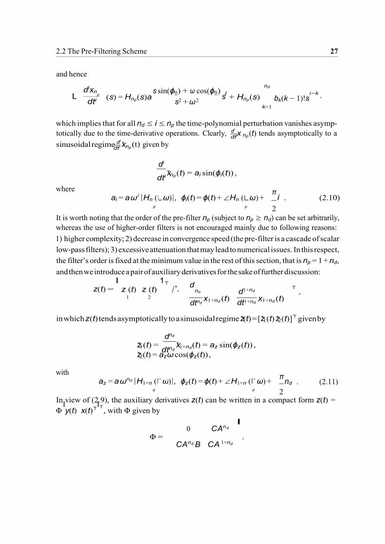
2.2 The Pre-Filtering Scheme 27
p
dti
dti
and hence
dixn
L dti
(s) = Hnp (s)a
s sin(ϕ0 ) + ω cos(ϕ0 ) i
s2 + ω2 s
+ Hnp (s)
nd
k=1
bk (k − 1)!s i−k .
which implies that for all nd ≤ i ≤ np the time-polynomial perturbation vanishes asymp-
totically due to the time-derivative operations. Clearly, di
x (t) tends asymptotically to a
sinusoidal regime di
x
where
(t) given by
di
dti xnp (t) = ai sin(ϕi(t)) ,
π
ai = a ω i |Hn ( )|, ϕi(t) = ϕ(t) + ∠Hn ( ) + i . (2.10) p p 2
It is worth noting that the order of the pre-filter np (subject to np ≥ nd) can be set arbitrarily,
whereas the use of higher-order filters is not encouraged mainly due to following reasons:
1) higher complexity; 2) decrease in convergence speed (the pre-filter is a cascade of scalar
low-pass filters); 3) excessive attenuation that may lead to numerical issues. In this respect,
the filter’s order is fixed at the minimum value in the rest of this section, that is np = 1 + nd,
and then we introduce a pair of auxiliary derivatives for the sake of further discussion:
z(t) = I
z (t) z (t) 1⊤
/'. d
d1+nd ⊤ ,
1 2
dtnd x1+nd (t)
dt1+nd x1+nd (t)
in which z(t) tends asymptotically to a sinusoidal regime z(t) = [z1(t) z2(t)]⊤ given by
dnd
z1(t) = dtnd
x1+nd (t) = az sin(ϕz (t)) ,
z2(t) = azω cos(ϕz (t)) ,
with az = a ωnd |H1+n ( )|, ϕz (t) = ϕ(t) + ∠H1+n ( ) +
π
nd . (2.11) d d 2
In view of (2.9), the auxiliary derivatives z(t) can be written in a compact form z(t) =
Φ ly(t) x(t)⊤
l⊤, with Φ given by
0 CAnd
l
Φ = . CAnd B CA 1+nd
np
np
nd

28 ADAPTIVE OBSERVER APPROACH: THE SINGLE SINUSOIDAL CASE
d d
∞
⊤
As a final remark, it is immediate to see that the sinusoidal regimez(t) can be described
in terms of the following simple state equations: (
z(t) = Az z(t) + ΩGz z(t)
z1(t) = Cz z(t) (2.12)
by setting the initial conditions as
z(0) = I
az sin (ϕ0 + ∠H1+n ( ω) + nd
\ azω cos
(ϕ0 + ∠H1+n ( ) +
2 nd
\ 1 ,
2
with Ω = ω2, Az =
0 1 l
0 0
, Gz =
0 0
l
−1 0 , and Cz =
I 1 0
1.
2.2.2 Stability of the Pre-Filtering System
Consider again the perturbed measurement signal v(t) given by (2.1), we denote by x(t)
the actual state vector of the pre-filter, driven by the noisy signal v(t) and evolving from an
arbitrary initial condition x0 as follows: (
x (t) = Ax(t) + Bv(t) ,
x1+nd (t) = Cx(t) . (2.13)
Introducing the error vector with respect to x(t), which is driven by a choice of the filter’s
initial state x0 such that auxiliary signal derivative z(t) matches the stationary sinusoidal
behavior since the very beginning,
x(t) /'. x(t) − x(t)
and noticing that d(t) = v(t) − y(t), the dynamics of x(t) can be written as:
( x (t) = Ax(t) + B d(t) ,
x(0) = x0 − x0 .
(2.14)
The following results can be proved:
Theorem 2.2.1 (ISS of the pre-filtering system) Given the sinusoidal signal y(t) and the
perturbed measurement v(t) (2.1), the error dynamic of the pre-filtering system (2.13) is ISS
w.r.t. any additive disturbance signal d(t) ∈ L1 . D
π π

2.2 The Pre-Filtering Scheme 29
1
Proof: Being A Hurwitz, there exists a positive matrix P that solves the the Lyapunov
equation P A + A⊤P = −I. Let W (x) /'.
α1, α2 ∈ R>0 such that
x⊤P x; then there exist two positive scalars
α1|x|2 ≤ x⊤P x ≤ α2|x|
2, ∀x
The derivative of W along the system’s state trajectory satisfies
For any 0 < ϵ < 1, let
∂ W
∂x (Ax + Bd) ≤ −|x|2 + 2 ∥P ∥ |B| |d| |x|.
2 ∥P ∥ |B|
X (s) /'.
with r ∈ R≥0. It is easy to show that
r. 1 − ϵ
|x| ≥ X (|d|) ⇒ ∂ W
∂x (Ax + B d) ≤ −|x|2,
and that the system is ISS with asymptotic gain
γx(r) = α −1 α2 X (r).
In view of the ISS property of the linear auxiliary filter (2.36), for any arbitrary ν ∈ R>0
and for any finite-norm initial error x0, the error vector x(t) enters in a closed ball of radius
γx(∥d∥∞) + ν ≤ γx(d) + ν in finite time Tx0,ν . •
Now, let z(t) be the vector of the computable perturbed counterpart of z(t):
z(t) = Φ[v(t) x(t)⊤]⊤ , (2.15)
the boundedness of z(t) is characterized by the following corollary:
Corollary 2.2.1 Given the sinusoidal signal y(t) and the perturbed measurement v(t) (2.1),
if the pre-filtering system (2.6) is applied, then the available auxiliary signal vector z(t)
derived by (2.15) is bounded. D
Proof: Using (2.1) and (2.15), it is immediate to conclude that the vector z(t) /'. z(t) − z(t)
enters in finite-time Tδz = Tx0,ν (for the sake of simplifying the notation, we have dropped
the dependence of the reach-time Tδz on initial conditions) in a closed hyper-sphere of radius
γz (d) + δ centsred at the origin, with
γz (s) = φ(γx(r) + r), ∀r ∈ R≥0, δ = φυ (2.16)

30 ADAPTIVE OBSERVER APPROACH: THE SINGLE SINUSOIDAL CASE
d
where φ ≥ ||Φ||.
From the equality z(t) = z(t) + z(t), it turns out that the proven boundedness of both
z(t) and z(t) implies the boundedness of the z(t), thus ending the proof. •
2.3 Estimation of a Single Sinusoidal Signal
In view of (2.12), by introducing the estimated squared-frequency Ω (t) = ω(t)2, the filter
output z(t) is used as the input for the following adaptive observer having internal state z(t):
ˆ
z(t) = (Az − Lz Cz )z(t) + LCz(t) + Gz z(t)Ω (t) + ξ(t)Ω(t) ξ (t) = (A — L C )ξ(t) + G z(t)
, (2.17) ˆ
z z z z ˆ
Ω(t) = −µξ(t)⊤(z(t) − z(t))
where µ ∈ R≥0 is an arbitrary positive constant and L is the observer gain such that
(Az − Lz Cz ) is Hurwitz. Roughly speaking, increasing µ corresponds to an acceleration
in the convergence rate of the estimation error, whereas the accuracy is degraded due to a
typical trade-off between asymptotic accuracy and convergence speed (see Fig. 2.4). Finally,
ω(t) =
I
max0, Ω (t) . (2.18)
Given Ω (t) and z(t) and assuming, for the moment, that
Ω (t) > 0, ∀ t , (2.19)
then, the filtered regime amplitude and phase (az, ϕz ) defined in (2.11) are estimated by
az (t) =
I
(Ω (t)z1(t)2 + z2(t)2)/Ω (t), (2.20a)
ϕz (t) = ∠ [z2(t) + ω(t)z1(t)] . (2.20b)
Thanks to the availability of az , ω, ϕz related to the auxiliary signal z1(t), from (2.11), with
the assumption (2.19), we obtain the following estimates of the original parameters:
a(t) = az (t) 1
, (2.21a)
ω(t)nd |H1+n ( ω(t))|
π
ϕ(t) = ϕz (t) − ∠H1+nd ( ω(t)) − nd 2
. (2.21b)

2.3 Estimation of a Single Sinusoidal Signal 31
c
1 2
2
After some algebra, we finally get:
a(t) =
az (t)
ω(t)nd
(ω2 + ω(t)
2)
1
ωcKc
1+nd , (2.22a)
ϕ(t) = ϕz (t) + (1 + nd) arctan
ω(t)
ωc
π
− nd 2
. (2.22b)
Assumption (2.19) is needed for (2.20a) and (2.21a) to be well-posed at any time-instant t.
Let us remove the need for (2.19) by resorting to the following adaptive amplitude estimators.
To this end, from the equality (2.20a), we define the time-varying residual that depends on
the frequency estimate Ω (t) and on the instantaneous values of the filtered signals z1(t) and
z2(t):
R(az (t), t) /'. az (t)ω(t) −
I
Ω (t)z1(t)2 + z1(t)2 ,
the following adaptation law stemming from gradient algorithm [96] can be designed
a z (t) = −µa
∂R(az , t)
∂az R(az , t)
= −µaω(t) ω(t)az (t) −
/(Ω (t)z (t)2 + z (t)2
\ ,
(2.23)
where the estimates is clipped by: az (t) = max0, az (t), az (0) = az (0) = 0 and µa ∈ R>0
is a tuning gain set by the designer to steer R(az (t), t) to 0 asymptotically. It is worth to point
out that µa plays a similar role as µ does in (2.17), hence the ways of tuning are likewise
referred to Fig. 2.4. Thanks to (2.23), the estimate of the filtered amplitude az (t) can be
computed through (2.23) without the need of assuming (2.19). Using az (t) provided by
(2.23), the following adaptive algorithm can be finally used to estimate the original amplitude:
a (t) = −µaω(t)nd a(t)ω(t)nd −
az (t)
|H1+nd ( ω(t))|
, (2.24)
with a simple clipping: a(t) = max0, a(t) and a(0) = a(0) = 0. In Section 2.6, the
amplitude estimate given by (2.24) is evaluated by simulations.
2.3.1 ISS Property of the Adaptive Estimator
In order to address the stability of the adaptive observer, let us introduce some instrumen-
tal error variables: z(t) /'. z(t) − z(t), Ω (t) /'. Ω (t) − Ω, and ζ(t) /'. z(t) − ξ(t)Ω (t). Then,

32 ADAPTIVE OBSERVER APPROACH: THE SINGLE SINUSOIDAL CASE
Ω(
we have:
z(t) = (Az − Lz Cz )z(t) + (Lz Cz + ΩGz )z(t) + Ω (t)Gz z(t) + ξ(t) ˙
t) , (2.25a)
Ω˙
(t) = −µξ(t)⊤ξ(t)Ω (t) + µξ(t)⊤ (z(t) − ζ(t)
\ , (2.25b)
ζ˙(t) = (Az − Lz Cz )ζ(t) + (Lz Cz + ΩGz )z(t). (2.25c)
The following assumption is needed to address the convergence analysis of the estimator.
Assumption 3 The solution ξ(t) of ξ (t) = (Az − Lz Cz )ξ(t) + Gz z(t) is instantaneously
persistently exciting (IPE) in the sense that there exist a positive constant ϵ such that
ξ(t)⊤ξ(t) > ϵ, ∀t ≥ 0. (2.26)
It is worth noting that, instead of the typical integral type of persistency of excitation
condition (see, for instance, [8]) that requires on-line buffering by a moving time window, the
exploitation of the above IPE condition in the switching algorithm presented in Section 2.3.2
greatly enhances the on-line implementation of the adaptive estimation technique, because
the IPE condition is easily computable at each time instant without any delay (the reader is
referred to Example 1 in Section 2.6 for an instance).
Now, the following basic stability result is given and proved.
Theorem 2.3.1 (ISS of the adaptive observer system) Suppose that Assumption 1, 3 hold.
Then, given the sinusoidal signal y(t) generated by (2.2) and the perturbed measurement
model (2.1), the adaptive observer as well as the frequency estimator given by (2.13),
(2.15) and (2.17) are ISS with respect to any additive measurement perturbation such that
|d(t)| ≤ d .
D
Proof: Consider the candidate Lyapunov function Vζ = ζ(t)⊤Qζ(t), where Q is a positive
definite matrix solving the linear Lyapunov’s equation:
Q(Az − Lz Cz ) + (Az − Lz Cz )⊤Q = −I. (2.27)
In view of the dynamics of ζ(t) obeying (2.25c), the time-derivative of the Lyapunov function
verifies the inequality
∂ Vζ ζ˙(t) ≤ −|ζ(t)|2 + 2||Q|| ||L C + ΩG || |z(t)| |ζ(t)| . (2.28)
∂ζ z z z

2.3 Estimation of a Single Sinusoidal Signal 33
2
˜
k
s
Hence, Vζ is an ISS-Lyapunov function for ζ(t) w.r.t. the z(t). Moreover, the dynamics of z(t)
is ISS w.r.t. disturbance d(t), so that ζ(t) is, in turn, ISS w.r.t. d(t) such that |d(t)| ≤ d. Now,
let VΩ = 1 Ω (t)2 be a candidate Lyapunov function of the frequency-estimation subsystem.
Then, the derivative of VΩ verifies the inequality
∂ VΩ Ω˙ (t) ≤ −µ|ξ(t)|2|Ω (t)|2 + µ|ξ(t)||z(t) − ζ(t)| |Ω (t)| . (2.29)
∂Ω
In view of (2.29), Assumption 3, and the boundedness of |ξ(t)| (it is immediate to show that
the dynamics of ξ(t) is ISS w.r.t. the bounded input z(t)), we have that Ω (t) is ISS w.r.t. ζ(t)
and z(t), which are all proven to be ISS w.r.t. d(t) such that |d(t)| ≤ d.
Finally, the identity z(t) = ζ(t) + ξ(t)Ω (t), and the boundedness of |ξ(t)| together imply
that also the state-estimation error z(t) is ISS w.r.t. d(t) such that |d(t)| ≤ d. •
Next, we are going to establish the relationship between the excitation condition and the
observer poles location.
Lemma 2.3.1 (Observer Poles and Excitation) Assume that in the noise-free mode of be-
haviour (that is, d(t) = 0), the poles of Az − Lz Cz are assigned to (p1, p2), where p1, p2 =
e1 ± 2 with e1 ∈ R<0, e2 ∈ R, such that
e2 2
1 > e2, e1 ∈ R<0, e2 ∈ R . (2.30)
Then, the IPE condition (2.26) is verified for any t > 0 by any sinusoidal signal.
Proof: In stationary conditions, by defining Bξ = [0 − 1]⊤
, the dynamic equation of ξ(t), in
absence of noise can be rewritten as
ξ (t) = (Az − Lz Cz )ξ(t) + Bξ z1(t) ,
with ξ(0) = 0. Then, in the Laplace domain we have ξk (s) = Hξ,k (s)z1(s), k ∈ 1, 2,
where Hξ,k (s) = ι⊤(sI − Az + Lz Cz )−1Bξ and ιk denotes the i-th unit vector.
Now, letting ps /'. p1 + p2 and pm /'. p1p2, by a simple algebra we obtain
1 Hξ,1(s) = −
s2 − p s + p
, H (s) = s − ps
, ξ,2 −
s2 − p s + p s m s m
and psω p2ω − pmω + ω3
ϕξ,1 = arctan m
, ϕξ,2 = arctan — ω2
. pspm p

34 ADAPTIVE OBSERVER APPROACH: THE SINGLE SINUSOIDAL CASE
2
= s
s
2
Owing to the structure of Hξ,1 and Hξ,2, the following inequality holds
2
ξ⊤(t)ξ(t) ≥ hξ,ka2 sin2(ϕz + ϕξ,k ), z
k=1
where hξ,k = |Hξ,k ( ω)| and ϕξ,k represents the phase shift of Hξ,k (s) at the frequency of the
sinusoid.
Now, we show that ϕξ,1(ω) = ϕξ,2(ω), ∀ω > 0 by contradiction. Let us assume that
there exists ω > 0, such that ϕξ,1 = ϕξ,2. The hypothesis is verified if and only if
ps p2 − pm + ω2
which is equivalent to
pm − ω2 pspm
ω4 + (p2 − 2pm)ω2 + p2 = 0 . (2.31)
s m
In view of (2.30), Eq. (2.31) does not admit positive roots in the variable ω (since p2 − 2pm = p2 2 2
1 + p2 > 0 and pm > 0). Therefore, we can conclude that ϕξ,1 = ϕξ,2, ∀ω > 0. Finally, due
to the phase separation property, the following inequality is verified for all t > 0
2
ξ⊤(t)ξ(t) ≥ hξ,ka2 sin2(ϕ + ϕ ) > 0 z
k=1
z ξ,k
and there always exist a constant ϵ ∈ R>0 that fulfills (2.26), thus ending the proof. •
2.3.2 Switching Mechanism Based on Excitation Level
Note that the excitation condition (2.26) might not be satisfied on certain time-instants,
especially when the magnitude of the sinusoidal signal (2.2) is small compared to magnitude
of disturbances and higher order harmonics. In order to avoid the estimate drift phenomena,
the adaptation parameter µ is switched based on the following normalized excitation level
Σ(t) = (ξ(t)⊤ξ(t) + ρ
)−1 ξ(t)⊤ξ(t) ,
where ρ is a given positive scalar. We introduce a pre-defined excitation threshold δ so that
µ = 0 if Σ(t) < δ (poor excitation) .
The normalized IPE signal Σ(t) is easily accessible for all t due the availability of ξ(t), ∀t ≥ 0, thereby permitting an switching adaptation law in correspondence with the excitation level
,

2.4 Estimation of Fundamental Frequency of a Generic Periodic Signal 35
Ω(
in real-time. In Example 1 demonstrated in Section 2.6, we will show the behavior of the
estimator along with the time-varying switching signal determined by Σ(t).
Clearly, it is important to show that the estimation error remains bounded even during the
poor excitation scenarios. This is carried out in the following
Lemma 2.3.2 (Boundedness in dis-excitation phase) Assume that µ = 0, ∀t ≥ t > 0,
where t denotes the time-instant at which the adaptation is switched off. Then, the dynamics
of the adaptive observer-based sinusoidal estimator given by (2.17) is ISS w.r.t. d(t) such
that |d(t)| ≤ d and w.r.t. the value of the frequency estimation error before the adaptation is
switched off (that is, Ω (t−
)).
Proof: In the suppressed identification phase, ˆ
D
t) = Ω˙ (t) = 0, such that Ω (t) = Ω (t
−) and
the error dynamics z(t), ζ(t) evolve according to the following differential equations:
z(t) = (Az − Lz Cz )z(t) + (Lz Cz + ΩGz )z(t) + Ω (t)Gz z(t) ,
ζ˙(t) = (Az − Lz Cz )ζ(t) + (Lz Cz + ΩGz )z(t) .
Note that the ISS properties of ξ(t) and ζ(t) are preserved in this scenario. Due to the identity
z(t) = ζ(t) + ξ(t)Ω (t), we conclude that the dynamics of z(t) admits a bound that depends
on the disturbance level d and on the initial parametric error Ω (t−
). •
Remark 2.3.1 (Robustness during dynamic switching) It is worth noting that some stabil-
ity issues may affect the behavior of the estimator under alternate switches unless additional
constraints are introduced on the minimum duration time between consecutive switching
events. A detailed discussion of this subject is carried out in Chapter 3 concerning the
estimation of n frequencies (n ≥ 1), in which we prove that a simple time-based switching
constraint derived from Lyapunov stability considerations guarantees the stability of the
adaptive observer (a minimum finite duration between transitions is ensured).
2.4 Estimation of Fundamental Frequency of a Generic Pe-
riodic Signal
2.4.1 Problem Formulation and Preliminaries
In this section, we show that the simple adaptive observer method (2.17)-(2.18) originally
conceived to estimate the frequency of a single sinusoid is valid for retrieving the fundamental

36 ADAPTIVE OBSERVER APPROACH: THE SINGLE SINUSOIDAL CASE
2
0
frequency of a generic periodic signal (2.3). Thanks to the analysis performed in Sec. 2.2, a
2-nd order pre-filter is enough to annihilate the dc component a0/2 asymptotically, whereas
we adopt the nominal pre-filter of order 3 (i.e., np = 3) herein in order to avoid a direct
feedthrough from the noisy measurement, thereby giving rise to a lower sensitivity to the
additive disturbance (see (2.9)).
For the sake of further analysis, let us define the bias-plus-fundamental signal
η(t) /'. a0/2 +
I
1,n
2 2,n sin (ωt + ϕ0), (2.32)
in order to split the pre-filtered signal x(t) in two parts: x(t) /'. ηf (t) + hf (t), where
ηf (t) /'. [ηf 1(t) ηf 2(t) ηf 3(t)]⊤ is the state of a virtual pre-filter driven by η(t):
ηf (t) = Aηf (t) + Bη(t) (2.33)
with arbitrary initial conditions ηf ∈ R3. By analogy with (2.6), it is immediate to obtain
−ωc 0 0
K ω
A = c c I 1
Kcωc −ωc 0
0 Kcωc −ωc
, B =
0 , C =
0
0 0 1 .
Moreover, let ηf 3(t) = Cηf (t) be the output of the virtual pre-filter. Introducing the vector
of auxiliary derivatives
z(t) = I
z (t) z (t) 1⊤
/'.
d2 ⊤ 2, (2.34)
1 2 ηf 3(t)
dt2 ηf 3(t) ∈ R
we have that z(t) tends asymptotically to the stationary sinusoidal regime, which are offset-
free due to differentiation. It is easy to show that the vector of stationary sinusoidal derivatives
z(t) = [z1(t) z2(t)]⊤ can be assumed to be generated by the linear marginally stable exosys- tem (2.12). Furthermore, let z(t) /'. [ z1(t) z2(t) ]⊤ =
Ix
3(t) d x (t)
1⊤
be the vector of the dt2 3
perturbed filtered derivatives, computable from the accessible state vector of the prefilter:
z(t) = Φx(t), with Φ =
CA
CA2
l
. (2.35)
a + a
2

2.4 Estimation of Fundamental Frequency of a Generic Periodic Signal 37
j
2.4.2 ISS Property of the Adaptation Scheme
Stability of the pre-filtering scheme
From the analysis performed in the case of single sinusoidal signal, it turns out that the
ISS property of the pre-filtering scheme holds inevitably due the boundedness of h(t) and
d(t). However, the following investigations are carried out to gain a less conservative error
dynamics’ bound, which is also instrumental for the tuning of parameters.
First, observe that there exist an (unknown) initial state ηf (0) = ηf0 of the unperturbed
virtual pre-filter (2.33) giving rise to an unknown state trajectory ηf (t) whose projection
on the subspace containing z(t) (see (2.34)) matches the stationary sinusoidal behavior
since t = 0. Introduce the error vector x(t) /'. x(t) − ηf (t), and owing to the fact that
h(t) + d(t) = v(t) − η(t), the dynamic of x(t) is given by:
( x (t) = Ax(t) + B (h(t) + d(t))
x(0) = x0 − ηf0
. (2.36)
We can split the error in two vectors as x(t) = xh(t) + xd(t), where xh(t) and xd(t) obey
the two concurrent dynamic equations:
x h(t) = Axh(t) + B h(t), (2.37a)
x d(t) = Axd(t) + B d(t) . (2.37b)
Owing to the structure of the pre-filter, let us denote byHj (s) the transfer function from the
input to the j-th state variable:
ωj Kj
Hj (s) = c c , (2.38) (ωc + s)j
such that L[xhj ](s) = Hj (s)L[h](s), and then by defining ϕn = arctan(nω/ωc), in steady
state we get
xhj (t) =
∞
ωcKc
ω2 2 2
j
[a1,n cos(nωt + jϕn) + a2,n sin(nωt + jϕn)], ∀j = 1, 2, 3
n=2 c + n ω
(2.39)
which can be rewritten in a compact form:
xhj (t) = Σ(t)⊤R Γ (2.40)

38 ADAPTIVE OBSERVER APPROACH: THE SINGLE SINUSOIDAL CASE
n
j=1 j
1
ω2
j
where
Σ(t) = [cos 2ωt sin 2ωt cos 3ωt sin 3ωt · · · · · · ]⊤, j j j
R = block diag[R2 R3 · · · ], j
ωcKc
cos jϕn sin jϕn
l
Rn =
ω2 2 2 ,
and
c + n ω — sin jϕn cos jϕn
Γ = [a1,2 a2,2 a1,3 a2,3 · · · · · · ]⊤ .
In view of (2.40) and letting σ(Rj ) be the maximum singular value of Rj , we have:
2 j 2 2 j 2 2
|xhj (t)| ≤ σ(R ) |Σ(t)Γ| = σ(R ) |h(t)| .
In order to determine an upper bound to the largest singular value of the Rj , we first compute
the maximum singular value among all the sub-blocks Rj , ∀n = 1, 2, · · · as follows:
/
ωcKc
ωcKc j
σ(Rj ) = λ (Rj ⊤Rj
\ = ≤ = σ(Rj
) . (2.41) n n n
ω2 2 2 2 2 2
c + n ω ωc + 4ω
The overall high-order harmonic error vector |xh(t)| can be norm-bounded as shown in (2.42)
below:
|xh(t)| =
I),3 xh (t)
21
2
1 I),3
≤ j=1 σ(Rj )2|h(t)|2
1
1
3
ω K
2j 2
= |h(t)|2
c c
ω2 2
j=1 c + 4ω 1 (2.42)
( ω2
2 \3
2
ω2 2 c Kc
c Kc 1 −
c +4ω2
=
2
|h(t)| ω2
2 2 2
ωcKc
c + 4ω — ωc Kc
≤ ω2
2 2 2
|h(t)|
c + 4ω — ωc Kc
in which ω2 + 4ω2 − ω2K2 > 0 for any non-zero angular frequency ω. c c c
As far as the dynamics of the filtered disturbance xd(t) is concerned, it is immediate
to show that xd(t) is ISS, thereby it will enter in a closed ball of radius γxd (∥d∥∞) + ν ≤
γxd (d) + ν in finite time Txd0,ν by analogy with the analysis given in Sec. 2.2.2. By linking
the available bounds on xh(t) and xd(t), we can establish the following asymptotic bound of
j
2

2.4 Estimation of Fundamental Frequency of a Generic Periodic Signal 39
d
≥0
c
≥0
the actual filtering error:
|x(t)| ≤ |xh(t)| + |xd(t)| ωcKc
= ω2
h + γx (d) + ν 2 2 2
c + 4ω = γx(h, d).
— ωc Kc
Thanks to (2.35), the vector z(t) /'. z(t) − z(t) will enter in finite-time Tδ = Tx0,ν in a
closed ball of radius γz (h, d) + δ centered at the origin, with
δ = φν, γz (r) = φ γx(r), ∀r ∈ R2 , (2.43)
where φ is suitable upper bound on ∥Φ∥ such that ∥Φ∥ ≤ φ. Such a bound can be expressed
in terms of the tuning parameters of the algorithm and will be used to analyze the effect of
the above parameters on the accuracy of the frequency estimate. In order to determine φ, it is
worth noting that
∥Φ∥ =
I
λ(Φ⊤Φ) ≤ tr(Φ⊤Φ).
The trace of Φ⊤Φ follows that tr(Φ⊤Φ) = |CA|2
+ |CA 2|2
, wherein the square-power of
A can be calculated by applying the block-Jordan matrix multiplication rule. After some
algebra, we obtain:
CA 2 = [(Kcωc)2 2(Kcωc)(−ωc) (−ωc)
2] .
Therefore, we get the following bound:
tr(Φ⊤Φ) ≤ 2ω2 + 6ω4 . c c
and thus, finally:
∥Φ∥ ≤ φ /'. ωc 2 + 6ω2 . (2.44)
Denoting by ωcκ(ωc) the right-hand side of (2.44), the comparison function γz (r) in (4.30)
can be taken as
γz (r) = ωcκ(ωc) γx(r), ∀r ∈ R2 . (2.45)
In view of (2.45), the slope of the function γz (·) can be made arbitrarily small by reducing
the parameter ωc of the pre-filter, thus allowing to attenuate the effect of both the bounded
perturbation and high-order harmonics. Note that the extra attenuation of the uncertainty is
obtained at the price of decreasing the speed of convergence of the estimator.

40 ADAPTIVE OBSERVER APPROACH: THE SINGLE SINUSOIDAL CASE
≥0
Stability of the adaptive observer system
Analogously, we have the error variables z(t) = z(t) − z(t), Ω (t) = Ω (t) − Ω, ζ(t) =
z(t) − ξ(t)Ω (t), obey the differential equations (2.25a)-(2.25c). In order to prove the
convergence of the estimation error, let us recall Assumption 3. The IPE condition (2.26) is
verified in noise-free scenario with properly assigned poles, the reader is referred to Sec. 2.3.1
for a detailed discussion on this subject. In case (2.26) gets lost in a noisy environment, the
robust (conservative) excitation-based switching (see Sec. 2.3.2) can be employed likewise
to avoid the estimates diverge in weakly excited interval.
Theorem 2.4.1 (ISS of the adaptive observer system) If Assumption 3 holds, then given
the periodic signal y(t) generated by (2.3) and the perturbed measurement v(t) the adaptive
observer as well as the frequency estimator given by (2.17)-(2.18) are ISS w.r.t. the bound
of harmonics |h(t)| ≤ h in the periodic signal and to any bounded additive measurement
perturbation |d(t)| ≤ d. D
Proof: Consider a Lyapunov function Vζ = ζ(t)⊤Qζ(t), where Q is a positive definite
matrix that solves the linear Lyapunov’s equation (2.27). In view of the ζ(t) dynamics
(2.25c), the derivative of the Lyapunov function verifies the inequality (2.28). Hence, Vζ is an
ISS-Lyapunov function for ζ(t) w.r.t. z(t). For the sake of the further analysis, let us define
q /'. λ(Q), q /'. λ(Q)
and
ps /'. (p1 + p2) ≤ −λ(Lz Cz + ΩGz ).
Then we rewrite (2.28) by completing squares:
∂ Vζ ζ˙(t) ≤−
3 |ζ(t)|2 −
1 |ζ(t)|2 + 2||Q|| ||L C
+ ΩG || |z(t)| |ζ(t)| ∂ζ 4 4 z z z
3 2
≤− 4q
Vζ (t) + 4q|ps| |z(t)|
=−βζ (Vζ (t) − γζ (z(t)2))
(2.46)
where we have posed βζ /'. 3/4q and γζ (s) /'. (4q|p|)/βζs2, ∀s ∈ R . By the Gronwall-
Bellman Lemma, the value of the Lyapunov function Vζ can be bounded as follows
Vζ (t) ≤ e−βζ tVζ (0) + (1 − e−βζ t)γζ (z(t)2) . (2.47)
2.5 Digital implementation of the proposed method 41
2
˜
1
ζ ζ
ζ
Now let VΩ = 1 Ω (t)2 be a candidate ISS-Lyapunov function for the frequency-estimation
subsystem. Then the derivative of VΩ verifies the inequality
∂ VΩ Ω˙ (t) ≤ −µ|ξ(t)|2|Ω (t)|2 + µ|ξ(t)||z(t) − ζ(t)| |Ω (t)|
∂Ω ≤ −(µ − ϵ2)|ξ(t)|2|Ω (t)|2 − ϵ2|ξ(t)|2|Ω (t)|2 + µ|ξ(t)||z(t) − ζ(t)| |Ω (t)|
1 1
≤ −(µ − ϵ2)|ξ(t)|2|Ω (t)|2 + µ
|z(t) − ζ(t)|2
1 2ϵ1
≤ −(µ − ϵ2)|ξ(t)|2|Ω (t)|2 + µ
(z(t)2 + Vζ (t)
) 1 ϵ1 q
(2.48)
where ϵ1 ∈ R such that ϵ2 ≤ µ. In view of (2.47) and Assumption 3, we get to:
∂ VΩ Ω˙
(t) ≤ −(µ − ϵ2)ϵ|Ω (t)|2 + µ
z(t)2 + µ
[e−βζ tV (0) + (1 − e−βζ t)γ (z(t)2)]
∂Ω 1 ϵ1
˜
qϵ1 2
≤ −(µ − ϵ2)ϵ|Ω (t)|2 + µ
z(t)2 + 16q
|ps|
z(t)2 + δ 1 ϵ1
˜ 3q q|p |
= −(µ − ϵ2)ϵ|Ω (t)|2 + µ
z(t)2 + 16kq
s z(t)2 + δ ,
1 ϵ1 3 (2.49)
in which δζ denotes the exponentially decaying initial condition and kq /'. q/q. Hence, VΩ is
an ISS-Lyapunov function for Ω (t) with respect to the pre-filtered auxiliary derivative vector
z(t), which, in turn, has been proven to be ISS with respect to the higher-order harmonics
|h(t)| and the uncertainty |d(t)|. We can conclude that the overall frequency estimator is ISS
with respect to h and d. Finally, z(t) is ISS evidenced by z(t) = ζ(t) + ξ(t)Ω (t) and the
boundedness of ξ(t). •
Although the analytical results are, in principle, similar to the counterparts in Sec. 2.3.1,
proofs are reported above to gain more insights in the influence of all the parameters.
According to the performed ISS analysis of the AO estimator discussed in this chapter, the
accuracy of the frequency estimation is adjustable by the tuning parameters: ωc, Kc, µ, more
details pertaining the tuning of ωc, Kc, µ are provided in the next section by simulations.
2.5 Digital implementation of the proposed method
2.5.1 Discretization of the AFP algorithm
For the sake of analysis, the main algorithm is established in continuous-time domain,
which also permits flexibility in the discretization method and sample-time choice. Due to
the discrete nature of the switching dynamics, it is worth to address the discretization of
ζ

42 ADAPTIVE OBSERVER APPROACH: THE SINGLE SINUSOIDAL CASE
s
the algorithm for digital implementation in order to gain more insight into this important
practical aspect. In the following, we provide a counterpart in the discretized version that
is obtained by Euler method with a fixed sampling time Ts as a simple instance. Thanks
to Assumption 2, an admissible set of sampling time that meets the Nyquist criterion is
determined, i.e., Ts ∈ (0, π/ω].
Given a measured signal v(t) sampled at tk = kTs, k = 1, 2, · · · , without loss of gener-
ality, we denote by v(k) the sample collected at k-th sampling instant, then the discretized
on-line algorithm is given as follows with a choice of the tuning parameters Kc, ωc, µ and
ρ, δ (if the dynamic switching is adopted):
Defining x(k) /'. [ x1(k) . . . xnd−1(k)]⊤, the pre-filter that evolves from arbitrary initial nd−1
conditions x0 /'. [ x10 . . . xnp ]⊤ ∈ R is
( x(k) = x(k − 1) + Ts (Ax(k − 1) + B v(k))
xnd−1(k) = Cx(k)
(2.50)
where A, B and C are give in (2.7) and (2.8). Then, we immediately get:
z(k) =
CAnd x(k)
l .
CAnd (Ax(k) + Bv(k))
The frequency is iteratively adapted by the adaptive observer in the discrete-time domain:
z(k) = z(k − 1) + T
((Az − Lz Cz )z(k − 1) + LCz(k) + Gz z(k)Ω (k − 1)
\
−ξ(k − 1)µξ(k − 1)⊤(z(k − 1) − z(k)) .
ξ(k) = ξ(k − 1) + Ts
((Az − Lz Cz )ξ(k − 1) + Gz z(k)
\
The excitation signal is checked at each sampling instance by
Σ(k) = (ξ(k)⊤ξ(k) + ρ
)−1 ξ(k)⊤ξ(k) ,
which determines a switching dynamic on the adaptation gain µ
( 0 if Σ(k) < δ
(2.51)
µ(k) = . µ, otherwise
Thereafter, the frequency is estimated by
Ω (k) = Ω (k − 1) − Tsµ(k)ξ(k)⊤(z(k) − z(k))
0

2.5 Digital implementation of the proposed method 43
s
2
T 2
ω(k) =
I
max0, Ω (k)
with an initial frequency set to Ω (0) = ω(0)2. Finally, by using z(t) and ω(k), the amplitude
and the phase are estimated straightforwardly by the discretized equations of (2.23), (2.24),
(2.20b) and (2.22b).
Estimation bias due to discretization
In the practical digital implementation of the proposed continuous-time AFP methodology,
a bias on the frequency estimate has to be expected due to the discretization [86]. In order
to evaluate this bias, let us assume that the filter equations (2.5) are discretized by a Euler
method with sampling-time Ts. We immediately get
(ωcKcTs)1+nd
X1+nd (z) = (z − 1 + ω T )1+nd
Y (z) , c s
where Y (z) represents the discretized measurement. After discretization and some simple
algebra, the Z-transforms of the auxiliary derivatives z1, z2 are given by
(z − 1)nd
and
Z1(z) = (ωcKc)1+nd Ts
(z − 1 + ωcTs)1+nd
(z − 1)1+nd
Y (z)
Z2(z) = (ωcKc)1+nd
(z − 1 + ωcTs)1+nd
Y (z) .
Owing to the asymptotic sinusoidal steady-state behavior, the squared frequency after dis-
cretization is computed by z − 1 Z2(z)
Ωdiscr /'. − s
. Z1(z)
After some simple algebra, we get Ωdiscr = − (z−1) and then, for a given measurement with
true frequency ω, we have
Ωdiscr = −
Re[(ejωTs )2]
2 s
2 cos(ωTs)(1 − cos(ωTs))
2 s
Thus, the steady-state value of the frequency after discretization is
ωdiscr = 2 cos(ωTs)(1 − cos(ωTs))/Ts . (2.52)
The relationship (2.52) may turn out to be useful in practice to correct the effects of dis-
cretization after convergence of the estimator.
T T
T
= .

44 ADAPTIVE OBSERVER APPROACH: THE SINGLE SINUSOIDAL CASE
2.6 Simulation and Experimental Results 2.6.1 Simulation Results
In this subsection, some numerical examples are given to illustrate the effectiveness of the
proposed AO-based methodology. The Forward-Euler discretization method with sampling
period Ts = 1ms is used in all simulations.
Example 1: Consider a biased sinusoidal measurement affected by a high-order harmonic
and a bounded perturbation:
v(t) = 1 + a1(t) sin 3t + a2(t) sin 12t + d(t),
where a1(t) and a2(t) are step-wise changing amplitudes of the sinusoid and harmonic term
respectively: a1(t) = 5, a2(t) = 0.5 for t ∈ [0, 15), a1(t) = 0.5, a2(t) = 2 for t ∈ [15, 30),
a1(t) = 5, a2(t) = 0.5 for t ≥ 30, while d(t) is a unstructured uncertainty with uniform
distribution in the interval [−0.5, 0.5]. With the tuning parameters set: ωc = 2, Kc =
0.7, p1 = −4, p2 = −6, the results for the algorithm without switching for µ = 5 and
µ = 2 are depicted in Fig.2.2 (red and green dotted lines respectively). For comparison, the
estimates obtained in the same situations with the switching rule characterized by ρ = 1
and δ = 0.1, is plotted in the Fig. 2.2 as well (blue and black dotted lines respectively). In
the same figure, the switching time-instants are enhanced by vertical dotted lines, while the
availability of the excitation level in real-time is verified in Fig. 2.3.
Estimated frequency from a biased and noisy input signal
4
3.5
3
2.5
2
1.5
1
0.5
=5 without switching
=5 with switching
=2 without switching
=2 with switching
switching transitions
0 5 10 15 20 25 30 35 40 Time [s]
Fig. 2.2 Estimated frequency obtained by using the proposed AFP method with and without
switching. The switching time-instants are shown by vertical dotted lines.
Fre
qu
en
cy [
rad
/s]

2.6 Simulation and Experimental Results 45
Fig. 2.3 Left: Instantaneous excitation level ξ(t)Tξ(t). Right: Normalized instantaneous
excitation level Σ(t).
Frequency estimation error from a perturbed input
5
0
-5
-10
-15
0 10 20 30 40 50
Time [s]
Fig. 2.4 Time-behavior of log |ω(t)| in the presence of the switching.
As expected, during the time-windows in which enough excitation is present, the proposed
AFP estimator is able to provide reliable estimates. On the other hand, during poorly-excited
scenarios, the estimated frequency is frozen at the value taken immediately before turning-off
the adaptation whereas, in case of no switching, the estimate shows a drift, as expected.
Moreover, the influence of the adaptive gain μ is highlighted in Fig. 2.4, which shows that a
larger value of μ improves the convergence rate at the expense of weaker noise attenuation
(typical trade-off between asymptotic accuracy and convergence speed). Finally, we observe
that the harmonic disturbance does not influence significantly the estimation performance
due to its relatively small amplitude. Larger amplitudes clearly would have generated an
attractive different equilibrium regime for the estimator.
Let us now address two important aspects, namely, guidelines for the tuning of the
parameters ωc and Kc and the effects on the estimates of the discretization.
μ=5 with switching
μ=2 without switching

46 ADAPTIVE OBSERVER APPROACH: THE SINGLE SINUSOIDAL CASE
Fre
qu
en
cy [
rad/s
] F
requ
ency [
rad/s
]
Tuning rules for ωc and Kc
Consider a signal v(t) = b1(t)+ 3 sin 5t + d(t), where b1(t) = 2 for t ∈ [0, 10), b1(t) = 1
for t > 10, while d(t) is subject to uniform distribution in the interval [−2.5, 2.5]. First, we
apply the nominal estimator with a constant µ = 5 (no adaptation), and after we tune ωc and
Kc with the constraint of keeping constant products ωcKc = 4 and ωcKc = 6, respectively.
The results that have been obtained are shown in Fig. 2.5. For the sake of comparison, the
results obtained with the same election of parameters but without d(t) are plotted as well.
Estimated frequency from a noise free input signal
6
Estimated frequency from a perturbed input signal
6
5 5
4 4
3 3
2 2
ω =4,K =1
ω =4,K =1
c c c c 1 ω =5,K =0.8 1 ω =5,K =0.8
c c c c
ω =6.67,K =0.6 ω =6.67,K =0.6 c c c c
0 0 0 5 10 15 20
Time [s]
Estimated frequency from a noise free input signal 6
0 2 4 6 8 10 12 14 16 18 20
Time [s]
Estimated frequency from a perturbed input signal 6
5 5
4 4
3 3
2 2
ω =6,K =1
ω =6,K =1
c c c c 1 ω =7.5,K =0.8 1 ω =7.5,K =0.8
c c c c
ω =10,K =0.6 ω =10,K =0.6 c c c c
0 0 0 2 4 6 8 10 12 14 16 18 20
Time [s] 0 5 10 15 20
Time [s]
Fig. 2.5 Frequency tracking behavior based on the three sets of ωc and Kc for a biased
sinusoidal signal (top row:ωcKc = 4, bottom row:ωcKc = 6).
As can be noticed from the plots given in Fig. 2.5, the robustness against d(t) depends on
the product of ωc and Kc: smaller values of this product give rise to better suppression of the
disturbance but worse convergence speed and vice versa. Moreover, for a given value of the
product of ωc and Kc, a reduction of Kc typically yields better transient performance.
Example 2: In this example, a biased signal with two frequency steps is employed to
compare the proposed AFP technique with two techniques available from the recent literature:
the AFP method presented in [28] and the PLL-based technique in [58]. Let us assume that
the signal that is perturbed by the same signal d(t) as the one considered in the previous
example:
v(t) = b1(t) + 3 sin(ω(t)t) + d(t) ,
Fre
qu
ency [
rad/s
] F
req
ue
ncy [
rad/s
]

2.6 Simulation and Experimental Results 47
with
ω(t) =
4, 0 ≤ t < 10 6, 10 ≤ t < 35
, b1(t) =
( 1, 0 ≤
t < 20
. 2 35 ≤ t < 50
3 20 ≤ t < 50
All the methods are initialized with the same initial condition ω(0) = 1. Method [58]
is tuned with: µ0 = 1, µ1 = 1, µ2 = 3, µ3 = 0.8, while method [28] is tuned with:
Ks = 1, λ = 1, ωs = 4, Q0 = (1/λ)I. The adaptive parameters of the proposed method are
chosen as: ωc = 5, Kc = 0.7 , µ = 4, p1 = −4, p2 = −6. The simulation results are shown
in Fig.2.6.
Estimated Frequencies from a biased and noisy input signal 7
6
5
4
3
2 AFP method [9]
1 PLL−based method [15]
Proposed AFP method
0 0 5 10 15 20 25 30 35 40 45 50
Time [s]
Fig. 2.6 Estimated frequencies from a biased and noisy input signal.
As can be noticed, all methods are capable to track the step-wise changing frequency with
the similar response time to the first frequency value, however the PLL method [58] suffers
from relatively larger overshoots for new values of the frequency and requires quite a long
response time to deal with the considerable frequency drop. The AFP method [28] shows
the best robustness against the disturbance at the cost of slowly tracking the intermediate
frequency. Meanwhile, [28] is more sensitive to a bias variation. The proposed method shows
the best transient performance and satisfactory capability of noise attenuation. In addition, it
is worth noting that the PLL method is likely to be more sensitive to the adjustments of the
tuning parameters than the other two methods.
For the sake of completeness, the behaviour of the amplitude adaptation scheme (2.23) is
compared in Fig.2.7 with the outcome of the direct equation (2.20a). The adaptive mechanism,
besides resolving the division by 0 issue of (2.20a), significantly improves the estimate in
correspondence of the jumps in the frequency estimates.
Fre
qu
en
cy [
rad
/s]

48 ADAPTIVE OBSERVER APPROACH: THE SINGLE SINUSOIDAL CASE
Estimated Amplitudes from a biased and noisy input signal 6
5 overshoot
over 60
4
unadapted case
proposed adaptation law
3
2
1
0 0 10 20 30 40 50
Time [s]
Fig. 2.7 Comparison of the behaviors in terms of amplitude estimation with adaptive mecha-
nism (blue line) and unadapted algorithm(red line).
Example 3: Let us consider a measured signal corrupted by a drift term:
y(t) = 5 sin(3t + π/4) + 1 + 0.5t + d(t) ,
where d(t) has the same characteristics as in the previous example. The tuning coefficients
are set: ωc = 2.5, Kc = 0.6 and µ = 10, while the observer poles and initial condition are
the same as given in previous example.
The results of the simulation are shown in Fig. 2.8, where we observe successful detection
of the sinusoidal signal in the presence of bounded noise and an unknown drift term.
Sinusoidal signal reconstruction 20
Undrifted input signal
15 Actual drifted and noisy input signal
Estimated sinusoidal signal
10
5
0
−5
−10 0 5 10 15 20
Time [s]
Fig. 2.8 Estimated sinusoidal signal by the proposed AFP method.
Inp
ut
an
d e
stim
ate
d s
ign
als
M
ag
nitu
de

2.6 Simulation and Experimental Results 49
Example 4: In this example, the method presented in [69] is compared with the algorithm
described in Sec. 2.4 by resorting to the same example reported in [ 69], with the exception
of adding an unstructured perturbation term to the measurement. The periodic signal to be
estimated is represented by a biased square waveform (see Fig.2.9) with unitary amplitude
and frequency ω = 3 rad/s:
y(t) = sign(sin (3t) − 0.5) + 1 + d(t) ,
where d(t) is a bounded disturbance with uniform distribution in the interval [−0.25, 0.25].
The order of the prefilter for the method described in [69] is l = 1, yielding a total state
2.5 Measured square wave
2
1.5
1
0.5
0
-0.5
0 5 10 15 20 25 30
Time [s]
Fig. 2.9 Measured square waveform.
dimension of 10 for the overall dynamics of the adaptive observer. The adaptive coefficients
of the estimator [69] take the same values reported in the Example section of [69]: γ =
10000, d2 = 4, d3 = 5, d4 = 2, λf = λ = k0 = 1.
The AO method presented in this chapter is tuned accordingly to ωc = 1.2, Kc = 0.5, µ =
15000, while the poles are placed at (−2, −1) to ensure that both approaches have similar
response time with identical initial condition Ω (0) = 0.1. Note that the overall dimension of
the proposed periodic signal estimator is 8.
According to the results illustrated in Fig.2.10, both the estimators succeeded in detecting
the fundamental frequency in the presence of bounded disturbance. Indeed, the proposed
estimator shows slightly better transient using a estimator characterized by a lower dynamic
order.
Ma
gn
itu
de

50 ADAPTIVE OBSERVER APPROACH: THE SINGLE SINUSOIDAL CASE
Estimated Frequency from a noisy square wave 4
3.5
3
2.5
2
1.5
1
0.5
0 0 5 10 15 20 25 30 35 40 45 50
Time [s]
Fig. 2.10 Estimated frequency from a noisy square wave.
2.6.2 Experimental Results
Now, a practical implementation depicted in Fig.2.11 is conducted in order to evaluate
the response time and accuracy of the proposed approach. Fig.2.11 also shows a picture
Fig. 2.11 Experimental setup and a picture of the experimental setup based on Lab-Volt Wind
power training system.
of the actual setup based on the Lab-Volt wind power training system, wherein the prime
mover drives the wind turbine generator with a transmission belt, thereby producing an ac
voltage across the generator windings. It is worth noting that the rotational speed of the
prime mover to maintain the generator output AC frequency of 50Hz is 665 rpm. During the
experiment, the speed of the prime mover is programmed to emulate the intermittent nature
of wind power. As a result, the generator output voltage and frequency are not constant.
Moreover, the resistive load is applied as the electrical load. The instantaneous line voltage
across the generator windings is measured by an analog-to-digital-converter (ADC) with
Method [26]
Proposed method
Wind Turbine Generator
Electric Load
Prime mover
Rotor
ADC
dSpace Real
Time Processor
DAC
Ta
ch
om
ete
r
Fre
qu
en
cy [
rad
/s]
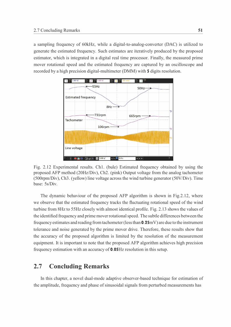
2.7 Concluding Remarks 51
a sampling frequency of 60kHz, while a digital-to-analog-converter (DAC) is utilized to
generate the estimated frequency. Such estimates are iteratively produced by the proposed
estimator, which is integrated in a digital real time processor. Finally, the measured prime
mover rotational speed and the estimated frequency are captured by an oscilloscope and
recorded by a high precision digital-multimeter (DMM) with 5 digits resolution.
Fig. 2.12 Experimental results. Ch1. (bule) Estimated frequency obtained by using the
proposed AFP method (20Hz/Div), Ch2. (pink) Output voltage from the analog tachometer
(500rpm/Div), Ch3. (yellow) line voltage across the wind turbine generator (50V/Div). Time
base: 5s/Div.
The dynamic behaviour of the proposed AFP algorithm is shown in Fig.2.12, where
we observe that the estimated frequency tracks the fluctuating rotational speed of the wind
turbine from 8Hz to 55Hz closely with almost identical profile. Fig. 2.13 shows the values of
the identified frequency and prime mover rotational speed. The subtle differences between the
frequency estimates and reading from tachometer (less than 0.25mV) are due to the instrument
tolerance and noise generated by the prime mover drive. Therefore, these results show that
the accuracy of the proposed algorithm is limited by the resolution of the measurement
equipment. It is important to note that the proposed AFP algorithm achieves high precision
frequency estimation with an accuracy of 0.05Hz resolution in this setup.
2.7 Concluding Remarks
In this chapter, a novel dual-mode adaptive observer-based technique for estimation of
the amplitude, frequency and phase of sinusoidal signals from perturbed measurements has

52 ADAPTIVE OBSERVER APPROACH: THE SINGLE SINUSOIDAL CASE
Fig. 2.13 Comparison of the estimated frequency obtained by using the proposed AFP method
and measured prime mover rotational speed.
been presented. The estimator embeds a switching criterion that disables the adaptation in
real-time under poor excitation conditions, thereby the behavior of the estimator in “dis-
excited” time interval is characterized. The ISS analysis is carried out to enhance not only
the robustness properties, but also the roles and the impacts of the adaptive parameters. This
chapter also offers a comprehensive investigation on the influence of different types of per-
turbations, including structured, unstructured and harmonic disturbances. More specifically,
the structured disturbances are modeled as a time-polynomial so as to represent bias and
drift phenomena typically present in applications, whereas the unstructured disturbances
are modeled as bounded noise signals. Harmonic disturbances are addressed through a
fundamental frequency identification problem, where the harmonics are treated as a part of
the generic periodic signal. Extensive simulations and real experiments have been carried
out to show the effectiveness of the proposed adaptive algorithm.
Chapter 3
ADAPTIVE OBSERVER APPROACH: THE
MULTI-SINUSOIDAL CASE
3.1 Introduction
In chapter 2, we presented an AO method for single (fundamental) frequency estimation
that is one of the basic issue arising in numerous practical applications. Nevertheless,
particular applications require online frequency estimates of harmonics and inter-harmonics.
In this respect, various types of methods emerge in the recent literature, such as [29, 55, 75,
76], which stem from the PLL and ANF concepts. As a consequence, only local stability
can be guaranteed in the most cases because of the averaging tools used for analysis. On the
contrary, the AO techniques [17, 46, 80, 100, 111] relying on a system model parametrized
by the coefficients of the characteristic polynomial, usually ensure global or semi-global
stability. The main drawback of the AO methods is the indirect frequency estimation
(computed as the zeros of the characteristic polynomial) which might result in an excessive
on-line computational burden.
In this chapter, the AO method discussed in Chapter 2 is extended to a solution for multi-
sinusoidal signals by proper model augmentation. In spirit of the initial results presented
in [22], the presented method deals with a direct adaptation mechanism for the squares of
the frequencies with semi-global stability guarantees. In contrast with [22] that is equipped
by a scalar switching signal globally regulating the adaptation of the frequency parameters,
the new estimator adopts a n dimensional excitation-based switching logic. Thanks to the
suitable matrix decomposition techniques, this novel switching criterion enables the update
of a parameter when the signal is sufficiently informative in that direction, thus enhancing the
practical implementation and avoiding unnecessarily disabled adaptation in the scenario that

54 ADAPTIVE OBSERVER APPROACH: THE MULTI-SINUSOIDAL CASE
0
i
only parts of the directions fulfill the excitation condition (e.g. over-parametrization). The
stability analysis proves the existence of a tuning parameter setting for which the estimator’s
dynamics are ISS with respect to bounded measurement disturbance.
The chapter is organized as follows: Section 3.2 is devoted to the formulation of the AFP
problem in the multi-frequency scenario. In particular, the nominal linear multi-sinusoidal
oscillator is transformed into an observable system with state-affine linear parametrization,
in which the parameter-affine term depends on the unknown frequencies. In Section 3.3, the
design of the adaptive observer-based estimator is treated. The embedded excitation-based
switching dynamics permit the analysis in case of poor excitement by freezing the estimates
under certain circumstances. Then, the stability of the presented approach is dealt with in
Section 3.4 by ISS concepts. Section 3.5 gives an example of the discretized algorithm for
digital implementation. Finally, in Section 3.6, simulations and practical experiments are
carried out to evaluate the behavior of the algorithm.
3.2 Problem formulation and preliminaries
Consider the following perturbed multi-sinusoidal signal:
n
v(t) = b + ai sin(ϕi(t)) + d(t) , i=1
(3.1) ϕ i(t) = ωi
with ϕi(0) = ϕi0 , where b is an unknown constant bias, the amplitudes of the sinusoids verify
the inequality ai ≥ 0, ∀i ∈ 1, . . . , n, ϕi0 is the unknown initial phase of each sinusoid,
while the term d(t) and the frequencies comply with Assumption 1 and 2 (see page 19)
respectively. Now, let us denote by y(t) the noise-free signal
n
y(t) = b + ai sin(ωit + ϕi ) (3.2) i=1
which is assumed to be generated by the following observable autonomous marginally-stable
dynamical system:
n
x (t) = Axx(t) + Aix(t)θ∗, x(0) = x0
(3.3)
y(t) = Cxx(t)
i=1

∗
i
c
0 c
3.2 Problem formulation and preliminaries 55
with x(t) /'. [x1(t) · · · x2n+1(t)]⊤ ∈ R2n+1 and where x0 represents the unknown initial
condition which leads the output to match the stationary sinusoidal behavior since the very beginning. The new parametrization θ∗, . . . , θ∗ used in (3.3) is related to the original
1 n
frequency parameters by the relationships
θi = αi + Ωi, ∀i ∈ 1, · · · , n, (3.4)
with Ωi = ω2, ∀i ∈ 1, · · · , n and where α1, α2, · · · , αn are non-zero constants that are
designed with the only requirements to satisfy αi = αj for i = j. The matrices of the linear
multi-oscillator (3.3) are given by
J1 02×2 · · · 02×2 0
⊤
1 02×2 J2
. . . 0
2×2
⊤ 2
Ax = .. . . . . . . ..
, C⊤ ..
. . .
. . x =
. , . . . . . . J 0
⊤ 02×2 n cn
0 · · · · · · 0 0 1
where 0r×s represents a r × s zero matrix, for generic indexes r and s
0 1
l
Ji =
αi 0 , ci =
I 1 0
1 .
Moreover, each Ai in (3.3) is a square matrix having the (2i, 2i − 1)th entry equal to −1.
Letting
A1 and A2 for instance are given by:
J0 =
0 0 l
−1 0
J0 02
l (2n 1)
02
2 02× 2 02× (2n
−3)
A1 = × −
, A2 = 02×2 J0 02×(2n−3) .
0(2n−1)×2 0(2n−1)×(2n−1)
0(2n−3)×2 0(2n−3)×2
0(2n−3)×(2n−3)
Thanks to (3.3), the noisy signal v(t) can be generated by the observable system
( x (t) = Axx(t) + Gx(x(t))θ∗, x(0) = x0
v(t) = Cxx(t) + d(t)
(3.5)
×
56 ADAPTIVE OBSERVER APPROACH: THE MULTI-SINUSOIDAL CASE
1 n
i 2i−1 2i
i 2i−1 2i
in which
Gx(x(t)) = I
G
(x(t)) · · · Gxi
(x(t)) · · · Gxn (x(t))
1 , (3.6)
Gxi (x(t)) = [01×(2i−1) x2i−1(t) 01×(2n+1−2i)]⊤, ∀i = 1, 2, · · · , n , (3.7)
and θ∗ ∈ Rn denotes the true parameter vector [θ∗ · · · θ∗ ]
⊤. According to Assumption 2,
there exists a known positive constant θ∗, such that |θ∗| ≤ θ
∗ . More specifically, in the
remaining parts of this chapter we consider θ∗ ∈ Θ∗, where Θ∗ ⊂ Rn is a hypersphere of
radius θ∗. It is important to stress that the constraint on θ∗ is instrumental for proving the
stability of the parameter adaptation law introduced in the next section, but is not needed in
the actual implementation of the algorithm.
It is clear from (3.6) and (3.7) that the elements of Gx(·) are globally Lipschitz continuous
functions due to the linearity of Gx(·). Moreover, the true state x(t) is norm-bounded for any
initial condition, i.e. |x(t)| ≤ x, ∀t ∈ R≥0. Both the Lipschitz condition on Gx(·) and the
bound x allow to establish the following further bound
∥Gx(x(t))∥ ≤ x, ∀t ∈ R≥0 .
Now, assuming that the estimates x(t) and θ(t) are available, then the full AFP estimates
are obtained by
Ω i(t) = max0, θi(t) − αi,
ωi(t) =
I
max0, θi(t) − αi, (3.8)
and
ai(t) =
/(Ω (t)x (t)2 + x (t)2
\ /Ω
i(t), (3.9)
ϕi(t) = ∠ (x2i(t) + ωi(t) x2i−1(t)) , i = 1, 2, · · · , n. (3.10)
In addition, the estimates of the offset is obtained directly by b = x2n+1. Note that the
possible singularity issue Ω i(t) = 0 affecting (3.9) is addressed by the following adaptive
amplitude estimators (3.11) in spirit of the previous treatment reported in Section 2.3 on the
estimation of a single sinusoidal signal:
a i(t) = −µaωi(t) ωi(t)ai(t) −
/ (Ω (t)x (t)2 + x (t)2
\
, (3.11) ai(t) = max0, ai(t)
x1

3.3 Filtered-augmentation-based adaptive observer 57
f
× ×
where ai(0) = ai(0) = 0, µa ∈ R>0 is an adjustable gain subject to the trade-off between
accuracy and convergence speed (see Fig. 2.4).
3.3 Filtered-augmentation-based adaptive observer
Recall the biased multi-oscillator (3.5), in which n unknown frequencies are embedded.
In order to address the frequency estimation task by means of an adaptive observer approach
(see [84] for a special case), let us first augment the dynamics of the observed system with a
synthetic low-pass filter driven by the noisy measurement:
vf (t) = Af vf (t) + Bf v(t) , (3.12)
where Af and Bf are set by the designer such that Af is Hurwitz and the pair (Af , Bf )
is controllable. vf (t) ∈ Rnf denotes the accessible state vector and with arbitrary initial
condition vf0 , such that the dimension nf of the augmented dynamics verifies nf = n − 1.
For the sake of the forthcoming analysis, it is convenient to split the filtered output into
two components:
vf (t) /'. yf (t) + df (t) ,
where yf (t) and df (t) can be thought as produced by two virtual filters, driven by the
unperturbed output and by the measurement disturbance, respectively:
yf (t) = Af yf (t) + Bf y(t), df (t) = Af df (t) + Bf d(t). (3.13)
Consequently, in view of (3.5), (3.13), the overall augmented system dynamics with the
extended perturbed output measurement equation can be written as follows:
z(t) = Azz(t) + Gz (z(t))θ
η(t) = Czz(t) η(t) = η(t) + dη (t)
, (3.14)
with z(0) = z0 ∈ Rnz , nz = 2n + 1 + nf = 3n, and z(t) /'. [x⊤(t) y⊤(t)]⊤, z0 /'. [x⊤(t) y⊤ ]⊤, η(t) /'. [v(t) v⊤(t)]⊤, dη (t) /'. [d(t) d⊤(t)]⊤,
0 f0 Az /'.
f
Ax 0(2n+1) (n
−1)
l
, Cz /'.
f
Cx 01 (n
l
−1) ,
BeCx Af 0(n−1)×(2n+1) I(n−1)
∗

58 ADAPTIVE OBSERVER APPROACH: THE MULTI-SINUSOIDAL CASE
θ
×
and
Gz (z(t)) /'.
Gx(Tzxz(t))
l
, 0(n−1)×n
with the transformation matrix given by Tzx /'. [I2n+1 0(2n+1)×(n−1)]. It is worth noting
that Gz (z(t)) is also Lipschitz, with unitary Lipschitz constant as Gx(x(t)), and can be
norm-bounded by x. Moreover, the assumed norm-bound d on the output noise implies the
existence of dη such that dη > 0 : |dη (t)| ≤ dη, ∀t ∈ R≥0 .
Now, we introduce the structure of the adaptive observer for obtaining estimates of the
unknown parameter vector θ∗, and in turn frequency estimates Ω i, i = 1, · · · , n. Besides the
measured output filter (3.12), the architecture of the estimator also includes three dynamic
components (3.15), (3.16) and (3.18), which are described below:
1) Augmented state estimator:
z(t) = (Az − LCz )z(t) + Lη(t) + Gz (z(t))θ(t) + Ξ(t) ˆ (t) (3.15)
with z(0) = z0 and where Ξ(t) is defined in (3.17). The gain matrix L is given by
L /'.
Lx 0(2n+1) (n
l −1)
0(n−1)×1 0(n−1)×(n−1)
where Lx is a suitable gain matrix such that (Ax − LxCx) is Hurwitz. Additional constraints
on the poles’ selection are discussed in Theorem 3.4.1.
2) Parameter-affine state-dependent filters:
Let Gz1 (z(t)), · · · , Gzn (z(t)) be the columns of Gz (z(t)), that is
Gz (z(t)) = I G (z(t)) · · · Gzi (z(t)) · · · Gzn
(z(t)) 1
.
Then, we introduce a set of auxiliary signal ξi(t), i = 1, · · · , n, whose dynamics obeys the
following differential equations driven by the available (estimated) counterpart of Gz (z(t)):
ξi(t) = (Az − LCz )ξi(t) + Gzi (z(t)), ∀i = 1, · · · , n , (3.16)
with ξi(0) = 0nz×1 . By collecting all the filters’ states, we get the auxiliary signal matrix
Ξ(t) = [ξ1(t) · · · ξi(t) · · · ξn(t)] , (3.17)
used in (3.15).
3) Frequency adaptation unit:
z1

3.3 Filtered-augmentation-based adaptive observer 59
θpre
θpre
Ψ
z
Herein, an projection operator P is utilized to confine the estimated parameter θ(t) to the
predefined convex region Θ∗
˙ θ(t) = P
I ˙ 1
θpre(Ψ(t), t) |≤θ∗
(3.18)
with θ(0) = θ0 set arbitrarily, and where ˆ is the unconstrained parameter’s derivative,
whose explicit expression is given in (3.21); Ψ(t) ∈ Rn×n represents a diagonal matrix
consisting of binary (1: on, 0: off) on-off switching signals which enable or disable the
adaptation of a specific parameter:
Ψ(t) /'. diag[ψ1(t), · · · , ψi(t), · · · , ψn(t)] . (3.19)
The adaptation-enabling signals ψi(t), ∀i = 1, 2, · · · , n will be specified later on. For the
sake of brevity, we write θpre(t) instead of θpre(Ψ(t), t), dropping the dependence of θpre on
Ψ(t) in the rest of the section. The parameters’ derivative projection operator in (3.18) is
defined as [52]:
Iˆ 1
θpre
θ(t)θ⊤(t) ˙ e P θpre(t)
|≤θ∗ /'. ˙ (t) − I(θ)
θ∗2 θpr (t) (3.20)
where I(θ) denotes the indicator function, defined as: (
1, if |θ(t)| = θ∗ and θ⊤(t) ˆ (t) > 0 , I(θ) /'.
0, otherwise .
Now, the unconstrained derivative is given by:
ˆ ˘ θpre(t) /'. −µUΨ(t) (Ψ(t)SΨ(t)) U⊤(t)UΞ(t)SΞ(t)U⊤(t)Ξ⊤(t)C⊤ (Cz z(t) − η(t)) ,
Ψ Ξ z
(3.21)
with UΨ, SΨ, UΞ, SΞ defined in the following. The matrices UΨ and SΨ are obtained by the
SVD of ΣΨ(Ξ(t)):
ΣΨ(Ξ(t)) /'. (Ξ⊤(t)Ξ(t) + ρ2I
)−
= UΨ(t)SΨ(t)U⊤(t)
Ξ⊤(t)C⊤Cz Ξ(t)
in which SΨ(t) is a diagonal matrix comprising all the eigenvalues of ΣΨ(Ξ(t)). Analogously,
UΞ and SΞ are obtained by the SVD of the matrix ΣΞ(Ξ) defined as:
ΣΞ(Ξ(t)) /'. Ξ⊤(t)C⊤Cz Ξ(t) = UΞ(t)SΞ(t)U⊤(t) . z Ξ
1
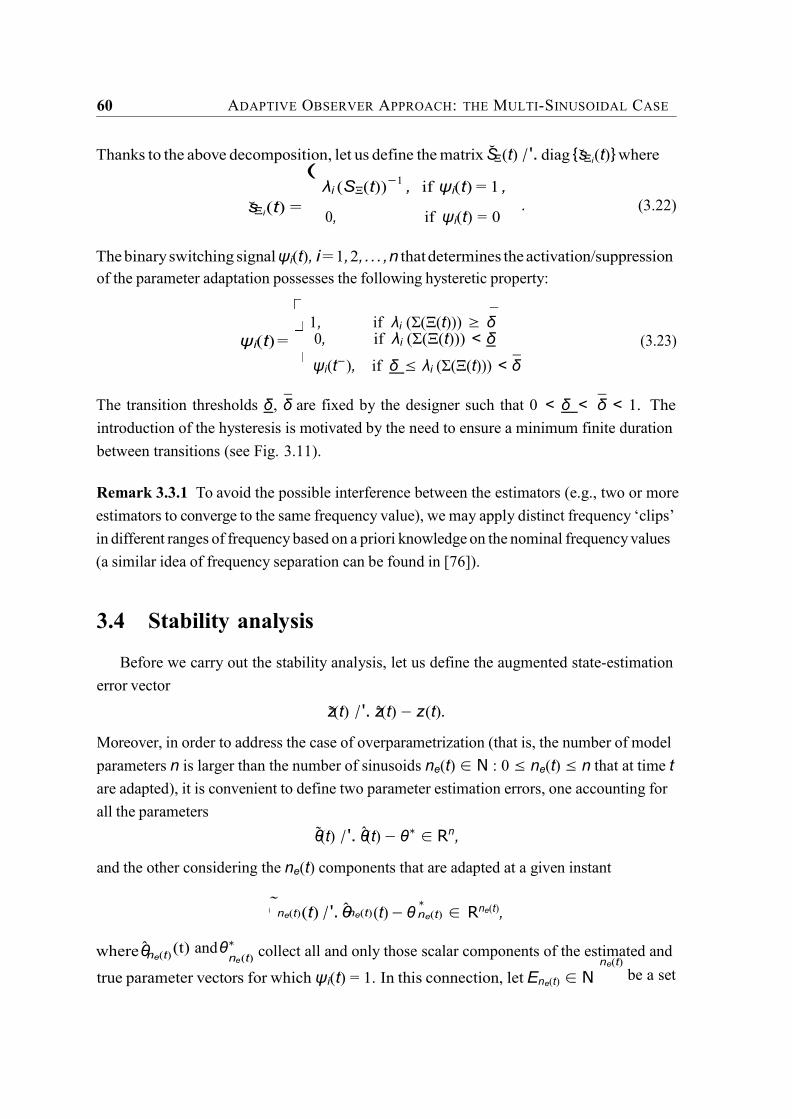
60 ADAPTIVE OBSERVER APPROACH: THE MULTI-SINUSOIDAL CASE
ne(t)
ne(t) n (t)
Thanks to the above decomposition, let us define the matrix SΞ(t) /'. diag sΞi (t) where (
λi (SΞ(t))−1
, if ψi(t) = 1 ,
sΞi (t) = 0, if ψi(t) = 0
. (3.22)
The binary switching signal ψi(t), i = 1, 2, . . . , n that determines the activation/suppression
of the parameter adaptation possesses the following hysteretic property:
¯
ψi(t) =
1, if λi (Σ(Ξ(t))) ≥ δ 0, if λi (Σ(Ξ(t))) < δ
ψi(t
−), if δ ≤ λi (Σ(Ξ(t))) < δ
(3.23)
The transition thresholds δ, δ are fixed by the designer such that 0 < δ < δ < 1. The
introduction of the hysteresis is motivated by the need to ensure a minimum finite duration
between transitions (see Fig. 3.11).
Remark 3.3.1 To avoid the possible interference between the estimators (e.g., two or more
estimators to converge to the same frequency value), we may apply distinct frequency ‘clips’
in different ranges of frequency based on a priori knowledge on the nominal frequency values
(a similar idea of frequency separation can be found in [76]).
3.4 Stability analysis
Before we carry out the stability analysis, let us define the augmented state-estimation
error vector
z(t) /'. z(t) − z(t).
Moreover, in order to address the case of overparametrization (that is, the number of model
parameters n is larger than the number of sinusoids ne(t) ∈ N : 0 ≤ ne(t) ≤ n that at time t
are adapted), it is convenient to define two parameter estimation errors, one accounting for
all the parameters
θ(t) /'. θ(t) − θ∗ ∈ Rn,
and the other considering the ne(t) components that are adapted at a given instant
˜ ne(t) (t) /'. θ
∗ ne(t) ∈ Rne(t),
where θ (t) and θ∗ e
collect all and only those scalar components of the estimated and ne(t)
true parameter vectors for which ψi(t) = 1. In this connection, let Ene(t) ∈ N be a set
θ (t) − θ

3.4 Stability analysis 61
∗
i=1
θi
containing the integer indexes of all and only those components for which the adaptation is
enabled at time t.
As said above, the case of overparametrization herein corresponds to a situation in which
the number of frequency parameters of the observer, n, is larger than ne(t), the number
of dominant sinusoids in terms of amplitude with unique frequency forming the measured
signal1 (more details of overparametrization in the context of adaptive control can be found
in [104]). In this case a minimal realization of the generator of the measured signals is a
multi-harmonic oscillator of order 2ne, composed by the collection of exactly ne unique
harmonic oscillators [37]. Accordingly, a non-minimal realization for such a signal generator
can be taken as the union of the said minimal multi-harmonic oscillator with an augmented
dynamics formed by (n − ne) harmonic oscillators with null-states and arbitrary frequencies.
The possibility to assign arbitrarily the frequency of the augmented null-amplitude multi-
oscillator is the key for proving the stability in this context. For the sake of the further
discussion, without loss of generality, let us take the frequency parameters of the augmented
dynamics equal to the present estimates produced by the filter for the components not adapted
due to poor excitation, achieved by
θi = θi(t), ∀i ∈ 1, 2, · · · , n\Ene(t), (3.24)
which implies θi(t) /'. θi(t) − θ∗ = 0, ∀i ∈ 1, 2, · · · , n\En (t). (3.25)
i e
For the sake of the further discussion let us also define the linear time-varying combination
of state and parameter vectors ζ(t) /'. ),n
evolves according to the differential equation:
ξi(t)θi(t) − z(t), The state-estimation error
n
z(t) =(Az − LCz )z(t) + Ldη (t) + Gz (z(t))θ(t) + Gz (z(t))θ∗ + ξi(t) ˆ
(t)
=(Az − LCz )z(t) + Ldη (t) + Gz (z(t))θ∗ +
i=1
Gz (z(t))θi(t) + Ξ(t) ˆ(t) ,
i
i∈Ene(t)
θ
(3.26)
where Gz (z(t)) /'. Gz (z(t)) − Gz (z(t)) . Meanwhile, the auxiliary variable ζ(t) evolves
according to
ζ˙(t) =
i∈Ene(t)
ξi(t)θi(t) + Ξ(t)θ˙(t) − z(t) , (3.27)
1The residual sinusoidal signals not accounted for by the adaptation are masked and implicitly treated as a
disturbance.

62 ADAPTIVE OBSERVER APPROACH: THE MULTI-SINUSOIDAL CASE
i
which, after some algebra, leads to
ζ˙(t) =
i∈Ene(t)
((Az − LCz )ξi(t)θi(t) + Gz (z(t))θi(t)
\ + Ξ(t)θ
˙(t) − (Az − LCz )z(t)
−Gz (z(t))θ(t) − Ldη (t)−Gz (z(t))θ(t)−Gz (z(t))θ∗−Ξ(t)θ
˙(t)
= (Az − LCz )ζ(t) − Ldη (t) − Gz (z(t))θ∗ .
(3.28)
In Fig. 3.1, we draw the overall excitation-based switching scheme, which is instrumental
for the forthcoming analysis. In principle, the adaptation is deemed activated as long as
ne = 0, which means at least one component is updating. An active identification interval
always starts from a transition to active identification time-interval, and ends up with a
transition to dis-excitation time-interval, while the dis-excitation interval is the opposite.
More specifically, let ke(t) be a counter for the transitions to excitation, described by the
Fig. 3.1 Scheme of the excitation-based switching scheme for enabling/disabling the param-
eter adaptation. The transitions to dis-excitation (a) and to active identification phases (b)
have been highlighted.

3.4 Stability analysis 63
1
1 ne
jump dynamics given below: (
ke(t−) + 1, if En (t−) = ∅ and En (t) = ∅ ,
ke(t) = e e
ke(t−), if Ene (t−) = ∅ and Ene (t) = ∅ .
Analogously, let k1→0(t) be a counter with respect to the transition from excitation to dis-
excitation: ( kd(t−) + 1, if En (t
−) = ∅ and En (t) = ∅ , kd(t) =
e e
kd(t−), if Ene (t−) = ∅ and Ene (t) = ∅ .
Moreover, let td(k) and te(k) denote the transition time-instants:
te(k) /'. inf(t ≥ 0 : ke(t) = k) , td(k) /'. inf(t ≥ 0 : kd(t) = k) .
Without loss of generality and taking into account that the system starts from zero-excitement,
then
te(k) > td(k), ∀k ∈ Z>0 .
and the counters are initialised by ke(0) = 0, kd(0) = 1 . Hence, the integer k always
identifies a two-phase time-window made of a dis-excitation interval followed by an active
estimation interval (see Fig. 3.1).
Since (Az − LCz ) is Hurwitz, for any positive definite matrix Q, there exist a positive
definite matrix P that solves the linear Lyapunov equation
(Az − LCz )⊤P + P (Az − LCz ) = −2Q .
In the following, we analyze the behaviour of the adaptive observer in two situations by a
Lyapunov candidate that accounts for all the parameters:
where g ∈ R>0.
V (t) /'. 2
(z⊤(t)P z(t) + θ⊤(t)θ(t) + gζ⊤(t)P ζ(t)
) , (3.29)
i) Active adaptation interval of finite duration, i.e. in which ne(t) ≥ 1 = ne, ∀t ∈
[te(k), td(k + 1)] (we omit the time-dependence of ne assuming that for the whole interval it
remains constant). In this case the set Ene (t) is non-empty, V (t) defined in (3.29) shrinks to
the following positive definite function, considering the sole components actively adapted:
Vne (t) /'. 2
(z⊤(t)P z(t) + θ⊤ (t)θne (t) + gζ⊤(t)P ζ(t)
) . (3.30)

64 ADAPTIVE OBSERVER APPROACH: THE MULTI-SINUSOIDAL CASE
θpre
θpre
θpre
θpre
In this interval, we prove that Vne is an ISS-Lyapunov function for the system comprising
all states and only the parameters undergoing adaptation, that will converge to the true
values. The present scenario comprises, besides the overparametrization case, also the
full-parametrization case, which yields to the ISS of the whole dynamics.
ii) Total dis-excitation, i.e., none of the parameters is adapted due to poor excitation. In
this scenario the set Ene(t) is empty. In this case we show that the overall function (3.29)
remains bounded.
After that, the Lyapunov analysis in these two scenarios are linked properly and we are
able to prove that the alternate occurrence of active identification phases and poorly excited
phases yields to convergence, provided that the active identification phases have a sufficient
duration. To simplify the analysis, we will consider that the number of adapted sinusoidsne
is fixed (i.e., Ene(t) is an invariant set) within a whole excitation/dis-excitation interval (see
Fig. 3.1), that is the set Ene(t) may be either the empty set 0 during the dis-excitation phase,
either a set Ene = ∅ for an arbitrary active adaptation interval. Note that this assumption
does not limit the applicability of the adaptive observer to this very special case, being it
just a technicality needed to render the problem tractable in a simple analytical way (an
active adaptation phase with time-varying ne(t) can be regarded as a combination of multiple
excited intervals).
3.4.1 Active adaptation interval of finite duration
Consider an arbitrary active identification phase te(k) ≤ t < td(k + 1) (see Fig. 3.1) and
let Ψne (t) be the binary matrix in this scenario with only ψi(t) = 1, ∀i ∈ Ene . The upcoming
analysis is carried out in order to exhibit the benefit of using the derivative projection on
the parameters’ estimates. Thanks to (3.20), in the presence of the projection I(θ) = 1 and
|θ(t)| = θ∗, we have
θ⊤(t) ˆ (t) = θ⊤(t) ˆ (t) − θ⊤(t) θ(t)θ⊤(t) ˆ
¯
(t)
θ θpre θ∗2 θpre
= θ⊤(t) ˆ 1
(t) − θ∗2
θ⊤(t)θ(t)θ⊤(t) ˆ (t) .
Owing to the convexity of the admissible set, it holds that θ⊤(t)θ(t) = (θ⊤(t) − θ∗⊤
\ θ(t) ≥
0 . Now, we recall the triggering condition of projection θ⊤(t) ˆ (t) > 0, which implies that
1
θ∗2 θ⊤(t)θ(t)θ⊤(t) ˆ (t) ≥ 0 .
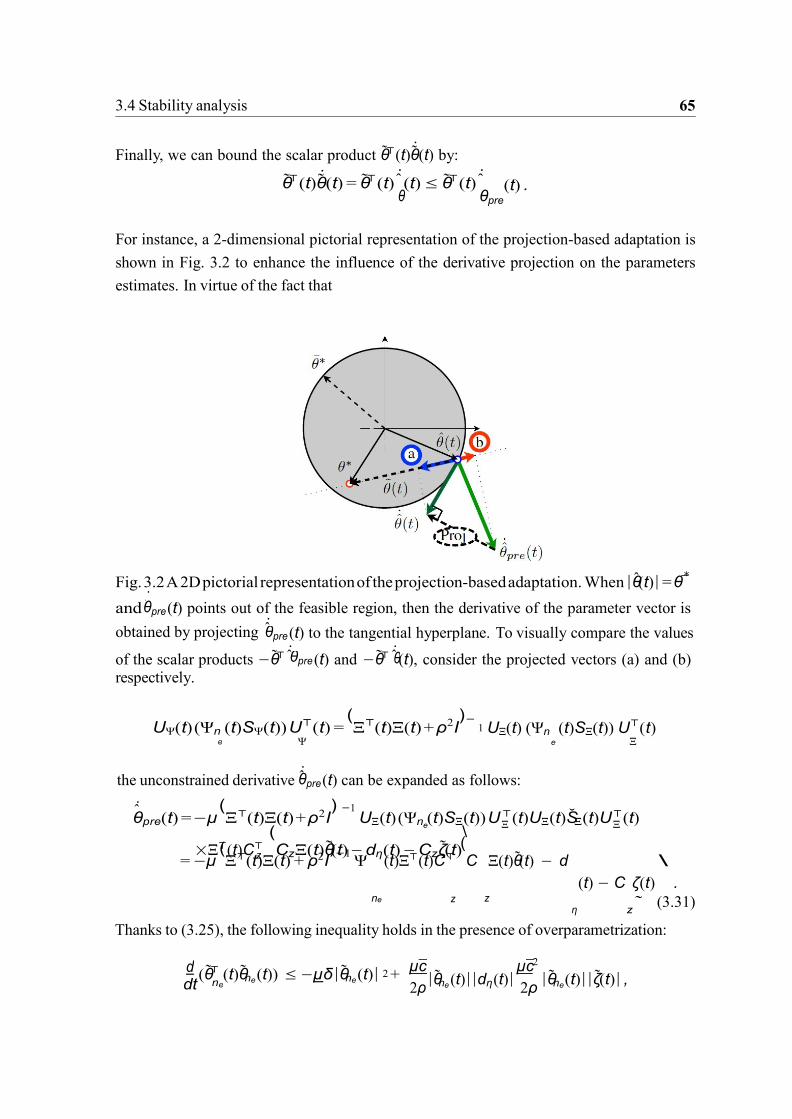
3.4 Stability analysis 65
and
θpre
θpre θ
θpre
z
ne
d 2
Finally, we can bound the scalar product θ⊤(t)θ˙(t) by:
θ⊤(t)θ˙(t) = θ⊤(t) ˆ (t) ≤ θ⊤(t) ˆ
(t) .
θ θpre
For instance, a 2-dimensional pictorial representation of the projection-based adaptation is
shown in Fig. 3.2 to enhance the influence of the derivative projection on the parameters
estimates. In virtue of the fact that
Fig. 3.2 A 2D pictorial representation of the projection-based adaptation. When |θ(t)| = θ∗
˙ θpre (t) points out of the feasible region, then the derivative of the parameter vector is
obtained by projecting ˆ (t) to the tangential hyperplane. To visually compare the values
of the scalar products −θ⊤ (t) and −θ⊤ ˙(t), consider the projected vectors (a) and (b) respectively.
UΨ(t) (Ψn (t)SΨ(t)) U⊤(t) = (Ξ⊤(t)Ξ(t) + ρ2I
)− UΞ(t) (Ψn (t)SΞ(t)) U⊤(t)
Ψ
the unconstrained derivative ˆ
ˆ
e Ξ
(t) can be expanded as follows:
−1 θpre(t) = −µ
(Ξ⊤(t)Ξ(t) + ρ2I
) UΞ(t) (Ψn (t)SΞ(t)) U⊤(t)UΞ(t)SΞ(t)U ⊤(t)
×Ξ⊤(t)C⊤
e Ξ Ξ (Cz Ξ(t)θ(t) − dη (t) − Cz ζ(t)
\
= −µ (Ξ⊤(t)Ξ(t) + ρ2I
)−1 Ψ (t)Ξ⊤(t)C⊤
(C Ξ(t)θ(t) − d \
(t) − C ζ(t) . ne z z
η z (3.31)
Thanks to (3.25), the following inequality holds in the presence of overparametrization:
dt (θ⊤ (t)θne (t)) ≤ −µδ|θne (t)| +
µc
2ρ |θne (t)||dη (t)|
µc2
2ρ |θne (t)||ζ(t)| ,
e
1
66 ADAPTIVE OBSERVER APPROACH: THE MULTI-SINUSOIDAL CASE
| ne || η | −
2
where c /'. ∥Cz ∥.
The following result can now be proven.
Theorem 3.4.1 (ISS of the dynamic estimator) If Assumption 2 holds, given the sinusoidal
signal y(t) defined in (3.2) and the perturbed measurement (3.1), then in an active adaptation
interval te(k) ≤ t < td(k + 1), there exist poles of (Ax − LxCx), µ ∈ R>0 and ρ ∈ R>0
such that Vne (t) is an ISS Lyapunov function with respect to any bounded disturbance dη and
in turn ISS w.r.t. bounded measurement disturbance |d(t)| ≤ d. Thus z(t) and θne (t) are ISS
w.r.t. d. D
Proof: In view of (3.24), we immediately have |θ(t)| = |θne |, which implies V (t) = Vne (t),
and makes it possible to study the time-derivative of Vne (t) in place of V (t):
1 ⊤ ˜ g ( ˜ ˜ ˜ ˜
Vne (t) = (z⊤(t)P z(t) + z
2 (t)P z(t)
) + θne (t)
⊤θne (t) + 2
ζ⊤(t)P ζ(t) + ζ⊤(t)P ζ(t)) .
(3.32)
By letting l /'. ∥L∥, q /'. λ(Q),
follows:
p /'. λ(P ), after some algebra, V (t) can be bounded as
2 ˜ 2 ˜ 2 ¯ 2 ˜
Vne (t) ≤ −q|z(t)| — gq|ζ(t)| — µδ|θne (t)| + pl|z(t)||dη (t)| + p|z(t)| |θ(t)|
+px|z(t)||θ(t)| + pθ∗|z(t)|2 + µpc2|z(t)|2 + µpc|z(t)||dη (t)| c +µ |θne (t)||dη (t)| + µ c
2 |θne (t)||ζ(t)| + gpl ζ(t)||dη (t)| + gpθ∗
|z(t)||ζ(t)| .
2ρ 2ρ | ne
In view of the inequality |θne (t)| = |θ(t)| ≤ 2θ∗ and by re-arranging the above inequality to
put in evidence the square monomial and the binomial terms, we get:
2 ¯∗ 2 ¯ gq ˜ 2
gq 2
Vne (t) ≤ −(q − µpc — 3pθ )|z(t)| + p(l + µc
)|z(t)||dη (t)| −
2 |ζ(t)| −
4 |ζ(t)|
gq
|
µδ ˜ 2 µδ ˜ 2
+gpθ∗|z(t)||ζ(t)| − 4
|ζ(t)| + gpl ζ(t)||dη (t)| − 2
|θne (t)| − 6
|θne (t)|
+px|z(t)||θne (t)| − c2
µδ 2
6 |θne (t)|
c + µ θ (t) d (t)
2ρ
µδ 2
6 |θne (t)|
+µ 2ρ
|θne (t)||ζ(t)| .
Now, we complete the squares, thus obtaining
(q − µpc2 − 3pθ∗) g (
¯ )2 3(px)2
l gq 3µc4
Vne (t) ≤ − 2
− q
p θ∗
− 2µδ |z(t)|2
− ( 2
− 8ρ2δ
)|ζ(t)|
2(¯ 2
l µδ ˜ 2 p l + µc
) 3µc2
g 2 2 2
− 2
|θne (t)| + 2(q − µpc2 3pθ∗)
+ 8ρ2δ
+ q
p l |dη (t)| .
2
2
−

3.4 Stability analysis 67
β
l
Finally, the following inequality can be established:
Vne (t) ≤ −β1
lVne (t) − γ1(dη )
l , (3.33)
where ((q − µpc2 − 3pθ∗)
g (¯ )2
3x2p µδ q
3µc4
β1 /'. 2 min 2p —
q p θ∗
,
2µδ 2 ,
2p −
8gρ2δp (3.34)
and 1 p2
(l + µc
)2
3µc2
g2 2 2
γ1(r)/'. 1 2(q − µpc2
3pθ∗) +
8ρ2δ +
q p l
r , ∀r ∈ R≥0 . (3.35)
Hence, the proof is concluded if
β1 > 0. (3.36)
In view of (3.36), all the components involved in (3.34) should be positive, wherein µδ/2 > 0
can be immediately verified by choosing a positive µ. Now, we set the excitation threshold
δ and the Q matrix arbitrarily, determining q. Then, assume the poles of (Ax − LxCx) are
placed such that p is sufficient small. Letting p ≤ µ, we determine a sufficient condition to
ensure the positiveness of the first term in (3.34):
(q − µ2c2 − 3µθ∗) (¯
)2
2 g
2 − µ
q θ∗
3x2
− µ 2δ
> 0. (3.37)
Being the Lyapunov parameter g > 0 arbitrary, let us fix g = 1 for simplicity. At this point,
with any fixed regularization parameter ρ ∈ R>0 (we do not pose limits on ρ now) we can
always determine a sufficiently small value of µ for which the inequality holds true. Next, by
suitably allocating the poles, we compute the output-injection gain L that realizes the needed
p. Finally, to render β1 strict-positive, we choose a sufficient large ρ such that
q 3µc4
2p −
8gpρ2δ > 0 .
thus ending the proof. •
Remark 3.4.1 (Parameter tuning) To avoid the increase of the worst-case sensitivity to
bounded noises, instead of excessively reducing the value of p that leads high-gain output
injection through L, and high values of l and γ1 correspondingly, we can set p = µ and
increase the regularization parameter ρ.
−
−

68 ADAPTIVE OBSERVER APPROACH: THE MULTI-SINUSOIDAL CASE
i=1
2
2 4
˜
2 4
˜
2
3.4.2 Total dis-excitation phase
Clearly, it is important to show that the estimation error remains bounded also during the
time-intervals in which no excitation is present (e.g., td(k) ≤ t < te(k) as illustrated in Fig.
3.1). This is carried out in the following result.
Lemma 3.4.1 (Boundedness in dis-excitation phase) Under the same assumptions of The-
orem 3.4.1, consider an arbitrary dis-excitation interval td(k) ≤ t < te(k) in which
Ene (t) = ∅. Then, under suitably chosen µ ∈ R>0, ρ ∈ R>0 and the poles of (Ax − LxCx),
V (t) is an ISS Lyapunov function w.r.t. d(t) (where |d(t)| ≤ d) and w.r.t. V (td(k)). D
Proof: In the considered dis-excitation scenario, the estimation is totally unexcited in all
directions, i.e. ),n
ψi(t) = 0, ∀t ≥ td(k) > 0, thus yielding θ˙(t) = 0n ×1, and θ(t) = θ(t−).
In this respect, the time-derivative of the Lyapunov function V (t) satisfies
V (t) ≤ −(q − 3pθ∗)|z(t)|2 + pl|z(t)||dη (t)| − gq
|ζ(t)|2 −
gq
|ζ(t)|2 + gpθ∗|z(t)||ζ(t)|
gq ˜ 2 ˜
| −
4 |ζ(t)|
+ gpl ζ(t)||dη (t)| + px|z(t)||θ(t)| .
Applying the inequality |θ(td(k))|2 ≤ 2V (td(t)), ∀t ≥ td(k), we have:
V (t) ≤ −(q − 3pθ∗)|z(t)|2 + pl|z(t)||dη (t)| − gq
|ζ(t)|2 −
gq
|ζ(t)|2 + gpθ∗|z(t)||ζ(t)| gq
˜ 2 ˜ 2 ˜
| −
4 |ζ(t)|
+ gpl ζ(t)||dη (t)| − |θ(t)| + 2V (td(k)) + px|z(t)||θ(t)| .
By completing squares, we obtain the following upper bound for V (t):
(q −3pθ∗) g (¯
)2 3(px)2 l
5 gq
V (t) ≤− 2
− q
p θ∗ − 2 |z(t)|2
− 6 |θ(t)| −
2 |ζ(t)|
+ 2V (td(k))
p2l2
2(q − 3pθ∗)
+ g
p2l2
q
|dη (t)|2
and hence, after some algebra, it follows that
V (t) ≤ −β0
(V (t) − L0V (td(k)) − γ0(dη (t))
) (3.38)
where L0 /'. 2/β0,
β0 /'. 2 min
((q − 3pθ∗)
2p
g
— q
p
(θ∗)2
−
3px2 ,
2
5 q
, 6 2p
2
+
l

3.4 Stability analysis 69
β
1
d
l
and 1 p2l2 g 2 2 2
γ0(r) /'. 0 2(q 3pθ∗)
+ q
p l r , ∀r ∈ R≥0 .
The positiveness of β0 can be justified by following the same steps taken in Section 3.4.1. It
is easy to show that β0 > 0 is ensured through a suitable design of µ and ρ, thus concluding
the proof. •
3.4.3 Robustness Under Alternate Switching
At this stage, the stability of the adaptive observer under alternate switching is charac-
terized by linking the results obtained for the two excitation phases. Thanks to the Bellman
Gronwall lemma, we are able to prove that the alternate occurrence of active identifica-
tion phases and poorly excited phases may yield to convergence provided that the active
identification phases have a sufficient duration.
Theorem 3.4.2 Under the same assumptions of Theorem 3.4.1, consider the adaptive ob-
server (3.12), (3.15)- (3.18) equipped with the excitation-based switching strategy defined in
(3.42). Then, the discrete dynamics induced by sampling the adaptive observer in correspon-
dence of the switching transitions has the asymptotic ISS property if the excitation phases
last longer than β−1 ln(L0). D
Proof: By the B-G Lemma, the value of the Lyapunov function (3.38) within the dis-excitation
intervals can be bounded as follows:
V (t) ≤ V (td(k)) + (1−e−β0(t−td)
) (L0V (t−(k))+γ0(dη )−V (td(k))
) ,
∀t ∈ [td(k), te(k)), ∀k ∈ Z>0 .
Instead, during the excitation phases, the Lyapunov function (3.33) can be bounded as
V (t) ≤ V (te(k)) + (1 − e−β1(t−te(k))
) (γ1(dη ) − V (te(k))
) ,
∀t ∈ [te(k), td(k + 1)), ∀k ∈ Z>0 .
In order to link the two modes of behaviour, let us denote by Vk = V (td(k)) the value of the
Lyapunov function sampled at the k-th transition to dis-excitement, occurring at time td(k)
(or equivalently, at the end of the (k − 1)-th active identification phase).
Due to the poor excitation during the interval [td(k), te(k)), at the transition time te(k)
we can establish the (possibly conservative) bound
V (te(k)) ≤ L0Vk + γ0(dη ) .
−

70 ADAPTIVE OBSERVER APPROACH: THE MULTI-SINUSOIDAL CASE
0
β−1
t
Such a bound holds for any duration the disexcitation phase. For any subsequent active
identification time t = te(k) + ∆t with ∆t < td(k + 1) − te(k), we get the inequality:
V (t) ≤V (te(k))+(1 − e−β1(t−te(k))
) (γ1(dη )−V (te(k))
)
=γ1(dη )−e−β1(t−te(k))γ1(dη )+e−β1(t−te(k))V (te(k))
≤ γ1(dη ) − e−β1(t−te(k))γ1(dη ) + e−β1(t−te(k)) (γ0(dη ) + L0Vk
)
= γ1(dη ) + e−β1∆t (γ0(dη ) − γ1(dη ) + L0Vk
) .
Now, let us arbitrarily set 0 < κ < 1 and let ∆Te = −β−1 ln (L−1κ
). If the active
1 0
identification phase is long enough to verify the inequality td(k + 1) − te(k) > ∆Te, then we
can guarantee the following difference bound on the discrete (sampled) Lyapunov function
sequence: κ
Vk+1 ≤ γ1(dη ) + 0
(γ0(dη ) − γ1(dη )
) + κVk
which can be rewritten in the following compact form:
Vk+1 − Vk ≤ −(1 − κ)Vk + γ(dη ) ,
where γ(s) = γ1(s) + κL−1 (γ0(s) − γ1(s)) , ∀s ≥ 0.
We can conclude that Vk is a discrete ISS Lyapunov function for the sampled sequence,
with samples taken at the end of the excitation phases assumed always to last longer than
1 ln(L0).
Now, we recover the ISS properties for the continuous-time system by studying the inter-
sampling behaviour of V (t). Let k(t), ∀t > 0 denote the index of the current time-window:
k(t) = k : t ∈ ltd(k), td(k + 1)
) and consider two positive constants ∆t1, ∆t2, such that
∆t1 ≤ te(k) − td(k), ∆t2 ≤ td(k + 1) − te(k). Between two samples, the Lyapunov function
is bounded by:
V (t) ≤ max ∆t1∈R≥0
Vk(t) +
(1 − e−β0∆t1
) (L0Vk(t) + γ0(dη ) − Vk(t)
)
+ max γ1(dη ) − e−β1∆t2
(γ1(dη ) − γ0(dη ) − L0Vk(t)
)
∆t2∈R≥0
≤ l(1 + L0)Vk(t) + γ0(dη )
l +
lγ1(dη ) + γ0(dη ) + L0Vk(t)
l
= (1 + 2L0)Vk(t) + γ1(dη ) + 2γ0(dη ) .
(3.39)
If we let k(t) −−−→ →∞
∞ (i.e., an infinite number of active identification phases occurs
asymptotically or a single excitation phase lasts indefinitely), then the estimation error in
the inter-sampling times converges to a region whose radius depends only on the assumed
disturbance bound. •
L

β−1
1
1
3.5 Digital implementation of the proposed method 71
Remark 3.4.2 It is worth noting that the thresholds δ and δ play important roles in the
behavior of the estimator under alternate switches. Because of the hysteretic property, the
values of δ and δ have to be properly set to avoid the excitation signals of the adapted
frequencies being confined in the transient interval (i.e., [δ, δ]). Suitable choices can be
found off-line by a priori information of the inputs.
Remark 3.4.3 In practical applications, in order to the improve the speed of convergence, a
robust provision can be adopted consisting in re-initializing the parameter-vector with the
value estimated by a previous sufficiently long identification phase (i.e. td(k + 1) − te(k) ≥
1 ln(L0)) after any insufficiently long excitation interval. In this respect, let k∗ be a counter
for the sole active identification phases lasting more than the minimal duration β−1 ln(L0)
and consider Vk∗ = V (td(k∗)). In this case, Vk∗ is a discrete ISS Lyapunov function for the
sampled adaptive observer, with samples collected at the end of the sole excitation phases
lasting longer than β−1 ln(L0).
3.5 Digital implementation of the proposed method
In this section, we show a counterpart of this switched algorithm in the discrete-time
domain to enhance the applicability. Similar to the one presented in Section 2.5, the first
step consists in selecting a set of parameters Af , Bf , α1, α2, µ, ρ, µA, δ, δ; after that, Euler
method is employed with a sampling period is Ts, thus resulting in a discretized algorithm
given as follows, provided a measurement v(k), k = 1, 2, · · ·
vf (k) = vf (k − 1) + Ts (Af vf (k − 1) + Bf v(k)) , (3.40a)
z(k) = z(k − 1) + Ts
((Az − LCz )z(k − 1) + Lη(k) + Gz (z(k − 1))θ(k − 1)
\ (3.40b)
+ Ξ(k − 1)(θ(k − 1) − θ(k − 2)) ,
(3.40c)
Ξ(k) = Ξ(k − 1) + Ts ((Az − LCz )Ξ(k − 1) + Gz (z(k))) , (3.40d)
θpre(k) = θpre(k − 1) (3.40e)
+ Ts
(−µUΨ(k) (Ψ(k)SΨ(k)) U⊤(k)UΞ(k)SΞ(k)U ⊤(k)Ξ⊤(k)C⊤ (Cz z(k) − η(k))
\ ,
Ψ Ξ z
(3.40f)
θ(k) = θ(k − 1) + θpre(k) − θpre(k − 1) − I(θ) θ(k − 1)θ⊤(k − 1)
θ∗2 \
(3.40g)
(ˆ ˆ
× θpre(k) − θpre(k − 1) , (3.40h)

72 ADAPTIVE OBSERVER APPROACH: THE MULTI-SINUSOIDAL CASE
f
θpre
i 2i−1 2i
where η(k) /'. [v(k) v⊤(k)]⊤, UΨ(k), SΨ(k), UΞ(k), SΞ(k) are obtained by the SVD of
ΣΨ(Ξ(k)) and ΣΞ(Ξ(k)) at the corresponding sampling instant, that is
ΣΨ(Ξ(k)) = (Ξ⊤(k)Ξ(k) + ρ2I
)− Ξ⊤(k)C⊤Cz Ξ(k) = UΨ(k)SΨ(k)U⊤(k)
z Ψ
ΣΞ(Ξ(k)) /'. Ξ⊤(k)C⊤Cz Ξ(k) = UΞ(k)SΞ(k)U⊤(k) .
z Ξ
Furthermore, in view of (3.22), we have SΞ(k) = diag sΞi (k) where (
λi (SΞ(k))−1
, if ψi(k) = 1 ,
sΞi (k) = 0, if ψi(k) = 0
, (3.41)
and the binary switching signal ψi(k), i = 1, 2, . . . , n is determined by
¯
ψi(k) =
1, if λi (Σ(Ξ(k))) ≥ δ 0, if λi (Σ(Ξ(k))) < δ
ψi(k − 1), if δ ≤ λi (Σ(Ξ(k))) < δ
. (3.42)
The indicator function is given by (
1, if |θ(k − 1)| = θ∗ and θ⊤(k − 1) ˆ
(k) > 0 , I(θ) /'.
0, otherwise .
Thereafter, the estimates of the frequencies are obtained as follow by using θ(k):
ωi(k) =
I
max0, θi(k) − αi, (3.43)
Finally, the amplitude and the phase of the sinusoids as well as the offset are estimated by
ai(k) = ai(k − 1) − Tsµaωi(k)
ai(k) = max0, ai(k)
ωi(k)ai(k) −
/(Ω (k)x (k)2 + x (k)2
\
,
and
(3.44)
ϕi(k) = ∠ (x2i(k) + ωi(k) x2i−1(k)) , i = 1, 2, · · · , n. (3.45)
In addition, the offset is estimated directly by
b(k) = x2n+1(k).
1

3.6 Simulation and Experimental Results 73
3.6 Simulation and Experimental Results 3.6.1 Simulation Results
In this subsection, some numerical examples are given to illustrate the effectiveness
of the proposed multi-sinusoidal estimator. The Forward-Euler discretization method with
sampling period Ts = 3 × 10⁻⁴s is employed in all simulations.
Example 1: In this example, we compare the proposed method with two techniques
available from the literature: the adaptive observer method [67] and the parallel AFLL
method [29], all fed by the following signal composed by two sinusoids:
y(t) = sin 2t + sin 5t .
All the methods are initialized with the same initial conditions ω1(0) = 3 and ω2(0) = 4.
Method [67] is tuned with: γ1 = γ2 = 8 × 10³, k = 1, d2 = 9, d3 = 27, d4 = 27, while
method [29] is tuned with: Ks1 = Ks2 = 1, γs1 = 0.3, γs2 = 0.5, ωs1 = 3, ωs2 = 4. The
tuning gains of the proposed method are chosen as: α1 = 0, α2 = −0.5, Af = −5, Bf =
4.5 , µ = 6, ρ = 0.2, µA = 0.15 with the poles placed at (−2, −0.7, −0.5, −0.2). The
simulation results are reported in Fig.3.3.
Estimated frequencies from a noisy-free input 10
8
6
4
2
0
0 20 40 60 80 100
Time [s]
Fig. 3.3 Time-behavior of the estimated frequencies obtained by using the proposed method
(blue) compared with the time behaviors of the estimated frequencies by [67] (green) and
[29] (red).
It is worth noting from Fig. 3.3 that all the estimators succeeded in detecting the frequen-
cies in a noise-free scenario, after a similar transient behavior (throuhg a suitable choice of
the tuning gains), though method [67] is subject to a slightly larger overshoot.
Fre
que
ncy [ra
d/s
]

74 ADAPTIVE OBSERVER APPROACH: THE MULTI-SINUSOIDAL CASE
Let us now consider the input signal y(t) corrupted by a bounded perturbation d(t) uni-
formly distributed in the interval [−0.5, 0.5]. As shown in Fig. 3.4, the stationary performance
of method [67] deteriorates due to the injection of the perturbation. Moreover, as shown in
Fig. 3.5, where we plot log |ω(t)| with respect to one frequency ω = 5 rad/s as an example
to appreciated the behavior of [29] and the proposed observer in detail, the presented method
exhibits a slightly better immunity to the bounded uncertainty.
Estimated frequencies from a perturbed input 10
8
6
4
2
0
0 20 40 60 80 100
Time [s]
Fig. 3.4 Time-behavior of the estimated frequencies by using the proposed method (blue line)
compared with the time behaviors of the estimated frequencies by the method [67] (green
line) and the method [29] (red line).
Frequency estimation error from a perturbed input 5
0
-5
-10
-15
-20 0 20 40 60 80 100
Time [s]
Fig. 3.5 Time-behavior of log |ω(t)| with ω = 5 rad/s by using the proposed method (blue line) compared with the time behaviors of the estimated frequencies by the method [29] (red line).
The estimated amplitudes obtained by applying [29] are compared with the outcome
of the proposed adaptive observer in Fig. 3.6 and 3.7 (the algorithm proposed in [67] is
Fre
que
ncy [ra
d/s
]

3.6 Simulation and Experimental Results 75
not considered here, since it deals with frequency estimation only). Thanks to the adaptive
scheme (3.11), the proposed method offers enhanced transient and steady state behavior with
a similar convergence speed in the presence of d(t).
1.2 Estimated amplitude from a perturbed input
1
0.8
0.6
0.4
0.2
0 0 20 40 60 80 100
Time [s]
Fig. 3.6 Time-behavior of the estimated amplitudes by using the proposed method (blue
lines) compared to the estimates by the method [29] (red lines).
Frequency estimation error from a perturbed input 0
-5
-10
-15
-20
0 20 40 60 80 100
Time [s]
Fig. 3.7 Time-behavior of log |a1(t)| with a1 = 1 rad/s by using the proposed method (blue lines) compared to the estimates by the method [29] (red lines).
Moreover, resorting to the estimated amplitudes and phases, the input is reconstructed by
the next equation
y(t) = a1(t) sin ϕ1(t) + a2(t) sin ϕ2(t).
Some periods of the estimates are plotted for observation in Figure 3.8, where the accuracy
of the phase estimation is verified.
Magnitud
e

76 ADAPTIVE OBSERVER APPROACH: THE MULTI-SINUSOIDAL CASE
Reconstructed sinusoidal signal
3
2
Noisy input
Estimated input
1
0
−1
−2
−3 50 55 60 65 70 75 80
Time [s]
Fig. 3.8 Estimated sinusoidal signal by the proposed AFP method.
Now, we instead consider a more aggressive disturbance d(t) that obeys uniform distribu-
tion in the interval [−2.5, 2.5] in order to observer the influence of the coefficients ρ and µ.
The results are given in Fig. 3.9, and for the sake of comparison, the root mean square of the
frequency estimation error within a time-interval in steady state is calculated and presented
in Table 3.1. As can be seen, for a fixed value of either ρ or µ, the tuning of other parameter
is subject to the typical trader-off between accuracy and convergence speed.
Table 3.1 Comparison of frequency estimation with different valued coefficents.
Tuning Parameters Root mean square of the frequency estimation error (60s-100s)
fixed µ ρ = 0.25 frequency 1 0.0141 frequency 2 0.0107
ρ = 0.15 0.0282 0.0324
fixed ρ µ = 4 frequency 1 0.0135 frequency 2 0.0095
µ = 8 0.0264 0.0183
Example 2: In order to evaluate the performance of the method in the presence of a DC
offset and of a partial dis-excitation, consider a biased signal consisting of two sine waves
that turn into a pure single sinusoid after a certain time instant:
v(t) = 4 sin 3t + A2(t) sin 2t + 1 + d(t)
where A2(t) obeys a step-wise change: A2(t) = 3, 0 ≤ t < 120, A2(t) = 0, t ≥ 120 and
d(t) has the same characteristics as in the previous example. The behavior of the proposed
estimator is recorded in Figs. 3.10-3.12 with the tuning gains chosen as follows: Af =
−6, Bf = 6, α1 = −2, α2 = −1, µ = 70, ρ = 0.3, µA = 0.1, δ = 3 × 10⁻⁴, δ = 3 × 10⁻⁵
and the poles’ location [−0.6, −0.5, −0.3, −1, −10].

3.6 Simulation and Experimental Results 77
5.5
Estimated frequencies from a noisy input signal
5
4.5
4
3.5
3
2.5
2
1.5
1 0 10 20 30 40 50 60 70 80 90 100
Time [s]
5.5
Estimated frequencies from a noisy input signal
5
4.5
4
3.5
3
2.5
2
1.5
1 0 10 20 30 40 50 60 70 80 90 100
Time [s]
Fig. 3.9 Frequency tracking behavior with different values ofρ and µ for a noisy input. Top:
ρ = 0.25 (blue lines), ρ = 0.15 (red lines). Bottom: µ = 4 (blue lines), ρ = 8 (red lines).
More specifically, in Fig. 3.10 the excitation signals λ1(Φ(Ξ(t))), λ2(Φ(Ξ(t))) are shown
together with the correspondent switching signals ψ1(t), ψ2(t), to enhance the availability
of the individual excitation level in real-time, thus in turn allowing to disable the parameter
adaptation in directions with poor excitation conditions.
Moreover, it follows from Fig. 3.11 and Fig. 3.12 that all the initialized parameters includ-
ing the offset are successfully estimated. After time t = 120s, the system is characterized
by overparametrization. The vanishing of the second sinusoid is captured by the associated
amplitude estimate, that fades to 0 eventually, though the frequency estimate is non-zero.
Conversely, the parameters of the excited sinusoidal components remains at the accurate
estimates after a transient response.
Fre
qu
en
cy [
rad
/s]
Fre
qu
en
cy [
rad
/s]

78 ADAPTIVE OBSERVER APPROACH: THE MULTI-SINUSOIDAL CASE
0.5
0.45
0.4
Excitation level < 1() (% (t)))
2
1.8
1.6
0.35
1.4
0.3
1.2
0.25 1
0.2
0.8
0.15
0.6
0.1
0.4
0.05
0.2
0 0 50 100 150 200
Time [s]
0
0 50 100 150 200 Time [s]
1.2
Switching signal A 1(t)
1.2
Switching signal A (t) 2
1 1
0.8 0.8
0.6 0.6
0.4 0.4
0.2 0.2
0 0 50 100 150 200
Time [s]
0 0 50 100 150 200
Time [s]
Fig. 3.10 (a) Excitation level λ1(Φ(Ξ(t))); (b) Excitation level λ2(Φ(Ξ(t))); (c) Switching
signal ψ1(t); (d) Switching signal ψ2(t).
3.5 Estimated frequencies from a biased and noisy input signal
3
2.5
2
1.5
1
0.5
0 0 20 40 60 80 100 120 140 160 180 200
Time [s]
Fig. 3.11 Time-behavior of the estimated frequencies by using the proposed method. One of
frequency estimates diverges after 120s due to the loss of excitation in one direction after
120s (see the description on page 77).
×10-3
Excitation level <
2() (% (t)))
Fre
qu
en
cy [ra
d/s
]

3.6 Simulation and Experimental Results 79
Estimated amplitude from a biased and noisy input signal 6
5
4
3
2
1
0
-1 0 20 40 60 80 100 120 140 160 180 200
Time [s]
Fig. 3.12 Time-behavior of the estimated amplitudes (blue lines) and the estimated bias (red
line) by using the proposed method. One of the sinusoid vanishes after 120s, therefore its
amplitude decays to 0, resulting in a dis-excitation phase in one direction (see the description
on page 77).
3.6.2 Experimental Results
In this section, an experimental example is illustrated to investigate the behavior of the
approach in a real-time digital implementation. The proposed method has been deployed
on a dSpace board connected to a programmable electrical signal generator (see Fig. 3.13):
Tektronix AFG3102 dual channel function generator, which produces a voltage signal, given
by
y(t) = 4 sin 7t + 2 sin 5t
affected by unknown bounded uncertainties. Fig. 3.14 shows some periods of the noisy
sinusoidal signal generated by the programmable source. Computation burden is one the
most important aspects of implementation in practice. For the sake of simplicity, all the
dynamic equations of the estimator are discretized by the forward Euler method, avoiding an
excessive load for the dSpace system. The parameters of the estimator (4th order for two
frequencies) is set to α1 = 0, α2 = −1, Af = −2, Bf = 1 , µ = 20, ρ = 1, µA = 0.2 with
the poles placed at (−0.7, −0.4, −0.5, −1).
The dSpace board computes the estimates in real-time with a fixed sampling rate of
10KHz based on the Maltab/Simulink platform. The results are captured by an oscilloscope
with 4 channels respectively allocated to dual frequencies and amplitudes. The measured
signals are then imported in Matlab for carrying out the post-analysis. As shown in Fig. 3.15
and 3.16, the estimator is capable to gather the frequency and amplitude contents with great
accuracy, despite the unavoidable measurement noise due the limitation of the measurement
Ma
gn
itu
de

80 ADAPTIVE OBSERVER APPROACH: THE MULTI-SINUSOIDAL CASE
Fig. 3.13 The experimental setup.
Practical input signal generated by the source
8
6
4
2
0
-2
-4
-6
-8 1.5 2 2.5 3 3.5 4 4.5 5 5.5 6
Time [s]
Fig. 3.14 A real-time noisy signal generated by the electrical signal generator.
devices. Note that the limitation on the dSpace processor puts a restriction on the practical
comparisons, since the computing power is not enough to handle more than one algorithms
simultaneously.
3.7 Concluding Remarks
The problem of estimating the amplitudes, frequencies and phases of a biased multi-
sinusoidal signal is discussed in this chapter. A typical signal generator is formulated, thus
allowing direct frequency adaptation by a novel adaptive observer approach that is based
on the AO technique for singular frequency (see Chapter 2). Compared to other adaptive
Sig
nal

3.7 Concluding Remarks 81
Estimated frequencies from a noisy signal 7
6.5
6
5.5
5
4.5
0 10 20 30 40 50 60 70 80 90 100
Time [s]
Fig. 3.15 Real-time frequency detection of a single with two frequency contents by using the
proposed method.
4.5 Estimated amplitudes from a noisy signal
4
3.5
3
2.5
2
1.5
1 0 10 20 30 40 50 60 70 80 90 100
Time [s]
Fig. 3.16 Real-time amplitude detection of a single with two frequency contents by using the
proposed method.
observer methods (e.g., [47, 67]) that estimate the characteristic polynomial’s coefficients
of the signal-generator system, the proposed algorithm significantly enhances an on-line
implementation feature, thereby addressing one of the challenging issues in multi-frequency
estimation. On the other hand, thanks to the excitation-based switching dynamics that freeze
the estimates as long as a weak excitation condition is detected in real-time, the phenomenon
of poor excitation is approached, and the proposed estimator is proven to be ISS with respect
to bounded disturbances and overparametrization. The tuning criteria of the adaptation
parameters of the estimator are obtained analytically as a result of the ISS based analysis.
Mag
nitude
F
requ
ency [ra
d/s
]

82 ADAPTIVE OBSERVER APPROACH: THE MULTI-SINUSOIDAL CASE
The effectiveness of the proposed algorithm has been shown by extensive simulations and
real-time experiments.

Chapter 4
STATE-VARIABLE FILTERING-BASED
APPROACH
4.1 Introduction
In this chapter, following the treatment introduced in Chapter 2, we also use a pre-filtering
technique in order to obtaining a set of signals, independent of the structured perturbation,
for the constructions of the frequency adaptation law. Nevertheless, the pre-filtered signals
are directly exploited for AFP estimation to achieve a simpler algorithm in terms of dynamic
order. Consider
v(t) = y(t) + b + d(t) , t ∈ R≥0 (4.1)
where y(t) is the stationary sinusoid given in (2.2), and the order of the structured perturbation
nd is set to 1 without loss of generality. In fact, in the next section, we show that the arbitrarily
higher order perturbation (compared to (2.1)) can be addressed by augmenting the order of
the pre-filters by analogy to the nominal pre-filtering system given in Sec. 2.2.1.
Recent works [86, 89] have shown that the derivative signals generated by the single
pre-filtering action (2.6) of order 4 can be directly used for robust frequency detection from
biased measurement (4.1). Let us choose from [86] the frequency adaptation law for the
reader’s convenience:
˙ Ω(t) = −µ
f[z0(t)z2(t) + z1(t)z3(t)]
IΩ (t)z0(t) − z2(t)
1 z0(t)
+ l(z0(t))2 + (z1(t))2
l IΩ (t)z1(t) − z3(t)
1 z1(t) , (4.2)

84 STATE-VARIABLE FILTERING-BASED APPROACH
R
where the vector of auxiliary derivatives are defined w.r.t. the filtered signals x4(t) generated
by a 4th order pre-filter in the form of (2.6):
d2 d3 d4 ⊤
z(t) = [ z0(t), z1(t), z2(t), z3(t) ]⊤ /'. x 4(t), −
dt2 x4(t), −
dt3 x4(t),
dt4 x4(t)
. (4.3)
The method presented in [86], where the pre-filter was conceived as a cascade of first-order
low-pass (LP) filters, is generalized by proposing a parallel pre-filtering scheme in which two
LP filters with different pole locations are used to generate auxiliary signals that are directly
used to estimate the parameters of the sinusoid. This enhanced structure allows to simplify
the adaptation law (4.2) without violating the ISS property against the exogenous disturbance
d(t). In contrast with other methods [2, 8, 21, 90] that are also based on a single pre-filter
system, this novel mechanism permits the squared-frequency parameter to be adapted directly
without resorting to intermediate variables or tools as in [2, 8, 21, 90]. The ISS analysis
also makes it possible to obtain useful tuning guidelines, since the dissipation rate and the
ISS-asymptotic-gain are both expressed in terms of the estimator’s parameters. Finally, the
effectiveness of the proposed technique is shown by comparative numerical simulations and
by a real experiment addressing the estimation of the frequency of the electrical mains from
a noisy voltage measurement.
This chapter is organized as follows: In Section 4.2, we introduce the parallel pre-filtering
scheme with dual filters characterized by distinct poles. Starting from the generalized parallel
pre-filtering estimator presented in Section 4.3, a minimum order configuration characterized
via a specific stability analysis is introduced in Section 4.4. The associated amplitude and
phase detection method is given in Sec. 4.5. Section 4.6 gives an example of the discretized
algorithm for digital implementation. Finally, Section 4.7 is dedicated to the simulations and
the real-time experiments.
4.2 Parallel Pre-Filtering System
The parallel pre-filtering scheme consists in combining a pair of independent low-pass
filters (2.5) and indexed by k ∈ 1, 2. The architecture is shown in Fig. 4.1 by a block
diagram. Without loss of generality, assuming we adopt anp-th order pre-filter, in such case
let us denote by
xk (t) = lxk,1(t) · · · xk,np (t)
l ∈ np , k ∈ 1, 2 ⊤
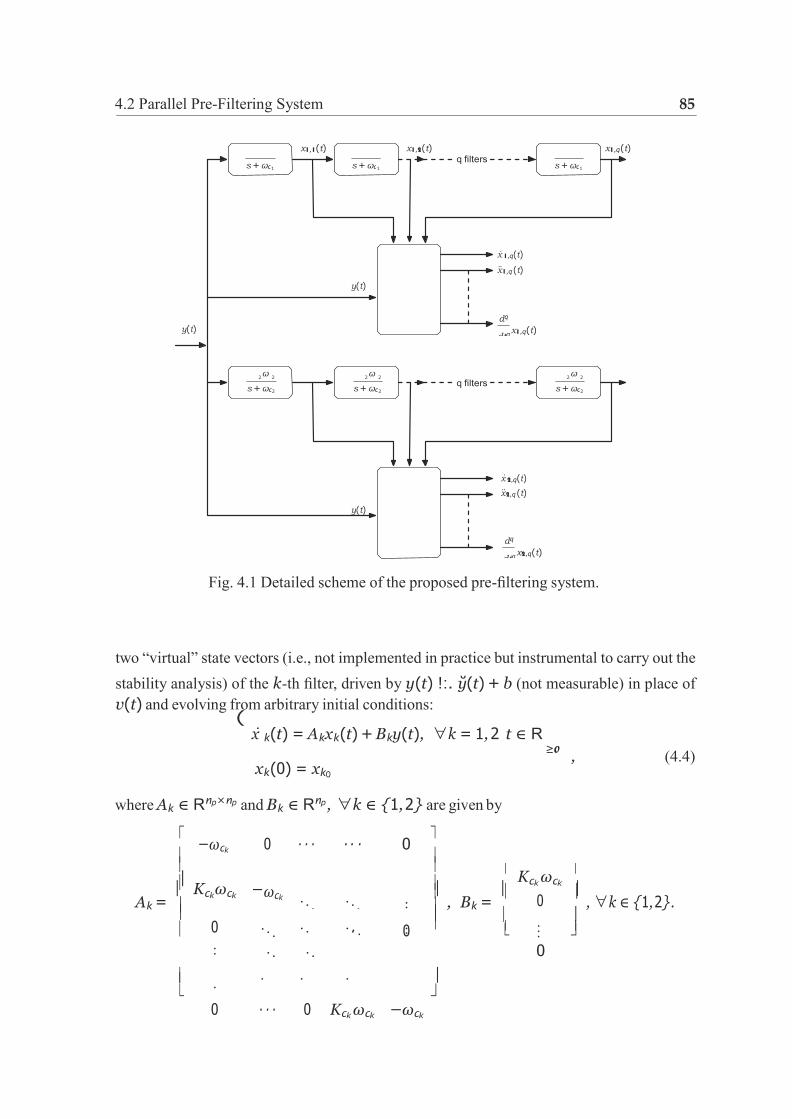
0
⎢
⎢ ⎢
4.2 Parallel Pre-Filtering System 85
Fig. 4.1 Detailed scheme of the proposed pre-filtering system.
two “virtual” state vectors (i.e., not implemented in practice but instrumental to carry out the
stability analysis) of the k-th filter, driven by y(t) !:. y(t) + b (not measurable) in place of
v(t) and evolving from arbitrary initial conditions: (
x k (t) = Akxk (t) + Bky(t), ∀k = 1, 2 t ∈ R
xk (0) = xk0
where Ak ∈ Rnp×np and Bk ∈ Rnp , ∀k ∈ 1, 2 are given by
≥0 , (4.4)
⎡ ⎤ −ωck 0 · · · · · · 0
⎢ ⎢ ⎢ ⎢ ⎢ ⎢
Kck ωck ⎢
Kck ωck ωck ⎢ ⎢
0 ⎢
Ak = ⎢ −
⎢
, Bk = ⎢
⎢
, ∀k ∈ 1, 2. ⎢ ⎢ ⎢
..
. . .
. . . .
⎢ ⎢ ⎢ . . 0 ⎢
⎢ ... ⎢
⎣ ⎦ 0
⎢ .
. . . ⎢ ⎣ ⎦
0 · · · 0 Kck ωck −ωck
x1,1(t) x1,2(t) x1,q (t)
s + ωc q filters
1 s + ωc 1 s + ωc 1
x 1,q (t)
x1,q (t)
y(t)
y(t) dq
dtq x1,q (t)
2 ω
2 2 ω
2
s + ωc 2 s + ωc q filters
2 ω
2
2 s + ωc 2
x 2,q (t)
x2,q (t)
y(t)
dq
dtq x2,q (t)
⎡ ⎤
. . . . . .
...
. . . . . .
...

86 STATE-VARIABLE FILTERING-BASED APPROACH
dti
ck
∞
The parameters ωc1 , ωc2 ∈ R>0, with ωc1 = ωc2 represent the poles of the low-pass filters,
while Kc1 , Kc2 ∈ (0, 1] play the role of damping gains. For the sake of further analysis, let
us introduce the combined virtual state vector x(t) = [x1(t) x2(t)]⊤
, which is governed by
the following differential equation, taking on the same form as in the nominal case (2.6):
x (t) = Apx(t) + Bpy(t), t ∈ R≥0 , (4.5)
with x(0) = [x⊤ , x⊤ ]⊤ and 10 20
Ap =
A1 0
0 A2
l
, Bp =
B1
l .
B2
Following the same procedure as in Sec 2.2.1, it is readily seen that in the time-domain the
derivatives di
x
k,np (t), 1 ≤ i ≤ np are available and tend asymptotically to the sinusoidal
regime as t → ∞. Let us consider the stationary sinusoidal conditions
di
dti xk,np (t) ≈ ak,i sin(ϕk,i(t)), ∀t >> 0, k ∈ 1, 2 , (4.6)
where ak,i = a ωi|Hk,n ( )|, ϕk,i(t) = ϕ(t) + ∠Hk,n ( ) +
π
i , (4.7)
with
p p 2
ωnp np
ck Kck
Hk,np (s) = (s + ω
)np .
Clearly, the derivative signals (4.6) are directly computable from the filters’ states (see (2.9))
and can be used as auxiliary signals to retrieve the frequency, the amplitude, and the phase of
the input sinusoid. It is clear that a high order perturbation can be dealt with by a sufficient
large np following the same procedure (see Section 2.2 for more details).
Theorem 4.2.1 (ISS of the parallel pre-filtering system) Given the sinusoidal signal y(t)
and the perturbed measurement v(t) (2.1), the error dynamics of the parallel pre-filtering
system (4.5) is ISS w.r.t. any additive disturbance signal d(t) ∈ L1 . D
Proof: The proof is trivial due to the fact that Ap < 0. It is thus omitted here (the reader is
referred to the single-filter case dealt with in Sec 2.2.2). •
Although the selection of np is not unique, the use of higher-order filters is not advisable
unless needed (e.g., in the presence of higher order perturbation, see Chapter 2) because of
the drawbacks of the higher order filtering (stated on page 27 in Sec. 2.2). To this end, in
the rest of this chapter, we first characterize the stability properties of a generalized parallel

4.3 Generic Order np + np Pre-Filtering-Based Frequency Estimator 87
pre-filtering-based estimation scheme, where each filter has order equal to np; the order can
be minimized to a 3 + 3 configuration characterized by the same unified convergence analysis.
Then, in Section 4.4, we further reduce the order yielding to a simplified 2 + 2 scheme the
stability analysis of which has to be carried out in a different way. Practically, the choice
of pre-filter’s configuration is determined by the designer depending on the performance
requested to the estimator. Indeed, in Section 4.7, we show that, at the cost of increasing
the order of the pre-filter, the 3 + 3 algorithm can provide an enhanced noise immunity in
contrast with the 2 + 2 technique.
4.3 Generic Order np + np Pre-Filtering-Based Frequency
Estimator
4.3.1 Underlying Idea
Without loss of generality, let us start from considering a parallel pre-filtering stage
having two pre-filters each of order np, where np ≥ 3. In correspondence to the available
auxiliary vectors
z1(t) =
dnp−2
dtnp−2 x1,np (t)
dnp−2 ⊤
dtnp−2 x2,np (t) ,
z2(t) =
dnp
dtnp x1,np (t)
dnp ⊤
dtnp x2,np (t) ,
(4.8)
formed by the derivatives of the internal pre-filter’s states, we introduce the counterparts in
the noise-free conditions:
z1(t) =
dnp−2
dtnp−2 x1,np (t)
dnp−2 ⊤
dtnp−2 x2,np (t)
, z2(t) =
dnp
dtnp x1,np (t)
dnp ⊤
dtnp x2,np (t) ,
which have the sinusoidal regime z1(t), z2(t). For simplicity, let us create the combined
vectors z(t) = [z1(t) z2(t)]⊤
, z(t) = [z1(t) z2(t)]⊤
, and the error vector in the presence of
d(t): z(t) = z(t) − z(t). The vector of auxiliary signals z(t) can be expressed directly in
terms of the available input y(t) and the np-th order filter’s states, x1(t) and x2(t):
I
z(t) = Φnp v(t) x1(t)⊤ x2(t)⊤
1⊤
, (4.9)

88 STATE-VARIABLE FILTERING-BASED APPROACH
2
1 0
with
0 CAnp−2
0 0 CA
np−2 Φnp = np−1 np
. CA1 B1 CA1 0 CA
np−1 np
2 B2 0 CA2
Accordingly, the “virtual” combined auxiliary derivatives z(t) = lz1(t)⊤ z2(t)⊤
l⊤ can be
expressed as I
z(t) = Φnp y(t) x1(t)⊤ x2(t)⊤
1⊤
. (4.10)
Moreover, the stationary sinusoids z1(t), z2(t) defined in (4.10) satisfy the equality
Ωz1(t) + z2(t) = 0.
We propose to obtain the unknown frequency of the measured signal by enforcing the above
constraint on the estimated one. To this end, the following gradient-based adaptation law
represents the core of the methodology, which exploits the available pre-filtered signals
z1(t), z2(t) in place of the unavailable pure sinusoids z1(t) and z2(t):
˙
Ω(t) = −µz1(t)⊤
(Ω (t)z1(t) + z2(t)
\
. (4.11)
Besides the frequency-adaptation mechanism just described, the pre-filter-based AFP scheme
also involves an amplitude and phase estimation method that will be described later on in
Section 4.5.
4.3.2 Stability Analysis of the Frequency Estimator
Assume the unknown sinusoidal regime x(t) induced by the initial filter’s state x0 gives
rise to a “virtual” signal vector z(t) that matches the stationary sinusoidal behavior since the
very beginning, when driven by the unperturbed sinusoid y(t), that is:
I
x(t) : Φnp y(t) x(t)⊤
1⊤
= z(t) = I z1(t)⊤ z2(t)⊤
1⊤
, ∀t ∈ R≥0. (4.12)
The ISS of the error dynamics x(t) claimed in Theorem 4.2.1 immediately implies that
z(t) /'. z(t) − z(t) is ISS due to the identities (4.9) and (4.10). The error trajectory will enter
in finite-time in a closed ball of radius γz (d) + δ centered at the origin, where
γz (r) = Φnp (γx(r) + r), ∀r ∈ R≥0, δ = Φnp υ (4.13)

4.3 Generic Order np + np Pre-Filtering-Based Frequency Estimator 89
npπ
p
and where Φnp ≥ ∥Φnp ∥.
Introducing the frequency estimation error Ω (t) /'. Ω (t) − Ω, and applying the identity
z2(t) = −Ωz1(t), the dynamics of the frequency estimation error Ω (t) evolves according to
Ω˙ (t) = −µ(z1(t) + z1(t))⊤
(Ω (t)(z1(t) + z1(t)) − Ωz1(t) + z2(t)
\
= −µΩ z1(t)⊤z1(t) + µΩ f1(t, z) + µf2(t, z) , (4.14)
where f1(t, z) = −2z1(t)⊤z1(t) − z1(t)⊤z1(t)
f2(t, z) = Ω(f1(t, z) + z1(t)⊤z1(t)) − z1(t)⊤z2(t).
Note that the functions f1(t, z) and f2(t, z) verify f1(t, 0) = 0, f2(t, 0) = 0 for all t ∈ R≥0.
Moreover, owing to the boundedness of z(t), there exist two K∞-functions γf,1(·) and γf,2(·)
such that
|f1(t, z)| ≤ γf,1(|z|) , |f2(t, z)| ≤ γf,2(|z|) . (4.15)
The following assumption is needed to prove the convergence of the estimation error.
Assumption 4 The signal z1(t) is persistently exciting in the sense that there exist a constant
o > 0 such that
z1(t)⊤z1(t) ≥ ε, ∀t > 0. (4.16)
In the following derivations, we show that Assumption 4 is verified under a suitable choice
of ωc1 and ωc2 in the nominal (noise-free) condition. Let us expand z1(t)⊤z1(t) as follows:
dnp−2x1,n
dnp−2x2,n
z1(t)⊤z1(t) = dtn
2 p−2
(t) + dtnp−2 (t)
π
= ak,n
k=1
2 sin2 (ϕ(t) + ϕ k,np
+
\
2 (np − 2) ,
where ak,np−2 = aω
algebra, we get
np−2 |Hk,np ( )| and ϕk,np denotes the phase of Hk,np ( ). After some
ϕ1,np = np arctan ω
− ωc
, ϕ2,np = np arctan
ω
− ωc
Thanks to the fact that |ϕ1,np − ϕ2,np | <
t > 0 if
2 , ∀ω > 0, z1(t)⊤ z1(t) is strictly positive for
|ϕ1,np − ϕ2,np | = jπ, j ∈ [0, 1, 2, ....⌊np/2⌋), ∀ω ∈ R>0 (4.17)
1 2
2 p
2
p−
.

90 STATE-VARIABLE FILTERING-BASED APPROACH
±
with ⌊·⌋ being the floor operator.
In view of (4.17), it is readily seen that |ϕ1,np − ϕ2,np | = 0, i.e., ϕ1,np = ϕ2,np , ∀ω > 0
as long as ωc1 and ωc2 are distinct. Next, we show a choice of the pre-filters’ parameters such
that ω2 2 2
c1 + ωc2
− (2 + 4α )ωc1 ωc2 < 0 , (4.18)
where α = tan(π/np), implies that the condition |ϕ1,np −ϕ2,np | = jπ, j ∈ [1, 2, ....⌊np/2⌋), ∀ω >
0 is satisfied. Let us suppose that there exists ω ∈ R>0, such that |ϕ1,np − ϕ2,np | = jπ. Such
hypothesis holds if and only if
arctan
ω
ωc1 — arctan
ω jπ
= . ωc2 np
Taking tan(·) on both hand side of the above equation, and owing to the property of trigono-
metric functions, we get
ω
ωc1
ω
ωc2
/ 1 + ω2
ωc1 ωc2 = ± tan(jπ/np)
which can be rearranged as follows:
tan(jπ/np)ω2 ± (ωc — ωc )ω + tan(jπ/np)ωc ωc = 0 . (4.19) 1 2 1 2
Note that equation (4.19) does not admit any real root in the variable ω as long as
ω2 2 2
c1 + ωc2
− (2 + 4 tan(jπ/np) )ωc1 ωc2 < 0,
which is always true if (4.18) holds since 0 < tan(π/np) ≤ tan(jπ/np) < tan(π/2).
Therefore, by contradiction, the condition
|ϕ1,np − φ2,np | = jπ, j ∈ [0, 1, 2, ....⌊np/2⌋), ∀ω ∈ R>0
can be ensured by proper selection of ωc1 , ωc2 . Finally, due to the phase separation property,
there always exist a positive constant ε, such that excitation condition (4.16) is verified for
all t > 0.
Theorem 4.3.1 (ISS of the adaptive frequency identifier) Under Assumption 4, given the
sinusoidal signal y(t) and the perturbed measurement model (4.1), the frequency estimation
system made up of the two filters (4.4) of order n (n ≥ 3) and by the adaptation law (4.9)
−

4.3 Generic Order np + np Pre-Filtering-Based Frequency Estimator 91
∞
∞ z f,1
2
Ω (t) ≤ −µ(ε − γ
2
⊤
and (4.11) is ISS w.r.t. any additive disturbance signal d(t) ∈ L1 such that
∥d∥ < d < γ−1 ( γ
−1(ε)) , (4.20)
where γz and γf,1 are given by (4.13) and (4.15), respectively. D
Proof: According to (4.13), for any positive δ ∈ R>0 there exists a finite time-instant Tδ such
that |z(t)| ≤ γz (d) + δ, ∀t ≥ Tδ , which implies
γf,1(|z(t)|) ≤ γf,1(γz (d) + δ), ∀t ≥ Tδ. (4.21)
If the bound (4.20) on the disturbances holds, then, for some δ ∈ R>0, the following
inequality is satisfied
ε − γf,1(γz (d) + δ) > 0. (4.22)
Thus, in view of (4.14), (4.15) and Assumption 4, the following bound on the derivative of
candidate Lyapunov function V = 1 Ω 2 can be established for any t > Tδ :
∂ V ˙
∂Ω
f,1 (γz (d) + δ)\|Ω (t)|2 + µγ
f,2 (|z(t)|)|Ω (t)|
(4.23)
≤ −∆µ |Ω (t)|2 + µγf,2(|z(t)|)|Ω (t)|, t ≥ Tδ ,
where ∆µ /'. µ lε − γf,1(γz (d) + δ)
l is a positive constant. Thus, Ω (t) is ISS w.r.t. z(t) and
in turn, ISS w.r.t. d. •
4.3.3 Pre-Filter of Order 3 + 3
In this paragraph, we specialize the previous scheme to the case np = 3. Considering
np = 3 in (4.8), the auxiliary vectors are:
z1(t) = Ix
1,3(t) x 2,3(t)
1 ,
z2(t) =
d3
dt3
x1,3(t) d3
dt3
⊤
x2,3(t) ,
formed by the derivatives of the internal pre-filter’s states of order 3. For simplicity, let
us consider the combined vector of auxiliary signals z(t) = [z1(t) z2(t)]⊤
which can be
expressed directly in terms of the available measurement v(t) and the pre-filter’s states
xk (t) ∈ R3, k = 1, 2:
z(t) = Φ3
I v(t) x1(t)⊤ x (t)⊤
1⊤
, (4.24)

92 STATE-VARIABLE FILTERING-BASED APPROACH
Φ =
2 −−−→ 2 1
1 −−−→ 1 1,0 1,0 2,0 2,0
2 2
with
3
.
CA2B1 CA3 0 1 1
CA2B2 0 CA3
2 2
Finally, the frequency is estimated by the recursive algorithm (4.11) on the basis of the
updated z1(t) and z2(t). The stability analysis of the 3 + 3 frequency estimator is a special
case of the one given in Section 4.3.2 and is therefore omitted.
4.4 Order 2 + 2 Pre-Filtering-Based Frequency Estimator
4.4.1 Underlying Idea
In this section, we aim to further reduce the dynamic order of the estimator, by decreasing
the order of the two pre-filters to np = 2. Let us choose Kc1 = Kc2 = Kc and then introduce the auxiliary signals z1(t) = x1,2(t) − x2,2(t) and z2(t) = d x (t) − d x (t). It is easy
dt2 1,2 dt2 2,2
to show that both z1 and z2 tend asymptotically to a sinusoidal regime given by:
z (t) t→∞
z (t) = a sin(ϕ (t)) − a sin(ϕ (t)) ,
z (t) t→∞
z (t) = −Ωz (t) ,
with Ω = ω2 is the true (unknown) squared-frequency, and where
(4.25)
ak,0 = a |Hk,2( )|, ϕk,0(t) = ϕ(t) + ∠Hk,2( ). (4.26)
with
ω2 K2
Hk,2(s) = ck c 2
(s + ωck )
In view of (4.25), z1(t) turns out to be a pure single sinusoidal signal having frequency ω
and amplitude
az1 = I
y2 + y2 , (4.27) p q
in which
yp = a1,0 cos ∠H1,2( ) − a2,0 cos ∠H2,2( ),
yq = a1,0 sin ∠H1,2( ω) − a2,0 sin ∠H2,2( ω) .
Similar to the order np + np algorithm, the following gradient-based adaptation law that
exploits the available pre-filtered signals z1(t), z2(t) in place of the unavailable pure sinusoids
.
0 CA1 0
0 0 CA2
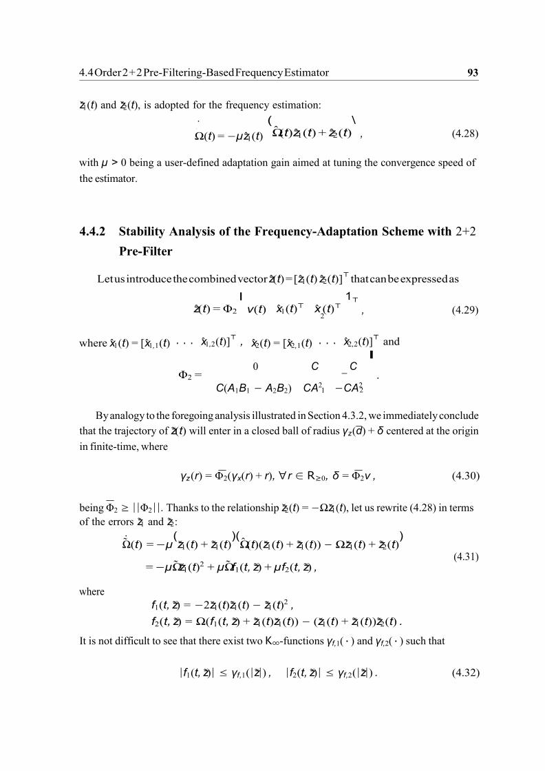
4.4 Order 2 + 2 Pre-Filtering-Based Frequency Estimator 93
2
1 2
−
z1(t) and z2(t), is adopted for the frequency estimation:
˙ Ω(t) = −µz1(t)
(Ω (t)z1(t) + z2(t)
\ , (4.28)
with µ > 0 being a user-defined adaptation gain aimed at tuning the convergence speed of
the estimator.
4.4.2 Stability Analysis of the Frequency-Adaptation Scheme with 2+2
Pre-Filter
Let us introduce the combined vector z(t) = [z1(t) z2(t)]⊤
that can be expressed as
z(t) = Φ2
I v(t) x1(t)⊤ x (t)⊤
1⊤
, (4.29)
where x1(t) = [x1,1(t) · · · x1,2(t)]⊤
, x2(t) = [x2,1(t) · · · x2,2(t)]⊤
and
Φ2 =
0 C C
l .
C(A1B1 − A2B2) CA2 −CA2
By analogy to the foregoing analysis illustrated in Section 4.3.2, we immediately conclude
that the trajectory of z(t) will enter in a closed ball of radius γz (d) + δ centered at the origin
in finite-time, where
γz (r) = Φ2(γx(r) + r), ∀r ∈ R≥0, δ = Φ2ν , (4.30)
being Φ2 ≥ ||Φ2||. Thanks to the relationship z2(t) = −Ωz1(t), let us rewrite (4.28) in terms
of the errors z1 and z2:
Ω˙
(t) = −µ(z1(t) + z1(t)
)(Ω (t)(z1(t) + z1(t)) − Ωz1(t) + z2(t)
)
= −µΩ z1(t)2 + µΩ f1(t, z) + µf2(t, z) , (4.31)
where
f1(t, z) = −2z1(t)z1(t) − z1(t)2 ,
f2(t, z) = Ω(f1(t, z) + z1(t)z1(t)) − (z1(t) + z1(t))z2(t) .
It is not difficult to see that there exist two K∞-functions γf,1(·) and γf,2(·) such that
|f1(t, z)| ≤ γf,1(|z|) , |f2(t, z)| ≤ γf,2(|z|) . (4.32)

94 STATE-VARIABLE FILTERING-BASED APPROACH
z1
z z1
z1
z1 z1
1
z1
The following result characterizes the stability properties of the frequency estimator.
Theorem 4.4.1 (ISS of the adaptive frequency identifier) Given the sinusoidal signal v(t)
and the perturbed measurement model (2.1), let the bound on the measurement disturbance
d verify the inequality:
1 −1
ωκa2
ln ((1 − κ∆)/κ)
||d||∞ < d < γ− γf,1
µπκa2 − 2ω ln (1/κ) , (4.33)
where az1 is given by (4.27), κ : κ ∈ (0, 1) is chosen arbitrarily, κ∆ ∈ R>0 is such that
1 − κ∆ > κ, and µ is chosen large enough to verify the following two inequalities:
ω ln (1/κ)/(µκa2 ) < π (4.34)
and cos2
ω ln (1/κ)
— κ ≥ ωκ ln ((1 − κ∆)/κ)
. (4.35) 2µκa2 µπκa2 − 2ω ln (1/κ)
Then, the frequency estimation system given by the two filters (4.5) with n = 2 and by (4.28)
and (4.29) is ISS w.r.t. d(t). D
Proof: Consider the following candidate Lyapunov function V (Ω ) = 1
Ω 2. In view of (4.31) 2
and (4.32), the time-derivative of V (t) along the system’s trajectory satisfies:
∂V ˆ ˜ ˜ 2 ˜ 2 ˜
∂Ω Ω(t) = Ω(t)Ω(t) ≤ −µ(z1(t) − γf,1(|z(t)|)) Ω(t) + µγf,2(|z(t)|)|Ω(t)| , (4.36)
in which the stationary sinusoidal signal z1(t) appears explicitly. Now, under the assumption
of d given by (4.33) and the inequalities (4.34) and (4.35), then the period of the squared
sinusoid z2(t) can be partitioned in three intervals: P2, in which it holds that
(z1(t)2 − γf,1(γz (d) + δ)
) ≥ κa2
and P1, P3, in which this inequality is not guaranteed. In the following, we denote by t0,
t1 and t2 the transition time-instants between the aforementioned modes of behavior, as
described in Fig.4.2. Without loss of generality, the duration of P2 is denoted by Te that is subject to Te ≤ π , while the duration of P1 and P3 are identical denoted by Td = π − Te
ω 2ω 2
We prove that there exist a suitably specified constant, such that if the interval P2 lasts for
more than Te, then the discrete-time Lyapunov function obtained by sampling the continuous-
time Lyapunov function at the end of the three phases is a discrete-ISS Lyapunov function.
.
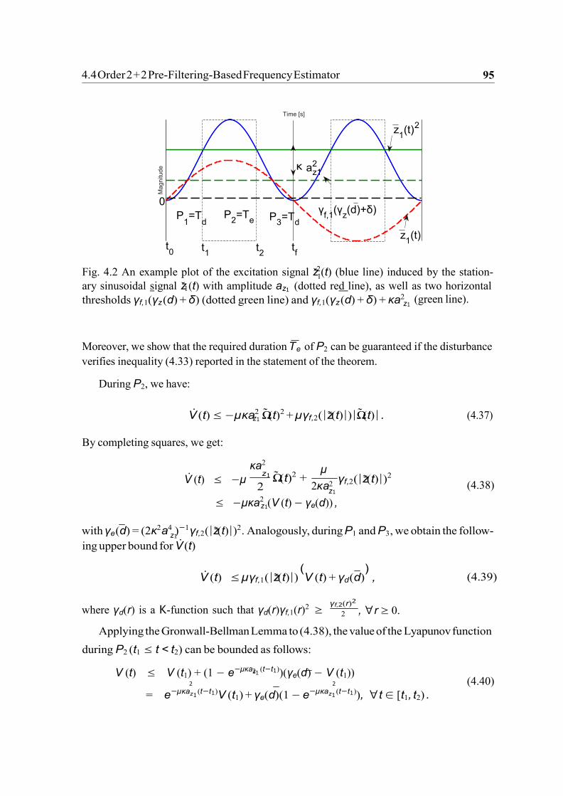
4.4 Order 2 + 2 Pre-Filtering-Based Frequency Estimator 95
1
z1
z1
z1
z1
z1
2
Ma
gn
itu
de
Time [s]
z1(t)
a2 z1
0
P1=T
d P
2=T
e
t0 t
1 t2
P
3=T
d
tf
γf,1
(γz(d)+δ)
z1(t)
Fig. 4.2 An example plot of the excitation signal z2(t) (blue line) induced by the station-
ary sinusoidal signal z1(t) with amplitude az1 (dotted red line), as well as two horizontal
thresholds γf,1(γz (d) + δ) (dotted green line) and γf,1(γz (d) + δ) + κa2 (green line).
Moreover, we show that the required duration Te of P2 can be guaranteed if the disturbance
verifies inequality (4.33) reported in the statement of the theorem.
During P2, we have:
V (t) ≤ −µκa2 Ω (t)2 + µγf,2(|z(t)|)|Ω (t)| . (4.37)
By completing squares, we get:
V (t) ≤ −µ
κa2
z1 Ω (t)2 + 2
µ
2κ a2 γf,2(|z(t)|)2
(4.38)
≤ −µκa2 (V (t) − γe(d)) ,
with γe(d) = (2κ2a4 )−1γf,2(|z(t)|)2. Analogously, during P1 and P3, we obtain the follow-
ing upper bound for V (t)
V (t) ≤ µγf,1(|z(t)|) (V (t) + γd(d)
) , (4.39)
where γd(r) is a K-function such that γd(r)γf,1(r)2 ≥
γf,2(r)2
2 , ∀r ≥ 0.
Applying the Gronwall-Bellman Lemma to (4.38), the value of the Lyapunov function
during P2 (t1 ≤ t < t2) can be bounded as follows:
V (t) ≤ V (t1) + (1 − e−µκaz1 (t−t1))(γe(d) − V (t1))
2 2 (4.40)
= e−µκaz1 (t−t1)V (t1) + γe(d)(1 − e−µκaz1
(t−t1)), ∀t ∈ [t1, t2) .
κ
2

96 STATE-VARIABLE FILTERING-BASED APPROACH
ω
1
2
z1
z1
z1
2
z1
Taking the same steps as above, we obtain a further bound of V (t) during the “dis-excited”
intervals P1 and P3:
V (t) ≤ V (tp)eµγf,1(|z(t)|)(t−tp) + (eµγf,1(|z(t)|)(t−tp) − 1)γd(d), π
∀t ∈ [t0, t1), if p = 0 or ∀t ∈ [t2, t0 + ω
), if p = 2 . (4.41)
Due to the poor excitation during P1 and P3, at the end of these intervals we can establish a
(possibly) conservative bound
V (te) ≤ eµγf,1(|z(t)|)Td (V (tp) + γd(d)
) , te = t1, if p = 0 (i.e., in P1)
or t = t + π
, if p = 2 (i.e., in P ) . (4.42) e 0
ω 3
Then, in view of (4.40), assuming that the mode P2 occurs for a time Te (we do not pose a
lower-bound on Te at this point, possibly Te = 0 ), we get the inequality:
2 2
V (t2) ≤ e−µκaz1 Te
leµγf,1(|z(t)|)Td
(V (t0) + γd(d)
)l + γe(d)(1 − e−µκaz1
Te ) . (4.43)
Finally, denoting by Vk /'. V (t0 + k π
) the value of the Lyapunov function at the end of each
k-th P3 interval, and considering that t0 is arbitrary within the set t0 ∈ t : z2(t) = 0, from
inequalities (4.42) and (4.43), we can easily get the following expression:
2 2
Vk+1 ≤ e2µγf,1(|z(t)|)Td−µκaz1 Te Vk + γe(d)(1 − e−µκaz1
Te )eµγf,1(|z(t)|)Td
+ (e2µγf,1(|z(t)|)Td−µκaz1 Te + eµγf,1(|z(t)|)Td )γd(d) . (4.44)
We now show that a minimum time-duration of phase P2, denoted by Te, is ensured as long
as the bound (4.33) is verified. Indeed (4.33) implies that
γf,1(γz (d) + δ) < ωκa2
ln ((1 − κ∆)/κ)
µπκa2 − 2ω ln (1/κ) (4.45)
= ln ((1 − κ∆)/κ)
.
2µ(π/2ω − ln (1/κ)/µκa2 )
Then, thanks to (4.35), there exists a positive constant Td that bounds the length of the
dis-excitation interval (Td ≤ Td) :
( π 2 2 ω ln (1/κ)
T d /'. min t ≤ ω
: z1(t0 + t) ≥ az1 cos 2µκa2
.

4.4 Order 2 + 2 Pre-Filtering-Based Frequency Estimator 97
z1
a2 z1
z1
z1
z1
z1
Owing to the fact that z1(t0 + T d)2 = a2 sin2(ω(t0 + T d)), then Td can be computed as the
minimum positive solution of the equation:
ω ln (1/κ)
z1 sin
2 (ωT d
) = a2 cos 2 . 2µκa2
From (4.34), it holds that
Hence,
π
T d = 2ω
−
π
Te ≥ ω
− 2T d ≥
ln (1/κ)
2µκa2
ln (1/κ)
µκa2
.
= T e.
Combining T d and (4.45), we also get
e2µγf,1(|z(t)|)Td < e2µγf,1(|z(t)|)T d < (1 − κ∆)
. κ
Next, we prove that the Lyapunov function with discrete dynamics induced by sampling
the frequency estimator in correspondence of the transitions is ISS with respect to the
measurement disturbance d(t). Since
t2 − t1 = Te ≥ ln (1/κ)
µκa2 ,
picking ϵ ∈ R>0 such that 1 − κ∆ < ϵ < 1, then we can guarantee the following bound on
the discrete (sampled) Lyapunov function sequence:
1 1
Vk+1 ≤ ϵVk + γe(d)(1 − κ) √κ
+ (1 + √κ
)γd(d) .
In compact form:
Vk+1 − Vk ≤ −(1 − ϵ)Vk + γv (d) ,
where the function γv (·) is a K-function defined as
1 1
γv (r) = γe(r)(1 − κ) √κ
+ (1 + √κ
)γd(r), ∀r ∈ R≥0 .
Hence, we are able to conclude that Vk is a discrete ISS Lyapunov function for the sampled
sequence.
Finally, we show the ISS for the continuous-time system by using the continuity ofV (t)
and the boundedness of its time-derivative in the inter-sampling. Thanks to the periodicity

98 STATE-VARIABLE FILTERING-BASED APPROACH
√
−−−→
(
of the excitation signal z1(t)2, let us denote by t0(k), t1(k) and t2(k) the transition time-
instants of the k-th period of z1(t)2, and k(t) the index of the current period: k(t) = k : t ∈ lt0(k), t0(k + 1)
). Between two samples, the Lyapunov function can be bounded (possibly
in a conservative way) by,
1 ) l
V (t) ≤ √κ
lV (t0) + γd(d)
l + l
κ V (t0) + γd(d)
1
+ γe(d)
1
+ V (t0) + √κγe(d) + (1 + √
κ )γd(d)
1 + √
κ + κ 1 2
= √κ
Vk(t) + (1 + √κ
)γe(d) + (2 + √κ
)γd(d) . (4.46)
Since k(t) t→∞
∞, an infinite number of excited phases with length Te occurs asymptoti-
cally; the estimation error in the inter-sampling times converges to a compact region whose
radius depends on the bound on the disturbance (assumed to exist), hence concluding the
proof. •
4.5 Amplitude and Phase Estimation
Finally, we propose a unified algorithm for estimating the amplitude and the phase that
applies to all the np + np (np ≥ 2) methods presented in this chapter. Following the same
procedure carried out in Section 2.3, the amplitude and phase (ak,q, ϕk,q ) of the q-th derivative
of the np-th state variable of the k-th pre-filter (see (4.6) and (4.7)) can be estimated as follows
by using ω(t) obtained by either methods illustrated in this chapter:
I
dq−1 2
dq 2
ak,q (t) = I
Ω (t) dtq−1 xk,np (t) + dtq
xk,np (t) , (4.47a)
dq
dq−1
ϕk,q (t) = ∠ dtq
xk,np (t) + ω(t) dtq−1
xk,np (t) , ∀q ≤ np , (4.47b)
and
a(t) =
ak,q (t)
II ω2
+ ω(t)2/(Kc
ωc )
1np
, (4.48a) ω(t)q ck k k
π
ϕ(t) = ϕk,q (t) + np arctan(ω(t)/ωck ) − 2
q . (4.48b)

2
Φ =
2 2
2
4.6 Digital implementation of the proposed method 99
The “ill” defined non-adaptive formulas (4.47a) and (4.48a) (they are not defined when
ω(t) = 0) are amended by the following adaptive mechanisms:
I
a k,q (t) = −µa ak,q (t) −
I
Ω(t)
dq−1 2
xk,n (t)
dq
+ xk,n (t)
2
(4.49)
ˆ
dtq−1 p
dtq p
and
a (t) = −µaω(t)q ω(t)q a(t) − ak,q (t)
I
+ ω(t)2/(Kc
ωck
1np
)
(4.50)
with initial condition ak,q (0) = 0, a(0) = 0 and tunable parameters µa ∈ R>0 that determine
the rate of convergence. The above adaption laws makes it easy to enforce, simply by a
clipping (e.g., (3.11)), the positivity constraints a ≥ 0.
4.6 Digital implementation of the proposed method
In this section, we briefly illustrate the digital implementation of the introduced algo-
rithms. Consider a measured signal v(k), k = 1, 2, · · · sampled by Ts, we firstly make a
choice of the tunable parameters ωc1 , ωc2 , Kc1 , Kc2 , µ. It is worth noting that both methods
rely on the filtered signals obtained by the parallel pre-filtering system (4.5), which in the
discrete-time domain is represented by
x(k) = x(k − 1) + Ts (Apx(k − 1) + Bpv(k)) , (4.51)
where x(t) = [x1(t) x2(t)]⊤
, x1(t) = [x1,1(t) · · · x1,2(t)]⊤
, x2(t) = [x2,1(t) · · · x2,2(t)]⊤
.
Thanks to (4.51), the auxiliary signal z(k) for the method 1 (see Section 4.3.3) is obtained by
z(k) = Φ3
I v(k) x1(k)⊤ x (k)⊤
1⊤
,
with 0 CA1 0
0 0 CA2
3 CA2B1 CA3 0
1
CA2B2
1
0 CA3
On the other side, for method 2 (see Section 4.4), we get
z(k) = Φ2
I v(k) x1(k)⊤ x (k)⊤
1⊤
,
ω 2 I
ck k
.

100 STATE-VARIABLE FILTERING-BASED APPROACH
1 2
−
with
Φ2 =
0 C C
l .
C(A1B1 − A2B2) CA2 −CA2
The frequency adaptation laws for both methods have the same representation, which in the
discrete-time domain writes:
Ω (k) = Ω (k − 1) − Tsµz1(k) (Ω (k − 1)z1(k) + z2(k)
\ ,
I
ω(k) = max0, Ω (k)
where z1(k), z2(k) for method 1 are vectors, however for method 2 they are scalars.
Finally, by using z(t) and ω(k), it is straightforward to estimate the amplitude and the
phase by the discretized equations of (4.49), (4.50), (4.47b) and (4.48b).
4.7 Simulation and Experimental Results 4.7.1 Simulation Results
In this subsection, the behaviour of the proposed methods are evaluated and compared
with three recently proposed AFP techniques [58], [28] and [90]. All the algorithms are
discretized by Forward-Euler discretization method with fixed sampling period 1 × 10⁻³s.
The algorithms considered in the comparative analysis have been tuned to have a similar
response time when fed by a unitary-amplitude sinusoid of frequency 1/(2π), when initialized
with zero initial conditions (indeed, the initial transient of the frequency-estimates shown in
Fig.4.3 put in evidence that the considered methods share the same rise-time). The evaluations
are conducted in the case of a biased sinusoidal signal, undergoing both frequency and offset
steps-wise variations.
Let us consider a sinusoidal measurement corrupted by a bounded disturbance:
v(t) = b(t) + 3 sin(ω(t) t + π/4) + d(t), (4.52)
with
ω(t) =
4, 0 ≤ t < 10 8, 10 ≤ t < 35
, b(t) =
( 1, 0 ≤
t < 20
. 2 35 ≤ t < 50
3 20 ≤ t < 50
d(t) is a bounded disturbance with uniform distribution in the interval [-0.5, 0.5]. All the
methods are initialized with the same initial condition ω(0) = 1. Method [58] is tuned
with: µ0 = 1.5, µ1 = 3, µ2 = 3, µ3 = 0.8, while method [28] is tuned with: Ks = 1, λ =

4.7 Simulation and Experimental Results 101
0
1, ωs = 4, Q0 = (1/λ)I. For method [90], we set γ0 = λ2 = 8, γ1 = 6, k = 0.18. Finally,
the tuning parameters of the proposed methods are selected by: ωc1 = 6, ωc2 = 3, Kc1 =
0.6, Kc2 = 0.8 , µ = 1 and ωc1 = 9, ωc2 = 2, Kc1 = Kc2 = 0.6, µ = 4 respectively
(heuristic tuning guidelines of the pre-filtering parameters ωck , Kck and the adaptive gain µ
can be referred to the Figure 2.4 and 2.5). The frequency-estimation trends obtained by the
simulations are depicted in Fig.4.3.
Estimated Frequencies from a biased and noisy input signal 10
AFP method [91]
AFP method [29]
8 PLL method [59]
Method 2 (’2+2’)
Method 1 (’3+3’) 6
4
2
0
0 5 10 15 20 25 30 35 40 45 50
Time [s]
Fig. 4.3 Time-behavior of the estimated frequency by using the proposed AFP methods (blue
and red line respectively) compared with the time behaviors of the estimated frequency by
the AFP methods [28] (black line), [58] (green line) and [90] (cyan line).
All the methods are capable to track the initial frequency satisfactorily, with similar
response time (the constraint for choosing parameters). The PLL method [58] exhibits a
good noise immunity in stationary conditions, but is quite slow to track frequency variations,
specially in the low-frequency range. The AFP method [28] is the more sensitive to the
bias change, however, it performs the best noise attenuation at the cost of slow reaction to a
significant frequency change. The proposed methods can handle considerable frequency vari-
ations with relatively fast response time and acceptable robustness against noise. Compared
to the single pre-filter-based method [90] (note that the switching dynamic consists in this
algorithm is switched off in order to consider the time-varying frequency), in this example
the presented methods equipped with parallel pre-filters show certain improvements in terms
of noise immunity without deteriorating the transient performance.
The amplitude estimates of each method are reported in Fig.4.4 ([90] is excluded, since
it only deals with frequency estimation). Among the three recursive algorithms, the PLL
method [58] is the simplest in terms of dynamic order, but it is prone to be affected by the
parametric perturbations. On the other hand, the proposed methods estimate the amplitude
in a relatively smoother manner, in particular, method 1 (see Section 4.3) provides the best
noise immunity in the stationary phases.
Fre
qu
en
cy [
rad
/s]

102 STATE-VARIABLE FILTERING-BASED APPROACH
Estimated Amplitudes from a biased and noisy input signal
5
Overshoot over18
4
3
2
1
0 AFP method [29]
PLL method [59]
−1 Method 2 (’2+2’)
Method 2 (’3+3’) −2
0 5 10 15 20 25 30 35 40 45 50
Time [s]
Fig. 4.4 Time-behavior of the estimated amplitude by using the proposed AFP methods (blue
and red line respectively) compared with the time behaviors of the estimated frequency by
the AFP methods [28] (black line) and [58] (green line).
Thanks to the availability of the phase estimation, the sinusoidal signal reconstructed
by the proposed method is depicted in Fig.4.5, in which the unbiased signal is recovered
successfully in a smooth manner even the input is affected by a bounded uncertainty.
8 Unbiased input
Biased input
Sinusoidal signal reconstruction
6 Estimated sinusoid
4
2
0
−2
−4
−6 0 5 10 15 20 25 30 35 40 45 50
Time [s]
Fig. 4.5 Estimated sinusoidal signal by the proposed AFP method 2 (blue line). To appreciate
the time-behavior of the estimated signal, the biased noisy input is depicted (red line), as
well as the same signal without the time-varying bias term (green line).
In order to complete the comparison of the proposed methods, in Fig.4.6, the time-
behaviors of the estimated frequency are shown in another case in which higher level of
noise affects the input. It can be observed that method 1 with an order 3 + 3 configuration
(see Section 4.3) offers slightly better steady state performance at the expense of increased
complexity.
Inp
ut and
estim
ate
d s
igna
ls
Am
plit
ud
e

4.7 Simulation and Experimental Results 103
Estimated Frequencies from a biased input signal with intensive noise: noise u.d.in [−5,5]
10
8
6
4
2
0
0 5 10 15 20 25 30 35 40 45 50
Time [s]
Fig. 4.6 Comparison of the behaviors of the proposed AFP method 1 (blue line) and 2 (red
line) in the presence of a bounded perturbation within the interval [−5, 5].
4.7.2 Experimental Results
In order to evaluate the robustness of the proposed algorithm in practice, we have
deployed the method 2 introduced in Section 4.4 on a dSpace system. In order to confirm
the simulation results on an experimental test-rig, the two prior methods [58] and [28] have
been implemented in the same system, with the task of estimating the frequency, the phase
and amplitude of an electrical voltage signal generated by a programmable power supply
able to reproduce the perturbations typically experienced in micro-grids. Note that all the
methodologies are discretized by Euler method with sampling rate set to 60kHz. Fig. 4.7
shows some periods of the noisy sinusoidal signal generated by the programmable power
supply. The large voltage ripples superimposed on the measured sinusoid correspond to the
perturbations that may arise from the switching actions of grid-connected power electronic
devices. On the other side, voltage-injected spikes are used to reproduce the large voltage
transients due to the sudden change of electric loads or to severe radio frequency interference
such as those caused by lightning.
In the first test, the frequency of the supply is varied according to the following pattern:
50-48-50-52-48Hz (which is likely to occur on a small-scale power system such as a micro-
grid). In particular, the frequency changes are composed of multiple steps in order to
imitate the inertia of electro-mechanical generators. The tuning gains of the methods [58]
and [28] are set to the following values: µ0 = 15, µ1 = µ2 = 300, µ3 = 0.07 and
Ks = 1, λ = 10, ωs = 2π50, Q0 = (1/λ)I , while the parameters of the proposed estimator
are: ωc1 = 320, ωc2 = 250, Kc1 = Kc2 = 0.6, µ1 = 50. The dSpace board computes the
frequency estimates in real-time and converts them to analog signals that are collected by an
Fre
qu
en
cy [
rad
/s]
Method 2 (’2+2’)
Method 2 (’3+3’)

104 STATE-VARIABLE FILTERING-BASED APPROACH
Sig
na
l
2.5
Practical sinusoidal input
2
1.5
1
0.5
0
-0.5
-1
-1.5
-2
-2.5
0 0.01 0.02 0.03 0.04 0.05 0.06 0.07 0.08 0.09 0.1
Time [s]
Fig. 4.7 A real-time 50 Hz sinusoidal voltage signal corrupted by ripples reproducing the
perturbation due to a typical switching device and 4 large spikes per cycle to reproduce RF
interference.
oscilloscope whose plot is given in Fig. 4.8. The estimates show that all the methods can be
adjusted to achieve a similar response time to the given frequency step-wise variations.
Estimated frequency from a practical input with spikes and step frequency changes
52.5
52
51.5
51
50.5
50
49.5
49
48.5
48
47.5
0 2 4 6 8 10 12 14 16 18 20
Time [s]
Fig. 4.8 Real-time frequency tracking of a sinusoidal signal with a step-wise changing
frequency (50-48-50-52-48 Hz): the time behaviors of the estimated frequency by the AFP
methods [28] (greed line), [58] (red line) and the proposed method 2 (blue lines).
For the sake of completeness, with the fixed parameter setting the robustness against bias
variations is tested by introducing a measurement offset with step-wise changes (0-0.5-0)
over the alternating current voltage signal given in Fig. 4.7 . According to the results shown
Fre
quen
cy [H
z]

4.8 Concluding Remarks 105
in Fig. 4.9, the proposed method shows an enhanced transient behavior with only minor loss
on the stationary accuracy compared with the other two approaches.
51.5 Estimated frequency from practical input with spiks and step bias changes
51
50.5
50
49.5
49
48.5
48
47.5
47
46.5 0 0.2 0.4 0.6 0.8 1 1.2 1.4 1.6
Time [s]
Fig. 4.9 Real-time frequency tracking of a sinusoidal signal with a step-wise changing offset:
the time behaviors of the estimated frequency by the AFP methods [28] (greed line), [58]
(red line) and the proposed method 2 (blue lines).
4.8 Concluding Remarks
This chapter deals with an AFP scheme based on the parallel pre-filtering paradigm
with the aim of reducing the dynamic order of the adaptive observer approach introduced in
Chapter 2. The parallel pre-filtering methodology consists in filtering a noisy-biased sinusoid
with a pair of two low-pass filters of a given order, whose inner states are used to estimate
the frequency, the phase and the amplitude of the original sinusoid. The robust stability
properties of the presented methods with respect to additive measurement perturbations are
characterized by an Input-to-State stability analysis, which also provides basic tuning rules
for the parameters of the adaptation laws. Numerical simulations and practical experiments
on a laboratory test-rig confirm that the proposed method is robust with respect to additive
measurement noise and is able to track large and sudden frequency variations. Finally, the
ease of implementation of the pre-filter-based method makes it a valid alternative to existing
AFP methodologies for the task of electrical network monitoring and synchronization with
mains.
Fre
quency [H
z]


Part II
NON-ASYMPTOTIC ESTIMATORS


Chapter 5
FINITE-TIME PARAMETRIC
ESTIMATION OF A SINUSOIDAL SIGNAL
5.1 Introduction
In the previous chapters, we elaborated a few types of AFP techniques which ensure
asymptotic convergence of the estimates. The purpose of this chapter is to present a method
that can accomplish finite-time parameter estimation of a single sinusoidal signal possibly
corrupted by an offset.
Let us consider
y(t) = b + a sin (ϕ(t)), ϕ (t) = ω, ϕ(0) = ϕ0 (5.1)
where b ∈ R>0, a ∈ R>0, ϕ and ω ∈ R>0 are the unknown offset, amplitude, phase
and frequency, respectively. Our objective consists in providing the AFP estimates of the
sinusoidal signal (5.1) in a deadbeat manner. After that, we also show that the estimation error
is ISS with respect to the measurement noise, provided a noisy signal, i.e., v(t) = y(t) + d(t),
in which d(t) is a bounded disturbance.
Substantial numbers of tools are currently available in the literature for estimating the
characteristics of a biased sinusoidal signal (referred to Sec. 1.2 for more details). However,
only a few of the algorithms are capable to achieve the convergence of the estimates to
the true values within an arbitrarily small finite time, which is a very desirable feature in
several application contexts like, for example, micro-grids power systems that are affected
by severe frequency fluctuations due to low inertia of generators, and vibration suppression
in high-value mechanical systems. Typically, algebraic derivatives (see e.g. [66, 106])
and modulating functions [33] represent two main tools for constructing a non-asymptotic

110 FINITE-TIME PARAMETRIC ESTIMATION OF A SINUSOIDAL SIGNAL
loc
loc
estimator. Nevertheless, a comprehensive investigation concerning the stability properties in
a noisy environment is still missing so far.
In this chapter, we propose a robust parametric finite-time estimation methodology for
biased sinusoidal signals by employing a class of kernel based-linear integral operators. The
use of such integral operators allows to annihilate the effects of the unknown initial conditions,
which produce an asymptotic behavior in terms of estimation error convergence. In the spirit
of preliminary work on the sole frequency estimation problem (see [85]), this chapter deals
with a finite-time convergent estimation scheme in which the frequency, amplitude and
phase of a sinusoidal signal are estimated in finite-time. Volterra integral operators [83] with
suitably designed kernels are exploited and, in contrast with existing works, the behavior of
the estimator in the presence of a bounded additive measurement disturbance is rigorously
characterized by ISS arguments as well. To the best of the author’s knowledge, this is the
first finite-time convergent sinusoidal estimator the behavior of which is analyzed also in the
presence of unstructured and bounded measurement perturbations.
This chapter is organized as follows: Section 5.2 introduces several useful notations and
basic definitions regarding a typical linear integral operator. In Section 5.3, the Volterra
integral operators are characterized whereas in Section 5.4, the finite-time estimation tech-
nique is illustrated. In Section 5.5, the stability and robustness properties of the proposed
estimation tool are dealt with. Section 5.6 gives an example of the discretized algorithm
for digital implementation. Extensive simulation results are provided in Section 5.7 and
Section 5.8 draws some concluding remarks.
5.2 Preliminaries
In the following, for the reader’s convenience, some basic concepts of linear integral
operators’ algebra (see [14] and the references therein) are recalled. More specifically,
we use transformations acting on the Hilbert space L2 (R≥0
2 ) of locally square-integrable
functions with domain R≥0 and range R (i.e., u(·) ∈ Lloc(R≥0) ⇔ (u(·) : R≥0 → R) ∧ ((
2 2
B |u(t)| dt < ∞, ∀ compact B ⊂ R≥0). Given a function u ∈ Lloc(R≥0), its image
through the Volterra (linear, integral) operator VK induced by a Hilbert-Schmidt HS Kernel
Function K(·, ·) : R × R → R is usually denoted by [VKu](·), and is defined by the inner
product:
[VKu] (t) /'.
r t
K(t, τ )u(τ )dτ, t ∈ R≥0 . (5.2) 0
Any explicit function of time u(t) : t → u(t) ∈ R, such that u(·) ∈ L2 (R≥0 ) will be
addressed in this paper as a signal. Then, given two scalars a, b ∈ R≥0, with a < b, let us
≥0
≥0
5.2 Preliminaries 111
denote by u[a,b](·) and u(a,b](·) the restriction of a signal u(·) to the closed interval [a, b] and
to the left open interval (a, b], respectively. Moreover, let u(t) ∈ R, ∀t ≥ 0 be an i-times
differentiable signal, we denote by u(1) the i-th order time-derivative signal. The operator
sign(·) used in this chapter is defined by
1 if x > 0 ,
sign(u) /'. −1 if x < 0 , ∈ [−1, 1] if x = 0 .
(5.3)
Given a kernel function K(·, ·) in two variables, its i-th order weak derivative with
respect to the second argument will be denoted as K(i), i ∈ Z . For obvious practical
implementability reasons, it is convenient to devise a differential form for the operators.
By applying the Leibniz differentiation rule to the Volterra integral, the transformed signal
[Vkx](t), for t ≥ 0, can be obtained as the output of a dynamic system described by the
following scalar integro-differential equation:
ξ(t) = K(t, t)x(t) +
r t ∂ K(t, τ ) x(τ )dτ, t ∈ R≥0
[VKx] (t) = ξ(t)
0 ∂t , (5.4)
with ξ(0) = ξ0 =
r 0
K(0, τ )x(τ )dτ . Now, we introduce some useful results dealing with 0
the application of Volterra operators to the derivatives of a signal.
Lemma 5.2.1 (Volterra image of a signal’s derivative) For a given i ≥ 0, consider a sig-
nal u(·) ∈ L2(R ) that admits a i-th weak derivative in R≥0 and a kernel function
K(·, ·) ∈ HS that admits the i-th derivative (in the conventional sense) with respect to
the second argument, ∀t ∈ R≥0. It holds that:
i−1
lVKu(i)
l (t) = (−1)i−j−1u(j)(t)K(i−j−1)(t, t)
j=0
i−1
+ (−1)i−ju(j)(0)K(i−j−1)(t, 0) + (−1)ilVK(i) u
l(t), ∀t ∈ R
j=0
, (5.5)
that is, lVKu(i)
l (·) is non-anticipative with respect to u(·) and its first (i-1)-th derivatives
u(1)(·), . . . , u(i−1)(·). D
≥0
112 FINITE-TIME PARAMETRIC ESTIMATION OF A SINUSOIDAL SIGNAL
Proof: Integrating by parts, we have:
lVKu(i)
l (t) =
r t
K(t, τ )u(i)(τ )dτ 0
= u(i−1)(t)K(t, t) − u(i−1)(0)K(t, 0) −
r t
K(1)(t, τ )u(i−1)(τ )dτ . (5.6) 0
The integral operator on the right-hand side of (5.6) can be further split by parts:
r t
− K(1)(t, τ )u(i−1)(τ )dτ 0
= −u(i−2)(t)K(1)(t, t) + u(i−2)(0)K(1)(t, 0) +
r t
K(2)(t, τ )u(i−2)(τ )dτ . 0
Proceeding by induction we obtain
r t i
K (t, τ )u(i)(τ )dτ = (−1)j+1u(i−j)(t)K(j−1)(t, t)+ 0 j=1
i
(−1)ju(i−j)(0)K(j−1)(t, 0) + (−1)i
j=1
r t
K(i)(t, τ )u(τ )dτ, (5.7) 0
that is, the function obtained by applying the Volterra operator to the i-th derivative is non-
anticipative with respect to lower-order derivatives. The identity (5.5) can be verified by
rearranging indexing of the summation in (5.7), thus completing the proof. •
Lemma 5.2.1 allows to identify a class of kernels such that for each derivative u(i), i ∈
0, · · · , n − 1, the image signal lVku
(i)l (t), t > 0 is independent from the initial states
u(0), u(1)(0), · · · , u(i−1)(0), according to the following definition.
Definition 5.2.1 (i-th order non-asymptotic kernel) Consider a function K(·, ·) satisfying
the assumptions of Lemma 5.2.1; if, in addition, for a given i ≥ 1, the kernel verifies the
condition
K(j)(t, 0) = 0 , ∀t ∈ R , ∀j ∈ 0, . . . , i−1, (5.8)
then, it is called an i-th order non-asymptotic kernel. D
Assuming that K(·, ·) is an n-th order non-asymptotic kernel function, (5.7) can be
further simplified by removing the initial condition-dependent term on the right hand side, it
≥0

∈
5.3 Bivariate Feedthrough Non-asymptotic Kernels 113
holds that:
i−1
lVK u(i)
l (t) = (−1)i−1−ju(j)(t)K(i−j−1)(t, t) + (−1)i[VK(i) u](t), i ∈ 1, . . . , n − 1.
j=0
Considering the case i = 1, by some trivial manipulation of (5.9) we have that
(5.9)
lVK u
(1)l (t) = u(t)K (t, t) − [VK(1) u] (t) . (5.10)
Moreover, changing the kernel K with K(j) and and performing the substitution of u(i) for
u, for any j ∈ 1, . . . , n − 1 we have that also the following integral equation holds
lVK(j) u(i+1)
l (t) = u(i)(t)K(j)(t, t) −
lVK(j+1) u(i)
l (t) . (5.11)
5.3 Bivariate Feedthrough Non-asymptotic Kernels
At this stage, we introduce a typical non-asymptotic kernel for the sake of further
discussion.
Definition 5.3.1 (i-th Order BF-NK) [87] A kernel K(·, ·) ∈ HS that satisfies the assump-
tions given in Lemma 5.2.1 and that, for a given i ≥ 1, also verifies the conditions
K(j)(t, t) = 0, ∀t = 0, ∀j ∈ 0, . . . , i − 1, (5.12)
is called i-th Order Bivariate Feedthrough Non-asymptotic (BF-NK) kernel.
Here, we introduce a BF-NK that fulfils (5.12), expressed in the following lines:
F (t, τ ) = e−β(t−τ )(1 − e−βτ )n, (5.13)
which is parametrized by the constants β R>0 and β. In view of (5.13), all the non- n
asymptotic conditions up to the n-th order are met by the factor (1 − e−βτ
\ regardless
of the choice of β and β. For any i ∈ 0, 1, · · · , n, the τ derived kernel functions read
(an exmaple of BF-NK is depicted in Fig. 5.1 showing the behavior of the kernel and its
derivatives):
F (i)(t, τ ) = e−βt d eβτ (1 − e−βτ )n . (5.14) dτi
Specializing (5.4) to the kernel (5.14) with respect to the sinusoidal signal y(t), we have that
the transformed signal [VF (i) y] (t), for any i ∈ 1, 2, · · · , n can be obtained as the output of
i

114 FINITE-TIME PARAMETRIC ESTIMATION OF A SINUSOIDAL SIGNAL
Fig. 5.1 Plots of the Bivariate Feedthrough Non-asymptotic Kernels and its derivatives (see
(5.14)), for β = β = 1 and n = 3.
a linear time-varying scalar system. Letting ξ(t) = [VF (i) y] (t), we have that
ξ(t) = F (i)(t, t)y(t) +
r
0
∂
F (i)(t, τ ) y(τ )dτ
∂t
(5.15)
= F (i)(t, t)y(t) − βξ(t), t ∈ R
with ξ(0) = ξ0 = 0. Being F (i)(t, t) bounded, and β strictly positive, it holds that the scalar
dynamical system realization of the Volterra operators induced by the proposed kernels is
BIBO stable with respect to y(t).
5.4 Finite-time AFP estimation in the presence of bias
It is worth noting that the biased sinusoidal signal y(t) given in (5.1) is generated by the
undamped linear oscillator:
y(3)(t) = −Ωy(1)(t), (5.16)
where Ω = ω2. Taking the Volterra linear integral operator on both sides of (5.16), we obtain
lVKy(3)
l (t) = −Ω
lVKy(1)
l (t) . (5.17)
t
≥0

5.4 Finite-time AFP estimation in the presence of bias 115
¯
1
F1
F2
F3
In view of (5.11), we can expand both sides of (5.17) by
lVKy(3)
l (t) = y(2)(t)K(t, t) −
lVK(1) y(2)
l (t)
= lVK(2) y(1)
l (t)−y(1)(t)K(1)(t, t)+y(2)(t)K(t, t)
= y(t)K(2)(t, t) − [VK(3) y] (t) − y(1)(t)K(1)(t, t)+y(2)(t)K(t, t)
and lVKy(1)
l (t) = y(t)K (t, t) − [VK(1) y] (t) .
After some algebra, we get
[VK(3) y] (t) − K(2)(t, t)y(t) + K(1)(t, t)y(1)(t)
− K (t, t)y(2)(t) + Ω ([VK(1) y] (t) − K(t, t)y(t)) = 0 . (5.18)
Consider three BF-NKs (5.13) denoted by F1, F2 and F3 with n = 3, that is
Fh(t, τ ) = e−βh(t−τ )(1 − e−βhτ )3,
where βh ∈ R>0, ∀h = 1, 2, 3 and βh are set by the designers such that
βi = βj, for i = j (5.19)
while βi and βj may possibly coincide. Then let us rewrite (5.18) with respect to F1, F2 and
F3, obtaining the following three equations:
lVF (3) y
l (t) − F
(2) 1 (t, t)y(t) + F
(1) 1 (t, t)y (1)
(t) − F1(t, t)y (2) (t)
+ Ω (IV (1) y
1 (t) − F1(t, t)y(t)
\ = 0, (5.20a) l
VF (3) yl (t) − F2 (t, t)y(t) + F2 (t, t)y (t) − F2(t, t)y
(t) (2)
2
(1) (1) (2)
+ Ω (IV (1) y
1 (t) − F2(t, t)y(t)
\ = 0, (5.20b) l
VF (3) yl (t) − F3 (t, t)y(t) + F3 (t, t)y (t) − F3(t, t)y
(t) (2)
3
(1) (1) (2)
+ Ω (IV (1) y
1 (t) − F3(t, t)y(t)
\ = 0 . (5.20c)
Now, it is convenient to introduce the following auxiliary signals that are kernel-dependent
(and thus a-priori known functions of time) and are computable by processing the measure-

116 FINITE-TIME PARAMETRIC ESTIMATION OF A SINUSOIDAL SIGNAL
(2)
h
Fh
h F
h
h h
h
V
⊤
ment by the Volterra operators:
κa,h(t) /'. lVF (3) y
l (t) − Fh (t, t)y(t),
h
κb,h(t) /'. F (1)
(t, t),
κc,h(t) /'. −Fh(t, t),
(5.21)
κd,h(t) /'. IV (1) y
1 (t) − Fh(t, t)y(t), ∀h = 1, 2, 3.
In the following, we show that the signals lVF (3) y
l (t) and
I (1) y
1
h
(t) appearing in κa,h(t)
and κd,h(t), respectively, can be obtained as the output of a linear time-varying system. To
this end, let us define the internal state vector
ξ(t) /'. lξβ1 (t)
⊤ ξβ2 (t)⊤ ξβ3 (t)
⊤l
∈ R
with ξβ (t) ∈ R3, ∀h ∈ 1, 2, 3 in turn defined as
ξβh (t) /'.
II 1
VF (1) y (t)
I 1
VF (3) y (t)
1⊤
.
In view of (5.15), the time evolution of the internal state vector ξ(t) of (5.15) is described by
ξ(t) = Gξξ(t) + Eξ (t)y(t) , (5.22)
with ξ(0) = 0 and where Gξ is a diagonal, time invariant and Hurwitz matrix. More
specifically, Gξ = blockdiag[Gξh , h = 1, 2, 3] ∈ R 6×6 , with Gξh = diag(−βh) ∈ R 2×2,
while the time-varying input matrices Eξ (t) ∈ R6 can be expressed as
Eξ (t) = I
E (t)⊤ Eξ2 (t)⊤ Eξ3 (t)⊤ 1⊤
,
2 I
(1) (3) 1⊤
where Eξh (t) ∈ R are given by: Eξh (t) = Fh (t, t) Fh (t, t) . Finally, κa,h(t) and
κd,h(t) can be expressed in terms of the scalar elements of ξ(t) = [ξ1(t), ξ2(t), · · · , ξ6(t)]⊤ ∈
R6:
κa,h(t) /'. ξ2h(t) − F (2)
(t, t)y(t)
κd,h(t) /'. ξ2h−1(t) − Fh(t, t)y(t), ∀h = 1, 2, 3. (5.23)
Substituting (5.21) into (5.20a)-(5.20c), after some algebra we can eliminate the variables,
y(1)(t) and y(2)(t) from the system, obtaining equation (5.24) that has Ω as the only unknown
6
ξ1

5.4 Finite-time AFP estimation in the presence of bias 117
c,1 − κ 2
c,1κ
c,1κ
2
c,1)
2
c,1
(for brevity, we have dropped the dependence of all variables on t):
κa,3κb,2κ2
a,3 κb,1 κc,1 κc,2 + κa,1 κb,3 κc,1 κc,2 — κa,2 κb,3 κc,1 + κa,2 κb,1 κc,1 κc,3
− κa,1κb,2κc,1κc,3 + Ω (κb,3κc,1κc,2κd,1 − κb,3κ
2
d,2 + κb,1 κc,1 κc,3 κd,2
−κb,2κc,1κc,3κd,1 + κb,2κ2
d,3 — κb,1 κc,1 κc,2
) d,3 = 0 . (5.24)
Let us rearrange the left-hand-side of (5.24) by extracting the variables indexed by a and d
respectively, thereby getting
κa,1(κb,3κc,1κc,2 − κb,2κc,1κc,3) + κa,2(κb,1κc,1κc,3 − κb,3κc,1) + κ a,3 (κb,2
2 c,1 — κb,1 κc,1 κc,2)
+ Ω (κd,1(κb,3κc,1κc,2 − κb,2κc,1κc,3) + κd,2(κb,1κc,1κc,3 − κb,3κ
2
+κd,3(κb,2κc,1 − κ b,1 κc,1 κc,2 )
) = 0 ,
which, in turn, can be rearranged in vector form as follows:
a (t)F(t, t) = −Ωκd (t)F(t, t) , (5.25)
κ⊤ ⊤
with κa(t) = [κa,1 κa,2 κa,3]⊤, κd(t) = [κd,1 κd,2 κd,3]
⊤ and
F1(t, t)
κb,3κc,1κc,2 − κb,2κc,1κc,3
F(t, t) = F2(t, t)
= κb,1κc,1κc,3 − κb,3κ
2
F3(t, t)
κb,2κ2
c,1 — κb,1κc,1κc,2
that depends only on the kernels Fh(t, t), h = 1, 2, 3 in correspondence with κb,h(t) and
κc,h(t) defined in (5.21). By rewriting (5.25) in a compact form, we finally obtain the
following equality:
κ1(t) = −Ωκ2(t) (5.26)
with κ1(t) = κ⊤(t)F(t, t), κ2(t) = κ⊤(t, t)F(t, t). Note that, due to the positivity of the a d
squared frequency, it also holds that:
|κ1(t)| = Ω|κ2(t)| . (5.27)
Applying to both sides of (5.27) the linear operator VKg , with kernel Kg (t, τ ) = e−
R>0, we have that
g(t−τ ) , g ∈
Ω[VKg |κ2(t)|](t) = [VKg |κ1(t)|](t) . (5.28)
κ
κ

118 FINITE-TIME PARAMETRIC ESTIMATION OF A SINUSOIDAL SIGNAL
Defining γ1(t) /'. [VKg |κ1(t)|](t) and γ2(t) /'. [VKg |κ2(t)|](t), it follows that γ1(t) and γ2(t)
obey the differential equations:
γ i(t) = |κi(t)| − gγi(t), i = 1, 2 (5.29)
with γi(0) = 0, i = 1, 2. Finally, in view of (5.28) we have that Ω verifies the following
constraint for any t:
γ1(t) = γ2(t)Ω.
When an estimate Ω (t) of the squared frequency is available, we have that the constraint is
not met when Ω = Ω and a residual term can be introduced:
RΩ(t) = γ1(t) − γ2(t)Ω (t) .
The following assumption is needed in order to propose a sliding mode-based adaptation law
for frequency estimation. Note that a modified excitation condition is employed instead of
the standard PE condition (see, for instance, [96]) to facilitate the upcoming analysis only.
Assumption 5 (Persistency of Excitation) The signal κ2 is persistently exciting in R with
a level of excitation ϵ > 0, i.e. ∃tϵ > 0 such that
1 r t
tϵ t−tϵ
|κ2(τ )|dτ ≥ ϵ, ∀t ≥ tϵ . (5.30)
Under Assumption 5, thanks to (5.29), γ2(t), driven by |κ2(t)|, is ensured to be positive for
all t ≥ tϵ, as follows: r t
γ2(t) = e−g(t−τ )|κ2(τ )|dτ t−tϵ r t
≥ e−gtϵ
t−tϵ
≥ tϵϵe−gtϵ .
|κ2(τ )|dτ (5.31)
Let δϵ /'. tϵϵe−gtϵ , then the following adaptation law on the basis of the second order sliding
mode technique, exploiting the residual signal R(Ω , t), is proposed: (
γ (t)−1
(η (t) + L |R (t)|sign(R (t)) − Ω (t)γ (t) + γ (t)
\ , if γ (t) ≥ δ ,
ˆ 2 Ω 1 Ω Ω 2 1 2 ϵ Ω(t)=
0, otherwise. ηΩ(t) = L2sign(RΩ(t))
(5.32)

5.4 Finite-time AFP estimation in the presence of bias 119
with Ω (0) > 0 set arbitrarily and ηΩ(0) = 0, L1, L2 ∈ R>0 are constant gains set by the
designer, such that L1 ≥ 8L2. The operator sign(·) is defined by (5.3) and the solution of
(5.32) is understood in the Filippov sense [36] (this applies to all the sliding mode algorithms
introduced in this chapter).
Later, in Section 5.5, we will show that the frequency adaptation algorithm (5.32) is able
to identify the squared-frequency in finite-time in a noise-free scenario, while the estimation
error is ISS in the presence of measurement noise. Compared to the preliminary work [ 85]
that exploits a first order sliding mode-based adaptation law, the use of a second order sliding
mode (see [78] and [114]) allows a significant suppression of the chattering phenomenon,
which will be highlighted in the simulation results provided in Section 5.7. Moreover, the
time-based switching condition in [85] is enhanced by a more robust switching mechanism
that depends on a known signal and the above excitation condition.
Remark 5.4.1 The constraint L1 ≥ 8L2 is imposed in order to facilitate the forthcoming
convergence analysis only. In fact L1 and L2 can be set as arbitrary positive constants, which
is sufficient to ensure the stability of the estimator.
Now, with the aim of estimating the amplitude of the sinusoid in finite time, we exploit a
further structural constraint verified by the derivatives of the measured signal. Indeed, thanks
to (5.20a)-(5.20c) and introducing the signals
ρh(Ω, t) = κa,h(t) + Ωκd,h(t), h = 1, 2, 3 ,
it follows that the derivatives verify the following identities:
y(1)(t) = F1(t, t)ρ2(Ω, t) − F2(t, t)ρ1(Ω, t)
,
F (1) (1)
1 (t, t)F2(t, t) − F1(t, t)F2 (t, t) (5.33) (1) (1)
(2) F1 (t, t)ρ2(Ω, t) − F2 (t, t)ρ1(Ω, t) y (t) =
F (1) (1)
if F (1)
(1)
1 (t, t)F2(t, t) − F1(t, t)F2 (t, t)
1 (t, t)F2(t, t) − F1(t, t)F2 (t, t) = 0, and
y(1)(t) = F1(t, t)ρ3(Ω, t) − F3(t, t)ρ1(Ω, t)
,
F (1) (1)
1 (t, t)F3(t, t) − F1(t, t)F3 (t, t) (5.34) (1) (1)
(2) F1 (t, t)ρ3(Ω, t) − F3 (t, t)ρ1(Ω, t) y (t) =
F (1) (1)
if F (1)
(1)
1 (t, t)F3(t, t) − F1(t, t)F3 (t, t)
1 (t, t)F2(t, t) − F1(t, t)F2 (t, t) = 0.

120 FINITE-TIME PARAMETRIC ESTIMATION OF A SINUSOIDAL SIGNAL
I
2
It is worth noting that the above expressions are always well-posed (singularity-free) for
any t > 0 thanks to the condition (5.19) on the parameters of the three kernels.
By deriving (5.1) twice with respect to time, we obtain that the true squared-frequency Ω
verifies the following structural constraint:
Ωy(1)(t)2 + y(2)(t)2 = a2Ω2 . (5.35)
Applying to both sides of (5.35) the linear operator VKga , with kernel Kga (t, τ ) = e−
R>0, we have that
ga(t−τ ) , ga ∈
VKga
I
Ωy(1) (t)2
+ y(2)
(t)2
(t) = a[VKg Ω](t). (5.36)
We have that the constraint (5.36) is in general not met unless a(t) = a, when only the
estimates Ω (t) of Ω, a(t) of a and y(i)(t) of y(i)(t) are available. Assuming that the frequency
estimation error vanishes within a finite time, bounded by T Ω (see the proof in Section 5.5),
the estimated derivatives can be obtained from (5.33), (5.34) by using Ω (t) in place of Ω,
thus becoming exact in finite time after Ω (t) has converged to Ω. Following the same steps
taken for the frequency adaptation, we introduce a time-varying residual that depends on the
frequency estimate Ω (t) and on the signals y(1)(t) and y(2)(t) obtained by (5.33) and (5.34)
Ra(t) /'.
VKga
I
Ω (t)y (1)
(t)2 + y(2)
(t)2 (t) − a(t)[VKg Ω (t)](t)
= γa1 (t) − a(t)γa2 (t), ∀t ≥ tϵ + T Ω
in which γ a1 (t) = ψ(t)
Ω (t)y(1)(t)2 + y(2)(t)2 − gaγa1 (t) ,
γ a2 (t) = ψ(t) (Ω (t) − gaγa (t)
\ ,
with γa1 (0) = γa2 (0) = 0, ψ(t) a binary on-off switching signals: ψ(t) = 1, ∀t ≥ tϵ + T Ω,
ψ(t) = 0, ∀t < tϵ + T Ω. The following adaptation law based on the second order sliding
mode is designed (
a (t)= ψ(t)γa (t)−1
(ηa(t) + L3 Ra(t)|sign(Ra(t))−a(t)γ a (t)+γ a (t)
\ ,
2 |
ηa(t) = L4sign(Ra(t))
2 1 (5.37)
with a(0) = 0 and where L3, L4 ∈ R>0 are tuning gains set by the designer to steer the
residual term Ra(t) to 0 in finite-time. Note that the invertibility of γa2 (t) is verified for any

5.5 Finite-time convergence and robustness analysis 121
Ω(
t > tϵ + T Ω due to the positiveness of Ω (t). Finally, the phase of the sinusoidal signal can be
easily estimated as follows:
ϑ(t) = ∠ Iy(2)(t) + jω(t)y(1)(t)
1 , ∀t ≥ tϵ + T Ω . (5.38)
5.5 Finite-time convergence and robustness analysis
In this section, we first address the convergence properties of the proposed estimator in
absence of external perturbations. Subsequently, the stability properties in the presence of a
bounded measurement disturbance are analyzed.
5.5.1 Finite-time convergence
The main result consists in the following theorem.
Theorem 5.5.1 If Assumption 5 holds, given the pure sinusoidal signal y(t), the estimated
frequency Ω (t) that is governed by the adaptation law given by (5.32) converges to the true
value Ω in finite time. D
Proof: Assuming that the noise-free measurement y(t) is available, we show that the residuals
RΩ and RA converge to zero in finite-time. Under the P.E. condition (see Assumption 5),
the finite-time convergence of the residuals implies also the deadbeat convergence of Ω (t)
and A(t) to Ω and A, respectively. The dynamics of RΩ(t) obeys the following differential
equation:
R (Ω , t) = γ 1(t) − γ 2(t)Ω (t) − γ2(t) ˙
For t ≥ tϵ, by substituting the adaptation law in (5.39), we have
t) . (5.39)
R Ω(t) = −ηΩ(t) − L1 |RΩ(t)|sign(RΩ(t)) . (5.40)
Consider an auxiliary variable vector ζ(t) = [ζ1(t) ζ2(t)]⊤, where
ζ1(t) = |RΩ(t)|sign(RΩ(t)), ζ2(t) = ηΩ(t),
then: ζ (t) =
1
|RΩ(t)| Mζ(t), ∀RΩ (t) = 0 (5.41)
122 FINITE-TIME PARAMETRIC ESTIMATION OF A SINUSOIDAL SIGNAL
4
|
2
α
where 1 1
M = − 2
L1 − 2
L2 0
, (5.42)
with spectrum λM = −L1±
√ L1−8L2 . Being M Hurwitz, there always exists a positive
symmetric matrix P that solves the linear Lyapunov equation M⊤P + PM = −2qI. Re-
sorting to the following upper bound on the maximum solutionP of the Lyapunov equation
X⊤P + P X = −Q, for X Hurwitz and Q > 0 (see [112]):
1 1
in our case we have
p /'. λ(P ) ≤ 2
λ(−QX− ) ,
q
p ≤ qλ(−M−1) = ,
where α /'. min eig(−M ). Now, let us introduce a quadratic function VΩ = ζ⊤Pζ, which
can be expanded as
VΩ(t) = p11|RΩ(t)| + p22ηΩ(t)2 + 2p12 RΩ(t)|sign(RΩ(t))ηΩ(t) , (5.43)
with pij the components of the matrix P . Note that, by taking the limit
lim VΩ(ζ) = p22ηΩ(t)2
ζ1→0
we can rewrite (5.43) as follows:
VΩ(ζ) =
(
ζ⊤Pζ, if ζ1(t) = 0
p22ζ2, if ζ1(t) = 0
After some algebra, the time-derivative of VΩ(t) along the trajectories of the system (5.41)
can be written as:
2q 2
VΩ(t) = −
|RΩ(t)| |ζ(t)| , if ζ1(t) = 0 ,
0, if ζ1(t) = 0 .
.

5.5 Finite-time convergence and robustness analysis 123
√
˙
M⊤
α
Clearly, ζ1(t) will stay in 0 when it crosses zero. In case ζ1(t) = 0, using the facts that
|RΩ(t)|−1/2
= |ζ1(t)|−1 > |ζ(t)|−1
and VΩ(t) ≤ p|ζ(t)|2, VΩ(t) can be bounded as
2q
VΩ(t) ≤ −
|ζ(t)| 2q
|ζ(t)|2
1
(5.44)
≤ −√p
VΩ(t) 2 1
≤ −2 αqVΩ(t) 2 .
In view of the Lyapunov-based finite-time convergence result presented in [4], then (5.44)
implies that ζ(t) → 0 with a guaranteed reaching-time TΩ(VΩ(tϵ)) verifying the inequality:
VΩ(tϵ) TΩ(VΩ(tϵ)) ≤ √
αq /'. T Ω. (5.45)
Finally, noting that ζ(t) → 0 implies RΩ(t) → 0, then we can conclude that Ω (t) → Ω in
finite-time. •
In the noise-free condition, the frequency estimate coincides with the true frequency,
i.e. Ω (t) = Ω for all t > tϵ + TΩ(VΩ(tϵ)), which makes it possible to prove the finite-time
convergence of the estimated amplitude a(t) ruled by (5.37) to a. By defining
ζa(t) = [ |Ra(t)|sign(Ra(t)), ηa(t)]⊤,
then
where
1
ζa(t) = |Ra(t)|
Maζa(t), ∀Ra = 0,
1 1
L3 − Ma = −
2 2 . (5.46)
L4 0
Consider a positive symmetric matrix Pa that solves the Lyapunov equation
a Pa + PaMa = −2qaI,
and αa /'. min eig(−Ma). The convergence time verifies the upper bound:
Va(tϵ + TΩ(VΩ(tϵ))) Ta(Va(tϵ + TΩ(VΩ(tϵ)))) ≤
√ aqa
. (5.47)

124 FINITE-TIME PARAMETRIC ESTIMATION OF A SINUSOIDAL SIGNAL
×
h
Thus, the finite time convergence of the amplitude estimate occurs at time:
t = tϵ + TΩ(VΩ(tϵ)) + Ta(Va(tϵ + TΩ(VΩ(tϵ)))) .
This result can be proved by following the same steps taken to prove the finite-time conver-
gence of the frequency estimate and is therefore omitted.
5.5.2 Robustness in the presence of a bounded measurement distur-
bance
Now, we consider the scenario in which the sinusoidal measurement is corrupted by a
norm-bounded additive noise d(t): |d(t)| ≤ d, such that v(t) /'. y(t) + d(t).
Let us rewrite (5.22) introducing the noise term d(t):
ˆ ˆ ξ(t) = Gξξ(t) + Eξ (t)(y(t) + d(t)) (5.48)
and the error ξ(t) = ξ(t) − ξ(t). Then, the error dynamics can be expressed by
ξ˙(t) = Gξ ξ(t) + Eξ (t)d(t) . (5.49)
Being the matrix Gξ Hurwitz, and Eξ (t)d(t) bounded, ξ(t) is ISS w.r.t. Eξ (t)d(t). Each
component in the vector variable ξ(t) /'. [ξ1(t) ξ2(t) · · · ξ6(t)]⊤ verifies the inequality:
|ξh×i(t)| ≤e− βhtξh i(0) +
1 − e−βht
βh
sup
0≤τ<t Eh×i(τ )d
≤e−βhtϵ ξh
1 i(0) + sup K
(i)(τ, τ )d, ∀h, i ∈ 1, 2, 3 × 1, 2, ∀t ≥ tϵ .
× βh 0≤τ<t
Let us denote the upper bound of |ξh×i(t)| by ξh×i, such that
βhtϵ ˜ 1 (i)
ξh×i /'. e− ξh×i(0) +
β sup Kh (τ, τ )d. h 0≤τ<t
From (5.23), introducing the error signals κa,h(t) /'. κa,h(t) − κa,h(t), κd,h(t) /'. κd,h(t) −
κd,h(t), it follows that
|κa,h(t)| = |ξ2h(t) − F (2)
(t, t)d(t)| ≤ ξ + sup F (2)
(τ, τ )d h 2h
h
0≤τ<t
|κd,h(t)| = |ξ2h−1(t) − Fh(t, t)d(t)| ≤ ξ + sup F (τ, τ )d 2h−1
h
0≤τ<t

5.5 Finite-time convergence and robustness analysis 125
a
ξ h
d
ξ h
t
2h
2h
and then |κ1(t)|, |κ2(t)| are ISS bounded with respect to ξ(t) because
|κ1(t)| = |κ1(t) − κ1(t)|
= |κ⊤(t)F (t, t)|
≤ |κa(t)|1|F (t, t)|1 3 3
˜ + sup F (2)
(τ, τ )d sup Fh(τ, τ ), h=1 0≤τ<t
h=1 0≤τ<t
|κ2(t)| = |κ2(t) − κ2(t)|
= |κ⊤(t)F (t, t)|
≤ |κd(t)|1|F (t, t)|1 3 3
= ξ + sup F (τ, τ )d sup Fh(τ, τ ).
h=1
2h−1 h
0≤τ<t
h=1 0≤τ<t
Moreover, ξ(t) and the kernels are bounded, thus implying the boundedness of κ1(t), κ2(t)
and κ1(t), κ2(t). For the sake of further analysis, let
3 3
κ1(d) /'.
˜ + sup F (2)
(τ, τ )d sup Fh(τ, τ )
h=1 0≤τ<t h=1
0≤τ<t
and 3 3
κ2(d) /'. ξ
+ sup F (τ, τ )d sup Fh(τ, τ ) .
h=1
2h−1 h
0≤τ<t
h=1 0≤τ<t
Under Assumption 5, for all t ≥ tϵ it holds that
1 r t |κ2(τ )|dτ ≥ 1
r t |κ2(τ )| − |κ2(τ )|dτ tϵ t−tϵ
tϵ t−tϵ
1 r t
≥ ϵ − ϵ t−tϵ
|κ2(τ )|dτ
≥ ϵ − κ2(d)
= ϵ − σ(d)
where
σ(d) /'. κ2(d) . (5.50)
Now, consider γ1(t) and γ2(t) (i.e., the noisy counterparts of γ1(t), γ2(t)). The following dy-
namic filters driven by the norm of the noisy auxiliary signals |κ1(t)| and |κ2(t)|, respectively,
are introduced:
γ i(t) = |κi(t)| − gγi(t), i = 1, 2 . (5.51)
=

126 FINITE-TIME PARAMETRIC ESTIMATION OF A SINUSOIDAL SIGNAL
I
∞
By analogy with (5.31), we have
γ2(t) =
r t
t−tϵ
e−g(t−τ )|κ2(τ )|dτ
≥ tϵe−gtϵ (ϵ − σ(d)), ∀t ≥ tϵ .
To make γ2(t) strictly positive for t ≥ tϵ, we impose another constraint on the noise bound:
d < σ−1(ϵ) . Let us denote by δϵ /'. tϵe−gtϵ (ϵ − σ(d)) the transition threshold that determines
the triggering time of the adaptation. Then, the following frequency adaptation law in the
noisy case with respect to realizable signals is proposed:
ˆ
γ2(t)
−
1
ηΩ(t) + L1 |RΩ(t)|sign(RΩ(t)) − Ω (t)γ 2(t) + γ
1(t) , if γ2(t) ≥ δϵ,
Ω(t)=
0, otherwise.
ηΩ(t) = L2sign(RΩ(t))
where RΩ(t) = γ1(t) − γ2(t)Ω (t).
(5.52)
The following result characterises the stability properties of the adaptive estimation
law(5.52).
Theorem 5.5.2 If Assumption 5 holds, then, given the sinusoidal signal y(t) and the per-
turbed measurement v(t), the estimated frequency Ω (t) that evolves according to the adap-
tation law given by (5.52), converges in finite-time into a closed interval that contains Ω
and the frequency estimation error Ω (t) = Ω (t) − Ω is ISS, with respect to any disturbance
signal d(t) ∈ L1 such that d < σ−1(ϵ), where σ(·) is defined in (5.50).
D
Proof: Consider the error variables: γ1(t) /'. γ1(t) − γ1(t) and γ2(t) /'. γ2(t) − γ2(t). (5.29)
implies that the dynamics of the error variables obeys the following differential equations:
γ i(t) = |κi(t) + κi(t)| − |κi(t)| − gγi(t), i = 1, 2 .
By using the triangle inequality, we obtain
γ i(t) ≤ |κi(t)| − gγi(t), i = 1, 2
that, in turn, lead to the following bounds ∀t ≥ tϵ:
1
|γi(t)| ≤ e−gtϵ γi(0) + κi(d), i = 1, 2. g

5.5 Finite-time convergence and robustness analysis 127
∀ ≥
I
Finally, it turns out that γ1(t) and γ2(t) are ISS with respect to ξ(t) and d.
Following the same steps taken in the noise-free condition, we introduce the noisy
counterpart of the auxiliary variable vector ζ(t) = [ζ1(t), ζ2(t)]⊤, where
ζ1(t) =
I
|RΩ(t)|sign(RΩ(t)), ζ2(t) = ηΩ(t),
and ζ(t) obey the differential equations:
ˆ 1 ζ(t) = I
|RΩ(t)| M ζ(t), ∀RΩ(t) = 0. (5.53)
Analogously, the residual RΩ(t) can be proved bounded and decays to 0 with a constant rate.
From the equality RΩ(t) = γ1(t) − γ2(t)Ω (t), we have that
Ω (t) = γ1(t)
, t t γ2(t)
+ TΩ (VΩ (tϵ)),
in which TΩ(VΩ(tϵ)) is the time of convergence. It turns out that the proven boundedness of
γ1(t), γ2(t) and Assumption 5 implies the boundedness of Ω (t) for all t > 0. Moreover, the
frequency estimates Ω (t) will enter into the compact region
γ1(τ )
γ1(τ )
Ω (t) ∈ inf , sup , ∀t ≥ tϵ + TΩ(VΩ(tϵ)).
0≤τ<t γ2(τ ) 0≤τ<t γ2(τ )
which contains Ω. Hence, the estimation error Ω (t) = Ω (t) − Ω is ISS with respect to d. •
Concerning the amplitude estimation in noisy conditions, analogously to the noise-free
case, we introduce the perturbed residual signal
Ra(t) /'.
VKga
I
Ω (t)y (1)
2
(t) + y(2) 2
(t) (t) − a(t)[VKg Ω (t)](t)
= γa1 (t) − a(t)γa2 (t), ∀t ≥ tϵ + TΩ(VΩ(tϵ))
with γ
a1 (t) = ψ(t) Ω y(1)(t)2
( ˆ
+ y(2)(t)
2
\
— gaγa1 (t) ,
γ a2 (t) = ψ(t) Ω(t) − gaγa2 (t) ,
and y(1)(t), y(2)(t), computed by (5.33)-(5.34) with the substitution of ρh(Ω , t) /'. κa,h(t) +
Ω (t)κd,h(t), h = 1, 2, 3 in place of ρh(Ω, t).
ϵ

128 FINITE-TIME PARAMETRIC ESTIMATION OF A SINUSOIDAL SIGNAL
I
h
Then, the amplitude adaptation law in the presence of noise d(t) is given by
a (t)= ψ(t)γa2 (t)
−
1
ηa(t)+L3 |Ra(t)|sign(Ra(t))−a(t)γ a2 (t)+γ
a1 (t) ,
(5.54) ηa(t) = L4sign(Ra(t))
with a(0) = 0.
Thanks to the boundedness of the Ω (t), κa,h and κd,h, it is straightforward to show
that y(1)(t), y(2)(t) are bounded when the input is perturbed. Following the same stability
analysis with respect to the frequency estimation, we immediately prove thata(t) converges
to γa1 (t)/γa2 (t) in finite-time, which is bounded due to the boundedness of y(1)(t) and
y(2)(t).
5.6 Digital implementation of the proposed method
Herein, we provide a discrete-time counterpart of this algorithm, which is sampled by
Euler method with a fixed sampling period Ts. More sophisticated discretization methods
may be chosen depending on the computation power and the required accuracy (see Sec. 5.7
for more details).
It is worth noting that, kernels to be used at each time sampling instants can be computed
off-line, thus alleviating the on-line computation burden. By choosing a set of tuning
parameters βh, βh, h = 1, 2, 3, g, ga, L1, L2, L3, L4 and δϵ, then the discretized on-line
algorithm is described as follows, given a measurement y(k), k = 1, 2, · · ·
ξ(k) = ξ(k − 1) + Ts (Gξξ(k − 1) + Eξ (k)y(k)) ,
with
Eξ (k) = I
E
(k)⊤ Eξ2
(k)⊤ Eξ3 (k)⊤ 1⊤
,
2 I
(1) (3) 1⊤
where Eξh (t) ∈ R
ately have
are given by: Eξh (k) = Fh (k, k) Fh (k, k)
(2)
. Then, we immedi-
κa,h(k) /'. ξ2h(k) − Fh (k, k)y(k),
κb,h(k) /'. F (1)
(k, k),
κc,h(k) /'. −Fh(k, k),
κd,h(k) /'. ξ2h−1(k) − Fh(k, k)y(k), ∀h = 1, 2, 3 .
ξ1
ˆ − s 2 −1 | ))
5.6 Digital implementation of the proposed method 129
After that, κ1(k) = κ⊤(k)F(k, k), κ2(k) = κ⊤(k, k)F(k, k) are available thanks to the a d
relations
κa(k) = [κa,1(k) κa,2(k) κa,3(k)]⊤, κd(k) = [κd,1(k) κd,2(k) κd,3(k)]⊤
and
F1(k, k)
κb,3(k)κc,1(k)κc,2(k) − κb,2(k)κc,1(k)κc,3(k)
F(k, k) = F2(k, k)
=
F3(k, k)
κb,1(k)κc,1(k)κc,3(k) − κb,3(k)κc,1(k)2 .
κb,2(k)κc,1(k)2 − κb,1(k)κc,1(k)κc,2(k)
Moreover, the auxiliary signals γ1 and γ2 are computed by
γi(k) = γi(k − 1) + Ts (|κi(k)| − gγi(k − 1)) , i = 1, 2,
which gives rise to the residual term
RΩ(k) = γ1(k) − γ2(k)Ω (k − 1) .
The estimated frequency adapts according to
Ω(k 1) + T γ (k)
(ηΩ(k − 1) + L1 RΩ(k)|sign(RΩ(k
\
Ω (k)= −Ω (k − 1)(γ2(k) − γ2(k − 1)) + (γ1(k) − γ1(k − 1)), if γ2(k) ≥ δϵ, Ω (k − 1), otherwise. ηΩ(k) = ηΩ(k − 1) + TsL2sign(RΩ(k))
By using the frequency estimates at each sampling instant, the estimated signal derivatives
y(1)(k) and y(2)(k) are obtained from the discretized version of (5.33) and (5.34), that is
(1)
F1(k, k)ρ2(Ω , k) − F2(k, k)ρ1(Ω , k) ,
y (k) = F (1) (1)
1 (k, k)F2(k, k) − F1(k, k)F2 (k, k) (1) ˆ (1) ˆ
y(2)(k) = F1 (k, k)ρ2(Ω, k) − F2 (k, k)ρ1(Ω, k) F (1) (1)
1 (k, k)F2(k, k) − F1(k, k)F2 (k, k)
130 FINITE-TIME PARAMETRIC ESTIMATION OF A SINUSOIDAL SIGNAL
| ))
if F (1) (1)
1 (k, k)F2(k, k) − F1(k, k)F2 (k, k) = 0, and
(1)
F1(k, k)ρ3(Ω , k) − F3(k, k)ρ1(Ω , k) ,
y (k) = F (1) (1)
1 (k, k)F3(k, k) − F1(k, k)F3 (k, k) (1) ˆ (1) ˆ
y(2)(k) = F1 (k, k)ρ3(Ω, k) − F3 (k, k)ρ1(Ω, k) F (1) (1)
if F (1)
1 (k, k)F3(k, k) − F1(k, k)F3 (k, k)
(1)
1 (k, k)F2(k, k) − F1(k, k)F2 (k, k) = 0, and where
ρh(Ω , k) = κa,h(k) + Ωκd,h(k), h = 1, 2, 3 .
The following steps are carried out for amplitude and phase estimation
I
γa1 (k) = γa1 (k − 1) + Tsψ(k) ( ˆ
Ω (k)y(1)(k)2 + y(2)(k)2 − gaγa1 (k − 1) , \
γa2 (k) = γa2 (k − 1) + Tsψ(k) Ω(k) − gaγa2 (k − 1) ,
in which ψ(k) = 1, ∀k ≥ (tϵ + T Ω)/Ts, ψ(k) = 0, ∀k < (tϵ + T Ω)/Ts. Based on the
residual depending on γa1 (k), γa2 (k)
Ra(k) = γa1 (k) − a(k − 1)γa2 (k), ∀k ≥ (tϵ + T Ω)/Ts,
the amplitude is adaptively calculated by
a(k) = a(k − 1) + ψ(k)
I
Tsγa2 (k)−
1 (ηa(k − 1) + L3 Ra(k)|sign(Ra(k
\
−a(k − 1)(γa2 (k)−γa2 (k − 1))+(γa1 (k)−γa1 (k − 1))] , ηa(k) = ηa(k − 1) + TsL4sign(Ra(k))
with a(0) = 0. Finally, the phase of the sinusoidal signal is identified as follows:
ϑ(k) = ∠ Iy(2)(k) + jω(k)y(1)(k)
1 , ∀k ≥ (tϵ + T Ω)/Ts .
5.7 Simulation results
Three numerical examples are given to illustrate the effectiveness of the proposed AFP
methodology.

5.7 Simulation results 131
Example 1: Let us consider the following measured sinusoidal signal:
v(t) = 2 + 3 sin 5 t + d(t),
where d(t) is a bounded disturbance with uniform distribution in the interval [−0.25, 0.25].
In this first example, we compare the proposed method with the very recent one (based
on first order sliding mode) given in [85]. In addition to show the performance, we also
address the effects of discretization enhancing the superiority of the algorithm in the case of
a simple digital implementation. More specifically, we let Ts = 1 × 10⁻⁴s and evaluate two
discretization procedures:
1. Euler method
2. 4-th order Runge-Kutta
5.5
1st order SM algorithm 5
2nd order SM algorithm
4.5
4
3.5
3
2.5
2
1.5
1 0 0.2 0.4 0.6 0.8 1 1.2 1.4 1.6
12
10
8
6
4
2 1st order SM algorithm 2nd order SM algorithm
0 0 0.2 0.4 0.6 0.8 1 1.2 1.4 1.6
Time [s]
Fig. 5.2 Time-behavior of the estimated frequency by using the proposed method and the
method [85] in noise-free scenario: Top: 4-th order Runge-Kutta method, Bottom: Euler
method.
The proposed method is equipped with three BF-NKs having parameters: β1 = 1, β2 =
2, β3 = 3, βh = 2.5, h = 1, 2, 3 also we let g = ga = 25, L1 = 30, L2 = 2, L3 =
300, L4 = 5 and δϵ = 1e − 5, while the algorithm considered in [85] is tuned by the same
Fre
que
ncy [
rad/s
] F
req
ue
ncy [
rad
/s]
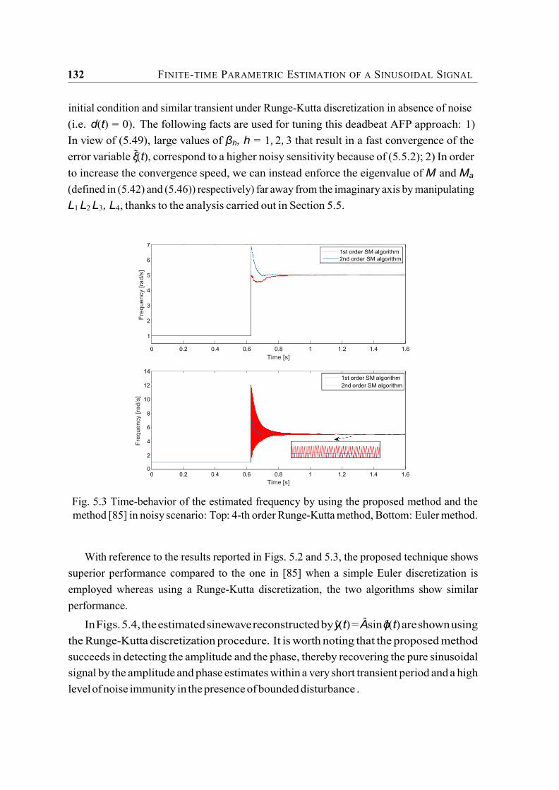
132 FINITE-TIME PARAMETRIC ESTIMATION OF A SINUSOIDAL SIGNAL
initial condition and similar transient under Runge-Kutta discretization in absence of noise
(i.e. d(t) = 0). The following facts are used for tuning this deadbeat AFP approach: 1)
In view of (5.49), large values of βh, h = 1, 2, 3 that result in a fast convergence of the
error variable ξ(t), correspond to a higher noisy sensitivity because of (5.5.2); 2) In order
to increase the convergence speed, we can instead enforce the eigenvalue of M and Ma
(defined in (5.42) and (5.46)) respectively) far away from the imaginary axis by manipulating
L1 L2 L3, L4, thanks to the analysis carried out in Section 5.5.
0 0.2 0.4 0.6 0.8 1 1.2 1.4 1.6
Time [s]
14
1st order SM algorithm
12 2nd order SM algorithm
10
8
6
4
2
0
0 0.2 0.4 0.6 0.8 1 1.2 1.4 1.6
Time [s]
Fig. 5.3 Time-behavior of the estimated frequency by using the proposed method and the
method [85] in noisy scenario: Top: 4-th order Runge-Kutta method, Bottom: Euler method.
With reference to the results reported in Figs. 5.2 and 5.3, the proposed technique shows
superior performance compared to the one in [85] when a simple Euler discretization is
employed whereas using a Runge-Kutta discretization, the two algorithms show similar
performance.
In Figs. 5.4, the estimated sinewave reconstructed by y(t) = A sin ϕ(t) are shown using
the Runge-Kutta discretization procedure. It is worth noting that the proposed method
succeeds in detecting the amplitude and the phase, thereby recovering the pure sinusoidal
signal by the amplitude and phase estimates within a very short transient period and a high
level of noise immunity in the presence of bounded disturbance .
7
6
1st order SM algorithm
2nd order SM algorithm
5
4
3
2
1
Fre
qu
en
cy [
rad
/s]
Fre
que
ncy [ra
d/s
]

5.7 Simulation results 133
5
4
3
2
1
0
-1
-2
-3 0 0.2 0.4 0.6 0.8 1 1.2 1.4 1.6 1.8 2
Time [s]
6
4
2
0
-2
-4 0 0.2 0.4 0.6 0.8 1 1.2 1.4 1.6 1.8 2
Time [s]
Fig. 5.4 Time-behavior of the reconstructed pure sine-wave by using the proposed method in
noise-free and noisy scenarios.
Example 2: In this second more challenging example, the behavior of the proposed
method is compared with the modulating function-based estimator proposed in [33] and the
first order sliding mode approach [85].
Consider a biased and noisy sinusoidal signal
v(t) = A0(t) + A(t) sin(2πf (t) t) + d(t),
where the amplitude, frequency and the offset change over time according to the follow-
ing pattern: A(t) = 10, f (t) = 50Hz, A0(t) = 1, 0 ≤ t < 0.5, A(t) = 12, f (t) =
52Hz, A0(t) = 0.8, 0.5 ≤ t < 1. d(t) is a signal with uniform distribution in the interval
[−0.5, 0.5]. The parameters of the method in [33] are set as T = π/10, n = 500, µ =
0.99, K = 6. Method [85] implements three kernels having parameters: β1 = 50, β2 =
80, β3 = 100, β = 60, while g = 30, L = 1.2 × 10⁶. The proposed method is equipped
with the same kernels as the 1-st order SM algorithm [85], whereas g = 30, ga = 100, L1 =
2 × 10⁴, L2 = 20, L3 = 1 × 10⁵ and L4 = 50.
In principle, the method given in [33] identifies the true frequency “instantaneously" as
it is enabled, whereas the proposed method achieves finite-time convergence with tunable
convergence rate determined by the parameter L1, L2. It is worth noting from Fig. 5.5 that
biased input unbiased input estimated sinusoid
biased input unbiased input estimated sinusoid
Sig
na
l S
ign
al

134 FINITE-TIME PARAMETRIC ESTIMATION OF A SINUSOIDAL SIGNAL
54
Volterra method with FOSM adaptation [32]
Modulation function method [31] 53 Volterra method with SOSM adaptation
52
51
50
49
48
0 0.1 0.2 0.3 0.4 0.5 0.6 0.7 0.8 0.9 1
Time [s]
Fig. 5.5 Time-behavior of the estimated frequency by using the proposed method (blue line)
compared with the time behaviors of the estimated frequency by the finite-time method [33]
(red line) and the 1-st order SM method [85] (green line) respectively.
they are tuned with similar response to the initial frequency and the same initial condition
f(0) = 48Hz for fair comparison. Although all the methods deal with the frequency
step in a very fast manner, the proposed estimator performs slightly better in terms of
robustness against bounded disturbances. Indeed, the chattering phenomenon in steady state
is significantly mitigated by using a higher order sliding mode adaptation scheme.
Example 3: In this example, a comparison concerning the frequency estimation is carried
out between the presented method and a recently proposed method [79] also addressing
finite-time frequency estimation. Consider the biased signal used in the example reported in
[79]
y(t) = 2 + 3 sin(4t + π/4) (5.55)
with unknown sinusoidal parameters. The adaptation law of method [79] is initialized
by Θ 1(0) = [0, 0, 0]⊤, while the learning gain and other coefficients are set as Γ1 =
diag([50, 500, 500]), λ1 = 2.5, λ2 = 5, l = 1, κ = 0.001. On the other hand, the pro-
posed method is tuned by β1 = 1, β2 = 2, β3 = 3, β = 2.5, g = 3, L1 = 30, L2 = 2, δϵ =
1 × 10⁻⁴ and the same initial frequency estimate ω(0) = √
5. The behavior of both methods
is shown in a noise-free scenario and in the case of noisy measurements where the noise has
the same characteristics as in the previous example (see Fig. 5.6). As can be noticed, the
proposed method compares favorably with the one in [79].
Unlike the algorithm illustrated in [79] where the (unknown) initial conditions of the
signal generators’ state significantly affect the estimates during the transient, the proposed
Fre
que
ncy [
Hz]

5.8 Concluding Remarks 135
Fre
qu
en
cy [
rad
/s]
Fre
qu
en
cy [
rad
/s]
4.5
Estimated frequency in noisy-free condition
4
3.5
3
2.5
2
1.5
1
0.5
0 0 1 2 3 4 5 6 7 8 9 10
Time [s]
Estimated freqyency in presence of noise-u.d. [-0.5,0.5] 6
5
4
3
2
1 Recent method on Automatica
Proposed method
0
0 1 2 3 4 5 6 7 8 9 10 Time [s]
Fig. 5.6 Time-behavior of the estimated frequency by using the proposed method (blue line)
compared with the time behaviors of the estimated frequency obtained by the method [79]
(red line) respectively. Top: noise-free case. Bottom: noisy case.
estimation methodology inherently annihilates the initial conditions. To enhance this signif-
icant feature, in Fig. 5.6 two simulations referred to different initial conditions but using
the same input signal (5.55) are reported. As can be noticed, the proposed method yields in
finite-time the same estimate of the frequency, irrespective of the initial conditions.
5.8 Concluding Remarks
In the this chapter, the problem of AFP identification from a noisy and biased measure-
ment has been addressed. With the aim of addressing the challenging issue, we introduce a
novel deadbeat estimator, which can provide reliable frequency estimates within an arbitrary
small finite time. The method consists in processing the measured signal with Volterra opera-
tors, to obtain auxiliary signals that are used in combination with second-order sliding mode
adaptation laws to estimate the frequency, the amplitude and the phase of the original signal.
This algorithm has been proved to be finite-time convergent in nominal condition and enjoys
Recent method on Automatica
Proposed method

136 FINITE-TIME PARAMETRIC ESTIMATION OF A SINUSOIDAL SIGNAL
Fre
qu
en
cy [
rad
/s]
Fre
qu
ency [
rad/s
]
Estimated frequency with different initial conditions in noisy free scenario (method from Automatica)
4
3.5
3
2.5
2
1.5
1
0.5
0 0 1 2 3 4 5 6 7 8 9 10
Time [s]
4.5
Estimated frequency with different initial conditions in noisy free scenario (proposed method)
4
3.5
3
2.5
2
1.5
0 1 2 3 4 5 6 7 8 9 10 Time [s]
Fig. 5.7 Time-behavior of the estimated frequency with different initial conditions and in a
noise-free scenario. Left: the estimator proposed in [79]. Right: the proposed method.
ISS stability properties with respect to bounded measurement perturbations. Numerical
examples have been reported showing the effectiveness of the proposed method compared to
recently published results.

Chapter 6
CONCLUSIONS AND FUTURE
PROSPECTS
6.1 Concluding Remarks
Parameter estimation of a sinusoidal signal perturbed by additive disturbances has been
accomplished by a wide variety of techniques in the literature including extended Kalman
filters, phase locked loop tools, adaptive notch filtering and internal model based techniques.
This thesis first of all provides a thorough review of the literature with special emphasis
on several representative approaches, such as KF, PLL, ANF, SVF and AO, which are all
characterized by asymptotic convergence. On the other hand, AFP estimators that can
converge within a (possibly very small) finite time represent a special category that is seldom
discussed and solved so far. The available methods are mainly devised by two strategies:
algebraic derivative and modulating functions, whereas there is a lack of the theoretical
investigation for the convergence properties in the presence of bounded measurement noise.
Besides, as mentioned in Chapter 1.3 research challenges also consist in other aspects (e.g.,
global stability, accuracy, multi-frequency estimation), which are studied herein.
In this thesis, the problem of adaptive estimation of the characteristics of a single sinu-
soidal signal from a measurement affected by structured and unstructured disturbances is
addressed. Thanks to the proposed pre-filtering technique, the structured disturbances that
belong to a class of time-polynomial signals incorporating both bias and drift phenomena
can be tackled in a unified manner. We basically propose two asymptotic methods designed
respectively by adaptive observer and state variable filtering tools. In the estimation context
presented in the thesis, the “instantaneous” persistency of excitation condition is embedded in
the proposed algorithms rather than the standard “integral” type PE condition. This is a very

138 CONCLUSIONS AND FUTURE PROSPECTS
significant feature in terms of on-line implementation, since it makes it possible to enhance
the performance when the system is weakly excited resorting a typical excitation-based
switching algorithm without the need for on-line approximate computation of integrals. The
stability of the devised AFP systems are analyzed by an ISS analysis, whereby we induce a
few tuning guidelines for the adjustable parameters of the proposed algorithms, depending on
the assumed noise level and on the required asymptotic accuracy. More specifically, the AO
scheme has been shown robust even in the presence of multi-harmonics, while the ISS bound
depends on the power of the total harmonic contents. The SVF approach provides advantages
in terms of implementation due to the reduced complexity. From a practical perspective, the
discretized algorithm is subject to a steady-state bias, motivated by which a post-correction
formula is devised for the compensation under Euler discretization method.
The AO system for a single sine wave has also been extended into a generic structure
for estimating amplitudes, frequencies and phases of biased multi-sinusoidal signals in the
presence of bounded perturbations on the measurement. The key aspect of advantages over
existing tools is the realization of direct detection of the unknown frequencies with ISS
stability guarantee. On the other hand, thanks to the individual excitation-based switching
logic embedded in the update laws regarding each frequency component, the problem of
overparametrization is addressed.
Finally, a novel finite-time convergent estimation technique is proposed for AFP identi-
fication of a single sinusoidal signal. Resorting to Volterra integral operators with suitably
designed kernels, the measured signal is processed, yielding a set of auxiliary signals, in
which the influence of the unknown initial conditions is removed. A second-order sliding
mode-based adaptation law–fed by the aforementioned auxiliary signals–is designed for
finite-time estimation of the frequency, amplitude, and phase. The main contribution lies
in the characterization of the worst case behavior in the presence of the bounded additive
disturbances by ISS arguments.
The effectiveness of the proposed estimation approaches has been examined and com-
pared with other existing tools via extensive numerical simulations. Experimental results are
provided as well for the sake of evaluation in real-time.
6.2 Future Work
This section is devoted to highlight possible extensions of the presented methodologies.
These extensions can be explored in two directions: more comprehensive theory and possible
applications. From a theoretical point of view, the robustness characterization carried out so
far only accounts for the measurements corrupted by bounded disturbances. Future research

6.2 Future Work 139
efforts could be devoted to a probabilistic analysis of the algorithms with respect to white
and colored noises with the aim of establishing a relationship between the accuracy and
signal-to-noise ratio (SNR). Moreover, it is worth to establish the discrete-time counterparts
of the devised algorithms in an entire discrete-time framework, so that we can avoid problems
due to discretization (e.g., discretization error in state state, performance discrepancy due
to distinct discretization policy). In the context of deadbeat AFP estimation, future work
includes the design of novel kernels as well as the comparative analysis in terms of few
aspects, such as robustness, tuning of weighting factors and complexity. This may lead to the
evaluation in some real-world scenarios.
Concerning the potential application of the proposed techniques, two main research
directions can be pursued in the future: output regulation of a linear or nonlinear system
and condition (vibration) monitoring of mechanical systems. More specifically, in many
practical situations, the frequencies of the external signals are not precisely available, for
example, the periodic disturbances in rotational machinery. In this respect, it turns out that an
adaptive learning scheme for updating the profiles of unknown sinusoidal or periodic signals
is a premise of disturbance cancellation strategies, thus motivating us to embed the proposed
estimators in regulators, such as internal model principle and feedforward compensator.
On the other hand, the process of oscillations of a machine in operation is described by
mechanical vibrations, which reflect the condition of the system. A typical example is a ball
bearing that is a type of rolling-element bearing widely used in various of machinery. The
healthy monitoring of a ball bearing system consists in identifying the bearing faults induced
by different factors, such as excessive loads, over heating and corrosion. The cornerstone
behind this idea is the vibration analysis based on the on-line frequency detection that can be
dealt with by the multi-sinusoidal estimator. Finally, in the specific applications that require
the estimates to converge in a neighborhood of the true values within a predetermined finite
time, independently from the unknown initial conditions, the deadbeat AFP estimator may
turns out to be very useful by providing nearly instantaneous estimates.


References
[1] Aranovskii, S. V., Bobtsov, A. A., Kremlev, A. S., and Luk’yanova, G. V. (2007). A
robust algorithm for identification of the frequency of a sinusoidal signal. Journal of Computer and Systems Sciences International, 46(3):371–376.
[2] Aranovskiy, S., Bobtsov, A., Kremlev, A., Nikolaev, N., and O.Slita (2010). Identification of frequency of biased harmonic signal. European J. Control, 2:129–139.
[3] Best, R. E. (1999). Phase-Locked Loops, Design, Simulation, and Applications. New York: McGraw-Hill, 4th edition.
[4] Bhat, S. P. and Bernstein, D. S. (2000). Finite-time stability of continuous autonomous systems. SIAM J. Control Optim., 38(3):751–766.
[5] Bittanti, S., Campi, M., and Savaresi, S. (1997). Unbiased estimation of a sinusoid in colored noise via adapted notch filters. Automatica, 33(2):209–215.
[6] Bittanti, S. and Savaresi, S. (2000). On the parametrization and design of an extended kalman filter frequency tracker. IEEE Trans. on Automatic Control, 45(9):1718–1724.
[7] Bobtsov, A. A. (2008). New approach to the problem of globally convergent frequency estimator. Int. J. of Adaptive Control and Signal Processing, 22(3):306–317.
[8] Bobtsov, A. A., Efimov, D., Pyrkin, A. A., and Zolghadri, A. (2012). Switched algo- rithm for frequency estimation with noise rejection. IEEE Trans. on Automatic Control, 57(9):2400–2404.
[9] Bodson, M. and Douglas, S. (1997). Adaptive algorithms for the rejection of sinusoidal disturbances with unknown frequency. Automatica, 33(12):2213–2221.
[10] Bodson, M., Jensen, J. S., and Douglas, S. C. (2011). Active noise control for periodic disturbances. IEEE Trans. on Control System Technology, 9(1):200–205.
[11] Bollen, M. (2011). The Smart Grid: Adapting the power system to new challenges (Synthesis Lectures on Power Electronics). Morgan and Claypool Publishers.
[12] Brown, L. J. and Zhang, Q. (2003). Identification of periodic signals with uncertain frequency. IEEE Trans. on Signal Processing, 51(6):1538–1545.
[13] Brown, L. J. and Zhang, Q. (2004). Periodic disturbance cancellation with uncertain frequency. Automatica, 40(4):631–637.
[14] Burton, T. (2005). Volterra Integral and Differential Equations. Elsevier.

142 References
[15] Carnevale, D. and A.Astolfi (2008). A minimal dimension observer for global frequency estimation. In Proc. IEEE American Control Conference, pages 5269–5274, Seattle, WA.
[16] Carnevale, D. and Astolfi, A. (2009). Hybrid observer for global frequency estimation of saturated signals. IEEE Trans. on Automatic Control, 54(10):2461–2464.
[17] Carnevale, D. and Astolfi, A. (2011). A hybrid observer for frequency estimation of saturated multi-frequency signals. In Proc. of the IEEE Conf. on Decision and Control and European Control Conference, pages 2577–2582, Orlando, FL, USA.
[18] Carnevale, D., Galeani, S., and A.Astolfi (2010). Hybrid observer for multi-frequency signals. In Proc.of IFAC workshop Adaptation and Learning in Control and Signal Processing (ALCOSP), Bogazici University, Turkey.
[19] Chen, B., Pin, G., Ng, W. M., Hui, S. Y. R., and Parisini, T. (2015a). A parallel prefiltering approach for the identification of a biased sinusoidal signal: Theory and experiments. Int. J. Adapt. Control Signal Process.
[20] Chen, B., Pin, G., Ng, W. M., Lee, C. K., Hui, S. Y. R., and Parisini, T. (2014a). An adap- tive observer-based switched methodology for the identification of a perturbed sinusoidal signal: Theory and experiments. IEEE Trans. on Signal Processing, 62(24):6355–6365.
[21] Chen, B., Pin, G., and Parisini, T. (2013). Adaptive observer-based sinusoid identifi- cation: structured and bounded unstructured measurement disturbances. In Proc. of the IEEE European Control Conference, pages 2645–2650, Zurich, Switzerland.
[22] Chen, B., Pin, G., and Parisini, T. (2014b). An adaptive observer-based estimator for multi-sinusoidal signals. In Proc. IEEE American Control Conference, Portland, OR, USA.
[23] Chen, B., Pin, G., and Parisini, T. (2014c). Robust parametric estimation of biased sinusoidal signals: a parallel pre-filtering approach. In Proc. of the IEEE Conf. on Decision and Control, Los Angeles.
[24] Chen, B., Pin, G., and Parisini, T. (2015b). Frequency estimation of periodic signals: an adaptive observer approach. In Proc. IEEE American Control Conference, Chicago, IL, USA.
[25] de Souza Ribeiro, L., Saavedra, O., de Lima, S., and de Matos, J. (2011). Isolated micro- grids with renewable hybrid generation: The case of lencois island. IEEE Transactions on Sustainable Energy, 20(1):1–11.
[26] Delille, G., Francois, B., and Malarange, G. (2012). Dynamic frequency control support by energy storage to reduce the impact of wind and solar generation on isolated power system’s inertia. IEEE Transactions on Sustainable Energy, 3(4):931–939.
[27] D.L., M.-V., Rodriguez-Angeles, A., and Sira-Ramirez, H. (10-13 Jan. 2009). Robust gpi observer under noisy measurements. Electrical Engineering, Computing Science and Automatic Control, CCE 2009 6th International Converence, pages 1–5.
References 143
[28] Fedele, G. and Ferrise, A. (2012). Non adaptive second order generalized integrator for identification of a biased sinusoidal signal. IEEE Trans. on Automatic Control, 57(7):1838– 1842.
[29] Fedele, G. and Ferrise, A. (2014). A frequency-locked-loop filter for biased multi- sinusoidal estimation. IEEE Trans. on Signal Processing, 62(5):1125–1134.
[30] Fedele, G., Ferrise, A., and Frascino, D. (2009a). Multi-sinusoidal signal estimation by an adaptive sogi-filters bank. In 15th IFAC Symposium on System Identification, pages 402–407.
[31] Fedele, G., Ferrise, A., and Muraca, P. (2011). An adaptive quasi-notch filter for a biased sinusoidal signal estimation. In IEEE International Conference on Control and Automation (ICCA), pages 1060–1065, Santiago.
[32] Fedele, G., Ferrise, A., and Muraca, P. (2014). An adaptive “quasi” repetitive controller for the fundamental frequency estimation of periodic signals. In 19th World Congress the International Federation of Automatic Control, pages 12098–12103.
[33] Fedele, G. and L.Coluccio (2010). A recursive scheme for frequency estimation using the modulating function method. Applied Mathematics and Computation , 216(5):1393– 1400.
[34] Fedele, G., Picardi, C., and Sgro, D. (2009b). A power electrical signal tracking strategy based on the modulating functions method. IEEE Transactions on Industrial Electronics, 56(10):4079–4087.
[35] Feola, L., Langella, R., and Testa, A. (2013). On the effects of unbalances, harmonics and interarmonics in pll systems. IEEE Trans. on Instrum. and Meas., 62(9):2399–2409.
[36] Filippov, A. F. (1988). Differential equations with discontinuous right-hand sides. Dordrecht, Boston, London: Kluwer Academic Publishers.
[37] Francis, B. and Wonham, B. (1976). The internal model principle of control theory. Automatica, 12(5):457–465.
[38] Francis, B. and Wonham, W. (1975). The internal model principle for linear multivari- able regulators. Applied Mathematics and Optimization, 2:170–194.
[39] Fu, H. and Kam, P. Y. (2007). Map/ml estimation of the frequency and phase of a single sinusoid in noise. IEEE Trans. on Signal Processing, 55(3):834–845.
[40] Furthmüller, C., Colaneri, P., and Re, L. D. (2012). Adaptive robust stabilization of continuous casting. Automatica, 48(1):225–232.
[41] Gardner, F. (2005). Phaselock Techniques. New York/Oxford: Wiley Blackwell.
[42] Goebel, R. and Teel, A. R. (2006). Solutions to hybrid inclusions via set and graphical convergence with stability theory applications. Automatica, pages 573–587.
[43] Guo, X. and Bodson, M. (2003). Frequency estimation and tracking of multiple sinusoidal components. In Proc. of the IEEE Conf. on Decision and Control, Maui, Hawaii, USA.
144 References
[44] Hajimolahoseini, H., Taban, M. R., and Soltanian-Zadeh, H. (2012). Extended kalman filter frequency tracker for nonstationary harmonic signals. Measurement, 45(1):126–132.
[45] Hou, M. (2005). Amplitude and frequency estimation of a sinusoid. IEEE Trans. on Automatic Control, 50(6):855–858.
[46] Hou, M. (2007). Estimation of sinusoidal frequencies and amplitudes using adaptive identifier and observer. IEEE Trans. on Automatic Control, 52(3):493–499.
[47] Hou, M. (2012). Parameter identification of sinusoids. IEEE Trans. on Automatic Control, 57(2):467–472.
[48] Hsieh, G. C. and Hung, J. C. (1996). Phase-locked loop techniques-a survey. IEEE Trans. on Industrial Electronics, 43(6):609–615.
[49] Hsu, L., Ortega, R., and Damm, G. (1999). A globally convergent frequency estimator. IEEE Trans. on Automatic Control, 44(4):698–713.
[50] Huang, C. H., Ch.H. Lee, K. S., and Wang, Y. (2008). Frequency estimation of distorted power system signals using a robust algorithm. IEEE Trans. on Power Delivery, 23(1):41–51.
[51] Ioannou, P. and Fidan, B. (2006). Adaptive Control Tutorial. SIAM, Boston, MA.
[52] Ioannou, P. and Sun, J. (1996). Robust Adaptive Control. Pretice Hall, Boston, MA.
[53] Karimi, H., Karimi-Ghartemani, M., and Iravani, M. R. (2004). Estimation of frequency and its rate of change for applications in power systems. IEEE Trans. on Power Delivery, 19(2):472–480.
[54] Karimi-Ghartemani, M. and Iravani, M. R. (2002). A nonlinear adaptive filter for online signal analysis in power systems: Applications. IEEE Trans. on Power Delivery, 17(2):617–622.
[55] Karimi-Ghartemani, M. and Iravani, M. R. (2005). Measurement of harmonics/inter- harmonics of time-varying frequencies. IEEE Trans. on Power Delivery, 20(1):23–31.
[56] Karimi-Ghartemani, M., Karimi, H., and Bakhshai, A. R. (2009). A filtering technique for three-phase power systems. IEEE Trans. on Instrum. and Meas., 58(2):389–396.
[57] Karimi-Ghartemani, M., Karimi, H., and Iravani, M. R. (2004a). A magnitude/phase- locked loop system based on estimation of frequency and in-phase/quadrature-phase amplitudes. IEEE Trans. on Industrial Electronics, 51(2):511–517.
[58] Karimi-Ghartemani, M., Khajehoddin, S. A., Jain, P. K., Bakhshai, A., and Mojiri, M. (2012). Addressing dc component in pll and notch filter algorithms. IEEE Trans. on Power Electronics, 27(1):78–86.
[59] Karimi-Ghartemani, M., Mokhtari, H., and Iravani, M. R. (2000). Wavelet based on-line disturbance detection for power quality applications. IEEE Trans. on Power Delivery, 15(4):1212–1220.
References 145
[60] Karimi-Ghartemani, M., Mokhtari, H., Iravani, M. R., and Sedighy, M. (2004b). A signal processing system for extraction of harmonics and reactive current of single-phase systems. IEEE Trans. on Power Delivery, 19(3):979–986.
[61] Karimi-Ghartemani, M. and Ziarani, A. K. (2003). Periodic orbit analysis of two dynam- ical systems for electrical engineering applications. Journal of Engineering Mathematics, 45(2):135–154.
[62] Karimi-Ghartemani, M. and Ziarani, A. K. (2004). A nonlinear time-frequency analysis method. IEEE Trans. on Signal Processing, 52(6):1585–1595.
[63] Khalil, H. (2001). Nonlinear Systems. Prentice Hall.
[64] Kim, S. and Y.Park (1999). Active control of multi-tonal noise with reference generator based on on-line frequency estimator. Journal of Sound and Vibration, 227(3):646–666.
[65] Liu, D., Gibaru, O., and Perruquetti, W. (2011). Parameters estimation of a noisy sinusoidal signal with time-varying amplitude. In Proc. 19th Mediterranean conference on Control and automation (MED’11), pages 570 – 575, Corfu.
[66] Luviano-Juarez, A., Cortes-Romero, J., and Sira-Ramirez, H. (2015). Parameter identification of a discretized biased noisy sinusoidal signal. Measurement, 60:129–138.
[67] Marino, R. and P.Tomei (2002). Global estimation of n unknown frequencies. IEEE Trans. on Automatic Control, 47(8):1324–1328.
[68] Marino, R., Santosuosso, G. L., and Tomei, P. (2003). Robust adaptive compensation of biased sinusoidal disturbances with unknown frequency. Automatica, 39:1755–1761.
[69] Marino, R. and Tomei, P. (2014). Frequency estimation of periodic signals. In Proc. of the IEEE European Control Conference, Strasbourg.
[70] Mark, J. G., Steele, J. R., and Hansen, C. C. (1982). Residual mode phase locked loop. U.S. Patent.
[71] Mojiri, M. and Bakhshai, A. (2007a). Stability analysis of periodic orbit of an adaptive notch filter for frequency estimation of a periodic signal. Automatica, 43(3):450–455.
[72] Mojiri, M. and Bakhshai, A. R. (2004). An adaptive notch filter for frequency estimation of a periodic signal. IEEE Trans. on Automatic Control, 49(2):314–318.
[73] Mojiri, M. and Bakhshai, A. R. (2007b). Estimation of n frequencies using adaptive notch filter. IEEE Trans. on Circuits and Systems-II, 54(4):338–342.
[74] Mojiri, M., Karimi-Ghartemani, M., and Bakhshai, A. (2007a). Estimation of power system frequency using an adaptive notch filter. IEEE Trans. on Instrum. and Meas., 56(6):2470–2477.
[75] Mojiri, M., Karimi-Ghartemani, M., and Bakhshai, A. (2007b). Time-domain signal analysis using adaptive notch filter. IEEE Trans. on Signal Processing, 55(1):85–93.

146 References
[76] Mojiri, M., Karimi-Ghartemani, M., and Bakhshai, A. (2010a). Processing of harmonics and interharmonics using an adaptive notch filter. IEEE Trans. on Power Delivery, 25(2):534–542.
[77] Mojiri, M., Yazdani, D., and Bakhshai, A. (2010b). Robust adaptive frequency estima- tion of three-phase power systems. IEEE Trans. on Instrum. and Meas., 59(7):1793–1802.
[78] Moreno, J. A. and Osorio, M. (2012). Strict lyapunov functions for the super-twisting algorithm. IEEE Trans. on Automatic Control, 57(4):1035–1040.
[79] Na, J., Yang, J., Wu, X., and Guo, Y. (2015). Robust adaptive parameter estimation of sinusoidal signals. Automatica, 53:376–384.
[80] Obregon-Pulido, G., Castillo-Toledo, B., and Loukianov, A. (2002). A globally conver- gent estimator for n-frequencies. IEEE Trans. on Automatic Control, 47(5):857–863.
[81] Pei, S.-C. and Chien-ChengTseng (1994). Real time cascade adaptive notch filter scheme for sinusoidal parameter estimation. Signal Processing, 39(1-2):117–130.
[82] Pin, G. (2010). A direct approach for the frequency-adaptive feedforward cancellation of harmonic disturbances. IEEE Trans. on Signal Processing, 58(7):3513–3530.
[83] Pin, G., Assalone, A., Lovera, M., and Parisini, T. (2015 (to appear)). Non-asymptotic kernel-based parametric estimation of continuous-time linear systems. IEEE Trans. on Automatic Control.
[84] Pin, G., Chen, B., and Parisini, T. (2013a). A nonlinear adaptive observer with excitation- based switching. In Proc. of the 52nd Conference on Decision and Control, pages 4391–4398, Florence.
[85] Pin, G., Chen, B., and Parisini, T. (2015). Deadbeat kernel-based frequency estimation of a biased sinusoidal signal. In Proc. of the IEEE European Control Conference, Linz.
[86] Pin, G., Chen, B., Parisini, T., and Bodson, M. (2014). Robust sinusoid identification with structured and unstructured measurement uncertainties. IEEE Trans. on Automatic Control, 59(6):1588–1593.
[87] Pin, G., Lovera, M., Assalone, A., and Parisini, T. (2013b). Kernel-based non- asymptotic state estimation for linear continuous-time system. In Proc. of the IEEE American Control Conference, pages 3123 – 3128, Washing, DC.
[88] Pin, G. and Parisini, T. (2011). A direct adaptive method for discriminating sinusoidal components with nearby frequencies. In Proc. of the IEEE American Control Conference, pages 2994–2999, O’Farrell Street, San Francisco, CA, USA.
[89] Pin, G., Parisini, T., and Bodson, M. (2011). Robust parametric identification of sinusoisal signals: an input-to-state stability approach. In Proc. of the IEEE Conf. on Decision and Control, pages 6104–6109, Orlando, FL.
[90] Pyrkin, A. A., Bobtsov, A. A., Efimov, D., and Zolghadri, A. (2011). Frequency estimation for periodical signal with noise in finite time. In Proc. of the IEEE Conf. on Decision and Control, pages 3646–3651, Orlando, FL.
References 147
[91] Ramos, P. M. and Serra, A. C. (2009). Comparison of frequency estimation algorithms for power quality assessment. Measurement, 42:1312–1317.
[92] Regalia, P. (1991). An improved lattice-based adaptive iir notch filter. IEEE Trans. on Signal Processing, 39(9):2124–2128.
[93] Regalia, P. A. (2010). A complex adaptive notch filter. IEEE Signal Processing Letters, 17(11):937–940.
[94] Rodríguez, P., J. Pou, J. B., Candela, J. I., Burgos, R. P., and Boroyevich, D. (2007). Decoupled double synchronous reference frame pll for power converters control. IEEE Trans. on Power Electronics, 22(2):584–592.
[95] Routray, A., Pradhan, A., and Rao, P. (2002). A novel kalman filter for frequency estimation of distorted signal in power systems. IEEE Trans. on Instrum. and Meas., 51(3):469–479.
[96] Sastry, S. and Bodson, M. (1994). Adaptive Control: Stability, Convergence, and Robustness. Prentice-Hall.
[97] Scala, B. L. and Bitmead, R. (1996). Design of an extended kalman filter frequency tracker. IEEE Trans. on Signal Processing, 44(3):739–742.
[98] Scala, B. L., Bitmead, R., and James, M. R. (1995). Conditions for stability of the extended kalman filter and their application to the frequency tracking problem. Math. Control, Signals, and Syst., 8(1):1–26.
[99] Scala, B. L., Bitmead, R., and Quinn, B. (1996). An extended kalman filter frequency tracker for high-noise environments. IEEE Trans. on Signal Processing, 44(2):431–434.
[100] Sharma, B. B. and Kar, I. N. (2008). Design of asymptotically convergent frequency estimator using contraction theory. IEEE Trans. on Automatic Control, 53(8):1932–1937.
[101] Snyder, D. L. (1969). The State-Variable Approach to Continuous Estimation with Applications to Analog Communications Theory. MIT Press, Boston, MA.
[102] So, H. C., Chan, F. K. W., and Sun, W. (2011). Subspace approach for fast and accurate single-tone frequency estimation. IEEE Trans. on Signal Processing, 59(2):827–831.
[103] Stephens, D. R. (1998). Phase-Locked Loops for Wireless Communications, Digital and Analog Implementations. Dordrecht, The Netherlands: Kluwer.
[104] Tao, G. and Ioannou, P. A. (1990). Persistency of excitation and overparametrization in model reference adaptive control. IEEE Trans. on Automatic Control, 35(2):254–256.
[105] Tedesco, F., Casavola, A., and Fedele, G. (2013). Discrete-time frequency-locked-loop filters for parameters estimation of sinusoidal signals. In Proc. of the 52nd Conference on Decision and Control, pages 4399–4404, Florence.
[106] Trapero, J. R., Sira-Ramirez, H., and Battle, V. F. (2007a). An algebraic frequency estimator for a biased and noisy sinusoidal signal. Signal Processing, 87(6):1188–1201.

148 References
[107] Trapero, J. R., Sira-Ramirez, H., and Battle, V. F. (2007b). A fast on-line frequency estimator of lightly damped vibrations in flexible structures. Journal of Sound and Vibration, 307(1-2):365–378.
[108] Trapero, J. R., Sira-Ramirez, H., and Battle, V. F. (2008). On the algebraic identifica- tion of the frequencies, amplitudes and phases of two sinusoidal signals from their noisy sum. International Journal of Control, 81(3):507–518.
[109] Tsao, T., Qian, Y., and Nemani, M. (2000). Repetitive control for asymptotic tracking of periodic signals with an unknown period. J. Dyn. Syst. Meas. Contr., 122(2):364–369.
[110] Wu, B. and Bodson, M. (2003). A magnitude/phase-locked loop approach to parameter estimation of periodic signals. IEEE Trans. on Automatic Control, 48(4):612–618.
[111] Xia, X. (2002). Global frequency estimation using adaptive identifiers. IEEE Trans. on Automatic Control, 47(7):1188–1193.
[112] Yasuda, K. and Hirai, K. (1979). Upper and lower bounds on the solution of the algebraic matrix riccati and lyapunov equation. IEEE Trans. on Automatic Control, 24(6):483–487.
[113] Zhang, Q. and Brown, L. J. (2006). Noise analysis of an algorithm for uncertain frequency identification. IEEE Trans. on Automatic Control, 51(1):103–110.
[114] Zhao, L., Huang, J., Liu, H., Li, B., and Kong, W. (2014). Second-order sliding-mode observer with online parameter identification for sensorless induction motor drives. IEEE Transactions on Industrial Electronics, 61(10):5280–5289.
[115] Ziarani, A. K. and Karimi-Ghartemani, M. (2005). On the equivalence of three inde- pendently developed phase-locked loops. IEEE Trans. on Automatic Control, 50(2):2021– 2027.
[116] Ziarani, A. K. and Konrad, A. (2004). A method of extraction of nonstationary sinusoids. Signal Processing, 84(8):1323–1346.