Nonautonomous systems

Marc R. Roussel

November 1, 2005

1 Introduction

We have so far focused our attention on autonomous systems. Nonautonomous systems are ofcourse also of great interest, since systems subjected to external inputs, including of course periodicinputs, are very common.

In order to motivate our treatment of nonautonomous systems, we begin with some very simpleexamples of systems whose state spaces consist of a single variable. As we go, we will find thatnonautonomous systems are in some ways different from autonomous systems, and in other waysalike.

Example 1.1 Consider the very simple system

dxdt

= sint, (1)

with initial condition x(0) = x0. First of all, note that this system has no true equilibriumpoints: dx/dt = 0 when sint = 0, which happens when t = nπ, for any integer n. However,since t never stops changing, dx/dt is never zero for more than an instant. It is of course alsopossible to make up autonomous systems which lack equilibria (e.g. x = 1), but these oftenhave uninteresting behavior.

The state space x is no longer a proper phase space for nonautonomous differential equationsbecause the behavior at a given point in the state space depends on the time at which thatpoint was reached. Essentially, this means that the phase space is two-dimensional andconsists of the variables x and t. We can in fact formalize this by expanding our originalequation to

dxdτ

= sint (2a)

anddtdτ

= 1. (2b)

In practical terms, we haven’t gained much. Conceptually however this transformation high-lights the fact that a nonautonomous system with a d-dimensional state space is in a sense

1

xt

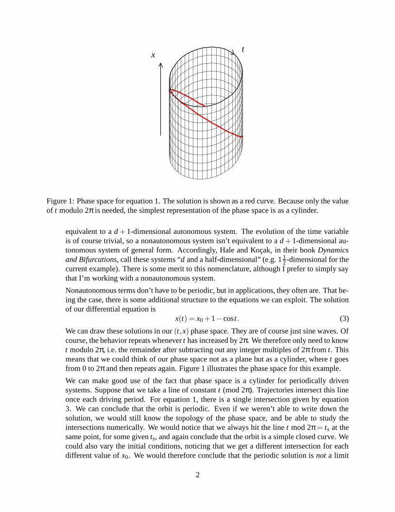
Figure 1: Phase space for equation 1. The solution is shown as a red curve. Because only the valueof t modulo 2π is needed, the simplest representation of the phase space is as a cylinder.

equivalent to a d + 1-dimensional autonomous system. The evolution of the time variableis of course trivial, so a nonautonomous system isn’t equivalent to a d + 1-dimensional au-tonomous system of general form. Accordingly, Hale and Kocak, in their book Dynamicsand Bifurcations, call these systems “d and a half-dimensional” (e.g. 1 1

2 -dimensional for thecurrent example). There is some merit to this nomenclature, although I prefer to simply saythat I’m working with a nonautonomous system.

Nonautonomous terms don’t have to be periodic, but in applications, they often are. That be-ing the case, there is some additional structure to the equations we can exploit. The solutionof our differential equation is

x(t) = x0 +1− cos t. (3)

We can draw these solutions in our (t,x) phase space. They are of course just sine waves. Ofcourse, the behavior repeats whenever t has increased by 2π. We therefore only need to knowt modulo 2π, i.e. the remainder after subtracting out any integer multiples of 2π from t. Thismeans that we could think of our phase space not as a plane but as a cylinder, where t goesfrom 0 to 2π and then repeats again. Figure 1 illustrates the phase space for this example.

We can make good use of the fact that phase space is a cylinder for periodically drivensystems. Suppose that we take a line of constant t (mod 2π). Trajectories intersect this lineonce each driving period. For equation 1, there is a single intersection given by equation3. We can conclude that the orbit is periodic. Even if we weren’t able to write down thesolution, we would still know the topology of the phase space, and be able to study theintersections numerically. We would notice that we always hit the line t mod 2π = ts at thesame point, for some given ts, and again conclude that the orbit is a simple closed curve. Wecould also vary the initial conditions, noticing that we get a different intersection for eachdifferent value of x0. We would therefore conclude that the periodic solution is not a limit

2

cycle, but is in fact some form of conservative oscillation. It turns out that system 2 is in factHamiltonian.

Describing the motion in terms of the intersections of the solution with a given line (or surface,in general) is an important technique of nonlinear dynamics. The line t mod 2π = ts is called asurface of section, or Poincare section. We will return to this idea shortly.

Example 1.2 Consider the differential equation

dxdt

= −x+ cos t,

with initial condition x = x0 at t = 0. If you happen to know the variation of constantsformula, you can solve this equation by hand, or you can just use Maple:

> dsolve({diff(x(t),t)=-x(t)+cos(t),x(0)=x0},x(t));

x(t) =12

cos(t)+12

sin(t)+ e(−t) (−12

+ x0)

Note that at long times, all solutions approach the unique solution

x(t) =12

(cos t + sin t) .

This is a limit cycle in the x × (t mod 2π) phase space: It’s a solution of the governingequation, and the general solution clearly implies that the system returns to this solution if itis displaced from it slightly.

The two foregoing examples hint that most of the behaviors which are possible in a planardynamical system are also possible in a nonautonomous system. As mentioned above, the one thingwe can’t have is a true equilibrium point, unless of course we extend our notion of equilibrium.

Example 1.3 Consider the differential equation

dxdt

= −x+1t−

1t2 .

As t → ∞, dx/dt → −x. It follows that we eventually get solutions which exponentiallydecay to zero. Since the nonautonomous term is not periodic, the phase space is now theentire (t,x) plane. In a sense, this system therefore has an equilibrium point at (+∞,0)which is reached for initial conditions with t > 0.

It is often convenient to describe equilibrium points at infinity. In some cases, we can workwith them directly as we have done here. In others, it is easier to transform to a coordinate

3

system which places these equilibria at finite coordinates. In this case, we are interested inthe planar system

dxdτ

= −x+1t−

1t2 ,

dtdτ

= 1.

We want to change our coordinate system such that the interval [0,∞) is mapped into somefinite interval, say [0,1]. There are many possible transformations, of which the following isparticularly convenient:

θ =t

t +1.

By the chain rule,

dθdτ

=dθdt

dtdτ

=1

(t +1)2 .

Also, t =θ

1−θ.

∴dθdτ

= (1−θ)2

anddxdτ

= −x+1−θ

θ−

(

1−θθ

)2

.

The point (θ∗,x∗) = (1,0) is clearly an equilibrium point of the transformed system. Thesystem is now in a form in which we can study the stability of this point, and by inferrencethe stability of the equilibrium point at infinity of the original system.

2 Poincare sections

Recall the Brusselator model:

Ak1−→X

B+Xk2−→Y+D

2X+Yk3−→ 3X

Xk4−→E

After reducing to dimensionless form, we had obtained the equations

x = a−bx+ x2y− x,

y = bx− x2y.

4

In our earlier work with this model, it was assumed that a and b were constants. Now supposeinstead that the chemical A is supplied periodically:

a = a0 +αsin(2πt/T), (4)

where T is the period of the input, and a0 and α are constants. We can’t solve these equationsanalytically. However, we can use some of the ideas developed above to study this system.

First, since the input is periodic, we work in the phase space a× b× (t mod T ). A periodicphase space of this sort is available in xpp. We use the following input file:

# Brusselator ode file

# Differential equations:x’ = a0 + alpha*sin(2*pi*theta/period) - b*x + xˆ2*y - xy’ = b*x - xˆ2*ytheta’ = 1

# Initial conditionsx(0) = 0.9y(0) = 0.9

# Default values of the parameters:param a0=1, b=3param alpha=0.01, period=1

# Reserve lots of storage space# in case we want to get a long trajectory@ MAXSTOR=1000000

done

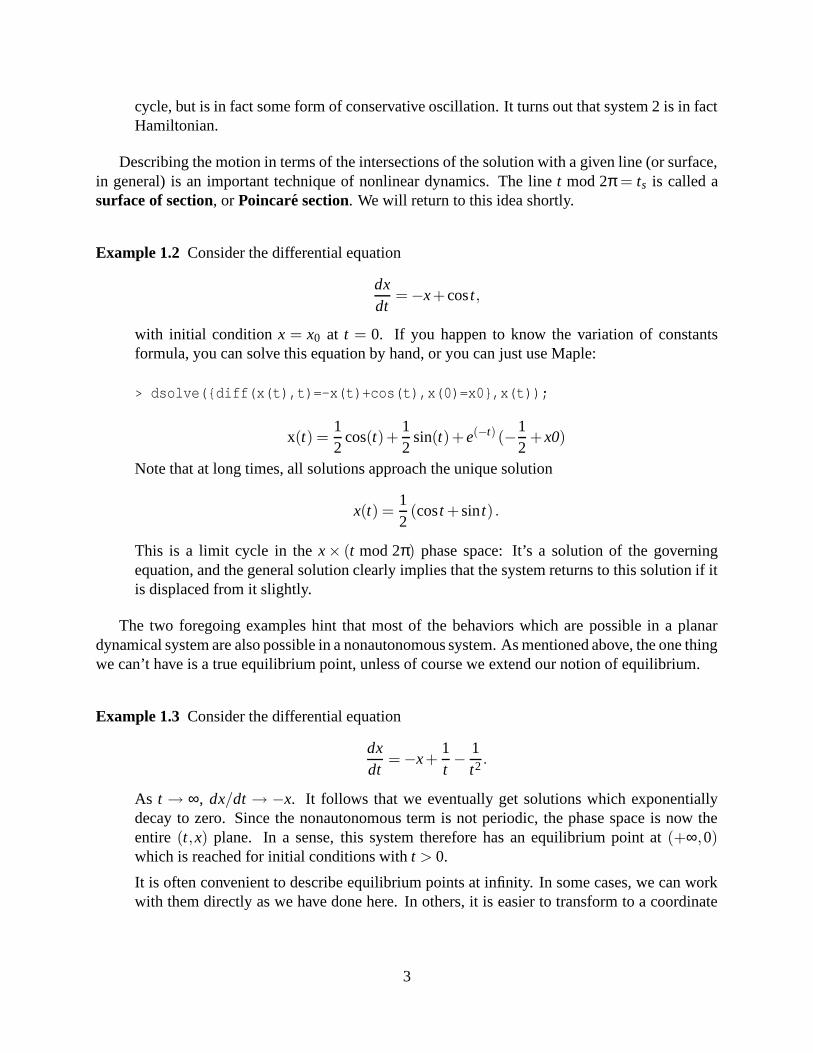
Because xpp always uses t for time, I’ve had to change our naming convention, using theta forthe time in our autonomous set. After starting xpp, click on phAsespace→Choose. Set the periodto 1, then select theta in the dialog box which appears and click on Done. Click on Viewaxesand arrange for x to be plotted vs theta. Finally, set Total to 200 and tRansient to 100 in theNumerics menu. This will give us a reasonably long trajectory while discarding any short-livedtransient behavior. If you run the model, and then click on Window/zoom→Fit, you will see asomewhat complicated picture (Fig. 2). Remember that we’re looking at trajectories on a cylinder.1

The right and left edges of the image are therefore associated. What is happening effectively is thatthe period of the system for these parameters is different from the driving period. We can confirmthis by looking at (e.g.) x vs t, which clearly shows that the system oscillates with a period of about7 time units. We have two irrationally related frequencies, so we have a quasiperiodic orbit onthe cylinder. This orbit will in time completely cover the cylinder.

We get a quasiperiodic orbit in this case because the driving is too weak and too far removedfrom the system’s natural frequency to entrain it. Change alpha to 0.5 and period to 5 in the xppparameter window. Don’t forget to also change the period in the phAsespace dialog to 5. The

1The geometry is a little more complicated than that because there’s a third variable, y, but the image of a cylinderis a useful one.

5

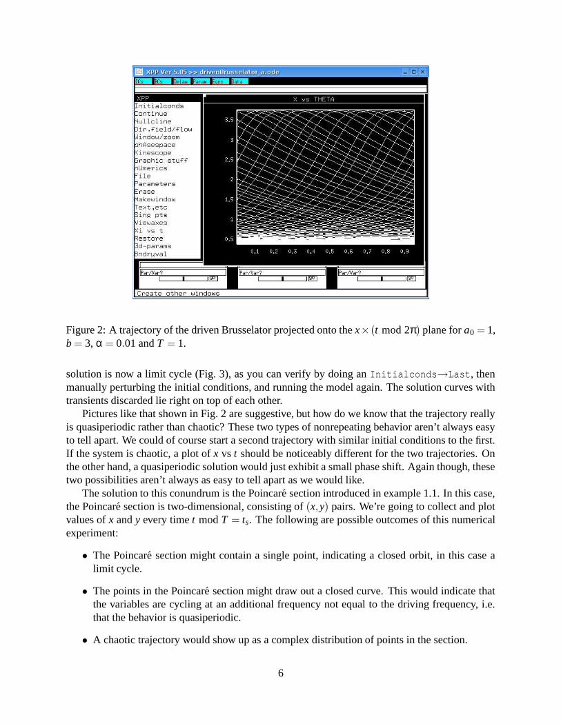
Figure 2: A trajectory of the driven Brusselator projected onto the x× (t mod 2π) plane for a0 = 1,b = 3, α = 0.01 and T = 1.

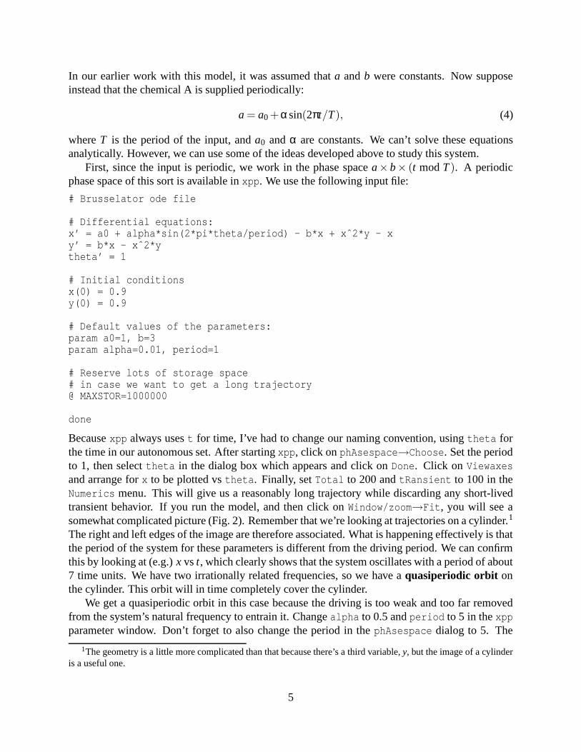
solution is now a limit cycle (Fig. 3), as you can verify by doing an Initialconds→Last, thenmanually perturbing the initial conditions, and running the model again. The solution curves withtransients discarded lie right on top of each other.

Pictures like that shown in Fig. 2 are suggestive, but how do we know that the trajectory reallyis quasiperiodic rather than chaotic? These two types of nonrepeating behavior aren’t always easyto tell apart. We could of course start a second trajectory with similar initial conditions to the first.If the system is chaotic, a plot of x vs t should be noticeably different for the two trajectories. Onthe other hand, a quasiperiodic solution would just exhibit a small phase shift. Again though, thesetwo possibilities aren’t always as easy to tell apart as we would like.

The solution to this conundrum is the Poincare section introduced in example 1.1. In this case,the Poincare section is two-dimensional, consisting of (x,y) pairs. We’re going to collect and plotvalues of x and y every time t mod T = ts. The following are possible outcomes of this numericalexperiment:

• The Poincare section might contain a single point, indicating a closed orbit, in this case alimit cycle.

• The points in the Poincare section might draw out a closed curve. This would indicate thatthe variables are cycling at an additional frequency not equal to the driving frequency, i.e.that the behavior is quasiperiodic.

• A chaotic trajectory would show up as a complex distribution of points in the section.

6

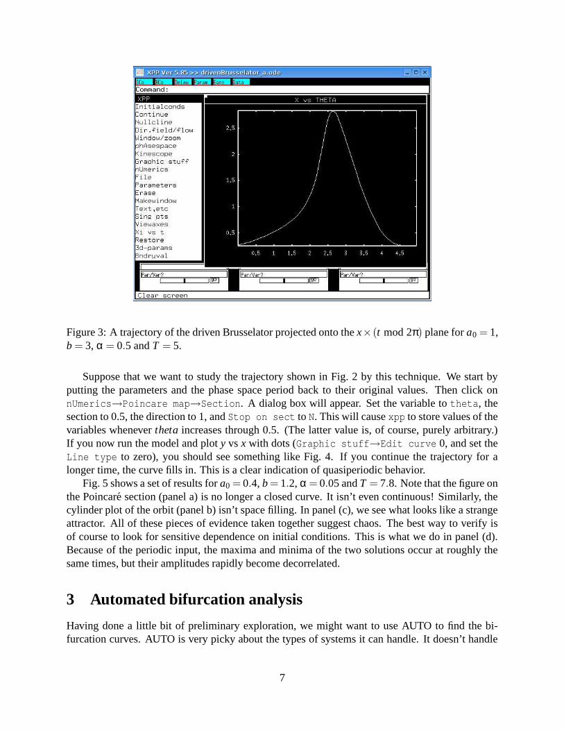
Figure 3: A trajectory of the driven Brusselator projected onto the x× (t mod 2π) plane for a0 = 1,b = 3, α = 0.5 and T = 5.

Suppose that we want to study the trajectory shown in Fig. 2 by this technique. We start byputting the parameters and the phase space period back to their original values. Then click onnUmerics→Poincare map→Section. A dialog box will appear. Set the variable to theta, thesection to 0.5, the direction to 1, and Stop on sect to N. This will cause xpp to store values of thevariables whenever theta increases through 0.5. (The latter value is, of course, purely arbitrary.)If you now run the model and plot y vs x with dots (Graphic stuff→Edit curve 0, and set theLine type to zero), you should see something like Fig. 4. If you continue the trajectory for alonger time, the curve fills in. This is a clear indication of quasiperiodic behavior.

Fig. 5 shows a set of results for a0 = 0.4, b = 1.2, α = 0.05 and T = 7.8. Note that the figure onthe Poincare section (panel a) is no longer a closed curve. It isn’t even continuous! Similarly, thecylinder plot of the orbit (panel b) isn’t space filling. In panel (c), we see what looks like a strangeattractor. All of these pieces of evidence taken together suggest chaos. The best way to verify isof course to look for sensitive dependence on initial conditions. This is what we do in panel (d).Because of the periodic input, the maxima and minima of the two solutions occur at roughly thesame times, but their amplitudes rapidly become decorrelated.

3 Automated bifurcation analysis

Having done a little bit of preliminary exploration, we might want to use AUTO to find the bi-furcation curves. AUTO is very picky about the types of systems it can handle. It doesn’t handle

7

Figure 4: Poincare section for the parameters of Fig. 2. The section was taken at t mod T = 0.5.

nonautonomous systems. It also doesn’t know anything about cylindrical phase spaces, and it’snot much use for systems in which one variable runs away to infinity, so our trick of adding adifferential equation for t won’t be of much help here.

What we need to do instead is to add differential equations whose solutions are our desirednonautonomous terms. Because we don’t really want to study the stability of these added equa-tions, our nonautonomous terms should furthermore be stable solutions of these equations. Forsinusoidal inputs, the following equations have the desired properties:

u = u(1−u2− v2)−2πv/T,

v = v(1−u2− v2)+2πu/T.

With initial conditions (u(0),v(0)) = (1,0), the solution of these equations is

(u(t),v(t)) = (cos(2πt/T),sin(2πt/T)) .

Here is an xpp input file for this extended system:

# Driven Brusselator ode file

# Differential equations:x’ = a0 + alpha*v - b*x + xˆ2*y - xy’ = b*x - xˆ2*yu’ = u*(1-uˆ2-vˆ2) - 2*pi*v/periodv’ = v*(1-uˆ2-vˆ2) + 2*pi*u/period

8

2

2.2

2.4

2.6

2.8

3

3.2

3.4

0.26 0.27 0.28 0.29 0.3 0.31 0.32 0.33 0.34 0.35 0.36

y

x

(a)

0.2

0.3

0.4

0.5

0.6

0.7

0.8

0.9

1

0 1 2 3 4 5 6 7

x

t mod T

(b)

1.6

1.8

2

2.2

2.4

2.6

2.8

3

3.2

3.4

0.2 0.3 0.4 0.5 0.6 0.7 0.8 0.9 1

y

x

(c)

0.2

0.3

0.4

0.5

0.6

0.7

0.8

0.9

1

0 50 100 150 200 250 300 350 400 450 500

x

t

(d)(0.4,2)

(0.4,2.1)

Figure 5: Some numerical integration results for the driven Brusselator with a0 = 0.4, b = 1.2,α = 0.05 and T = 7.8. Panel (a) shows a Poincare section taken at t mod T = 1 integrated for10 000 time units with a transient of 1500 time units. Panel (b) shows a trajectory on the cylindricalphase space. Panel (c) shows a trajectory in the (x,y) state space. Both of the latter were from asimulation corresponding to 3000 units of simulation time, again with a 1500 unit transient omitted.Panel (d) shows a pair of trajectories started from nearby points (noted in the legend) at t = 0.

9

# Initial conditionsx(0) = 0.9y(0) = 0.9u(0) = 1v(0) = 0

# Parameter values we want to study:param a0=0.4, b=1.2param alpha=0.5, period=7.8

# Reserve lots of storage space# in case we want to get a long trajectory@ MAXSTOR=1000000

done

We’re going to use this expanded model to study the driven Brusselator in the parameter range ofFig. 5. Note that I’ve set α = 0.5, but that all other parameters are set as in the figure.

Because of the periodic driving, we won’t be able to identify a stable steady state from which tostart AUTO.2 AUTO can also start from periodic solutions, but it’s tricky. For one thing, the wholesystem has to be expressing the same period. In other words, we can’t start from a quasiperiodicsolution. That means that we have to find a solution in which the Brusselator locks onto thedriving signal and produces a simple limit cycle in our cylindrical phase space. That’s why I chosean initial value of 0.5 for the parameter α, a value which I found using the previous xpp input fileand its cylindrical phase space. Note that this is an unphysical value for this parameter since a canthen be negative (equation 4). That doesn’t matter for our current purposes.

Once we have started xpp with our new input file, we need to integrate long enough to get rid ofany transients. We therefore run for 2000 units of simulation time, then hit Initialconds→Last.This gives us some initial conditions on the limit cycle. When studying periodic solutions, AUTOneeds an estimate of the period to be stored in the Total integration time. Because we’re startingwith a simple limit cycle, we know exactly what the period is: It’s 7.8 units. If you right-click in theplot area, xpp will print out the x and y coordinates on the screen (not to be confused with the x andy variables in this model). You can therefore read off the times corresponding to two successivemaxima or minima and verify that the period is indeed 7.8. If you set Numerics→Total to thisvalue, and then do Initialconds→Last a few times, you will find that the curves plot right ontop of each other, which confirms that the period is indeed 7.8.

It’s time to start AUTO (File→Auto). Click on Axes→Hi and fill in the values as follows:

2We could fix this by (a) modifying the equations of the (u,v) system such that they have a stable steady statefor some value of a newly introduced parameter, (b) setting b below the Andronov-Hopf bifurcation, and perhaps(c) setting α = 0.We could then follow solution branches within AUTO to get to our desired initial parameters. In thiscase though, this seems like rather a lot of work, and there is an alternative.

10

In the Numerics dialog, set Ds to −0.01, Dsmin to 0.0001, and Dsmax to 0.1. Also set Par Max to0.5. We want to follow a branch of periodic solutions, so click on Run→Periodic. AUTO findsa period-doubling bifurcation at α = 0.475. If we grab this point and ask AUTO to follow theperiod-doubling branch, it finds the following additional interesting points:

• a period-doubling point at α = 0.145,• another period-doubling point at α = 3.32×10−2, and• a torus bifurcation at α = 8.46×10−3.

(It actually finds each of these points over and over again. The small differences between the valuesof α from one pass to the other gives you an idea of how accurate these computations are. Onceyou notice this happening, you can hit the ABORT button to stop AUTO.)

If we continue to grab and run continuations on the period-doubling branches, we find thefollowing period-doubling points:

α Period4.75×10−1 7.81.45×10−1 15.69.83×10−2 31.29.05×10−2 62.44.24×10−2 31.23.32×10−2 15.6

Note that the period doubling points accumulate near α = 0.09. Presumably, there is a similaraccumulation at the low end, perhaps around α = 0.05, although I couldn’t find as many period-doubling points there as at the higher end. If I tried a bit harder (smaller values of Ds and Dsmax), Imight find a few more period-doubling points. In any event, it’s pretty clear that the chaotic regionis somewhere around values of α between 0.05 and 0.09, which is where we found it earlier (Fig.5).

There’s still the matter of exploring what the torus bifurcation does, so let’s go back to xpp.Again, our first xpp input file is most convenient for this kind of thing. This bifurcation occurs forα = 8.46×10−3, so let’s take a couple of values of α to either side of this value, say 8.4×10−3 and8.5×10−3. This turns out to be trickier than might first appear, so here’s the procedure I followed:

11

0.3

0.32

0.34

0.36

0.38

0.4

0.42

0.44

0.46

0.48

0.5

0.52

0 1 2 3 4 5 6 7

x

t mod T

(a) α=0.01α=0.009

α=0.0085

0.25

0.3

0.35

0.4

0.45

0.5

0.55

0.6

0.65

0 1 2 3 4 5 6 7

x

t mod T

(b)

0.25

0.3

0.35

0.4

0.45

0.5

0.55

0.6

0.65

0 1 2 3 4 5 6 7

x

t mod T

(c)

Figure 6: (a) Limit cycles obtained for a0 = 0.4, b = 1.2, T = 7.8 and various values of α (dis-tinguished by color). (b) Quasiperiodic solution at α = 0.0084. (c) Quasiperiodic solution atα = 0.009.

1. Start at α = 0.01 and compute the trajectory with a very long transient (5000 time units). Weget a closed orbit (Fig. 6a).

2. Decrease α to 0.009, and do an Initialconds→Last. This starts the trajectory from theperiodic orbit found for α = 0.01, which we may hope is close to the trajectory for α = 0.009.We again get a closed orbit (Fig. 6a).

3. Decrease α to 0.0085, and do Initialconds→Last again. This time, we get somethingslightly messy, so do Initialconds→Last a few more times. The problem we’re encoun-tering is called critical slowing down, which just means that the transients are longer closeto bifurcation points. We eventually recover a periodic orbit (Fig. 6a).

4. Repeat the above procedure for α = 0.0084. This time, we get a complex (quasiperiodic)orbit, no matter how many times we do Initialconds→Last (Fig. 6b).

The torus bifurcation has converted our limit cycle into a quasiperiodic solution. We can picturequasiperiodic solutions as windings around a torus. Physically, we have simply dropped the valueof α to such a low value that the periodic term is no longer strong enough to entrain the Brusse-lator, so we see both the Brusselator’s natural frequency and the driving signal’s frequency in thesolutions. Mathematically, you can picture this as a bifurcation of a closed curve into a torus.

The reason that we had to be so careful in going through this exercise is that, over a narrow

12

range of parameters, there is bistability between the torus and the limit cycle. To see this, increaseα back to 0.009 and do an Initialconds→Last from the solution computed at the smaller valueof α. A quasiperiodic solution appears (Fig. 6c). Which attractor we reach depends on the initialconditions. The lesson here is that, when doing this kind of work, it’s never a bad idea to tryapproaching the bifurcation point from both directions. You often discover interesting things thatway.

13