noname manuscript no. renato cordeiro de amorim · noname manuscript no. (will be inserted by the...
TRANSCRIPT

arX
iv:1
601.
0348
3v1
[cs.
LG]
22 S
ep 2
015
Paper accepted: Journal of Classification (Springer), expected in 2016.
Noname manuscript No.(will be inserted by the editor)
A survey on feature weighting based K-Means algorithms
Renato Cordeiro de Amorim
Received: 21 May 2014, Revised: 18 August 2015.
Abstract In a real-world data set there is always the possibility, rather high in ouropinion, that different features may have different degrees of relevance. Most ma-chine learning algorithms deal with this fact by either selecting or deselecting fea-tures in the data preprocessing phase. However, we maintainthat even among rele-vant features there may be different degrees of relevance, and this should be takeninto account during the clustering process.
With over 50 years of history, K-Means is arguably the most popular partitionalclustering algorithm there is. The first K-Means based clustering algorithm to com-pute feature weights was designed just over 30 years ago. Various such algorithmshave been designed since but there has not been, to our knowledge, a survey inte-grating empirical evidence of cluster recovery ability, common flaws, and possibledirections for future research. This paper elaborates on the concept of feature weight-ing and addresses these issues by critically analysing someof the most popular, orinnovative, feature weighting mechanisms based in K-Means.
Keywords Feature weighting· K-Means· partitional clustering· feature selection.
1 Introduction
Clustering is one of the main data-driven tools for data analysis. Given a data setYcomposed of entitiesyi ∈ Y for i = 1, 2, ...,N, clustering algorithms aim to partitionY into K clustersS = {S1,S2, ...,SK} so that the entitiesyi ∈ Sk are homogeneousand entities between clusters are heterogeneous, according to some notion of simi-larity. These algorithms address a non-trivial problem whose scale sometimes goesunnoticed. For instance, a data set containing 25 entities can have approximately
RC de AmorimDepartment of Computer Science, University of Hertfordshire, College Lane, Hatfield AL10 9AB, UK.Tel.: +44 01707 284345Fax: +44 01707 284115E-mail: [email protected]
2 Renato Cordeiro de Amorim
4.69x10¹³ different partitions ifK is set to four (Steinley 2006). Clustering has beenused to solve problems in the most diverse fields such as computer vision, text min-ing, bioinformatics, and data mining (Vedaldi and Fulkerson 2010; Steinley 2006;Jain 2010; Sturn, Quackenbush, and Trajanoski 2002; Huang et al. 2008; Gasch andEisen 2002; Mirkin 2012).
Clustering algorithms follow either a partitional or hierarchical approach to theassignment of entities to clusters. The latter produces a set of clustersS as well asa tree-like relationship between these clusters, which canbe easily visualised with adendogram. Hierarchical algorithms allow a given entityyi to be assigned to morethan one cluster inS, as long as the assignments occur at different levels in the tree.This extra information regarding the relationships between clusters comes at a con-siderable cost, leading to a time complexity ofO(N2), or evenO(N3) depending onthe actual algorithm in use (Murtagh 1984; Murtagh and Contreras 2011). Partitionalalgorithms tend to converge in less time by comparison (details in Section 2), butprovide only information about the assignment of entities to clusters. Partitional al-gorithms were originally designed to produce a set of disjoint clusters, in which anentity yi ∈ Y could be assigned to a single clusterSk ∈ S. K-Means (MacQueen1967; Ball and Hall 1967; Steinhaus 1956) is arguably the most popular of such algo-rithms (for more details see Section 2). Among the many extensions to K-Means, wehave Fuzzy C-Means (Bezdek 1981) which applies Fuzzy set theory (Zadeh 1965)to allow a given entityyi to be assigned to each cluster inS at different degrees ofmembership. However, Fuzzy C-Means introduces other issues to clustering, fallingoutside the scope of this paper.
The popularity of K-Means is rather evident. A search in scholar.google.comfor “K-Means” in May 2014 found just over 320, 000 results, the same search inMay 2015 found 442, 000 results. Adding to these impressive numbers, implementa-tions of this algorithm can be found in various software packages commonly used toanalyse data, including SPSS, MATLAB, R, and Python. However, K-Means is notwithout weaknesses. For instance, K-Means treats every single feature in a data setequally, regardless of its actual degree of relevance. Clearly, different features in thesame data set may have different degrees of relevance, a prospect we believe shouldbe supported by any good clustering algorithm. With this weakness in mind researcheffort has happened over the last 30 years to develop K-Meansbased approaches sup-porting feature weighting (more details in Section 4). Sucheffort has lead to variousdifferent approaches, but unfortunately not much guidanceon the choice of which toemploy in practical applications.
In this paper, we provide the reader with a survey of K-Means based weightingalgorithms. We find this survey to be unique because it does not simply explain someof the major approaches to feature weighting in K-Means, butalso provides empiricalevidence of their cluster recovery ability. We begin by formally introducing K-Meansand the concept of feature weighting in Sections 2 and 3, respectively. We then criti-cally analyse some of the major methods for feature weighting in K-Means in Section4. We chose to analyse those methods we believe are the most used or innovative, butsince it is impossible to analyse all existing methods we arepossibly guilty of omis-sions. The setting and results of our experiments can be found in Sections 5 and 6.

A survey on feature weighting based K-Means algorithms 3
The paper ends by presenting our conclusions and discussingcommon issues withthese algorithms that could be addressed in future research, in Section 7.
2 K-Means clustering
K-Means is arguably the most popular partitional clustering algorithm (Jain 2010;Steinley 2006; Mirkin 2012). For a given data setY, K-Means outputs a disjoint setof clustersS = {S1,S2, ...,SK}, as well as a centroidck for each clusterSk ∈ S.The centroidck is set to have the smallest sum of distances to allyi ∈ Sk, makingck a good general representation ofSk, often called a prototype. K-Means partitionsa given data setY by iteratively minimising the sum of the within-cluster distancebetween entitiesyi ∈ Y and respective centroidsck ∈ C. Minimising the equationbelow allows K-Means to show the natural structure ofY.
W(S,C) =K∑
k=1
∑
i∈Sk
∑
v∈V
(yiv − ckv)2, (1)
whereV represents the set of features used to describe eachyi ∈ Y. The algorithmused to iteratively minimise (1) may look rather simple at first, with a total of threesteps, two of which iterated until the convergence. However, this minimisation is anon-trivial problem, being NP-Hard even ifK = 2 (Aloise et al. 2009).
1. Select the values ofK entities fromY as initial centroidsc1, c2, ..., cK. SetS← ∅.2. Assign each entityyi ∈ Y to the clusterSk represented by its closest centroid. If
there are no changes inS, stop and outputS andC.3. Update each centroidck ∈ C to the centre of its clusterSk. Go to Step 2.
The K-Means criterion we show, (1), applies the squared Euclidean distance as inits original definition (MacQueen 1967; Ball and Hall 1967).The use of this particulardistance measure makes the centroid update in Step three of the algorithm aboverather straightforward. Given a clusterSk with |Sk| entities,ckv =
1|Sk|
∑
i∈Skyiv, for
eachv ∈ V.One can clearly see that K-Means has a strong relation with the Expectation Max-
imisation algorithm (Dempster, Laird, and Rubin 1977). Step two of K-Means can beseen as the expectation by keepingC fixed and minimising (1) in respect toS, andStep three can be seen as the maximisation in which one fixesS and minimises (1) inrelation toC. K-Means also has a strong relation with Principal Component Analy-sis, the latter can be seen as a relaxation of the former (Zha et al. 2001; Drineas et al.2004; Ding and He 2004).
K-Means, very much like any other algorithm in machine learning, has weak-nesses. These are rather well-known and understood thanks to the popularity of thisalgorithm and the considerable research effort done by the research community. Amongthese weaknesses we have: (i) the fact that the number of clustersK has to be knownbeforehand; (ii) K-Means will partition a data setY into K partitions even if there isno clustering structure in the data; (iii) this is a greedy algorithm that may get trapped

4 Renato Cordeiro de Amorim
in local minima; (iv) the initial centroids, found at randomin Step one heavily in-fluence the final outcome; (v) it treats all features equally,regardless of their actualdegree of relevance.
Here we are particularly interested in the last weakness. Regardless of the prob-lem at hand and the structure of the data, K-Means treats eachfeaturev ∈ V equally.This means that features that are more relevant to a given problem may have thesame contribution to the clustering as features that are less relevant. By consequenceK-Means can be greatly affected by the presence of totally irrelevant features, includ-ing features that are solely composed of noise. Such features are not uncommon inreal-world data. This weakness can be addressed by setting weights to each featurev ∈ V, representing its degree of relevance. We find this to be a particularly importantfield of research, we elaborate on the concept of feature weighting in the next section.
3 Feature Weighting
New technology has made it much easier to acquire vast amounts of real-world data,usually described over many features. Thecurse of dimensionality(Bellman 1957)is a term usually associated with the difficulties in analysing such high-dimensionaldata. As the number of featuresv ∈ V increases, the minimum and maximum dis-tances become impossible to distinguish as their difference, compared to the mini-mum distance, converges to zero (Beyer et al. 1999).
lim|V|→∞
distmax− distmin
distmin= 0 (2)
Apart from the problem above, there is a considerable consensus in the research com-munity that meaningful clusters, particularly those in high-dimensional data, occur insubspaces defined by a specific subset of features (Tsai and Chiu 2008; Liu and Yu2005; Chen et al. 2012; De Amorim and Mirkin 2012). In clusteranalysis, and in factany other pattern recognition task, one should not simply use all features available asclustering results become less accurate if a significant number of features are not rel-evant to some clusters (Chan et al. 2004). Unfortunately, selecting the optimal featuresubset is NP-Hard (Blum and Rivest 1992).
Feature weighting can be thought of as a generalization of feature selection (Wettschereck,Aha, and Mohri 1997; Modha and Spangler 2003; Tsai and Chiu 2008). The latter hasa much longer history and it is used to either select or deselect a given featurev ∈ V, aprocess equivalent to assigning a feature weightwv of one or zero, respectively. Fea-ture selection methods effectively assume that each of the selected features has thesame degree of relevance. Feature weighting algorithms do not make such assump-tion as there is no reason to believe that each of the selectedfeatures would havethe same degree of relevance in all cases. Instead, such algorithms allow for a fea-ture weight, normally in the interval [0, 1]. This may be a feature weightwv, subjectto∑
v∈V wv = 1, or even a cluster dependant weightwkv, subject to∑
v∈V wkv = 1 fork = 1, 2, ...,K. The idea of cluster dependant weights is well aligned with the intuitionthat a given featurev may have different degrees of relevance at different clusters.

A survey on feature weighting based K-Means algorithms 5
Feature selection methods for unlabelled data follow either a filter or wrapper ap-proach (Dy 2008; Kohavi and John 1997). The former uses properties of the data itselfto select a subset of features during the data pre-processing phase. The features areselected before the clustering algorithm is run, making this approach usually faster.However, this speed comes at price. It can be rather difficultto define whether agiven feature is relevant without applying clustering to the data. Methods following awrapper approach make use of the information given by a clustering algorithm whenselecting features. Often, these methods lead to better performance when comparedto those following a filter approach (Dy 2008). However, these also tend to be morecomputationally intensive as the clustering and the feature selection algorithms arerun. The surveys by Dy (2008), Steinley and Brusco (2008), and Guyon and Elisseeff(2003) are, in our opinion, a very good starting point for those readers in need ofmore information.
Feature weighting and feature selection algorithms are notcompeting methods.The former does not dismiss the advantages given by the latter. Feature weightingalgorithms can still deselect a given featurev by setting its weightwv = 0, bring-ing benefits traditionally related to feature selection. Such benefits include those dis-cussed by Guyon and Elisseeff (2003) and Dy (2008), such as a possible reduction inthe feature space, reduction in measurement and storage requirements, facilitation ofdata understanding and visualization, reduction in algorithm utilization time, and ageneral improvement in cluster recovery thanks to the possible avoidance of thecurseof dimensionality.
Clustering algorithms recognise patterns under an unsupervised learning frame-work, it is only fitting that the selection or weighting of features should not requirelabelled samples. There are a considerable amount of unsupervised feature selectionmethods, some of which can be easily used in the data pre-processing stage (Devaneyand Ram 1997; Talavera 1999; Mitra, Murthy, and Pal 2002) to either select or dese-lect features fromV. Feature weighting algorithms for K-Means have thirty years ofhistory, in the next section we discuss some what we believe to be the main methods.
4 Major approaches to feature weighting in K-Means
Work on feature weighting in clustering has over 40 years of history (Sneath andSokal 1973), however, only in 1984 (DeSarbo et al. 1984) feature weighting was ap-plied to K-Means, arguably the most popular partitional clustering algorithm. Manyfeature weighting algorithms based on K-Means have been developed since, here wechose nine algorithms for our discussion. These are either among the most popular,or introduce innovative new concepts.
4.1 SYNCLUS
Synthesized Clustering (SYNCLUS) (DeSarbo et al. 1984) is,to our knowledge, thefirst K-Means extension to allow feature weights. SYNCLUS employs two types ofweights by assuming that features, as well as groups of features, may have different

6 Renato Cordeiro de Amorim
degrees of relevance. This algorithm requires the user to meaningfully group featuresinto T partitionsG = {G1,G2, ...,GT}. We represent the degree of relevance of thefeature groupGt with ωt, where 1≤ t ≤ T. The feature weight of any given featurev ∈ V is represented bywv.
In its first step, very much like K-Means, SYNCLUS requests the user to providea data setY and the desired number of partitionsK. Unlike K-Means, the user is alsorequested to provide information regarding how the features are grouped, and a vectorω containing the weights of each feature group. This vectorω is normalised so that∑T
t ωt = 1. DeSarbo suggests that eachwv, the weight of a given featurev ∈ V, canbe initialised so that it is inversely proportional to the variance ofv over all entitiesyi ∈ Y, or are all equal.
The distance between two objectsyi andy j is defined, in each feature group, astheir weighted squared distanced(yi, y j)(t)
=
∑
v∈Gtwtv(yiv − y jv)2. Givenω, w, Y, K,
andd(yi, y j)(t), for i, j = 1, 2, ...,N, SYNCLUS optimises the weighted mean-square,stress-like objective function below.
W(S,C,w, ω) =
∑Tt ωt∑
i∈Y∑
j∈Y(δi j − d(yi , y j)(t))∑
i∈Y∑
j∈Y δ2i j
, (3)
subject to a disjoint clustering so thatSk ∩ Sl = ∅ for k, l = 1, 2, ...,K andk , l, aswell as
∑
i∈Y∑
j∈Y δ2i j , 0, δi j = αa∗i j + β (details regardingα andβ in DeSarbo et al.
1984) where,
a∗i j =
1|Sk|, if {yi , y j} ⊆ Sk,
0, otherwise.(4)
Although an icon of original research, SYNCLUS does have some weaknesses. Thiscomputationally expensive algorithm presented mixed results on empirical data sets(Green, Kim, and Carmone 1990), and there have been other claims of poor perfor-mance (Gnanadesikan, Kettenring, and Tsao 1995). SYNCLUS is not appropriate forclusterwise regression context with both dependent and independent variables (De-Sarbo and Cron 1988).
Nevertheless, SYNCLUS has been a target to various extensions. DeSarbo andMahajan (1984) extended this method to deal with constraints, different types of clus-tering schemes, as well as a general linear transformation of the features. It has alsobeen extended by Makarenkov and Legendre (2001) by using thePolak-Ribiere op-timisation procedure (Polak 1971) to minimise (3). However, this latter extensionseemed to be particularly useful only when ‘noisy’ features(those without clusterstructure) existed. The authors recommended using equal weights (ie. the originalK-Means) when data are error-perturbed or contained outliers.
The initial work on SYNCLUS also expanded into a method to findoptimal fea-ture weights for ultrametric and additive tree fitting (De Soete 1986; De Soete 1988).However, this work lies outside the scope of this paper as themethod was applied inhierarchical clustering.
SYNCLUS marked the beginning of research on feature weighting in K-Means,and it is possible to see its influences in nearly all other algorithms in this particularfield.
A survey on feature weighting based K-Means algorithms 7
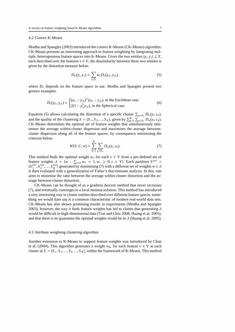
4.2 Convex K-Means
Modha and Spangler (2003) introduced the convex K-Means (CK-Means) algorithm.CK-Means presents an interesting approach to feature weighting by integrating mul-tiple, heterogeneous feature spaces into K-Means. Given the two entities{yi , y j} ⊆ Y,each described over the featuresv ∈ V, the dissimilarity between these two entities isgiven by the distortion measure below.
Dw(yi , y j) =∑
v∈V
wvDv(yiv, y jv), (5)
whereDv depends on the feature space in use. Modha and Spangler present twogeneric examples.
Dv(yiv, y jv) =
(yiv − y jv)T(yiv − y jv), in the Euclidean case
2(1− yTivy jv), in the Spherical case.
(6)
Equation (5) allows calculating the distortion of a specificcluster∑
yi∈SkDw(yi, ck),
and the quality of the clusteringS = {S1,S2, ...,SK}, given by∑K
k=1∑
yi∈SkDw(yi, ck).
CK-Means determines the optimal set of feature weights thatsimultaneously min-imises the average within-cluster dispersion and maximises the average between-cluster dispersion along all of the feature spaces, by consequence minimising thecriterion below.
W(S,C,w) =K∑
k=1
∑
yi∈Sk
Dw(yi , ck). (7)
This method finds the optimal weightwv for eachv ∈ V from a pre-defined set offeature weights∆ = {w :
∑
v∈V wv = 1,wv ≥ 0, v ∈ V}. Each partitionS(w)=
{S(w)1 ,S
(w)2 , ...,S
(w)K } generated by minimising (7) with a different set of weightsw ∈ ∆
is then evaluated with a generalization of Fisher’s discriminant analysis. In this, oneaims to minimise the ratio between the average within-cluster distortion and the av-erage between-cluster distortion.
CK-Means can be thought of as a gradient descent method that never increases(7), and eventually converges to a local minima solution. This method has introduceda very interesting way to cluster entities described over different feature spaces, some-thing we would dare say is a common characteristic of modern real-world data sets.CK-Means has also shown promising results in experiments (Modha and Spangler2003), however, the way it finds feature weights has led to claims that generating∆would be difficult in high-dimensional data (Tsai and Chiu 2008; Huang et al. 2005),and that there is no guarantee the optimal weights would be in∆ (Huang et al. 2005).
4.3 Attribute weighting clustering algorithm
Another extension to K-Means to support feature weights wasintroduced by Chanet al. (2004). This algorithm generates a weightwkv for each featurev ∈ V at eachcluster inS = {S1,S2, ...,Sk, ...,SK}, within the framework of K-Means. This method
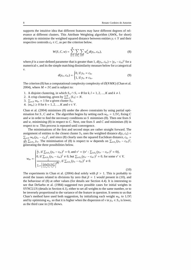
8 Renato Cordeiro de Amorim
supports the intuitive idea that different features may have different degrees of rel-evance at different clusters. This Attribute Weighting algorithm (AWK, for short)attempts to minimise the weighted squared distance betweenentitiesyi ∈ Y and theirrespective centroidsck ∈ C, as per the criterion below.
W(S,C,w) =K∑
k=1
∑
i∈Sk
∑
v∈V
wβkvd(yiv, ckv), (8)
whereβ is a user-defined parameter that is greater than 1,d(yiv, ckv) = |yiv − ckv|2 for a
numericalv, and its the simple matching dissimilarity measure below for a categoricalv.
d(yiv, ckv) =
0, if yiv = ckv
1, if yiv , ckv.(9)
The criterion (8) has a computational complexity complexity ofO(NMK) (Chan et al.2004), whereM = |V| and is subject to:
1. A disjoint clustering, in whichSk ∩ Sl = ∅ for k, l = 1, 2, ...,K andk , l.2. A crisp clustering, given by
∑Kk=1 |Sk| = N.
3.∑
v∈V wkv = 1 for a given clusterSk.4. {wkv} ≥ 0 for k = 1, 2, ...,K andv ∈ V.
Chan et al. (2004) minimises (8) under the above constraintsby using partial opti-misation forS, C andw. The algorithm begins by setting eachwkv = 1/|V|, fixing Candw in order to find the necessary conditions soS minimises (8). Then one fixesSandw, minimising (8) in respect toC. Next, one fixesS andC and minimises (8) inrespect tow. This process is repeated until convergence.
The minimisations of the first and second steps are rather straight forward. Theassignment of entities to the closest clusterSk uses the weighted distanced(yi, ck) =∑
v∈V wkv(yiv − ckv)2, and since (8) clearly uses the squared Euclidean distance,ckv =1|Sk|
∑
i∈Skyiv. The minimisation of (8) is respect tow depends on
∑
i∈Sk(yiv − ckv)2,
generating the three possibilities below.
wkv =
1v∗ , if
∑
i∈Sk(yiv − ckv)2
= 0, andv∗ = |{v′ :∑
i∈Sk(yiv′ − ckv′)2
= 0}|,
0, if∑
i∈Sk(yiv − ckv)2
, 0, but∑
i∈Sk(yiv′ − ckv′)2
= 0, for somev′ ∈ V,1
∑
j∈V
[∑
i∈Sk(yiv−ckv)2
∑
i∈Sk(yi j −ck j )
2
]1β−1
, if∑
i∈Sk(yiv − ckv)2
, 0.
(10)The experiments in Chan et al. (2004) deal solely withβ > 1. This is probably toavoid the issues related to divisions by zero thatβ = 1 would present in (10), andthe behaviour of (8) at other values (for details see Section4.4). It is interesting tosee that DeSarbo et al. (1984) suggested two possible cases for initial weights inSYNCLUS (details in Section 4.1), either to set all weights to the same number, or tobe inversely proportional to the variance of the feature in question. It seems to us thatChan’s method have used both suggestion, by initializing each weightwkv to 1/|V|and by optimisingwkv so that it is higher when the dispersion ofv in yiv ∈ Sk is lower,as the third case in (10) shows.

A survey on feature weighting based K-Means algorithms 9
There are some issues to have in mind when using this algorithm. The use of(9) may be problematic in certain cases as the range ofd(yiv, ckv) will be different de-pending on whetherv is numerical or categorical. Based on the work of Huang (1998)and Ng and Wong (2002), Chan et al. introduces a new parameterto balance the nu-merical and categorical parts of a mixed data set, in an attempt to avoid favouringeither part. In their paper they test AWK using different values for this parameter andthe best is determined as that resulting in the highest cluster recovery accuracy. Thisapproach is rather hard to follow in real-life clustering scenarios as no labelled datawould be present. This approach was only discussed in the experiments part of thepaper, not being present in the AWK description so it is ignored in our experiments.
Another point to note is that their experiments using real-life data sets, despite allexplanations about feature weights, use two weights for each feature. One of theserelates to the numerical features while the other relates tothose that are categorical.This approach was also not explained in the AWK original description and is ignoredin our experiments as well.
A final key issue to this algorithm, and in fact various others, is that there is noclear method to estimate the parameterβ. Instead, the authors state that their methodis not sensitive to a range of values ofβ, but unfortunately this is demonstrated withexperiments on synthetic data in solely two real-world datasets.
4.4 Weighted K-Means
Huang et al. (2005) introduced the Weighted K-Means (WK-Means) algorithm. WK-Means attempts to minimise the object function below, whichis similar to that ofChan et al. (2004), discussed in Section 4.3. However, unlike the latter, WK-Meansoriginally sets a single weightwv for each featurev ∈ V.
W(S,C,w) =K∑
k=1
∑
i∈Sk
∑
v∈V
wβvd(yiv, ckv), (11)
The Equation above is minimised using an iterative method, optimising (11) forS, C,andw, one at a time. During this process Huang et al. presents the two possibilitiesbelow for the update ofwv, with S andC fixed, subject toβ > 1.
wv =
0, if Dv = 01
∑hj=1
DvD j
1β−1
, if Dv , 0, (12)
where,
Dv =
K∑
k=1
∑
i∈Sk
d(yiv, ckv), (13)
andh is the number of features whereDv , 0. If β = 1, the minimisation of (11)follows thatwv′ = 1, andwv = 0, wherev′ , v, andDv′ ≤ Dv, for eachv ∈ V (Huanget al. 2005).

10 Renato Cordeiro de Amorim
The weightwβv in (11) makes the final clusteringS, and by consequence the cen-troids inC, dependant of the value ofβ. There are two possible critical values forβ, 0and 1. Ifβ = 0, Equation (11) becomes equivalent to that of K-Means (1). At β = 1,the weight of a single featurev ∈ V is set to one (that with the lowestDv), while allthe others are set to zero. Settingβ = 1 is probably not desirable in most problems.
The above critical values generate three intervals of interest. Whenβ < 0, wv
increases with an increase inDv. However, the negative exponent makeswβv smaller,so thatv has less of an impact on distance calculations. If 0< β < 1, wv increaseswith an increase inDv, so doeswβv. This goes against the principle that a feature witha small dispersion should have a higher weight, proposed by Chan et al. (2004) (per-haps inspired by SYNCLUS, see Section 4.1), and followed by Huang et al. (2005).If β > 1, wv decreases with an increase inDv, and so doeswβv, very much the desiredeffect of decreasing the impact of a featurev in (11) whoseDv is high.
WK-Means was later extended to support fuzzy clustering (Liand Yu 2006),as well as cluster dependant weights (Huang et al. 2008). Thelatter allows WK-Means to support weights with different degrees of relevance at different clusters,each represented bywkv. This required a change in the criterion to be minimisedto W(S,C,w) =
∑Kk=1∑
i∈Sk
∑
v∈V wβkvd(yiv, ckv), and similar changes to other relatedequations.
In this new version, the dispersion of a variablev ∈ V at a clusterSk is given byDkv =
∑
i∈Sk(d(yiv, ckv) + c), wherec is a user-defined constant. The authors suggest
that in practicec can be chosen as the average dispersion of all features in thedata set.More importantly, the adding ofc addresses a considerable shortcoming. A featurewhose dispersionDkv in a particular clusterSk is zero should not be assigned a weightof zero when in factDkv = 0 indicates thatv may be an important feature to identifyclusterSk. An obvious exception is if
∑Kk=1 Dkv = 0 for a givenv, however, such
feature should normally be removed in the data pre-processing stage.
Although there have been improvements, the final clusteringis still highly depen-dant on the exponent exponentβ. It seems to us that the selection ofβ depends on theproblem at hand, but unfortunately there is no clear strategy for its selection. We alsofind that the lack of relationship betweenβ and the distance exponent (two in the caseof the Euclidean squared distance) avoids the possibility of seen the final weights asfeature re-scaling factors. Finally, although WK-Means supports cluster-dependantfeatures, all features are treated as if they were a homogeneous feature space, verymuch unlike CK-Means (details in Section 4.2).
4.5 Entropy Weighting K-Means
The Entropy Weighting K-Means algorithm (EW-KM) (Jing, Ng,and Huang 2007)minimises the within cluster dispersion while maximising the negative entropy. Thereasoning behind this is to stimulate more dimensions to contribute to the identifica-tion of clusters in high-dimensional sparse data, avoidingproblems related to identi-fying such clusters using only a few dimensions.

A survey on feature weighting based K-Means algorithms 11
With the above in mind, Jing, Ng, and Huang (2007) devised thefollowing crite-rion for EW-KM:
W(S,C,w) =K∑
k=1
N∑
i∈Sk
∑
v∈V
wkv(yiv − ckv)2+ γ∑
v∈V
wkvlogwkv
, (14)
subject to∑
v∈V wkv = 1, {wkv} ≥ 0, and a crisp clustering. In the criterion above,one can easily identify that the first term is the weighted sumof the within clusterdispersion. The second term, in whichγ is a parameter controlling the incentive forclustering in more dimensions, is the negative weight entropy.
The calculation of weights in EW-KM occurs as an extra step inrelation to K-Means, but still with a time complexity ofO(rNMK) wherer is the number of itera-tions the algorithm takes to converge. Given a clusterSk, the weight of each featurev ∈ V is calculated one at a time with the equation below.
wkv =exp(−Dkv
γ)
∑
j∈V exp(−Dk j
γ), (15)
whereDkv represents the dispersion of featurev in the clusterSk, given byDkv =∑
i∈Sk(yiv − ckv)2. As one would expect, the minimisation of (14) uses partial optimi-
sation forw, C, andS. First,C andw are fixed and (14) is minimised in respect toS. Next,S andw are fixed and (14) is minimised in respect toC. In the final step,S andC are fixed, and (14) is minimised in respect tow. This adds a single step toK-Means, used to calculate feature weights.
The R packageweightedKmeansfound at CRAN includes an implementation ofthis algorithm, which we decided to use in our experiments (details in Sections 5and 6). Jing, Ng, and Huang (2007) presents extensive experiments, with syntheticand real-world data. These experiments show EW-KM outperforming various otherclustering algorithms. However, there are a few points we should note. First, it issomewhat unclear how a user should choose a precise value forγ. Also, most ofthe algorithms used in the comparison required a parameter as well. Although weunderstand it would be too laborious to analyse a large rangeof parameters for eachof these algorithms, there is no much indication on reasoning behind the choicesmade.
4.6 Improved K-Prototypes
Ji et al. (2013) have introduced the Improved K-Prototypes clustering algorithm (IK-P), which minimises the WK-Means criterion (11), with influences from k-prototype(Huang 1998). IK-P introduces the concept of distributed centroid to clustering, al-lowing the handling of categorical features by adjusting the distance calculation totake into account the frequency of each category.
IK-P treats numerical and categorical features differently, but it is still able torepresent the clusterSk of a data setY containing mixed type, data with a single cen-troidck = {ck1, ck2, ..., ck|V|}. Given a numerical featurev, ckv =
1|Sk|
∑
i∈Skyiv, the center

12 Renato Cordeiro de Amorim
given by the Euclidean distance. A categorical featurev containingL categoriesa ∈ v,hasckv = {{a1
v, ω1kv}, {a
2v, ω
2kv}, ..., {a
lv, ω
lkv}, ..., {a
Lv , ω
Lkv}}. This representation for a cat-
egoricalv allows each categorya ∈ v to have a weightωlkv =
∑
i∈Skη(yiv), directly
related to its frequency in the data setY.
η(yiv) =
1∑
i∈Sk1, if yiv = al
v,
0, if yiv , alv.
(16)
Such modification also requires a re-visit of the distance function in (11). The dis-tance is re-defined to the below.
d(yiv, ckv) =
|yiv − ckv|, if v is numerical,
ϕ(yiv − ckv), if v is categorical,(17)
whereϕ(yiv − ckv) =∑K
k=1 ϑ(yiv, alv),
ϑ(yiv, akv) =
0, if yiv = alv,
ωkiv, if yiv , al
v,(18)
IK-P presents some very interesting results (Ji et al. 2013), outperforming otherpopular clustering algorithms such as k-prototype, SBAC, and KL-FCM-GM (Chatzis2011; Ji et al. 2012). However, the algorithm still leaves some open questions.
For instance, Ji et al. (2013) present experiments on six data sets (two of whichbeing different versions of the same data set) settingβ = 8, but it is not clear whetherthe good results provided by this particularβ would generalize to other data sets.Given a numerical feature, IK-P applies the Manhattan distance (17), however, cen-troids are calculated using the mean. The center of the Manhattan distance is given bythe median rather than the mean, this is probably the reason why Ji et al. found it nec-essary to allow the user to set a maximum numbers of iterations to their algorithm.Now, even if the algorithm converges, most likely it would converge in a smallernumber of iterations if the distance used for the assignments of entities was alignedto that used for obtaining the centroids. Finally, whiled(yiv, ckv) for a categoricalvhas a range in the interval [0, 1], the same is not true ifv is numerical, however, Jiet al. (2013) make no mention to data standardization.
4.7 Intelligent Minkowski Weighted K-Means
Previously, we have extended WK-Means (details in Section 4.4) by introducing theintelligent Minkowski Weighted K-Means (iMWK-Means) (De Amorim and Mirkin2012). In its design, we aimed to propose a deterministic algorithm supporting non-elliptical clusters with weights that could be seen as feature weighting factors. To doso, we combined the Minkowski distance and intelligent K-Means (Mirkin 2012), amethod that identifies anomalous patterns in order find the number of clusters in adata set, as well as good initial centroids.

A survey on feature weighting based K-Means algorithms 13
Below, we show the Minkowski distance between the entitiesyi andy j , describedover featuresv ∈ V.
d(yi, y j) = (∑
v∈V
|yiv − y jv|p)1/p, (19)
wherep is a user-defined parameter. Ifp equals 1, 2, or∞, Equation (19) is equivalentto the the Manhattan, Euclidean and Chebyshev distances, respectively. Assuminga given data set has two dimensions (for easy visualisation), the distance bias ofa clustering algorithm using (19) would be towards clusterswhose shape are anyinterpolation between a diamond (p = 1) and a square (p = ∞), clearly going througha circle (p = 2). This is considerably more flexible than algorithms basedsolely onthe squared Euclidean distance, as these recover clusters biased towards circles only.One can also see the Minkowski distance as a multiple of the power mean of thefeature-wise differences betweenyi andy j .
The iMWK-Means algorithm calculates distances using (20),a weighted versionof thepth root of (19). The use of a root is analogous to the frequent useof the squaredEuclidean distance in K-Means.
d(yi , y j) =∑
v∈V
wpkv|yiv − y jv|
p, (20)
where the user-defined parameterp scales the distance as well as well as the clusterdependent weightwkv. This way the feature weights can be seen as feature re-scalingfactors, this is not possible for WK-Means whenβ , 2. Re-scaling a data set withthese feature re-scaling factors increases the likelihoodof various cluster validityindices to lead to the correct number of clusters (De Amorim and Hennig 2015).With (20) one can reach the iMWK-Means criterion below.
W(S,C,w) =K∑
k=1
∑
i∈Sk
∑
v∈V
wpkv|yiv − ckv|
p. (21)
The update ofwkv, for eachv ∈ V andk = 1, 2, ...,K, follows the equation below.
wkv =1
∑
u∈VDkvp
Dkup
1p−1
, (22)
where the dispersion of featurev in clusterk is now dependant on the exponentp,Dkvp =
∑
i∈Sk|yiv − ckv|
p+ c, andc is a constant equivalent to the average dispersion.
The update of the centroid of clusterSk on featurev, ckv also depends on the valueof p. At values ofp 1, 2, and∞, the center of (19) is given by the median, mean andmidrange, respectively. Ifp < {1, 2,∞} then the center can be found using a steepestdescend algorithm (De Amorim and Mirkin 2012).
The iMWK-Means algorithm deals with categorical features by transformingthem in numerical, following a method described by Mirkin (2012). In this method,a given categorical featurev with L categories is replaced byL binary features, eachrepresenting one of the original categories. For a given entity yi , only the binaryfeature representingyiv is set to one, all others are set to zero. The concept of dis-tributed centroid (Ji et al. 2013) can also be applied to our algorithm (De Amorim and
14 Renato Cordeiro de Amorim
Makarenkov to appear), however, in order to show a single version of our method wedecided not to follow the latter here.
Clearly, the chosen value ofp has a considerable impact on the final clusteringgiven by iMWK-Means. De Amorim and Mirkin (2012) introduceda semi-supervisedalgorithm to estimate a goodp, requiring labels for 20% of the entities inY. Later,the authors showed that it is indeed possible to estimate a good value forp using only5% of labelled data under the same semi-supervised method, and presented a newunsupervised method to estimatep, requiring no labelled samples (De Amorim andMirkin 2014).
The iMWK-Means proved to be superior to various other algorithms, includingWK-Means with cluster dependant weights (De Amorim and Mirkin 2012). How-ever, iMWK-Means also has room for improvement. Calculating a centroid for ap < {1, 2,∞} requires the use of a steepest descent method. This can be time consum-ing, particularly when compared with other algorithms defining ckv =
1|Sk|
∑
i∈Skyiv.
Although iMWK-Means allows for a distance bias towards non-elliptical clusters, bysettingp , 2, it assumes that all clusters should be biased towards the same shape.
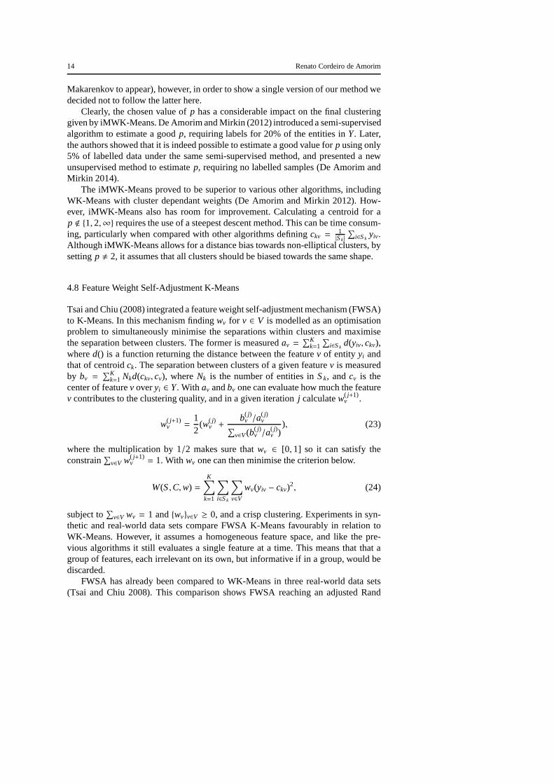
4.8 Feature Weight Self-Adjustment K-Means
Tsai and Chiu (2008) integrated a feature weight self-adjustment mechanism (FWSA)to K-Means. In this mechanism findingwv for v ∈ V is modelled as an optimisationproblem to simultaneously minimise the separations withinclusters and maximisethe separation between clusters. The former is measuredav =
∑Kk=1∑
i∈Skd(yiv, ckv),
whered() is a function returning the distance between the featurev of entity yi andthat of centroidck. The separation between clusters of a given featurev is measuredby bv =
∑Kk=1 Nkd(ckv, cv), whereNk is the number of entities inSk, andcv is the
center of featurev overyi ∈ Y. With av andbv one can evaluate how much the featurev contributes to the clustering quality, and in a given iteration j calculatew( j+1)
v .
w( j+1)v =
12
(w( j)v +
b( j)v /a
( j)v
∑
v∈V(b( j)v /a
( j)v )
), (23)
where the multiplication by 1/2 makes sure thatwv ∈ [0, 1] so it can satisfy theconstrain
∑
v∈V w( j+1)v = 1. With wv one can then minimise the criterion below.
W(S,C,w) =K∑
k=1
∑
i∈Sk
∑
v∈V
wv(yiv − ckv)2, (24)
subject to∑
v∈V wv = 1 and{wv}v∈V ≥ 0, and a crisp clustering. Experiments in syn-thetic and real-world data sets compare FWSA K-Means favourably in relation toWK-Means. However, it assumes a homogeneous feature space,and like the pre-vious algorithms it still evaluates a single feature at a time. This means that that agroup of features, each irrelevant on its own, but informative if in a group, would bediscarded.
FWSA has already been compared to WK-Means in three real-world data sets(Tsai and Chiu 2008). This comparison shows FWSA reaching anadjusted Rand

A survey on feature weighting based K-Means algorithms 15
index (ARI) 0.77 when applied to the Iris data set, while WK-Means reached only0.75. The latter ARI was obtained by settingβ = 6, but our experiments (details inSection 6) show that WK-Means may reach 0.81. The differencemay be related tohow the data was standardised, as well as howβ was set as here we found the best ateach run. Of course, the fact that FWSA does not require a user-defined parameter isa considerable advantage.
4.9 FG-K-Means
The FG-K-Means (FGK) algorithm (Chen et al. 2012) extends K-Means by applyingweights at two levels, features and clusters of features. This algorithm has been de-signed to deal with large data sets whose data comes from multiple sources. Each oftheT data sources provides a subset of featuresG = {G1,G2, ...,GT}, whereGt , ∅,Gt ⊂ V, Gt ∩ Gs = ∅ for t , s and 1≤ t, s ≤ T, and∪Gt = V. Given a clusterSk,FGK identifies the degree of relevance of a featurev, represented bywkv, as well asthe relevance of a group of featuresGt, represented byωkt. Unlike SYNCLUS (de-tails in Section 4.1), FGK does not require the weights of thegroups of features to beentered by the user. FGK updates the K-Means criterion (1) toinclude bothwkv andωkt, as we show below.
W(S,C,w, ω) =K∑
k=1
∑
i∈Sk
T∑
t=1
∑
v∈Gt
ωktwkvd(yiv, ckv) + λT∑
t=1
ωktlog(ωkt) + η∑
v∈V
wkvlog(wkv)
,
(25)whereλ andη are user-defined parameters, adjusting the distributions of the weightsrelated to the groups of features inG, and each of the featuresv ∈ V, respectively.The minimisation of (25) is subject to a crisp clustering in which any given entityyi ∈ Y is assigned to a single clusterSk. The feature group weights are subject to∑K
k=1ωkt = 1, 0 < ωkt < 1, for 1 ≤ t ≤ T. The feature weights are subject to∑
v∈Gtwkv = 1, 0< wkv < 1, for 1≤ k ≤ K and 1≤ t ≤ T.
Given a numericalv, the functiond in (25) returns the squared Euclidean distancebetweenyiv andckv, given by (yiv − ckv)2. A categoricalv leads tod returning one ifyiv = ckv, and zero otherwise, very much like (9). The update of each feature weightfollows the equation below.
wkv =exp(−Ekv
η)
∑
h∈Gtexp(−Ekh
η), (26)
whereEkv =∑
i∈Skωktd(yiv, ckv), and t is the index of the feature group to which
featurev is assigned to. The update of the feature group weights follows.
ωkt =exp(−Dkt
λ)
∑Ts=1 exp(−Dks
λ), (27)
where,Dkt =∑
i∈Sk
∑
v∈Gtwkvd(yiv, ckv). Clusterings generated by FGK are heavily
dependant onλ andη. These parameters must set to positive real values. Large val-ues forλ andη lead to weights to be more evenly distributed, so more subspaces

16 Renato Cordeiro de Amorim
contribute to the clustering. Low values lead to weights being more concentrated onfewer subspaces, each of these having a larger contributionto the clustering.
FGK has a time complexity ofO(rNMK), wherer is the number of iterations thisalgorithm takes to complete (Chen et al. 2012). It has outperformed K-Means, WK-Means (see Section 4.4), LAC (Domeniconi et al. 2007) and EW-KM (see Section4.5), but it also introduces new open questions. This particular method was designedaiming to deal with high-dimensional data, however, it is not clear howλ andη shouldbe estimated. This issue makes it rather hard to use FGK in real-world problems. Wefind that it would also be interesting to see a generalizationof this method to use otherdistance measures, allowing a different distance bias.
5 Setting of the experiments
In our experiments we have used real-world as well as synthetic data sets. The formerwere obtained from the popular UCI machine learning repository (Lichman 2013)and include data sets with different combinations of numerical and categorical fea-tures, as we show in Table 1.
Table 1 Real-world data sets used in our comparison experiments.
Entities Clusters Original featuresNumerical Categorical Total
Australian credit 690 2 6 8 14Balance scale 625 2 0 4 4Breast cancer 699 2 9 0 9Car evaluation 1728 4 0 6 6Ecoli 336 8 7 0 7Glass 214 6 9 0 9Heart (Statlog) 270 2 6 7 13Ionosphere 351 2 33 0 33Iris 150 3 4 0 4Soybean 47 4 0 35 35Teaching Assistant 151 3 1 4 5Tic Tac Toe 958 2 0 9 9Wine 178 3 13 0 13
The synthetic data sets contain spherical Gaussian clusters so that the covariancematrices are diagonal with the same diagonal valueσ2 generated at each cluster ran-domly between 0.5 and 1.5. All centroid components were generated independentlyfrom a Gaussian distribution with zero mean and unity variance. The cardinality ofeach cluster was generated following an uniformly random distribution, constrainedto a minimum of 20 entities. We have generated 20 data sets under each of the fol-lowing configurations: (i) 500x4-2, 500 entities over four features partitioned intotwo clusters; (ii) 500x10-3, 500 entities over 10 features partitioned into three clus-ters; (iii) 500x20-4, 500 entities over 20 features partitioned into four clusters; (iv)500x50-5, 500 entities over 50 features partitioned into five clusters.

A survey on feature weighting based K-Means algorithms 17
Unfortunately, we do not know the degree of relevance of eachfeature in all ofour data sets. For this reason we decided that our experiments should also includedata sets to which we have added noise features. Given a data set, for each of its cat-egorical features we have added a new feature composed entirely of uniform randomintegers (each integer simulates a category). For each of its numerical features wehave added a new feature composed entirely of uniform randomvalues. In both casesthe new noise feature has the same domain as the original feature. This approach haseffectively doubled the number of features in each data set,as well as the number ofdata sets used in our experiments.
Prior to our experiments we have standardised the numericalfeatures of each ofour data sets as per the equation below.
yiv =yiv − yv
range(yv), (28)
whereyv =1N
∑Ni=1 yiv, andrange(yv) = max({yiv}
Ni=1) − min({yiv}
Ni=1). Our choice of
using (28) instead of the popularz-score is perhaps easier to explain with an example.Lets imagine two features, unimodalv1 and multimodalv2. The standard deviation ofv2 would be higher than that ofv1 which means that thez-score ofv2 would be lower.Thus, the contribution ofv2 to the clustering would be lower than that ofv1 even so itis v2 that has a cluster structure. Arguably, a disadvantage of using (28) is that it canbe detrimental to algorithms based on other standardisation methods (Steinley andBrusco 2008b), not included in this paper.
We have standardised the categorical features for all but those experiments withthe Attribute weighting and Improved K-Prototypes algorithms (described in Sec-tions 4.3 and 4.6, respectively). These two algorithms define distances for categoricalfeatures, so transforming the latter to numerical is not required. Given a categoricalfeaturev containingq categories we substitutev by q new binary features. In a givenentity yi only a single of these new features is set to one, that representing the cate-gory originally inyiv. We then numerically standardise each of the new features bysubtracting it by its mean. The mean of a binary feature is in fact its frequency, so abinary feature representing a category with a high frequency contributes less to theclustering than one with a low frequency. In terms of data pre-processing, we alsomade sure that all features in each data set had a range higherthan zero. Featureswith a range of zero are not meaningful so they were removed.
Unfortunately, we found it very difficult to set a fair comparison including allalgorithms we describe in this paper. SYNCLUS and FG-K-Means(described in Sec-tions 4.1 and 4.9, respectively) go a step further in featureweighting by allowingweights for feature groups. However, they both require the user to meaningfully groupfeaturesv ∈ V into T partitionsG = {G1,G2, ...,GT} with SYNCLUS also requestingthe user to set a weight for each of these groups. Even if we hadenough informationto generateG it would be unfair to provide this extra information to some algorithmsand not to others. If we were to group features randomly we would be providing thesetwo algorithms with misleading information more often thannot, which would surelyhave an impact on their cluster recovery ability. If we were to set a single group offeatures and give this group a weight of one then we would be removing the mainadvantage of using these algorithms, and in fact FG-K-Meanswould be equivalent to

18 Renato Cordeiro de Amorim
EW-KM. Convex K-Means (Section 4.2) also goes a step furtherin feature weighting,it does so by integrates multiple, heterogeneous feature spaces. Modha and Spangler(2003) demonstrates that with the Euclidean and Spherical cases. However, there islittle information regarding the automatic detection of the appropriate space given afeaturev ∈ V, a very difficult problem indeed. For these reasons we decided not toinclude these three algorithms in our experiments.
6 Results and discussion
In our experiments we do have a set of labels for each data set.This allows us tomeasure the cluster recovery of each algorithm in terms of the adjusted Rand index(ARI) (Hubert and Arabie 1985) between the generated clustering and the knownlabels.
ARI =
∑
i j
(
ni j
2
)
− [∑
i
(
ai2
)
∑
j
(
bj
2
)
]/(
n2
)
12[∑
i
(
ai2
)
+
∑
j
(
bj
2
)
] − [∑
i
(
ai2
)
∑
j
(
bj
2
)
]/(
n2
) , (29)
whereni j = |Si ∩ S j |, ai =∑K
j=1 |Si ∩ S j | andbi =∑K
i=1 |Si ∩ S j |.FWSA is the only algorithm we experiment with that does not require an extra pa-
rameter from the user. This is clearly an important advantage as estimating optimumparameters is not a trivial problem, and in many cases the authors of the algorithmsdo not present a clear estimation method.
The experiments we show here do not deal with parameter estimation. Instead,we determine the optimum parameter for a given algorithm by experimenting withvalues from 1.0 to 5.0 in steps of 0.1. The only exception are the experiments withEW-KM where we apply values from 0 to 5.0 in steps of 0.1, this is because EW-KMis the only algorithm in which a parameter between zero and one is also appropriate.Most of the algorithms we experiment with are non-deterministic (iMWK-Means isthe only exception), so we run each algorithm at each parameter 100 times and selectas the optimum parameter that with the highest average ARI.
Tables 2 and 3 show the results of our experiments on the real-world data setswithout noise features added to them (see Table 1). We show the average (togetherwith the standard deviation) and maximum ARI for what we found to be the optimumparameter for each data set we experiment with. There are different comparisons wecan make, particularly when one of the algorithms is deterministic, iMWK-Means. Ifwe compare the algorithms in terms of their expected ARI, given a good parameter,then we can see that in 9 data sets iMWK-Means reaches the highest ARI. We runeach non-deterministic algorithm 100 times for each parameter value. If we take intoaccount solely the highest ARI over these 100 runs then the EW-KM reaches thehighest ARI overall in 9 data sets, while IK-P does so in six. Still looking only atthe highest ARI, the FWSA algorithm (the only algorithm not to require an extraparameter) reaches the highest ARI in four data sets, the same number as AWK andWK-Means. Another point of interest is that the best parameter we could find foriMWK-Means was the same in four data sets.
Tables 4 and 5 show the results of our experiments on the real-world data setswith noise features added to them. Given a data setY, for eachv ∈ V we add a new

A survey on feature weighting based K-Means algorithms 19
Table 2 Experiments with the real-world data sets with no added noise features. The standard deviationcan be found after the backslash under the mean. Par refers tothe parameter value required by the algo-rithm.
Attribute Weighting Weighted K-Means Entropy WKARI ARI ARI
Mean Max Par Mean Max Par Mean Max ParAustralian 0.15/0.11 0.50 4.9 0.19/0.23 0.50 2.2 0.31/0.190.50 0.90Balance 0.03/0.03 0.19 3.4 0.04/0.04 0.18 4.7 0.04/0.05 0.23 2.10Breast c. 0.68/0.20 0.82 4.5 0.83/0.00 0.83 2.6 0.85/0.01 0.87 1.10Car eva. 0.07/0.05 0.22 2.6 0.04/0.05 0.13 1.2 0.07/0.06 0.22 4.60Ecoli 0.02/0.02 0.04 2.5 0.42/0.06 0.57 3.5 0.45/0.09 0.72 0.10Glass 0.15/0.03 0.22 3.7 0.19/0.04 0.28 2.8 0.17/0.03 0.28 0.10Heart 0.21/0.16 0.45 4.7 0.18/0.07 0.27 1.1 0.33/0.10 0.39 3.10Ionosphere 0.14/0.08 0.25 1.2 0.18/0.05 0.34 1.2 0.18/0.000.21 0.70Iris 0.80/0.16 0.89 1.6 0.81/0.11 0.89 3.9 0.71/0.14 0.82 0.30Soybean 0.57/0.18 1.00 3.5 0.78/0.22 1.00 3.1 0.74/0.20 1.00 0.10Teaching A. 0.02/0.01 0.05 1.9 0.02/0.01 0.07 4.0 0.03/0.020.10 0.20Tic Tac Toe 0.02/0.03 0.07 1.4 0.03/0.04 0.15 4.1 0.02/0.03 0.15 1.00Wine 0.76/0.06 0.82 4.8 0.85/0.02 0.90 4.4 0.82/0.05 0.90 0.30
Table 3 Experiments with the real-world data sets with no added noise features. The standard deviationcan be found after the backslash under the mean. Par refers tothe parameter value required by the al-gorithm. IMWK-Means is a deterministic algorithm and FWSA does not require a parameter, hence thedashes.
Improved K-P Intelligent Minkowski WK Feature Weight Self Adj.ARI ARI ARI
Mean Max Par Mean Max Par Mean Max ParAustralian 0.15/0.08 0.20 4.7 - 0.50 1.1 0.20/0.21 0.50 -Balance 0.04/0.05 0.23 1.3 - 0.09 3.3 0.03/0.03 0.15 -Breast c. 0.74/0.00 0.74 4.9 - 0.85 4.6 0.81/0.12 0.83 -Car eva. 0.03/0.05 0.22 5.0 - 0.13 2.0 0.04/0.06 0.22 -Ecoli 0.46/0.00 0.46 3.0 - 0.04 2.5 0.37/0.06 0.52 -Glass 0.21/0.06 0.31 4.4 - 0.28 4.6 0.16/0.04 0.25 -Heart 0.31/0.08 0.36 4.6 - 0.31 2.9 0.15/0.10 0.31 -Ionosphere 0.14/0.07 0.43 1.9 - 0.21 1.1 0.17/0.03 0.21 -Iris 0.78/0.21 0.90 1.2 - 0.90 1.1 0.77/0.19 0.89 -Soybean 0.87/0.16 0.95 2.4 - 1.00 1.8 0.71/0.23 1.00 -Teaching A. 0.01/0.01 0.04 4.0 - 0.04 2.2 0.02/0.01 0.05 -Tic Tac Toe 0.02/0.03 0.15 2.8 - 0.02 1.1 0.02/0.02 0.15 -Wine 0.86/0.01 0.86 4.3 - 0.82 1.6 0.70/0.13 0.82 -
feature toY composed entirely of uniform random values (integers in thecase ofa categoricalv) with the same domain asv. This effectively doubles the cardinalityof V. In this set of experiments the Improved K-Prototype was unable to find eightclusters in the Ecoli data set. We believe this issue is related to the data spread. Thethird feature of this particular data set has only 10 entities with a value other than0.48. The fourth feature has a single entity with a value other than 0.5. Clearly onthe top of these two issues we have an extra seven noise features. Surely one couldargue that features three and four could be removed from the data set as they areunlikely to be informative. However, we decided not to startopening concessions to
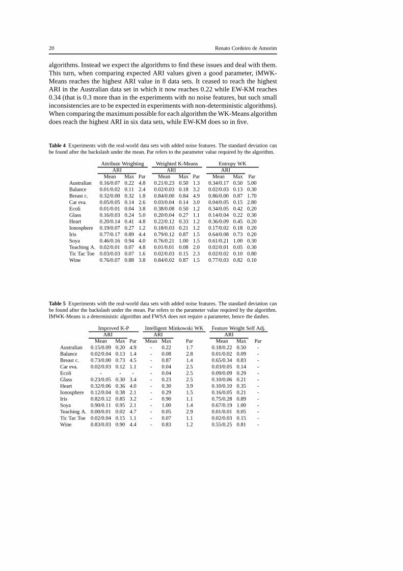
20 Renato Cordeiro de Amorim
algorithms. Instead we expect the algorithms to find these issues and deal with them.This turn, when comparing expected ARI values given a good parameter, iMWK-Means reaches the highest ARI value in 8 data sets. It ceased to reach the highestARI in the Australian data set in which it now reaches 0.22 while EW-KM reaches0.34 (that is 0.3 more than in the experiments with no noise features, but such smallinconsistencies are to be expected in experiments with non-deterministic algorithms).When comparing the maximum possible for each algorithm the WK-Means algorithmdoes reach the highest ARI in six data sets, while EW-KM does so in five.
Table 4 Experiments with the real-world data sets with added noise features. The standard deviation canbe found after the backslash under the mean. Par refers to theparameter value required by the algorithm.
Attribute Weighting Weighted K-Means Entropy WKARI ARI ARI
Mean Max Par Mean Max Par Mean Max ParAustralian 0.16/0.07 0.22 4.8 0.21/0.23 0.50 1.3 0.34/0.170.50 5.00Balance 0.01/0.02 0.11 2.4 0.02/0.03 0.18 3.2 0.02/0.03 0.13 0.30Breast c. 0.32/0.00 0.32 1.8 0.84/0.00 0.84 4.9 0.86/0.00 0.87 1.70Car eva. 0.05/0.05 0.14 2.6 0.03/0.04 0.14 3.0 0.04/0.05 0.15 2.80Ecoli 0.01/0.01 0.04 3.8 0.38/0.08 0.50 1.2 0.34/0.05 0.42 0.20Glass 0.16/0.03 0.24 5.0 0.20/0.04 0.27 1.1 0.14/0.04 0.22 0.30Heart 0.20/0.14 0.41 4.8 0.22/0.12 0.33 1.2 0.36/0.09 0.45 0.20Ionosphere 0.19/0.07 0.27 1.2 0.18/0.03 0.21 1.2 0.17/0.020.18 0.20Iris 0.77/0.17 0.89 4.4 0.79/0.12 0.87 1.5 0.64/0.08 0.73 0.20Soya 0.46/0.16 0.94 4.0 0.76/0.21 1.00 1.5 0.61/0.21 1.00 0.30Teaching A. 0.02/0.01 0.07 4.8 0.01/0.01 0.08 2.0 0.02/0.010.05 0.30Tic Tac Toe 0.03/0.03 0.07 1.6 0.02/0.03 0.15 2.3 0.02/0.02 0.10 0.80Wine 0.76/0.07 0.88 3.8 0.84/0.02 0.87 1.5 0.77/0.03 0.82 0.10
Table 5 Experiments with the real-world data sets with added noise features. The standard deviation canbe found after the backslash under the mean. Par refers to theparameter value required by the algorithm.IMWK-Means is a deterministic algorithm and FWSA does not require a parameter, hence the dashes.
Improved K-P Intelligent Minkowski WK Feature Weight Self Adj.ARI ARI ARI
Mean Max Par Mean Max Par Mean Max ParAustralian 0.15/0.09 0.20 4.9 - 0.22 1.7 0.18/0.22 0.50 -Balance 0.02/0.04 0.13 1.4 - 0.08 2.8 0.01/0.02 0.09 -Breast c. 0.73/0.00 0.73 4.5 - 0.87 1.4 0.65/0.34 0.83 -Car eva. 0.02/0.03 0.12 1.1 - 0.04 2.5 0.03/0.05 0.14 -Ecoli - - - - 0.04 2.5 0.09/0.09 0.29 -Glass 0.23/0.05 0.30 3.4 - 0.23 2.5 0.10/0.06 0.21 -Heart 0.32/0.06 0.36 4.0 - 0.30 3.9 0.10/0.10 0.35 -Ionosphere 0.12/0.04 0.38 2.1 - 0.29 1.5 0.16/0.05 0.21 -Iris 0.82/0.12 0.85 3.2 - 0.90 1.1 0.75/0.28 0.89 -Soya 0.90/0.11 0.95 2.1 - 1.00 1.4 0.67/0.19 1.00 -Teaching A. 0.00/0.01 0.02 4.7 - 0.05 2.9 0.01/0.01 0.05 -Tic Tac Toe 0.02/0.04 0.15 1.1 - 0.07 1.1 0.02/0.03 0.15 -Wine 0.83/0.03 0.90 4.4 - 0.83 1.2 0.55/0.25 0.81 -

A survey on feature weighting based K-Means algorithms 21
Tables 6 and 7 show the results of our experiments on the synthetic data setswith and without noise features. Given a data setY, for eachv ∈ V we have addeda new feature toY containing uniformly random noise in the same domain as thatofv, very much like what we did in the real-world data sets. The only difference is thatin the synthetic data sets we do not have categorical features and we know that theycontain Gaussian clusters (see Section 5). We have 20 data sets for each of the data setconfigurations, hence, the values under max represent the average of the maximumARI obtained in each of the 20 data sets, as well as the standard deviation of thesevalues.
In this set of experiments iMWK-Means reached the highest expected ARI in alldata sets, with and without noise features. If we compare solely the maximum possi-ble ARI per algorithm WK-Means reaches the highest ARI in three data set config-urations with no noise features added to them, and in two of the data sets with noisefeatures. AWK also reaches the highest ARI in two of the configurations Clearly,
Table 6 Experiments with the synthetic data sets, with and without noise features. The standard devia-tion can be found after the backslash under the mean. Par refers to the parameter value required by thealgorithm.
Attribute Weighting Weighted K-Means Entropy WKARI ARI ARI
Mean Max Par Mean Max Par Mean Max ParNo noise500x4-2 0.50/0.36 0.61/0.31 4.11/1.21 0.61/0.32 0.62/0.31 3.28/1.26 0.62/0.30 0.66/0.26 2.35/1.15500x10-3 0.62/0.20 0.83/0.11 4.55/0.53 0.68/0.20 0.85/0.10 3.10/1.05 0.67/0.20 0.84/0.10 0.83/0.39500x20-4 0.74/0.22 0.98/0.02 4.09/0.66 0.75/0.25 0.99/0.02 3.11/1.02 0.75/0.24 0.98/0.03 0.35/0.22500x50-5 0.83/0.18 1.00/0.01 3.48/1.03 0.82/0.19 1.00/0.00 3.62/0.99 0.80/0.19 1.00/0.00 0.24/0.12With noise500x4-2 0.29/0.38 0.60/0.32 2.93/1.11 0.27/0.37 0.61/0.32 1.46/0.80 0.34/0.33 0.56/0.29 0.29/0.16500x10-3 0.59/0.20 0.80/0.13 4.19/0.78 0.61/0.23 0.85/0.10 1.29/0.15 0.54/0.25 0.78/0.14 0.32/0.26500x20-4 0.73/0.22 0.98/0.03 3.78/0.90 0.71/0.25 0.93/0.19 1.37/0.26 0.81/0.14 0.95/0.06 0.34/0.10500x50-5 0.83/0.18 1.00/0.01 3.14/0.81 0.82/0.20 0.98/0.10 2.01/1.22 0.84/0.15 1.00/0.01 0.52/0.41
there are other comparisons we can make using all algorithmsdescribed in Section4. Based on the information we present in Section 4 about eachalgorithm, as wellas the cluster recovery results we present in this section, we have defined eight char-acteristics we believe are desirable for any K-Means based clustering algorithm thatimplements feature weighting. Table 8 shows our comparison, which we now de-scribe one characteristic at a time.
No extra user-defined parameter. Quite a few of the algorithms we describe inSection 4 require an extra parameter to be defined by the user.By tuning this pa-rameter (or these parameters, in the case of FGK) each of these algorithms is able toachieve high accuracy in terms of cluster recovery. However, it seems to us that thisparameter estimation is a non-trivial task, particularly because the optimum value isproblem dependant. This makes it very difficult to suggest a generally good parame-ter value (of course this may not be the case if one knows how the data is distributed).Since different values for a parameter tend to result in different clusterings, one couldattempt to estimate the best clustering by applying a clustering validation index (Ar-belaitz et al. 2013; De Amorim and Mirkin 2014), consensus clustering (Goder and

22 Renato Cordeiro de Amorim
Table 7 Experiments with the synthetic data sets, with and without noise features. The standard devia-tion can be found after the backslash under the mean. Par refers to the parameter value required by thealgorithm. IMWK-Means is a deterministic algorithm and FWSA does not require a parameter, hence thedashes.
Improved K-P Intelligent Minkowski WK Feature Weight Self Adj.ARI ARI ARI
Mean Max Par Mean Max Par Mean Max ParNo noise500x4-2 0.45/0.37 0.59/0.32 3.69/1.18 - 0.63/0.30 3.18/1.31 0.38/0.36 0.57/0.33 -500x10-3 0.60/0.21 0.81/0.12 3.85/0.85 - 0.71/0.18 2.51/0.83 0.42/0.23 0.67/0.24 -500x20-4 0.74/0.25 0.98/0.04 3.74/1.03 - 0.90/0.17 2.58/1.05 0.64/0.24 0.94/0.15 -500x50-5 0.82/0.19 1.00/0.00 3.50/1.14 - 1.00/0.01 1.73/0.94 0.77/0.20 0.97/0.11 -With noise500x4-2 0.27/0.36 0.58/0.33 2.47/1.05 - 0.48/0.40 1.79/1.25 0.02/0.13 0.47/0.37 -500x10-3 0.55/0.22 0.79/0.13 2.84/1.01 - 0.85/0.09 1.58/0.26 0.07/0.19 0.39/0.35 -500x20-4 0.71/0.25 0.93/0.15 2.58/0.92 - 0.95/0.06 1.80/0.69 0.26/0.30 0.88/0.22 -500x50-5 0.82/0.20 1.00/0.01 2.65/0.96 - 0.94/0.08 2.24/0.88 0.72/0.26 0.97/0.12 -
Filkov 2008), or even a semi-supervised learning approach (De Amorim and Mirkin2012). Regarding the latter, we have previously demonstrated that with as low as 5%of the data being labelled it is still possible to estimate a good parameter for iMWK-Means (De Amorim and Mirkin 2014).
It is deterministic. A K-Means generated clustering heavily depends on the ini-tial centroids this algorithm uses. These initial centroids are often found at random,meaning that if K-Means is run twice, it may generate very different clusterings. It isoften necessary to run this algorithm a number of times and then somehow identifywhich clustering is the best (again, perhaps using a clustering validation index, a con-sensus approach, or in the case of this particular algorithmthe output of its criterion).If a K-Means based feature weighting algorithm is also non-deterministic, chancesare one will have to determine the best parameter and then thebest run when apply-ing that parameter. One could also run the algorithm many times per parameter andapply a clustering validation index to each of the generatedclusterings. In any case,this can be a very computationally intensive task. We find it that the best approachwould be to have a feature weighting algorithm that is deterministic, requiring thealgorithm to be run a single time. The iMWK-Means algorithm applies a weightedMinkowski metric based version of the intelligent K-Means (Mirkin 2012). The lat-ter algorithm finds anomalous clusters in a given data set anduses this information togenerate initial centroids, making iMWK-Means a deterministic algorithm.
Accepts different distance bias. Any distance in use will lead to a bias in the clus-tering. For instance, the Euclidean distance is biased towards spherical shapes whilethe Manhattan distance is biased towards diamond shapes. A good clustering algo-rithm should allow for the alignment of its distance bias to the data at hand. Two ofthe algorithms we analyse address this issue, but in very different ways. CK-Means isable to integrate multiple, heterogeneous feature spaces into K-Means, this means thateach feature may use a different distance measure, and by consequence have a differ-ent bias. This is indeed a very interesting, and intuitive approach, as features measure

A survey on feature weighting based K-Means algorithms 23
different things so they may be in different spaces. The iMWK-Means also allows fordifferent distance bias, it does so by using theLp metric, leaving the exponentp as auser-defined parameter (see Equation 20). Different valuesfor the exponentp lead todifferent distance biases. However, this algorithm still assumes that all clusters in thedata set have the same bias.
Supports at least two weights per feature. In order to model the degree of rele-vance of a particular feature one may need more than a single weight. There are twovery different cases that one should take into consideration: (i) a given featurev ∈ Vmay be considerably informative when attempting to discriminate a clusterSk, butnot so for other clusters. This leads to the intuitive idea that v should in fact haveKweights. This approach is followed by AWK, WK-Means (in its updated version, seeHuang et al. 2008), EWK-Means, iMWK-Means and FGK; (ii) a given featurev ∈ Vmay be not be, on its own, informative to any clusterSk ∈ S. However, the samefeature may be informative when grouped with other features. Generally speaking,two (or more) features that are useless by themselves may be useful together (Guyonand Elisseeff 2003). FGK is the only algorithm we analyse that calculates weights forgroups of features.
Features grouped automatically. If a feature weighting algorithm should take intoconsideration the weights of groups of features, it should also be able to group fea-tures on its own. This is probably the most controversial of the characteristics weanalyse because none of the algorithms we deal with here is able to do so. We presentthis characteristic in Table 8 to emphasise its importance.Both algorithms that dealwith weights for groups of features, SYNCLUS and FGK, require the users to groupthe features themselves. We believe that perhaps an approach based on bi-clustering(Mirkin 1998) could address this issue.
Calculates all used feature weights. This is a basic requirement of any featureweighting algorithm. It should be able to calculate all feature weights it needs. Ofcourse a given algorithm may support initial weights being provided by the user,but it should also be able to optimise these if needed. SYNCLUS requires the userto input the weights for groups of features and does not optimise these. CK-Meansrequires all possible weights to be put in a set∆ = {w :
∑
v∈V wv = 1,wv ≥ 0, v ∈ V}and then tests each possible subset of∆, the weights are not calculated. This approachcan be very time consuming, particularly in high-dimensional data.
Supports categorical features. Data sets often contain categorical features. Thesefeatures may be transformed to numerical values, however, such transformation maylead to loss of information and considerable increase in dimensionality. Most of theanalysed algorithms that support categorical features do so by setting a simple match-ing dissimilarity measure (eg. AWK, WK-Means and FGK). Thisbinary dissimilarityis zero iff both features have exactly the same category (seefor instance Equation 9),and one otherwise. IK-P presents a different and interesting approach taking into ac-count the frequency of each category at a categoricalv. This allows for a continuousdissimilarity measure in the interval [0,1].
Analyses groups of features. Since two features that are useless by themselvesmay be useful together (Guyon and Elisseeff 2003), a featureweighting algorithmshould be able to calculate weights for groups of features. Only a single algorithmwe have analysed is able to do so, FGK. SYNCLUS also uses weights for groups of

24 Renato Cordeiro de Amorim
features, however, these are input by the user rather than calculated by the algorithm.
Table 8 A comparison of the discussed feature weighting algorithmsover eight key characteristics.
No
extr
aus
er-d
efine
dpa
ram
eter
Itis
dete
rmin
istic
Acc
epts
diffe
rent
dist
ance
bias
Sup
port
sat
leas
ttw
ow
eigh
tspe
rfe
atur
e
Fea
ture
sgr
oupe
dau
tom
atic
ally
Cal
cula
tes
allu
sed
feat
ure
wei
ghts
Sup
port
sca
tego
rical
feat
ures
Ana
lyse
sgr
oups
offe
atur
es
SYNCLUS ! !
CK-Means ! !
AWK ! ! !
WK-Means ! ! !
EWK-Means ! !
IK-P ! !
iMWK-Means ! ! ! !
FWSA ! !
FGK ! ! ! !
7 Conclusion and future directions
Recent technology has made it incredibly easy to acquire vast amounts of real-worlddata. Such data tend to be described in high-dimensional spaces, forcing data scien-tists to address difficult issues related to thecurse of dimensionality. Dimensionalityreduction in machine learning is commonly done using feature selection algorithms,in most cases during the data pre-processing stage. This type of algorithm can be veryuseful to select relevant features in a data set, however, they assume that all relevantfeatures have the same degree of relevance, which is often not the case.
Feature weighting is a generalisation of feature selection. The former modelsthe degree of relevance of a given feature by giving it a weight, normally in theinterval [0, 1]. Feature weighting algorithms can also deselect a feature, very muchlike feature selection algorithms, by simply setting its weight to zero. K-Means isarguably the most popular partitional clustering algorithm. Efforts to integrate featureweighting in K-Means have been done for the last 30 years (fordetails, see Section4).
In this paper we have provided the reader with a discussion onnine of the mostpopular or innovative feature weighting mechanisms for K-Means. Our survey also

A survey on feature weighting based K-Means algorithms 25
presents an empirical comparison including experiments inreal-world and syntheticdata sets, both with and without noise features. Because of the difficulties of present-ing a fair empirical comparison (see Section 5) we experimented with six of the ninealgorithms discussed. Our survey shows some issues that aresomewhat common inthese algorithms and could be addressed in future research.For instance, each of thealgorithms we discuss presents at least one of the followingissues:
(i) the criterion to be minimised includes a new parameter (or more), but unfortu-nately there is no clear strategy for the selection of a precise value for this parameter.This issue applies to most algorithms we discussed. Future research could addressthis issue in different ways. For instance, a method could use one or more clusteringvalidation indices (for a recent comparison of these, see Arbelaitz et al. 2013) to mea-sure the quality of clusterings obtained applying different parameter values. It couldalso apply a consensus clustering based approach (Goder andFilkov 2008), assumingthat two entities that should belong to the same cluster are indeed clustered togetherby a given algorithm more often than not, over different parameter values. methodsdeveloped in future research could also apply a semi-supervised approach, this couldrequire as low as 5% of the data being labelled in order to estimate a good parameter(De Amorim and Mirkin 2014).
(ii) the method treats all features as if they were in the samefeature space, oftennot the case in real-world data. CK-Means is an exception to this rule, it integratesmultiple, heterogeneous feature spaces. It would be interesting to see this idea ex-panded in future research to other feature weighting algorithms. Another possibleapproach to this issue would be to measure dissimilarities using different distancemeasures but compare them using a comparable scale, for instance the distance scaledby the sum of the data scatter. Of course this could lead to newproblems, such as forinstance defining what distance measure should be used at each feature.
(iii) the method assumes that all clusters in a given data setshould have the samedistance bias. It is intuitive that different clusters in a given data set may have dif-ferent shapes. However, in the algorithms we discuss when a dissimilarity measure ischosen it introduces a shape bias that is the same for all clusters in the data set. Futureresearch could address this issue by allowing different distance measures at differentclusters, leading to different shape biases. However, thiscould be difficult to achievegiven what we argue in (ii) and that one would need to align each cluster to the biasof a distance measure.
(iv) features are evaluated one at a time, presenting difficulties for cases whenthe discriminatory information is present in a group of features, but not in any singlefeature of this group. In order to deal with this issue a clustering method should beable to group such features and calculate a weight for the group. Perhaps the conceptof bi-clustering (Mirkin 1998) could be extended in future research by clusteringfeatures and entities, but also weighting features and groups of features.
The above ideas for future research address indeed some of the major problemswe have today in K-Means based feature weighting algorithms. Of course this doesnot mean they are easy to implement, in fact we acknowledge quite the opposite.

26 REFERENCES
References
ALOISE, D., DESHPANDE, A., HANSEN, P., and POPAT, P. (2009).“NP-hardnessof Euclidean sum-of-squares clustering”. In:Machine Learning75.2, pp. 245–248.
ARBELAITZ, O., GURRUTXAGA, I., MUGUERZA, J., PEREZ, J. M., and PER-ONA, I. (2013). “An extensive comparative study of cluster validity indices”. In:Pattern Recognition46.1, pp. 243–256.
BALL, G. H. and HALL, D. J. (1967). “A clustering technique for summarizing mul-tivariate data”. In:Behavioral Science12.2, pp. 153–155.DOI: 10.1002/bs.3830120210.
BELLMAN, R. (1957).Dynamic programming. Princeton University Press.BEYER, K., GOLDSTEIN, J., RAMAKRISHNAN, R., and SHAFT, U. (1999). “When
is nearest neighbor meaningful?” In:Database TheoryICDT99. Vol. 1540. Lec-ture Notes in Computer Science. Springer, pp. 217–235.
BEZDEK, J. C. (1981).Pattern recognition with fuzzy objective function algorithms.Kluwer Academic Publishers.
BLUM, A. L. and RIVEST, R. L. (1992). “Training a 3-node neural network is NP-complete”. In:Neural Networks5.1, pp. 117–127.
CHAN, E. Y., CHING, W. K., NG, M. K., and HUANG, J. Z. (2004). “An optimiza-tion algorithm for clustering using weighted dissimilarity measures”. In:Patternrecognition37.5, pp. 943–952.
CHATZIS, S. P. (2011). “A fuzzy c-means-type algorithm for clustering of data withmixed numeric and categorical attributes employing a probabilistic dissimilar-ity functional”. In: Expert Systems with Applications38.7, pp. 8684–8689.DOI:10.1016/j.eswa.2011.01.074.
CHEN, X., YE, Y., XU, X., and HUANG, J. Z. (2012). “A feature group weightingmethod for subspace clustering of high-dimensional data”.In: Pattern Recogni-tion 45.1, pp. 434–446.
DE AMORIM, R. C. and HENNIG, Christian (2015). “Recovering the number ofclusters in data sets with noise features using feature rescaling factors”. In:Infor-mation Sciences324, pp. 126–145.
DE AMORIM, R. C. and MAKARENKOV, V. (to appear). “Applying subclusteringand Lp distance in Weighted K-Means with distributed centroids”. In: Neurocom-puting. DOI: 10.1016/j.neucom.2015.08.018.
DE AMORIM, R. C. and MIRKIN, B. (2012). “Minkowski metric, feature weightingand anomalous cluster initializing in K-Means clustering”. In: Pattern Recogni-tion 45.3, pp. 1061–1075.DOI: 10.1016/j.patcog.2011.08.012.
DE AMORIM, R.C. and MIRKIN, B. (2014). “Selecting the Minkowski exponent forintelligent K-Means with feature weighting”. In:Clusters, orders, trees: methodsand applications. Ed. by ALESKEROV, F., GOLDENGORIN, B., and PARDA-LOS, P. Optimization and its applications. Springer, pp. 103–117.
DE SOETE, G. (1986). “Optimal variable weighting for ultrametric and additive treeclustering”. In:Quality and Quantity20.2-3, pp. 169–180.
— (1988). “OVWTRE: A program for optimal variable weightingfor ultrametricand additive tree fitting”. In:Journal of Classification5.1, pp. 101–104.
REFERENCES 27
DEMPSTER, A. P., LAIRD, N. M., and RUBIN, D. B. (1977). “Maximum likelihoodfrom incomplete data via the EM algorithm”. In:Journal of the Royal statisticalSociety39.1, pp. 1–38.
DESARBO, W. S. and CRON, W. L. (1988). “A maximum likelihood methodologyfor clusterwise linear regression”. In:Journal of classification5.2, pp. 249–282.
DESARBO, W. S. and MAHAJAN, V. (1984). “Constrained classification: the use ofa priori information in cluster analysis”. In:Psychometrika49.2, pp. 187–215.
DESARBO, W. S., CARROLL, J. D., CLARK, L. A., and GREEN, P. E. (1984).“Synthesized clustering: A method for amalgamating alternative clustering baseswith differential weighting of variables”. In:Psychometrika49.1, pp. 57–78.
DEVANEY, M. and RAM, A. (1997). “Efficient feature selectionin conceptual clus-tering”. In: Proceedings of the 14th International Conference in Machine Learn-ing. Nashville, TN, pp. 92–97.
DING, C. and HE, X. (2004). “K-means clustering via principal component anal-ysis”. In: Proceedings of the twenty-first international conference on Machinelearning. ACM, p. 29.
DOMENICONI, C., GUNOPULOS, D., MA, S., YAN, B., AL-RAZGAN, M., andPAPADOPOULOS, D. (2007). “Locally adaptive metrics for clustering high di-mensional data”. In:Data Mining and Knowledge Discovery14.1, pp. 63–97.
DRINEAS, P., FRIEZE, A., KANNAN, R., VEMPALA, S., and VINAY,V. (2004).“Clustering large graphs via the singular value decomposition”. In: Machine learn-ing 56.1-3, pp. 9–33.
DY, J. G. (2008). “Unsupervised feature selection”. In:Computational Methods ofFeature Selection. Ed. by LIU, H. and MOTODA, H. Data Mining & KnowledgeDiscovery. Chapman & Hall/CRC, pp. 19–39.
GASCH, A. P. and EISEN, M. B. (2002). “Exploring the conditional coregulation ofyeast gene expression through fuzzy k-means clustering”. In: Genome Biol3.11,pp. 1–22.
GNANADESIKAN, R., KETTENRING, J. R., and TSAO, S. L. (1995).“Weightingand selection of variables for cluster analysis”. In:Journal of Classification12.1,pp. 113–136.
GODER, A. and FILKOV, V. (2008). “Consensus Clustering Algorithms: Compari-son and Refinement.” In:ALENEX. Vol. 8, pp. 109–117.
GREEN, P. E., KIM, J., and CARMONE, F. J. (1990). “A preliminary study of opti-mal variable weighting in k-means clustering”. In:Journal of Classification7.2,pp. 271–285.
GUYON, I. and ELISSEEFF, A. (2003). “An introduction to variable and featureselection”. In:The Journal of Machine Learning Research3, pp. 1157–1182.
HUANG, J. Z., NG, M. K., RONG, H., and LI, Z. (2005). “Automated variableweighting in k-means type clustering”. In:IEEE Transactions on Pattern Analysisand Machine Intelligence27.5, pp. 657–668.
HUANG, J. Z., XU, J., NG, M., and YE, Y. (2008). “Weighting method for featureselection in K-means”. In:Computational Methods of Feature Selection. Ed. byLIU, Huan and MOTODA, Hiroshi. Data Mining & Knowledge Discovery. Chap-man & Hall/CRC, pp. 193–209.

28 REFERENCES
HUANG, Z. (1998). “Extensions to the k-means algorithm for clustering large datasets with categorical values”. In:Data mining and knowledge discovery2.3, pp. 283–304.
HUBERT, L. and ARABIE, P. (1985). “Comparing partitions”. In: Journal of classi-fication2.1, pp. 193–218.
JAIN, A. K. (2010). “Data clustering: 50 years beyond K-means”. In: Pattern Recog-nition Letters31.8, pp. 651–666.DOI: 10.1016/j.patrec.2009.09.011.
JI, J., PANG, W., ZHOU, C., HAN, X., and WANG, Z. (2012). “A fuzzy k-prototypeclustering algorithm for mixed numeric and categorical data”. In: Knowledge-Based Systems30, pp. 129–135.DOI: 10.1016/j.knosys.2012.01.006.
JI, J., BAI, T., ZHOU, C., MA, C., and WANG, Z. (2013). “An improved k-prototypesclustering algorithm for mixed numeric and categorical data”. In: Neurocomput-ing 120, pp. 590–596.DOI: 10.1016/j.neucom.2013.04.011.
JING, L., NG, M. K., and HUANG, J. Z. (2007). “An entropy weighting k-meansalgorithm for subspace clustering of high-dimensional sparse data”. In:IEEETransactions on Knowledge and Data Engineering19.8, pp. 1026–1041.
KOHAVI, R. and JOHN, G. H. (1997). “Wrappers for feature subset selection”. In:Artificial intelligence97.1, pp. 273–324.
LI, C. and YU, J. (2006). “A novel fuzzy c-means clustering algorithm”. In: RoughSets and Knowledge Technology. Springer, pp. 510–515.
LICHMAN, M. (2013).UCI Machine Learning Repository. URL: http://archive.ics.uci.edu/ml.LIU, H. and YU, L. (2005). “Toward integrating feature selection algorithms for clas-
sification and clustering”. In:IEEE Transactions on Knowledge and Data Engi-neering17.4, pp. 491–502.
MACQUEEN, J. (1967). “Some methods for classification and analysis of multi-variate observations”. In:Proceedings of the fifth Berkeley symposium on mathe-matical statistics and probability. Vol. 1. 14. Bekerley, CA, USA: University ofCalifornia Press, pp. 281–297.
MAKARENKOV, V. and LEGENDRE, P. (2001). “Optimal variable weighting forultrametric and additive trees and K-means partitioning: Methods and software”.In: Journal of Classification18.2, pp. 245–271.
MIRKIN, B. (1998).Mathematical classification and clustering: From how to whatand why. Springer.
— (2012).Clustering: A Data Recovery Approach. Boca Raton, FL, USA: Chapmanand Hall/CRC.
MITRA, P., MURTHY, C. A., and PAL, S. K. (2002). “Unsupervised feature se-lection using feature similarity”. In:IEEE transactions on pattern analysis andmachine intelligence24.3, pp. 301–312.
MODHA, D. S. and SPANGLER, W. S. (2003). “Feature weighting in k-means clus-tering”. In: Machine learning52.3, pp. 217–237.
MURTAGH, F. (1984). “Complexities of hierarchic clustering algorithms: State ofthe art”. In:Computational Statistics Quarterly1.2, pp. 101–113.
MURTAGH, F. and CONTRERAS, P. (2011). “Methods of hierarchical clustering”.In: arXiv preprint arXiv:1105.0121.
NG, M. K. and WONG, J. C. (2002). “Clustering categorical data sets using tabusearch techniques”. In:Pattern Recognition35.12, pp. 2783–2790.

REFERENCES 29
POLAK, E. (1971).Computational methods in optimization: a unified approach.Academic press.
SNEATH, P. H. A. and SOKAL, R. R. (1973).Numerical taxonomy. The principlesand practice of numerical classification.W.H.Freeman & Co Ltd.
STEINHAUS, H. (1956). “Sur la division des corp materiels enparties”. In:Bull.Acad. Polon. Sci1, pp. 801–804.
STEINLEY, D. (2006). “K-means clustering: a half-century synthesis”. In:BritishJournal of Mathematical and Statistical Psychology59.1, pp. 1–34.
STEINLEY, D. and BRUSCO, Michael J. (2008a). “Selection of variables in clusteranalysis: An empirical comparison of eight procedures”. In: Psychometrika73.1,pp. 125–144.
STEINLEY, Douglas and BRUSCO, Michael J (2008b). “A new variable weightingand selection procedure for K-means cluster analysis”. In:Multivariate Behav-ioral Research43.1, pp. 77–108.
STURN, A., QUACKENBUSH, J., and TRAJANOSKI, Z. (2002). “Genesis: clusteranalysis of microarray data”. In:Bioinformatics18.1, pp. 207–208.
TALAVERA, L. (1999). “Feature selection as a preprocessingstep for hierarchicalclustering”. In: Proceedings of the 16th International Conference in MachineLearning. Bled, Slovenia, pp. 389–397.
TSAI, C. Y. and CHIU, C. C. (2008). “Developing a feature weight self-adjustmentmechanism for a K-means clustering algorithm”. In:Computational statistics &data analysis52.10, pp. 4658–4672.
VEDALDI, A. and FULKERSON, B. (2010). “VLFeat: An open and portable libraryof computer vision algorithms”. In:Proceedings of the international conferenceon Multimedia. ACM, pp. 1469–1472.
WETTSCHERECK, D., AHA, D. W., and MOHRI, T. (1997). “A reviewand em-pirical evaluation of feature weighting methods for a classof lazy learning algo-rithms”. In: Artificial Intelligence Review11.1-5, pp. 273–314.
ZADEH, L. A. (1965). “Fuzzy sets”. In:Information and control8.3, pp. 338–353.ZHA, H., HE, X., DING, C., GU, M., and SIMON, H. D. (2001). “Spectral relaxation
for k-means clustering”. In:Advances in neural information processing systems,pp. 1057–1064.