non-linear filter response distributions of natural images

Applied Mathematics & Information Sciences 5(3) (2011), 367-389– An International Journalc⃝2011 NSP

Non-Linear Filter Response Distributions of Natural Images and

Applications in Image Processing

A. Balinsky1 and N. Mohammad1,2

1School of Mathematics, Cardiff University, Cardiff, UK2Hewlett Packard Labs, Bristol, UK

Email Address: [email protected]

Received 08 May 2010, Accepted 21 March 2011

Statistics of natural images have shown to be non-Gaussian quantities displaying highkurtosis, heavy tails and sharp central cusps, i.e. sparse distributions. In this paperwe extend on these results to show that the non-linear filter response distributions ofnatural colour images are also sparse. We then incorporate the statistics of naturalimages into Bayesian models to illustrate image processing applications in colorizationof gray images, compression of colour images and reconstruction of chroma channelsfrom corrupted data.

Keywords: Natural images, filter responses distributions, sparsity, L1 optimisation,colorization, compression, denoising.

1 Introduction

Recent decades have witnessed significant interest in the statistics of natural images.Discoveries in this field have shown the presence of structure in the images of the world weview around us, sparking an abundant literature that seeks to find symmetries inherent inall, and specific, categories of images. Motivation for this work has stemmed from resultsconcerning the nature of the statistics calculated from natural imagery. Beginning with thestatistical analysis of natural luminance images an early finding of Field [1] highlighted thehighly kurtotic shapes of wavelet filter responses. Mallat [2] showed that decomposing nat-ural images locally, in space and frequency, using wavelet transforms leads to coefficientsthat are quite non-Gaussian with the histograms displaying heavy tails and sharp cusps at

This work was supported in part by grants from EPSRC and Hewlett Packard Labs awarded through theSmith Institute Knowledge Transfer Network.

368 Balinsky, A. and Mohammad, N.

the median. Huang and Mumford [3] gave empirical findings on large databases of imagesshowing image statistics, such as single pixel, derivative and wavelet to be non-Gaussian.The distributions typically display high kurtosis with heavy tails that give greater proba-bility to extrema events than their Gaussian counterparts. This non-Gaussian behaviour ofimages has also been studied and modeled by Ruderman [4], Simoncelli and Adelson [5],Moulin and Liu [6], Wainright and Simoncelli [7] and others; establishing image statistics,under common representations such as wavelets or subspace bases (PCA, ICA, Fishersetc.), as non-Gaussian (see the work by Srivastava et al. [8] for a recent review).

Another important discovery that has motivated investigators has been the approximateinvariance to scale of natural images. This experimental finding has shown that marginaldistributions of statistics of natural images remain unchanged if the images are scaled. Forexample, any local statistic calculated on n×n images and on block averaged 2n× 2n im-ages should be the same. By studying the histograms of the pixel contrasts (log(I(x)/I0))at many scales, Ruderman and Bialek [9] showed its invariance to scaling while Zhu andMumford [10] showed a broader invariance by studying the histograms of Wavelet decom-positions of images. Ruderman [4, 11] and Lee et al. [12] also provided evidence of scaleinvariance in natural images and posed physical models for explaining them. The reasonwhy the discovery of scaling is exciting is that it implies local image models describingsmall-scale structures will work as global image models describing the large scale struc-tures in images where applicable.

Interest in this subject has grown from both a biological and computational point ofview where investigators have sought to incorporate prior information about the visualworld into application models. The biological standpoint has seen the incorporation of thestatistics of natural images into the optimisation goals of a visual system. The theory isbased on construction of statistical models of images combined with Bayesian inference.Here one can consider the fact that the visual world greatly influences the design of crea-tures’ visual systems. One of the most important aspects of the luminous environmentsbeing the pattern of light fluctuations, both in space and time, that reach the eye. It is inthis signal that information about the environment is conveyed. Bayesian inference showshow we can use prior information on the structure of typical images to greatly improve im-age analysis, and statistical models are used for learning and storing that prior information.Contributions in this area have shown how redundancy minimisation or decorrelation [13],maximisation of information transmission [14], sparseness of the neural encoding [15], andminimising reconstruction error [16] can predict visual processes.

From a computational perspective image priors have been, and still are, being success-fully used in many image processing tasks. Investigators have utilised the knowledge toinvent more effective denoising [5] and deblurring [17] algorithms, as well as improve-ments in realistic super-resolution [18], colorization [21] and inpainting [24] applications.The statistics of images have also been incorporated into various scene categorisation [25],

Non-Linear Filter Response Distributions and Image Processing Applications 369

object recognition, face detection and clutter classification tasks [26]. Additionally, modelsmotivated by vision research have found applications in document processing in tasks forautomatic keyword extraction, classification and registration [27].

Motivated by previous investigations into image understanding and applications, in thisarticle we concisely present a collection of results on the non-linear filter response dis-tributions of natural colour images [19], and their past and present applications in imageprocessing. This work details the incorporation of image statistics into Bayesian modelsto give effective treatments for the problems of colorizing gray images [21], compressingcolour data [22] and denoising images [23]. Within this context we also develop inter-esting connections with the emerging field of compressive sensing and utilise it in imageprocessing applications.

2 Statistics of natural images

A first approach to studying the visual world around us is to look into the images formedby the projection of three dimensional scenes onto static two dimensional surfaces. We canthen ask whether we can find good models for images in general, or specific categories ofimages, through studies on large databases taken as samples of all the possible images thatcan be observed. The statistics of natural images have indeed provided fruitful prior infor-mation on the visual world, consistently displaying statistical regularities. These modelscan then be incorporated into Bayesian models to infer information from the visual signalusing past experience. In this section we explore statistical results on colour images andalso model the observed distributions.

2.1 Non-Linear Filter Response Distributions

Many statistical studies on natural image datasets have shown that computing variouszero mean filter response x = (F · I)(i, j) on images I results in distributions that areheavy tailed and with high kurtosis. This empirical fact has been widely reproduced andaccepted as a fundamental property of natural luminance images. This property has alsocarried over onto natural colour images where we observe that the non-linear filter responsedistribution of the following filter displays heavy tails:

F (U)(r) = U(r)−∑

s∈N(r)

w(Y )rsU(s), (2.1)

where r represents a two dimensional point, N(r) a neighborhood (e.g. 3× 3 window) ofpoints around r, and w(Y )rs a weighting function. For our purpose we define two weights:

w(Y )rs ∝ e−(Y (r)−Y (s))2/2σr2

, (2.2)


and

w(Y )rs ∝ 1 +1

σ2r

(Y (r)− µr)(Y (s)− µr), (2.3)

where µr and σ2r are the weighted mean and variance of the intensities in a window around

r. The w(Y )rs sum to one over s and are large when Y (r) is similar to Y (s) yet smallwhen the two intensities are different. The filter is applied to the chromacity channel U(and equivalently V ) in the colour space Y UV . This space was chosen as it allows thedecoupling of the luminance and chroma components of an image.

These types of filters arose from the colorization problem by Levin et al. [28]. Herethe authors wanted to minimise a quadratic function to automatically colorize an image(see section 3.1). This was developed under the assumption that areas of similar luminanceshould have similar colours in natural images. The filters are also compatible with thehypothesis that the essential geometric contents of an image are contained in its level lines(see [29] for more details).

Figure 3.1 shows a sample of images that were filtered and modeled using the filter(2.1) in the study [19]. The images give a measure of robustness to the findings as theywere chosen to cover a wide spectrum of natural scenes, ranging from natural landscapes tourban environments. An example of a filter response image is shown in Figure 3.2. Here theimage ‘objects’ has been filtered on both chromacity channels while Figure 3.3 shows thefilter response histograms (in blue) for the U component only, which has been constructedfrom the single pixel intensities. We observe the non-Gaussian heavy tailed distributionswhich have also been observed across the dataset, and indeed our own arbitrarily chosenimages, empirically showing it to be a typical response of natural images.

2.2 Modeling sparse distributions

Two models have been proposed for modeling sparse distributions of filter responses.The first are the Bessel distributions [20] which are analytic and parametric forms that areefficient and closely match the observed non-Gaussianity. Interestingly, the Bessel repre-sentations explain this phenomenon via a fundamental hypothesis that images are made upof objects. The second is the most commonly used model, the ‘Generalised Gaussian Dis-tribution’ (GGD). To the best of our knowledge satisfactory tests ascertaining which modelbest matches the observed distributions have not been made, the difficulty being that theydiffer mostly in the tails where the data is inherently most noisy. However, for our purposesand especially due to its simplicity, we utilse the latter model:

Jα(x) =1

Ze−|x/s|α , (2.4)

where Z is a normalising constant so that the integral of Jα(x) is 1, s the scale parameterand α the shape parameter. The GGD gives a Gaussian or Laplacian distribution when


α = 2 or 1, respectively. When α < 1 we have a heavy tailed distribution which we callsparse.

Figure 3.3 shows a fitting of the GGD to the observed histogram in blue, that takes theform of a sparse distribution function. It is important that when plotting distributions thatthe vertical scale shows log of probability, and not just probability. This is so that we canclearly observe the nature of the tails which would otherwise look alike. This is illustratedby the overlay of the classical parabola shaped Gaussian distribution which clearly showsthe difference in the tails between the two models.

The statistics for the set of images in Figure 3.1 are summarised in Tables 4.1 and 4.2where we have used the first and second weighting functions, (2.2) and (2.3), respectively.Here the numerical constants obtained for the GGD model illustrate the non-Gaussianityof the filter response, with kurtosis always greater than three, i.e. that of the Gaussiandistribution, and α almost always less than one.

We next discuss the observed GGD distribution in relation to the filter response andstructure. This is important for understanding the particularities of the distribution and forapplications to image processing problems. An example illustrates the relationship clearly.In general, the filter response of a pixel chosen centrally in the 3 × 3 window of regionswith colour homogeneity add to the central peak and regions where colour differs fromthe central pixel map to the tails. The deviance from the median is large where colourcontrasts together with luminance, as is usually assumed to be the case for natural images,and greatest where there is colour contrast but homogeneous intensity. The implicationhere is that images with smooth homogeneous objects of colour will have a sharp centralpeak and heavy tails. On the other hand, images with lots of objects in the scene with theirvariety of changing colours will tend to have histograms that are less peaked and give moreprobability in the tails. The GGD is able use its parameters obtained from histograms ofthe filter response to adaptively model these changes in natural images.

3 Applications

Solutions involving statistical priors have played an important role in image processing.In particular, the increased performance of sparse priors over Gaussian priors (e.g. [17])have highlighted that the extra costs involved in optimising non-convex functions can becompensated for by the more sharper and natural results. In the following section we showhow knowledge of the sparse prior for natural colour images can be utlised for solvingseveral problems.


3.1 Colorization of Natural Images

The problem of adding colour to a monochrome image has been a long standing one.The process simply involves trying to add colour to a monochrome canvass with as littlemanual effort as possible. However, for natural images this is a difficult task as objectsneed to be clearly segmented and shades of colour added so that the results appear natural.These are substantial problems in image processing that have traditionally been overcomethrough skillful and labour intensive work.

Recently, a semi-automatic approach has been proposed in the work [28]. In this paperthe authors proposed a ‘scribble based’ interactive approach to colorization, where usersmark points inside objects and their quadratic optimisation problem ‘spreads’ the coloursunder the assumption that areas of similar luminance should have similar colours. Thisresults in a pleasing image that is visually acceptable.

Partially inspired by this work in this section we give a Bayesian analysis of the col-orization problem. We begin with a gray level natural image in the RGB colour spacewhere a user has placed their own points of colour. Converting to the Y UV colour spacewe now have the gray image Y and points Uo on a subset of pixels S in the U channelwhich the user has marked (the procedure is similar for both U and V channels so we onlyexplain for one).

Now the problem is to find an estimate U ′ on the whole image s.t.

(c1) U ′|S = Uo,

(c2) and the resulting colour image looks natural.

Formally we have the following: For any A let us denote by PY (A) the conditional prob-ability P (A|Y ). Then we wish to maximise PY (U

′|Uo). Applying Bayes’ formula resultsin maximising PY (Uo|U ′) · PY (U

′), or equivalently to find

argmaxU ′

PY (U′), (3.1)

under condition (c1).To model the prior PY (U

′) we utilise the sparse filter response of (2.1), which wemodelled using a GGD. Hence we have the expression

PY (U′) ∝ e−

∑|Fi·U ′|α , (3.2)

where Fi is the filter operating on the i’th pixel in the image. Taking logs leads to anequivalent minimisation objective,

argminU ′

∑i

|(Fi · U ′)|α s.t. U ′|S = Uo. (3.3)

Here the parameter α now details the form of the prior assumed for the filter response.Taking α = 2 gives the same optimisation problems solved in [28] which illustrates that


their approach effectively assumed a Gaussian response of the filter Fi. However, theanalysis and modeling of natural images in section 2.1 has shown that α is almost alwaysless than one. Hence we arrive at the correct optimisation problem. Solving (3.3) for thiscase leads to a non-convex optimization problem that unlike least squares regression has noexplicit formula for the solution. Instead we convexify the problem using L1 optimizationwhich often gives the same results for sparse signals [30].

Taking α = 1 we can rewrite the objective term of (3.3) in the vectorial form

||AU ′||1, (3.4)

where ||·||1 represents the L1 norm. A is an N×N matrix where the i’th row corresponds tothe filter response of the i’th pixel in the image. The constraint term of (3.3) is incorporatedinto a matrix B of size |S|×N and with a column vector b holding the values of the markedpixels, Uo. This allows the problem to be written as a Linear Program (LP) through theaddition of two slack variables νi and µi:

Min∑

i νi + µi

s.t. AU ′ + ν − µ = 0 (3.5)

BU ′ = b

νi, µi, U′(i), bi ≥ 0

The objective function and the first constraint allow us to find the smallest pairwise additionνi + µi, such that their difference is equal to b(i) − Ai→U ′. This occurs precisely whenone of the νi or µi are zero and the other equal to b(i) − Ai→U ′, and allows us to handleboth the positive and negative cases.

The results shown in figures 3.4, 3.5 and 3.6 compare the quality of the colorizationusing L1 optimisation against the approach of [28] (L2 optimisation). Here we have solvedthe LP’s using the programming package ‘LIPSOL’ [31] available through Matlab andScilab. Marking large regions of pixels gives similar results, however, using a much smallerset of marked pixels highlights the differences between the two methods. (We note here thatsince we are only concerned with the correct propagation of colour, and not the choosingof colour, we use the original colour channels of the images for marking colour points.)Images (a) in the mentioned figures show the gray image with the marked colour pixels and(b) show the original image for reference. (d) show the improvement in colorization usingL1 optimization over the L2 approach in (c). We observe more vibrancy in the coloursin (d) against the general ‘washed out’ look of the colorization in (c). Overall we havea sharper and not an oversmoothed output as usually is the case for assuming a Gaussianprior. In addition to the qualitative comparison the peak signal to noise ratio (PSNR) valuesaccompanying the figures provide standard measures for comparing images. The valuesobtained using L1 optimisation show an improvement over the L2 approach.


However, at present the effectiveness of the L1 approach still needs to be improved.While we obtain sharper results in areas where colour information is sufficient, we alsoobserve incorrect colour artifacts in regions where not enough colour information has beengiven. This is opposed to the L2 approach which simply results in washed out colourartifacts. These areas then require additional colour markings in order to give convincingcolorizations. In future it would be useful to look into automatically selecting the requiredcolour points in a given image, or automatically obtaining the information from referenceimages, and combining all this with the effectiveness of the L1 approach. This wouldreduce the amount of labour and skill required for placing and choosing colours, and alsolead to more natural looking images.

3.2 Compression of Chroma Channels

The advent of digital imaging has led to an explosion in the amounts of data people arecapturing, storing and transmitting across the world. A key element in these activities iscompression. Compression algorithms are able to reduce data by many orders of magnitudeand allow the efficient management of images. Of particular interest are lossy compressionschemes, such as the popular JPEG standard, which aim for high data reduction with min-imal perceptual loss. These schemes often take advantage of the sparse representation ofimages in a suitable basis, keeping the largest coefficients that capture the essential infor-mation whilst discarding the rest. In line with this philosophy of lossy compression, in thissection we present techniques that use elements of image statistics, compressive sensingand colorization, as a tool for compressing chroma data. This work develops on the workin [32] which used a grid of points to select and store colour data, and with L2 coloriza-tion being used for reconstructing the colour channels. Their approach, while leading toeffective compression rates, resulted in the decompressed images displaying washed outcolours. This has also been mentioned in similar compression schemes by [33] and alsoobserved in the paper [34].

3.2.1 Sampling Procedure

In the following schemes the U (and V ) elements are sampled using random pixel se-lection or a random linear combination of the pixel values. Both processes can be approx-imately expressed as measurements in the compressive sensing framework using a sparsebinary random matrix (SBRM) [35]. Beginning with the direct pixel selection in the spa-tial domain, we create a SBRM θ of size K × N (K << N ) which only has one uniqueelement {1} in each row corresponding to sampling K pixels from each of the chromachannels. The parameter K describes the rate of compression where smaller values implyless sampling and higher values more sampling. The rasterized chroma components arethen multiplied by θ and the obtained measurements stored as our compressed data. This


Figure 3.1: The above displays a sample of 8 pictures taken from a dataset of 25 images that were used in thestudy [19]. Images are all truecolour RGB obtained by a Canon digital SLR camera of varying resolutions inuncompressed bitmap format, and reduced to sizes in the region of 200x200 pixels using Adobe photoshop.

process can be considered within the compressive sensing framework with reconstructionaccomplished in a similar fashion. However, for θ to truly be a measurement matrix it needsto satisfy the Restricted Isometry Property (RIP) [30] for accurate reconstruction using LP.The second sampling scheme we consider is a SBRM matrix φ of size K × N formed inthe following way: for each column, d random values between 1 and K are generated, and1’s are placed in that column, in rows corresponding to the d numbers. If the d numbers arenot distinct, the generation for the columns is repeated until they are (this is not really anissue when d << K). We chose to use d = 8 and store the measurements z = φU as ourcoded colour data. By sampling random linear combinations of pixel elements this methodincreases the probability of our measurement matrices being suitable within the frameworkof compressive sensing and sparse recovery. Indeed, the matrix φ has been shown to satisfy


Figure 3.2: (a) and (b) the filter response images on the chromacity channels U and V , respectively. Thehistogram of single pixel intensities is obtained from these images and modeled using a GGD.

Figure 3.3: This figure shows in blue the histogram of the filter response of the U component of image ‘objects’from Figure 3.1. Fitted to the data is the GGD distribution that takes the form of a sparse distribution function.For comparison we have also overlaid the parabola shaped Gaussian distribution which illustrates the differencein the tails between the two models.

a weaker form of the RIP [35].

3.2.2 Decompression and Examples

The reconstruction process involves solving a convex optimisation problem where weseek the solution to the program,

argminU ′

∑i

||(Fi · U ′)||1 s.t. ϕU ′ = z = ϕU, (3.6)


where Fi is the filter (2.1) operating on the i’th pixel and ϕ is the measurement matrixwhich is either θ or φ. In words (3.6) is searching for the N -pixel image with the sparsestfilter response that explains the measurements we have observed. This problem is similar tothe one (indeed, identical when ϕ = θ ) solved in the Bayesian analysis of the colorizationproblem outlined in section 3.1, where the formulation leads to solving (3.3) for the convexcase α = 1. Hence, (3.6) can be written in a vectorial form and solved using LP as insection 3.1. The reconstruction process exploits the fact that the filter responses of naturalimages observed in section 2.1 have a sparse distribution. Hence the U (and V ) compo-nent is compressible using the random matrices and reconstructible using L1 optimisation.Figure 3.7 shows examples where an uncompressed bitmap image is compressed using ran-

Figure 3.4: Colorization example. (a) The gray image marked by a sparse set of colour pixels; (b) the originalimage for reference; (c) colorization using L2 optimization; (d) L1 optimization; Here we have colorized using asparse set of arbitrarily placed marked pixels. We observe more vibrancy in the colours in (d) against the general‘washed out’ look of the colorization in (c). Colour blending is also apparent, especially in the green leaves (atthe bottom and centre left) which have taken a red tinge from the pink petals and the red roses. Overall we havea sharper result and not an oversmoothed output as usually is the case for assuming a Gaussian prior. PSNR: (c)19.83, (d) 21.73.

domised seed selection and compressive sensing. Here the monochrome image is stored inuncompressed format and colour information sampled at a rate of 5% of the original image.Further compression can be achieved with visually indistinguishable results by storing thegray component using JPEG. Sampling at lower rates resulted in increased artifacts in thedecompressed images. The results show that convincing reconstructions can be made froma small amount of compressed data using L1 optimisation. The PSNR values quantify the


results and show acceptable values for a lossy compression scheme.We note here that the compression scheme sampling seed pixels at a rate of 5% gives

similar results when decompressing using L2 or L1 optimisation. Reducing the rate furtherleads to washed out colour artifacts with the former method and incorrect colours using thelatter. However, with results from section 3.1, in future it would be useful to incorporate thechoosing of as few seed pixels as possible together with L1 optimisation in order to increasethe rate of compression. In the case of compressively sensing the chroma components, L2

reconstruction fails as it almost never returns a sparse solution.

3.3 Chroma Denoising

Denoising of images is a classical problem in image processing where we seek to re-move unwanted artifacts considered to be degrading an image. In mathematical terms thegoal of denoising algorithms are to form an estimate x′ of the original image x given theobserved noisy version x∗, and is modeled as

x∗ = x+ n, (3.7)

where n is the matrix of the random noise pattern.

Figure 3.5: Colorization example. Here we have a comparison of the visual quality produced by L1 and L2

optimization. (a) is an example gray image marked by a sparse set of coloured pixels arbitrarily placed; (b)the original colour image for reference; (c) shows colorization using L2 optimization; (d) L1 optimization. Weobserve a more accurate colorization in (d) e.g. the red balloon in the centre of the image is correctly colorizedagainst the purple colorization in (c). We also observe more vibrant and sharper colours in (d) over (c). PSNR:(c) 21.57, (d) 25.79.

In this section we consider the specific problem of denoising the chroma channels ofa colour image from inaccurate measurements in the colour space Y UV . We propose analgorithm that demonstrates removing real noise from images, as well as images artificially


Figure 3.6: Here we compare the visual quality produced by L1 and L2 optimization. (a) is a gray imagemarked by a sparse set of coloured pixels arbitrarily placed; (b) the original colour image for reference; (c) showscolorization using L2 optimization; (d) L1 optimization. We observe in particular that the blue feathers of thebird on the left have had their colours blended with the green and yellow, also the red feathers of the bird on theright exhibit much more colour vibrancy. This example illustrates the colour sharpness and vibrancy obtainedusing L1 optimization over L2. PSNR: (c) 23.63, (d) 25.02.

corrupted by white and impulse noise. In our problem the U (and V ) elements are affectedby noise, while a good version of the Y channel is obtainable using existing methods.

Algorithms such as those in [36], [37] and [38] have successfully exploited the infor-mation in the gray channel for effectively filtering the chroma components. Since the graychannel contains the main structural information and chroma noise is more objectionableto human vision (as opposed to the film grain appearance of gray image noise), separationallows more intensive denoising of the chroma channels without too much loss of detail.These models take into account the human perception of colour and allow us to handle theparticular characteristics of the noise affecting each component. In line with this approachour algorithm utilises the non-linear filter response distributions observed in section 2.1 asa regularization term (a prior, in Bayesian analysis) to penalize solutions that don’t give adesired sparse solution when filtering.

Given a noisy chroma component U∗ and a denoised gray image Y , our task is thusto recover a good approximation U ′ of the original element U . This model results in thefollowing optimisation scheme,

argminU ′ ||F · U ′||1 + λ||U ′ − U∗||d. (3.8)

Given an n × m image, (we abuse the notation a little and have) F here is an nm × nm

matrix whose rows correspond to filtering a single pixel where U ′ and U∗ are nm × 1

column first rasterized vectors. U ′ is the estimate we seek of U , while U∗ is the noisyobservation of U .


Figure 3.7: Chromacity channel compression. (a) the original image; (b) reconstruction from 5% of random seedmeasurements. (c), (e) and (g) original images; (d),(f) and (h) reconstruction from 5% of compressive sensingmeasurements. PSNR: (b) 31.81, (d) 38.91, (f) 31.87, (h) 32.76.

Here the first term is our penalizing function which takes small values for desirablesolutions, and the second is the fidelity term which encourages the solution to be closeto the noisy version in some norm sense. For a real noisy image or one assumed to becorrupted by Gaussian noise our reconstruction process involves solving (3.8) with d = 2.When the noise is taken to be impulsive and affecting the image at random points by takingextrema values, we solve (3.8) with d = 1. Modifying the fidelity term to d = 1 (i.e. L1

norm) has been studied with success within the Total Variation framework, as reviewedin [39].

We chose to use Neat Image or DenoiseMyImage where appropriate to denoise the Y

channel when needed. These programs are two of several leading commercially availableimage enhancing tools and are available free for personal use. We additionally used them


as a bench mark for comparing our algorithm. An important parameter in our methodis the value of λ (whose values are given in the text accompanying the figures) whichcontrol the relative weight of the difference between the noisy channel and the solution.Too small a value and the optimisation results in an overly smoothed output, while too higha value results in a solution that is too close to its noisy version. We found experimentallythat λ ∈ (0, 5] gave the best results, with half-integer adjustments for optimality. Ouroptimisation problem was solved using CVX [40] which is a convex programming packageimplemented in Matlab.

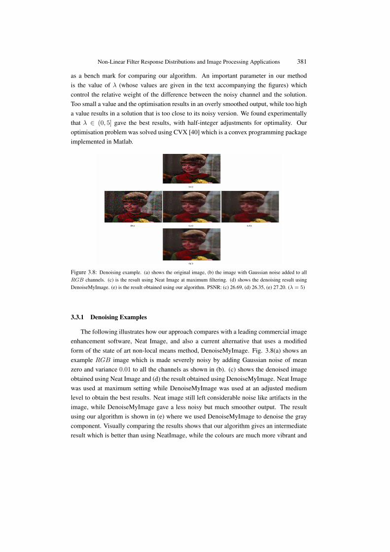
Figure 3.8: Denoising example. (a) shows the original image, (b) the image with Gaussian noise added to allRGB channels. (c) is the result using Neat Image at maximum filtering. (d) shows the denoising result usingDenoiseMyImage. (e) is the result obtained using our algorithm. PSNR: (c) 26.69, (d) 26.35, (e) 27.20. (λ = 5)

3.3.1 Denoising Examples

The following illustrates how our approach compares with a leading commercial imageenhancement software, Neat Image, and also a current alternative that uses a modifiedform of the state of art non-local means method, DenoiseMyImage. Fig. 3.8(a) shows anexample RGB image which is made severely noisy by adding Gaussian noise of meanzero and variance 0.01 to all the channels as shown in (b). (c) shows the denoised imageobtained using Neat Image and (d) the result obtained using DenoiseMyImage. Neat Imagewas used at maximum setting while DenoiseMyImage was used at an adjusted mediumlevel to obtain the best results. Neat image still left considerable noise like artifacts in theimage, while DenoiseMyImage gave a less noisy but much smoother output. The resultusing our algorithm is shown in (e) where we used DenoiseMyImage to denoise the graycomponent. Visually comparing the results shows that our algorithm gives an intermediateresult which is better than using NeatImage, while the colours are much more vibrant and


Figure 3.9: Real image denoising example. (a) is an image that has been affected by severe chroma noiseresulting in the appearance of ‘blotches’ of colour. (b) shows the denoised image obtained using Neat Imageand (c) is obtained using our algorithm. (d) is the result obtained using DenoiseMyImage. We observe thatall the reconstructions are visually similar, although on close inspection our result gives less colour aberrations.(λ = 0.5)

appear sharper than when using DenoiseMyImage. This is also further justified by the peaksignal to noise ratios (PSNR) which quantify the results, and shows our algorithm givingcomparable values.

The next examples focus on real world images where the type of noise affecting theimage is unknown. We begin with Fig. 3.9(a) which shows an image that is severely af-fected by colour noise. This is typical of an image taken in low light conditions with highISO settings. (b) shows the image having been denoised using Neat Image. This programrequires a suitable region to be selected for noise estimation, after which luminance andchrominance noise reduction can be individually adjusted. We required 100% noise reduc-tion on all components due to the high amount of noise present in the image. (c) showsour algorithm where the luminance channel was denoised using Neat Image and the filtermatrix F constructed from it for reconstructing the chroma channels. (d) shows the resultof using DenoiseMyImage. We observe that our algorithm gives similar noise reductioncompared to the existing methods, although on close inspection our result gives less colouraberrations.

Fig. 3.10(a) has been taken from some examples given on the Neat Image website. Thisis a crop of a television frame captured with a computer TV card. The image has strongcolour banding visible across all the image caused by the electric interference in the com-puter circuitry. Similar banding is sometimes observed in digital camera images (causedby interference too). The banding degradation does not affect the luminance, however allchannels still show grain like noise. (b) shows the best Neat Image result obtainable by


Figure 3.10: Real image denoising example. (a) shows an example image affected by chroma noise that appearsas bands in the colour channels. (b) is the result obtained using Neat Image which still leaves evident colourbanding. (c) is our result which is able to remove the noise leaving a clean image as the colour banding doesnot correlate with the luminance structure. (d) is the best result obtained using DenoiseMyImage. (e) shows thebanding still remaining in the V channel of the image when using Neat Image, while (e) clearly shows that thebanding structure has been removed in our reconstructed V channel. (λ = 0.1)

denoising the chroma and luminance at 100%. However, the banding is still evident in theresult. (c) is the result of our algorithm which clearly removes the noise. (d) is the bestresult obtainable using DenoiseMyImage which is still unable to remove the banding noise.

The final example illustrates the flexibility of the model in handling chroma noise takinga different distribution. Fig. 3.11 shows an image that has been corrupted by impulse noiseand reconstructed. (a) shows the original image, (b) the RGB image with noise havingbeen added to only the chroma channels and (c) shows our reconstructed image. The resultsillustrate again that noise has been successfully removed to a very high standard, and thisis further justified by looking at the chroma channels which have had their impulse noiseremoved, and by the high PSNR value. Neat Image and DenoiseMyImage are unableto satisfactorily denoise the images affected by impulse noise. They either result in theimpulse points still remaining or a ‘washed out’ look at high rates of chroma filteringe.g. (d). Interestingly, the results here indicate that given an impulse noisy colour image,concentration of noise removal in the gray image easily allows high levels of noise removalin the colour channels.


Figure 3.11: Impulse noise removal example. (a) shows an original colour image and (b) a noisy version thathas had impulse noise added to the chroma channels in the Y UV space. (c) is our reconstructed image which isvirtually identical to the original. (d) shows a typical example when using Neat Image which results in a washedout look and impulse points still visible. The impulse noise affecting the chroma is illustrated by (e) while thesuccess of our technique is shown by (f). PSNR: (c) 42.20. (λ = 0.5)

4 Conclusion

In this article we have presented some statistics concerning natural colour images andtheir applications in image processing. We have observed the sparse behaviour of the non-linear filter response distributions on natural colour images, and modeled it using a gen-eralised Gaussian distribution which generally takes shape parameter α < 1. This hasbeen empirically justified using diverse datasets of images captured using different modes.Subsequently, we incorporated knowledge of the image statistics into Bayesian models totackle several problems in image processing. Namely, colorizing gray images, compressingchroma channels and denoising colour images.

In future we will look to methods to solve the optimisation problems much faster, andat larger scales, as generally the schemes can take several minutes to solve an image ofapproximate size 250×250 pixels. We also hope to apply our work to the compression anddenoising of image streams from hyperspectral cameras which generate much higher datarate than can be accommodated by many applications.


Table 4.1: Here we show the statistics of the non-linear filter response for the sample images using the firstweighting function (2.2). α is the shape parameter of the GGD fitting and k is the kurtosis of the filter responsewith subscript notation representing the U or V component parameters.

Image U filtered response V filtered responseαU kU αV kV

balloons 0.695 11.23 0.624 14.23indoors 1.11 5.22 0.619 14.45houses 0.624 14.18 0.633 13.74

sky 0.344 94.00 0.328 114.87objects 0.54 20.35 0.662 12.43seaside 0.539 20.44 0.491 26.60night 0.944 6.52 0.561 18.37nature 0.745 9.76 0.826 8.11

Table 4.2: Statistics of the non-linear filter response for our sample images using the second weighting function(2.3).

Image U filtered response V filtered responseαU kU αV kV

balloons 0.685 11.57 0.624 14.19indoors 1.094 5.31 0.599 15.62houses 0.61 14.98 0.607 15.14

sky 0.339 99.38 0.321 126.27objects 0.534 21.02 0.654 12.79seaside 0.54 20.39 0.489 26.84night 0.931 6.66 0.556 18.85nature 0.736 10.00 0.811 8.37

Acknowledgments

This work was supported in part by grants from EPSRC and Hewlett Packard Labsawarded through the Smith Institute Knowledge Transfer Network.

References

[1] Field, D.J.: Relations between the Statistics of Natural Images and the ResponseProperties of Cortical Cells, J. Opt. Amer., Vol. 4, no. 12, pp. 2379-2394, 1987.


[2] Mallat, S.G.: A Theory for Multiresolution Signal Decomposition: The Wavelet Rep-resentation, IEEE Trans. Pattern Anal. Machine Intell., vol 11, pp. 674-693, July1989.

[3] J. Huang and D. Mumford, Statistics of Natural Images and Models, Proc. IEEECVPR, vol. 1, Fort Collins, CO, pp. 541-547 (1999).

[4] D.L. Ruderman, The statistics of natural images, Network, Vol. 5, pp. 517548, 1994.

[5] E.P. Simoncelli and E.H. Adelson, Noise removal via Bayesian wavelet coring, inThird Intl. Conf on Image Proc., Lausanne, IEEE Sig Proc Society, 1996, Vol. I, pp.379382.

[6] P. Moulin and J. Liu, Analysis of multiresolution image denoising schemes using ageneralized Gaussian and complexity priors, IEEE Trans. Info. Theory, Vol. 45, pp.909919, 1999.

[7] M.J.Wainwright and E.P. Simoncelli, Scale mixtures of Gaussians and the statisticsof natural images, Advances in Neural Information Processing Systems, S.A. Solla,T.K. Leen, and K.-R. Muller (Eds.), 2000, pp. 855861.

[8] A. Srivastava, A. B. Lee, E. P. Simoncelli, S.-C. Zhu, On Advances in StatisticalModeling of Natural Images, Journal of Mathematical Imaging and Vision archive,Volume 18, Pages: 17 - 33, 2003.

[9] D.L. Ruderman and W. Bialek: Scaling of natural images: Scaling in the woods,Physical Review Letters, Vol. 73, No. 6, pp. 814-817, 1994.

[10] S.C. Zhu and D. Mumford, Prior learning and Gibbs reactiondiffusion, IEEE Trans.Pattern Analysis and Machine Intelligence, Vol. 19, No. 11, pp. 12361250, 1997.

[11] D.L. Ruderman, Origins of scaling in natural images, Vision Research, Vol. 37, No.23, pp. 33853398, 1997.

[12] A. B. Lee, D. Mumford, J. Huang, Occlusion models for natural images: A statisticalstudy of a scale-invariant dead leaves model, International Journal of Computer Visionarchive, Volume 41 , Issue 1-2, Pages: 35 - 59, 2001.

[13] D.W. Dong and J.J. Atick, Temporal decorrelation-a theory of lagged and nonlaggedresponses in the lateral geniculate nucleus, Network, 6, 159-178, 1995.

[14] A.J. Bell, and T. J. Sejnowski, The independent components of natural scenes are edgefilters, Vision Research, Volume 37, Issue 23, December 1997, Pages 3327-3338.


[15] B. A. Olshausen and D. J. Field, Emergence of simple-cell receptive field propertiesby learning a sparse code for natural images, Nature 381, 607609, 1996.

[16] R. Linsker, Sensory processing and information theory. In Grassberger, P. and Naadal,J.P. (Eds), From statistical physics to statistical inference and back, pp 237-247. Dor-drecht: Kluwer.

[17] A. Levin, R. Fergus, F. Durand, W.T. Freeman, W.T, Image and Depth from a Conven-tional Camera with a Coded Aperture, ACM Transactions on Graphics, SIGGRAPH2007 Conference Proceedings, San Diego, 2007.

[18] M. F. Tappen, B. C. Russel, W. T. Freeman, ”Exploiting the sparse derivative prior forsuper-resolution and image demosaicing”, Proc. IEEE Workshop on Statistical andComputational Theories of Vision, 2003.

[19] A. Balinsky and N. Mohammad, Non-linear filter response distributions of naturalcolour images. LNCS 5646, pp. 101-108. Springer-Verlag Berlin Heidelberg 2009.

[20] U. Grenander and A. Srivastava, Probability Models for clutter in natural images.IEEE transactions PAMI, 23:424-429, 2001.

[21] A. Balinsky and N. Mohammad, Colorization of natural images via L1 optimization,Proc. WACV, 2009 IEEE Winter Vision Meetings, Snowbird, Utah.

[22] A. Balinsky and N. Mohammad, Sparse natural image statistics and their applicationsto colorization and compression, Proc. International Conference on Image Processs-ing (ICIP), 2010, Hong Kong.

[23] A. Balinsky and N. Mohammad, Chroma reconstruction from inaccurate measure-ments, Proceedings of the 19th International Conference on Computer Graphics, Vi-sualization and Computer Vision, Jan 2011, Plzen, Czech Republic.

[24] S. Geman, and D. Geman, Stochastic relaxation, Gibbs distributions, and the Bayesianrestoration of images. IEEE Trans. Pattern Analysis and Machine Intelligence 6: 721-741. 1984.

[25] A. Torralba, A. Oliva, Statistics of natural image categories, Network. 2003Aug;14(3):391-412.

[26] Srivastava, A.: Stochastic Models for Capturing Image Variability, IEEE Signal Pro-cesing Magazine, Volume: 19, Issue: 5 On page(s): 63-76, 2002.

[27] A. Balinsky, H. Balinsky and S. Simske, On Helmholtz’s principle for Document Pro-cessing, 10th ACM Symposium on Document Engineering (DocEng2010), Manch-ester, UK, 21-24 September 2010.


[28] A. Levin, D. Lischinski, Y. Weiss. “Colorization using optimization.” ACM Transac-tions on Graphics, Volume 23, Issue 3, pp. 689694, 2004.

[29] Caselles, V., Coll, B., Morel, J.M.: Geometry and color in natural images, J. of Math.Imaging and Vision, Volume 16, Issue 2 (March 2002), Pages: 89-105.

[30] E. Candes, “Compressive Sampling,” Int. Congress of Mathematics, 3, pp. 1433-1452,Madrid, Spain, 2006.

[31] Y. Zhang.: Solving large-scale linear programs by interior-point methods under theMATLAB environment. Optim. Methods Software 10, 1-31 (1998).

[32] S. Brooks, I. Saunders, N. A.Dodgson, “Image compression using sparse coloursampling combined with non-linear image processing,”Proc. of SPIE, Vol.6492,pp.64920F (2007).

[33] Y. Li, M. Lizhuang, W. Di, “Fast Colorization Using Edge and Gradient Constrains,”Proc. of WSCG’07, pp. 309-315.

[34] T. Horiuchi, S. Tominaga, Color image coding by colorization approach, J. on Imageand Video Proceess., Vol. 2008 , Issue 2 (Feb. 2008), Article No. 18.

[35] R. Berinde and Piotr Indyk, “Sparse recovery using sparse random matrices,”{preprint} (2008).

[36] K. Dabov, A. Foi, V. Katkovnik, and K. Egiazarian, “Color image denoising via sparse3d collaborative filtering with grouping constraint in luminance-chrominance space”,ICIP 2007. (Matlab code available at www.cs.tut.fi/foi/GCF-BM3D).

[37] A. Foi, V. Katkovnik, and V. Egiazarian, “Pointwise Shape-Adaptive DCT for High-Quality Denoising and Deblocking of Grayscale and Color Images”, IEEE Trans.Image Process., vol. 16, no. 5, May 2007.

[38] D Borkowski, “Chromaticity Denoising using Solution to the Skorokhod Problem”,Image Processing Based on Partial Differential Equations, Proceedings of the Inter-national Conference on PDE-Based Image Processing and Related Inverse Problems,CMA, Oslo, August 812, 2005.

[39] T. F. Chan and S. Esedoglu, “Aspects of total variation regularized L1 function ap-proximation”, SIAM J. Appl. Math., 65 (2005), pp. 18171837.

[40] M. Grant and S. Boyd, http://cvxr.com/cvx/


Alexander Balinsky received the PhD degree in Math-ematical Physics from the Landau Institute of TheoreticalPhysics in 1990 and was Research Fellow in the Departmentof Mathematics at The Technion-Israel Institute of Technologyfrom 1993 till 1997. He joined Cardiff University in 1997.He is a Professor in the Cardiff School of Mathematics andWIMCS Chair in Mathematical Physics. His current researchinterests lie in the areas of spectral theory, stability of matter,image processing and machine learning.

Nassir Mohammad obtained his PhD (2011) jointlywith Cardiff University and HP Labs, Bristol, UK. He ob-tained an MSc from Swansea University in Mathematicsand Computing (2006), and his BSc from Cardiff Univer-sity in Mathematics (2005). His research interests are inthe areas of analysis, image processing, statistics, proba-bility theory, machine learning and compressive sensing.Currently, he is starting a research position at HP Labs inBristol, UK.

non-linear filter response distributions of natural images

Documents