non-linear dynamics of a hanging rope - scielo · non-linear dynamics of a hanging rope . 1...

10(2013) 81 – 90

Latin American Journal of Solids and Structures 10(2013) 81 – 90

Abstract

Two-dimensional motion of a hanging rope is considered.

A multibody system with elastic-dissipative joints is used for

modelling of the rope. The mathematical model based on the

Lagrange formalism is presented. Results of some numerical simu-

lations are shown for the mechanical system with kinematic exci-

tation. Basic tools are used to qualify dynamics of the rope: the

maximum Lyapunov exponent (MLE) is estimated numerically

by the two-particle method, frequency spectra are generated via

the Fast Fourier Transform (FFT) and bifurcation diagrams are

produced. Influence of the excitation amplitude and frequency as

well as damping on behaviour of the system is analyzed. The

work can be treated as the first step in more advanced analysis of

regular and chaotic motion of the complex system.

Keywords

ropes, chains, modelling, discrete systems, non-linear dynamics,

chaos, bifurcations.

Non-linear dynamics of a hanging rope

1 INTRODUCTION

Similar to pendula, hanging ropes and chains are not only classical mechanical systems, but also

have various engineering applications. For instance, a chain can be a part of an impact damper

used for reducing wind-induced vibration of tower and mast structures [1, 2]. Moreover, the slen-

der bodies (like cables, belts, textile threads) have many features in common and simplified mod-

els of the ropes and chains can be useful to explain some interesting phenomena occurring in real

technical systems. One such example is dynamics of marine cables, particularly non-stationary

motion of a steering cable of a remotely operated underwater vehicles [8, 9]. Simulations play

even more important role in context of satellite tethers, whose motion can be hardly studied ex-

perimentally [8]. What is more, the same purely mechanical models at small length scales are

sometimes used to investigate behaviour of biological filaments and molecules such as DNA [9].

Modelling of a rope which undergoes large deformations seems to be a non-trivial task. Even if

the slender body is approximated with a discrete system, performing simulation of its motion

requires rather sophisticated numerical apparatus due to nonlinear nature of the model. However,

the discrete systems can be very attractive to researchers in the field of nonlinear dynamics. For

example, the chain-like models presented in [3, 4] are composed of many rigid links connected by

P. Fritzkowski*, H. Kaminski

Institute of Applied Mechanics, Poznan University of Technology,

24 Jana Pawla II Street, 60-965 Poznan, Poland

* Author email: [email protected]

82 P. Fritzkowski and H. Kaminski / Non-linear dynamics of a hanging rope


joints of different types. The character of the system leads to mass coupling between particular

elements. Such complex mechanical systems are rarely discussed in literature. Usually authors

focus mostly on simple systems with one, two or three degrees of freedom (e.g. see [2, 7]).

In what follows, behaviour of the rope subjected to kinematic excitation is analyzed, with use

of the mentioned discrete model. It is shown that regular and irregular motion of the system can

be observed, when values of the excitation parameters are altered. In the numerical studies, the

largest Lyapunov exponent and frequency spectra are used to identify vibration character.

2 MATHEMATICAL MODEL

The discrete model of the rope is briefly described below. Consider a uniform rope of length L and

mass M suspended from a support. For simplicity, only plane motion of the body in gravitational

field is studied. The rope itself can be modelled as a discrete system composed of n identical rigid

members, which are connected by rotational joints (see Fig. 1). Assume that the elements are

prismatic rods of length nLl / and mass nMm / . The joints, in turn, determine viscoelastic

character of the system. As a simple combination of a spring and damper, each joint is described

by stiffness Tk and damping coefficient c. The rope may be subjected to kinematic excitation

realized by the movable support, whose position depends explicitly on time:

)(00 txx , )(00 tyy . (1)

a) b)

Figure 1 Discrete model of the rope: a) general idea, b) system with elastic-dissipative joints

Using the angular generalized coordinates T21 ],,,[ n q and applying the Lagrange for-

mulation, one can obtain the following equations of motion:

P. Fritzkowski and H. Kaminski / Non-linear dynamics of a hanging rope 83


,,,2,1,1

sincos)sin()cos(

DTG

2

001

2

1

niQQQml

yxl

baa

iii

iii

n

jjijij

n

jjijij

(2)

where the coefficients ija and ib . The generalized forces on the right-hand side have

different nature: GiQ are potential forces which come from gravity; T

iQ denotes potential elastic

forces of nonlinear form, derived by applying the classical ‘bending moment – curvature’ relation-

ship for beams [4]; DiQ are dissipative forces, obtained with use of the viscous damping model [4].

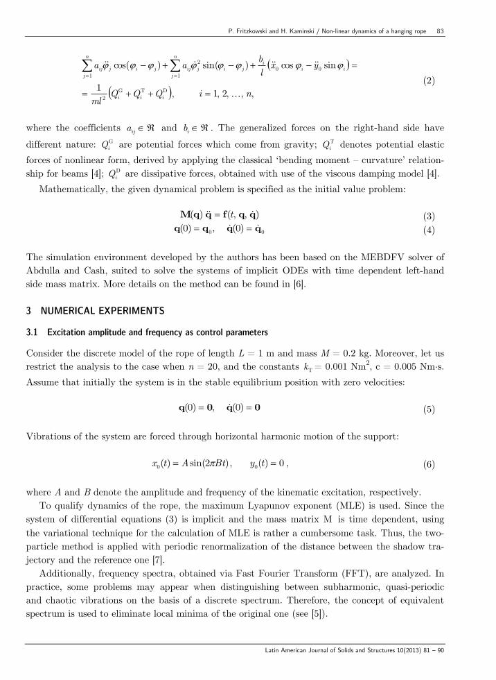
Mathematically, the given dynamical problem is specified as the initial value problem:

),,()( qqfqqM t (3)

00 )0(,)0( qqqq (4)

The simulation environment developed by the authors has been based on the MEBDFV solver of

Abdulla and Cash, suited to solve the systems of implicit ODEs with time dependent left-hand

side mass matrix. More details on the method can be found in [6].

3 NUMERICAL EXPERIMENTS

3.1 Excitation amplitude and frequency as control parameters

Consider the discrete model of the rope of length L = 1 m and mass M = 0.2 kg. Moreover, let us

restrict the analysis to the case when n = 20, and the constants Tk = 0.001 Nm2, c = 0.005 Nm·s.

Assume that initially the system is in the stable equilibrium position with zero velocities:

0q0q )0(,)0( (5)

Vibrations of the system are forced through horizontal harmonic motion of the support:

)2sin()(0 BtAtx , 0)(0 ty , (6)

where A and B denote the amplitude and frequency of the kinematic excitation, respectively.

To qualify dynamics of the rope, the maximum Lyapunov exponent (MLE) is used. Since the

system of differential equations (3) is implicit and the mass matrix M is time dependent, using

the variational technique for the calculation of MLE is rather a cumbersome task. Thus, the two-

particle method is applied with periodic renormalization of the distance between the shadow tra-

jectory and the reference one [7].

Additionally, frequency spectra, obtained via Fast Fourier Transform (FFT), are analyzed. In

practice, some problems may appear when distinguishing between subharmonic, quasi-periodic

and chaotic vibrations on the basis of a discrete spectrum. Therefore, the concept of equivalent

spectrum is used to eliminate local minima of the original one (see [5]).



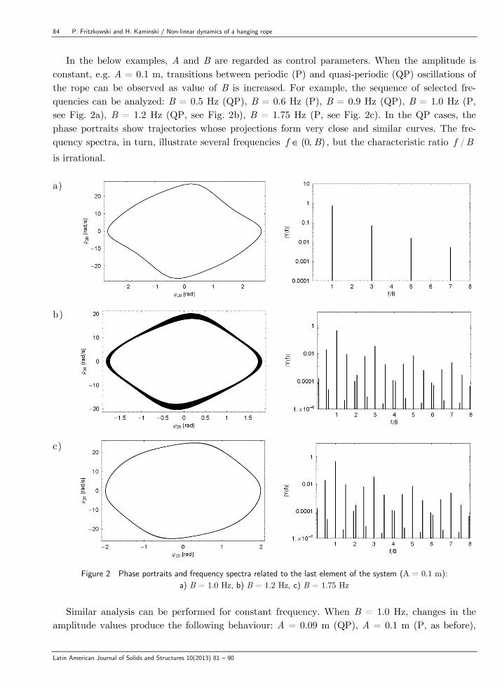
In the below examples, A and B are regarded as control parameters. When the amplitude is

constant, e.g. A = 0.1 m, transitions between periodic (P) and quasi-periodic (QP) oscillations of

the rope can be observed as value of B is increased. For example, the sequence of selected fre-

quencies can be analyzed: B = 0.5 Hz (QP), B = 0.6 Hz (P), B = 0.9 Hz (QP), B = 1.0 Hz (P,

see Fig. 2a), B = 1.2 Hz (QP, see Fig. 2b), B = 1.75 Hz (P, see Fig. 2c). In the QP cases, the

phase portraits show trajectories whose projections form very close and similar curves. The fre-

quency spectra, in turn, illustrate several frequencies ),0( Bf , but the characteristic ratio Bf /

is irrational.

a)

b)

c)

Figure 2 Phase portraits and frequency spectra related to the last element of the system (A = 0.1 m):

a) B = 1.0 Hz, b) B = 1.2 Hz, c) B = 1.75 Hz

Similar analysis can be performed for constant frequency. When B = 1.0 Hz, changes in the

amplitude values produce the following behaviour: A = 0.09 m (QP), A = 0.1 m (P, as before),



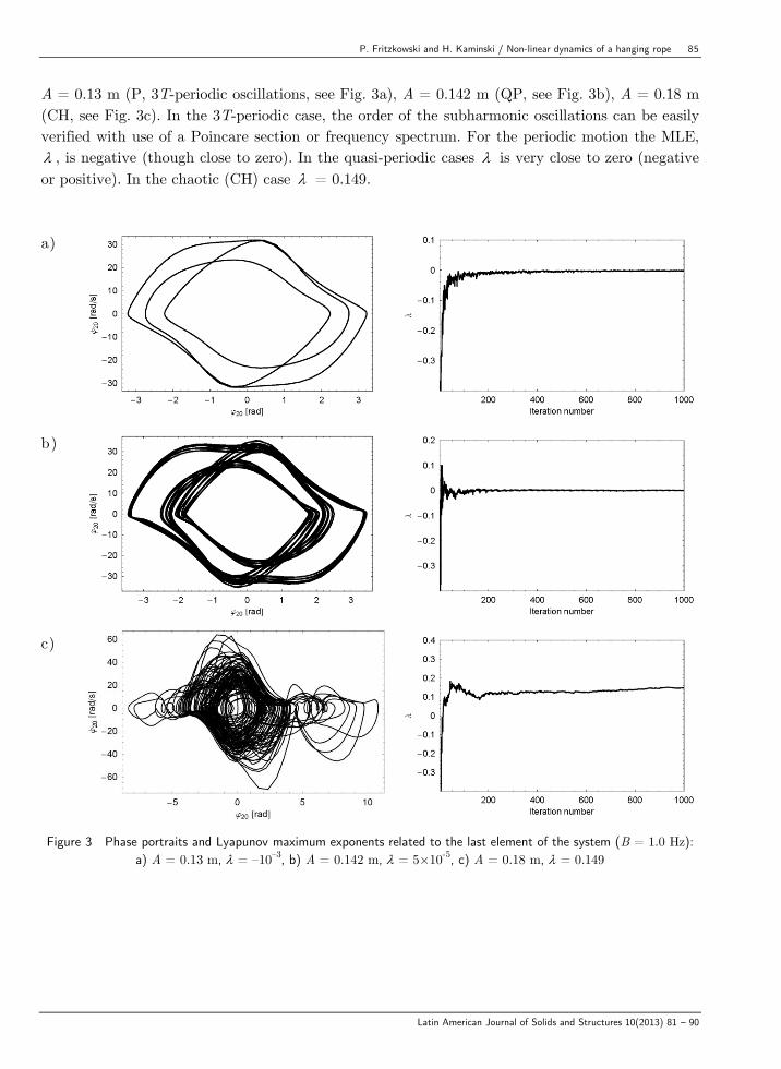
A = 0.13 m (P, 3T-periodic oscillations, see Fig. 3a), A = 0.142 m (QP, see Fig. 3b), A = 0.18 m

(CH, see Fig. 3c). In the 3T-periodic case, the order of the subharmonic oscillations can be easily

verified with use of a Poincare section or frequency spectrum. For the periodic motion the MLE,

, is negative (though close to zero). In the quasi-periodic cases is very close to zero (negative

or positive). In the chaotic (CH) case = 0.149.

a)

b)

c)

Figure 3 Phase portraits and Lyapunov maximum exponents related to the last element of the system (B = 1.0 Hz):

a) A = 0.13 m, = –10–3

, b) A = 0.142 m, = 5×10-5, c) A = 0.18 m, = 0.149



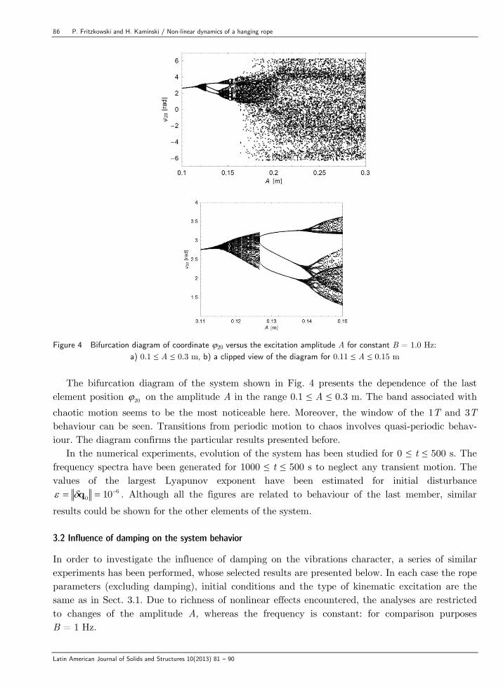
Figure 4 Bifurcation diagram of coordinate 20 versus the excitation amplitude A for constant B = 1.0 Hz:

a) 0.1 ≤ A ≤ 0.3 m, b) a clipped view of the diagram for 0.11 ≤ A ≤ 0.15 m

The bifurcation diagram of the system shown in Fig. 4 presents the dependence of the last

element position 20 on the amplitude A in the range 0.1 ≤ A ≤ 0.3 m. The band associated with

chaotic motion seems to be the most noticeable here. Moreover, the window of the 1T and 3T

behaviour can be seen. Transitions from periodic motion to chaos involves quasi-periodic behav-

iour. The diagram confirms the particular results presented before.

In the numerical experiments, evolution of the system has been studied for 0 ≤ t ≤ 500 s. The

frequency spectra have been generated for 1000 ≤ t ≤ 500 s to neglect any transient motion. The

values of the largest Lyapunov exponent have been estimated for initial disturbance 6

0 10 q . Although all the figures are related to behaviour of the last member, similar

results could be shown for the other elements of the system.

3.2 Influence of damping on the system behavior

In order to investigate the influence of damping on the vibrations character, a series of similar

experiments has been performed, whose selected results are presented below. In each case the rope

parameters (excluding damping), initial conditions and the type of kinematic excitation are the

same as in Sect. 3.1. Due to richness of nonlinear effects encountered, the analyses are restricted

to changes of the amplitude A, whereas the frequency is constant: for comparison purposes

B = 1 Hz.



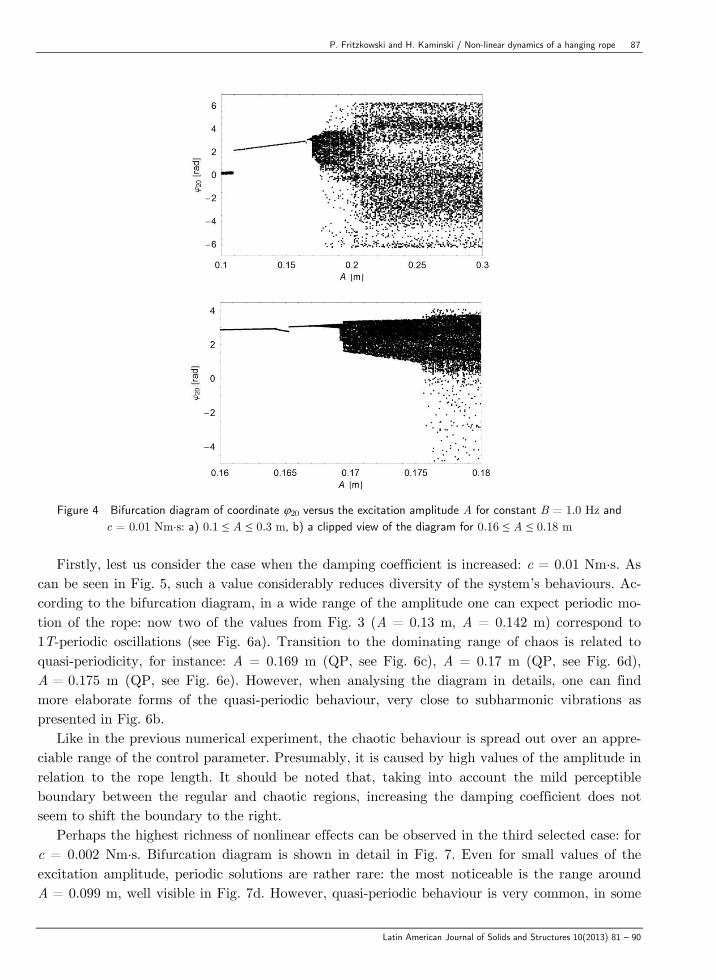
Figure 4 Bifurcation diagram of coordinate 20 versus the excitation amplitude A for constant B = 1.0 Hz and

c = 0.01 Nm·s: a) 0.1 ≤ A ≤ 0.3 m, b) a clipped view of the diagram for 0.16 ≤ A ≤ 0.18 m

Firstly, lest us consider the case when the damping coefficient is increased: c = 0.01 Nm·s. As

can be seen in Fig. 5, such a value considerably reduces diversity of the system’s behaviours. Ac-

cording to the bifurcation diagram, in a wide range of the amplitude one can expect periodic mo-

tion of the rope: now two of the values from Fig. 3 (A = 0.13 m, A = 0.142 m) correspond to

1T-periodic oscillations (see Fig. 6a). Transition to the dominating range of chaos is related to

quasi-periodicity, for instance: A = 0.169 m (QP, see Fig. 6c), A = 0.17 m (QP, see Fig. 6d),

A = 0.175 m (QP, see Fig. 6e). However, when analysing the diagram in details, one can find

more elaborate forms of the quasi-periodic behaviour, very close to subharmonic vibrations as

presented in Fig. 6b.

Like in the previous numerical experiment, the chaotic behaviour is spread out over an appre-

ciable range of the control parameter. Presumably, it is caused by high values of the amplitude in

relation to the rope length. It should be noted that, taking into account the mild perceptible

boundary between the regular and chaotic regions, increasing the damping coefficient does not

seem to shift the boundary to the right.

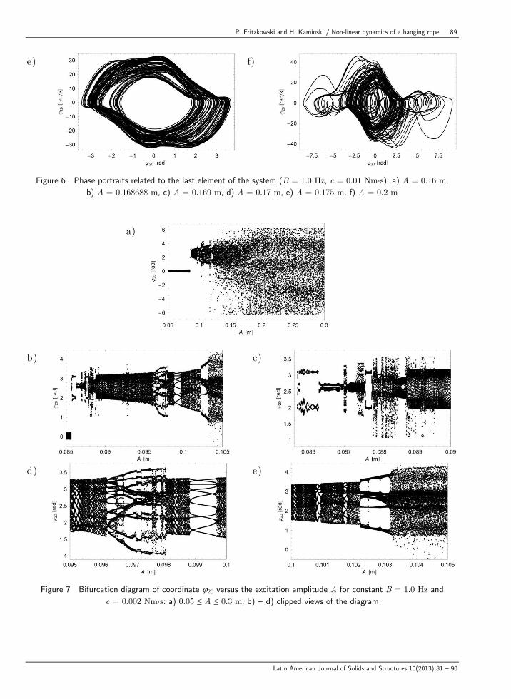
Perhaps the highest richness of nonlinear effects can be observed in the third selected case: for

c = 0.002 Nm·s. Bifurcation diagram is shown in detail in Fig. 7. Even for small values of the

excitation amplitude, periodic solutions are rather rare: the most noticeable is the range around

A = 0.099 m, well visible in Fig. 7d. However, quasi-periodic behaviour is very common, in some



ranges it seems very similar to subharmonic vibrations. The chaotic region, in turn, is moved to

the left.

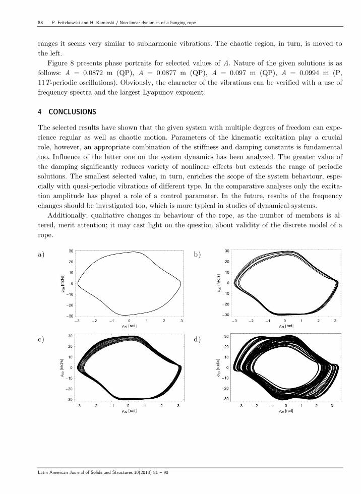
Figure 8 presents phase portraits for selected values of A. Nature of the given solutions is as

follows: A = 0.0872 m (QP), A = 0.0877 m (QP), A = 0.097 m (QP), A = 0.0994 m (P,

11T-periodic oscillations). Obviously, the character of the vibrations can be verified with a use of

frequency spectra and the largest Lyapunov exponent.

4 CONCLUSIONS

The selected results have shown that the given system with multiple degrees of freedom can expe-

rience regular as well as chaotic motion. Parameters of the kinematic excitation play a crucial

role, however, an appropriate combination of the stiffness and damping constants is fundamental

too. Influence of the latter one on the system dynamics has been analyzed. The greater value of

the damping significantly reduces variety of nonlinear effects but extends the range of periodic

solutions. The smallest selected value, in turn, enriches the scope of the system behaviour, espe-

cially with quasi-periodic vibrations of different type. In the comparative analyses only the excita-

tion amplitude has played a role of a control parameter. In the future, results of the frequency

changes should be investigated too, which is more typical in studies of dynamical systems.

Additionally, qualitative changes in behaviour of the rope, as the number of members is al-

tered, merit attention; it may cast light on the question about validity of the discrete model of a

rope.

a)

b)

c)

d)



e)

f)

Figure 6 Phase portraits related to the last element of the system (B = 1.0 Hz, c = 0.01 Nm·s): a) A = 0.16 m,

b) A = 0.168688 m, c) A = 0.169 m, d) A = 0.17 m, e) A = 0.175 m, f) A = 0.2 m

a)

b)

c)

d)

e)

Figure 7 Bifurcation diagram of coordinate 20 versus the excitation amplitude A for constant B = 1.0 Hz and

c = 0.002 Nm·s: a) 0.05 ≤ A ≤ 0.3 m, b) – d) clipped views of the diagram



a)

b)

c)

d)

Figure 8 Phase portraits related to the last element of the system (B = 1.0 Hz, c = 0.002 Nm·s):

a) A = 0.0872 m, b) A = 0.0877 m, c) A = 0.097 m, d) A = 0.0994 m

Thus, the work can be treated as the first step to consider bifurcations of the system and to

study its nonlinear dynamics in a more systematic way, with use of the advanced numerical tools.

Acknowledgements

The paper has been presented during 11th Conference on Dynamical Systems – Theory and Ap-

plications. This work has been supported by 21-381/2012 DS grant.

References

[1] Koss L.L., Melbourne W.H., Chain dampers for control of wind-induced vibration of tower and mast struc-

tures. Engineering Structures, 17(9), 1995, 622-625.

[2] Sado D., Regular and Chaotic Vibrations of Selected Systems with Pendula. Warsaw, WNT, 2010 [in Polish].

[3] Fritzkowski P., Kaminski H., Dynamics of a rope as a rigid multibody system. Journal of Mechanics of Mate-

rials and Structures, 3(6), 2008, 1059-1075.

[4] Fritzkowski P., Kaminski H., A discrete model of a rope with bending stiffness or viscous damping. Acta

Mechanica Sinica, 27(1), 2011, 108-113.

[5] Luczko J., Regular and Chaotic Vibrations in Nonlinear Mechanical Systems. Krakow, Publishing House of

Krakow University of Technology, 2008 [in Polish].

[6] Cash J.R., Considine S., An MEBDF code for stiff initial value problems. ACM Transactions on Mathematical

Software, 18(2), 1992, 142-155.

[7] Awrejcewicz J., Kudra G., Lamarque C.-H., Investigation of triple pendulum with impacts using fundamental

solution matrices. International Journal of Bifurcation and Chaos in Applied Sciences and Engineering, 14(12),

2004, 4191-4213.

[8] Weiss H., Dynamics of Geometrically Nonlinear Rods: II. Numerical Methods and Computational Examples.

Nonlinear Dynamics, 30(4), 2002, 383-415.

[9] Goyal S., Perkins N.C., Lee C.L., Nonlinear dynamics and loop formation in Kirchhoff rods with implications

to the mechanics of DNA and cables. Journal of Computational Physics, 209, 2005, 371-389.

non-linear dynamics of a hanging rope - scielo · non-linear dynamics of a hanging rope . 1...

Documents