nomenclature - d1rkab7tlqy5f1.cloudfront.net scie… · nomenclature roman symbols symbol...
TRANSCRIPT

Nomenclature
Roman Symbols
Symbol Description S.I. units
A Surface of the cross-section (m2)
Ap Area of measurement volume projection (m2)
CL Relative change of measurement volume position
in water (m)
D Diameter of cylindrical tube (m)
De2 Diameter of laser beam (m)
Dh Hydraulic diameter (m)
H Height of fluid-flow step (m)
I Relative light intensity (m−2)
Jk Variance estimation for slot (-)
L Characteristic length scale (m)
L Reattachment length after fluid-flow step (m)
Lz Large scale coherent structure length (m)
M Average particle concentration (m−3)
N Counting integer (-)
Ruu Autocorrelation (-)ˆRu′u′ Estimated autocorrelation (-)
S Radiant sensitivity constant (-)
S Perimeter of tube (m)
Tλ Taylor time scale (s)
U Wetted perimeter (m)~U Fluid velocity (m/s)~V Fluid velocity (m/s)
V ∗ Friction velocity (m/s)
V + Velocity normalized by the friction velocity (-)~W Fluid velocity (m/s)
ai Amplitude of refracted beam (-)
bk Slot interval (-)
c Speed of light (m /s)
d Distance between incident beams (m)
df Fringe pattern distance (m)
dm Width of measurement volume (m)
dp Particle diameter (m)
v

vi
~e Unit vector (-)
~es Direction of detector (-)
f Focal length of lens (m)
f LDA data rate (s−1)
f0 Source frequency (s−1)
fs Frequency scattered toward detector (s−1)
fD Doppler shift frequency (s−1)
hm Height of measurement volume (m)
k Counting integer (m)
lm Length of measurement volume (m)
ni Refractive index of substance i (-)
p Pressure (kg/m3)
p Density function (-)
~r Angular distance (m)
sij Strain rate tensor (1 / s)
t Time (s)
tr Residence time of particle in measurement volume (s)
uη Kolmogorov veloity scale (m/s)
u′ Fluid velocity fluctuation (m / s)
u Time averaged velocity (m /s)
ui Velocity-component in direction i (m / s)
v Velocity component (m/s)
v∗ Friction velocity (m/s)
v+ Non-dimensional fluid velocity (-)
y+ Non-dimensional wall distance (-)
Greek Symbols
Symbol Description S.I. units
∆t Interarrival time (s)
∆τ Time lag (s)
Φ External force on fluid flow (kg / m2 s2)
Λ Number of particles crossing the measurement volume per time (s−1)
α Angle of incident beam (-)
α Thermal expansion coefficient (m / m K)
β Angle of incident beam (-)
ǫ Dissipation rate (m2 / s3)
φ Phase (-)
η Amplitude ratio (-)
η Kolmogorov length scale (m)
κ Angle of incident beam (-)
λ Mean number of samples per unit time (s−1)
λ Taylor lentgh scale (m)
λ0 Wavelength of incident light (m)
µ Dynamic viscosity (kg / m s)

vii
ν Kinematic viscosity (m2 / s)
ν Data rate (s−1)
σ Standard deviation (-)
ρ Density ( kgm3 )
ρf Fluid density ( kgm3 )
ρk Correlation function (-)
ρp Particle density ( kgm3 )
τ Dissipative time scale of turbulence (s)
τ Correlation time lag (s)
τc Coincidence windows width (s)
τ Projection of the Reynols stress tensor on the
cross-section of the pipe (kg / ms2)
τi Deviatoric part of the Reynolds stress tensor (kg / ms2)
τk Average time lag per bin (s)
τd Isotropic part of the Reynolds stress tensor (kg / m s2)
τw Wall shear stress (kg / s 2)
θ Angle of incidence or refraction (-)
ω Angular frequency (s−1)
Abbreviations
Abbreviation Description
ACF Auto Correlation Function
BBO Basset-Bousinesq-Oseen
FEP Fluorinated Ethylene Propylene
FFT Fast Fourier Transform
IFA Intelligent Flow Analyser
LDA Laser Doppler Anemometry
PIV Particle Image Velocimetry
PDF Probability Density Function
PMMA Poly Methyl Methacrylate
PTFE Poly Tetra Fluoro Ethylene
PVC Poly Vinyl Chloride
RMS Root Mean Square
SNR Signal to Noise Ratio
TSI Brand name
Dimensionless groups
Symbol Description
Sr Strouhal number

viii
Re Reynolds number
Contents
Abstract i
Samenvatting iii
Nomenclature v
1 Introduction 1
2 Cross flow 3
2.1 Secondary Flow . . . . . . . . . . . . . . . . . . . . . . . . . . . . . . . . . . . . . . 3
2.2 Secondary Flow in a Rod Bundle Subchannel . . . . . . . . . . . . . . . . . . . . . 6
2.3 Large scale coherent structures . . . . . . . . . . . . . . . . . . . . . . . . . . . . . 8
3 Laser Doppler Anemometry 11
3.1 Introduction to LDA . . . . . . . . . . . . . . . . . . . . . . . . . . . . . . . . . . . 11
3.2 Doppler effect . . . . . . . . . . . . . . . . . . . . . . . . . . . . . . . . . . . . . . . 12
3.3 LDA detection . . . . . . . . . . . . . . . . . . . . . . . . . . . . . . . . . . . . . . 13
3.3.1 Photo detection . . . . . . . . . . . . . . . . . . . . . . . . . . . . . . . . . . 13
3.3.2 Optical configurations . . . . . . . . . . . . . . . . . . . . . . . . . . . . . . 13
3.3.3 Fringe model . . . . . . . . . . . . . . . . . . . . . . . . . . . . . . . . . . . 14
3.3.4 Directional ambiguity . . . . . . . . . . . . . . . . . . . . . . . . . . . . . . 15
3.3.5 Measurement volume . . . . . . . . . . . . . . . . . . . . . . . . . . . . . . . 16
3.3.6 Particles . . . . . . . . . . . . . . . . . . . . . . . . . . . . . . . . . . . . . . 17
3.4 Signal processing . . . . . . . . . . . . . . . . . . . . . . . . . . . . . . . . . . . . . 18
3.4.1 Intelligent Flow Analyser . . . . . . . . . . . . . . . . . . . . . . . . . . . . 18
3.4.2 Computerised post-processing . . . . . . . . . . . . . . . . . . . . . . . . . . 19
3.5 LDA configuration . . . . . . . . . . . . . . . . . . . . . . . . . . . . . . . . . . . . 19
3.5.1 Laser . . . . . . . . . . . . . . . . . . . . . . . . . . . . . . . . . . . . . . . 20
3.5.2 Colorburst . . . . . . . . . . . . . . . . . . . . . . . . . . . . . . . . . . . . 20
3.5.3 Probe . . . . . . . . . . . . . . . . . . . . . . . . . . . . . . . . . . . . . . . 20
3.5.4 Colorlink . . . . . . . . . . . . . . . . . . . . . . . . . . . . . . . . . . . . . 21
3.5.5 Intelligent Flow Analyser 750 and FIND software . . . . . . . . . . . . . . . 21
3.5.6 Traversing system . . . . . . . . . . . . . . . . . . . . . . . . . . . . . . . . 22
3.5.7 Seeding particles . . . . . . . . . . . . . . . . . . . . . . . . . . . . . . . . . 22
4 Post-processing 23
4.1 Raw data . . . . . . . . . . . . . . . . . . . . . . . . . . . . . . . . . . . . . . . . . 23
4.1.1 Particle distribution . . . . . . . . . . . . . . . . . . . . . . . . . . . . . . . 23
4.1.2 Detector characteristics . . . . . . . . . . . . . . . . . . . . . . . . . . . . . 25
4.2 Calculated velocity information . . . . . . . . . . . . . . . . . . . . . . . . . . . . . 26
ix

x CONTENTS
4.2.1 Velocity profile . . . . . . . . . . . . . . . . . . . . . . . . . . . . . . . . . . 26
4.2.2 Autocorrelation function . . . . . . . . . . . . . . . . . . . . . . . . . . . . . 26
4.2.3 Stresses . . . . . . . . . . . . . . . . . . . . . . . . . . . . . . . . . . . . . . 26
4.3 Data filtering and correction . . . . . . . . . . . . . . . . . . . . . . . . . . . . . . . 27
4.3.1 Clipping . . . . . . . . . . . . . . . . . . . . . . . . . . . . . . . . . . . . . . 27
4.3.2 Multiple Validation . . . . . . . . . . . . . . . . . . . . . . . . . . . . . . . . 27
4.3.3 Coincidence window . . . . . . . . . . . . . . . . . . . . . . . . . . . . . . . 27
4.3.4 Velocity bias . . . . . . . . . . . . . . . . . . . . . . . . . . . . . . . . . . . 27
4.3.5 Correlation calculation . . . . . . . . . . . . . . . . . . . . . . . . . . . . . . 29
4.3.6 Model-based fitting of the correlation function . . . . . . . . . . . . . . . . 31
5 Refractive Index Matching 33
5.1 Motivation . . . . . . . . . . . . . . . . . . . . . . . . . . . . . . . . . . . . . . . . 33
5.2 Types of refractive index matching . . . . . . . . . . . . . . . . . . . . . . . . . . . 33
5.3 FEP . . . . . . . . . . . . . . . . . . . . . . . . . . . . . . . . . . . . . . . . . . . . 34
5.3.1 Optical properties . . . . . . . . . . . . . . . . . . . . . . . . . . . . . . . . 34
5.3.2 Mechanical properties . . . . . . . . . . . . . . . . . . . . . . . . . . . . . . 35
5.4 Remaining errors . . . . . . . . . . . . . . . . . . . . . . . . . . . . . . . . . . . . . 36
6 Single Phase Turbulent Pipe Flow 39
6.1 Setup . . . . . . . . . . . . . . . . . . . . . . . . . . . . . . . . . . . . . . . . . . . 39
6.2 Experimental conditions . . . . . . . . . . . . . . . . . . . . . . . . . . . . . . . . . 40
6.2.1 Fluid flow . . . . . . . . . . . . . . . . . . . . . . . . . . . . . . . . . . . . . 40
6.2.2 Measurement volume position in the tube . . . . . . . . . . . . . . . . . . . 40
6.2.3 LDA settings . . . . . . . . . . . . . . . . . . . . . . . . . . . . . . . . . . . 40
6.3 Results . . . . . . . . . . . . . . . . . . . . . . . . . . . . . . . . . . . . . . . . . . . 43
6.3.1 Parallel profile . . . . . . . . . . . . . . . . . . . . . . . . . . . . . . . . . . 43
6.3.2 Perpendicular profile . . . . . . . . . . . . . . . . . . . . . . . . . . . . . . . 44
6.3.3 Discussion . . . . . . . . . . . . . . . . . . . . . . . . . . . . . . . . . . . . . 44
7 Rod Bundle Flow 49
7.1 Experimental Setup . . . . . . . . . . . . . . . . . . . . . . . . . . . . . . . . . . . 49
7.1.1 Design constraints . . . . . . . . . . . . . . . . . . . . . . . . . . . . . . . . 49
7.1.2 Rod bundle flow loop . . . . . . . . . . . . . . . . . . . . . . . . . . . . . . 50
7.1.3 Inflow section . . . . . . . . . . . . . . . . . . . . . . . . . . . . . . . . . . . 50
7.1.4 General sections . . . . . . . . . . . . . . . . . . . . . . . . . . . . . . . . . 52
7.1.5 Measurement section . . . . . . . . . . . . . . . . . . . . . . . . . . . . . . . 53
7.1.6 Outflow section . . . . . . . . . . . . . . . . . . . . . . . . . . . . . . . . . . 54
7.1.7 Tubes and spacers . . . . . . . . . . . . . . . . . . . . . . . . . . . . . . . . 54
7.2 Experimental conditions . . . . . . . . . . . . . . . . . . . . . . . . . . . . . . . . . 56
7.3 Quality of the setup . . . . . . . . . . . . . . . . . . . . . . . . . . . . . . . . . . . 59
7.3.1 Positions of tubes . . . . . . . . . . . . . . . . . . . . . . . . . . . . . . . . 59
7.3.2 Allowed measurement locations . . . . . . . . . . . . . . . . . . . . . . . . . 61
7.3.3 Refractive index mismatch . . . . . . . . . . . . . . . . . . . . . . . . . . . . 62
7.4 Secondary Flow . . . . . . . . . . . . . . . . . . . . . . . . . . . . . . . . . . . . . . 65
7.5 Flow profiles . . . . . . . . . . . . . . . . . . . . . . . . . . . . . . . . . . . . . . . 65
7.5.1 Laminar . . . . . . . . . . . . . . . . . . . . . . . . . . . . . . . . . . . . . . 68
7.5.2 Turbulent . . . . . . . . . . . . . . . . . . . . . . . . . . . . . . . . . . . . . 68
7.6 Large scale coherent structures . . . . . . . . . . . . . . . . . . . . . . . . . . . . . 72
8 Conclusions and Recommendations 75

CONTENTS xi
8.1 Conclusions . . . . . . . . . . . . . . . . . . . . . . . . . . . . . . . . . . . . . . . . 75
8.2 Future work . . . . . . . . . . . . . . . . . . . . . . . . . . . . . . . . . . . . . . . . 76
8.3 Recommendations . . . . . . . . . . . . . . . . . . . . . . . . . . . . . . . . . . . . 77
8.3.1 Improvement of LDA procedure . . . . . . . . . . . . . . . . . . . . . . . . . 77
8.3.2 Rod bundle . . . . . . . . . . . . . . . . . . . . . . . . . . . . . . . . . . . . 77
Acknowledgements 79
A Microscales 81
A.1 Kolmogorov microscales . . . . . . . . . . . . . . . . . . . . . . . . . . . . . . . . . 81
A.2 Taylor microscales . . . . . . . . . . . . . . . . . . . . . . . . . . . . . . . . . . . . 82
B Friction velocity 85
C FEP: properties and treatment 87
C.1 FEP . . . . . . . . . . . . . . . . . . . . . . . . . . . . . . . . . . . . . . . . . . . . 87
C.2 Shaping by shrinking . . . . . . . . . . . . . . . . . . . . . . . . . . . . . . . . . . . 88
C.3 Mounting of FEP . . . . . . . . . . . . . . . . . . . . . . . . . . . . . . . . . . . . . 90
C.3.1 Shrinking . . . . . . . . . . . . . . . . . . . . . . . . . . . . . . . . . . . . . 90
C.3.2 Clamping . . . . . . . . . . . . . . . . . . . . . . . . . . . . . . . . . . . . . 90
D Flow transitions 93
D.1 Wires in flow . . . . . . . . . . . . . . . . . . . . . . . . . . . . . . . . . . . . . . . 93
D.2 Backward-facing step . . . . . . . . . . . . . . . . . . . . . . . . . . . . . . . . . . . 94
D.3 Forward-facing step . . . . . . . . . . . . . . . . . . . . . . . . . . . . . . . . . . . . 95
Bibliography 96

CHAPTER 1
Introduction
A vertical rod bundle geometry is characterised by cylindrical rods aligned on a rectangular grid.
The space in between the rods is filled with fluid, which flows in the axial direction of the tubes.
Figure 1.1 shows a typical rod bundle geometry. The geometrical proportions can be expressed
using the diameter to pitch ratio.
Figure 1.1: Part of an infinite rod bundle geometry, the water flows streamwise along the rods.
Major applications of rod bundle geometries can be found in heat exchangers and the core of nuclear
reactors. In these systems, the exchange of scalar quantities like heat or mass are important and
interesting and are mainly caused by fluid flow effects.
Inter channel scalar transport is enhanced by cross flow phenomena, which occur in rod bundle
flows [1, 2], and it effects the distribution of mass and/or enthalpy. Concerning flows in nuclear
reactors, the fission process depends on the water flow, temperature and accompanying density,
because water takes part in the chain reaction as moderator. The fluid flow rate on its turn is
dependent on the heat produced in the fission process. This coupling between fluid flow and nu-
clear fission underlines the importance of a full understanding of the flow effects in a rod bundle
geometry.
1

2 CHAPTER 1. INTRODUCTION
Previous research on rod bundle flow has been conducted both numerically and experimentally.
Lexmond et al. [2] investigated fluid flow in two rectangular subchannels, connected by a small gap,
using Particle Image Velocimetry (PIV): they observed alternating vortices, separated by zones of
large cross-flow. In a similar experiment with two rectangular sub-channels but now connected by
a near-wall curved gap, Mahmood et al. [1] also observed alternating vortex streets and zones of
large cross-flow.
An important issue is whether the structures measured by Lexmond et al. and Mahmood et al.
would also occur in a more complex geometry like a complete rod bundle. A full rod bundle
geometry was computed by Ikeno and Kajishima [3] using Large Eddy Simulations (LES). They
observed large scale structures covering two subchannels. Furthermore, they saw a pulsating flow
through the gaps.
As far as we know no previous experimental research has been conducted on full rod-bundle ge-
ometries, where the velocity and turbulence intensities have been measured with a high spatial
resolution. So far, only Zhang et al. [4] visualised a multi-phase rod bundle flow using a high-speed
camera.
The objective of this project is to develop an experimental technique using refractive index match-
ing with Fluorinated Ethylene Propylene (FEP). This technique will be investigated using a single
phase turbulent pipe, a well described flow situation, and in a rod bundle geometry with a diame-
ter over pitch ratio of 0.7. The possibilities and limitations of Laser Doppler Anemometry (LDA)
measurements in both flow cases will be discussed. The technique will be used to investigate the
results of the previous research in a full scale geometry.
Outline
The thesis starts with a theory on cross flow and large scale structures, in Chapter 2. The ex-
perimental technique of LDA is introduced in Chapter 3 and the postprocessing required for LDA
is treated in Chapter 4. The measurements of FEP properties with respect to refractive index
matching are discussed in Chapter 5. Results for the turbulent pipe flow case can be found in
Chapter 6 and for the rod bundle flow experiments in Chapter 7. The thesis is concluded with
conclusions and recommendations in Chapter 8

CHAPTER 2
Cross flow
This chapter describes the fluid flow in a vertical rod-bundle geometry as is explained in the
previous chapter and shown in Figure 1.1.
Two different cross flow types can be distinguished: Secondary flow, discussed in section 2.1 and
lateral flow due to large scale vortices, discussed in section2.3. The application of secondary flow
on a rod bundle geometry is treated in section 2.2.
2.1 Secondary Flow
Under certain conditions the flow of a fluid can be accompanied by secondary flow, i.e. a mean flow
perpendicular to the main flow direction. This was first discovered by Nikuradse [5] and further
discussed by Prandtl [6]. Since then, many research has been conducted on secondary flow, because
it can alter the flow significantly.
Of the different methods to analyse secondary flow, the method using the the Reynolds stresses in
the cross-section will be described in this section. This treatment is based on chapter 6 of Belt [7],
where more background information can be found as well.
The fully developed flow inside a channel can be described by the following equations:
~U = ~V + ~W
~V = vx ~ex + vy ~ey
~W = w~ez
The direction ez is in the streamwise direction and ex and ey are the two orthogonally unit vectors
in the cross-section of the channel. A graphical interpretation of the different directions can be
found in 2.1.
For the fully developed flow, the flow in the cross-section, ~V , can be described by the continuity
and Navier-Stokes equation, for this 2D situation:
3

4 CHAPTER 2. CROSS FLOW
Figure 2.1: Definition of directions in flow
∇ · ~V = 0 (2.1)
ρD~V
Dt= −∇p + µ∇2~V + ∇ · τ (2.2)
where ρ is the density, p is the projection of the pressure on the cross-section, µ is the viscosity
and τ is the projection of the Reynolds stress tensor on the cross-section of the pipe. The term
µ∇2~V is the transport caused by diffusion.
Because the average pressure in the pipe cross-section cannot drive the fluid, the secondary flow
should be generated by the divergence of τ . Since this Reynolds stress tensor does not exist in
laminar flow, secondary flow (without an external force) cannot occur in laminar flow.
The projection of the Reynolds stress tensor on the cross-section, τ , is given by (by definition):
τ = −ρ
(u′
yu′y u′
zu′y
u′yu′
z u′zu
′z
)
(2.3)
This tensor can be split into an isotropic part, (τi), and a deviatoric part (τd) according to:
τi = −ρ
(u′
yu′
y
2 0
0u′
zu′z2
)
(2.4)
τd = −ρ
(u′
yu′
y
2 u′zu
′y
u′yu′
zu′
zu′
z
2
)
(2.5)
Replacing τ in equation 2.2 gives:
ρD~v
Dt= −∇
(
p − τt
2
)
+ µ∇2~v + ∇ · τd (2.6)

2.1. SECONDARY FLOW 5
A vorticity term in the Navier-Stokes equations in the axial direction in a fully-developed pipe flow
is only non-zero if secondary flow is present [8]. Analysis of the vorticity equations is therefore
interesting and can be obtained by taking the curl of equation 2.6:
ρDω
Dt= µ∇2ω + ∇× (∇ · τ ) (2.7)
In this equation, τ can be replaced by τd, because ∇×∇τi = 0. The ρDωDt term is the transport of
vorticity by secondary flow, µ∇2ω is the diffusive term and the last term is caused by the turbulent
Reynolds stresses, which is the source of the vorticity. This last term is needed to maintain the
secondary flow. A necessary and sufficient condition is therefore:
∇× (∇ · τ ) 6= 0. (2.8)
From this equation it can be seen that the gradient should be anisotropic and not the Reynolds
stress itself. An example of this is a flow in a circular pipe, the Reynolds stress tensor itself is not
isotropic, but due to the cylindrical symmetry no secondary flow occurs.
The value of the secondary flow itself can be determined by solving equation 2.6 with the generalised
Helmholtz decomposition [7] resulting in:
~V ( ~x1) =1
2π
∫
A
~r( ~x1, ~x2)
r2( ~x1, ~x2)× ω( ~x2)~ez dA( ~x2) (2.9)
here ~x1 and ~x2 are the position vectors in the cross-section, A is the surface of the cross-section, ~r
is the distance between ~x1 and ~x2.
To calculate the secondary flow, ~V , it is needed to know ∇ cot τ as well as the projection of
the pressure gradient on the surface. This is not known beforehand and modelling of the pressure
is difficult [7], so the analytical solution is challenging.
External forces applied to the flow, like a difference in wall roughness, particles in the flow or
a body force, can introduce a secondary flow as well. Examples of body forces are gravity in
the non-streamwise direction or an electromagnetic field on a magnetic fluid. This force can be
introduced in the momentum equation as follows:
ρD~V
Dt= −∇p + µ∇2~V + ∇ · τ + ~Φ (2.10)
The external force can be enough to introduce secondary flow, even if the divergence of the Reynolds
stresses does not give rise to this. However, further treatment of this externally introduced sec-
ondary flow is beyond the scope of this thesis. More information on this can be found for example
in Daalmans [9].
Secondary flows can be subdivided into different categories, according to the source of the flow,
after Bradshaw [10]. Two commonly known types are secondary flow of Prandtl’s:
• First kind: an essentially inviscid process which is driven by the skewness of the flow, which
is caused by the geometry. The created vorticity is diffused (and therefore reduced) by the

6 CHAPTER 2. CROSS FLOW
Figure 2.2: Cross-section of a sub-channel with a square inside
Reynolds and viscous stresses. This kind can be found in laminar and turbulent flow. This
flow can be in the order of 1/10th of the main flow.
• Second kind: the vorticity is created by the Reynolds stresses. The exact mechanism is
described above. In short, it can be described as a transfer of momentum from the streamwise
direction to the cross-sectional directions by turbulence, which introduces the vorticity. This
flow is typically in the order of 1 % of the main flow.
Secondary flow of Prandtl’s second kind originates from the Reynolds stresses in the flow. The
Reynolds stresses themselves are a time-averaged correlation between various velocity components
in the fluid. This type of secondary flow therefore is an averaged fluid flow and is not recognisable
in the instantaneous velocity field.
2.2 Secondary Flow in a Rod Bundle Subchannel
It is difficult to find out secondary flow in a rod bundle subchannel analytically, since it requires
a complete analysis of the Reynolds and wall’s stresses. However, the problem can be simplified
by a square duct, as can be seen in Figure 2.2. This approximation is based on the secondary flow
patterns observed in both cases, as can be seen in Figure 2.3. This means that the equations of a
simple square duct can describe a rod bundle sub-channel.
The secondary flow of Prandtl’s second kind in a square duct is extensively described in literature.
Gessner [11] gives an analytical description combined with experimental data. The rest of this
section is based on his derivation.
Assuming that all Reynolds stress components have the same order of magnitude, the govern-
ing Reynolds equations for the flow in the corner region outside the viscous sublayer, are:

2.2. SECONDARY FLOW IN A ROD BUNDLE SUBCHANNEL 7
Figure 2.3: Comparison between secondary flow in a rod-bundle subchannel (left, Ikeno and Kajishima[3]) and secondary flow in a square duct (right, Huser and Biringen [12])
U∂U
∂x+ V
∂U
∂y+ W
∂U
∂z= −1
ρ
∂p
∂x+ ν
(∂2U
∂y2+
∂2U
∂z2
)
− ∂uv
∂y− ∂uw
∂z(2.11)
1
ρ
∂p
∂y= −∂v2
∂y− ∂vw
∂z(2.12)
1
ρ
∂p
∂z= −∂vw
∂y− ∂w2
∂z, (2.13)
where U, V, W are the mean velocity components, and u, v, w indicate the time-dependent velocity
components in the x,y and z direction respectively. u indicates averaging in time. The other sym-
bols are: ρ density of the fluid, ν kinematic viscosity of the fluid and p the average pressure. The
equation for the streamwise (x) direction (equation 2.11shows how the momentum is transferred
to the directions normal to the main flow, and contains therefore more terms.
The secondary flow should be driven by a pressure difference along the walls of the duct. Fig-
ure 2.4 shows a corner section, the pressure difference in here should be between points D (y0, 0)
and C (a, 0). To evaluate this, one should realize that due to symmetry, the pressure in points A
and D is equal (p(0, z0) = p(y0, 0)). The pressure difference between D and C can therefore be
calculated as pC − pA = (pC − pB)− (pA − pB), where adjusted versions of equations 2.12 and 2.13
are needed for this integration, because these paths are inside the viscous sublayer:
∂p
∂y= −ρ
∂v2
∂y− ρ
∂vw
∂z+ µ
(∂2V
∂y2+
∂2V
∂z2
)
(2.14)
∂p
∂z= −ρ
∂vw
∂y− ρ
∂ww
∂z+ µ
(∂2W
∂y2+
∂2W
∂z2
)
. (2.15)

8 CHAPTER 2. CROSS FLOW
Figure 2.4: Corner in square duct with trajectories of integration. Freely after Gessner [11].
Removing the zero valued terms after integration, the pressure difference is given by:
pC(a,0) − pD(y0,0) = ρw2(a, z0) − ρv2(a, z0) + ρ
∫ z0
0
(∂vw
∂y
)
y=a
dz − ρ
∫ a
0
(∂vw
∂z
)
z=z0
dy
+ µ
∫ a
0
(∂2V
∂z2
)
z=z0
dy − µ
∫ z0
0
(∂2W
∂y2
)
y=a
dz − µ
(∂V
∂y
)
0,z0
+ µ
(∂W
∂z
)
a,0
(2.16)
In this equation, the viscous terms µ(
∂V∂y
) ∣∣B
and µ(
∂W∂z
) ∣∣B
are left out, because they are negli-
gible. All other terms are retained inside the pressure difference.
Considering equation 2.16, it can be noted that a pressure difference exist between points C and
A, where the pressure in point C is lower than the pressure in point A. The first two terms on the
right hand side of the equation are most significant and v2B > w2
B. To compensate for this, there
must be a fluid flow from point D to C. This mechanism explains the fluid flow pattern shown in
Figure 2.3.
2.3 Large scale coherent structures
Additional to the secondary flow, another flow phenomena will occur, that is less well defined
compared to secondary flow, consisting of large scale coherent structures. Like secondary flow,
these structures are a cross flow effect. The structures appear however in the instantaneous time
frame, where secondary flow is a time-averaged effect.
One of the characteristics of the large scale structures is the mass transfer caused between the
subchannels, according to [2]. The mass flow between the subchannels must be instantaneously
compensated by a counter flow, due to the incompressibility of the fluid. The combination with
this counter flow will form large-scale vortices, as observed by Lexmond et al. [2] and Mahmood

2.3. LARGE SCALE COHERENT STRUCTURES 9
Figure 2.5: Flow structures in rod bundle subchannels as proposed by Ikeno and Kajishima [3]
et al. [1] experimentally and by Ikeno and Kajishima [3] numerically.
The experimental work so far only took into account very simplified geometries, which gave a
quasi one- or two-dimensional relationship for the subchannel flow. Only the numerical work done
by Ikeno and Kajishima [3] gives an analysis of the three-dimensional subchannel flow, which will
be used for a further description of the flow. A graphical interpretation of the proposed flow struc-
tures is given in Figure 2.5. One can distinguish between the secondary flow, as described in the
previous section (2.2) and the large scale coherent structures.
The transport of momentum is governed by the following, general, equation:
∂ui
∂t+ uj
∂ui
∂xj= −1
ρ
∂p
∂xi+ ν
∂2ui
∂x2j
+ gi (2.17)
where the index 1 indicates the streamwise direction and 2 and 3 the directions normal to the
main flow. The second term on the left side shows the transfer of momentum from one direction
to another. Since the streamwise direction contains most momentum, this means that in practice,
the normal momentum components will be fed by the streamwise term.
In the developing flow, a movement in the x2 or x3 direction will chaotically choose a direction. In
combination with the required continuity and non-compressibility of the flow, this drives a vortex
like structure. These structures propagate through the flow in an alternating pattern.
Summary
• Secondary flow is a time-averaged fluid flow, perpendicular to the streamwise velocity.
• The secondary flow in a rod bundle subchannel is driven by the Reynolds stress, and a flow
pattern comparable to a square duct is expected.
• As an instantaneous fluid flow effect, large scale coherent structures will occur, consisting

10 CHAPTER 2. CROSS FLOW
of vortices moving in the streamwise direction and transferring liquid between different sub-
channels.

CHAPTER 3
Laser Doppler Anemometry
An experimental measuring technique, Laser Doppler Anenometry, LDA, has been used to obtain
the velocity data in this project. A general introduction to LDA is given in section 3.1, the Doppler
effect is explained in section 3.2, the optical components of LDA detection are discussed in section
3.3 and the first concepts of the post-processing are explained in section 3.4. Section 3.5 gives
more details on the actual implementation of LDA in the current experimental setup.
For more background information about LDA refer to Durst et al. [13] or Tummers [14].
3.1 Introduction to LDA
There are various ways to measure velocities inside fluid flows. In case of LDA, the Doppler-shift
in the frequency of the reflected light from a particle is used to measure the particle velocity.
This velocity -under appropriate conditions- is a measure for the fluid velocity. More about these
conditions can be found in section 3.3.6
The main advantage of LDA over other, more conventional, techniques such as pressure probes
and hot wire anemometry, is that no objects are required to be placed in the flow field. This
non-intrusive character makes it ideal for measuring subtle flow phenomena. There are even more
advantages:
• The measurement volume of LDA can be made very small and typical data-rates can reach
hundreds per second, giving LDA a relatively high temporal and spatial resolution.
• LDA measures velocity components, instead of absolute velocities, from which Reynolds
stresses can be calculated. A reversal of the flow direction will be picked up in the results.
Beside these various advantages, there are some drawbacks of LDA as well. One should think of:
• The flow should be optically accessable. Especially for more complex flow geometries, this
requires carefull design and construction of the experimental setup.
• Just one velocity sample at one place can be taken per instance. This means that no auto-
correlations can be made for time-dependent, non-streamwise oriented flow structures.
11

12 CHAPTER 3. LASER DOPPLER ANEMOMETRY
Figure 3.1: Two wave sources. The upper is stand-ing still in the reference frame, the loweris moving towards the right.
Figure 3.2: Doppler effect on moving particle. Par-ticle velocity indicated by ~v, the re-fracted beam with index s is in the di-rection of the detector.
• Velocity samples are obtained when a particle passes the measurement volume. Their distri-
bution is fully random in time, which makes it impossible to use standard data-processing
methods, like Fast Fourier Transforms.
The properties mentioned above make LDA a very suitable technique for measurements on tur-
bulent flows, since it is possible to measure individual velocity components with a high temporal
resolution for a longer time. Extensive statistics can be collected about the velocity at a certain
point, not only Reynolds stresses, but spatial correlation functions as well.
One should realise that LDA is an experimental technique which requires great care when used,
because small misalignments in the optical system can make the useful data disappear from the
signal.
3.2 Doppler effect
LDA is based on the Doppler effect,which is an apparent change in the frequency of a wave when
there is a relative velocity difference between the source and the observer. This effect is commonly
observed from an ambulance with its siren turned on. The frequency of the siren is constant in
the moving frame of the ambulance, f0. Figure 3.1 shows that the observer which is approached
by the source will detect a frequency higher than f0 and at the other side of the source, one will
detect a frequency lower than f0.
Based on its wavelike behaviour, light also exhibits the Doppler effect. Moving light sources emit
Doppler shifted frequency (or color) of light. In case of LDA instead of light reflective particles are
used. They will act like a source when they are illuminated by a laser beam.
A moving particle is depicted in Figure 3.2. This particle has a velocity ~v and is illuminated by a
laser beam from direction ~e0. A detector in direction ~es receives light, with a frequency fs, which
is changed relative to f0 by the Doppler shift:

3.3. LDA DETECTION 13
fs = f0c + ~v · ~e0
c − ~v · ~es(3.1)
The velocity of light, c, is much higher than the particle velocity. By this approximation, the
detected frequency shift will be linear to the particle velocity ~v in the direction ~e0 + ~es. This is the
so called Doppler frequency:
fD = fs − f0 =~v · (~e0 + ~es)
λ0(3.2)
This is the basis of LDA. The velocity of the particle can be calculated if the wavelength and the
angle of the incident light are known.
3.3 LDA detection
3.3.1 Photo detection
The Doppler frequency, fD, is very small compared to the frequency of the incident light, typically
fD/f0 ≈ 10−13. This very high temporal resolution is beyond the reach of many photomultiplier
detectors. To work around this problem, the effect of heterodyning can be used. When two waves
with almost the same frequency are mixed (fs1 and fs2), the resulting wave pattern will be a
frequency of the difference, fs1 − fs2. This much lower frequency can be detected using normal
detectors, and gives a direct measure of the Doppler frequency.
The square-law detector, which is usually a photo-multiplier, receives the light with two slightly
different frequencies. Since a coherent light source is used, the phase difference between both
beams is constant. For a sufficiently small time constant Ts of the photomultiplier (Ts ≈ 10−9 s),
the output frequency y(t) depends on the phases φ1 and φ2 according to the following relation,
given by Tummers [14]:
y(t) =S
2a21a
22 + Sa1a2 cos(2πfDt + φ1 − φ2) (3.3)
where the constant S is the radiant sensitivity of the photomultiplier, a1 and a2 are the amplitudes
of the refracted beams. The term S2 a2
1a22 is the so-called pedestal, it is the result of the spatial
distribution of the intensity of the light in the overlap region of the two beams.
The second part of the right-hand side of Equation 3.3 contains the information which is needed
to calculate the velocity of the particle, it is called the Doppler burst.
3.3.2 Optical configurations
To be able to operate the heterodyne detection in a LDA setup, as introduced in the previous
subsection, a configuration is required in which two beams can interfere. There are two commonly
used configurations for an LDA setup. The first is the reference beam configuration, as displayed
in Figure 3.3(a), and the second is the backscatter setup, Figure 3.3(b).
For the reference beam configuration (Figure 3.3(a)), also known as forward scatter setup, there

14 CHAPTER 3. LASER DOPPLER ANEMOMETRY
(a) (b)
Figure 3.3: Reference beam LDA setup (a) and Dual beam LDA setup (b)
is an illumination beam (i1) and a reference beam (i2). The light from the illumination beam is
refracted by the particle and partially captured by the detector. The detector surface is illumi-
nated by the reference beam as well. The combination of both light beams on the detector surface
creates heterodyning at its surface. This technique delivers a high data-rate, since almost all light
is scattered in the forward direction. By choosing the position of the detector, the size of the mea-
surement volume can be reduced in the required direction. However, a change in the position of the
measurement volume will require a change in the position of the detector and the accompanying
optical components. For each position, the alignment must be adjusted, which makes this a very
time-consuming solution.
The dual beam configuration is normally operated as a backscatter setup (Figure 3.3(b)), in which
two beams are focused under the same angle in the measurement volume. The reflection from the
tracer particles is collected using the same lens as used for the emitted beams. The intensity of
the backscattered light is 10 to 100 times less than for the forward scattering, which needs to be
compensated by the use of high power lasers. Because the same lens is used for the emission as
for the collection of the light, all optics are integrated in the probe, which takes away the need to
realign the optics when moving the probe and measurement volume. From practical point of view
this is a big advantage of the dual beam setup, compared to its drawback of decrease in signal
strength.
For the dual beam configuration, both incident beams have the same angle with respect to the
probe. This can be used to simplify equation 3.2 to
fD =2vy sin
(α2
)
λ0(3.4)
with vy the component of the velocity in the y-direction.
3.3.3 Fringe model
An alternative way to describe the relation between the Doppler frequency and the velocity of
particles for LDA is the fringe model. This model gives an intuitive idea of the Doppler frequency
for a dual beam configuration and the proportionality constant between the Doppler frequency
and the particle velocity. It is important to keep in mind that the fringe model is physically not
correct, since the heterodyning takes place at the surface of the detector and not at the particle
surface. The equations derived from the Fringe model are however correct and usable.
The fringe model supposes interference between the two incident wave fields in the measurement
volume. A graphical representation of this is depicted in Figure 3.4, where the resulting lines of
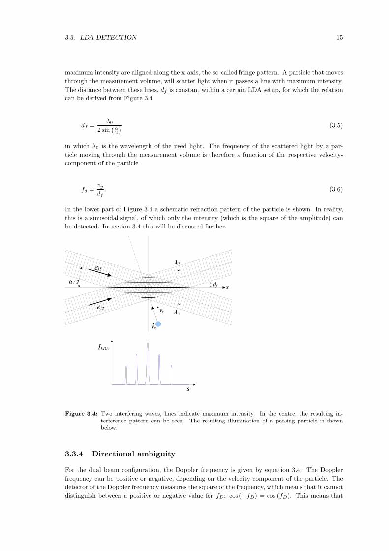
3.3. LDA DETECTION 15
maximum intensity are aligned along the x-axis, the so-called fringe pattern. A particle that moves
through the measurement volume, will scatter light when it passes a line with maximum intensity.
The distance between these lines, df is constant within a certain LDA setup, for which the relation
can be derived from Figure 3.4
df =λ0
2 sin(
α2
) (3.5)
in which λ0 is the wavelength of the used light. The frequency of the scattered light by a par-
ticle moving through the measurement volume is therefore a function of the respective velocity-
component of the particle
fd =vy
df. (3.6)
In the lower part of Figure 3.4 a schematic refraction pattern of the particle is shown. In reality,
this is a sinusoidal signal, of which only the intensity (which is the square of the amplitude) can
be detected. In section 3.4 this will be discussed further.
Figure 3.4: Two interfering waves, lines indicate maximum intensity. In the centre, the resulting in-terference pattern can be seen. The resulting illumination of a passing particle is shownbelow.
3.3.4 Directional ambiguity
For the dual beam configuration, the Doppler frequency is given by equation 3.4. The Doppler
frequency can be positive or negative, depending on the velocity component of the particle. The
detector of the Doppler frequency measures the square of the frequency, which means that it cannot
distinguish between a positive or negative value for fD: cos (−fD) = cos (fD). This means that

16 CHAPTER 3. LASER DOPPLER ANEMOMETRY
for ‘plane’ LDA it is not possible to detect the direction of the movement of a particle.
A way to solve for the above mentioned ambiguity is by frequency shifting. A frequency shift
of constant value fs of the order of the Doppler frequency is applied to one of the two beams in the
dual beam setup (Figure 3.3(b). This shift can be made by an acousto-optic Bragg cell. Assuming
that fs ≪ fD, the relationship between the Doppler frequency and the particle velocity becomes
fD = fs +2vy sin
(α2
)
λ0. (3.7)
This effect is illustrated in Figure 3.5. As long as fs is chosen to be larger than the highest |fD|for the unshifted beams, the frequency |fD| will be uniquely corresponding to a velocity value and
a direction in the flow, as a consequence removing the directional ambiguity.
Figure 3.5: Visualisation of the frequency shifting. Within the determined range, each |fD| correspondsto a single velocity v.
3.3.5 Measurement volume
The measurement volume is created at the point of intersection of two laser beams. Due to a gaus-
sian distribution of the intensity inside a laser beam, the measurement volume itself is elipsoidially
shaped, with a geometry as given in Figure 3.6. According to Adrian [15], the dimensions of the
measurement volume in respective x-, y- and z-direction can be expressed as:
dm =de−2
cos (κ)(3.8)
lm =de−2
sin (κ)(3.9)
hm = de−2 (3.10)
with de−2 the diameter of the focused laser beam, which can be expressed as
de−2 ≃ 4fλm
πDe−2
(3.11)

3.3. LDA DETECTION 17
where λm is the wavelength inside the medium, f the focal length of the lens and De−2 is the
diameter of the incoming laser beam. From equation 3.11 it can be seen that for small measurement
volumes, either large incoming beam diameters are required or short focal lengths.
Figure 3.6: Geometry of the measurement volume.
3.3.6 Particles
With LDA, the velocity of the tracer particles is determined, not of the fluid itself. Therefore,
choice of the particles is very important for a correct representation of the fluid flow.
Various requirements for the particles need to be fullfilled:
• The particles must be small and light enough to follow the smallest vortices in the flow. This
smallest scale is in the order of the Kolmogorov micro scale.
• Presence of the particles should not influence the fluid, both dynamically and chemically. A
chemical pollutant, like oxides, might distort the optical accessibility of the flow.
• Particles should have a high reflectivity for the incident light.
As a practical implementation of the preceding requirements, hollow glass spheres seem to be a
very suitbale choice according to the needs, and they are cheap as well.
The ability of the particles to follow the flow, is mostly dependent on their density difference
with the liquid and size. Particle motion is determined by drag, buoyancy and gravity forces and
inertia. The lagrangian motion of a rigid, spherical particle in a viscous flow can be described
by the Basset-Bousinesq-Oseen (BBO) equation [14]. A simplified version of this equation can be
used for seeding particles
π
6d3ρp
dvp
dt= −3πµd(vp − vf ) (3.12)
where the gravity and buoyancy forces are neglected. The left-hand side of 3.12 indicates the
acceleration force, the right-hand sight represents stokes’ drag.
Another way to describe the ability of the particles to follow the flow, is by expressing their
motion in Fourier components. As long as their maximum frequency is higher than the fluids
highest frequency, the particles can track the smallest flow structures. The flow frequency is given

18 CHAPTER 3. LASER DOPPLER ANEMOMETRY
by ω = 2πfturb. By using the substitution proposed by Tummers [14], vf = eiωt and vp = η(ω)eiωt
the amplitude ratio, |η|, can be expressed as
|η(ω)| =Ω√
Ω2 + ω2where Ω =
18ν
σrd2p
, (3.13)
with σr the density ratio ρp/ρf . The amplitude ratio is a measure of the particles sensitivity to
follow changes in fluid flow. It can be seen from equation 3.13 that for very high frequencies the
amplitude ration η becomes negligible and therefore the particles are less sensitive for the fluids
motion.
To obtain a sufficient temporal resolution to capture the smallest flow structures, at the Kol-
mogorov microscale, enough particles should cross the measurement volume. As a criterion for
the minimum sampling rate, Durst et al. [13] mentions a minimal sampling frequency of 2fturb.
Because particles are distributed randomly in the fluid, particle arrivals at the control volume are
not equally distributed in time. To ensure enough samples during moments of high velocity fluctu-
ations as well, the average particle arrival frequency should be above 2fturb to meet the minimum
condition.
3.4 Signal processing
At the surface of the photo detector, the square of the amplitude of the heterodyning frequency
is captured. This is a superposition of the pedestal and the actual burst. In the post-processing,
this pedestal needs to be removed before the actual velocity calculation can be done.
Over the years, many different post-processing mechanisms have been developed for LDA, which
have been introduced on the market by different companies. They all have different ways in esti-
mating the average particle velocity, as well as schemes for further statistics with respect to the
burst distribution. It is beyond the scope of this thesis to treat all the different methods, only the
one used during this project will be discussed in this section.
This section is split into two parts, first the processing by TSI’s Intelligent Flow Analyser (IFA)
750 will be discussed, then the filtering and statistical interpretation software, which is developed
within the Multi Scale Physics Department of Delft University of Technology.
3.4.1 Intelligent Flow Analyser
The IFA 750 is a Burst Correlator Processor, which performs an autocorrelation analysis of the
bandfiltered input signal. This input consists of the electrical output of the TSI Color Link, in
which the light bursts are sampled using a photo multiplier, a high band-pass filter removes the
pedestal, and a frequency mixer applies the selected frequency shift electronically. The IFA uses
the time delay corresponding to the first absolute minimum of the autocorrelation function to
determine the Doppler frequency.
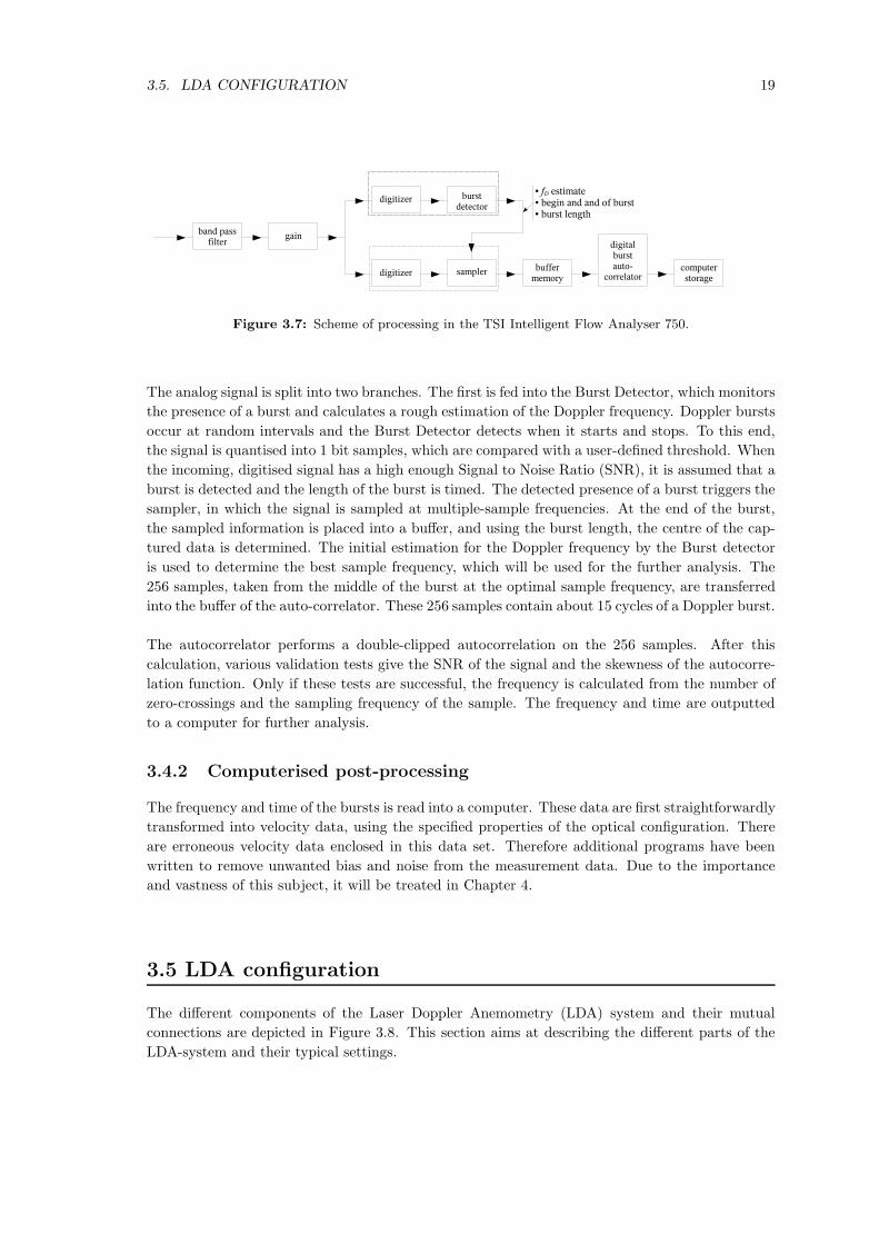
A scheme of the different operations performed inside the IFA 750 is given in Figure 3.7. The
incoming signal is initially filtered using a band-pass filter. This filter removes wide-band noise. A
fixed gain amplifier then amplifies the signal.
3.5. LDA CONFIGURATION 19
Figure 3.7: Scheme of processing in the TSI Intelligent Flow Analyser 750.
The analog signal is split into two branches. The first is fed into the Burst Detector, which monitors
the presence of a burst and calculates a rough estimation of the Doppler frequency. Doppler bursts
occur at random intervals and the Burst Detector detects when it starts and stops. To this end,
the signal is quantised into 1 bit samples, which are compared with a user-defined threshold. When
the incoming, digitised signal has a high enough Signal to Noise Ratio (SNR), it is assumed that a
burst is detected and the length of the burst is timed. The detected presence of a burst triggers the
sampler, in which the signal is sampled at multiple-sample frequencies. At the end of the burst,
the sampled information is placed into a buffer, and using the burst length, the centre of the cap-
tured data is determined. The initial estimation for the Doppler frequency by the Burst detector
is used to determine the best sample frequency, which will be used for the further analysis. The
256 samples, taken from the middle of the burst at the optimal sample frequency, are transferred
into the buffer of the auto-correlator. These 256 samples contain about 15 cycles of a Doppler burst.
The autocorrelator performs a double-clipped autocorrelation on the 256 samples. After this
calculation, various validation tests give the SNR of the signal and the skewness of the autocorre-
lation function. Only if these tests are successful, the frequency is calculated from the number of
zero-crossings and the sampling frequency of the sample. The frequency and time are outputted
to a computer for further analysis.
3.4.2 Computerised post-processing
The frequency and time of the bursts is read into a computer. These data are first straightforwardly
transformed into velocity data, using the specified properties of the optical configuration. There
are erroneous velocity data enclosed in this data set. Therefore additional programs have been
written to remove unwanted bias and noise from the measurement data. Due to the importance
and vastness of this subject, it will be treated in Chapter 4.
3.5 LDA configuration
The different components of the Laser Doppler Anemometry (LDA) system and their mutual
connections are depicted in Figure 3.8. This section aims at describing the different parts of the
LDA-system and their typical settings.

20 CHAPTER 3. LASER DOPPLER ANEMOMETRY
Figure 3.8: Scheme of different components in LDA setup
3.5.1 Laser
The laser is a Stabilite 2016 of Spectra-Physics, water cooled Ar-laser, delivering up to 4 W of
multiline Argon spectrum in the visible spectrum range (457.9 nm - 514.5 nm) with two high-power
lines at 488.0 nm (1.7 W) and 514.5 nm (1.3 W). The coherence length is about 40 mm.
3.5.2 Colorburst
The TSI Colorburst 9201 separates the laser light into different pairs of laser beams, where one
beam of each pair is shifted by the acousto-optic modulator, a Bragg cell. Three beam pairs can be
outputted: green (λ = 514.5 nm), blue (λ = 488.0 nm) and violet (λ = 476.5 nm). In the present
setup only the first two wavelengths are used. The shifting has a constant value of 40 MHz, and
is driven by a sinusoidal signal generated in the Colorlink. Each beam is equipped with an own
shutter and is coupled into a glass fibre, which guides the beam to the probe.
3.5.3 Probe
The TSI 9832 probe, with a diameter of 83 mm, contains all optical components to emit the laser
beams and collect the reflected light. It receives laser beams from the Colorburst by glass fibres
and each pair is emitted with an intermediate distance of 50 mm and the different pairs are placed
orthogonally, to measure two different velocity components simultaneously. The beams are focused
using a 132.0 mm lens.
The blue laser beams are used for the axial velocity component, because these beams deliver
a lower data-rate than the green ones and the streamwise velocity will provide relatively lower
velocity fluctuations. The high data-rate of the green beams can be used for the relatively high
fluctuations of the flow in the direction perpendicular to the streamwise direction. Figure 3.9 shows
the distribution and trajectories of the laser beam pairs in the flow setup.
The diameter of the laser beams has been determined to be 3.0 mm. The dimensions of the
measurement volume are given in Table 3.1, where the meaning of the symbols can be found in
section 3.3.5, as well as their derivation.

3.5. LDA CONFIGURATION 21
Table 3.1: Measurement volumes in water for the used setup, according to Equation 3.8.
λ dm (µm) lm (mm) hm (µm)488.0 27.6 0.205 27.3514.5 29.1 0.216 28.8
(a) Side view. (b) Front view of the probe, the blue and green spotsindicate the position where the laser beams leave theprobe.
Figure 3.9: Beams emitted from a LDA probe with respect to the flow. Blue lines indicate the 488.0 nmbeams and green indicates the 514.5 nm beams.
3.5.4 Colorlink
The TSI Colorlink 9230 is a multicolour receiver for LDA, which receives the scattered light from
the probe. The Colorlink splits this beam into the different colours and measures the intensity of
each colour separately using a photo multiplier.
The Colorlink provides a 40 MHz signal to the Colorburst to shift one beam of each pair. The
Colorlink shifts the 40 MHz shift electronically back to a user defined setting. This signal is
outputted in an analogue, electronic signal.
3.5.5 Intelligent Flow Analyser 750 and FIND software
The TSI Intelligent Flow Analyser (IFA) 750 is a burst correlator. It can take up to three input
signals, which are filtered and sampled individually. The bursts that result from the filtering
and sampling procedure are outputted towards a computer system and can be visualised on an
oscilloscope.
All settings of the IFA 750 and all outputs are managed by an accompanying computer program
called ‘Find’. The various filter, sampling settings and output format of the IFA can be set in this
program.
The procedure applied to the input in the IFA 750, is discussed in section 3.4.1. The common
settings for operation are given in section 6.2.
22 CHAPTER 3. LASER DOPPLER ANEMOMETRY
3.5.6 Traversing system
The probe is mounted on a traversing system, such that the measurement volume can reach the
complete cross-section of the test section, and also traverse along the vertical axis. These move-
ments can be controlled using a second computer system, which is coupled to the FIND software.
After finishing measurements at a certain spot, the software will automatically move the probe to
a new, pre-defined position on the measurement grid.
Due to refraction, displacement of the probe will not correspond to the displacement of the mea-
surement volume. The refractive index of water, nw is higher than that of air na, changing the angle
of the incident beam in the measurement volume. The correction factor between the movements
of the probe and the movements of the measurement volume, are given by:
CL =tan(α)
tan(
arcsin(
na
nwsin(α)
)) (3.14)
where α is given by arctan(
D/2L
)
, with D the distance between the beams and L the focal length
of the lens.
Other refractive changes might be occurring, but since these are much smaller and more difficult
to correct for, for the time being they will be neglected.
3.5.7 Seeding particles
The seeding particles that are used have a diameter of 8 - 12 µm, a density of 1.05 - 1.15 kg/m3
and a refractive index of 1.5.
The quantity of seeding added to the water, was adjusted such that LDA bursts did not over-
lap. The maximum amount of seeding during the experiment did not exceed 1 10−4% volume.
Because of this very small amount, it is therefore assumed that the fluid properties remained
unchanged by the particles.
Summary
• Laser Doppler Anemometry (LDA) is an optical method for fluid velocity measurements with
a high spatial resolution, using the Doppler shift of light caused by moving particles.
• The velocity of individual particles is determined
• The size of the measurement volume is 0.21 mm in the line of the probe and 0.03 mm
perpendicular to this line.

CHAPTER 4
Post-processing
The data acquired from the LDA signal processor (the IFA 750, see Chapter 3), consists of a time-
series of velocities, corresponding to the tracer particles flowing through the measurement volume.
Various steps need to be performed, in order to transform this into reliable turbulence statistics.
This chapter describes the post-processing software used for this thesis work. The programs are
written in Fortran programs kindly provided provided by R. Belt [7] and slightly modified during
this project.
The characteristics of the particles’ velocity data form the basis of the post-processing, and are
described in section 4.1. The quantities that need to be derived from this data are given in section
4.2 and the processing that has been done is explained in section 4.3.
4.1 Raw data
This section describes the incoming LDA signal, that is retrieved from the the IFA 750 burst
correlator. The data that is outputted by this correlator, consists of a table containing the time a
particle is detected, and its corresponding velocity, as is calculated on basis of the fringe spacing
in the corresponding measurement volume. All further data treatment inside the software of the
IFA is disabled, and performed by independent software which is described in section 4.3.
4.1.1 Particle distribution
Interarrival time distribution
The particles in the fluid have a random distribution throughout the fluid, that results in a random
passage of the tracer particles through the measurement volume. For LDA, this interarrival particle
distribution can be described as a Poisson distribution [14], for which the probability density
function of the interarrival times (∆t) is given by:
p (∆t) = λe−λ∆t (4.1)
where λ is the mean number of samples per unit of time, or the mean data-rate.
23
24 CHAPTER 4. POST-PROCESSING
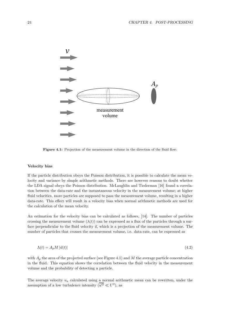
Figure 4.1: Projection of the measurement volume in the direction of the fluid flow.
Velocity bias
If the particle distribution obeys the Poisson distribution, it is possible to calculate the mean ve-
locity and variance by simple arithmetic methods. There are however reasons to doubt whetter
the LDA signal obeys the Poisson distribution. McLaughlin and Tiederman [16] found a correla-
tion between the data-rate and the instantaneous velocity in the measurement volume; at higher
fluid velocities, more particles are supposed to pass the measurement volume, resulting in a higher
data-rate. This effect will result in a velocity bias when normal arithmetic methods are used for
the calculation of the mean velocity.
An estimation for the velocity bias can be calculated as follows, [14]. The number of particles
crossing the measurement volume (λ(t)) can be expressed as a flux of the particles through a sur-
face perpendicular to the fluid velocity ~u, which is a projection of the measurement volume. The
number of particles that crosses the measurement volume, i.e. data-rate, can be expressed as
Λ(t) = ApM |~u(t)| (4.2)
with Ap the area of the projected surface (see Figure 4.1) and M the average particle concentration
in the fluid. This equation shows the correlation between the fluid velocity in the measurement
volume and the probability of detecting a particle.
The average velocity ua calculated using a normal arithmetic mean can be rewritten, under the
assumption of a low turbulence intensity (u′2 ≪ U2), as

4.1. RAW DATA 25
ua =u(t)Λ(t)
Λ(t)=
|u(t)|u(t)
u(t)≈ u(t)2
u(t)= U +
u′2
U. (4.3)
A higher turbulence intensity, increases the velocity bias. It is possible to correct for the bias effect
in the post-processing. This will be treated in section 4.3.4.
Altough the first publications on the velocity bias are more than 30 years old, there is still a
debate on the best correction method, as well as on the existence of the velocity bias in general. In
a series of articles, of which Tummers [14] states that the velocity bias disappears at low data-rates.
This was contrary to Tummers [14] own findings.
Multiple particles
Since the distribution of particles is random, it can occur that two particles are present in the
measurement volume within a negligible interval. The minimum particle size of 8 µm is smaller
than the height of the measurement volume, about 30 µm, allowing multiple particles to reside in
the measurement volume. The two overlapping bursts can interfere with each other and lead to a
misinterpretation of the velocity.
Another possible error might occur when the detector sees the burst of one particle as two separate
bursts. In the calculation of the mean velocity and variance, too much weight will be given to this
particle. A solution for this is given in section 4.3.2.
4.1.2 Detector characteristics
Dead time of processor
As long as the processor is occupied with a burst, it cannot collect and process the data retrieved
from a new burst. The time between the end of a burst and the availability of detecting a new
burst is known as the dead time of the processor. If two particles have a too short interarrival
time, the particle arriving later will not be detected. This poses a limitation on the shortest time
scale that can be measured using the LDA setup.
No coincidence
For the determination of Reynolds stresses, the instantaneous velocities in two directions need to
be correlated. A particle moving through the measurement volume does not need to be detected
at the same time for both colours (and directions). It might be the case that the measurement
volume for each colour does not overlap exactly due to refraction issues, resulting in a difference
in time of detection, or a burst might be filtered away for one of each direction. To resolve this, a
criterion needs to be applied to decide whether or not two bursts coincide.
Other noise
An amount of specific seeding is added to the water, such that the seeding particles follow the
flow and all of its small swirls, see section 3.3.6. Some impurities in the seeding material or in
the fluid itself can also generate bursts. These particles can be too large and heavy, resulting in
more inertia of the particle and they do not have the ability of following all small flow structures.

26 CHAPTER 4. POST-PROCESSING
Another difference might be their density, resulting in a buoyant force on the particles and an error
in their velocity.
The burst detector continuously monitors the signal from the photomultiplier, to detect whether
a burst is seen, see section 3.5. If a burst is detected, the processor starts sampling and processing
the burst. Due to some noise in the photomultiplier output, or an electronic noise, some bursts can
be sampled that are not a real burst, but just noise. Of course, their velocity will not correspond
to the instantaneous fluid velocity.
4.2 Calculated velocity information
Laser Doppler Anemometry is used to gain insight in fluid flows. This section describes the different
quantities which could be calculated in the post-processing.
4.2.1 Velocity profile
The most commonly used type of information about a flow, is a velocity profile of the mean
velocity at each point. It unveils the secondary flow pattern and can be used to estimate molecular
transport throughout the fluid. The addition of the variance in the velocity of the particles, gives
information on the spread of the fluid velocity and may indicate alternating structures.
As explained in section 4.1, there are some sources of error in the signal. These should be removed
in the different post-processing steps.
4.2.2 Autocorrelation function
The autocorrelation function (ACF) of the velocity is a measure for the dependence of the velocity
on the velocity at the same point at a time τ before that moment. The ACF is given by
Ruu(τ) =u′(t)u′(t + τ)
u′2(τ)(4.4)
where u′ is the difference between the instantaneous and mean velocity at a certain point.
The ACF for τ = 0 can be used to calculate the Reynolds-stress term −ρu′
iu′
i. The smallest time
scales in the flow are also indicated by the ACF, a rapid decrease of the acf to 0 is caused by a
small Taylor time scale. An estimate for the Taylor time scale is given by Absil [17]:
T 2λ =
−2(
∂2ru′u′ (τ)∂τ2
)
τ=0
, (4.5)
which is the curvature of the acf at τ = 0.
4.2.3 Stresses
The Reynolds-stresses u′u′, u′v′ and v′v′ are very interesting with respect to the transport of
momentum throughout the fluid flow and as estimate of the turbulence.

4.3. DATA FILTERING AND CORRECTION 27
The stresses can be calculated using the autocorrelation function as described above, or by using
a direct correlation between all velocity samples.
4.3 Data filtering and correction
This section describes the various operations performed on the raw data by using the Fortran 95
program set, in the order as the different steps are applied to the data.
4.3.1 Clipping
The process of clipping removes the velocity samples having a difference of more than ±n times
the standard deviation (σ) compared to the mean velocity. It is likely that these samples are
taken from non-appropriate particles that reflect light, or are captured when no particle passed
the measurement volume.
The value of n is chosen to be 5 during this research.
4.3.2 Multiple Validation
As described in section 4.1.1, it can be possible that one particle is seen as two different bursts.
These bursts are characterised by a very short interarrival time. A solution to this problem is
to increase the dead time of the processor artificially, i.e., by not taking into account bursts that
follow within a time tdead of another burst. This dead time is a user defined value and needs not
to be longer than the transit time of particles through the measurement volume.
This strategy removes also two different particles that are very close to each other, where it might
happen that their bursts overlap or distort each other.
4.3.3 Coincidence window
As explained in section 4.1.2, the two bursts (for the two directions) from one particle do not
need to occur at exactly the same time, or one of the both velocity samples might be missing.
The single velocity samples, as well as those with a certain time lag need to be removed to do a
calculation of the Reynolds-stresses. For this calculation, it is assumed that the bursts for each
direction originate at the same time and position.
To allow small deviations, the technique of a coincidence window is applied. The difference in
particle detection for both the measurement volume (each color) are checked against a predefined
threshold: |tchannel 1 − tchannel 2| < τc.
The value for τc must be smaller than the particle’s transit time through the measurement volume,
which is in practice an order smaller than the average interarrival time. In general, a smaller value
for τc improves the correlation, but lowers the data-rate.
4.3.4 Velocity bias
The origin of the velocity bias is discussed in section 4.1.2. This section describes the methods to
correct for the velocity bias.
Two different approaches can be applied; (i) resampling of the irregular signal and (ii) assigning

28 CHAPTER 4. POST-PROCESSING
weights to velocity samples to compensate for the irregular sampling. Both methods will be
discussed in the following paragraphs.
Sampling techniques
The velocity bias is caused by an irregular sampling of the velocity data. The different sampling
techniques deals with this by resampling the signal on a regular interval. Calculating the mean
velocity based on these results in an arithmetic way will provide an unbiased result.
The various sampling techniques are treated by Tummers [14] with relevant references to literature.
The data density, in combination with the smallest time scale of the fluid (the Taylor microscale)
plays an important role, for these resampling schemes, since they should have a high enough
resolution in time. Three different resampling techniques are:
• controlled processor: The signal is divided in equally long time intervals. Inside each time
interval, the first sample is used for further processing.
• saturated processor: The processor is inhibitted after taking each sample for a time ts.
This results in a nearly equidistant time series.
• sample-and-hold processor: A continuous signal is made by holding the last velocity,
until a new one is taken. Based on that, the signal can be reconstructed by a higher-order
polynomial.
Altough resampling is very robust in generating an unbiased timeseries, there are some draw-
backs; the controlled processor and saturated processor tend to decrease the data-rate significantly,
whereas the sample-and-hold processor requires a polynomial fitting of the data, which cannot be
easily implemented.
Weighting factors
The method of weighting factors approaches the correction for bias by a change in the calculation
of two statistical values, the mean velocity and the velocity variance. The numerical importance
of various data points is rewarded using the weighing factor, ω, of a point, leading to the following
statistical quantities:
u =
∑Ni=1 uiωi∑N
i=1 ωi
u′2 =
∑Ni=1 u′2
i ωi∑N
i=1 ωi
(4.6)
with u the mean velocity, u′2 the variance and i the ith velocity sample. For ω = 1, the calculations
transform to the normal, arithmetic, versions. The summation runs over all velocity samples. For
the weighing factors, the following schemes are known:
• inverse velocity: Equation 4.2 shows the correlation between the data-rate and the velocity
flux, for flows with a constant particle density M . The inverse of the volume flux can therefore
be used as a weighting factor, the so-called inverse-velocity weighting:
ω =1
Ap|~v|=
1
Ap
√u2 + v2 + w2
. (4.7)
This formula is known as 3D inverse-velocity weighting, since all three velocity components
are used. For this research, just two velocity components are available, resulting in the 2D
inverse-velocity weighting:

4.3. DATA FILTERING AND CORRECTION 29
ω =1√
u2 + v2. (4.8)
Because the third component is not taken into account in 4.8, the ω is always too high.
Nakayama [18] worked around this problem, by estimating a value for the third velocity
component. For a two-dimensional flow, with w = 0, the weighting factor reads
ω =1
√
u2 + v2 +(
dl
)2w′2
, (4.9)
with dl the length (l) to width (d) ratio of the measurement volume. w′2 can be approximated
by different models, using the two known velocity components. The weighting factor in
equation 4.9 is known as 2D+ weighting.
• transit-time: The volume flux as used in the inverse velocity weighting can be considered
to be equivalent to weighting with the mean time particles need to transit the measurement
volume, for a given velocity vector:
tre =1
Ap
∫
Ap
tr d Ap, (4.10)
with tr the time during which each individual particle is inside the measurement volume.
Practical issues for this correction method include the difficulty of measuring the transit
time.
• interarrival-time: The time between subsequent velocity samples is used as weighting
factor:
ω = ∆ti ≡ ti+1 − ti (4.11)
This correction takes the unequal particle distribution into account and provides in that sense
an improvement over the inverse velocity factor scheme. For short, this method is indicated
as IT weighing.
The result of the IT weighing is only unbiased for high data-rates, as a criterion Edwards
et al. [19] give
νλt > 10, (4.12)
with ν the data-rate and λt the Taylor time scale.
For the current research, the 2D+-weighting scheme is used for the velocity bias elimination,
because the data-rate criterion for the IT-weighting is not reached for this flow.
4.3.5 Correlation calculation
The autocorrelation function (ACF) was introduced in section 4.2.2. Because LDA data is ran-
domly sampled, it is not possible to use default methods to calculate the spectral density. Mayo
et al. [20] were the first to introduce a solution to this problem, with the so-called slotting tech-
nique, that will be treated below. This slotting technique was not able to give reliable estimates
for high-frequency ranges. Various improvements were proposed to solve this, they are treated in
the second part of this section.
A different scheme to calculate the ACF was introduced by Nobach et al. [21], the refined recon-
struction. This estimation is not used for this research, since the (improved) slotting technique
was proven by Muller et al. [22] to be slightly superior to the refined reconstruction technique.

30 CHAPTER 4. POST-PROCESSING
Slotting technique
The slotting technique is a discrete way of calculating an acf. The time lag axis, ∆τ is divided
into bins or “slots”, which are not necessarily equally large. The product of the velocities that fall
within a certain bin is added to the bin’s sum. Each product is an estimation of the ACF for that
value of the time lag. Finally, each bin is divided by the number of products inside, resulting in an
averaged out estimation for the acf for each ∆τ . A formal representation of this process is given
by Benedict et al. [23]:
Ru′u′(k∆τ) =
∑Ni=1
∑Nj=1 uiujbk(tj − ti)
∑Ni=1
∑Nj=1 bk(tj − ti)
, (4.13)
with bk(tj − ti) =
1 for∣∣∣(tj−ti
∆τ − k∣∣∣ < 1
2
0 otherwise(4.14)
with the two different velocity samples ui = u(ti) and uj = u(tj).
Due to dead time present in the hardware, and the rejection of particles with a very short interar-
rival time, the estimate of the ACF for very small τ is based on just a few velocity products. This
makes the correlation very unreliable for small time lags. To work around this problem, different
improvements of the slotting technique have been made, which are treated in the next section.
Improvements of slotting technique
The different improvements of the slotting technique are discussed in this section, in chronological
order of their publication. The different corrections can be implemented in the same algorithm.
• Local normalisation: first published by Tummers and Passchier [24]. Due to the sta-
tionarity of the process, (u(t)2u(t + τ)2)1/2 = u2, the autocovariance can be rescaled by a
discretised version of (u(t)2u(t + τ)2)1/2, which is
Jk =
(
bk
∑Ni=1 u2
i
∑Nj=1 u2
j
)1/2
∑Ni=1
∑Nj=1 bk(tj − ti)
(4.15)
where bk is the same in in equation 4.13. Jk is an estimate for the variance of each slot
independently. The autocorrelation function ρk then follows from:
ρk =Rk
Jk
(4.16)
• Fuzzy Slotting: Introduced by Nobach et al. [25], the fuzzy slotting techniques changes the
weighting function bk to
bk(tj − ti) =
1 −∣∣∣(tj−ti
∆τ − k∣∣∣ for
∣∣∣(tj−ti
∆τ − k∣∣∣ < 1
0 otherwise. (4.17)
The weighting functions make that the slots overlap with adjacent slots, see Figure 4.2. The
non-sharp edges of the slots reduce the quantisation noise, and contribute to a lower variance
of the correlation estimate.

4.3. DATA FILTERING AND CORRECTION 31
Figure 4.2: Fuzzy slotting weighting scheme, based on Benedict et al. [23].
• Weighting algorithms: This technique (Nobach [26]) uses the weighting factors that are
used for the calculation of the mean velocity and variance as described in section 4.3.4.
The velocity ui is replaced by wiui (wi is the weighting factor). Different schemes can
be applied, like arrival-time weighting or forward-backward arrival time weighting. This
weighting algorithm compensates for the unequal sampling, which increases the performance
of the processor.
• Local time estimation: Nobach [27] introduced this scheme, because the velocity samples
in a certain bin do not need to be distributed equally over the bin. The use of an average
time lag τk instead of the predefined value τk = k ∗ ∆τ , improves the estimated correlation
function Rk, because it assigns a better time lag to each slot.
The averaged time lag per bin is given by:
τk =
∑N−1i=1
∑Nj=i+1(tj − ti)wiwjbk(tj − ti)
∑N−1i=1
∑Nj=i+1 wiwjbk(tj − ti)
. (4.18)
This equation presents the average time lag, with also the fuzzy slotting technique and
weighting scheme taken into consideration.
The fuzzy slotting technique with local normalisation as described above is used for the post-
processing of the data in this project.
4.3.6 Model-based fitting of the correlation function
The correlation function for very small time lags and τ = 0 are of great interest for the determi-
nation of the Reynolds-stresses and for estimating the Taylor time scale of the flow. Especially in
bins with the smallest time lag, the number of correlation estimators is very low, which results in
an insufficient estimate of the correlation function for small time lags.
Based on limited number of correlation estimators that is available for the small time, the corre-
lation function can be modelled, according to van Maanen and Oldenziel [28]. Since only really

32 CHAPTER 4. POST-PROCESSING
small time lags need to be modelled, these models do not necessarily need to contain periodic
components. There are three different models proposed in literature:
• Van Maanen and Tummers [23, ref 1996] use a gaussian function around τ = 0 top estimate
a fit to the correlation function:
ru′u′(k∆τ) = a e−b (k∆τ)c
(4.19)
where a, b and c are scaling variables.
• Nobach [27] suggests a parabolic function:
ru′u′(k∆τ) = a − b(k∆τ)c (4.20)
• As an alternative, Nobach [27] proposes a different kind of function:
ru′u′(k∆τ) = a(b ec k∆τ − c eb k∆τ
)(4.21)
Summary
• The LDA data contains various error sources like irregular interarrival times, multiple vali-
dation and a velocity bias.
• Various techniques are presented to correct for the different sources of errors.
• The slotting technique is introduced to calculate the correlation of an LDA signal.
CHAPTER 5
Refractive Index Matching
This chapter aims at giving more information on the refractive index matching of Fluorinated
Ethylene Propylene (FEP) to that of the fluid used in the experiment: water.
The reason for the refractive index matching, different methods and the behaviour of the method
chosen for this research, are treated in subsequent order in this chapter.
5.1 Motivation
Optical measurement techniques are commonly used and are non-intrusive in nature. An important
condition that needs to be fullfilled for using these techniques, like LDA, is to optically access the
region of interest in the fluid. Difference in the refractive indeces between the fluid, solid walls and
environment can change the position of the measurement volume from its expected value, due to
refraction at the different surfaces. This refraction is described by Snell’s law:
n1 sin θ1 = n2 sin θ2 (5.1)
here n is the refractive index of the material, θ is the angle of incidence with the normal and 1 and
2 indicate two different materials. The use of flat surfaces gives refractions that are predictable,
but other geometries, especially one with curved surfaces, are tremendously difficult to compensate
for.
There are two solutions to reduce the refraction by the solid walls surrounding the fluid flow: (i)
reduce the thickness of the wall or (ii) make the refractive indices n1 and n2 as equal as possible.
The first (i) method works since in the limit of an infinitely thin wall, no refraction will occur. This
chapter focuses on the second method: the matching of refractive indices, because it allows flow
field measurements in more difficult shapes like a tube bundle geometry, using optical techniques.
5.2 Types of refractive index matching
In general, two different methods of refractive index matching can be recognised; (i) the fluid can
be matched to the solid material, or (ii) the solid can be matched to the liquid.
33

34 CHAPTER 5. REFRACTIVE INDEX MATCHING
Figure 5.1: Trajectory of a laser beam through the walls of a FEP cylinder. Due to refraction, the beamwill be deviated by a small angle when leaving the cylinder, this angle is indicated.
The first option is usually based on commonly used solids, like glass and poly methyl methacrylate
(PMMA), with a typical refractive index of 1.52 and 1.49 respectively, [29]. There are various
possibilities for matching fluids to these solid materials, like dissolved zinc salts or benzyl alcohols.
Although the liquids are completely different, they have some major disadvantages in common.
One should think of a high price, toxicity and a strong temperature dependence of the refractive
index.
For the match of the solid to the liquid, the use of water (n ≈ 1.38) is highly preferred, since it is
cheap, widely available, non-toxic and has well known properties. There are very little transparent
materials known that have a matching refractive index to water. Fluorinated Propylene Ethylene
(FEP) is one such potential candidate with a refractive index in literature of 1.338. Therefore, in
this project FEP as a refractive index matching material with water is studied.
5.3 FEP
5.3.1 Optical properties
For a practical use of FEP as a refractive index matching material, the optical properties are very
important. Two important properties are studied: the refractive index and the transmittance of
the light.
Refractive index
Experimental determination of the refractive index of FEP has been carried out for the two colours
of the laser beams applied using a cylindrical geometry. When the light beam enters the cylinder
at a different position other then the centre, it will be refracted by the difference in the refractive
index of the cylinder and the surrounding water, see Figure 5.1. The size of the resulting angle (γ
in Figure 5.1) is a measure for the refractive index. The angle has been determined for 25 different
positions, each time the incident beam was parallel to the axis through the centre of the cylinder.
The expected angle of deviation has been fitted to the experimental results, with the refractive
index of FEP as a fitting parameter. For the surrounding water at 18 C, the literature value of
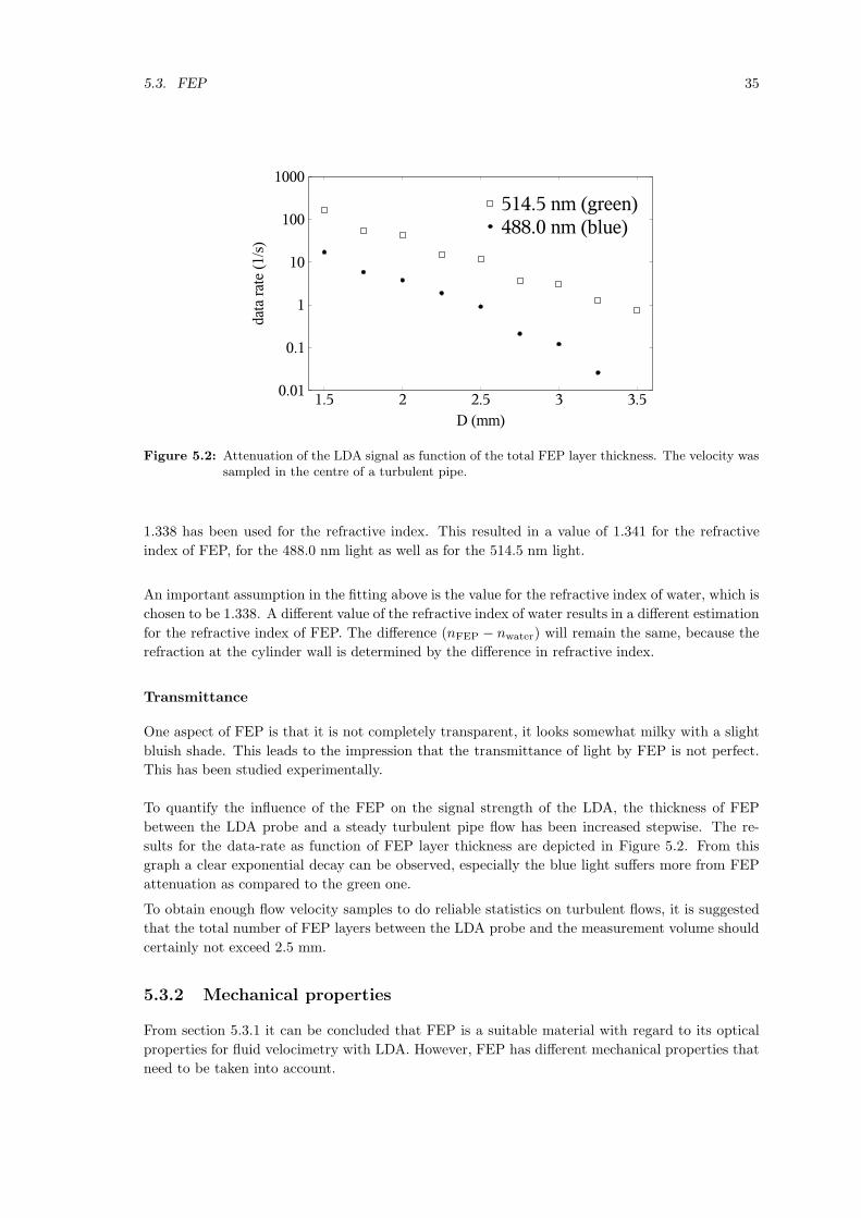
5.3. FEP 35
Figure 5.2: Attenuation of the LDA signal as function of the total FEP layer thickness. The velocity wassampled in the centre of a turbulent pipe.
1.338 has been used for the refractive index. This resulted in a value of 1.341 for the refractive
index of FEP, for the 488.0 nm light as well as for the 514.5 nm light.
An important assumption in the fitting above is the value for the refractive index of water, which is
chosen to be 1.338. A different value of the refractive index of water results in a different estimation
for the refractive index of FEP. The difference (nFEP − nwater) will remain the same, because the
refraction at the cylinder wall is determined by the difference in refractive index.
Transmittance
One aspect of FEP is that it is not completely transparent, it looks somewhat milky with a slight
bluish shade. This leads to the impression that the transmittance of light by FEP is not perfect.
This has been studied experimentally.
To quantify the influence of the FEP on the signal strength of the LDA, the thickness of FEP
between the LDA probe and a steady turbulent pipe flow has been increased stepwise. The re-
sults for the data-rate as function of FEP layer thickness are depicted in Figure 5.2. From this
graph a clear exponential decay can be observed, especially the blue light suffers more from FEP
attenuation as compared to the green one.
To obtain enough flow velocity samples to do reliable statistics on turbulent flows, it is suggested
that the total number of FEP layers between the LDA probe and the measurement volume should
certainly not exceed 2.5 mm.
5.3.2 Mechanical properties
From section 5.3.1 it can be concluded that FEP is a suitable material with regard to its optical
properties for fluid velocimetry with LDA. However, FEP has different mechanical properties that
need to be taken into account.

36 CHAPTER 5. REFRACTIVE INDEX MATCHING
FEP is chemically comparable to poly tetra fluoro ethylene (PTFE) also known as teflon. Just like
teflon, FEP has a very low friction coefficient, and almost no material can be glued to FEP. This
property imposes a difficulty in connecting the FEP to other parts in the flow setup.
FEP is a very flexible material and retains it flexibility in a temperature range of -200C to +200C.
To keep the FEP in the desired shape, precautions need to be taken, like providing additional sup-
ports.
More details on the attachment and shaping of the FEP can be found in Appendix C.
5.4 Remaining errors
Since the match in refractive index between FEP and water is not perfect, there remains some
refraction. This refraction is most noticeable at places where the angle of incidence is not fully
perpendicular, like near the edges of cylinders. This section quantifies the error in the position of
the measurement volume due to refraction in a cylinder.
The beams emitted from the LDA probe are refracted by the curved surface of the cylinder.
Here, the blue beams are taken to measure the streamwise velocity, the green beams the horizontal
velocity, as in Figure 3.9. The angle of incidence with the FEP wall of the green beams therefore
differs from that of the blue beams. The shift in position of the measurement position of the two
colours is therefore not the same. Figure 5.3 shows this effect strongly exaggerated. The expected
measurement position, is the hypothetical case where no refraction would occur.
The effects of the diffraction have been calculated based on the refractive indices retrieved in
the previous section: 1.341 for FEP and 1.338 for water. The resulting difference between the
calculated position of the measurement volume, and the expected position, are depicted in Figure
5.4, for the blue and green beams separately and for each with the two respective directions, as
declared in Figure 5.3.
From Figure 5.4 it becomes clear that the errors in position become significant when approaching
the wall very close (<1 mm). It is possible to correct for these errors, as long as one velocity
component is required. The use of the correlation between both velocity components may not
be possible due to the fact that the measurement volumes for both components do not overlap
anymore.
Summary
• The used refractive index match is adjusting the transparent solid refractive index to that of
water. This is done using FEP.
• FEPs refractive index 1.341 for light with λ ≈ 5 ·10−7m is in the order of the refractive index
for water: 1.338.
• A strong absorption of light and difficult constructive properties can limit the use of FEP.
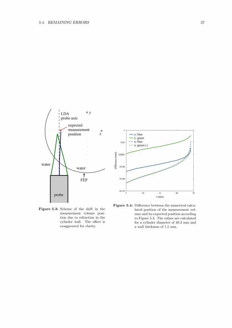
5.4. REMAINING ERRORS 37
Figure 5.3: Scheme of the shift in themeasurement volume posi-tion due to refraction in thecylinder wall. The effect isexaggerated for clarity.
Figure 5.4: Difference between the numerical calcu-lated position of the measurement vol-ume and its expected position accordingto Figure 5.3. The values are calculatedfor a cylinder diameter of 48.3 mm anda wall thickness of 1.5 mm.

38
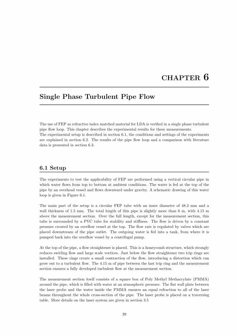
CHAPTER 6
Single Phase Turbulent Pipe Flow
The use of FEP as refractive index matched material for LDA is verified in a single phase turbulent
pipe flow loop. This chapter describes the experimental results for these measurements.
The experimental setup is described in section 6.1, the conditions and settings of the experiments
are explained in section 6.2. The results of the pipe flow loop and a comparison with literature
data is presented in section 6.3.
6.1 Setup
The experiments to test the applicability of FEP are performed using a vertical circular pipe in
which water flows from top to bottom at ambient conditions. The water is fed at the top of the
pipe by an overhead vessel and flows downward under gravity. A schematic drawing of this water
loop is given in Figure 6.1.
The main part of the setup is a circular FEP tube with an inner diameter of 48.3 mm and a
wall thickness of 1.5 mm. The total length of this pipe is slightly more than 6 m, with 4.15 m
above the measurement section. Over the full length, except for the measurement section, this
tube is surrounded by a PVC tube for stability and stiffness. The flow is driven by a constant
pressure created by an overflow vessel at the top. The flow rate is regulated by valves which are
placed downstream of the pipe outlet. The outgoing water is fed into a tank, from where it is
pumped back into the overflow vessel by a centrifugal pump.
At the top of the pipe, a flow straightener is placed. This is a honeycomb structure, which strongly
reduces swirling flow and large scale vortices. Just below the flow straightener two trip rings are
installed. These rings create a small contraction of the flow, introducing a distortion which can
grow out to a turbulent flow. The 4.15 m of pipe between the last trip ring and the measurement
section ensures a fully developed turbulent flow at the measurement section.
The measurement section itself consists of a square box of Poly Methyl Methacrylate (PMMA)
around the pipe, which is filled with water at an atmospheric pressure. The flat wall plate between
the laser probe and the water inside the PMMA ensures an equal refraction to all of the laser
beams throughout the whole cross-section of the pipe. The laser probe is placed on a traversing
table. More details on the laser system are given in section 3.5
39
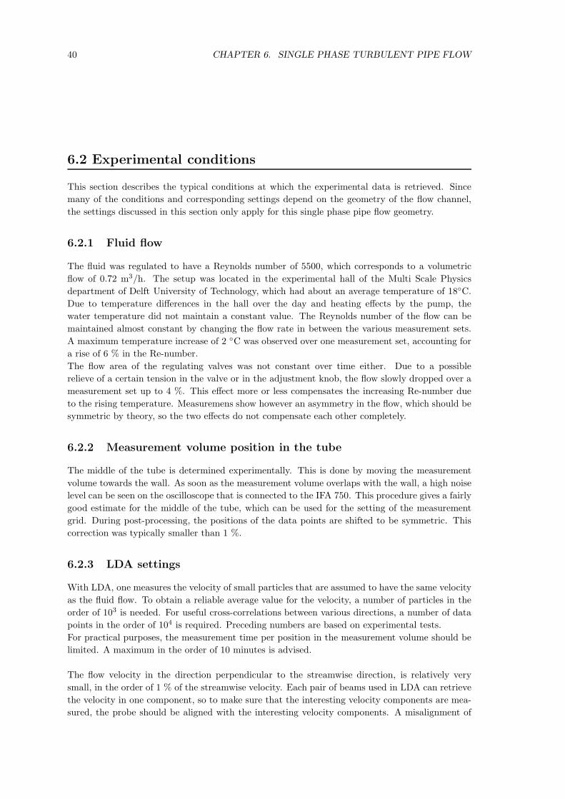
40 CHAPTER 6. SINGLE PHASE TURBULENT PIPE FLOW
6.2 Experimental conditions
This section describes the typical conditions at which the experimental data is retrieved. Since
many of the conditions and corresponding settings depend on the geometry of the flow channel,
the settings discussed in this section only apply for this single phase pipe flow geometry.
6.2.1 Fluid flow
The fluid was regulated to have a Reynolds number of 5500, which corresponds to a volumetric
flow of 0.72 m3/h. The setup was located in the experimental hall of the Multi Scale Physics
department of Delft University of Technology, which had about an average temperature of 18C.
Due to temperature differences in the hall over the day and heating effects by the pump, the
water temperature did not maintain a constant value. The Reynolds number of the flow can be
maintained almost constant by changing the flow rate in between the various measurement sets.
A maximum temperature increase of 2 C was observed over one measurement set, accounting for
a rise of 6 % in the Re-number.
The flow area of the regulating valves was not constant over time either. Due to a possible
relieve of a certain tension in the valve or in the adjustment knob, the flow slowly dropped over a
measurement set up to 4 %. This effect more or less compensates the increasing Re-number due
to the rising temperature. Measuremens show however an asymmetry in the flow, which should be
symmetric by theory, so the two effects do not compensate each other completely.
6.2.2 Measurement volume position in the tube
The middle of the tube is determined experimentally. This is done by moving the measurement
volume towards the wall. As soon as the measurement volume overlaps with the wall, a high noise
level can be seen on the oscilloscope that is connected to the IFA 750. This procedure gives a fairly
good estimate for the middle of the tube, which can be used for the setting of the measurement
grid. During post-processing, the positions of the data points are shifted to be symmetric. This
correction was typically smaller than 1 %.
6.2.3 LDA settings
With LDA, one measures the velocity of small particles that are assumed to have the same velocity
as the fluid flow. To obtain a reliable average value for the velocity, a number of particles in the
order of 103 is needed. For useful cross-correlations between various directions, a number of data
points in the order of 104 is required. Preceding numbers are based on experimental tests.
For practical purposes, the measurement time per position in the measurement volume should be
limited. A maximum in the order of 10 minutes is advised.
The flow velocity in the direction perpendicular to the streamwise direction, is relatively very
small, in the order of 1 % of the streamwise velocity. Each pair of beams used in LDA can retrieve
the velocity in one component, so to make sure that the interesting velocity components are mea-
sured, the probe should be aligned with the interesting velocity components. A misalignment of

6.2. EXPERIMENTAL CONDITIONS 41
Figure 6.1: Experimental flow loop for pipe flow measurements
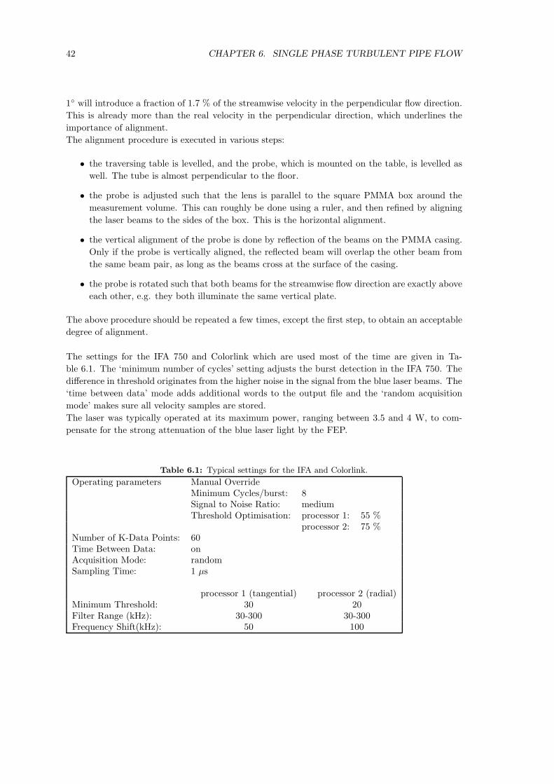
42 CHAPTER 6. SINGLE PHASE TURBULENT PIPE FLOW
1 will introduce a fraction of 1.7 % of the streamwise velocity in the perpendicular flow direction.
This is already more than the real velocity in the perpendicular direction, which underlines the
importance of alignment.
The alignment procedure is executed in various steps:
• the traversing table is levelled, and the probe, which is mounted on the table, is levelled as
well. The tube is almost perpendicular to the floor.
• the probe is adjusted such that the lens is parallel to the square PMMA box around the
measurement volume. This can roughly be done using a ruler, and then refined by aligning
the laser beams to the sides of the box. This is the horizontal alignment.
• the vertical alignment of the probe is done by reflection of the beams on the PMMA casing.
Only if the probe is vertically aligned, the reflected beam will overlap the other beam from
the same beam pair, as long as the beams cross at the surface of the casing.
• the probe is rotated such that both beams for the streamwise flow direction are exactly above
each other, e.g. they both illuminate the same vertical plate.
The above procedure should be repeated a few times, except the first step, to obtain an acceptable
degree of alignment.
The settings for the IFA 750 and Colorlink which are used most of the time are given in Ta-
ble 6.1. The ‘minimum number of cycles’ setting adjusts the burst detection in the IFA 750. The
difference in threshold originates from the higher noise in the signal from the blue laser beams. The
‘time between data’ mode adds additional words to the output file and the ‘random acquisition
mode’ makes sure all velocity samples are stored.
The laser was typically operated at its maximum power, ranging between 3.5 and 4 W, to com-
pensate for the strong attenuation of the blue laser light by the FEP.
Table 6.1: Typical settings for the IFA and Colorlink.
Operating parameters Manual OverrideMinimum Cycles/burst: 8Signal to Noise Ratio: mediumThreshold Optimisation: processor 1: 55 %
processor 2: 75 %Number of K-Data Points: 60Time Between Data: onAcquisition Mode: randomSampling Time: 1 µs
processor 1 (tangential) processor 2 (radial)Minimum Threshold: 30 20Filter Range (kHz): 30-300 30-300Frequency Shift(kHz): 50 100

6.3. RESULTS 43
6.3 Results
The results for the single phase pipe flow loop are shown in this chapter. The specification of
the setup is treated in detail in section 6.1. These experiments have been performed to obtain a
measure for the quality of FEP in fluid flow experiments.
With LDA, one obtains at a trajectory of spots velocity samples for a certain time. Choosing these
spots on a line gives a velocity profile along a line through the cylinder. There are two profiles
especially interesting, which are shown in Figure 6.2. The directions are given relative to the LDA
probe axis. One profile is parallel to the LDA probe axis and the other is perpendicular to the
LDA probe axis.
The velocity samples that are obtained contain the velocity components in the axial direction
and in the direction parallel to the perpendicular axis. The measurement spots on the perpen-
dicular axis contain therefore the axial and radial velocity components, whereas the parallel axis
contains the axial and tangential velocity components.
The size of the measurement volume is much smaller in the perpendicular direction than in the
parallel direction, as is explained in section 3.3.5. This in combination with the more interesting
radial velocity components make the perpendicular axis the preferred axis for measurements. In
ordinary tubes, the refraction in the region near the wall makes LDA very difficult with a large
error in the position of the measurement volume, see chapter 3. Results in the following sections
aim to show that FEP can solve this problem.
Figure 6.2: Alignment of measurement spots in tube with respect to the probe, and the orientation ofthe measurement volume with respect to the measurement axes.
The velocity profile of a Reynolds 5.5 · 103 flow has been obtained over the parallel and the
perpendicular axis, and these results are shown in Section 6.3.1 and 6.3.2 respectively and compared
to literature data. The differences and properties of the two profiles are discussed in section 6.3.3.
6.3.1 Parallel profile
Figure 6.3 shows the results for the velocity measurements along the parallel axis. The results
consist of three different graphs. The first, Figure 6.3(a) shows the non-dimensionalised velocities
as a function of the relative radial position. The friction velocity is determined from the near
wall axial velocity gradient, see Appendix B for details. The second graph, Figure 6.3(b) shows

44 CHAPTER 6. SINGLE PHASE TURBULENT PIPE FLOW
the same data, but as function of the non-dimensional wall distance y+, which is also covered
by Appendix B. The last graph, Figure 6.3(c), contains the root mean square (RMS) averaged
velocities for the u2z, u2
x and uzux terms. The ux term in this case is the tangential velocity and it
can be seen that ux does not correlate with the axial velocity, uz.
All graphs show reference data as far as it is available; direct numerical simulation (DNS) data
from Eggels et al. [30] and LDA data from den Toonder [31]. The line v+ = y+ is drawn as a
reference for the viscous sublayer and the function v+ = 2.78 ln y++5.5 as reference for the loglaw
layer. The value of the constant 2.78 has been determined by fitting the line to the perpendicular
velocity profile, which can be found in the next section.
6.3.2 Perpendicular profile
Figure 6.4 depicts the results that are obtained along the perpendicular axis in the pipe. It contains
three graphs: Figure 6.4(a) is the non-dimensionalised velocity profile as a function of the radial
position, Figure 6.4(b) is the non-dimensionalised velocity as a function of the non-dimensional
wall-distance y+ and Figure 6.4(c) contains the RMS averaged velocities, the so-called Reynolds
stresses. The data has been corrected for the shift in the measurement volume position which is
caused by the difference in refractive index between water and FEP.
Similar to the parallel case, reference data of Eggels et al. [30] and den Toonder [31] is shown, the
line v+ = y+ and the function v+ = 2.78 ln y+ + 5.5.
6.3.3 Discussion
As expected the results for the parallel and perpendicular direction show identical velocity profiles,
see Figures 6.3(a) and 6.4(a).The size of the measurement volume (see Table 3.1) is nearly 10 times
larger in the parallel direction than in the perpendicular direction. The velocity sampled at one
position consists of an average over the measurement volume with an exponential contribution.
A traversing movement of the measurement volume in the perpendicular direction shows a higher
spatial resolution than a movement in the parallel direction. This effect can be seen when com-
paring Figures 6.3(b) and 6.4(b) for the measurements very close to the wall (at low y+).
The Reynolds shear stress components, see Figure 6.3(c) and 6.4(c), give a good measure for the
development of the turbulent flow, since they indicate transport of kinetic energy through the flow.
As described in section 3.5, the velocity in the measurement volume is measured in both axial
and perpendicular direction. So, on the axis of the parallel direction, one measures the tangential
velocity in the cross-section and on the perpendicular direction, one measures the radial velocity
in the cross-section. There is a correlation between the radial and axial velocity in a pipe flow,
the so called Reynolds shear stress. There is no such correlation between the tangential and axial
velocity, as can be seen in Figure 6.3(c).
Due to the higher spatial resolution, and the more interesting stresses that can be obtained, it
is preferred to measure along the perpendicular axis. In normal pipes, the refraction makes it
impossible to position the measurement volume accurately near the wall, as stated in chapter 3.
The results in the perpendicular direction for the FEP tube show a good resemblance with the
reference data and theoretical expectations, except for the measurement at a non-dimensional wall
distance of less than 2.3, which is equivalent to 0.35 mm. The measured velocity at this position
is significantly lower, approximately v+ = 1 compared to the viscous sublayer relation v+ = y+. It
is likely that two effects contribute to this phenomenon, altough the exact mechanism is unknown

6.3. RESULTS 45
to the author.
• The flow at the first measurement (at y+ = 0.73) was 0.71 m3/h, but the valve decreased
this value to 0.69 m3/h for the measurement at y+ = 2.27, where it was adjusted to the
appropriate value of 0.71 m3/h. Rescaling using the friction velocity as calculated from∂uz
∂y
∣∣y=0
did retain a good correspondence with the theoretical expectation.
• The FEP tubes lacked support of the PVC tube at the measurement section, which could
lead to a small expansion of the tube resulting in a lower velocity in the near wall region,
since the flow lacks the distance to redevelop.
Based on the results for the perpendicular profile, it is believed that FEP is a suitable material for
refractive index matching.
Summary
• Turbulent single phase pipe flow is measured using LDA to investigate the possibilities of
LDA in FEP.
• The results show good resemblance with experimental and numerical literature.
• Measurements very close to the wall (y+ = 1) are possible, where the LDA beams pass the
curved wall, showing the limited effects of refraction.

46 CHAPTER 6. SINGLE PHASE TURBULENT PIPE FLOW
(a) Dimensionless velocity as function of radial position
(b) Dimensionless velocity as function of dimensionless wall distance y+
(c) RMS-averaged velocities as function of the radial position, the points indi-cate this works’ results
Figure 6.3: Velocity profile measurements obtained along the parallel axis

6.3. RESULTS 47
(a) Dimensionless velocity as function of radial position
(b) Dimensionless velocity as function of dimensionless wall distance y+
(c) RMS-averaged velocities as function of the radial position
Figure 6.4: Velocity profile measurements obtained along the perpendicular axis

48
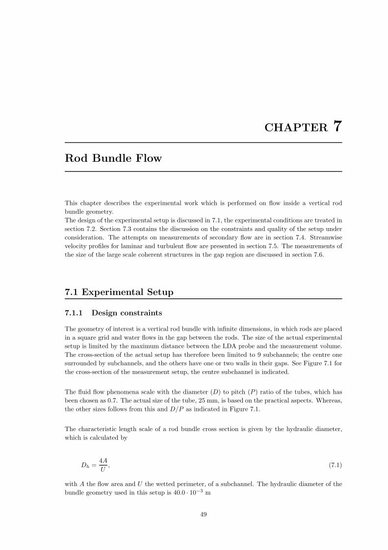
CHAPTER 7
Rod Bundle Flow
This chapter describes the experimental work which is performed on flow inside a vertical rod
bundle geometry.
The design of the experimental setup is discussed in 7.1, the experimental conditions are treated in
section 7.2. Section 7.3 contains the discussion on the constraints and quality of the setup under
consideration. The attempts on measurements of secondary flow are in section 7.4. Streamwise
velocity profiles for laminar and turbulent flow are presented in section 7.5. The measurements of
the size of the large scale coherent structures in the gap region are discussed in section 7.6.
7.1 Experimental Setup
7.1.1 Design constraints
The geometry of interest is a vertical rod bundle with infinite dimensions, in which rods are placed
in a square grid and water flows in the gap between the rods. The size of the actual experimental
setup is limited by the maximum distance between the LDA probe and the measurement volume.
The cross-section of the actual setup has therefore been limited to 9 subchannels; the centre one
surrounded by subchannels, and the others have one or two walls in their gaps. See Figure 7.1 for
the cross-section of the measurement setup, the centre subchannel is indicated.
The fluid flow phenomena scale with the diameter (D) to pitch (P ) ratio of the tubes, which has
been chosen as 0.7. The actual size of the tube, 25 mm, is based on the practical aspects. Whereas,
the other sizes follows from this and D/P as indicated in Figure 7.1.
The characteristic length scale of a rod bundle cross section is given by the hydraulic diameter,
which is calculated by
Dh =4A
U, (7.1)
with A the flow area and U the wetted perimeter, of a subchannel. The hydraulic diameter of the
bundle geometry used in this setup is 40.0 · 10−3 m
49
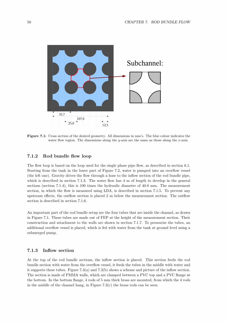
50 CHAPTER 7. ROD BUNDLE FLOW
Figure 7.1: Cross section of the desired geometry. All dimensions in mm’s. The blue colour indicates thewater flow region. The dimensions along the y-axis are the same as those along the x-axis.
7.1.2 Rod bundle flow loop
The flow loop is based on the loop used for the single phase pipe flow, as described in section 6.1.
Starting from the tank in the lower part of Figure 7.2, water is pumped into an overflow vessel
(the left one). Gravity drives the flow through a hose to the inflow section of the rod bundle pipe,
which is described in section 7.1.3. The water flow has 4 m of length to develop in the general
sections (section 7.1.4), this is 100 times the hydraulic diameter of 40.0 mm. The measurement
section, in which the flow is measured using LDA, is described in section 7.1.5. To prevent any
upstream effects, the outflow section is placed 2 m below the measurement section. The outflow
section is described in section 7.1.6.
An important part of the rod bundle setup are the four tubes that are inside the channel, as drawn
in Figure 7.1. These tubes are made out of FEP at the height of the measurement section. Their
construction and attachment to the walls are shown in section 7.1.7. To pressurise the tubes, an
additional overflow vessel is placed, which is fed with water from the tank at ground level using a
submerged pump.
7.1.3 Inflow section
At the top of the rod bundle sections, the inflow section is placed. This section feeds the rod
bundle section with water from the overflow vessel, it feeds the tubes in the middle with water and
it supports these tubes. Figure 7.3(a) and 7.3(b) shows a scheme and picture of the inflow section.
The section is made of PMMA walls, which are clamped between a PVC top and a PVC flange at
the bottom. In the bottom flange, 4 rods of 5 mm thick brass are mounted, from which the 4 rods
in the middle of the channel hang, in Figure 7.3(c) the brass rods can be seen.
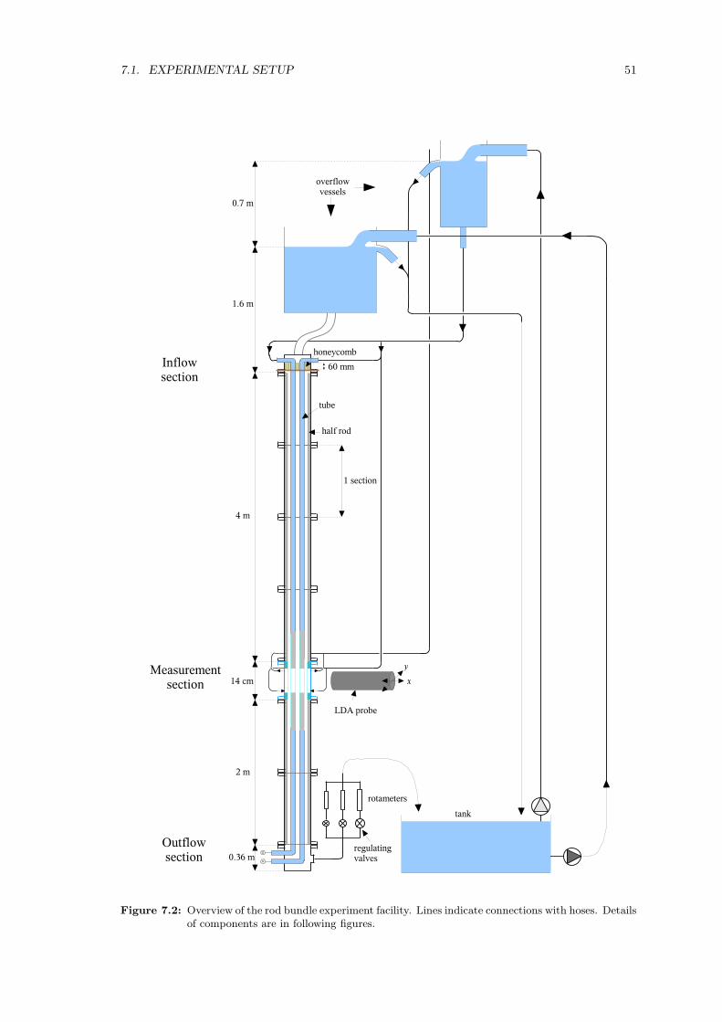
7.1. EXPERIMENTAL SETUP 51
Figure 7.2: Overview of the rod bundle experiment facility. Lines indicate connections with hoses. Detailsof components are in following figures.

52 CHAPTER 7. ROD BUNDLE FLOW
The inflow section is important for straightening the flow, and tripping the fluid to create tur-
bulence. To this end, a honeycomb structure is placed above the brass rods, with a height of 60
mm and a mesh size of 0.6 cm. This removes almost all swirling and horizontal movement of the
water flow. Downstream, rubber O-rings with 2 mm diameter are placed around the tubes in the
centre, applying a sudden narrowing of the flow which onsets turbulence. The brass rods also
account in this process.
(a) (b)
(c) (d)
Figure 7.3: Schemes and graphs of the inflow section. (a) and (b) show a side-view, (c) and (d) a topview.
7.1.4 General sections
The rod bundle tube consists of 6 pieces of 1.0 m in length made of poly vinyl chloride (PVC)
and 1 piece of 14 cm in length made of poly methyl methacrylate (PMMA). The latter one is the
measurement section and is treated in section 7.1.5. The PVC parts consist of flat plates with a
thickness of 10 mm, glued together to a box. The rods attached to the wall are made of solid PVC
rods, that are glued in milled slits, see Figure 7.4(a).
The connection between the different tube segments is made by flanges, that are water-tightened

7.1. EXPERIMENTAL SETUP 53
using O-rings. At the transitions between the different segments, there might be a step in the wall
along the axial direction. This step could not be measured directly, but an optical investigation
did not show steps larger than 0.5 mm. In appendix D.2 and D.3 a description is given of a
backward-facing step and a forward-facing step. The vortices reattach at a maximum of 3.5 mm
behind the step, so these irregularities should not have an effect on the results.
One of the PVC sections is shown in Figure 7.4(b).
The shape of the PVC parts is not exactly the same as the desired geometry, compare Figures
7.4(a) and 7.1. The rods used in the PVC section had a diameter of 25.6 mm instead of 25.0,
which gives them a base that is too wide. The effects of this on the flow should however be limited,
because the maximum difference is a narrowing of 0.5 mm of the gaps that are next to a wall.
(a) Scheme of the cross-section of bundlegeometry for the PVC-parts
(b) Picture of 1 m section, made of PVC with semi and quarterrods attached to the wall.
Figure 7.4
7.1.5 Measurement section
The measurement section has the same proportions as the normal PVC sections, but is mainly
made of transparent material. The square casing consists of 9 mm thick PMMA plates, the flanges
are made of PMMA as well. The rods which are opposite from the probe position, are made out
of PVC, since there is no need for them to be transparent. The cross section of the measurement
section is drawn in Figure 7.5(a) and a photograph of the top can be found in Figure 7.5(b).
The semi and quarter cylinders are made out of FEP, to avoid unwanted diffractions from its curved
surfaces. As can be concluded from chapter 5, there is a need to make the FEP tubes as thin as
possible. The FEP tubes were shrunk over PTFE, see Appendix C for details, and mounted to
the wall by clamping them over PMMA solid rods, as is explained in Appendix C.3.2. To keep the
thin-wall FEP tubes in shape, they have to be filled with water, which has a slight overpressure
with respect to the water.
LDA traversing system
The LDA probe is placed on a 2 dimensional traversing table, which can move in the plane of the
cross section of the rod bundle tube. The table is placed at a constant height, such that all laser
beams needed for the LDA cross the FEP pipe parts.

54 CHAPTER 7. ROD BUNDLE FLOW
(a) Cross-section of the bundle geometry for the mea-surement section. Light blue indicates PMMA, greyPVC and dark blue FEP.
(b) Top view of the measurement section.
Figure 7.5
7.1.6 Outflow section
The rod-bundle cross-section remains the same until two meters below the measurement section,
to prevent upstream effects of the outflow of fluid. The outflow section itself consists of a box
below the lowest PVC rod-bundle section. The fluid flowing along the rods flows out by a large
hose at one side, and the inner tubes are separately connected to a tap at the outside.
7.1.7 Tubes and spacers
Tubes
The four tubes that are at the inside of the rod bundle cross section, consist of three parts. From
top to bottom, the first 3.9 m are made of PVC, the next 60 cm are made of stainless steel with
FEP and the lowest 1.9 m is made of PVC as well. The PVC parts are made of PVC tubes with
an outer diameter of 25.00 mm and 1.9 mm thick walls.
The stainless steel tubes with FEP section, which is at the height of the measurement section,
consists of two stainless steel pipes of 30 cm in length, with a FEP tube shrunk over them. Between
the two stainless steel tubes, a section of 6 cm remains clear of stainles steel, as is indicated in
Figure 7.6. These tubes were manufactured using a PTFE mold, as is described in Appendix C.2
and have an outer diameter of 25.0 mm, which is connected to the PVC tubes with a smooth
connection.
Spacers
The four tubes that are in the centre of the rod-bundle cross section, need to be at the correct
position, in a regular grid. Due to the fluid flow and possible irregularities in the tubes they will
not automatically hang straight from their support at the inflow section.

7.1. EXPERIMENTAL SETUP 55
(a) photograph
(b) scheme
Figure 7.6: Inner tube
At almost each flange, except for the one just above and just below the measurement section, a
spacer grid is placed. These grids consist of a rectangular PVC frame with four horizontal and
four vertical wires, like in Figure 7.7.
The wires should not disturb the flow too much, but should also be strong enough to keep the
tubes into their position. As a compromise, the stainless steel wires have a diameter of 1 mm,
which creates noticeable vortices up to 30 cm (see Appendix D.1). To obtain more rigidity, the
wires are point welded at the crossings.
Figure 7.7: Scheme of a spacer.
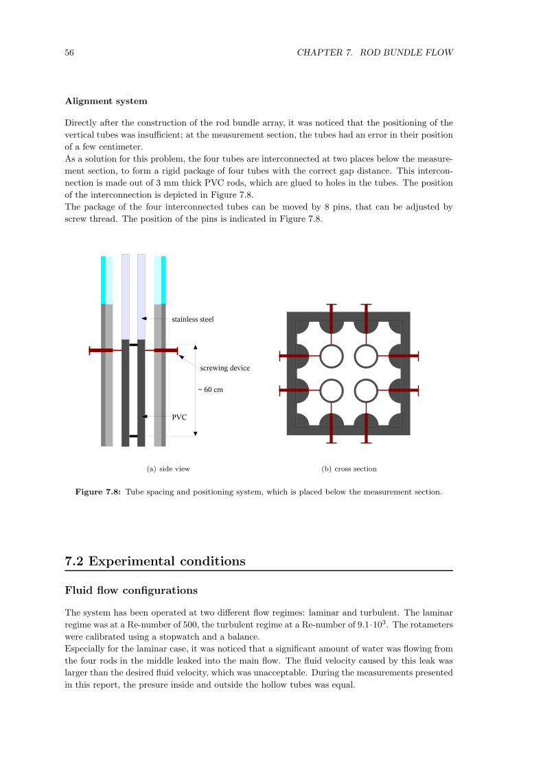
56 CHAPTER 7. ROD BUNDLE FLOW
Alignment system
Directly after the construction of the rod bundle array, it was noticed that the positioning of the
vertical tubes was insufficient; at the measurement section, the tubes had an error in their position
of a few centimeter.
As a solution for this problem, the four tubes are interconnected at two places below the measure-
ment section, to form a rigid package of four tubes with the correct gap distance. This intercon-
nection is made out of 3 mm thick PVC rods, which are glued to holes in the tubes. The position
of the interconnection is depicted in Figure 7.8.
The package of the four interconnected tubes can be moved by 8 pins, that can be adjusted by
screw thread. The position of the pins is indicated in Figure 7.8.
(a) side view (b) cross section
Figure 7.8: Tube spacing and positioning system, which is placed below the measurement section.
7.2 Experimental conditions
Fluid flow configurations
The system has been operated at two different flow regimes: laminar and turbulent. The laminar
regime was at a Re-number of 500, the turbulent regime at a Re-number of 9.1·103. The rotameters
were calibrated using a stopwatch and a balance.
Especially for the laminar case, it was noticed that a significant amount of water was flowing from
the four rods in the middle leaked into the main flow. The fluid velocity caused by this leak was
larger than the desired fluid velocity, which was unacceptable. During the measurements presented
in this report, the presure inside and outside the hollow tubes was equal.

7.2. EXPERIMENTAL CONDITIONS 57
During a measurement set, the temperature of the water increased by the heat of the pump. The
typical increase was limited to 1. For a typical increase from 19 C to 20 C the viscosity decreased
from 1.03 ·10−6 to 1.007 ·10−6 m2
s , increasing the Reynolds number by 2%. No correction has been
made for this, because the flow control can not set these small differences accurately.
Laser probe alignment
The axial velocity component is measured using the blue beams of the LDA probe and the hor-
izontal velocity components using the green beams, recall section 3.5. The fluid velocity in the
horizontal plane is of special interest, because cross flow is in that direction. But the horizontal
component of the velocity is very small, in the order of 1 % of the streamwise velocity. If the
laser probe is not properly aligned, the measurements of the horizontal velocity are ‘biased’ by the
streamwise velocity; an error of 1 leads to a bias of 1.74 % of the streamwise velocity.
The alignment of the laser probe is carried out in various steps:
• The probe is levelled using a levelling rod in the plane of the cross section of the rod bundle
tube.
• The rotation of the probe around its axis is set by pointing the vertical (blue) bundles parallel
to the wall of the rod bundle casing.
• The axis of the probe is made parallel to the wall of the measurement section.
The steps above should make sure that an unbiased secondary flow can be measured. Not all tubes
in the rod bundle setup are perfectly parallel, introducing a movement of fluid in the direction
normal to the streamwise direction.
Although it is known to the author that the position and angle of the tubes severely effects the
secondary flow, the probe is rotated in such a way that the blue beams are parallel to the stream-
wise direction of the flow. This was performed by setting the horizontal velocity component equal
to zero in a laminar flow. The required rotation of the probe around its axis was about 1. This
calibration needs to be redone for the different positions in the cross section of the rod bundle,
indicating that the different tubes are not parallel to each other.
As a measure for the quality of alignment, we introduce the RMS value for the horizontal ve-
locity, which should be 0 by theory for laminar flow:
error =1
N
N∑
i=1
√(
vx
vz
)2
, (7.2)
with vx the measured velocity in the horizontal plane and vz the measured velocity in the axial
direction.
LDA settings
The system is operated at two different Reynolds numbers: 500 (laminar) and 9.1 ·103 (turbulent).
Each velocity requires its own settings for the Color Link and IFA due to the different Doppler
frequency shift, see section 3.2. Applying the settings in Table 7.1 gives in general a sufficient
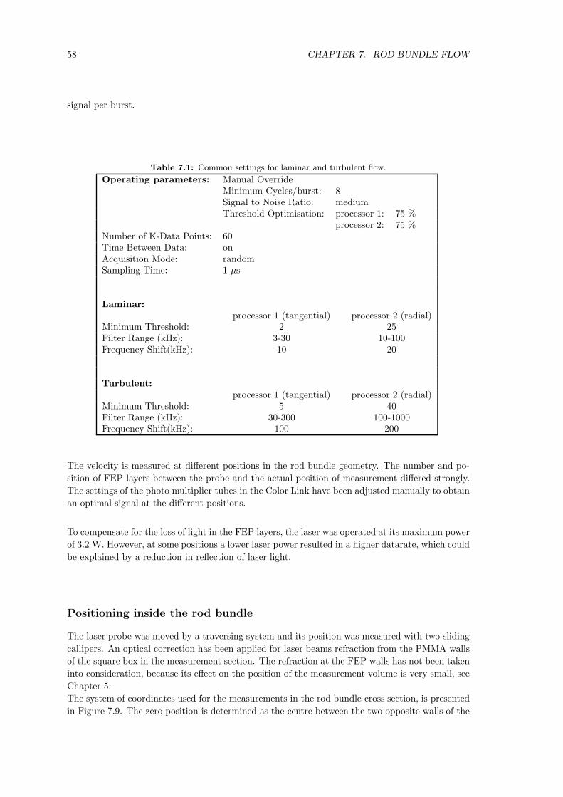
58 CHAPTER 7. ROD BUNDLE FLOW
signal per burst.
Table 7.1: Common settings for laminar and turbulent flow.
Operating parameters: Manual OverrideMinimum Cycles/burst: 8Signal to Noise Ratio: mediumThreshold Optimisation: processor 1: 75 %
processor 2: 75 %Number of K-Data Points: 60Time Between Data: onAcquisition Mode: randomSampling Time: 1 µs
Laminar:
processor 1 (tangential) processor 2 (radial)Minimum Threshold: 2 25Filter Range (kHz): 3-30 10-100Frequency Shift(kHz): 10 20
Turbulent:
processor 1 (tangential) processor 2 (radial)Minimum Threshold: 5 40Filter Range (kHz): 30-300 100-1000Frequency Shift(kHz): 100 200
The velocity is measured at different positions in the rod bundle geometry. The number and po-
sition of FEP layers between the probe and the actual position of measurement differed strongly.
The settings of the photo multiplier tubes in the Color Link have been adjusted manually to obtain
an optimal signal at the different positions.
To compensate for the loss of light in the FEP layers, the laser was operated at its maximum power
of 3.2 W. However, at some positions a lower laser power resulted in a higher datarate, which could
be explained by a reduction in reflection of laser light.
Positioning inside the rod bundle
The laser probe was moved by a traversing system and its position was measured with two sliding
callipers. An optical correction has been applied for laser beams refraction from the PMMA walls
of the square box in the measurement section. The refraction at the FEP walls has not been taken
into consideration, because its effect on the position of the measurement volume is very small, see
Chapter 5.
The system of coordinates used for the measurements in the rod bundle cross section, is presented
in Figure 7.9. The zero position is determined as the centre between the two opposite walls of the

7.3. QUALITY OF THE SETUP 59
square box in the measurement section. These wall positions are measured in two ways:
• The wall positions over the x-axis are measured by finding the position where the blue laser
beams cross transparent FEP tubes that are attached to the wall.
• For the y-axis, the positions of the wall are found by measuring the velocity along the y-axis
for laminar flow, and extrapolating these samples to zero velocity.
Figure 7.9: Reference frame in the rod bundle cross section. The origin is centred with respect to thewalls of the square.
7.3 Quality of the setup
7.3.1 Positions of tubes
An appropriate alignment and positioning of the vertical tubes is of great importance for accurate
measurements. Various methods for determining the tube wall positions have been examined, these
are:
• The crossing of the four laser beams (two green and two blue ones) forms the measurement
volume. The human eye can observe the position at which the crossing beams just enter the
wall. However, this method did not have a high reproduceability. Based on the differences in
subsequent results for the same position measurement, the error in the results is estimated
to be about 2 mm, which is insufficient.
• When the measurement volume overlaps with the wall, the LDA signal shows an increase in
noise level. The amplitude of the noise depends on the light intensity of the measurement
volume that is inside the wall. However, in some regions already have high background noise

60 CHAPTER 7. ROD BUNDLE FLOW
levels, due to multiple layers of FEP between the probe and the measurement volume.
The measurement volume has a size in the x-direction of 0.03 mm and in the y-direction
of 0.2 mm (section 3.3.5). The combined effect of a gradual increase in noise and high
level of background noise, makes the error of this solution in the order of 1 mm, based on
reproduceability of the results.
• For a laminar flow, the axial velocity can be measured. Laminar flow shows a parabolically
shaped velocity profile. A set of streamwise velocity measurements on a line in the gap region
can be used to fit a parabola through. The zero-crossings of the parabola indicate the walls
of the tubes, an example of this is shown in Figure 7.10
This method resulted in very reproduceable results and because of the viscous regime, the
geometry has a major influence on the flow. Using error regression theory, the uncertainty
(∆y) in the fitted parabola can be used to estimate the uncertainty in the wall position (∆x):
∆x =∂f
∂y∆y =
±1
2√
y∆y where f(y) = ±√
y. (7.3)
For the most erroneous position, ∆y = 0.025 mm and y = ±6 mm, which results in a
maximum error in the tube position of 0.16 mm.
Figure 7.10: Axial velocity profile for a laminar flow, over the line y = 20.00. The wall positions are thezero crossings of the parabolic fit.
The last method was used to map all the tubes in the cross section of the flow area. These re-
sults are depicted in Figure 7.11. Circles have been fitted to the measured wall positions, under
assumption that the tubes maintained their original circular shape with an outer diameter of 25
mm. Since all measured points are within 1 mm of the fitted circle, this seems to be a reasonable
assumption.
Based on Figure 7.11, the tubes appear to be off centred when compared with the ideal geometry
(Figure 7.1).
The error in their position, is such that it seriously affects the flow and makes comparison with
literature impossible. With the present setup it was not possible to improve the quality of the
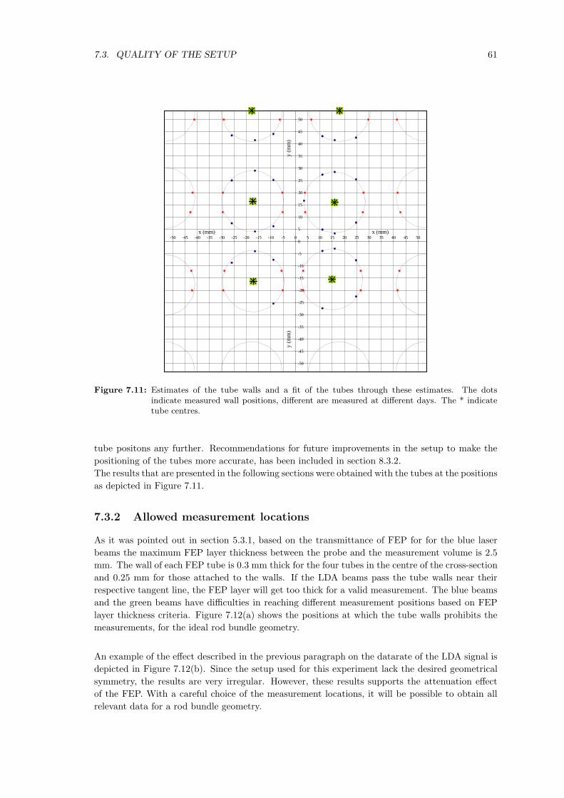
7.3. QUALITY OF THE SETUP 61
Figure 7.11: Estimates of the tube walls and a fit of the tubes through these estimates. The dotsindicate measured wall positions, different are measured at different days. The * indicatetube centres.
tube positons any further. Recommendations for future improvements in the setup to make the
positioning of the tubes more accurate, has been included in section 8.3.2.
The results that are presented in the following sections were obtained with the tubes at the positions
as depicted in Figure 7.11.
7.3.2 Allowed measurement locations
As it was pointed out in section 5.3.1, based on the transmittance of FEP for for the blue laser
beams the maximum FEP layer thickness between the probe and the measurement volume is 2.5
mm. The wall of each FEP tube is 0.3 mm thick for the four tubes in the centre of the cross-section
and 0.25 mm for those attached to the walls. If the LDA beams pass the tube walls near their
respective tangent line, the FEP layer will get too thick for a valid measurement. The blue beams
and the green beams have difficulties in reaching different measurement positions based on FEP
layer thickness criteria. Figure 7.12(a) shows the positions at which the tube walls prohibits the
measurements, for the ideal rod bundle geometry.
An example of the effect described in the previous paragraph on the datarate of the LDA signal is
depicted in Figure 7.12(b). Since the setup used for this experiment lack the desired geometrical
symmetry, the results are very irregular. However, these results supports the attenuation effect
of the FEP. With a careful choice of the measurement locations, it will be possible to obtain all
relevant data for a rod bundle geometry.

62 CHAPTER 7. ROD BUNDLE FLOW
The measurements, as presented in section 5.3.1, indicate that a FEP layer of 1.5 mm would
return a high datarate. However, when the FEP of 2.5 mm thickness consists of different layers
with space in between, like in the rod bundle setup, the signal is become attenuated. As a practical
consequence, the three subchannels with the largest distance to the probe (beyond y − 25.0), can
not be investigated with the LDA technique.
(a) Lines on which the data rate will be very low.The green lines are the locations for the horizontalvelocity and the blue beams the locations for the axialvelocity.
(b) Data-rate on the line y = 0.00 mm for the greenbeams and blue beams, indicated by colour.
Figure 7.12: Allowed measurement locations and example
7.3.3 Refractive index mismatch
The difference in refractive index between FEP and water is very small (see section 5.3.1), how-
ever some refractive effects will allways be there. Refraction is important with respect to two
measurement considerations:
• Refraction will make it difficult to know the location of the measurement volume.
• If the two measurement volumes are shifted, the correlation between the axial and horizontal
velocity components is lost.
The effects of refraction in the rod bundle geometry have been investigated in two ways: (i) by
measuring the refraction over the complete geometry and (ii) by measuring the overlap of the
measurement volumes for two different colours.

7.3. QUALITY OF THE SETUP 63
Direct refraction measurement
There is always some refraction of laser light by walls of the FEP tubes. It is not possible to
measure the angle of refraction of a single tube inside the geometry, only measurements of the
complete geometry are possible. These measurements are limited by the PVC semi-tubes which
are attached to the back wall of the rod bundle cross-section, see Figure 7.5(a). The effect of
refraction on the horizontal beam position can therefore not be measured, these beams will be
blocked by the PVC after passing through the FEP tubes.
The angle of the beams used for the horizontal velocity components (the green beams) was mea-
sured at positions where these beams could pass through the gap between the PVC tubes. Within
the precision of the measurement, the beams leaving the rod bundle had the same angle with
respect to the probes lens as the beams entering the rod bundle, i.e. 10.7.
Overlap of measurement volumes
The measurement volume for one flow direction, is formed by the crossing of its two respective
beams. Each beam pair is refracted differently by the FEP wall, since they cross different FEP
tubes at different angles. Refraction effects can therefore cause the two measurement volumes to
be at different positions.
When the two measurement volumes overlap, a particle that is detected by one beam pair will
also be detected by the other (under the assumption that no other effects distort the measurement
for one of the two beam pairs). When the measurement volumes overlap partly, not all particles
detected in one colour beam pair will also result in a detection in the other colour. The ratio
between the particles detected by both colours beam pairs to the particles detected in just one
colour beam pair, is a measure for the overlap of both the measurement volumes and can be
interpreted as
fcoincidence
fall,
∫
A ∩ B
I(x, y) dx dy (7.4)
with f the datarate, A and B the respective directions of measurement, I the intensity of light in
a measurement volume.
An example of the coincidence at different points is given in Figure 7.13(a). The datarate of
particles seen by both colours is divided by the datarate of the blue beams. Blue is chosen because
it produces a lower datarate than green. Using this method, all points that are measured in the
rod bundle are checked for coincidence, see Figure 7.13(b). The threshold of an overlap was chosen
to be 0.2. The measurement volume length in the y-direction is 0.2 mm and the width in the
x-direction is 0.03 mm (section 3.3.5). This makes it more likely that the position shift detected
by the coincidence criterion is caused by a shift in the x-direction. The overlap threshold of 0.2
means a distance of 25 µm ((1 - 0.8) × 0.03 mm) in the x-direction.
The overlap threshold was chosen using the criterion that the two measurement volumes should be
within the size one of the smallest vortices. Using the Kolmogorov Microscale, defined in Appendix
A.1, the smallest eddy size was calculated to be 1.5 mm, based on u′ ≈ 0.002 m/s and Dh as length
scale. The distance between the two measurement volumes at the threshold level is about 1% of the

64 CHAPTER 7. ROD BUNDLE FLOW
(a) Overlap of two measurement volumes as a function of y over line x = -10.0 mm, based onbursts detected at the same moment.
(b) Cross section of the rod bundle, each measurement location is indicatedwith a blue dot. If the blue and green measurement volume had an overlap ofless then 20 %, the spot is marked red.
Figure 7.13

7.4. SECONDARY FLOW 65
microscala size; the correlation between the axial and horizontal velocity components is therefore
a useful measure when the minimum overlap of 0.2 as criterion is applied.
7.4 Secondary Flow
The secondary flow pattern in the rod bundle subchannel, is one of the interesting flow phenomena,
as it is discussed in section 2.2. According to Ikeno and Kajishima [32], the secondary flow for a
subchannel with a diameter over pitch ratio of 0.7 is in the order of 0.5 % of the streamwise flow
at maximum.
The horizontal velocity component has been measured at points along different lines in our rod
bundle facility. As it was mentioned in section 7.2, the probe was rotated around its axis to obtain
a horizontal velocity component equal to zero. However, there was no rotation possible such that
the laminar horizontal velocity component was zero for all positions in the cross section. Therefore,
the probe was aligned for an almost zero horizontal velocity in the middle of each measurement
set for laminar flow conditions. The most likely cause for this effect is that the vertical tubes do
not have the same cross-sectional position at each height, resulting in oblique tubes and causing a
non zero horizontal velocity.
The alignment resulted in a slightly different quality then indicated in section 7.2, because it is
optimised for the local orientation of the bundle. Expressed in RMS value of the horizontal ve-
locity, values were obtained for the line y = 17.46 mm for the centre gap. For laminar flow (Re
≈ 500), the RMS value for the horizontal flow was 0.3 % of the streamwise flow and for turbulent
(Re=9100) flow, the RMS value for the horizontal velocity was 0.7 %.
Figures 7.14 and 7.15 show the results for the horizontal velocity for lines with constant y and
x respectively. The LES simulation of Ikeno and Kajishima [32] is shown as reference. Although
it might be possible to recognise some correspondence between the literature and current work,
the amplitude of the horizontal velocity which is measured, is probably far too large. This can
be explained by the obliqueness of the tubes; an angle of 1 will introduce a bias of 1.75 % of
the streamwise flow, which is in the order of 0.25 v+. The results obtained for the horizontal
flow therefore are not very helpful in understanding the secondary flow. To obtain usable results,
further modifications in the setup are required, as discussed in section 8.3.2.
7.5 Flow profiles
The rod bundle facility has been investigated with different flow regimes. The first case to examine
was the well known laminar flow (Re = 500), , for which no horizontal flow is expected. The laminar
results are given in section 7.5.1. The measurements for the turbulent regime were obtained at Re
= 9100. Interesting flow properties of the turbulent flow are the turbulence characteristics and the
friction velocity, these can be found in section 7.5.2
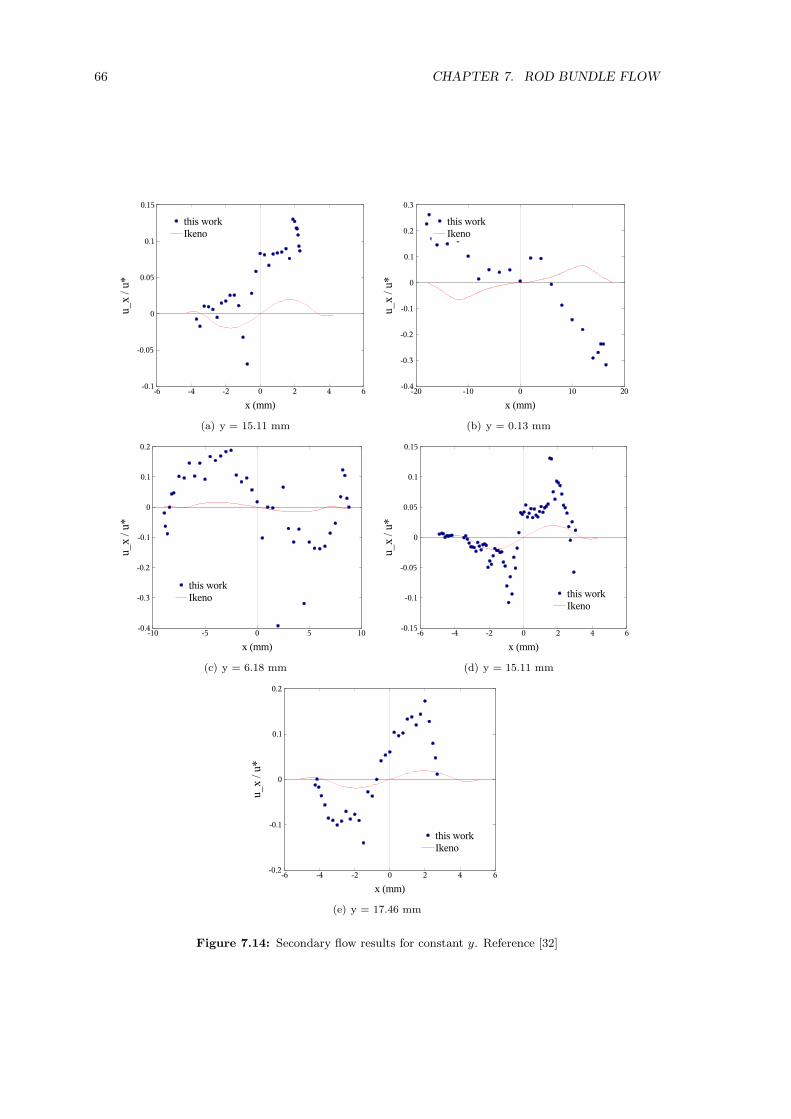
66 CHAPTER 7. ROD BUNDLE FLOW
(a) y = 15.11 mm (b) y = 0.13 mm
(c) y = 6.18 mm (d) y = 15.11 mm
(e) y = 17.46 mm
Figure 7.14: Secondary flow results for constant y. Reference [32]

7.5. FLOW PROFILES 67
(a) x = -17.85 mm (b) x = -9.00 mm
(c) x = 7.50 mm (d) x = 15.00 mm
Figure 7.15: Secondary flow results for constant x. Reference [32]

68 CHAPTER 7. ROD BUNDLE FLOW
7.5.1 Laminar
The streamwise velocity has been measured along the two symmetry axes of the setup. These
results are shown in Figure 7.16, where they are compared to a numerical simulation of a single
subchannel using Fluent.
It is noted that the shape of the curve resembles the simulation, but the measured velocity in the
centre is much too low. This can be explained by the imperfect location of the tubes in the cross
section of the setup, which reduces the size of the subchannel in the centre, and the chosen line
does not cross the centre of all subchannels.
The horizontal velocity is not depicted in the Figure, but for the best possible alignment, its
RMS-value for the line x = 0.00 mm was 1.92 % of the streamwise flow and for the line y = 0.00
mm 1.96 % of the streamwise flow. For laminar flow, no horizontal flow is expected and this effect
must therefore be due to the oblique placement of the tubes.
Figure 7.16: Axial velocity over two lines for laminar flow. Fluent simulation data is over the centre-lineof an ideal subchannel.
7.5.2 Turbulent
Just like for the laminar flow, the streamwise velocity has been measured for the turbulent (Re =
9100) case. Its results are depicted in Figure 7.17. It should be remarked to the reader that the v∗
was derived from the ∂uz/∂x value in the viscous sublayer, obtained on different days. This could
explain the higher velocity for the profile along the line y = 0 mm. For comparison, reference data
is shown of Ikeno and Kajishima [32], which was calculated using LES.
The results show a good resemblance with the reference data, with respect to the measured velocity
and shape of the curve. A shift in the position of the maximum is explained by considering the
centre of the subchannel that is not exactly at the point x = 0.00 mm and y = 0.00 mm.

7.5. FLOW PROFILES 69
Figure 7.17: Results for the axial velocity in the middle subchannel for Re = 9100, numerical data fromIkeno and Kajishima [32].
The velocity in the gap region at y ≈ 15 mm which is significantly lower than the simulation
is caused by the tube wall which is closer to the measurement position in the setup than in the
simulation.
Turbulence kinetic energy
The turbulence intensities u′xu′
x, u′xu′
z and u′zu
′z are a measure for the transport of kinetic energy
in a turbulent flow. In two gaps with a different orientation, the turbulence intensities have been
measured and studied, see Figure 7.18. For comparison, the LES results of Ikeno and Kajishima
[32] are depicted. There is a difference in the u′xu′
x term in Figures 7.18(a) and 7.18(b): for the
first, the horizontal velocity component measured is parallel to the line along the gap, for Figure
7.18(b) the horizontal velocity component is perpendicular to the line along the gap.
The higher noise level in Figure 7.18(b) can be explained by a lower sampling frequency for both
colours than for the other Figure. Typically, the datarate was 2 Hz for x = −17.00 mm and more
than 10 Hz for y = −17.46 mm.
As stated in the previous section, the tubes are not fully parallel in the streamwise direction. After
a change in cross-sectional geometry, the flow needs some length to redevelop again, which can be
considered as restoring the kinetic energy distribution. When considering
√
(u′z)
2 for y = 17.46
mm, an asymmetry can be seen; the maximum around x = −3.5 mm is much wider than at the
other side. To restore the equilibrium, kinetic energy needs to be transferred to the other side, a
process which seems to be going on already considering the higher value of
√
(u′z)
2 in the centre
of the gap.
For a pipe, the u′ru
′z term can be used to calculate the friction velocity, as explained in Appendix
B. To apply the same method to the rod bundle geometry is very difficult, since in equation B.4,
the term ux is not equal to 0, because of a velocity component in the horizontal direction for the
centre of the gap. The current setup has however a relatively strong flow in the horizontal direction
caused by the pipe positions. With a setup in which the secondary flow can be measured and with
a zero time-averaged horizontal flow component in the centre of the gap, this method should be
usable again.

70 CHAPTER 7. ROD BUNDLE FLOW
(a) y = 17.46 mm (b) x = −17.00 mm
Figure 7.18: Turbulence intensities. LES results by Ikeno and Kajishima [32].
Friction velocity
To measure the friction velocity v∗ and to determine the quality of the measurement technique
with respect to near wall measurements, the axial velocity component has been determined at
different positions in the cross section of the rod bundle.
It is important to bear in mind that the measurement volume for the LDA system used, has
a length of 0.21 mm in the y-direction and a with of 0.03 mm in the x-direction, see section 3.3.5.
Therefore, a higher spatial resolution can be obtained in the x-direction.
The first near wall measurement were done along the x-direction, at a place where no FEP was
between the measurement volume and the probe. These results are given in Figure 7.19(a) and it
shows that measurements at less than y+ = 1 are possible, where a minimum sampling rate of 0.5
Hz is found. The friction velocity as derived from the ∂uz
∂y is 0.016 m/s, which is the same as Ikeno
and Kajishima [32] used for the LES simulation.
The same procedure has been repeated for a place where there are two FEP layers between the
probe and the measurement volume. Those results are shown in Figure 7.19(b). More noise and
a lower datarate is observed. The sampling frequency at y+ = 3 is 0.2 Hz, indicating that mea-
surements as close to the wall as these are still feasible. The points closer to the wall confirm the
trend of the viscous sublayer, but are based on just a few bursts (fsample ≈ 0.05 Hz).
The friction velocity for this measurement set is 0.016 m/s, with a higher uncertainty than the
previous measurement.
Near wall measurements were also performed for the tube with centrepoint (14.9,-15.5) mm over a
line with an angle with respect to the x-axis towards the positive y-axis. For the angle of 25 the
results are shown in Figure 7.19(c) and for 42 in Figure 7.19(d). For 25 , the friction velocity
was determined to be 0.017 m/s and for 42 0.016 m/s. For these measurements, the green beams
were used for the axial velocity, because they resulted in a higher datarate.
For measuring over the line with an angle of 25, the sampling frequency steadily drops till 0.4 Hz
at y+ = 1.4 and then it increases again, indicating a significant contribution of noise in the signal.
For the 42 case, there is some signal with a sampling frequency of 0.5 Hz till y+ = 4.3 and closer
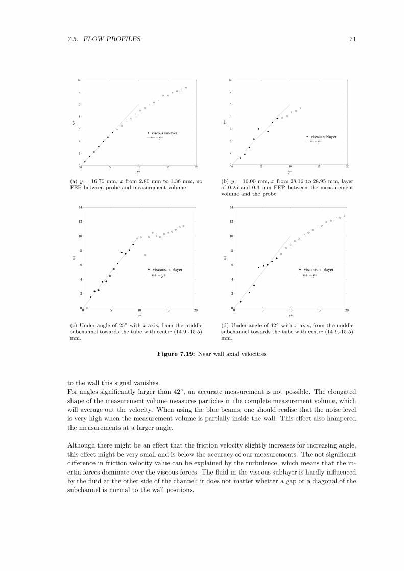
7.5. FLOW PROFILES 71
(a) y = 16.70 mm, x from 2.80 mm to 1.36 mm, noFEP between probe and measurement volume
(b) y = 16.00 mm, x from 28.16 to 28.95 mm, layerof 0.25 and 0.3 mm FEP between the measurementvolume and the probe
(c) Under angle of 25 with x-axis, from the middlesubchannel towards the tube with centre (14.9,-15.5)mm.
(d) Under angle of 42 with x-axis, from the middlesubchannel towards the tube with centre (14.9,-15.5)mm.
Figure 7.19: Near wall axial velocities
to the wall this signal vanishes.
For angles significantly larger than 42, an accurate measurement is not possible. The elongated
shape of the measurement volume measures particles in the complete measurement volume, which
will average out the velocity. When using the blue beams, one should realise that the noise level
is very high when the measurement volume is partially inside the wall. This effect also hampered
the measurements at a larger angle.
Although there might be an effect that the friction velocity slightly increases for increasing angle,
this effect might be very small and is below the accuracy of our measurements. The not significant
difference in friction velocity value can be explained by the turbulence, which means that the in-
ertia forces dominate over the viscous forces. The fluid in the viscous sublayer is hardly influenced
by the fluid at the other side of the channel; it does not matter whetter a gap or a diagonal of the
subchannel is normal to the wall positions.

72 CHAPTER 7. ROD BUNDLE FLOW
7.6 Large scale coherent structures
It is assumed that large scale coherent structures, moving in the streamwise direction, exists
near the gap-region, as discussed in section 2.3. The experimental technique of LDA allows only
correlations in time for a single point and this poses some difficulties in measuring the vortex-
shaped structures. Using Taylor’s hypothesis, it is possible to use the single point time series
measurements to obtain an estimate for the streamwise length of the structures [33]. Taylor’s
hypothesis for this situation is given by:
∂ux
∂t= Uz
∂ux
∂z, (7.5)
which on integration with respect to t and z yields:
Lz = Uz ∆t, (7.6)
with Lz the length of the structure in the z-direction, Uz the structure velocity and ∆t the time one
structure lasts at the measurement position, which in a correlation graph is the time lag between
two maxima in correlation. Using this definition, the streamwise length Lz of a structure is defined
as in Figure 7.20(a), the distance from a structure centre to the next structure centre.
The structure size has been measured using Taylor’s hypothesis for different Re-numbers. To
do this, the correlation function for a point in the gap region was calculated using the fuzzy slot-
ting technique (section 4.3.5). In this correlation function, the time lag between t=0 and the first
positive maximum was determined, or the time lag between the first and the second minimum, see
Figure 7.20(b).
Mahmood et al. [1] investigated the structure size and velocity using Particle Image Velocimetry
(PIV) and found that the structure velocity was nearly equal to the streamwise velocity in the
centre of the subchannel. For that reason, in this research the highest velocity in the centre of the
subchannel is used for the calculation of the structure size.
The results for the structure size estimation are depicted in Figure 7.21. For very low Reynolds
numbers, the structure sizes is very long, which shows good resemblance with the reference data,
which was obtained in a simplified geometry using PIV.
To obtain a prediction for the results using the current experimental results, a function was cal-
culated based on a linear fit of the sub channel centre velocity as function of the Re number,
and of 1/τ . Both fits showed a clear difference between the laminar and turbulent regime, with a
transition at Re = 2000. The product of both functions (τ times Ux) is plotted in Figure 7.21.
Summary
• A rod bundle geometry with DP = 0.7 is constructed and its properties are investigated.
The tubes are not at the ideal positions and not parallel, which disturbs horizontal velocity
measurements.

7.6. LARGE SCALE COHERENT STRUCTURES 73
(a) Definition of the structurelength.
(b) Correlation function at Re = 5275 at x= -16.00 mm and y = -0.15mm, time lag τ is indicated.
Figure 7.20: Information about correlation functions
Figure 7.21: Structure sizes as as function of the Reynolds number. Reference data of Mahmood et al.[1].

74 CHAPTER 7. ROD BUNDLE FLOW
• For walls with a normal direction perpendicular the viscous sublayer can be investigated as
close as y+ = 1.
• Large scale flow structures in the gap region are investigated using Taylor’s hypothesis, and
these show good correspondence with literature data.

CHAPTER 8
Conclusions and Recommendations
8.1 Conclusions
The objective of this work was to investigate cross flow in a rod bundle geometry. This was done
using FEP, which is a refractive index matched material to water. The properies of FEP and its
possibilities were investigated in two case studies: a turbulent single phase pipe flow and in a rod
bundle geometry. These results are of use for experiments with other geometries than rectangular
of cylindrical pipes.
The experimental work provided more insight in large scale coherent structures in the gap region of
a rod bundle flow. Due to limitations in the experimental setup, possibilities of comparing velocity
data with literature were limited.
FEP as refractive index matched material
The refractive index of FEP was measured to be 1.341 at ambient conditions, whereas water’s
refractive index is 1.338. This ensures little refraction of light from FEP walls that are not per-
pendicular to the measurement probe axis.
The attenuation of FEP is stronger for light with a shorter wavelength. LDA measurements
through 2.5 mm of FEP or more are not possible due to absorption of light. For different layers
with some space in between, the maximum FEP layer thickness is reduced further.
Possibilities and limitations of FEP with LDA
FEP was used in two flow geometries to be tested: a single phase turbulent pipe and in a rod
bundle geometry.
For the pipe flow, symmetrical and reproducible results were obtained that compared well with
previous experimental and numerical work. Very near wall measurements were obtained, as close
as y+ = 1 which were possible due to the FEP.
75

76 CHAPTER 8. CONCLUSIONS AND RECOMMENDATIONS
The rod bundle setup did not have the correct geometrical symmetry, due to the difficulties in
the design and building process. It was therefore not possible to compare the results with nu-
merical literature data. Altough the flow velocity, friction velocity and flow profile showed good
comparison.
Almost all locations inside the rod bundle geometry can be reached using LDA, except some lines
where the beams have to cross a FEP tube wall with an angle very close to the tangent line. A low
datarate of recognizable LDA bursts can slow down the measurement process significantly. Due to
a different refraction of the two beam pairs used for the different velocity components, there are
regions in the rod bundle cross section where the two measurement volume doe not overlap, and
therefore, it is not possible to measure the u′xu′
z in that region.
The possibilities of near wall measurements in the rod bundle geometry have been examined exper-
imentally. When the wall normal direction is perpendicular to the LDA probe axis, measurements
as close as y+ = 1 were obtained. For other wall normal directions, the nearest measurement
points are further away, even higher than y+ = 10 due to the elongated shape of the measurement
volume. This same problem occurs in geometries constructed out of different materials.
Characteristics of rod bundle geometry
The design and building of a rod bundle geometry setup is difficult due to its large size and high
precision required. The position of the tubes was investigated by fitting a parabolas to measure-
ment sets of laminar profiles. Some tube centres were found to be more than 8 % off their designed
position in terms of pitch distance. Turbulence intensity distributions indicate that the flow is still
at developing stage at the measurement section.
The tubes were not parallel to each other over the full length, which introduced a strong bias
towards the horizontal flow. For laminar flow, the RMS horizontal velocities were more than 1.9
% of the streamwise velocity. This high horizontal bias makes it impossible to measure secondary
flow in the rod bundle geometry.
Rod bundle flow and coherent structures
The presence of large scale coherent structures in the gap region has been investigated. The
horizontal flow showed a periodic behaviour from which a length scale has bee calculated using
Taylor’s hypothesis with the subchannel centre velocity as structure velocity. The results have good
correspondence with literature data. An interesting phenomena is the large size of the structures
for low Re (500).
8.2 Future work
The rod bundle setup used for this project did not have enough precision to measure and investigate
all interesting flow phenomena of a rod bundle geometry. For future work, one could think of the
following interesting research topics:
• Secondary flow; knowledge of the secondary flow field is very important for the transport of

8.3. RECOMMENDATIONS 77
scalars between various subchannels. Furthermore, it forms a good verification of numerical
work.
• Spatial correlations of large scale coherent structures; using Particle Image Velocimetry it is
possible to investigate spatial correlations which could not be done using LDA.
• Scalar transport; injection of a tracer material can be used to gain insight in the inter-channel
transport of scalars by the cross flow.
8.3 Recommendations
8.3.1 Improvement of LDA procedure
• In order to increase fluid flow precision, a more accurate flow meter with better adjustable
valves are recommended.
• The pressure drop has to be calculated from the friction velocity. Measurements of the
pressure drop can form an additional verification of the results.
• The use of newer signal processing equipment could improve the results. The filtering options
of the IFA are limited and that is believed to limit the results. In the rod bundle geometry,
adjustments in the photomultiplier tubes needed to be done to compensate for different levels
of scattered light. In the current setup, this needs to done manually, it is believe that new
Burst detectors can automate this process.
8.3.2 Rod bundle
There are various problems with the present rod bundle geometry that make it impossible to
measure relevant flow data.
• The position of the tubes and hence their distance in between them over the full length is not
correct and introduces a bias in the horizontal velocity measurement and makes its results
useless for comparison.
Tolerance between tube positions should not be greater than 0.1 mm, to ensure the mea-
surements can correspond to literature data. The expected secondary flow is 0.5 % of the
streamwise velocity. With a maximum bias of 10 % of that value, the tubes must be within
0.03 in vertical direction parallel to eachother.
As a solution, the tubes require a fixation closer to the measurement section in the cur-
rent setup. Especially upstream of the measurement section, great care is required to distort
the flow as little as possible Regarding the guidelines given in Appendix D.1, a distance equal
to 300 times the thickness of the spacer wires is advised between the spacer and measurement
section.
In addition, an adjustment system should be incorporated, which enables the bundle geom-
etry to be aligned parallel to the surrounding walls.
78 CHAPTER 8. CONCLUSIONS AND RECOMMENDATIONS
• The FEP tubes are made to be pressurised with 1 m additional hydrostatic water pressure.
Because of some leakage, which is believed to occur at the PVC part of the tubes, or at the
connection between the PVC part and the stainless steel near the FEP, an amount of water
leaks which changes the flow in the measurement section. It is recommended to make the
tubes fully water tight.
Finally, there are some modifications which can simplify the measurements, expand the possibilities
or practical advice:
• For simplicity, 6 of the semi- and quarter rods are made out of PVC. This limits the inves-
tigation of refraction by FEP. It could be considered to make all tubes attached to the wall
out of FEP.
• Near wall measurements can only be done when the wall normal direction is perpendicular
to the probe axis. A probe that could turn around the setup could expand these possibilities.
• The pump heats up the water by approximately 5 C, which changes the density and viscosity.
A temperature control mechanism is advised for maintaining uniform fluid conditions during
the measurements.
• If only the axial velocity is of interest, for example for near wall measurements, it is advised
to use light with a longer wavelength (for example green instead of blue) to obtain a better
datarate.

Acknowledgements
mensen bedanken die onmisbaar zijn geweest tijdens het doen van dit project:
Adtech DEMO werkplaatjs KLFT werkplaats Martin Luis Amer kamergenoten
79

80
APPENDIX A
Microscales
A turbulent flow is characterised by a range of scales in Fourier space. The energy is transferred
from the large scale to the smaller vortices, where the energy is finally dissipated due to dominance
of viscous effects. Due to the unpredictable behaviour of the flow, the best description is given by
characteristic parameters.
Each scale in turbulence can be characterised by a certain size and an accompanying dissipation
rate. By definition, the dissipation rate ǫ
ǫ ≡ 2ν sijsij with sij ≡ 1
2
(∂ui
∂xj+
∂uj
∂xi
)
, (A.1)
the sij matrix is the fluctuating strain rate. The dimension of the strain rate tensor is s−1, from
which the time scale of the dissipative structure of turbulence can be found as [34]
τ =(ν
ǫ
) 1
2
(A.2)
A.1 Kolmogorov microscales
The smallest scales in turbulence are the ones which dissipate the kinetic energy. The size of
these scales can be estimated, by taking into account two boundary conditions: (i) conservation
of energy, which is transferred from larger scales, and (ii) these scales are in the viscous regime
(Re ≈ 1). These are the so called Kolmogorov scales, for which a derivation can be found in nearly
any textbook on turbulence, for example Tennekes and Lumley [34] and Davidson [35]. The scales
are defined as follows, with η the length scale and uη the velocity scale.
η =
(ν3
ǫ
)1/4
(A.3)
uη = (νη)1/4
. (A.4)
The time scale is defined by equation A.2, which is also valid for the Kolmogorov scale:
τη =(ν
ǫ
)1/2
. (A.5)
81

82 APPENDIX A. MICROSCALES
In all equations above, the average dissipation rate per unit mass, ǫ, is given by
ǫ ≈ u′3
L, (A.6)
where L is the characteristic length scale of the flow and u′ the velocity fluctuations of the flow,
typically of the order of 10 % of the main flow.
A.2 Taylor microscales
For a turbulent flow, the mean kinetic energy, 12uiui can be described according to [34]:
Uj∂
∂xj
(1
2uiui
)
=∂
∂xj
(1
ρujp +
1
2uiuiuj − 2νuisij
)
− uiujSij − 2ν sijsij , (A.7)
where the fluctuating rate of strain, sij is given by:
sij ≡ 1
2
(∂ui
∂xj+
∂uj
∂xi
)
. (A.8)
In equation A.7, the last term is the viscous dissipation term, which is essential to the dynamics
of turbulence. The kinetic energy of the turbulence is produced in the −uiujSij term, originating
from the mean flow. Combination of these two flow terms results in:
−uiuj Sij︸ ︷︷ ︸
production
= 2ν sijsij︸ ︷︷ ︸
dissipation
. (A.9)
The dimension of the strain rates is 1/s, which implies that the largest part of the dissipation occurs
in the smallest scales in the flow. The production of turbulence, dominated by Sij occurs at the
much larger flow scales of the mean flow with a larger size and lower frequency. The production
and dissipation of turbulent kinetic energy can therefore be considered to be uncoupled, which
makes the small-scale structure isotropic [34]. The kinetic energy transfer is assumed to proceed
from a certain scale to its neighboughring smaller scale. As long as the characteristic Reynolds
number is large enough (Rec ≫ 1), the assumption is that energy transfers to the smaller scale
without dissipation. This system, the so-called Richardson cascade, continues till the Kolmogorov
scale, at which dissipation occurs.
In isotropic turbulence, according to Tennekes and Lumley [34], the dissipation rate is equal to
ǫ = 2ν sijsij = 15ν
(∂u1
∂x1
)
, (A.10)
from which a new length scale λ can be introduced, this is the Taylor microscale.
(∂u1
∂x1
)
≡ u21
λ2=
u2
λ2(A.11)
The substitution for the velocity can be made because of the isotropy (u21 = u2
2 = u23). This reduces
the dissipation rate to
ǫ = 15νu2
λ2. (A.12)

A.2. TAYLOR MICROSCALES 83
An estimate for the actual size of λ can be obtained from a simplified version of equation: A.9,
Au3
l=
15νu2
λ2, (A.13)
where A is an undetermined dimensionless constant. From here the ratio between λ and the
characteristic scale l can be obtained:
λ
l=
(15
A
)1/2(ul
ν
)−1/2
=
√
15
A
1√Rl
. (A.14)
According to Tennekes and Lumley [34] A is in the order of 1.

84 APPENDIX A. MICROSCALES

APPENDIX B
Friction velocity
Experimental and numerical velocity profile data can be non-dimensionalised using scaling param-
eters. This scaling enables comparison of data with various literature sources.
The scaling for the distance is commonly done using the non-dimensional wall distance y+, which
is calculated using:
y+ =V ∗y
ν, (B.1)
with V ∗ the friction velocity, which is discussed below, y the distance to the wall and ν the kine-
matic viscosity.
The friction velocity, V ∗ or Vτ can be calculated in two different ways; (i) using the slope of
the velocity derivative near the wall, or (ii) using the Reynolds stress in the centre of the channel.
Both methods are explained in the next sections.
Viscous sublayer
The wall shear stress is given by the following definition
τw ≡ µ∂u
∂y
∣∣y=0
. (B.2)
In practice ∂u∂y
∣∣y=0
can be obtained from the experimental data if enough data samples close to
the wall are available. A least square regression applied to these near-wall points, where graphical
verification is necessary, can provide this result. The friction velocity itself then follows from:
V ∗ =
√τw
ρ. (B.3)
85

86 APPENDIX B. FRICTION VELOCITY
Reynolds shear stress
A different way to calculate the friction velocity is by using the Reynolds shear stress term u′xu′
y
∣∣r
=
0, in the middle of the channel.
The momentum equation in cylindrical coordinates for the axial direction is taken to be:
ρ
(∂uz
∂t+ ur
∂uz
∂r+ uz
∂uz
∂z
)
= −∂p
∂z+ µ
(1
r
∂
∂r
(
r∂uz
∂r
)
+∂2uz
∂z2
)
+ pexternal (B.4)
For the flow used in this project, many assumptions can be applied to simplify equation B.4, e.g.:
steady state, fully developed, no average flow in the radial direction, resulting in
∂p
∂z=
µ
r
∂
∂r
(
r∂uz
∂r
)
. (B.5)
Integration yields
∂uz
∂r=
1
2
r
µ
∂p
∂z. (B.6)
It can be seen from this equation that the velocity profile in the tube will be parabolicly shaped.
An alternative expression for the pressure gradient is introduced:
∂p
∂z=
∂τ
∂ywith τ = µ
∂u
∂y− ρuxuy. (B.7)
If the centreline of the channel, y = 0, is considered for the parabolicly shaped velocity profile, the∂u∂y is 0. So we end up with
∂p
∂z= 2ρ
∂u′xu′
y
∂y
∣∣y=0
. (B.8)
There must be a momentum balance between the total shear stress at the wall and the pressure
gradient in the tube,
A∂p
∂z= Sτw, (B.9)
where A is the surface of the cross-section of the tube and S is the perimeter of the tube. For a
cylindrical geometry, this reduces to:
τw =1
2Dρ
∂u′xu′
y
∂y. (B.10)
The value for τw can be used in Equation B.3 to calculate the friction velocity. The ∂u′xu′y∂y value
can be found from experimental data that has been properly post-processed.

APPENDIX C
FEP: properties and treatment
An essential part of the experimental work done for this project consists of the refractive index
matching by using the solid material of FEP in combination with water as liquid. To perform
the required flow experiments, the FEP should be made into the correct shape, and needs to be
mounted with enough strength in the flow setup. This appendix describes all steps that have been
carried out to do so.
C.1 FEP
Fluorinated Ethylene Propylene (FEP) is a copolymer of tetrafluoroethylene and hexafluoropropy-
lene (see Figure C.1 for the structure of both molecules). The result of the polymerisation process
makes some variations in the structure of FEP possible. Concerning the distribution of the CF3
groups, an example string of FEP is depicted in Figure C.1. Compared to polytetrafluoroethylene
(teflon), FEP is transparent, and melt-processable. Different physical properties of FEP are given
in Table C.1.
The products of FEP that are sold, are thin foils and tubes. The molecular structure of all
the products is equal, but the treatment can make a difference in the behaviour. FEP is a heat
shrinkable material; when heated, it will shrink until it reaches a minimum diameter. The unshrunk
material has molecules whose greater part are aligned along each other, When heating FEP, the
molecules can start moving, and they will fit themselves into a smaller space in a more random
order, which is macroscopically observed during the shrinking of the tube.
Thinner FEP tubes, or tubes that are addionally stretched when cold, tend to shrink more than
‘normal’ tubes and are therefore sold as heat shrinkable tubes. As far as we know, there are no
optical differences.
Specially treated heat shrinkable tubes start shrinking at 110C, whereas regular FEP starts shrink-
ing at 210C. At temperatures above 260C FEP starts melting.
Since the shrinking is caused by a realignment of the molecules, any irregularity in the production
process of the tube, will lead to a different shrinking behaviour. To maintain a circular shape, the
tube needs support of an object to shrink around and will form a smooth film around that object.
87

88 APPENDIX C. FEP: PROPERTIES AND TREATMENT
Table C.1: Physical properties of FEP, Engineering [36]
Density ( kgm3 ) 2.1 · 103
Melting point (C) 279Maximal service temperature (C) 200Specific heat ( kJ
kg·k ) 1.17 · 103
Coefficient of linear expansion ( mm·K ) 9 · 10−5
Coefficient of friction (dynamic to steel) 0.2
Figure C.1: Chemical structure of: a) tetrafluoroethylene, b) hexafluoropropylene, c) part of FEPmolecule, with random distribution of CF3-groups.
C.2 Shaping by shrinking
As explained in the previous section (C.1), FEP will shrink around any object when heated. It will
obtain such a shape, that the perimeter minimises, if the specific tube shrinks enough. Around a
hollow semi tube, the FEP tube will shrink to a normal semi tube, as indicated in Figure C.2.
Using the shrinking property, many different shapes can be produced, which are of use in fluid
flow experiments where optical access is required. However, one should keep in mind that it needs
to be possible to remove the mold that gives the FEP its shape, since that is inside the FEP. In
the framework of this project, the author has gained experience with two different techniques to
do so; (i) using a brittle material like graphite, which is broken to remove it, or (ii) by a PTFE
(teflon) rod which is removed by sliding. In the next two subsections, the different techniques will
be discussed.

C.2. SHAPING BY SHRINKING 89
Figure C.2: Shrinking of FEP around a hollow semi tube
Teflon mold
All FEP parts that are used for this project, are shaped by this process. An important limitation is
that it can only be used for shapes with extruded profiles, like a cylinder, or with a monotonically
increasing size of the cross-section, since the mold needs to be removed by sliding.
Although FEP has a very low friction coefficient, it will stick to many materials when shrunk.
This is caused by the fact that FEP shrinks around small irregularities on the surface, making it
impossible to slide the mould out of the FEP. This has been resolved by using PTFE (teflon) for
the mold. Teflon has almost the same expansion coefficient, and a very low friction coefficient as
well. This makes it possible to slide the teflon nearly always out of the FEP.
Altough teflon is heat resistant up to 260C, which is above the shrinking temperature of FEP,
stresses in the material caused by the heating and cooling can seriously deform the teflon. To ob-
tain an untwisted and unbend result, a system needs to be applied to keep the teflon rod straight.
A metal rod which is drilled through the teflon can do this.
It is also important to take into consideration that teflon expands even slightly more than FEP
(α = 1 ·10−5 mm·K compared to a typical α of steel in the order of 10−6, which means that the teflon
needs the space to expand.
The type of FEP known as ‘heat shrinkable FEP’, as described in section C.1, shrinks so strongly
that it is not possible to remove a circular teflon rod with a length of 40 cm out of it. For these
longer distances, normal FEP is recommended.
Destructive removal
The use of a teflon mould that is slid out of the FEP, is not always possible. Sometimes, the FEP
tube does not have an elongated shape, or some edges prevent the removal of the FEP. In these
cases, a mould that can be destructively removed solves the problem.
Within this project, experience has been gained with a graphite mould. A graphite tube with a
wall of about 1 mm is very brittle. The surface of graphite is somewhat rough, the FEP shrinks
around these irregularities and forms a pretty strong combination with the graphite. Destruction

90 APPENDIX C. FEP: PROPERTIES AND TREATMENT
of the graphite mould is made difficult by this and care is required not to damage the FEP.
With the use of graphite, small carbon particles remain in the FEP, which diminishes the optical
transparency. The use of graphite is therefore not advised.
To solve the problems encountered with graphite, a different material should be used for the
mould. One can think of two different solutions. The first is a brittle material with a smooth
surface, like glass. The second is a material which is chemically dissolvable, like plaster.
C.3 Mounting of FEP
There is no glue known for FEP, this makes a water tight connection between FEP and other
components in the flow system difficult. There are two solutions, which are discussed in this
section.
C.3.1 Shrinking
The first possibility to attach FEP to other parts in the setup is by shrinking them around other
flow components. This method is very suitable to interconnect tubes; when the FEP shrinks over
another tube, it is a strong connection and watertight as well. There are two limiting conditions
for the tube over which the FEP is shrunk; these should be resistant to the temperature at which
FEP is shrunk (approx. 250C) and rough enough (normal steel is sufficient, teflon is insufficient).
For the watery conditions in which FEP will be applied, stainless steel is the best suited material
to connect it to by shrinking, since it is water resistant and temperature resistant. The larger
thermal expansion of FEP than that of stainless steel tightens the bond more, because the FEP
shrinks till the diameter of the steel when heated, and in the cooling process, the FEP shrinks
more than the steel.
C.3.2 Clamping
The connection between a FEP object and a wall, cannot be established using the shrinking process
described in the previous section. A solution to attach it, has been found by the way of clamping,
a more or less mechanical interconnection.
Figure C.3 shows a schematic drawing of clamping. The FEP tube that needs to be connected is
always hollow, but in general, only a part of the tube is in the measurement region. In the other
outer ends, holders can be placed that are made of a solid material. These holders are attached
by screws to the wall, so the FEP is attached as well.

C.3. MOUNTING OF FEP 91
Figure C.3: Attachment of FEP tube to the wall by clamping. A cross-section is shown. The PMMAparts are in the FEP tube and pulled towards the wall using screws.

92 APPENDIX C. FEP: PROPERTIES AND TREATMENT
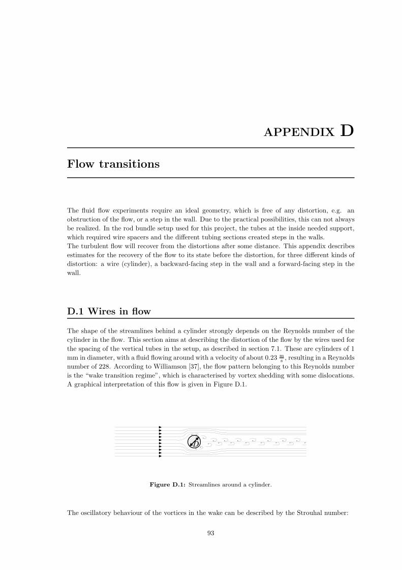
APPENDIX D
Flow transitions
The fluid flow experiments require an ideal geometry, which is free of any distortion, e.g. an
obstruction of the flow, or a step in the wall. Due to the practical possibilities, this can not always
be realized. In the rod bundle setup used for this project, the tubes at the inside needed support,
which required wire spacers and the different tubing sections created steps in the walls.
The turbulent flow will recover from the distortions after some distance. This appendix describes
estimates for the recovery of the flow to its state before the distortion, for three different kinds of
distortion: a wire (cylinder), a backward-facing step in the wall and a forward-facing step in the
wall.
D.1 Wires in flow
The shape of the streamlines behind a cylinder strongly depends on the Reynolds number of the
cylinder in the flow. This section aims at describing the distortion of the flow by the wires used for
the spacing of the vertical tubes in the setup, as described in section 7.1. These are cylinders of 1
mm in diameter, with a fluid flowing around with a velocity of about 0.23 ms , resulting in a Reynolds
number of 228. According to Williamson [37], the flow pattern belonging to this Reynolds number
is the “wake transition regime”, which is characterised by vortex shedding with some dislocations.
A graphical interpretation of this flow is given in Figure D.1.
Figure D.1: Streamlines around a cylinder.
The oscillatory behaviour of the vortices in the wake can be described by the Strouhal number:
93

94 APPENDIX D. FLOW TRANSITIONS
Sr =f L
v(D.1)
with f the frequency, L the length scale and v the velocity of the flow. The value of Sr scales with
the Reynolds number, according the following relation, which is given by Fey et al. [38],
Sr = Sr∗ +m√Re
. (D.2)
The coefficients for the range 180 < Re < 230 are Sr∗ = 0.2437 and m = −0.8607, resulting in a
value for Sr of 0.187. Substitution into Equation D.1, yields a frequency of the vortices of 43 Hz.
The behaviour of the wake directly behind the cylinder has been studied extensively, but the
effects of the wake at a large distance is largely unknown [37]. Two estimates can be made for the
length of the wake, and the accompanying distortion of the flow. The first is given by Williamson
[37], which states that the length of the wake is estimated by
x
D≈ 300 (D.3)
with x the distance to the cylinder and D the diameter. For the 1 mm wires, the wake will have
a length of 0.30 m.
An alternative way is by considering the number of cycles each vortex will make. It can be assumed
that they are neglectable after 100 periods. Using their frequency f = 43 Hz, 100 periods taketf = 100
43 = 2.33 s. The fluid flow of 0.23 m/s brings the vortices over a distance of 0.53 m when
they become negligible.
D.2 Backward-facing step
Fluid flowing over a step in the wall of the channel, cannot flow fully along the wall. The streamlines
will detach from the wall, and at some distance downstream attach again. The situation for a
backward-facing step is depicted in Figure D.2.
Figure D.2: Geometry of the backward-facing step with an indication of the streamlines.
When the flow passes the step, it detaches and the flow will gradually expand in the new room, until
it reattaches again. The time and accompanying distance for this situation, strongly depends on the

D.3. FORWARD-FACING STEP 95
Reynolds number of the flow. Armaly et al. [39] investigated this theoretically and experimentally,
and found a relation for the Reynolds number of the flow in the rod-bundle geometry (Re = 9100)
of:
L
H≈ 7 (D.4)
with L the distance between the step and position of reattachment and H the height of the step.
The fluid flow near the wall is almost laminar, when considering the step height and local fluid
velocity. Considering a step of 1 mm, the fluid velocity is approximately twice as low, which gives
a local Re-number of 1.2 · 102; the flow near the wall behaves as laminar. After reattachment, one
can consider the near-wall flow to be settled again.
D.3 Forward-facing step
The forward-facing step is a sudden narrowing of the flow area. The streamlines have to adjust
themselves to the step, resulting in two vortices, one just before the step and one just downstream,
as drawn in Figure D.3.
A major difference with the backward-facing step is that the forward-facing step also influences
the flow at the upstream side of the step. The vortex downstream of the step has, according to
Ando and Shakouchi [40], a length of:
L
H≈ 1.9. (D.5)
The flow near the wall will behave laminar due to its low velocity, just like with the backward-facing
step. Because the flow area reduces on the step, the main flow will notice this change immediately.
Due to the more abrupt distortion of the flow, more distance is required for a full re-development
of the flow.Tachie et al. [41] suggest that at xH ≈ 50 the mean flow field is recovered, with x the
distance to the step.
Figure D.3: Geometry of the forward-facing step with an indication of the streamlines.

Bibliography
[1] A. Mahmood, M. Rohde, L.M. Portela, T.H.J.J. van der Hagen, and R.F. Mudde. An experi-
mental study of cross flow between two channels connected by a near wall curved gap region.
In Proc. 7th International Topical Meeting on Nuclear Reactor Thermal Hydraulics, Operation
and Safety Seoul, Korea, October 5-9, 2008, 2008.
[2] Axel S. Lexmond, Rob F. Mudde, and Tim H.J.J. van der Hagen. Visualisation of the vortex
street and characterisation of the cross flow in the gap between two sub-channels. In Proc.
11th International Topical Meeting on Nuclear Thermal Hydraulics (NURETH-11) October 2
- 6, number 122, 2005.
[3] T. Ikeno and T. Kajishima. Analysis of dynamical flow structure in a square arrayed rod
bundle. In Proc. 12th International Topical Meeting on Nuclear Reactor Thermal Hydraulics
(NURETH-12) September 30 - October 4, 2007.
[4] Z. Zhang, K. Suzuki, S Hosokawa, and A. Tomiyama. Motion of small bubbles near a grid
spacer in a two by three rod bundle. Journal of Fluid Science and Technology, 3(1):172–182,
2008.
[5] J. Nikuradse. Untersuchungen uber die Geschwindigkeitsverteilung in turbulenten
Stromungen. Forschungsarbeiten auf dem Gebiete des Ingenieurswesens, volume 281, 1926.
[6] L. Prandtl. Uber die ausgebildete Turbulenz. In Verhandlungen des 2. internationalen Kon-
gresses fur technische Mechanik, pages 62–74. Orell Fussli Verlag Zurich und Leipzig, 1927.
[7] R.J. Belt. On the liquid film in inclined annular flow. PhD thesis, Delft University of Tech-
nology, 2007.
[8] E. Brundrett and W.D. Baines. The production and diffusion of vorticity in duct flow. J. of
Fluid Mechanics, 19:375–392, 1964.
[9] A.C.L.M. Daalmans. LDA measurements of particle-driven secondary flow in horizontal an-
nular flow. Master’s thesis, TU Delft, 2005.
[10] P. Bradshaw. Turbulent Secondary Flows. Ann. Rev. Fluid Mech., pages 19: 53–74, 1987.
[11] F.B. Gessner. The origin of secondary flow in turbulent flow along a corner. J. Fluid Mech.,
58:1–25, 1973.
[12] A. Huser and S. Biringen. Direct numerical simulation of turbulent flow in a square duct. J.
Fluid Mech., 1993.
[13] F. Durst, A. Melling, and J. H. Whitelaw. Principles and Practice of Laser-Doppler Anemom-
etry. Academic Press Inc., 1976.
96

BIBLIOGRAPHY 97
[14] M.J. Tummers. Investigation of a turbulent wake in an adverse pressure gradient using Laser
Doppler Anemometry. PhD thesis, Delft University of Technology, 1999.
[15] R.J. Adrian. Fluid mechanics measurements edited by R.J. Goldstein. Springer Berlin, 1983.
chapter V: Laser Velocimetry.
[16] D.K. McLaughlin and W.G. Tiederman. Biasing correction for individual realization of laser
anemometer measurements in turbulent flows. The physics of fluids, 16(12), 1973.
[17] L.H.J. Absil. Analysis of the Laser Doppler Measurement Technique for application in turbu-
lent flows. PhD thesis, Delft University of Technology, 1995.
[18] A. Nakayama. Measurements of seperating Boundary Layer and Wake of an Airfoil using
Laser Doppler Velocimetry. AIAA paper 0181, 23rd Aerospace Sciences Meeting, 1985.
[19] R. V. Edwards, A. Dybbs, R. Adrian, A. Boutier, J. Eaton, W. George, and J. Meyers.
Report of the Special Panel on statistical particle bias problems in laser anemometry. ASME
Transactions Journal of Fluids Engineering, 109:89–93, June 1987.
[20] W.T. Mayo, M.T. Shay, and S. Riter. Digital Estimation of Turbulence Power Spectra from
Burst counter LDV data. In Proceedings of the second international workshop on laser ve-
locimetry, Volume I., pages 16–26. Texas A&M University College Station, Texas, 1974.
[21] H. Nobach, E. Muller, and C. Tropea. Refined reconstruction techniques for LDA data anal-
ysis. In Proceedings of the 8th International Symposium of Applications of laser techniques to
fluid mechanics, number paper 36.2. Instituto Superior Tecnico, Lisbon, Portugal, 1996.
[22] E. Muller, H. Nobach, and C. Tropea. A refined reconstruction-based correlation estima-
tor for two-channel, non-coincidence laser Doppler anemometry. Measurement Science and
Technology, 9:442–451, March 1998.
[23] L. H. Benedict, H. Nobach, and C. Tropea. Estimation of turbulent velocity spectra from
laser Doppler data. Measurement Science and Technology, 11:1089–1104, August 2000.
[24] M. J. Tummers and D. M. Passchier. Rapid Communication: Spectral estimation using a
variable window and the slotting technique with local normalization . Measurement Science
and Technology, 7:1541–1546, November 1996.
[25] H. Nobach, E. Muller, and C. Tropea. Correlation estimator for two-channel, non-coincidence
laser-doppler-anemometer. In Proceedings of the 9th International Symposium of Applica-
tions of laser techniques to fluid mechanics, number paper 32.1. Instituto Superior T/’ecnico,
Lisbon, Portugal, 1998.
[26] H. Nobach. Processing of stochastic sampled data in Laser Doppler Anemometry. In Proceeding
of the 3rd International Workshop on Sampling theory and applications, pages 149–154. Dantec
Measurement Technology A/S, Denmark, Norwegian University of Science and Technology,
Trondheim, 1999.
[27] H. Nobach. Local time estimation for the slotted correlation function of randomly sampled
LDA data. Experiments in Fluids, 32:337–345, 2002.
[28] H. R. E. van Maanen and A. Oldenziel. Estimation of turbulence power spectra from ran-
domly sampled data by curve-fit to the autocorrelation function applied to laser-Doppler
anemometry. Measurement Science and Technology, 9:458–467, March 1998.
98 BIBLIOGRAPHY
[29] R. Budwig. Refractive index matching methods for liquid flow investigations. Experiments in
fluids, 17(5):350–355, September 1994.
[30] J.G.M. Eggels, F. Unger, M.H. Weiss, J. Westerweel, R.J. Adrian, R. Friedrich, and F.T.M.
Nieuwstadt. Fully developed turbulent pipe flow: A comparison between direct numerical
simulation and experiment. J. Fluid Mech., 268:175–209, 1994.
[31] J.M.J. den Toonder. Drag reduction by polymer additives in a turbulent pipe flow: laboratory
and numerical results. PhD thesis, Delft University of Technology, 1995.
[32] Tsutomu Ikeno and Takeo Kajishima. Analysis of dynamical flow structure in a square arrayed
rod bundle. Nuclear Engineering and Design, In Press, Corrected Proof:–, 2008. ISSN 0029-
5493.
[33] A. Cenedese, G.P. Romano, and F.D. Felice. Experimental testing of Taylor’s hypothesis by
L.D.A. in highly turbulent flow. Experiments in fluids, 11:351–358, 1991.
[34] H Tennekes and J.L. Lumley. A first course in Turbulence. The MIT Press, 1972.
[35] P.A. Davidson. Turbulence, an introduction for scientists and engineers. Oxford University
Press, 2004.
[36] Adtech Polymer Engineering. Technical data of adtech fluoroplastic polymers. Technical
report, DuPont, 2008. Accessible via website: http://www.adtech.co.uk/.
[37] C.H.K. Williamson. Vortex dynamics in the cylinder wake. Annual Reviews Fluid Mechanics,
pages 28:477–539, 1996.
[38] Uwe Fey, Michael Konig, and Helmut Eckelmann. A new strouhal–reynolds-number relation-
ship for the circular cylinder in the range 47 < Re < 2·105. Physics of Fluids, 10(7):1547–1549,
1998.
[39] B. F. Armaly, F. Durst, J. C. F. Pereira, and B. Schonung. Experimental and theoretical
investigation of backward-facing step flow. Journal of Fluid Mechanics, 127:473–496, 1983.
[40] T. Ando and T. Shakouchi. Flow characteristics over forward facing step and through abrupt
contraction pipe and drag reduction. Research Reports of the faculting of Engineering, Meiji
University, vol. 29:1–8, 2004.
[41] Mark F. Tachie, Ram Balachandar, and D. J. Bergstrom. Open channel boundary layer relax-
ation behind a forward facing step at low reynolds numbers. Journal of Fluids Engineering,
123(3):539–544, 2001.