noise modeling in universiti sains malaysia and offshore

NOISE MODELING IN UNIVERSITI SAINS MALAYSIA AND OFFSHORE OIL AND GAS PLATFORM

HANG SEE PHENG

UNIVERSITI SAINS MALAYSIA

2007


by

HANG SEE PHENG

Thesis submitted in fulfillment of the requirements for the degree

of Master of Science

November 2007

ii

ACKNOWLEDGEMENTS

First of all, I would like to express my deepest gratitude to my main

supervisor, Professor Koh Hock Lye for his guidance and dedication towards

the completion of my thesis. I would like to extend my sincere appreciation to

my co-supervisor, Puan Suraiya Kassim for her assistance and advice in

achieving the objective of this thesis.

In addition, I would like to thank the Graduate Assistance Scheme (GAS)

for financial support in my studies. Further, I am grateful to the School of

Mathematical Sciences, School of Housing Building and Planning, the Institute

of Post Graduates Studies as well as libraries of USM for providing various

facilities and references. Last but at least, I would like to thank my family for

their great moral support and to my friends for their contributions in completing

my thesis.

iii

TABLE OF CONTENTS

Page

ACKNOWLEDGEMENTS ii

TABLE OF CONTENTS iii

LIST OF TABLES viii

LIST OF FIGURES x

LIST OF SYMBOLS xii

LIST OF ABBREVIATION xvi

ABSTRAK xvii

ABSTRACT xix

CHAPTER 1: INTRODUCTION

1

1.1 Introduction to Noise Pollution Modeling 1

1.2 New Science Complex (NSC) 3

1.3 Jalan Sungai Dua 3

1.4 Offshore Oil and Gas Platform 4

1.5 Problem Statement and Objectives of Thesis 5

1.6 Scope and Organization of Thesis 5

CHAPTER 2: LITERATURE REVIEW

9

2.1 Introduction 9

2.2 Noise Models and Related Studies 10

2.3 Traffic Noise Simulation Model 13

2.3.1 FHWA Traffic Noise Model 15

2.3.2 Other Traffic Noise Models 18

2.4 Noise Control Barriers 24

iv

CHAPTER 3: MODELING NOISE LEVELS IN NEW SCIENCE COMPLEX

26

3.1 Introduction 26

3.2 Standards and Criteria of Noise 27

3.3 Acoustical Characteristics and Levels 29

3.3.1 Frequency 30

3.3.2 Sound Power Level 30

3.3.3 Sound Pressure Level 31

3.3.4 Addition of Sound Pressure Level 31

3.3.5 Average of Sound Pressure Level 32

3.4 Sound Propagation 32

3.4.1 Point Source in Free Field Propagation 32

3.4.2 Sound Absorption 34

3.4.3 Sound Reflection 35

3.4.4 Sound Transmission 36

3.5 New Science Complex (NSC) 38

3.6 Field Survey 39

3.6.1 Data Collection 40

3.6.2 Social Survey 41

3.7 NOISEPAC Simulation for NSC 44

3.8 Result of NOISEPAC Simulation 45

3.8.1 Statistical Analysis 47

3.8.2 Discussion 49

3.9 Noise Control 51

3.10 Conclusion 53

v

CHAPTER 4: MODELING TRAFFIC NOISE LEVELS AROUND USM PENANG

54

4.1 Introduction 54

4.2 Traffic Noise Model version 2.5 (TNM 2.5) 56

4.2.1 Vehicle Noise Emissions 58

4.2.2 Vehicle Speed Computation 59

4.2.3 Horizontal Geometry and Acoustics 60

4.2.3.1 Traffic Flow Adjustments 61

4.2.3.2 Distance and Roadway Length Adjustment 62

4.2.4 Vertical Geometry and Acoustics 63

4.3 Study Area 65

4.3.1 Data and Field Survey 66

4.4 TNM 2.5 Input 68

4.5 Results and Discussion 70

4.5.1 Statistical Analysis 72

4.5.2 Traffic Noise Impact 75

4.6 Traffic Noise Mitigation 76

4.6.1 TNM 2.5 Barrier Analysis 77

4.6.1 Proposed Barrier in Study Area 78

4.7 Conclusion 80

CHAPTER 5: MODELING NOISE LEVELS ON OFFSHORE OIL AND GAS PLATFORM

82

5.1 Introduction 82

5.2 The Occupational Noise Regulations 83

5.2.1 “First Schedule” in Permissible Exposure Limits (PEL) 84

5.2.2 Noise Exposure Dose (NED) 85

5.3 Noise Surveys on Offshore Oil and Gas Platform 86

5.3.1 Esso Production Malaysia Incorporated (EPMI) 86

5.4 Offshore Oil and Gas Platform 88

5.4.1 Noise Sources 91

vi

5.5 NOISEPAC 93

5.5.1 Input Sound Levels 94

5.5.2 Sound Reflection and Transmission 94

5.6 Predicted Noise Levels 96

5.6.1 WHRU and Coolers Deck 96

5.6.1.1 Scenario A 97

5.6.1.2 Scenario B 98

5.6.2 Production Deck 99



5.6.3 Mezzanine Deck 101



5.6.4 Cellar Deck 103



5.6.5 Discussion 105

5.7 Offshore Industry Noise Control 107

5.8 Conclusion 109

CHAPTER 6: CONCLUSION AND RECOMMENDATION

110

REFERENCES

114

APPENDICES

Appendix A Air-Conditioning System in New Science Complex 122

Appendix B Data Collection in New Science Complex (NSC) 123

Appendix C Social Survey in New Science Complex (NSC) 129

Appendix D NOISEPAC Program 130

Appendix E Input File in NOISEPAC 143

vii

Appendix F Noise Contour in New Science Complex (NSC) 145

Appendix G Picture of Field Survey for Traffic Noise Monitoring 159

Appendix H Data Collection for Traffic Noise Monitoring 161

Appendix I Input Data in TNM 2.5 168

Appendix J Output Data in TNM 2.5 173

Appendix K Noise Labeling in Industry Area 174

LIST OF PUBLICATIONS 175

viii

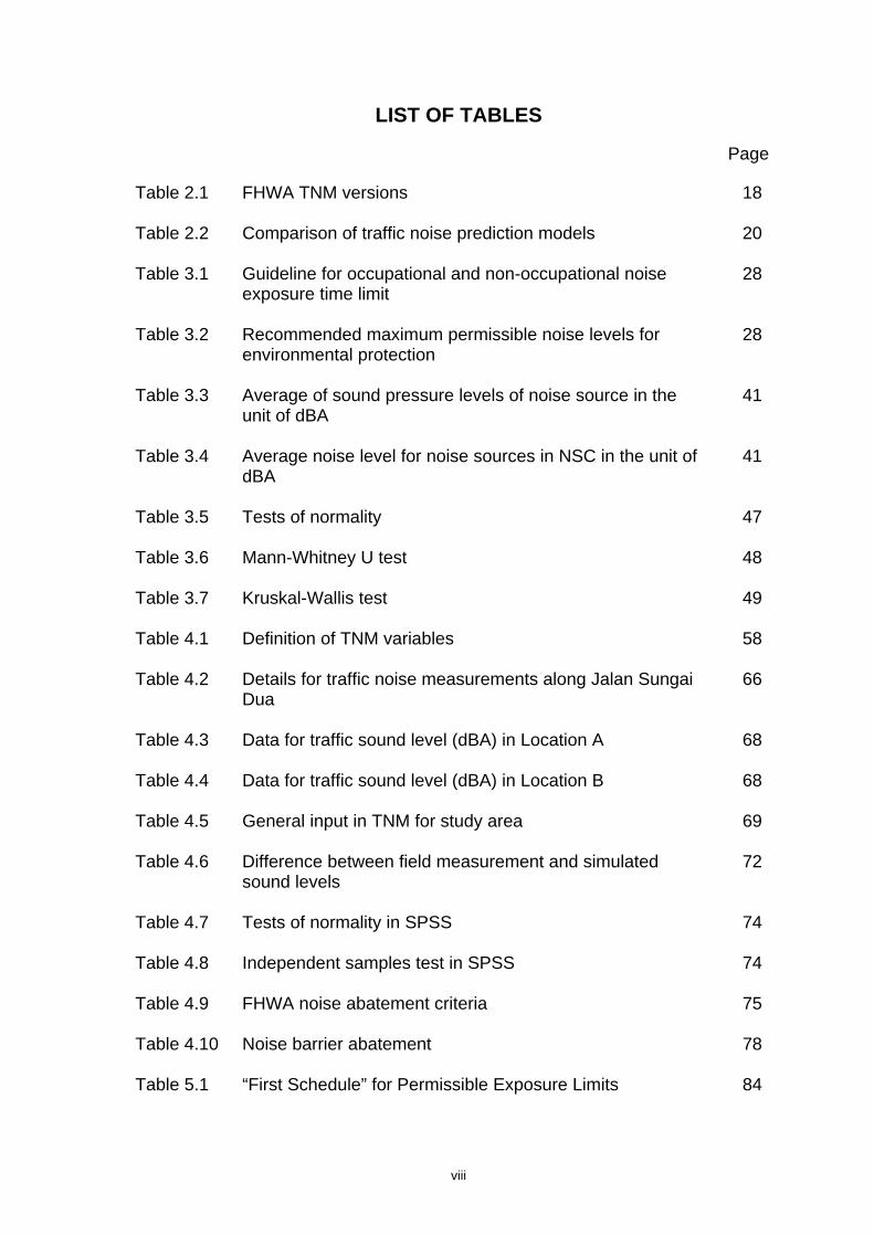
LIST OF TABLES

Page

Table 2.1 FHWA TNM versions

18

Table 2.2 Comparison of traffic noise prediction models

20

Table 3.1 Guideline for occupational and non-occupational noise exposure time limit

28

Table 3.2 Recommended maximum permissible noise levels for environmental protection

28

Table 3.3 Average of sound pressure levels of noise source in the unit of dBA

41

Table 3.4 Average noise level for noise sources in NSC in the unit of dBA

41

Table 3.5 Tests of normality

47

Table 3.6 Mann-Whitney U test

48

Table 3.7 Kruskal-Wallis test

49

Table 4.1 Definition of TNM variables

58

Table 4.2 Details for traffic noise measurements along Jalan Sungai Dua

66

Table 4.3 Data for traffic sound level (dBA) in Location A

68

Table 4.4 Data for traffic sound level (dBA) in Location B

68

Table 4.5 General input in TNM for study area

69

Table 4.6 Difference between field measurement and simulated sound levels

72

Table 4.7 Tests of normality in SPSS

74

Table 4.8 Independent samples test in SPSS

74

Table 4.9 FHWA noise abatement criteria

75

Table 4.10 Noise barrier abatement

78

Table 5.1 “First Schedule” for Permissible Exposure Limits

84

ix

Table 5.2 Typical noise sources on oil and gas platform

92

Table 5.3 Typical noise levels at 1 meter on offshore structure without specific noise control measures

93

Table 5.4 Input parameters on WHRU and coolers deck

97

Table 5.5 Input parameters on production deck

99

Table 5.6 Input parameters on mezzanine deck

101

Table 5.7 Input parameters on cellar deck

103

Table 5.8 Basic noise control measures on offshore installations

108

x

LIST OF FIGURES

Page

Figure 3.1 Typical sound levels in sound pressure level (decibels) and psi for several conditions

30

Figure 3.2 Plan for study area and the locations of data collection

39

Figure 3.3 Percentage of the degree of noise condition

42

Figure 3.4 Percentage of psychology effect caused by air-conditioning system

43

Figure 3.5 Comparison of measured data and NOISEPAC simulated results

46

Figure 3.6 Noise contours of sound field for seven levels of the NSC

50

Figure 3.7 Multiple-edge of noise control barriers

52

Figure 4.1 Initial element triangle

60

Figure 4.2 Maximum elemental triangle set to 10 degrees

60

Figure 4.3 Definition of relevant distances and angles

63

Figure 4.4 Study Area and Data Collection Locations (Location A an B)

65

Figure 4.5 Percentage of each vehicle type in Jalan Sg Dua

67

Figure 4.6 Comparison of measured and TNM simulated results at Location A

71

Figure 4.7 Comparison of measured and TNM simulated results at Location B

71

Figure 4.8 Noise analysis contour along Jalan Sungai Dua

76

Figure 4.9 Optimal angle of view for an effective noise control barrier

78

Figure 4.10 Proposed Barrier in study area

79

Figure 4.11 Noise reduction contour

80

Figure 5.1 Plan views for vertical structure of the design platform

90

Figure 5.2 Noise contour on WHRU and coolers deck (scenario A)

98

xi

Figure 5.3 Noise contour on WHRU and coolers deck (scenario B)

98

Figure 5.4 Noise contour for production deck (scenario A)

100

Figure 5.5 Noise contour for production deck (scenario B)

101

Figure 5.6 Noise contour on mezzanine deck (scenario A)

102

Figure 5.7 Noise contour on mezzanine deck (scenario B)

103

Figure 5.8 Noise contour on cellar deck (scenario A)

104

Figure 5.9 Noise contour on cellar deck (scenario B)

105

xii

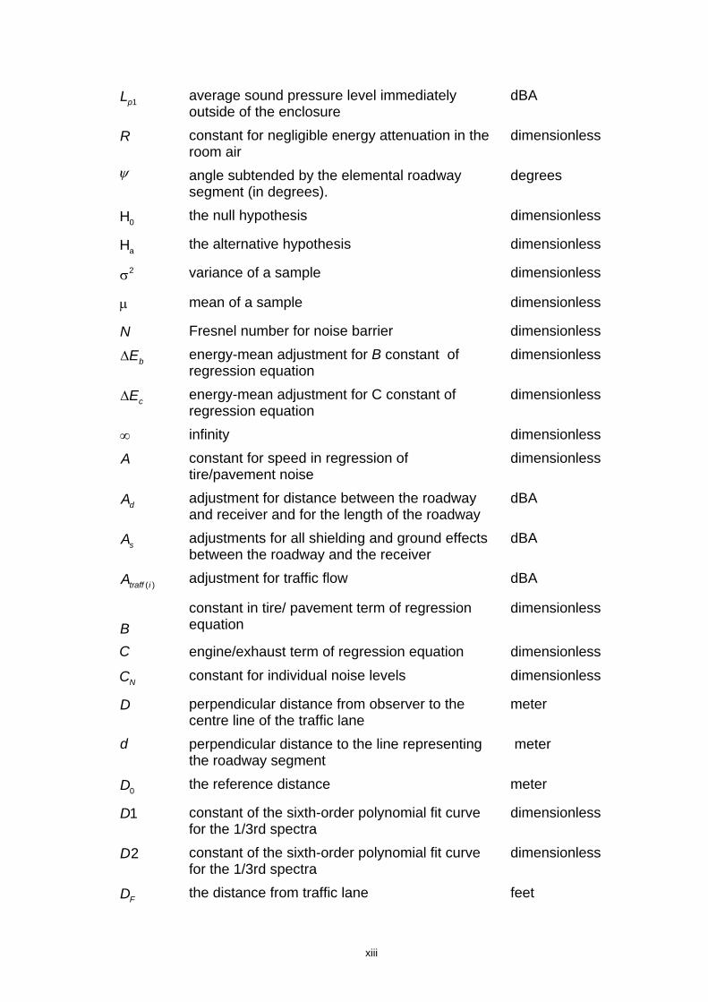
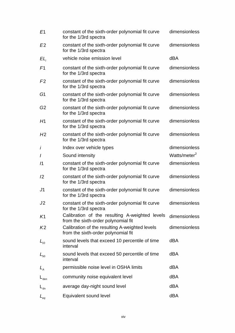
LIST OF SYMBOLS

Symbols Descriptions Units

f nominal 1/3rd-octave-band center frequency Hertz

is vehicle speed kilometer/hour

(1 h)AeqL equivalent sound level over one hour time period dBA

β ground effect adjustment dimensionless

W sound power Watts

refW reference sound power Watts

absW acoustic energy absorbed by the surface Watts

inW acoustic energy striking the surface Watts

p root-mean-square(rms) sound pressure Pascal

refp reference sound pressure Pascal

π the ratio of the circumference to the diameter of a circle (given 3.14159)

dimensionless

Q ratio of the intensity on a designated axis of a sound radiator

dimensionless

ρc characteristics impedance of medium mks rayls

DI directivity index dimensionless

r radial distance of receiver from the source meter α sound absorption coefficient dimensionless

α j absorption coefficient of the j th surface dimensionless

τ sound transmission coefficient. dimensionless

jS surface area of the j th surface meter2

oS total surface area of the room meter2

wS surface area of external walls meter2

,p imageL sound pressure levels from image source dBA

,w imageL sound power level of image source dBA

,w originalL sound power levels of original source dBA

,w wallL sound power transmission level into the enclosure through external walls of surface area

dBA

xiii

1pL average sound pressure level immediately outside of the enclosure

dBA

R constant for negligible energy attenuation in the room air

dimensionless

ψ angle subtended by the elemental roadway segment (in degrees).

degrees

0H the null hypothesis dimensionless

aH the alternative hypothesis dimensionless

σ2 variance of a sample dimensionless

μ mean of a sample dimensionless

N Fresnel number for noise barrier dimensionless

Δ bE energy-mean adjustment for B constant of regression equation

dimensionless

Δ cE energy-mean adjustment for C constant of regression equation

dimensionless

∞ infinity dimensionless

A constant for speed in regression of tire/pavement noise

dimensionless

dA adjustment for distance between the roadway and receiver and for the length of the roadway

dBA

sA adjustments for all shielding and ground effects between the roadway and the receiver

dBA

( )traff iA adjustment for traffic flow dBA

B

constant in tire/ pavement term of regression equation

dimensionless

C engine/exhaust term of regression equation dimensionless

NC constant for individual noise levels dimensionless

D perpendicular distance from observer to the centre line of the traffic lane

meter

d perpendicular distance to the line representing the roadway segment

meter

0D the reference distance meter

1D constant of the sixth-order polynomial fit curve for the 1/3rd spectra

dimensionless

2D constant of the sixth-order polynomial fit curve for the 1/3rd spectra

dimensionless

FD the distance from traffic lane feet

xiv

1E constant of the sixth-order polynomial fit curve for the 1/3rd spectra

dimensionless

2E constant of the sixth-order polynomial fit curve for the 1/3rd spectra

dimensionless

iEL vehicle noise emission level dBA

1F constant of the sixth-order polynomial fit curve for the 1/3rd spectra

dimensionless

2F constant of the sixth-order polynomial fit curve for the 1/3rd spectra

dimensionless

1G constant of the sixth-order polynomial fit curve for the 1/3rd spectra

dimensionless

2G constant of the sixth-order polynomial fit curve for the 1/3rd spectra

dimensionless

1H constant of the sixth-order polynomial fit curve for the 1/3rd spectra

dimensionless

2H constant of the sixth-order polynomial fit curve for the 1/3rd spectra

dimensionless

i Index over vehicle types dimensionless

I Sound intensity Watts/meter2

1I constant of the sixth-order polynomial fit curve for the 1/3rd spectra

dimensionless

2I constant of the sixth-order polynomial fit curve for the 1/3rd spectra

dimensionless

1J constant of the sixth-order polynomial fit curve for the 1/3rd spectra

dimensionless

2J constant of the sixth-order polynomial fit curve for the 1/3rd spectra

dimensionless

1K Calibration of the resulting A-weighted levels from the sixth-order polynomial fit

dimensionless

2K Calibration of the resulting A-weighted levels from the sixth-order polynomial fit

dimensionless

10L sound levels that exceed 10 percentile of time interval

dBA

50L sound levels that exceed 50 percentile of time interval

dBA

AL permissible noise level in OSHA limits dBA

denL community noise equivalent level dBA

dnL average day-night sound level dBA

eqL Equivalent sound level dBA

xv

(10 )eqL s equivalent sound level in 10 seconds dBA

pL sound pressure level dBA

,p totalL summation of sound pressure levels dBA

NL all sound levels sets in the prediction model dBA

trafL traffic sound level dBA

wL sound power level dBA

n number of each type vehicles per hour dimensionless

p Index over pavements types dimensionless

HP percentage of heavy trucks percent

S mean vehicle speed miles/hour

TL sound transmission loss dBA

V traffic volume vehicles/hour C time of exposure to a noise level hours/day IL insertion loss dBA T total permitted exposure times at a noise level hours/day

xvi

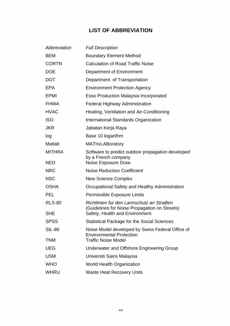
LIST OF ABBREVIATION

Abbreviation Full Description

BEM Boundary Element Method

CORTN Calculation of Road Traffic Noise

DOE Department of Environment

DOT Department of Transportation

EPA Environment Protection Agency

EPMI Esso Production Malaysia Incorporated

FHWA Federal Highway Administration

HVAC Heating, Ventilation and Air-Conditioning

ISO International Standards Organization

JKR Jabatan Kerja Raya

log Base 10 logarithm

Matlab MATrixLABoratory

MITHRA Software to predict outdoor propagation developed by a French company

NED Noise Exposure Dose

NRC Noise Reduction Coefficient

NSC New Science Complex

OSHA Occupational Safety and Healthy Administration

PEL Permissible Exposure Limits

RLS-90 Richtlinien fur den Larmschutz an StraBen (Guidelines for Noise Propagation on Streets)

SHE Safety, Health and Environment

SPSS Statistical Package for the Social Sciences

StL-86 Noise Model developed by Swiss Federal Office of Environmental Protection

TNM Traffic Noise Model

UEG Underwater and Offshore Engineering Group

USM Universiti Sains Malaysia

WHO World Health Organization

WHRU Waste Heat Recovery Units

xvii

PEMODELAN BUNYI BISING DI UNIVERSITI SAINS MALAYSIA DAN PELANTAR MINYAK DAN GAS LEPAS PANTAI

ABSTRAK

Dalam beberapa dekad lepas, pencemaran bunyi bising telah meningkat

secara berterusan disebabkan oleh perkembangan perbandaran dan

perindustrian yang pesat. Ia telah dikategorikan sebagai salah satu masalah

utama alam sekitar dan juga dikaitkan dengan isu-isu bagi kesihatan fizikal dan

mental. Oleh itu, beberapa undang-undang mengenai bunyi bising telah

dikuatkuasakan di beberapa negara untuk memastikan objektif kesihatan orang

ramai and alam sekitar tercapai. Tesis ini akan membentangkan permodelan

bunyi bising dengan menggunakan model NOISEPAC dan model bunyi bisng

trafik, versi 2.5 (TNM 2.5). Satu penyelidikan telah dimulakan untuk memantau

dan memodelkan dengan menggunakan NOISEPAC tahap bunyi bising di

Universiti Sains Malaysia, di mana staf and pelajar di Kompleks Sains Baru

(NSC) telah menghadapi gangguan bunyi bising yang disebabkan oleh bunyi

yang disebarkan oleh system penghawa dingin. Selain itu, TNM 2.5 telah

digunakan untuk mengkaji tahap bunyi bising trafik di sekitar Jalan Sungai Dua,

iaitu sebatang jalan raya sibuk yang berdekatan dengan kampus utama USM.

Tinjauan lapangan dilakukan di sekitar NSC dan kampus USM untuk

memperolehi data pengesahan dan parameter masukan dalam implementasi

kedua-dua model peramalan. Selanjutnya, NOISEPAC diubahsuai untuk

mengkaji tahap bunyi bising di pelantar minyak dan gas lepas pantai. Tahap

bunyi bising di atas struktur lepas pantai dijangka tinggi disebabkan oleh

kepadatan modul berstruktur keluli dengan berbagai-bagai punca bunyi bising.

Model peramalan bunyi bising adalah satu alat untuk menilai bunyi bising alam

xviii

sekitar pada tahap rekaan dan keadaan semasa. Ia juga perlu untuk

penyediaan dasar dalam pemilihan langkah peringanan bunyi bising.

xix


ABSTRACT

Over the last few decades, noise pollution has steadily increased due to

rapid urbanization and industrialization. It has been categorized as a major

environmental problem as well as being related to physical and mental health

issues. Hence, several noise regulations have been implemented in various

countries to ensure that broad public health and environmental objectives are

met. This thesis will present modeling of noise levels using an in-house noise

model, NOISEPAC and Traffic Noise Model version 2.5 (TNM 2.5). A research

is initiated to monitor and model, by means of NOISEPAC, noise levels in

Universiti Sains Malaysia (USM), where staffs and students in the New Science

Complex (NSC) have experienced some noise annoyance due to the sound

emitted from air-conditioning system. Apart from that, TNM 2.5 is used to

analyze traffic noise levels around Jalan Sungai Dua, a busy roadway located

near the USM main campus. Field surveys are conducted around the NSC and

USM campus in order to obtain validation data and input parameters for the

implementation of both prediction models. Further, NOISEPAC is modified to

analyze noise levels on an offshore oil and gas platform. Noise levels on an

offshore structure are expected to be high due to the compact steel structure

modules with multiple noise sources. Noise prediction models are tools to

assess the environment noise in the design and existing stage. They are also

essential to provide a basis for the selection of noise mitigation measures.

1

CHAPTER 1

INTRODUCTION

1.1 Introduction to Noise Pollution Modeling

In recent decades, noise pollution has increased due to the rapid

urbanization and industrialization, especially in the developing countries. Some

common noise that exists in the environment include machinery noise,

transportation noise, construction noise, public works noise, building services

noise and noise from leisure activities. According to the Occupational Safety

and Healthy Administration (OSHA), exposure to high levels of noise for long

durations may lead to hearing loss, create physical and psychological stress,

reduce productivity and interfere with communication (OSHA, 2006). The main

social consequence of hearing impairment is the incapability to understand

speech in normal environment, which is considered as a social handicap (WHO,

2006). Hence, it is important that environmental sound level be maintained at a

safe and comfortable condition. However, sound that is classified as noise, such

as the warning whistle from a train, is actually beneficial for it acts as a warning

for people during a potential dangerous situation (Barron, 2003).

Several major federal agencies in USA, such as the Occupational Safety

and Healthy Administration (OSHA), the Environment Protection Agency (EPA),

the Federal Highway Administration (FHWA) have adopted noise policies and

standards to regulate noise levels. The policy guidelines are used as a basis to

ensure that the broad public health and environment objectives are met. In

Malaysia, noise regulation is set by Department of Environment (DOE) under

2

the Environment Quality Act, 1974 (DOE, 2007). As a practical measure, the

selection of locations and designs for urban buildings is important to avoid

excessive noise levels. It is more cost effective to implement noise control at the

design stage. For existing building and facilities, noise levels can be controlled

by using noise control measures such as enclosures, absorbers, silencers and

personal protective equipments, such as earmuffs. However, controlling noise at

the source is usually recognized as the most effective solution in noise control

problems (Bies, 2003). The controls of noise at the source may involve

maintenance and substitution of equipments and machines.

Currently, several noise analysis models have been developed to predict

sound pressure levels and to assess mitigation measures. These noise models

have become an important and cost effective tool to design a better working

and living environment. This thesis will focus on the modeling of noise levels in

the Universiti Sains Malaysia (USM), Penang campus including the adjacent

road and a typical oil and gas platform. Under the Healthy Campus Program,

which strives for a better campus environment, a research program is

conducted to assess the noise level emitted by the air conditioning systems in

the New Science Complex (NSC) in USM. An in-house noise simulation model,

NOISEPAC is developed based upon mathematical and acoustical principles to

simulate noise levels in the vicinity of the NSC (Hang et al., 2006). This thesis

will also analyze the impact of traffic noise levels on USM compound by using

the Federal Highway Administration Traffic Noise Model, version 2.5 (TNM 2.5).

The effectiveness of the TNM 2.5 barrier analysis in reducing the traffic noise

levels along the roadway will be presented. Finally, this thesis will present noise

3

modeling analysis on an offshore oil and gas platform with complicated

alignment of production facilities. The research on offshore platform noise levels

will be performed by means of the modified NOISEPAC model simulations.

1.2 New Science Complex (NSC)

The New Science Complex (NSC) was completed in early 2000 to

accommodate staffs and students of the School of Computer Sciences and the

School of Mathematical Sciences. An air conditioning system known as the “Air

Cooled Rotary Screw Flooded Chillers” was installed to provide comfortable

environment to the staffs and students in the building. Within the compound of

the NSC, the air conditioning system was located at about 3.5 meters above

ground level. Staffs working in the NSC have experienced some noise

annoyance due to sound emanating from the air-condition exhausts. A concern

is raised as to whether the noise level produced by the air conditioning system

will pose hazards to the staffs and students who work in the NSC for long

duration. For the purpose of assessing noise level in NSC, a field survey has

been conducted in the surrounding area of the building. An in-house noise

simulation model NOISEPAC is then used to simulate the overall sound field in

the NSC.

1.3 Jalan Sungai Dua

Since the British colonial period, Jalan Sungai Dua is used as a main

roadway by residents that live in Gelugor, Penang. The roadway consists of two

traffic lanes. Rapid development in the Sungai Dua area transforms it from a

rural to an urban environment, resulting a high density of vehicles along this

4

roadway. The traffic noise may create high degree of environmental noise

impact for the surrounding area, due to the high traffic volume and speed

(Tansatcha et al.,2005). Therefore, traffic noise monitoring is conducted to

assess whether the traffic noise level would pose health hazards to the

occupants of adjacent buildings in the USM Campus, Penang. A computer

noise simulation model TNM 2.5 is used to analyze traffic noise impact along

Jalan Sungai Dua.

1.4 Offshore Oil and Gas Platform

Safety, health and environment (SHE) are always the primary concerns

for the oil and gas industry. Confined within a small space, the design of

integrated oil and gas platform is usually complicated by the combination of

production facilities as well as living quarters located close to each other. The

offshore oil and gas platform is commonly used to explore and process crude oil

and gas located in the deep ocean. At the design stage, noise is one of the

factors that may affect the decision of design engineers in the selection of

instruments and their layout on an offshore oil and gas platform to minimize

noise hazards. Due to the long duration of exposure to noise on offshore oil and

gas platform, high noise level in the workplace may cause hearing loss and

damage to the workers. In our research, significant noise sources are identified

and their propagation on the oil and gas platform is predicted by means of the

modified NOISEPAC.

5

1.5 Problem Statement and Objectives of Thesis

The problem statement and objectives for this study are as follows:

1. To model and analyze noise levels in the NSC in USM using an in-

house model NOISEPAC under the current conditions;

2. To model and analyze traffic noise levels around USM, Penang

campus using Traffic Noise Model version 2.5 (TNM, 2.5);

3. To implement the modified NOISEPAC in predicting the

propagation of noise levels on an offshore oil and gas platform;

4. To study noise regulations and noise mitigation methods for

reducing noise levels.

1.6 Scope and Organization of Thesis

This thesis is divided into six chapters. Chapter 1 will briefly discuss the

overall theme of the thesis and present the study sites, objectives, scope and

organization. Chapter 2 will provide a brief description on the literature and

scientific papers that are relevant to noise simulation models. This chapter

begins with a brief introduction to noise simulation modeling and analysis in

industrial areas. Development of traffic noise models since 1950 is also

presented, including the well known traffic noise model TNM, which is

developed by the Federal Highway Administration (FHWA) of USA for predicting

noise levels in the vicinity of highways and for designing highway noise barriers.

Further, comparison between some current traffic noise models such as

CORTN, RLS-90, MITHRA, StL-86 and ASJ Method 1993 are reviewed.

Various noise control barriers that are recognized as popular mitigation

measures will also be discussed in this chapter.

6

Chapter 3 begins with a brief introduction to noise pollution for the air-

conditioning system. The standards of noise and typical sound levels for several

conditions are discussed. An in-house noise prediction model NOISEPAC,

which is programmed in FORTRAN language, is developed to simulate the

overall sound fields in the NSC. This model is built based upon some

mathematical and acoustical formulations typically used. Noise data collection

and social survey in NSC will be presented in this chapter. The overall

measured data compares well with simulated noise levels, indicating proper

performance of NOISEPAC. Further, statistical analysis using the SPSS

statistical software package is then performed to assess accuracy of the

simulation. Using a graphical package Matlab 6.5, noise contours are plotted to

visualize sound fields within the building. By means of the noise contours, we

can easily identify noise-sensitive areas. Several noise mitigation methods will

be suggested for reducing excessive noise levels.

Chapter 4 begins with a broad overview of traffic noise pollution and the

legislation for controlling traffic noise limits. This chapter will focus on traffic

noise analysis using a mathematical software TNM 2.5. Following many years

of upgrades, this model is developed by the Federal Highway Administration in

United States. Several modeling components and formulations in TNM 2.5 will

be discussed. For the purpose of validating the simulated results, data and field

survey in the study site is conducted and then presented in the chapter. Sound

levels from traffic noise along the Sungai Dua roadway are collected and traffic

volumes for different vehicle types are obtained simultaneously. Besides that,

traffic composition and traffic volumes as part of the input parameter in the

7

computer program are also presented. By means of TNM 2.5, the overall traffic

noise levels are simulated for selected areas in USM campus, which are located

near to Jalan Sungai Dua. Then, statistical analysis using the SPSS statistical

package is done to assess model performance by considering the difference

between TNM 2.5 simulated results and measured results. Further, noise level

contour and barrier analysis at the study site will be included in this chapter.

The FHWA noise criteria are compared to the traffic noise levels in the vicinity of

USM campus.

Noise prediction on a typical oil and gas platform is performed in Chapter

5 by using NOISEPAC. The objective of the study in this chapter is to assess

the in-house model NOISEPAC as an analysis tool for potential noise problems

on oil and gas platforms, especially at the early stage of the design of the

platform. This chapter begins with a literature review regarding noise survey in

the oil and gas industry. Several noise standards in Malaysia and other regional

regulation for workplace are studied. We then discuss the layout design and

allocation of equipments that may generate significant noise level. Based upon

the actual sound power level data, which is available in some previous research

studies, the overall noise levels on offshore platform are simulated by using

NOISEPAC. Some theoretical concepts on sound propagation in modeling

noise levels on the offshore oil and gas platform will be also included. Noise

contours generated by Matlab 6.5 will provide a visual image of sound fields on

the platform. Furthermore, some noise control devices available for mitigation

will be discussed in this chapter.

8

Conclusion and further research relevant to the theme of the thesis are

discussed in Chapter 6. We hope that the noise analysis performed in this

thesis will contribute towards the designing of a more friendly environment in

USM and industry workplaces in the future.

9

CHAPTER 2

LITERATURE REVIEW

2.1 Introduction

Generally, noise models are designed to estimate noise levels in urban

areas and working places. The models can be used to assess the degree of

exposure to noise for a given or projected road, highway, railway, airport,

factory or any town planning capable of generating noise annoyance (Garcia,

2001). Most of the noise models assume that noise emitted from a source

attenuate logarithmically with distance away from the noise source (El-Fadel et

al., 2002). With the help of computer graphic programs, the predicted noise

levels can be presented by a noise map for the whole selected area.

This thesis focuses on modeling noise levels in and around the Universiti

Sains Malaysia (USM) main campus in Minden and on offshore oil and gas

production platforms. This chapter contains three sections. Section 2.2 will

briefly review the methods that are used to predict the noise levels in industrial

areas. Section 2.3 will present a review of models to simulate traffic noise levels.

Lastly, Section 2.4 is a review for noise control barriers. An in-house noise

model namely NOISEPAC (Hang et al., 2006) and Federal Highway

Administration Traffic Noise Model (FHWA TNM) version 2.5 (Lau, 2004) are

used in this thesis.

10

2.2 Noise Models and Related Studies

Based upon the diffused-field theory, Abdullah and Mohd Nor (2001)

developed an adaptive 3D Gauss-Legendre Quadrature method. This technique

is used to simulate the propagation of outdoor noise from sources with variable

shapes and power distribution. The advantage of the method is that it takes into

account the geometry of the defined sound sources and produces the

appropriate contours conforming to the shape of the sources. The noise

sources are modeled as an array of point sources which are in the form of lines,

planes and 3D blocks. They recommend that curvy highway or railway

interchanges be modeled as curvy line sources while process plant equipments

and power station buildings should be treated as an array of 3D prism blocks.

This method is suitable for noise levels modeling of large sound sources such

as power plants or highways. The mathematical approach has been

successfully used in a number of Environmental Impact Assessment (EIA)

studies involving noise issues in Malaysia (Abdullah and Mohd Nor, 2001). For

example, the effect of noise propagations from a power station on the

surrounding environment is assessed in their studies. The selected study area

comprises several noise sources such as gas turbines and air-cooled

condensers. For the purpose of calibration, sound pressure levels at some

strategies locations are collected in the study area. The simulation of adaptive

3D Gauss-Legendre Quadrature method is accepted to represent the real

scenario since the overall level difference between measured and simulated

results is less than ±1.2 dB (Abdullah and Mohd Nor, 2001).

11

Lertsawat et al. (1999) has predicted noise emissions from the power

plant by using a mathematical model. The power plant noise prediction model is

developed based upon a combination of ISO 3746 (ISO, 1979), ISO9613 part I

and II (ISO, 1993a; ISO, 1993b), the general equation for industrial noise

prediction of Denmark (Kragh et al., 1982), the equal angle method (Jenkins et

al., 1976), Colenbrander method(EEMUA, 1988) and the area surface method

(Yamamoto, 1990). With the combination of different types of equations, this

model is able to calculate the divergence attenuation, air absorption, reflecting

obstacles attenuation, screening obstacles attenuation and ground effect

attenuation. In term of facilitating those complicated equations, a noise model,

namely “Sonic” is developed as a computer program using Visual Basic

programming language. The prediction model is used to investigate the

effective area, mitigation and prevention plans for noise pollution control in the

combined cycle power plant project in Thailand (Lertsawat et al., 1999).

Moreover, sound pressure level measurements are conducted in the study area

by the researchers. The predicted sound pressure levels are compared with

measured sound pressure levels in order to verify the accuracy of the model.

The results showed that the accuracy level of the model is within 10 decibels

from the measured data (Lertsawat et al., 1999). In their research, the

measured sound pressure level values of upwind station are found to be lower

than the predicted results. This is caused by several influences at the location of

measuring stations such as directivity of noise source and environment effects

on the calculation.

12

Due to the difficulties to obtain accurate sound power levels of each

noise source in a large factory, Guasch et al. (2002) has introduced a simple

inversion method. This inverse method is able to compute the acoustic power

contribution of every noise source and thus decide the source that must be

silenced in order to reduce the overall sound pressure levels. This method has

been applied to a liquid-gas production factory. Under normal operating

conditions, sound pressure levels for a large number of noise sources in the

factory are measured. By using the measured data and inverse method, sound

power levels at each noise source are obtained. Thus, sound pressure levels in

the vicinity of sources can be calculated using any reliable sound propagation

software. Both measured and simulated sound levels match well except for two

reception points that showed a significant difference. This is because these two

points are located below a cabin in the factory, which are not considered in the

computer simulation (Guasch et al., 2002). Nevertheless, they conclude that the

technique is only well applicable where the noise levels remain stationary for a

long period of time at the same level.

Furthermore, a number of studies are done on the reflection and diffusion

of sound. To model the reflection of sound, image source method, ray tracing

technique and combination of both ray-tracing and image source method are

frequently used for noise propagations where reverberation is significant (Kang,

2002). The ray tracing method is easy to implement but its accuracy is not very

satisfactory, while the imagine source method can provide more accurate

results but it takes a lot of computational time to model complicated shape

space (Zeng, 2005). Picaut et al. (1999) proposed a theoretical model for sound

13

propagations in long rooms with reflecting boundaries. This model is based

upon two parameters, the coefficient of diffusion depending on the mean free

path, and an exchange coefficient expressing wall absorption. They proved that

the diffuse equation is also suitable to model the sound fields. In modeling

diffuse reflections in rooms, Zeng (2005) developed an improved ray-tracing

algorithm which combines the splitting coefficient model (SCM) (Embrechts,

2000) and a dynamic receiving method. Experiments have been done in real

rooms with partial diffusing surfaces for the purpose of comparing the simulated

and measured results.

Besides, several research is conducted on noise levels assessment

without developing or using any noise simulation model (Martin et al., 2006;

Park, 2003; Zannin et al., 2002). Sound field and social surveys have been

done in the study area to identify whether the noise levels exceed the limit of

noise regulations. These research mainly focuses on the negative impact of

high noise levels in some sensitive areas such as city (Zannin et al., 2002) and

Karaoke room (Park, 2003). Some mitigation technique such as installing noise

control barriers and room acoustic treatments are also discussed in these

studies.

2.3 Traffic Noise Simulation Model

Since 1950, traffic noise prediction models mostly were designed to

predict a single vehicle sound pressure at roadside based upon constant speed

experiments. The earlier road traffic noise model was given in the Handbook of

acoustic Noise Control written by Anon (1952). The model is used for speeds

14

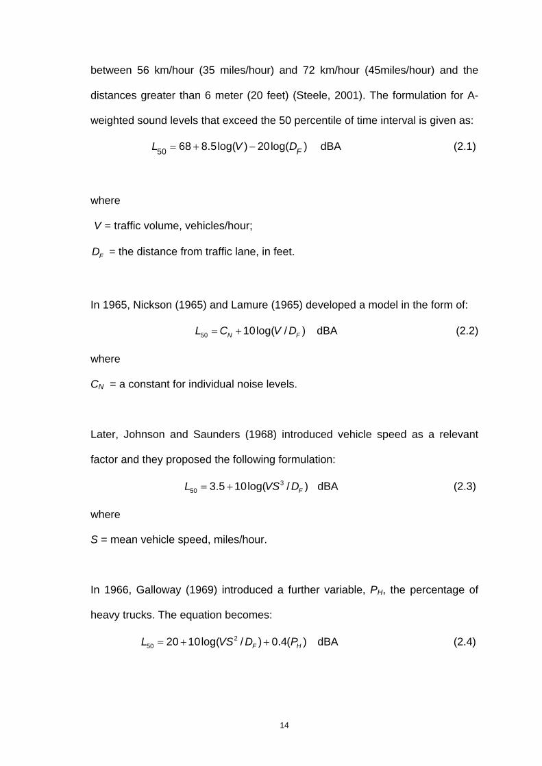
between 56 km/hour (35 miles/hour) and 72 km/hour (45miles/hour) and the

distances greater than 6 meter (20 feet) (Steele, 2001). The formulation for A-

weighted sound levels that exceed the 50 percentile of time interval is given as:

= + −50 68 8.5log( ) 20log( )FL V D dBA (2.1)

where

V = traffic volume, vehicles/hour;

FD = the distance from traffic lane, in feet.

In 1965, Nickson (1965) and Lamure (1965) developed a model in the form of:

= +50 10log( / )N FL C V D dBA (2.2)

where

CN = a constant for individual noise levels.

Later, Johnson and Saunders (1968) introduced vehicle speed as a relevant

factor and they proposed the following formulation:

= + 350 3.5 10log( / )FL VS D dBA (2.3)

where

S = mean vehicle speed, miles/hour.

In 1966, Galloway (1969) introduced a further variable, PH, the percentage of

heavy trucks. The equation becomes:

= + +250 20 10log( / ) 0.4( )F HL VS D P dBA (2.4)

15

Later developments introduced more variables and changes from L50 to L10 and

equivalent continuous level (Leq) over a chosen period (Steele, 2001).

Recent models predict the equivalent continuous sound level (Leq) under

interrupted and varying flow conditions. According to the reviews of Garcia

(2001) and Steele (2001), traffic noise prediction models in different countries

are designed to meet the requirements of government regulations. Those

prediction models are enhanced with more accurate physics and more realistic

computation in actual traffic flows. Detailed information for FHWA TNM (Menge

et al., 1998), which is used in this thesis, will be discussed in Section 2.3.1.

Section 2.3.2 is a review of others recent traffic noise models.

2.3.1 FHWA Traffic Noise Model

The Traffic Noise Model (TNM) is developed by the Federal Highway

Administration (FHWA) for predicting noise levels in the vicinity of highways and

to design highway noise barriers (Menge, 1998). This model is known as a

state-of-the-art computer program and developed by advance acoustics and

computer technology in modeling highway traffic noise (FHWA, 2002). In year

1998, the FHWA TNM, version 1.0 was released by FHWA to replace the

highway noise analysis program, Standard Method In Noise Analysis (STAMINA

2.0) (Anderson et al., 1998; Harris et al., 2000). The FHWA TNM is derived

from the STAMINA 2.0 program (Bowlby et al., 1982) and has several

substantial improvements. The improvements include provision for acceleration,

stop signs, toll booths, input of user-defined vehicles using their reference

energy mean emission level (REMEL) data, etc (Steele, 2001).

16

Five classes of vehicle are used in this FHWA model; they are

automobiles, medium trucks, heavy trucks, buses and motorcycles. To calculate

sound levels for entire traffic streams, FHWA TNM incorporates energy-

averaged vehicle noise emissions for each vehicle type (Menge et al., 1998).

Based on FHWA TNM technical manual (Menge et al., 1998), TNM needs three

constants to compute A-weighted noise-level emissions: A, B and C. It also

needs fourteen additional constants to convert these A-weighted noise-level

emissions to 1/3rd-otave-band spectra: D1, D2, E1, E2, F1, F2, G1, G2, H1, H2,

I1, I2, J1 and J2. Each vehicle type’s total measured noise emissions take into

account the whole frequency spectrum. The general REMEL equation is a

function of speed and frequency for each type of vehicles (i) as follows:

+Δ +Δ= +

− + + + + +

+ +

+ +

+ +

+ +

+ +

( ) /10 ( ) /10/10

2

3

4

5

6

( , ) 10log[10 (0.6214 )(10 )]( 1 2 ) 1 2 ( 1 2 )log( 1 2 )(log )( 1 2 )(log )( 1 2 )(log )( 1 2 )(log )( 1 2 )(log )

c bC E B EAE i i

i i i

i

i

i

i

i

L s f sK K s D D s E E s f

F F s f

G G s f

H H s f

I I s f

J J s f

dBA (2.5)

where

f = nominal 1/3rd-octave-band center frequency, in Hetz;

is = vehicle speed, in kilometer/hour;

A = the slope of tire/pavement noise portion of regression curve;

+ Δ bB E = the height of the tire/pavement noise portion of the regression curve;

+ Δ cC E = the height of the engine/exhaust noise portion of the regression

equation, which is independent of vehicle speed;

17

1D to 2J = constants of the sixth-order polynomial fit curve for the 1/3rd spectra;

K1 and K2 = the calibration of the resulting A-weighted levels from the sixth-

order polynomial fit.

Several adjustments are made to the emission level to account for traffic

flow, distance and shielding in FHWA TNM (Menge et al., 1998). The following

equation is the equivalent sound level over one hour time period, (1 h)AeqL

which involved those adjustments for different vehicle types:

= + + + ( )(1 h) Aeq i traff i d sL EL A A A dBA (2.6)

where

ELi = the vehicle noise emission;

Atraff(i) = the adjustment for traffic flow, the vehicle volume and speed;

Ad = the adjustment for distance between the roadway and receiver and for

the length of the roadway;

As = the adjustments for all shielding and ground effects between the roadway

and the receiver.

TNM has been updated several times and the latest version is TNM

Version 2.5 (Lau et al., 2004; Ning, 2005). TNM Version 2.5 has the improved

implementation to the vehicle emission level database. More comprehensive

methodologies are applied in correcting the measured emission back to the

source (Lau et al., 2004). The diffraction algorithm parameters are also

improved in the latest version. Table 2.1 shows the FHWA TNM release

versions since year 1998 until 2004.

18

Table 2.1: FHWA TNM versions

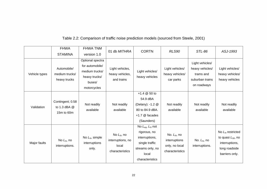
2.3.2 Other Traffic Noise Models

There are some other noise models such as CORTN, RLS-90, MITHRA,

StL-86 version 1 and ASJ Method 1993 that are used by different countries.

Calculation of Road Traffic Noise (CORTN) is developed for the prediction of

traffic noise in the United Kingdom Department of the Environment (Bies and

Hansen, 2003). This model assumes a line source and constant speed traffic.

The adjustments that apply in the model include percentage of heavy vehicle,

traffic speed, gradient, road surface and propagation. The acceleration is not

taken into account in CORTN (Steele, 2001). Richtlinien fur den Larmschutz an

StraBen (RLS-90) (Guidelines for Noise Propagation on Streets) is a noise

prediction model used in Germany (Steele, 2001). The attenuation in the noise

propagation is calculated with usual ray tracing methods in RLS-90 model.

MITHRA, developed by a French firm, contains an extensive ray-tracing

procedure. This commercial software package takes into account ground effects,

diffraction, reflection, topography, building and barrier (Steele, 2001). StL-86

version 1 is developed by the Swiss Federal Office of Environmental Protection.

The model includes corrections for the reflection from building, attenuations of

Year Model TNM version 1.0;

1998 TNM version 1.0a; TNM version 1.0b.

2000 TNM version 1.1 2002 TNM version 2.0 2003 TNM version 2.1 2004 TNM version 2.5

19

building and obstacles, usual distance effects and angle of road open to

receiver. The Acoustic Society of Japan has developed ASJ Method 1993 to

predict a pseudo – L50 from free-flowing road traffic. This software contains 2

types of methods; they are A-Method and B-Method. A-Method is a direct

method of calculating the equivalent sound level (Leq), and deriving the pseudo-

L50 from the results. B-Method is an empirical method which is only valid for

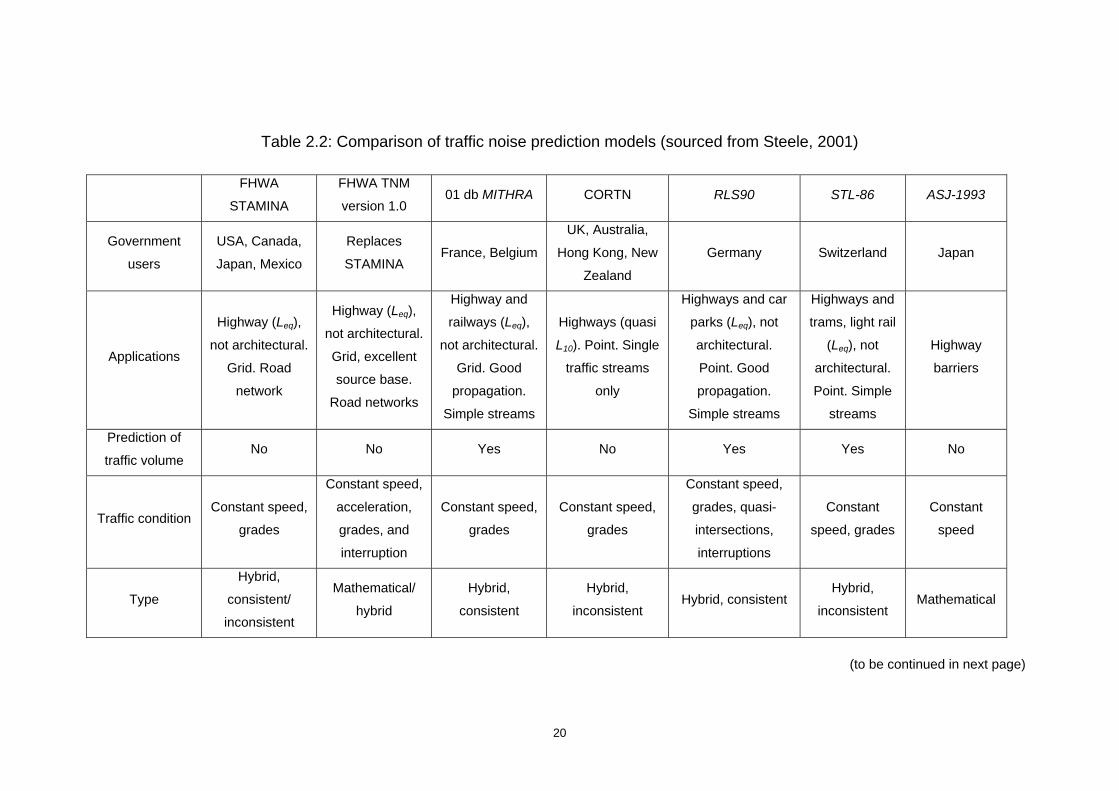
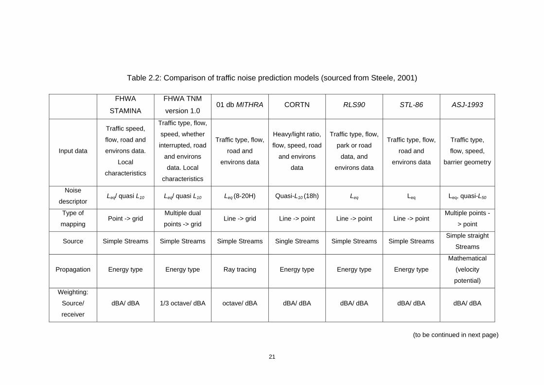
distances that are far from the line source. Table 2.2 provides the comparison of

FHWA STAMINA, FHWA TNM version 1.0, MITHRA, CORTN, RLS90, STL-86

and ASJ-1993 by Steele (2001).

20

Table 2.2: Comparison of traffic noise prediction models (sourced from Steele, 2001)

(to be continued in next page)

FHWA

STAMINA

FHWA TNM

version 1.0 01 db MITHRA CORTN RLS90 STL-86 ASJ-1993

Government

users

USA, Canada,

Japan, Mexico

Replaces

STAMINA France, Belgium

UK, Australia,

Hong Kong, New

Zealand

Germany Switzerland Japan

Applications

Highway (Leq),

not architectural.

Grid. Road

network

Highway (Leq),

not architectural.

Grid, excellent

source base.

Road networks

Highway and

railways (Leq),

not architectural.

Grid. Good

propagation.

Simple streams

Highways (quasi

L10). Point. Single

traffic streams

only

Highways and car

parks (Leq), not

architectural.

Point. Good

propagation.

Simple streams

Highways and

trams, light rail

(Leq), not

architectural.

Point. Simple

streams

Highway

barriers

Prediction of

traffic volume No No Yes No Yes Yes No

Traffic condition Constant speed,

grades

Constant speed,

acceleration,

grades, and

interruption

Constant speed,

grades

Constant speed,

grades

Constant speed,

grades, quasi-

intersections,

interruptions

Constant

speed, grades

Constant

speed

Type

Hybrid,

consistent/

inconsistent

Mathematical/

hybrid

Hybrid,

consistent

Hybrid,

inconsistent Hybrid, consistent

Hybrid,

inconsistent Mathematical

21


(to be continued in next page)

FHWA

STAMINA

FHWA TNM


Input data

Traffic speed,

flow, road and

environs data.

Local

characteristics

Traffic type, flow,

speed, whether

interrupted, road

and environs

data. Local

characteristics

Traffic type, flow,

road and

environs data

Heavy/light ratio,

flow, speed, road

and environs

data

Traffic type, flow,

park or road

data, and

environs data

Traffic type, flow,

road and

environs data

Traffic type,

flow, speed,

barrier geometry

Noise

descriptor Leq/ quasi L10 Leq/ quasi L10 Leq (8-20H) Quasi-L10 (18h) Leq Leq Leq, quasi-L50

Type of

mapping Point -> grid

Multiple dual

points -> grid Line -> grid Line -> point Line -> point Line -> point

Multiple points -

> point

Source Simple Streams Simple Streams Simple Streams Single Streams Simple Streams Simple Streams Simple straight

Streams

Propagation Energy type Energy type Ray tracing Energy type Energy type Energy type

Mathematical

(velocity

potential)

Weighting:

Source/

receiver

dBA/ dBA 1/3 octave/ dBA octave/ dBA dBA/ dBA dBA/ dBA dBA/ dBA dBA/ dBA

22


FHWA

STAMINA

FHWA TNM


Vehicle types

Automobile/

medium trucks/

heavy trucks

Optional spectra

for automobile/

medium trucks/

heavy trucks/

buses/

motorcycles

Light vehicles,

heavy vehicles,

and trains

Light vehicles/

heavy vehicles

Light vehicles/

heavy vehicles/

car parks

Light vehicles/

heavy vehicles/

trams and

suburban trains

on roadways

Light vehicles/

heavy vehicles/

heavy vehicles

Validation

Contingent; 0.58

to 1.3 dBA @

15m to 60m

Not readily

available

Not readily

available

+1.4 @ 50 to

54.9 dBA

(Delany): -1.2 @

80 to 84.9 dBA.

+1.7 @ facades

(Saunders)

Not readily

available

Not readily

available

Not readily

available

Major faults No LN, no

interruptions.

No LN, simple

interruptions

only.

No LN, no

interruptions, no

local

characteristics

No Leq, LN not

rigorous, no

interruptions,

single traffic

streams only, no

local

characteristics

No. LN, no

interruptions

only, no local

characteristics

No. LN, no

interruptions.

No LN restricted

to quasi L50, no

interruptions,

long roadside

barriers only.

23

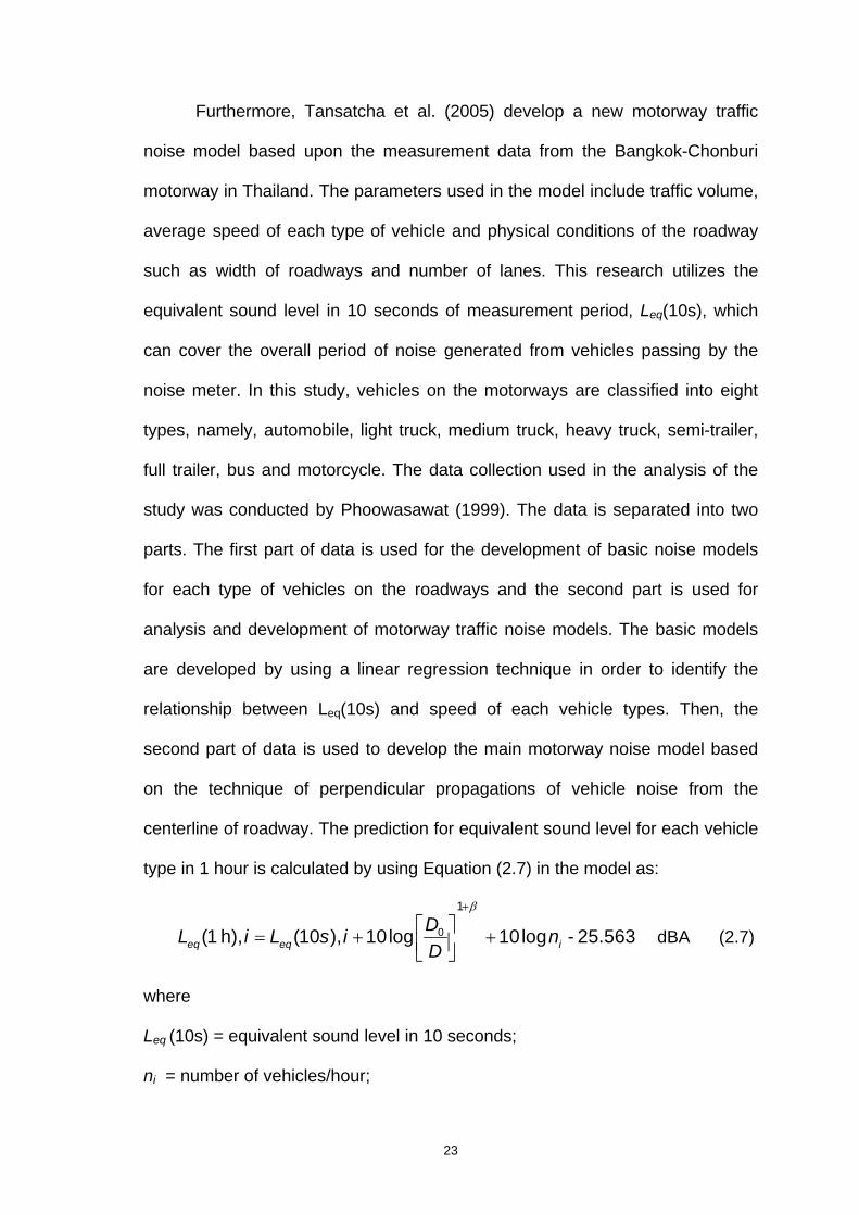
Furthermore, Tansatcha et al. (2005) develop a new motorway traffic

noise model based upon the measurement data from the Bangkok-Chonburi

motorway in Thailand. The parameters used in the model include traffic volume,

average speed of each type of vehicle and physical conditions of the roadway

such as width of roadways and number of lanes. This research utilizes the

equivalent sound level in 10 seconds of measurement period, Leq(10s), which

can cover the overall period of noise generated from vehicles passing by the

noise meter. In this study, vehicles on the motorways are classified into eight

types, namely, automobile, light truck, medium truck, heavy truck, semi-trailer,

full trailer, bus and motorcycle. The data collection used in the analysis of the

study was conducted by Phoowasawat (1999). The data is separated into two

parts. The first part of data is used for the development of basic noise models

for each type of vehicles on the roadways and the second part is used for

analysis and development of motorway traffic noise models. The basic models

are developed by using a linear regression technique in order to identify the

relationship between Leq(10s) and speed of each vehicle types. Then, the

second part of data is used to develop the main motorway noise model based

on the technique of perpendicular propagations of vehicle noise from the

centerline of roadway. The prediction for equivalent sound level for each vehicle

type in 1 hour is calculated by using Equation (2.7) in the model as:

β+

⎡ ⎤= + +⎢ ⎥⎣ ⎦0

1

(1 h), (10 ), 10log 10log - 25.563eq eq iDL i L s i nD

dBA (2.7)

where

Leq (10s) = equivalent sound level in 10 seconds;

ni = number of vehicles/hour;

24

D = perpendicular distance from observer to the centre line of the traffic lane;

D0 = the reference distance (15meters);

β = ground effect adjustment.

The new model has two advantages. The first advantage is that the

speed of the vehicles can be excluded from the main model. Secondly, this

model provides a simple format with fewer parameters. Tansatcha et al. (2005)

conclude that the motorway traffic noise model performs well in a statistical

goodness-of-fit test against the field data and therefore, it can be used

effectively in traffic noise prediction projects in Thailand.

2.4 Noise Control Barriers

Noise mitigation by barriers is a popular mitigation measure for

environmental protection in both urban and rural areas. Currently, much

research has been conducted to develop efficient noise control barriers and to

assess its performance in mitigating noise pollutions. The choice of noise

control methods depends on the cost, effectiveness and feasibility (Ming, 2005).

To maximize the acoustic performance of a noise barrier, the mathematical

prediction scheme is needed to calculate sound reduction by barriers (Li and

Wong, 2005). Usually, the total reduction provided by the barrier is calculated

by insertion loss (IL). IL is the difference between two sound pressure levels

measured at the same point in space before and after a muffler has been

installed (Bell and Bell, 1994).

noise modeling in universiti sains malaysia and offshore

Documents