noise and contrast discrimination in computed …kmh-lanl.hansonhub.com/publications/rsb81.pdfnoise...
TRANSCRIPT
CHAPTER 113
Noise and computed Kenneth M. Hanson
contrast discrimination in tomography
Image noise Random noise
Statistical noise Electronic noise Roundoff errors
Artifactual noise Structural noise
Properties of CT noise Noise power spectrum
Fourier analysis-MTF and noise power spectrum Visual example Dependence on reconstruction algorithm and NEQ Results for a commercial scanner
Autocorrelation function Noise granularity
Definition Relationship to noise power spectrum Results for a commercial scanner
rms noise CT noise and dose
Dose dependence Dose efficiency
Dose specification DNEQ Results for a commercial scanner
Detectability in the presence of CT noise Detection task Optimum receiver
Detection sensitivity index, d' Application to CT Example
Human observer Three-dimensional aspects
Conclusion
The x-ray computed tomographic (CT) scanner has made it possible to detect the presence of lesions of very low contrast (New et al., 1973). This dramatic improvement in detection capability over most conventional forms of x-ray imaging is a result of the following innovations: (1) the noise in the reconstructed C T images is significantly reduced through the use of efficient x-ray detectors and
electronic processing, thereby improving the utilization of the radiation dose. (2) T h e images can be displayed with enhanced contrast, thus overcoming the minimum contrast threshold of the human eye. (3) The C T reconstruction technique almost completely eliminates the superposition of anatomic structures, leading to a reduction of "struc- tural" noise.
I t is the random noise in a C T image that ultimately limits the ability of the radiologist to discriminate between two regions of different density. Because of its unpre- dictable nature, such noise cannot be completely eliminated from the image and will always lead to some uncertainty in the interpretation of the image. There is strong evidence that much of the random noise in present-day C T scanners is due to the statistical inaccuracies arising from the detec- tion of a finite number of transmitted x-ray quanta. The properties of this statistical noise in C T images will be dis- cussed in this chapter. The goal will be to characterize the noise content in a way that is closely related to the detection capabilities inherent in the image.
I t will be shown in the discussion of' the optimum re- ceiver that the ability to detect a large-area object in a C T image is chiefly dependent on the NEQ, the total number of noise-equivalent quanta detected per unit length in the projections used to reconstruct that image. As such, it is not the fineness with which the x rays are detected in the projections (related to spatial resolution) but simply the effective total number of detected x rays that influences the large-area contrast sensitivity of the C T reconstruction. For a fixed, large-area contrast sensitivity, then, an increase in spatial resolution does not imply the necessity for higher dose! NEQ, which characterizes the low-frequency proper- ties of noise in a C T image, can be determined from a C T noise image by measuring either the noise-power spectrum or the noise granularity function.
Since, for a given C T geometry, the number of trans- mitted x-ray quanta is proportional to the dose, the magni- tude of the statistical noise depends on the dose. A figure- of-merit for dose utilization will be developed that can be used to compare the dose efficiencies of various C T scan- ners.
in Radiology of the Skull and Brain, Vol. 5: Technical Aspects of Computed Tomography, T. H. Newton and D. G. Potts, eds. (C. V. Mosby, St. Louis, 1981) ISBN 0-8016-3662-0 (v. 5)
3942 General theory of computed tomography
Fig. 113-1. Block diagram of the steps involved in obtaining a CT image.
Fig. 113-2. Three scans of a contrast sensitivity phantom taken on a GE CTIT 7800 scanner at various milliampere-second values: A, 77. B, 307. C , 1152. The low contrast in the largest sector, 0.25%, is achieved by the partial volume effect. For this scanner higher dose leads to lower noise and improved contrast sensitivity. (Courtesy F. A. DiBianca, General Electric Co.)
X-ray source
Reconstructior? - - X-ray detector
Display - Camera -- -dpl and film
Signal processing
-
Noise and contrast discrimination in computed tomography 3943
IMAGE NOISE
There are several types of image "noise" that can inter- fere with the interpretation of an image. In the discussion of the types and sources of noise present in C T images it is helpful to consider the various steps in the production of a C T image as presented in Fig. 113-1. Although noise may infiltrate and corrupt the data at any point in the C T process, the ultimate source of noise is the random, statisti- cal noise, arising from the detection of a finite number of x-ray quanta in the projection measurements.
Random noise
Image mottling, o r fluctuations in the image density that change from one image to the next in an unpredictable and random manner, may be termed random noise. The radiologist is familiar with random noise in the form of radiographic mottle found in standard radiographs taken with fast screen-film combinations (Ter-Pogossian, 1967, p. 249).
Statistical noise
The energy in x-radiation is transmitted in the form of individual chunks of energy called quanta. Hence the response of an x-ray detector is actually the result of de- tecting a finite number of x-ray quanta. The number of detected quanta will vary from one measurement to the next, not because of inadequacies in the detection appara- tus, but because of statistical fluctuations that naturally arise in the "counting" process. As more quanta are de- tected in each measurement, the relative accuracy of each measurement improves. Statistical noise in x-ray images arises from the fluctuations inherent in the detection of a finite number of x-ray quanta. Statistical noise may also be called quantum noise and is often referred to as quan- tum mottle in film radiography.
Statistical noise clearly represents a fundamental limita- tion in x-ray radiographic processes. T h e only way to re- duce the effects of statistical noise is to increase the number of detected x-ray quanta. Normally this is achieved by in- creasing the number of transmitted x rays through an in- crease in dose. Fig. 113-2 shows a series of scans taken on a GE CT /T 7800 scanner* using a phantom designed to test contrast sensitivity. The reduction in the noise caused by increasing the x-ray exposure (milliampere-seconds) is graphically demonstrated.
Electronic noise
In processing electric signals, electronic circuits inevitably add some noise to the signals. Analog circuits, those which process continuously varying signals, are most susceptible to additional noise. Thus the stage most likely to inject additional electronic noise in Fig. 113-1 is that of analog signal processing. The difficulty of noise suppression is compounded by the fact that for some types of x-ray detec- tors, the electronic signals are very small. There is evidence (Cohen, 1979) that many commercially available C T scan- ners are sufficiently well engineered to reduce the con- -
*General Electric Medical Systems Division, Milwaukee, Wis.
tribution of electronic noise under normal operating condi- tions to a fraction of the statistical noise contribution. The signals are converted to digital or discrete form in the signal-processing step and then sent to a computer for reconstruction.
Digital circuits, those which process discrete signals as in digital computers, are relatively impervious to electronic noise problems.
Roundoff errors
Although digital computers are not subject to electronic noise, they d o introduce noise in the reconstruction process through roundoff errors. T h e errors arise from the lim- ited number of bits used to represent numbers in the com- puter. For example, the product of two numbers must be rounded off to the least significant bit used in the com- puter's representation of the number. Roundoff errors can normally be kept at a n insignificant level either through choice of a computer with enough bits per word o r through proper programming. It should be pointed out that in some C T scanners the final reconstruction is stored with the least significant bit equal to one C T number (0.1 % of the linear attenuation coefficient of water). This should not influence the accuracy significantly so long as the rms noise is greater than one C T number.
Roundoff errors can and d o occur in the display stage (Fig. 113-I), since C T display units can display only a fixed number of discrete brightness levels. As an example, a unit that has only 32 brightness levels will result in an increment size of about 0.05 optical density units (OD) on exposed radiography film. A difference of 0.05 OD produces a luminance contrast of 12%. Since under optimum condi- tions the human observer can discern objects at contrasts of less than 0.004 OD (Chapter 115; Burgess et al., 1979), such a unit can limit the observer's ability to interpret the film, particularly for wide display windows (100 or more C T units). This limitation may be circumvented by the use of a narrow window.
Artifactual noise
T h e wide variety of artifacts that can be produced by C T scanners is presented in Chapter 114. Artifacts might be viewed as a form of noise in that they interfere with the interpretation of the C T image. Their presence is often indicated by a readily identifiable pattern, for example, in the case of streak artifacts. These identifiable artifacts d o not produce random noise, since they should be unchanged in repeated scans of the same object. However, there are instances in which regions of a reconstruction may experi- ence an increase in variance due to nonapparent artifacts (Sheridan et al., 1980). Artifactual noise will not be con- sidered further here.
Structural "noise"
Density variations in the object being imaged that inter- fere with the diagnosis are sometimes referred to as struc- tural "noise" or structural clutter. In standard radiography a large amount of structural clutter is produced by the superposition of various anatomic structures, for example,
3944 General theory of computed tomography
the image of rib bones overlaps that of the lung in a stan- dard chest radiograph. The C T technique eliminates most of this superposition, but the radiologist should be aware that partial contributions may be introduced by structures that principally appear in adjacent C T slices.
Some organs, such as the liver, may have density varia- tions within them that have the appearance of' random noise. Although the texture pattern of the organ may not be reproducible from one C T scan to the next because of patient motion, this type of structural variation is, of course, not random. Indeed, the classification of' this den- sity variation as a type of noise is ill-advised, since the varia- tion is intrinsic to the object itself. The study of the tissue texture may be interesting for its potential diagnostic value (Pullan et al., 1978).
PROPERTIES OF CT NOISE
The consequences of statistical noise in C T reconstruc- tions have been discussed by numerous authors (Shepp and Logan, 1974; Cho et al., 1975; Huesman, 1975; Tanaka and Iinuma, 1975, 1976; Barrett et al., 1976; Brooks and DiChiro, 1976; Chesler et al., 1977; Hanson, 1977; Hues- man, 1977; Joseph, 1977, 1978; Hanson and Boyd, 1978; Riederer et al., 1978; Hanson, 1979a; Wagner et al., 1979). Several of these authors have pointed out that the process of reconstruction leads to some peculiar characteristics of the noise in C T images. The properties of statistical (quan- tum) noise in C T reconstructions will be explored in this discussion. Although the precise random noise pattern of any image cannot be predicted a priori, it is possible to characterize the average behavior of the noise by a variety of methods. Some of these methods give a complete de- scription of the noise characteristics, such as the noise power spectrum or the noise autocorrelation function, whereas others give only a partial description, such as rms noise. It will develop that the noise fluctuation in one pixel of a C T reconstruction is not independent of the noise fluctuations in other pixels. Rather, the fluctuations in two separate pixels are, on the average, correlated.
Noise power spectrum
The noise power spectrum is a frequency representation of the correlations present in the noise. The ramplike na- ture of the noise power spectrum expected for C T recon- structions will be derived for the filtered back projection algorithm. It will be shown that noise power spectra of EM1 CT5005 reconstructions possess this ramplike be- havior at low frequencies.
Fourier analysis - MTF and noise power spectrum
Any signal may be thought of as a sum of sine waves of appropriate frequency, amplitude, and position (phase). This decomposition of a signal into its frequency compo- nents is called Fourier analysis (see Chapter 110). It is often helpful to apply Fourier analysis to imaging systems (cam- eras, television, x-ray radiographs, etc.) because of the ease with which the imaging properties of various stages of the systems combine in their frequency representations. T o be sure, Fourier analysis is only useful for linear systems, but
most imaging techniques are approximately linear for small changes in signal amplitudes. A good introduction to the application of Fourier analysis to radiography may be found in Johns and Cunningham (1969).
The modulation transfer function (MTF) is the frequen- cy decomposition of a system's line spread response func- tion.* The latter is the output of the imaging system when an extremely narrow line is used as input; for example, the radiograph produced of a very fine metal wire. Since in the frequency representation of an infinitely narrow line all frequencies are present with equal contribution, the MTF actually measures the frequency response of the sys- tem. Most MTFs are fairly close to unity at low frequen- cies, meaning that these frequencies are transferred through the imaging system with almost no degradation. T h e MTFs of all physical systems will eventually fall to zero at high frequencies. This means that the high frequencies are not preserved by the imaging system and simply are not present in the final image. Since perfectly sharp edges re- quire infinitely high frequencies to represent them, the loss of the high frequencies results in blurred edges. Thus the MTF is the frequency representation of the sharpness of the system.
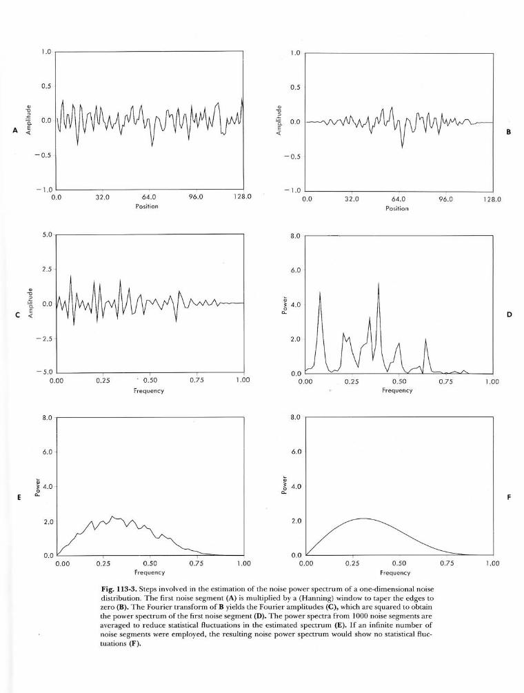
The noise power spectrum is related to the frequency decomposition of the image noise. The method of obtain- ing the noise power spectrum will be outlined to clarify the relationship. First, an image containing nothing but the noise to be analyzed is decomposed into its two-dimensional frequency components. These components, called the Fourier amplitudes, are then squared to obtain the "power" contribution at each frequency. This result is averaged with the results obtained from other similar images to arrive finally at the average noise power for each frequency, or, in other words, the noise power spectrum. The noise power spectrum is therefore proportional to the average (or mean) square value of the frequency amplitudes of the noise. Fig. 1 13-3 illustrates the computational procedure for obtaining the noise power spectrum of a one-dimen- sional noise sample. Note that the square of the amplitude is used instead of the amplitude itself, since the average value of the amplitude is zero while the average value of the squared amplitude is not. The noise power spectrum is often referred to as the Wiener spectrum. Often the re- sponse of the system is assumed to be circularly symmetric. Then the two-dimensional noise power spectrum may be reduced to a one-dimensional spectrum that is a function of only the radial frequency (distance from zero frequency in two-dimensions).
The noise found in conventional radiographs is typified by a noise power spectrum that is roughly constant over a wide range of frequencies. Such a noise power spectrum is called "white" in analogy to white light, which contains a mixture of light of all frequencies within the visible spec-
*The two-dimensional MTF is the frequency decomposition of a system's point spread function. The latter is the output of the imaging system when an extremely small point is used as input. A one-dimensional section of the two-dimensional MTF is obtained from the line spread function.
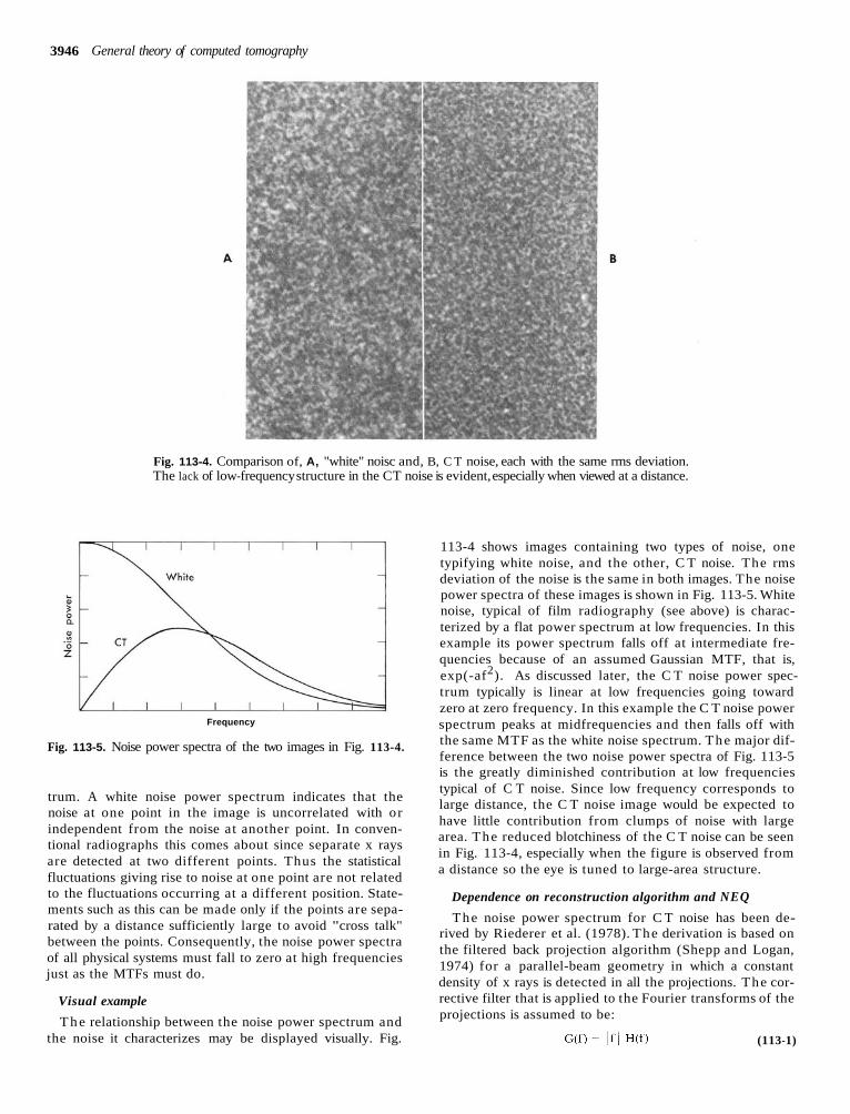
3946 General theory of computed tomography
Fig. 113-4. Comparison of, A, "white" noisc and, B, C T noise, each with the same rms deviation. The lack of low-frequency structure in the CT noise is evident, especially when viewed at a distance.
Frequency
Fig. 113-5. Noise power spectra of the two images in Fig. 113-4.
trum. A white noise power spectrum indicates that the noise at one point in the image is uncorrelated with or independent from the noise at another point. In conven- tional radiographs this comes about since separate x rays are detected at two different points. Thus the statistical fluctuations giving rise to noise at one point are not related to the fluctuations occurring at a different position. State- ments such as this can be made only if the points are sepa- rated by a distance sufficiently large to avoid "cross talk" between the points. Consequently, the noise power spectra of all physical systems must fall to zero at high frequencies just as the MTFs must do.
Visual example
T h e relationship between the noise power spectrum and the noise it characterizes may be displayed visually. Fig.
113-4 shows images containing two types of noise, one typifying white noise, and the other, C T noise. The rms deviation of the noise is the same in both images. The noise power spectra of these images is shown in Fig. 113-5. White noise, typical of film radiography (see above) is charac- terized by a flat power spectrum at low frequencies. In this example its power spectrum falls off at intermediate fre- quencies because of an assumed Gaussian MTF, that is, exp(-af2). As discussed later, the C T noise power spec- trum typically is linear at low frequencies going toward zero at zero frequency. In this example the C T noise power spectrum peaks at midfrequencies and then falls off with the same MTF as the white noise spectrum. The major dif- ference between the two noise power spectra of Fig. 113-5 is the greatly diminished contribution at low frequencies typical of C T noise. Since low frequency corresponds to large distance, the C T noise image would be expected to have little contribution from clumps of noise with large area. The reduced blotchiness of the C T noise can be seen in Fig. 113-4, especially when the figure is observed from a distance so the eye is tuned to large-area structure.
Dependence on reconstruction algorithm and NEQ
The noise power spectrum for C T noise has been de- rived by Riederer et al. (1978). The derivation is based on the filtered back projection algorithm (Shepp and Logan, 1974) for a parallel-beam geometry in which a constant density of x rays is detected in all the projections. The cor- rective filter that is applied to the Fourier transforms of the projections is assumed to be:
G(f) = I f 1 H(f) (113-1)
Noise and contrast discrimination in computed tomography 3947
where f is the frequency and H is a weighting (or apodiza- tion) factor. The principal restriction on H is that it be nearly unity for very low frequencies f. It may be shown that the noise power spectrum S for statistical C T noise can be written as follows (Riederer et al., 1978; Hanson, 1979a; Wagner et al., 1979):
where NEQ, the number of noise-equivalent quanta, is the total effective number of x-ray quanta detected per unit distance along the projections (summed over all the projec- tion measurements). If there is no source of noise other than statistical and the reconstruction algorithm is efficient, then NEQ will be just the total number-of detected x rays per unit projection length. The presence of other sources of noise can reduce NEQ compared with the actual number of detected quanta. Also, the measurement of the x-ray flu- ence by means of an energy-integrating detector (as is done on essentially all commercial CT scanners) leads to a slight reduction (-10%) in NEQ compared to that attainable through x-ray counting. In equation 113-2 it is assumed that the reconstructed image is the linear attenuation co- efficient lr, given in units of (cm-1). Then S will be dimen- sionless and NEQ will have dimension (cm-1), as it should.
Equation 113-2 indicates that the noise power spectra of CT reconstructions should have a ramplike dependence at low frequencies (where H = 1). The slope of S at low fre- quencies is determined by NEQ. As such, NEQ may be used to characterize the large-area, low-contrast detection capabilities of C T images (see discussion of optimum re- ceiver). It shall be shown that equation 113-2 implies there is no loss in detection performance in a filtered back projec- tion reconstruction compared to the input projection data for large objects. As more quanta are detected, S will be reduced inversely and the C T image noise will diminish.
The dependence of S on the weighting factor H of the algorithm should be noted. |/ H Imay be regarded as the MTF associated with the reconstruction algorithm in the absence of binning problems associated with the finite size of the reconstruction pixels (Hanson, 1979b). The MTF of the complete scanner system is the product of all the MTFs that contribute to the spatial resolution of the final image. For many CT scanner systems the dominant contribution is the MTF associated with the finite width of the radiation beam used in the projection measurements (Barnes et al., 1979). Thus, although the total noise of the C T scanner is closely related to the spatial resolution of the reconstruc- tion algorithm, it may have only a weak dependence on the overall spatial resolution. It should also be realized that the image noise is not dependent on the pixel size except insofar as the latter affects the choice of H.
Results for a commercial scanner
The noise power spectrum has been calculated for an EM1 CT5005 scanner* to demonstrate that it has the form
*EM1 Medical, Inc., 4000 Commercial Dr., Northbrook, Ill. 60062.
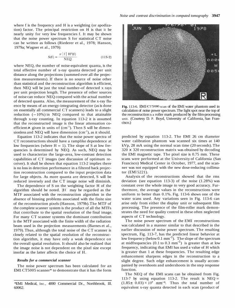
Fig. 113-6. EM I CT50 scan of the EMI water phantom used in calculation of noise power spectrum. The light spot near the top of the reconstruction is a roller mark produced by the film-processing unit. (Courtesy D. P. Boyd, University of California, San Fran- cisco.)
predicted by equation 113-2. The EMI 26 cm diameter water calibration phantom was scanned six times at 140 kVp, 28 mA using the normal scan time (20 seconds). The 320 x 320 reconstruction matrix was obtained by decoding the EMI magnetic tape. The pixel size is 0.75 mm. These scans were performed at the University of California (San Francisco) Medical Center in October, 1977, and the scan- ner was not equipped with the new dose-reducing collima- tor (EMI 5221).
Analysis of the reconstructions showed that the rms deviation (see equation 113-3) of the noise (1.28%) was constant over the whole image to very good accuracy. Fur- thermore, the average values in the reconstructions were uniform to better than 0.1%. Fig. 113-6 shows one of the water scans used. Any variations seen in Fig. 113-6 can arise only from either the display unit or subsequent film processing. The presence of the film-roller mark demon- strates the need for quality control in these often neglected aspects of C T technology.
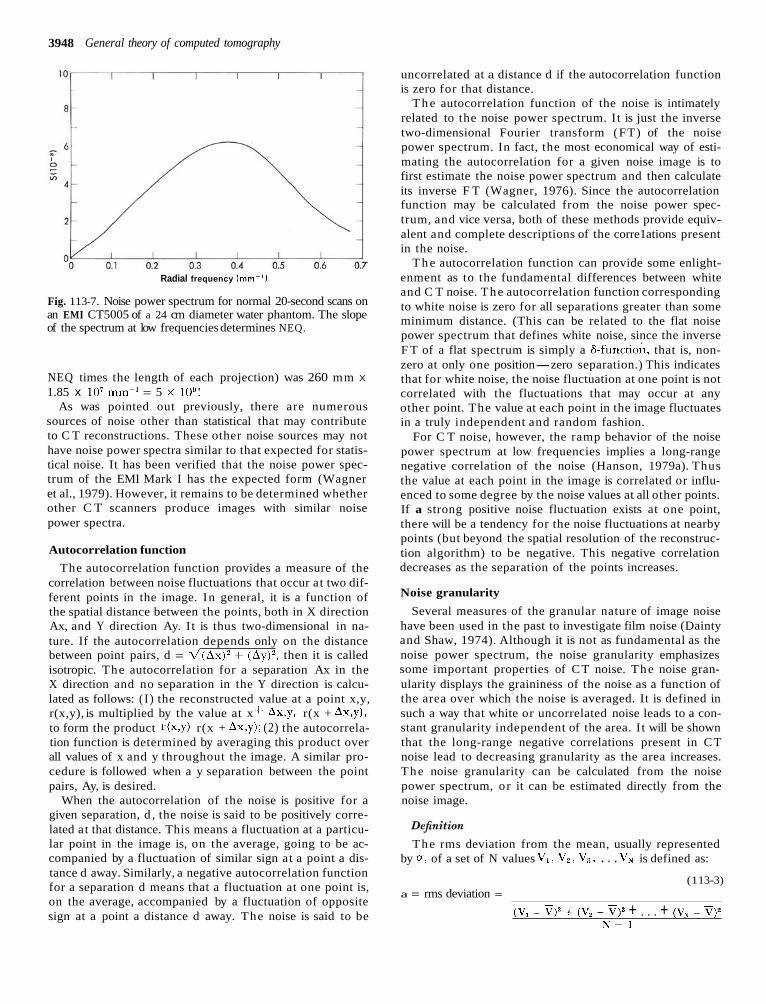
The noise power spectrum of the EMI reconstructions was calculated in a manner similar to that described in the earlier discussion of noise power spectrum. The resulting spectrum, Fig. 113-7, has the predicted linear behavior at low frequency (below 0.1 mm-1). The slope of the spectrum at midfrequencies (0.1 to 0.3 mm-1) is greater than at low frequency, indicating that EMI has used a value of H which is greater than 1 at these frequencies. The resulting edge enhancement sharpens edges in the reconstruction to a slight degree. Such edge enhancement is usually accom- panied by overshoots and undershoots in the step response function.
The NEQ of the EM1 scans can be obtained from Fig. 113-7 by using equation 113-2. The result is NEQ = (1.85 ? 0.03) x lo7 mm-l. Thus the total number of equivalent x-ray quanta detected in each scan (product of
3948 General theory of computed tomography
Radial frequency (mm-'1
Fig. 113-7. Noise power spectrum for normal 20-second scans on an EMI CT5005 of a 24 cm diameter water phantom. The slope of the spectrum at low frequencies determines NEQ.
NEQ times the length of each projection) was 260 mm X
1.85 x lo7 mm-' = 5 x lo9! As was pointed out previously, there are numerous
sources of noise other than statistical that may contribute to C T reconstructions. These other noise sources may not have noise power spectra similar to that expected for statis- tical noise. It has been verified that the noise power spec- trum of the EMI Mark I has the expected form (Wagner et al., 1979). However, it remains to be determined whether other C T scanners produce images with similar noise power spectra.
Autocorrelation function
The autocorrelation function provides a measure of the correlation between noise fluctuations that occur at two dif- ferent points in the image. In general, it is a function of the spatial distance between the points, both in X direction Ax, and Y direction Ay. I t is thus two-dimensional in na- ture. If the autocorrelation depends only on the distance between point pairs, d = AX)' + ( A Y ) ~ , then it is called isotropic. The autocorrelation for a separation Ax in the X direction and no separation in the Y direction is calcu- lated as follows: ( I ) the reconstructed value at a point x,y, r(x,y), is multiplied by the value at x + Ax,y, r(x + Ax,y), to form the product r(x,y) r(x + Ax,y) (2) the autocorrela- tion function is determined by averaging this product over all values of x and y throughout the image. A similar pro- cedure is followed when a y separation between the point pairs, Ay, is desired.
When the autocorrelation of the noise is positive for a given separation, d , the noise is said to be positively corre- lated at that distance. This means a fluctuation at a particu- lar point in the image is, on the average, going to be ac- companied by a fluctuation of similar sign at a point a dis- tance d away. Similarly, a negative autocorrelation function for a separation d means that a fluctuation at one point is, on the average, accompanied by a fluctuation of opposite sign at a point a distance d away. The noise is said to be
uncorrelated at a distance d if the autocorrelation function is zero for that distance.
T h e autocorrelation function of the noise is intimately related to the noise power spectrum. I t is just the inverse two-dimensional Fourier transform (FT) of the noise power spectrum. In fact, the most economical way of esti- mating the autocorrelation for a given noise image is to first estimate the noise power spectrum and then calculate its inverse F T (Wagner, 1976). Since the autocorrelation function may be calculated from the noise power spec- trum, and vice versa, both of these methods provide equiv- alent and complete descriptions of the corre1ations present in the noise.
T h e autocorrelation function can provide some enlight- enment as to the fundamental differences between white and C T noise. The autocorrelation function corresponding to white noise is zero for all separations greater than some minimum distance. (This can be related to the flat noise power spectrum that defines white noise, since the inverse F T of a flat spectrum is simply a 6-function, that is, non- zero at only one position-zero separation.) This indicates that for white noise, the noise fluctuation at one point is not correlated with the fluctuations that may occur at any other point. The value at each point in the image fluctuates in a truly independent and random fashion.
For C T noise, however, the ramp behavior of the noise power spectrum at low frequencies implies a long-range negative correlation of the noise (Hanson, 1979a). Thus the value at each point in the image is correlated or influ- enced to some degree by the noise values at all other points. If a strong positive noise fluctuation exists at one point, there will be a tendency for the noise fluctuations at nearby points (but beyond the spatial resolution of the reconstruc- tion algorithm) to be negative. This negative correlation decreases as the separation of the points increases.
Noise granularity
Several measures of the granular nature of image noise have been used in the past to investigate film noise (Dainty and Shaw, 1974). Although it is not as fundamental as the noise power spectrum, the noise granularity emphasizes some important properties of CT noise. The noise gran- ularity displays the graininess of the noise as a function of the area over which the noise is averaged. It is defined in such a way that white or uncorrelated noise leads to a con- stant granularity independent of the area. I t will be shown that the long-range negative correlations present in CT noise lead to decreasing granularity as the area increases. The noise granularity can be calculated from the noise power spectrum, or it can be estimated directly from the noise image.
The rms deviation from the mean, usually represented by u, of a set of N values V , , V,, V,, . . . VN is defined as:
(1 13-3) a = rms deviation =
(V, - q2 + (V2 - V)2 + . . . + (VN - V)2 N - 1
Noise and contrast discrimination in computed tomography 3949
where the average or mean value V is:
The rms deviation u is a measure of the amount of scatter or variation in the values away from their mean V. Suppose the mean value of the reconstruction is calculated for an area A at N locations throughout the image. Then the noise granularity shall be defined here as:
G(A) = crA 6 (1 13-5)
where U A is the rms deviation (equation 113-3) of these means and A is the area. Thus the noise granularity is a measure of the amount of scatter in the area-averaged values. G, defined by equation 113-5, is Selwyn's granu- larity coefficient (Selwyn, 1935) divided by $.
It is convenient to extend the definition of noise granu- larity to include weighted means. The weighted mean is calculated by multiplying the reconstruction values by a weight function and then summing (or integrating) the re- sulting products. In equation 113-5, u.., is then the rms deviation of the weighted means. The weight function is a function of x and y, which usually is nonzero only within a certain distance from the central pixel. It is conveniently normalized such that the sum of the weights is unity, and it is characterized by an effective area A. For the strict un- weighted mean the weight function is a constant over the area A and zero elsewhere. The weighted mean then yields the average value over the area A. A more interesting weight function is, for example, pyramidal in shape. The largest weight is given to the central pixel, and the weight function drops linearly to zero in all directions away from the center. The application of this weight function will be demonstrated later.
Relationship to noise power spectrum
G may be readily calculated in terms of the noise power spectrum S, since -4 is simply the integral over frequency of S multiplied by an appropriate function (the square of the frequency representation of the weighting function used in calculating the mean). Thus S should be considered as a more fundamental measure of the noise characteristics than G. However, there may be some practical advantages, such as ease of calculation, to the use of G. Moreover, G is useful because it demonstrates the effect on the rms noise (uA) of averaging over different areas.
The relationship between G and S may be used to show that G for large areas is principally determined by the mag- nitude of S at low frequencies. For CT noise the ramplike dependence of S at low frequency, or equivalently the long- range negative correlation in the noise, implies that (Han- son, 1979a):
where NEQ is the number of equivalent x-ray quanta de- tected per unit length in the projections (equation 113-2). It should be noted that equation 113-6 is a good approxi- mation for weighting functions that have tapered edges,
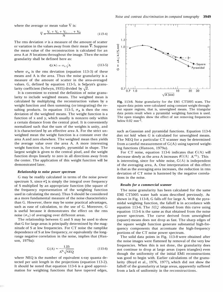
Fig. 113-8. Noise granularity for the EM1 CT5005 scans. The square data points were calculated using constant weight through- out square regions, that is, unweighted means. The triangular data points result when a pyramidal weighting function is used. The open triangles show the effect of not removing frequencies below 0.02 mm-1.
such as Gaussian and pyramidal functions. Equation 113-6 does not hold when G is calculated for unweighted means. The NEQ for a particular CT scanner may be determined from a careful measurement of G (A) using tapered weight- ing functions (Hanson, 1979a).
For CT noise, equation 113-6 indicates that G(A) will decrease slowly as the area A increases (G(A) A-%). This is interesting, since for white noise, G(A) is independent of the averaging area, A. One interpretation of this effect is that as the averaging area increases, the reduction in rms deviation of CT noise is hastened by the negative correla- tions in the noise.
Results for a commercial scanner
The noise granularity has been calculated for the same EMI CT5005 water bath scans described previously. As shown in Fig. 113-8, G falls off for large A. With the pyra- midal weighting function, the falloff is in accordance with equation 113-6. The NEQ obtained from this curve using equation 113-6 is the same as that obtained from the noise power spectrum. The curve derived from unweighted (square) means does not drop as fast. The sharp edges of the square weight function generate substantial high-fre- quency components that accentuate the high-frequency portions of the CT noise power spectrum.
The solid data points in Fig. 113-8 were obtained after the noise images were flattened by removal of the very low frequencies. When this is not done, the granularity does not continue to drop at large areas (open triangles) even though the uniformity of the initial EM1 reconstructions was good to begin with. Earlier calculations of the granu- larity (Boyd et al., 1976, 1977), which did not show the falloff of the granularity at large areas, apparently suffered from a lack of uniformity in the reconstructions.
3950 General theoy of computed tomography
rms noise
Frequently the rms deviation (equation 113-3) of the noise is quoted for C T reconstructions. It should be clear that the rms noise is not a complete characterization of C T noise, since it ignores the frequency dependence of the noise. Specifically, the rms noise depends critically on the weighting factor H( f ) used in the reconstruction algorithm, which will vary from one C T scanner to the next. It will be shown that the ability to detect large-area objects is related to the low-frequency noise power content, which is rela- tively unaffected by H(f) . Thus detectability is not simply related to the rms noise.
The rms noise may be calculated from the noise power spectrum (by Parseval's theorem) as the square root of the total noise power:
Since a2 is the integral of the noise power spectrum, it con- tains no information about the frequency dependence of the noise.
CT NOISE AND DOSE
The statistical noise in C T reconstructions is closely re- lated to the dose. T h e dose efficiency of a given scanner may be obtained by comparison of its delivered dose to that required by an ideal x-ray scanner to achieve the same NEQ. This dose efficiency summarizes all contributions to the utilization of the delivered dose such as x-ray beam col- limation, compensation wedges, detector efficiency, and signal processing, as well as the degrading effects of poly- chromaticity, detection of scattered radiation, electronic noise, and inefficient reconstruction algorithms.
Dose dependence
The dependence of the statistical noise power spectrum on dose is indicated in equation 113-2. Since the number of detected quanta (NEQ) is proportional to the number of initial quanta, and hence the dose, D, it is concluded that S is inversely proportional to dose. Then, by equation 113- 7, the rms value of the statistical noise should be inversely proportional to ,/6. This is not always the case for com- mercial C T scanners.
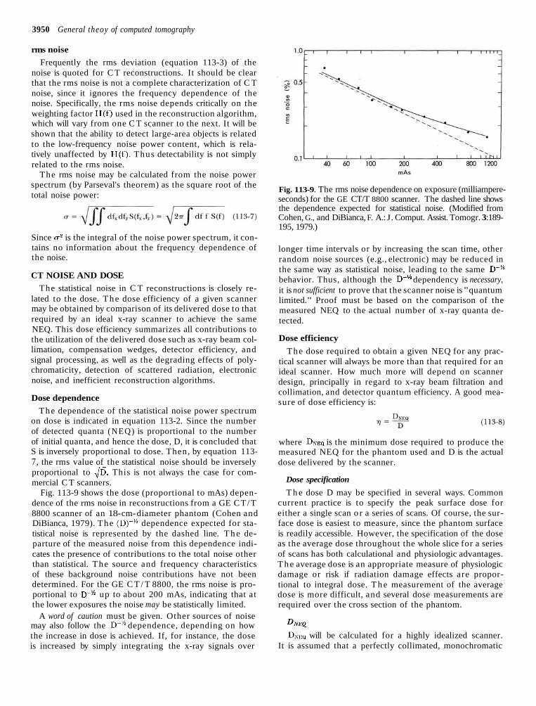
Fig. 113-9 shows the dose (proportional to mAs) depen- dence of the rms noise in reconstructions from a GE CT /T 8800 scanner of an 18-cm-diameter phantom (Cohen and DiBianca, 1979). The (D)-" dependence expected for sta- tistical noise is represented by the dashed line. T h e de- parture of the measured noise from this dependence indi- cates the presence of contributions to the total noise other than statistical. The source and frequency characteristics of these background noise contributions have not been determined. For the GE C T / T 8800, the rms noise is pro- portional to D-% up to about 200 mAs, indicating that at the lower exposures the noise may be statistically limited.
A word of caution must be given. Other sources of noise
may also follow the D-% dependence, depending on how the increase in dose is achieved. If, for instance, the dose is increased by simply integrating the x-ray signals over
Fig. 113-9. The rms noise dependence on exposure (milliampere- seconds) for the GE CT/T 8800 scanner. The dashed line shows the dependence expected for statistical noise. (Modified from Cohen, G., and DiBianca, F. A.: J. Comput. Assist. Tomogr. 3:189- 195, 1979.)
longer time intervals or by increasing the scan time, other random noise sources (e.g., electronic) may be reduced in the same way as statistical noise, leading to the same D-% behavior. Thus, although the D-" dependency is necessary, it is not sufficient to prove that the scanner noise is "quantum limited." Proof must be based on the comparison of the measured NEQ to the actual number of x-ray quanta de- tected.
Dose efficiency
The dose required to obtain a given NEQ for any prac- tical scanner will always be more than that required for an ideal scanner. How much more will depend on scanner design, principally in regard to x-ray beam filtration and collimation, and detector quantum efficiency. A good mea- sure of dose efficiency is:
where DNEQ is the minimum dose required to produce the measured NEQ for the phantom used and D is the actual dose delivered by the scanner.
Dose specification
T h e dose D may be specified in several ways. Common current practice is to specify the peak surface dose for either a single scan o r a series of scans. Of course, the sur- face dose is easiest to measure, since the phantom surface is readily accessible. However, the specification of the dose as the average dose throughout the whole slice for a series of scans has both calculational and physiologic advantages. T h e average dose is an appropriate measure of physiologic damage or risk if radiation damage effects are propor- tional to integral dose. T h e measurement of the average dose is more difficult, and several dose measurements are required over the cross section of the phantom.
D N E ~ DNEQ will be calculated for a highly idealized scanner.
It is assumed that a perfectly collimated, monochromatic
Noise and contrast discrimination i n computed tomography
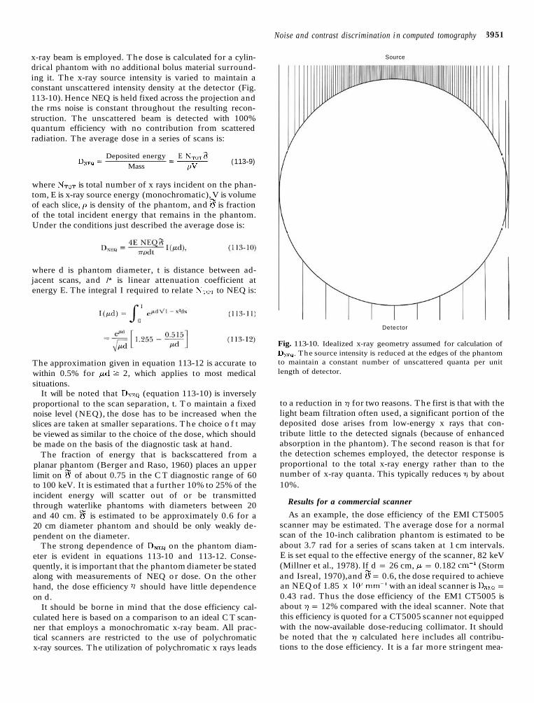
x-ray beam is employed. The dose is calculated for a cylin- drical phantom with no additional bolus material surround- ing it. The x-ray source intensity is varied to maintain a constant unscattered intensity density at the detector (Fig. 113-10). Hence NEQ is held fixed across the projection and the rms noise is constant throughout the resulting recon- struction. The unscattered beam is detected with 100% quantum efficiency with no contribution from scattered radiation. The average dose in a series of scans is:
Deposited energy E N~~~ 3 DNEQ = -- -
Mass ( 1 13-9)
PV
where NToT is total number of x rays incident on the phan- tom, E is x-ray source energy (monochromatic), V is volume of each slice, p is density of the phantom, and 8 is fraction of the total incident energy that remains in the phantom. Under the conditions just described the average dose is:
where d is phantom diameter, t is distance between ad- jacent scans, and /* is linear attenuation coefficient at energy E. The integral I required to relate NTOT to NEQ is:
The approximation given in equation 113-12 is accurate to within 0.5% for p d 2 2, which applies to most medical situations.
It will be noted that DNEP (equation 1 13-10) is inversely proportional to the scan separation, t. T o maintain a fixed noise level (NEQ), the dose has to be increased when the slices are taken at smaller separations. T h e choice o f t may be viewed as similar to the choice of the dose, which should be made on the basis of the diagnostic task at hand.
The fraction of energy that is backscattered from a planar phantom (Berger and Raso, 1960) places an upper limit on 8 of about 0.75 in the C T diagnostic range of 60 to 100 keV. It is estimated that a further 10% to 25% of the incident energy will scatter out of or be transmitted through waterlike phantoms with diameters between 20 and 40 cm. 8 is estimated to be approximately 0.6 for a 20 cm diameter phantom and should be only weakly de- pendent on the diameter.
The strong dependence of DNEQ on the phantom diam- eter is evident in equations 113-10 and 113-12. Conse- quently, it is important that the phantom diameter be stated along with measurements of NEQ o r dose. O n the other hand, the dose efficiency 7 should have little dependence on d.
It should be borne in mind that the dose efficiency cal- culated here is based on a comparison to an ideal C T scan- ner that employs a monochromatic x-ray beam. All prac- tical scanners are restricted to the use of polychromatic x-ray sources. The utilization of polychromatic x rays leads
Source
Detector
Fig. 113-10. Idealized x-ray geometry assumed for calculation of DNEQ The source intensity is reduced at the edges of the phantom to maintain a constant number of unscattered quanta per unit length of detector.
to a reduction in -/I for two reasons. The first is that with the light beam filtration often used, a significant portion of the deposited dose arises from low-energy x rays that con- tribute little to the detected signals (because of enhanced absorption in the phantom). The second reason is that for the detection schemes employed, the detector response is proportional to the total x-ray energy rather than to the number of x-ray quanta. This typically reduces 7 by about 10%.
Results for a commercial scanner
As an example, the dose efficiency of the EMI CT5005 scanner may be estimated. The average dose for a normal scan of the 10-inch calibration phantom is estimated to be about 3.7 rad for a series of scans taken at 1 cm intervals. E is set equal to the effective energy of the scanner, 82 keV (Millner et al., 1978). If d = 26 cm, /* = 0.182 cm-' (Storm and Isreal, 1970), and 8 = 0.6, the dose required to achieve an NEQ of 1.85 X lo7 mm-' with an ideal scanner is DNEQ =
0.43 rad. Thus the dose efficiency of the EM1 CT5005 is about 7 = 12% compared with the ideal scanner. Note that this efficiency is quoted for a CT5005 scanner not equipped with the now-available dose-reducing collimator. It should be noted that the 7) calculated here includes all contribu- tions to the dose efficiency. It is a far more stringent mea-
3952 General theory of computed tomography
sure of dose efficiency than just the "detector efficien- cy."
DETECTABILITY IN THE PRESENCE OF CT NOISE
It is clear from Fig. 113-2 that a reduction in the mag- nitude of the noise leads to improved detection of contrast differences. But suppose the same phantom were scanned on another scanner with completely different spatial resolu- tion and, more important, a completely different recon- struction algorithm. What measure of noise would allow comparison of the ability to discriminate contrast differ- ences in the two scans? This is the central issue in the de- scription of noise. It is important to use parameters to char- acterize the noise that are directly and simply related to de- tectability. In this discussion the close relationship between N E Q and the detection of large-area objects is described. This relationship is established for the optimum receiver, which fully takes into account the characteristics of CT noise. The connection between the detection performance of the optimum receiver and that of the human observer is not well documented. However, it is expected that the two performances will track each other in a relative evalu- ation of similar images. Thus the basis of comparison dic- tated by the optimum receiver will probably be useful in the comparison of clinical images.
Detection task
To simplify matters, only the binary decision problem will be considered here. The decision to be made is whether a specific object is present at a specific location. Further- more, it is assumed that the background on which the ob- ject is superimposed is completely specified. This detection problem is exemplified by the phantom in Fig. 113-2 in which circular objects are present on a flat background. However, the presence of a row of circles rather than a single circle alters the problem slightly and complicates the analysis of the results. The binary decision case may be ex- tended to the multiple decision problem (Goodenough, 1975; Goodenough and Metz, 1974) or to the problem of the search for objects within an image (Wagner, 1977). Although the binary decision problem represents a gross simplification of the clinical detection situation, at present this simplification is necessary to permit theoretical analysis and psychophysical testing.
Clinical diagnosis clearly relies heavily on the ability of the radiologist to recognize patterns. The general pattern recognition problem is very difficult to model in full detail. However, the ability to detect component parts of a pattern must form the basis of pattern recognition. Thus it is hoped and expected that results obtained from analysis of the simple detection problems often encountered in psycho- physical testing will be relevant to the more complex clin- ical situation.
Optimum receiver Detection sensitivity index, d ' Given an object to be detected in the presence of a spe-
cific type of noise, the best detection performance that is possible may be determined through application of signal
detection theory (Whalen, 1971; Van Trees, 1968; Wagner, 1978). The best decision criterion that can be used in a given detection problem is referred to as the "optimum' receiver" in signal detection theory. The optimum receiver will depend on the situation at hand. In particular, the op- timum receiver must take into account the properties of the noise to be "optimum." It is often possible to charac- terize the detection performance of the optimum receiver without actually constructing or implementing the detec- tion criterion.
The detection performance of any detector applied to a given detection task may be summarized by its receiver operating characteristic (ROC) curve. The ROC curve is a plot of the probability of a "true positive" response versus the probability of a "false positive" response (Chapter 115; Green and Swets, 1966). For additive, Gaussian distributed noise, the ROC curve for the binary decision problem may be completely specified by a single parameter, the detec- tion sensitivity index d'. The d ' depends on the object's contrast, size, and shape as well as on the magnitude and correlations of the noise. For the optimum receiver d ' may be expressed in terms of the frequency representation of the object R(f) as follows (Barnard, 1972):
where S is the noise power spectrum (see earlier discussion of dependence on reconstruction algorithm and NEQ) . It is observed that dfOPTIMUM is determined by the frequency sum or integral of the ratio of the signal power to the noise power. It should be noted that the design of an optimum receiver depends critically on the properties of the noise. Thus a receiver that is optimum for white (uncorrelated) noise will not be optimum for CT noise.
The plausibility of equation 113-13 may be illustrated for two limiting cases. For the first case the following situ- ation will be considered: S is zero for some finite frequency interval in which the object power I R / is not zero. The integrand in equation 113-13 would then be infinite over that frequency interval yielding an infinite value for d'opTIMuw This is reasonable, since the optimum receiver would only have to check the image power (after the known background was removed) in the appropriate frequency interval. If there was any power present, it could only be due to the object. The optimum receiver could never make a mistake! Hence, dlOPTIMUM = m. In the second case, the situation in which I R 1 is zero over some finite frequency interval is considered. Equation 113-13 indicates that noise power in that frequency interval will not influence the op- timum receiver. Again, this is reasonable, since the opti- mum receiver can remove these frequency intervals from consideration by Fourier transformation of the image fol- lowed by zeroing out the Fourier amplitudes in the relevant frequency interval.
Equation 1 13- 13 leads one to an interesting conclusion concerning the trade-off between noise magnitude and spa- tial resolution. It is well known that the rms noise may be reduced by smoothing the image. Smoothing also results in a loss of spatial resolution, which is supposed to make it more difficult to detect small objects or to locate the posi-
Noise and contrast discrimination i n computed tomography 3953
tions of sharp edges. However, image smoothing is equiva- lent to the multiplication of the frequency representation of the image by a filter, which generally reduces the high- frequency components of the image. Since both / RI "nd S arc affected by the filter in the same way, equation 113-13 indicates that d'opT,MuM is not altered by the smoothing pro- cess, unless the filter is zero for some finite range of fre- quencies where I R I "s not zero. Thus the performance of the optimum receiver is not affected by smoothing (unless information is lost by a zero filter). Indeed, it is not neces- sary to trade off between low noise and high spatial resolu- tion for the optimum receiver.
These statements concerning the optimum receiver may or may not have bearing on what might be expected of a human observer. For example, the human observer may suffer critical band masking between frequency intervals (see Chapter 115). Thus it is unlikely that the human ob- server could make use of information in one frequency interval that through filtering was reduced by a factor 100 relative to neighboring frequency intervals. Of course, the "optimum receiver," being a conceptual entity, would have no difficulty recouping the information in the attenuated frequency band.
Although the optimum receiver may not realistically characterize the performance of the human observer, it provides the ultimate standard against which the human observer may be compared. If it is found that the perfor- mance of the human observer falls short of this ideal in the simple detection task envisioned, then it may prove useful to explore the reasons for the shortcomings of the human observer.
Application to CT
The application of signal detection theory to computed tomography leads to an interesting result (Hanson, 1979a). Of course, the projection data themselves may be used to detect the presence of an object within the projection field. It is found that when the totality of projection data is ana- lyzed by the optimum receiver, the resulting dlOPTIMUM is equal to or greater than the dfoPTIMuM obtained from anal- ysis of the reconstruction. In other words, the detection in a C T reconstruction of a specific object on a known back- ground can be no better than when the detection of the same object is based on the direct projection measurements. Furthermore, the detection performance based on an ef- ficient reconstruction can equal that based on the pro- jections. It has been shown that the filtered back projection algorithm is efficient, in this sense, for the detection of large objects (Hanson, 1979a, 1980). I n the practical case of reconstruction in a discrete pixel array from discretely sampled projections, there can be a loss of information leading to some degradation in detection sensitivity (Han- son, 1979b).
The frequency representation, R(f), of an object with large area is concentrated at low frequencies. Then equa- tion 113-13 indicates that the detection sensitivity of large- area objects will be principally determined by the low-fre- quency content of the' noise power. Since statistical C T noise has a ramplike noise power spectrum at low fre- quencies, the single parameter that characterizes the slope
of the ramp, NEQ, is a sufficient measure of the detection sensitivity for large objects. I t is found (Hanson, 1979a) that the optimum sensitivity index is:
7
d f O p T ~ ~ U ~ = A p A',/NEQ (113-14)
where A p is the average contrast of the object with an ef- fective area A. Equation 113-14 is a good approximation for most objects of large area (square, circle, etc.). The A'/" dependence of dlOPTlMUM should be noted. It arises from the ramplike nature of the C T noise power spectrum. For white noise (s = constant), d ' is proportional to A%.
Example
An example can illustrate the use of equation 113-14. Consider a 5 mm diameter cylinder placed in a water phan- tom with a 26 cm diameter. What is the value of d ' achieved by an EM1 CT5005 scanner if the reconstructed density of the cylinder differs from water by 0.4%? Since p = 0.019 mm-' for water, and the area of the reconstructed circle is A = n x 2.5' = 19.6 mm2, equation 113-14 gives:
For the binary decision problem, a d ' of 3.0 results in an ROC curve such that a true positive response can be made 93% of the time for a false positive probability of 7%. If the position of the cylinder is unknown, then its detection is made much more difficult by the necessity of a search pro- cedure. The resulting ROC curve would be much poorer than that for the binary decision case (Goodenough and Metz, 1974).
Human observer
The relationship between the detection capabilities of the ideal detector and those of the human observer has not been fully explored for images containing CT noise. It is possible that human observers may have shortcomings, particularly in their ability to integrate the noise over the object area. The unusual correlations present in C T recon- structions may prove difficult for the eye-brain to take into account. Several psychophysical studies (Hanson, 1977; Joseph, 1977, 1978; Chew et al., 1978; Orphanoudakis*) have shown that under certain circumstances observer de- tectability of large objects is improved by smoothing C T images. T h e reason for this improvement remains to be explained. Furthermore, the A-% dependence in the threshold contrast for a constant d ' predicted in equation 113-14 has not been verified for human observers (Cohen, 1979). The effects of altered viewing conditions and train- ing have yet to be investigated. Further discussion of this topic may be found in Chapter 1 15.
Three-dimensional aspects
T h e discussion of preceding sections dealt with the de- tection of a two-dimensional object in a single C T scan. In reality, however, the radiologic detection problem is three- dimensional in nature. The difficulties in detecting three-
*Personal communication, 1979.

3954 General theory of computed tomography
dimensional objects in C T scans a r e often referred t o as "partial volume" effects (Chapter 109). T o illustrate the problem, consider the detection of a sphere of diameter d immersed i n a uniform background of slightly lower density. I f t h e sphere happened to lie completely within a single C T slice, its effective reconstruction density would be less than its actual density because of the partial volume effect. But if adjacent slices happened to split the sphere in half, its reconstructed density would be halved relative to the case just described. In t h e latter situation, t h e detection of the sphere is made more difficult by t h e large reduction in its reconstruction density, particularly if each slice is viewed independently. A n improvement in detection could be attained by simply averaging t h e two slices, since the
rms noise would be reduced by a factor of -. This prob- k lem illustrates the desirability of a display system that allows full use o f t h e three-dimensional information available in C T (Hanson, 1979a).
CONCLUSION T h e detection limitations inherent in statistically limited
computed tomographic (CT) images have been described through the application of signal detection theory. T h e detectability of large-area, low-contrast objects has been shown to be chiefly dependent o n the low-frequency con- tent of the noise power spectral density. For projection data containing uncorrelated noise, the resulting ramplike, low- frequency behavior of the noise power spectrum of the C T reconstruction may be conveniently characterized by t h e density o f noise-equivalent quanta (NEQ) detected in t h e projection measurements. T h e NEQ for a given image can be determined either f rom a measurement of the noise power spectrum o r f rom the noise granularity computed with a n appropriate weighting function. T h e performance for the detection of large objects is as good in a n efficient reconstruction (e.g., filtered back projection) as that based o n the projection data. A measure of the efficiency of scanner dose utilization was presented that compares the average dose required by a n ideal x-ray scanner to obtain the measured NEQ to that delivered by the actual scanner.
REFERENCES Barnard, T . W.: Image evaluation by means of target recognition,
Phot. Sci. Eng. 16: 144-150, 1972. Barnes, G. T., Yester, M. V., and King, M. A,: Optimizing com-
puted tomography (CT) scanner geometry, Proc. SPIE Appl. Opt. Instr. in Medicine VII 173:225-237, 1979.
Barrett, H. H., Gordon, S. K., and Hershel, R. S.: Statistical limita- tions in transaxial tomography, Comput. Biol. Med. 6:307-323, 1976.
Berger, M. J., and Raso, D. J.: Monte Carlo calculations of gamma- ray backscattering, Radiat. Res. 12:20-37, 1960.
Boyd, D. P., Korobkin, M. T., and Moss, A.: Engineering status of computerized-tomographic scanning, Proc. SPIE Appl. Opt. Instr. in Medicine V 96:303-312, 1976.
Boyd, D. P., Margulis, A. R., and Korobkin, M. T.: Comparison of translate-rotate and pure rotary computed tomography (CT) body scanners, Proc. SPIE Appl. Opt. Instr. in Medicine VI 127:280-285, 1977.
Brooks, R. A,, and Di Chiro, G.: Statistical limitations in x-ray re- constructive tomography, Med. Phys. 3:237-340, 1976.
Burgess, A. E., Humphrey, K., and Wagner, R. F.: Detection of bars and discs in quantum noise, Proc. SPIE Appl. Opt. Instr. in Medicine VII 173:34-40, 1979.
Chesler, D. A,, Riederer, S. J., and Pelc, N. J.: Noise due to photon counting statistics in computed x-ray tomography, J. Comput. Assist. Tomogr. 1:64-74, 1977.
Chew, E., Weiss, G. H., Brooks, R. A . , and Di Chiro, G.: Effect of CT noise on detectability of test objects, Am. J. Roentgenol. 131:681-685, 1978.
Cho, Z. H., Chan, J. K., Hall, E. L., Kruger, R. P., and McCaughey, D. G.: A comparative study of 3-D image reconstruction algo- rithms with reference to number of projections and noise fil- tering, IEEE Trans. Nucl. Sci. NS-22:344-358, 1975.
Cohen, G.: : Contrast-detail-dose analysis of six different computed tomographic scanners, J. Comput. Assist. Tomogr. 3:197-203, 1979.
Cohen. G., and DiBianca. F. A.: The use of contrast-detail-dose evaluation of image quality in a computed tomographic scanner, J. Comput. Assist. Tomogr. 3:189-195, 1979.
Dainty, J. C., and Shaw, R.: Image science; principles, analysis and evaluation of photographic-type imaging processes, Lon- don, 1974, Academic Press, Inc. Ltd.
Goodenough, D. J.: Objective measures related to ROC curves, Proc. SPIE Appl. Opt. Instr. in Medicine III 47:134-141, 1975.
Goodenough, D. J., and Metz, C. E.: Effect of listening interval on auditory detection performance, J. Acoust. Soc. Am. 55:lll- 116, 1974.
Green, D. M., and Swets, J. A,: Signal detection theory and psycho- physics, New York, 1966, John Wiley & Sons, Inc.
Hanson, K. M.: Detectability in the presence of computed tomo- graphic reconstruction noise, Proc. SPIE Appl. Opt. Instr. in Medicine VI 127:304-312, 1977.
Hanson, K. M.: Detectability in computed tomographic images, Med. Phys. 6:441-451, 1979a.
Hanson, K. M.: The detective quantum efficiency of C T recon- struction: the detection of small objects, Proc. SPIE Appl. Opt. Instr. in Medicine VII 173:291-298, 1979b.
Hanson, K. M.: On the optimality of the filtered backprojection algorithm, J. Comput. Assist. Tomogr. 4:361-363, 1980.
Hanson, K. M., and Boyd, D. P.: The characteristics of computed tomographic reconstruction noise and their effect on detectabil- ity, IEEE Trans. Nucl. Sci. NS-25:160-173, 1978.
Huesman, R. H.: Analysis of statistical errors for transverse section reconstruction, Lawrence Berkeley Laboratory report #4278, 1975, University of California, Berkeley, Calif.
Huesman, R. H.: The effects of a finite number of projection angles and finite lateral sampling of projections on the propa- gation of statistical errors in transverse section reconstruction, Phys. Med. Biol. 22:511-521, 1977.
Johns, H. E., and Cunningham, J. R.: The physics of radiology, ed. 3, Springfield, 1969, Charles C Thomas.
Joseph, P. M.: Image noise and smoothing in computed tomog- raphy (CT) scanners, Proc. SPIE Appl. Opt. Instr. in Medicine VI 127:43-49, 1977, and in Opt. Eng. 17:396-399, 1978.
Millner, M. R., Payne, W. H., Waggener, R. G., McDavid, W. D., . Dennis, M. J., and Sank, V. J.: Dctcrmination of effective ener- gies in CT calibration, Med. Phys. 5:543-545, 1978.
New, P. F. J., Scott, W. R., Schnur, J. A., Davis, K. R., and Taveras, J. M.: Computerized axial tomography with the EM1 scanner, Radiology 110:109-123, 1973.
Pullan, B. R., Fawcitt, R. A., and Isherwood, I.: Tissue charac- terization by an analysis of the distribution of attenuation values
Noise and contrast discrimination i n computed tomography 3955
in computed tomography scans: a preliminary report, J. Comput. Assist. Tomogr. 2:49-54, 1978.
Riederer, S. J., Pelc, N. J., and Chesler, D. A.: The noise power spectrum in computed x-ray tomography, Phys. Med. Biol. 23: 446-454, 1978.
Selwyn, E. W. H.: A theory of graininess, Photographic J. 75:571, 1935.
Shepp, L. A., and Logan, B. F.: The Fourier reconstruction of a head section, IEEE Trans. Nucl. Sci. NS-21:21-43, 1974.
Sheridan, W., Keller, M., O'Conner, C., Brooks, R. A . , and Han- son, K. M.: Evaluation of edge-induced artifacts in C T scanners, Med. Phys. 7: 108- 11 1, 1980.
Storm, E., and Isreal, H. I.: Photon cross sections from 1 keV to 100 MeV for elements Z = 1 to Z = 100, U.S. Atomic Energy Commission, Nucl. Data Tables A7:565-681, 1970.
Tanaka, E., and Iinuma, T. A.,: Corrective functions for optimiz- ing the reconstructed image in transverse section scan, Phys. Med. Biol. 20:789-798, 1975.
Tanaka, E., and Iinuma, T. A.: Corrective functions and statistical
noises in transverse section picture reconstruction, Comput. Biol. Med. 6:295-306, 1976.
Ter-Pogossian, M. M.: The physical aspects of diagnostic radiol- ogy, New York, 1967, Harper & Row, Publishers.
Van Trees, H. L.: Detection, estimation and modulation theory, New York, 1968, John Wiley & Sons, Inc.
Wagner, R. F.: Fast Fourier digital quantum mottle analysis with application to rare earth intensifying screen systems, Med. Phys. 4:157-162, 1976.
Wagner, R. F.: Toward a unified view of radiological imaging sys- tems. 11. Noisy images, Med. Phys. 4:279-296, 1977.
Wagner, R. F.: Decision theory and the detail signal-to-noise ratio of Otto Schade, Photogr. Sci. Eng. 22:41-46, 1978.
Wagner, R. F., Brown, D. G., and Pastel, M. S.: The application of information theory to the assessment of computed tomography, Med. Phys. 6:83-94, 1979.
Whalen, A. D.: Detection of signals in noise, New York, 1971, Academic Press, Inc.
Volume Five
Radiology of the skull and brain TECHNICAL ASPECTS OF COMPUTED TOMOGRAPHY
EDITED BY
Thomas H. Newton, M.D. Professor of Radiology, Neurology and Neurosurgery; Chief, Section of Neuroradiology, University of California School of Medicine, San Francisco, California
D. Gordon Potts, M.D. Professor of Radiology, Cornell University Medical College; Attending Radiologist, The New York Hospital, New York, New York
with 863 illustrations
The C. V. Mosby Company ST. LOUIS T O R O N T O LONDON 1981