noaa-16 satellite fragmentation in orbit: genesis of the

Advances in Aerospace Science and Applications. ISSN 2277-3223 Volume 7, Number 1 (2017), pp. 37-47 © Research India Publications http://www.ripublication.com

NOAA-16 Satellite Fragmentation in Orbit: Genesis

of the Gabbard Diagram and Estimation of the

Intensity of Breakup

Arjun Tan*, Robert C. Reynolds1 and Marius Schamschula

Department of Physics, Alabama A & M University, Normal, AL 35762, U.S.A. 1VP for Advanced Programs, STAR Dynamics Inc., Hilliard, OH 43026, U.S.A.

Abstract

This study analyzes the fragmentation of the NOAA-16 meteorological satellite which occurred in November 2015. The Gabbard diagram of the fragments cataloged through the end of that year reveals a pristine ‘X’ form expected for fragmentations of satellites in a near-circular orbit. The formation of the two sides of the X is deduced, including the slopes of the arms of the X, the forbidden zone, the smear of points above and below the X, and the equation of the hyperbolic envelopes of the points obtained. The magnitudes of the limiting velocity perturbations in the down-range and radial directions are estimated from that diagram. It is concluded that the NOAA-16 breakup exemplifies a new category of satellite fragmentation, different from the explosive fragmentation of the upper stage rocket bodies in orbit.

1. INTRODUCTION

On 25 November 2015 at 09:50 GMT, the decommissioned U.S. weather satellite NOAA-16 (International Designator 2000-055A; USSTRATCOM Catalog Number 26536) suffered a substantial breakup in orbit [1]. The fragmentation was similar to those suffered by the DMSP F-13 satellite earlier in that year and the DMSP F-11 satellite in 2004, and was attributed to the explosion of an over-charged Nickel-Cadmium battery [2]. These fragmentations constitute a third category of in-orbit satellite fragmentations, the first two being (1) The explosion of rocket bodies due to ignition of residual fuel, customarily called ‘Low-Intensity Fragmentations;’ and (2) The intentional fragmentation of satellites using explosives, referred to as ‘High-Intensity Fragmentations.’ The Gabbard diagram of the first 136 cataloged NOAA-16

mailto:[email protected]

38 Arjun Tan, Robert C. Reynolds and Marius Schamschula

fragments exhibited a classic ‘X’ shape expected for fragments from a circular orbit [1, 2]. The hyperbolic shape of the outer-most fragments is also evident. This paper describes the formation of the X-shaped Gabbard diagram bounded by hyperbolic envelopes that has been observed in satellite fragmentations many times before and frequently mentioned in the literature but never explained mathematically.

2. GABBARD DIAGRAM OF NOAA-16 FRAGMENTS

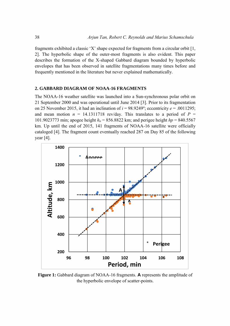
The NOAA-16 weather satellite was launched into a Sun-synchronous polar orbit on 21 September 2000 and was operational until June 2014 [3]. Prior to its fragmentation on 25 November 2015, it had an inclination of i = 98.9249o; eccentricity e = .0011295; and mean motion n = 14.1311718 rev/day. This translates to a period of P = 101.9023773 min; apogee height ha = 856.8822 km; and perigee height hp = 840.5567 km. Up until the end of 2015, 141 fragments of NOAA-16 satellite were officially cataloged [4]. The fragment count eventually reached 287 on Day 85 of the following year [4].

Figure 1: Gabbard diagram of NOAA-16 fragments. A represents the amplitude of

the hyperbolic envelope of scatter-points.

200

400

600

800

1000

1200

1400

96 98 100 102 104 106 108

Alt

itu

de

, km

Period, min

Apogee

Perigee

A

A

NOAA-16 Satellite Fragmentation in Orbit: Genesis of the Gabbard Diagram… 39

Fig. 1 shows the Gabbard diagram of the first 138 fragments. The data points were calculated from the earliest orbital elements of the fragments following the fragmentation available at spacetrack.org [4]. Not shown in the figure are three fragments having periods under 95 min which were severely affected by atmospheric drag. Within the figure are two fragments with periods 98.56 min (satellite numbers 41098 and 41099) similarly affected and rendered nearly circular.

The Gabbard diagram is a widely used tool in the study of satellite fragmentation. Yet, its formation has seldom, if ever, been discussed in the literature. The Gabbard diagram was invented by John Gabbard to study the fragmentation of Delta upper stages in orbit [5]. It is a plot of the apogee and perigee heights of the fragments against their periods. For fragmentation from a circular orbit, it has the shape of an ‘inclined X’ formed by a horizontal straight line and a straight line having a positive slope, the two lines intersecting at the coordinates of the fragmenting satellite (P0, h0). The right hand side of the X, to the right of (P0, h0), is generally created by posigrade impulses to the fragments (down-range velocity change dvd > 0) while the left hand side of the X is normally generated by retrograde impulses to the fragments (dvd < 0). Ideally, for an isotropic fragmentation of a satellite in a circular orbit, the Gabbard diagram will have a symmetric spread about (P0, h0). In the absence of radial velocity changes (dvr), the apogee and perigee points line on the two straight lines. The effect of dvr , to be shown later, is to shift points above and below the apogee and perigee lines. As a result, these fragments appear as a smear above and below the apogee and perigee lines, respectively. The angular space between the two lines is, ideally devoid of fragments and represents a ‘forbidden zone’. Atmospheric drag can, however, move some apogee/perigee points inside the forbidden zone by lowering the apogee height and orbital period. This effect is most severe on the fragments having low orbital periods, often forming a ‘claw’ shape at the far left end. The Gabbard diagram does not explicitly show cross-range velocity changes (dvx).

3. GENESIS OF THE GABBARD DIAGRAM

Dynamical variables in space must be defined in an inertial system of coordinates. A spacecraft local inertial system can be obtained from an Earth-centered inertial system by translation and rotations. An appropriate system to study the three orthogonal components of the velocity perturbation of a fragment is the following: (1) the radial component dvr in the direction of the local vertical; (2) the down-range component dvd along the local horizontal line in the plane of the orbit; and (3) the cross-range component dvx in the direction of the orbital angular momentum of the fragmenting satellite. In that system, the velocity of the parent satellite is (vr, vd, 0); and that of the fragment is (vr + dvr, vd + dvd, dvx). Whereas dvr and dvd produce changes in the orbital elements of the fragment in the parent’s orbital plane, and therefore affect the Gabbard


diagram, dvx alters the plane of the fragment but does not affect the Gabbard diagram. The role of the latter is henceforth disregarded in this study.

The specific total energy of the fragment prior to the fragmentation (when it was still a part of the fragmenting satellite) is:

r

vv dr

22

21 (1)

where μ is the gravitational parameter of the Earth and r is the radial distance of the fragmentation point from the center of the Earth. The specific total energy of the fragment upon fragmentation is:

r

dvdvvdvvd xddrr

222

21 (2)

The change in specific energy of the fragment is, from Eqs. (1) and (2):

222

21

xdrrrdd dvdvdvdvvdvvd (3)

Since the first term on the right of Eq. (3) is overwhelmingly greater than the rest, particularly for a near-circular orbit, we can write for orbits of small eccentricities:

dd dvvd (4)

Eq. (4) indicates that a positive down-range velocity change increases the energy of the fragment’s orbit whereas a negative down-range velocity change decreases the energy of the fragment’s orbit.

Next, we show that there is a positive variation between the period P and the specific total energy E in a Keplerian orbit. From Kepler’s third law and the expression E, one gets:

3

222

2

P (5)

By taking differentials and simplifying, we arrive at:

dPdP23 (6)

Since E is negative for bound Keplerian orbits, there is positive variation between P and E. Eqs. (4) and (6) indicate that a positive dvd is associated with increases in both the period and specific energy of the orbit, whereas a negative dvd is accompanied by decreases of these variables.

In general, dvr and dvd both produce changes in the semi-major axis da and eccentricity de in accordance with the following equations (cf. [6]):


dr dv

readv

ee

nda

2

2

11sin2 (7)

and

dr dv

aredv

naede 2

22

2

1sin1 (8)

In the above equations, a is the semi major axis of the parent satellite, e its eccentricity, n its mean motion, and θ its true anomaly at the fragmentation point; and r is the

radial distance from the center of the Earth. For near-circular orbits, e ≈ 0 and r ≈ a, whence Eqs. (7) and (8) reduce to

ddvn

da 2 (9)

and

rdvna

de sin (10)

The changes to the apogee height ha and perigee height hp are calculated as follows. We have

reaha 1 (11)

and

reahp 1 (12)

where r⊕ represents the reference radius of the Earth. Taking differentials,

adedaedha 1 (13)

and

adedaedhp 1 (14)

For circular orbits, e ≈ 0. Hence

adedadha (15)

and

adedadhp (16)


Substituting from (9) and (10), we get:

rda dvn

dvn

dh sin2 (17)

and

rdp dvn

dvn

dh sin2 (18)

If dvd > 0, the fragment attains a higher energy orbit, and the change in period dP > 0. However, the Hohmann transfer principle dictates that hp is unaffected by dvd.. Thus Eqs. (17) and (18) are re-written as

rda dvn

dvn

dh sin2 (19)

and

rp dvn

dh sin (20)

Since dvd alone alters a [vide Eq. (9)] and hence P, in the absence of dvr, the perigee points lie on a horizontal straight line and the apogee points lie vertically above the perigee points on a straight line with positive slope. The effect of dvr is then to move the apogee and perigee points above and below the apogee and perigee lines, respectively by the same distance given by the last terms of Eqs. (19) and (20), respectively. This describes the construction of the right hand side of the Gabbard diagram.

If, on the other hand, dvd < 0, the fragment loses energy, and the change in period dP < 0. In this case, the Hohmann transfer principle assures that ha remains the same. Then Eqs. (19) and (20) are re-written as

ra dvn

dh sin (21)

and

rdp dvn

dvn

dv sin2 (22)

In this case, the apogee points lie on a horizontal straight line and the perigee points lie vertically below the apogee lines on the inclined straight line. The effect of dvr is again to move the apogee and perigee points above and below the apogee and perigee lines, respectively by the same distance given by the last terms of Eqs. (21) and (22). This explains the construction of the left hand side of the Gabbard diagram.


It is easy to see that the perigee line of the right hand side is identical to the apogee line of the left hand side, since both are horizontal lines passing through the same point (P0, h0). We now show that the apogee line on the right hand side and the perigee line on the left hand side are also the same. From Eqs. (15) and (16), we have:

dadhdh pa 2 (23)

For the right hand side of the Gabbard diagram, dhp = 0. Thus

dPda

dPdha 2

(24)

Similarly, for the left hand side, dha = 0, whence

dPda

dPdhp 2

(25)

Eqs. (24) and (25) show that the apogee line on the right hand side and the perigee line on the line on the left side have the same slope 2da/dP = m (say). And since both lines pass through (P0, h0), the two lines are coincident. The slope can be expressed in terms of a and P. It can be shown that [6]:

Pa

dPda

32

(26)

Hence

Pam

34

(27)

For the NOAA-16 satellite, a = 7,226.86447 km and P = 101.9024 min. Thus m = 94.5593 km/min.

4. HYPERBOLIC ENVELOPES OF THE GABBARD DIAGRAM

The scatterplots of the Gabbard diagram are bounded by the arms of the X and the envelopes above and below the arms, which constitute the maximum extent of the data points allowed by the peak velocity perturbations in the orbital plane dv = (dvr

2 + dvd

2)1/2. The envelopes constitute two branches of a hyperbola in the Gabbard diagram, whose equation is now sought. In the absence of a direct prescriptive method, a trial method is adapted.

In a Cartesian (x, y) plane, the equation of hyperbolas having asymptotes y = ± x and semi major axis c is


22 cxy (28)

where the + sign corresponds to the upper hyperbola and the – sign corresponds to the lower hyperbola. By trial and inspection, we find that the modified equation

xcxy 22 (29)

represents a pair of hyperbolas having the lines y = 0 and y = 2x as the asymptotes. If the slant asymptote has the slope m, then the equation of the hyperbolas becomes

22

2cxxmy (30)

Finally, if the coordinates of the center of the hyperbolas are (x0, y0), then the equation of the hyperbolas is modified to

22

000 2cxxxxmyy (31)

The asymptotes of this hyperbola are y = y0 and y = y0 + m(x – x0). Eq. (31) as applied to the Gabbard diagram gives the required hyperbolas in question:

22

000 2cPPPPmhh (32)

Note that in Eqs. (31) – (32), c is no longer the semi major axis of the hyperbola, since the two asymptotes are not symmetrical about the vertical. In Eq. (32), the value of h – h0 at P = P0, which will define the width of the hyperbolic envelope is now referred to as the ‘Amplitude’ in the Gabbard diagram. This quantity has a value of A = ± mc/2 and is estimated to be 100 km from Fig. 1. The constant c is obtained given the value of m from Eq. (27). The equation of the hyperbolas in question is finally ascertained and plotted in Fig. 2.


Figure 2: Enveloping Hyperbolas and their Asymptotes in the Gabbard diagram of

NOAA-16 fragments, given by Eq. (26).

5. ESTIMATION OF THE INTENSITY OF THE NOAA-16 BREAKUP

We shall show in this section that the intensity of a satellite fragmentation can be gleaned from the Gabbard diagram. For a circular orbit, Eq. (7) dictates that dvd alone produces changes to the semi major axis a and hence to the orbital period P. Thus, the extension of the data points in both directions of P gives an indication of the maximum dvd imparted to the fragments. Next, Eqs. (20) and (21) indicate that the scatter of data points above and below the apogee and perigee lines is produced by dvr. This maximum scatter will most likely to happen at (P0, h0), where dvd is necessarily zero. For an

200

400

600

800

1000

1200

1400

96 98 100 102 104 106 108

Alt

itu

de

, km

Period, min

Upper Envelope

Lower Envelope

A

A


isotropic explosion, the maximum dvd and dvr values should be of similar magnitudes.

A visual estimation of A in Fig. 1 suggests that the apsidal points of the fragment at (P0, h0) may well be taken as the amplitude of the bounding hyperbolas. Eqs. (20) and (21) indicate the magnitude of maximum dvr is given by:

dhndvrsin

(33)

The true anomaly of the parent θ at fragmentation is customarily obtained from the mean anomaly M via the eccentric anomaly E:

MeMeME 2sin21sin 2 (34)

and

2

tan11

2tan E

ee

(35)

For a near-circular orbit, these quantities do not differ much. In the present case, M = 134.6627o; E = 134.7087o; and θ = 134.7547o. Eq. (33) then furnishes the maximum value of dvr as 23.03 m/s.

From Kepler’s harmonic law, one has [6]

daaPdP

23

(36)

whence we get from Eq. (7):

dPP

nadvd 3 (37)

The maximum value of dvd is calculated from the extreme P values of the fragments. For P > P0, this is 17.69 m/s; whereas for P < P0, it is −16.27 m/s. It should be noted that if the three fragments with periods under 95 min were included, the latter value would have been substantially higher.

6. DISCUSSION

The limiting values of dvd and dvr, although different, are comparable and of the same order of magnitude. In contrast, the maximum values of the velocity perturbations in the explosive fragmentations of rocket bodies (e.g., the NOAA-3, Landsat-1 and Nimbus-6 rockets), were at least an order of magnitude greater [7 − 9]. Since the specific kinetic energy enhancements of the fragments are proportional to the squares of their velocity perturbations, the intensity of the explosive fragmentations of rocket


bodies is at least two orders of magnitude higher than that of the NOAA-16 breakup. This, however, is not unexpected. For, the rocket bodies were fragmented due to combustion of residual rocket fuel, whereas the NOAA-16 satellite fragmented because of a battery explosion. This places the latter, along with the DMSP satellites which broke up earlier, in a new category of satellite fragmentation in the long history of satellite fragmentations in orbit [10].

REFERENCES

[1] Orbital Debris Quarterly News, 20(1), p. 1 (2016).

[2] http://spaceflight101.com/noaa-16-satellite-breakup-leaves-dozens-of-debris-in-orbit/.

[3] http://spacenews.com/noaa-weather-satellite-suffers-in-orbit-breakup/

[4] https://www.space-track.org/perl/id_query.pl

[5] J.R. Gabbard, Explosion of Satellite 10704 and other Delta second stage rockets, NORAD/ADCOM Tech. Memo. 81-5 (1981).

[6] A. Tan, Theory of Orbital Motion, World Scientific (Singapore, 2008), pp. 235-6.

[7] A. Tan, A. Alomari & M. Schamschula, Analysis of the NOAA-3 rocket fragmentation in orbit using theory and computations, Int. J. Aerospace Sci. Applications, 6, 1 (2017).

[8] A. Tan, A. Alomari & M. Schamschula, Analysis of the Landsat-1 rocket fragmentation in orbit using theory and computations, Int. J. Aerospace Sci. Applications, 6, 15 (2017).

[9] A. Tan, A. Alomari & M. Schamschula, Analysis of the Nimbus-6 rocket fragmentation in orbit using theory and computations, Int. J. Aerospace Sci. Applications, 6, 25 (2017).

[10] N.L. Johnson, E. Stansbery, D.O. Whitlock, K.J. Abercromby & D. Shoots, History of on-orbit Satellite Fragmentations, NASA/TM-2008-214779 (2008).

https://www.space-track.org/perl/id_query.pl

noaa-16 satellite fragmentation in orbit: genesis of the

Documents