no-arbitrage theory for derivatives pricing · pdf fileno-arbitrage theory for derivatives...
TRANSCRIPT

NO-ARBITRAGE THEORY FOR
DERIVATIVES PRICING
Nizar TOUZI, Peter TANKOV
Ecole Polytechnique Paris
Département de Mathématiques Appliquées
January 2012

Contents
1 Introduction 4
1.1 European and American options . . . . . . . . . . . . . . . . . 5
1.2 No dominance principle and first properties . . . . . . . . . . . 7
1.3 Put-Call Parity . . . . . . . . . . . . . . . . . . . . . . . . . . 9
1.4 Bounds on call prices and early exercise of American calls . . . 10
1.5 Risk effect on options prices . . . . . . . . . . . . . . . . . . . 11
1.6 Some popular examples of contingent claims . . . . . . . . . . 13
2 The finite probability one-period model 16
2.1 The model . . . . . . . . . . . . . . . . . . . . . . . . . . . . . 16
2.2 Arbitrage-free markets . . . . . . . . . . . . . . . . . . . . . . 18
2.3 Complete markets and pricing of attainable claims . . . . . . . 20
2.4 Asset pricing in incomplete markets . . . . . . . . . . . . . . . 22
2.5 Portfolio optimization and equilibrium asset pricing . . . . . . 24
2.5.1 The portfolio optimization problem . . . . . . . . . . . 25
2.5.2 Finding the optimal contingent claim . . . . . . . . . . 26
2.5.3 Equilibrium asset pricing . . . . . . . . . . . . . . . . . 29
3 The finite probability multiperiod model 31
3.1 The model . . . . . . . . . . . . . . . . . . . . . . . . . . . . . 31
3.2 Arbitrage-free markets . . . . . . . . . . . . . . . . . . . . . . 33
3.3 Evaluation of contingent claims . . . . . . . . . . . . . . . . . 35
3.4 Complete markets . . . . . . . . . . . . . . . . . . . . . . . . . 36
1

3.5 On discrete-time martingales . . . . . . . . . . . . . . . . . . . 37
3.6 American contingent claims in complete financial markets . . . 42
3.6.1 Problem formulation . . . . . . . . . . . . . . . . . . . 42
3.6.2 Decomposition of supermartingales . . . . . . . . . . . 43
3.6.3 The Snell envelope . . . . . . . . . . . . . . . . . . . . 44
3.6.4 Valuation of American contingent claims in a complete
market . . . . . . . . . . . . . . . . . . . . . . . . . . . 46
4 The Cox-Ross-Rubinstein model 50
4.1 The one-period binomial model . . . . . . . . . . . . . . . . . 50
4.2 The dynamic CRR model . . . . . . . . . . . . . . . . . . . . 53
4.2.1 Description of the model . . . . . . . . . . . . . . . . . 53
4.2.2 Valuation and hedging of European options . . . . . . 54
4.2.3 American contingent claims in the CRR model . . . . . 56
4.2.4 Continuous-time limit : A first approach to the Black-
Scholes model . . . . . . . . . . . . . . . . . . . . . . . 57
5 The Brownian motion 62
5.1 Filtration and stopping times . . . . . . . . . . . . . . . . . . 62
5.2 Martingales and optional sampling . . . . . . . . . . . . . . . 65
5.3 The Brownian motion . . . . . . . . . . . . . . . . . . . . . . 66
5.4 Distribution of the Brownian motion . . . . . . . . . . . . . . 71
5.5 Scaling, symmetry, time reversal and translation . . . . . . . . 74
5.6 On the filtration of the Brownian motion . . . . . . . . . . . . 79
5.7 Small/large time behavior of the Brownian sample paths . . . 79
5.8 Quadratic variation . . . . . . . . . . . . . . . . . . . . . . . . 82
6 Integration to stochastic calculus 86
6.1 Stochastic integration with respect to the Brownian motion . . 86
6.1.1 Stochastic integrals of simple processes . . . . . . . . . 87
6.1.2 Stochastic integrals of processes in H2 . . . . . . . . . . 88
6.1.3 Stochastic integration beyond H2 . . . . . . . . . . . . 91
2

6.2 Itô’s formula . . . . . . . . . . . . . . . . . . . . . . . . . . . . 93
6.2.1 Extension to Itô processes . . . . . . . . . . . . . . . . 95
6.3 The Feynman-Kac representation formula . . . . . . . . . . . 98
6.4 The Cameron-Martin change of measure . . . . . . . . . . . . 100
6.5 Complement: density of simple processes in H2 . . . . . . . . . 102
7 Financial markets in continuous time 105
7.1 Portfolio and wealth process . . . . . . . . . . . . . . . . . . . 107
7.2 Admissible portfolios and no-arbitrage . . . . . . . . . . . . . 108
7.3 The Merton consumption/investment problem . . . . . . . . . 112
7.3.1 The Hamilton-Jacobi-Bellman equation . . . . . . . . . 113
7.3.2 Pure investment problem with power utility . . . . . . 114
7.3.3 Investment-consumption problem in infinite horizon . . 116
7.3.4 The martingale approach . . . . . . . . . . . . . . . . . 118
8 The Black-Scholes valuation theory 120
8.1 Pricing and hedging Vanilla options . . . . . . . . . . . . . . . 120
8.2 The PDE approach for the valuation problem . . . . . . . . . 122
8.3 The Black and Scholes model for European call options . . . . 124
8.3.1 The Black-Scholes formula . . . . . . . . . . . . . . . . 124
8.3.2 The Black’s formula . . . . . . . . . . . . . . . . . . . 127
8.3.3 Option on a dividend paying stock . . . . . . . . . . . 128
8.3.4 The practice of the Black-Scholes model . . . . . . . . 130
3
Chapter 1
Introduction
Throughout these notes, we shall consider a financial market defined by a
probability space (Ω,F ,P), and a set of primitive assets (S1, . . . , Sd) which
are available for trading. In addition, agents trade derivative contracts on
these assets, which we call financial assets, and which are the main focus of
this course. While the total offer of primitive assets is non-zero, the total
offer in financial asset is zero: these are contracts between two parties.
In this introduction, we focus on some popular examples of derivative as-
sets, and we provide some properties that their prices must satisfy indepen-
dently of the distribution of the primitive assets prices. The only ingredient
which will be used in order to derive these properties is the no dominance
principle introduced in Section 1.2 below.
The first part of these notes considers finite discrete-time financial mar-
kets on a finite probability space in order to study some questions of the-
oretical nature. The second part concentrates on continuous-time financial
markets. Although continuous-time models are more demanding from the
technical viewpoint, they are widely used in the financial industry because
of the simplicity of the implied formulae for pricing and hedging. This is
related to the powerful tools of differential calculus which are available only
in continuous-time. We shall first provide a self-contained introduction of
the main concepts from stochastic analysis: Brownian motion, Itô’s formula,
4

Cameron-Martin Theorem, connection with the heat equation. We then con-
sider the Black-Scholes continuous-time financial market and derive various
versions of the famous Black-Scholes formula. A discussion of the practical
use of these formulae is provided.
1.1 European and American options
The most popular examples of derivative securities are European and Amer-
ican call and put options. More examples of contingent claims are listed in
Section 1.6 below.
A European call option on the asset Si is a contract where the seller
promises to deliver the risky asset Si at the maturity T for some given exercise
price, or strike, K > 0. At time T , the buyer has the possibility (and not the
obligation) to exercise the option, i.e. to buy the risky asset from the seller
at strike K. Of course, the buyer would exercise the option only if the price
which prevails at time T is larger than K. Therefore, the gain of the buyer
out of this contract is
B = (SiT −K)+ = maxSi
T −K, 0 ,
i.e. if the time T price of the asset Si is larger than the strike K, then
the buyer receives the payoff SiT −K which corresponds to the benefit from
buying the asset from the seller of the contract rather than on the financial
market. If the time T price of the asset Si is smaller than the strike K, the
contract is worthless for the buyer.
A European put option on the asset Si is a contract where the seller
promises to purchase the risky asset Si at the maturity T for some given
exercise price, or strike, K > 0. At time T , the buyer has the possibility,
and not the obligation, to exercise the option, i.e. to sell the risky asset to
the seller at strike K. Of course, the buyer would exercise the option only if
the price which prevails at time T is smaller than K. Therefore, the gain of
5

the buyer out of this contract is
B = (K − SiT )
+ = maxK − SiT , 0 ,
i.e. if the time T price of the asset Si is smaller than the strike K, then
the buyer receives the payoff K − SiT which corresponds to the benefit from
selling the asset to the seller of the contract rather than on the financial
market. If the time T price of the asset Si is larger than the strike K, the
contract is worthless for the buyer, as he can sell the risky asset for a larger
price on the financial market.
An American call (resp. put) option with maturity T and strike K > 0
differs from the corresponding European contract in that it offers the pos-
sibility to be exercised at any time before maturity (and not only at the
maturity).
The seller of a derivative security requires a compensation for the risk
that he is bearing. In other words, the buyer must pay the price or the
premium for the benefit of the contrcat. The main interest of this course is
to determine this price. In the subsequent sections of this introduction, we
introduce the no dominance principle which already allows to obtain some
model-free properties of options which hold both in discrete and continuous-
time models.
In the subsequent sections, we shall consider call and put options with
exercise price (or strike) K, maturity T , and written on a single risky asset
with price S. At every time t ≤ T , the American and the European call
option price are respectively denoted by
C(t, St, T,K) and c(t, St, T,K) .
Similarly, the prices of the American and the Eurpoean put options are re-
spectively denoted by
P (t, St, T,K) and p(t, St, T,K) .
6

The intrinsic value of the call and the put options are respectively:
C(t, St, t,K) = c(t, St, t,K) = (St −K)+ .
P (t, St, t,K) = p(t, St, t,K) = (K − St)+ ,
i.e. the value received upon immediate exercing the option. An option is said
to be in-the-money (resp. out-of-the-money) if its intrinsic value is positive.
If K = St, the option is said to be at-the-money. Thus a call option is
in-the-money if St > K, while a put option is in-the-money if St < K.
Finally, a zero-coupon bond is the discount bond defined by the fixed
income 1 at the maturity T . We shall denote by Bt(T ) its price at time
t. Given the prices of zero-coupon bonds with all maturity, the price at
time t of any stream of deterministic payments F1, . . . , Fn at the maturities
t < T1 < . . . < Tn is given by
F1Bt(T1) + . . .+ FnBt(Tn) .
1.2 No dominance principle and first properties
We shall assume that there are no market imperfections as transaction costs,
taxes, or portfolio constraints, and we will make use of the following concept.
No Dominance principle Let X be the gain from a portfolio strategy with
initial cost x. If X ≥ 0 in every state of the world, Then x ≥ 0.
1 Notice that, choosing to exercise the American option at the maturity T
provides the same payoff as the European counterpart. Then the portfolio
consisting of a long position in the American option and a short position in
the European counterpart has at least a zero payoff at the maturity T . It
then follows from the dominance principle that American calls and puts are
at least as valuable as their European counterparts:
C(t, St, T,K) ≥ c(t, St, T,K) and P (t, St, T,K) ≥ p(t, St, T,K)
7

2 By a similar easy argument, we now show that American and European
call (resp. put) options prices are decreasing (resp. increasing) in the exercise
price, i.e. for K1 ≥ K2:
C(t, St, T,K1) ≤ C(t, St, T,K2) and c(t, St, T,K1) ≤ c(t, St, T,K2)
P (t, St, T,K1) ≥ P (t, St, T,K2) and p(t, St, T,K1) ≤ p(t, St, T,K2)
Let us justify this for the case of American call options. If the holder of
the low exrecise price call adopts the optimal exercise strategy of the high
exercise price call, the payoff of the low exercise price call will be higher in
all states of the world. Hence, the value of the low exercise price call must
be no less than the price of the high exercise price call.
4 American/European Call and put prices are convex in K. Let us justify
this property for the case of American call options. For an arbitrary time
instant u ∈ [t, T ] and λ ∈ [0, 1], it follows from the convexity of the intrinsic
value that
λ (Su −K1)+ + (1− λ) (Su −K2)
+ − (Su − λK1 + (1− λ)K2)+ ≥ 0 .
We then consider a portfolio X consisting of a long position of λ calls with
strike K1, a long position of (1−λ) calls with strike K2, and a short position
of a call with strike λK1 + (1 − λ)K2. If the two first options are exercised
on the optimal exercise date of the third option, the resulting payoff is non-
negative by the above convexity inequality. Hence, the value at time t of the
portfolio is non-negative.
4 We next show the following result for the sensitivity of European call
options with respect to the exercise price:
−Bt(T ) ≤ c (t, St, T,K2)− c (t, St, T,K1)
K2 −K1
≤ 0, K2 > K1.
The right hand-side inequality follows from the decreasing nature of the Eu-
ropean call option c in K. To see that the left hand-side inequality holds,
consider the portfolio X consisting of a short position of the European call
8
with exercise price K1, a long position of the European call with exercise
price K2, and a long position of K2 −K1 zero-coupon bonds. The value of
this portfolio at the maturity T is
XT = −(ST −K1)+ + (ST −K2)
+ + (K2 −K1) ≥ 0 .
By the dominance principle, this implies that −c (St, τ,K1) + c (St, τ,K2) +
Bt(τ)(K2 −K1) ≥ 0, which is the required inequality.
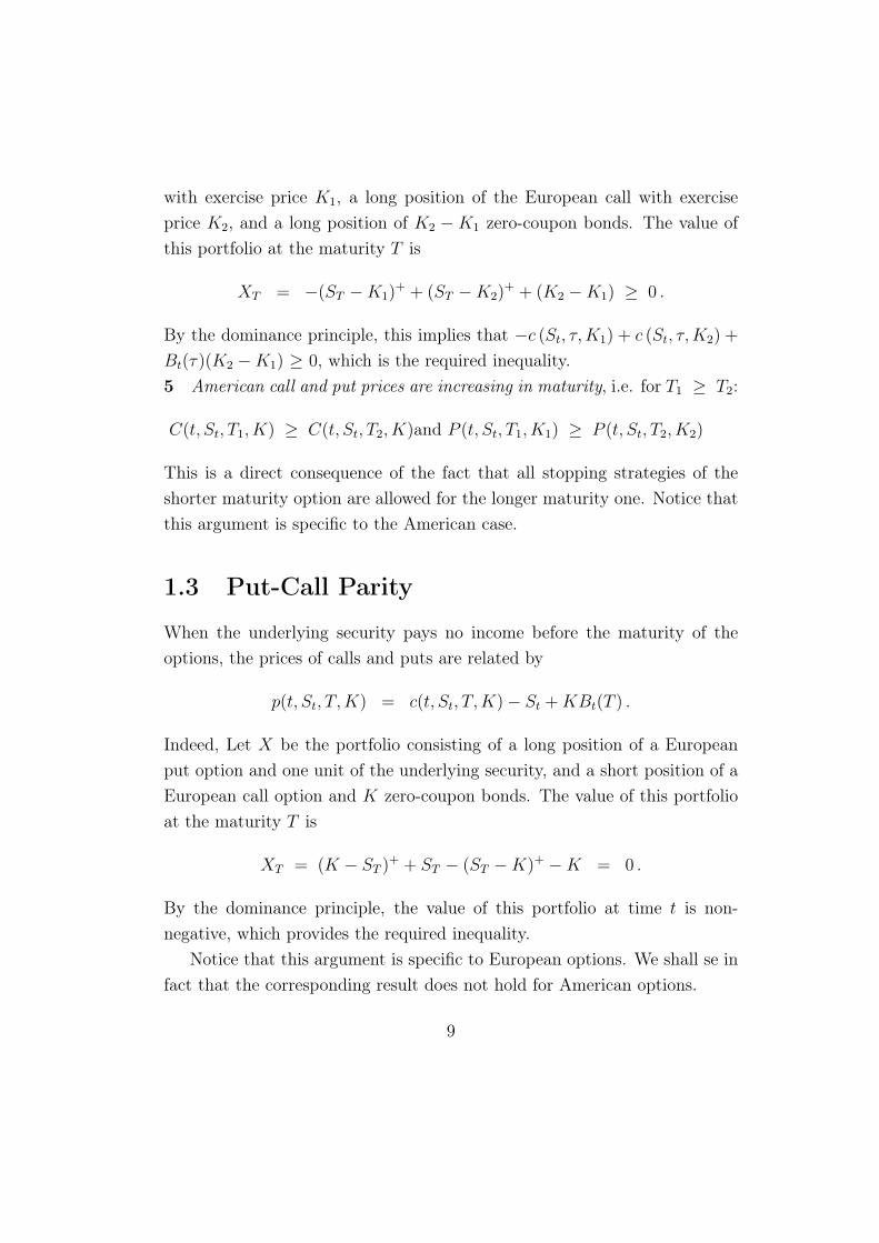
5 American call and put prices are increasing in maturity, i.e. for T1 ≥ T2:
C(t, St, T1, K) ≥ C(t, St, T2, K)and P (t, St, T1, K1) ≥ P (t, St, T2, K2)
This is a direct consequence of the fact that all stopping strategies of the
shorter maturity option are allowed for the longer maturity one. Notice that
this argument is specific to the American case.
1.3 Put-Call Parity
When the underlying security pays no income before the maturity of the
options, the prices of calls and puts are related by
p(t, St, T,K) = c(t, St, T,K)− St +KBt(T ) .
Indeed, Let X be the portfolio consisting of a long position of a European
put option and one unit of the underlying security, and a short position of a
European call option and K zero-coupon bonds. The value of this portfolio
at the maturity T is
XT = (K − ST )+ + ST − (ST −K)+ −K = 0 .
By the dominance principle, the value of this portfolio at time t is non-
negative, which provides the required inequality.
Notice that this argument is specific to European options. We shall se in
fact that the corresponding result does not hold for American options.
9

Finally, if the underlying asset pays out some dividends then, the above
argument breaks down because one should account for the dividends received
by holding the underlying asset S. If we assume that the dividends are known
in advance, i.e. non-random, then it is an easy exercise to adapt the put-call
parity to this context. However, id the dividends are subject to uncertainty
as in real life, there is no direct way to adapt the put-call parity.
1.4 Bounds on call prices and early exercise of
American calls
1 From the monotonicity of American calls in terms of the exercise price,
we see that
c(St, τ,K) ≤ C(St, τ,K) ≤ St
• When the underlying security pays no dividends before maturity, we have
the following lower bound on call options prices:
C(t, St, T,K) ≥ c(t, St, T,K) ≥ (St −KBt(T ))+ .
Indeed, consider the portfolio X consisting of a long position of a European
call, a long position of K T−maturity zero-coupon bonds, and a short po-
sition of one share of the underlying security. The required result follows
from the observation that the final value at the maturity of the portfolio is
non-negative, and the application of the dominance principle.
2 Assume that interest rates are positive. Then, an American call on a
security that pays no dividend before the maturity of the call will never be
exercised early.
Indeed, let u be an arbitrary instant in [t, T ),
- the American call pays Su −K if exercised at time u,
- but Su −K < S −KBu(T ) because interest rates are positive.
- Since C(Su, u,K) ≥ Su − KBu(T ), by the lower bound, the American
10

option is always worth more than its exercise value, so early exercise is never
optimal.
3 Assume that the security price takes values as close as possible to zero.
Then, early exercise of American put options may be optimal before maturity.
Suppose the security price at some time u falls so deeply that Su <
K −KBu(T ).
- Observe that the maximum value that the American put can deliver when
if exercised at maturity is K.
- The immediate exercise value at time u is K − Su > K − [K −KBu(T )] =
KBu(T ) ≡ the discounted value of the maximum amount that the put could
pay if held to maturity,
Hence, in this case waiting until maturity to exercise is never optimal.
1.5 Risk effect on options prices
1 The value of a portfolio of European/american call/put options, with com-
mon strike and maturity, always exceeds the value of the corresponding basket
option.
Indeed, let S1, . . . , Sn be the prices of n security, and consider the portfolio
composition λ1, . . . , λn ≥ 0. By sublinearity of the maximum,
n∑
i=1
λi max
Siu −K, 0
≥ max
n∑
i=1
λiSiu −K, 0
i.e. if the portfolio of options is exercised on the optimal exercise date of
the option on the portfolio, the payoff on the former is never less than that
on the latter. By the dominance principle, this shows that the portfolio of
options is more maluable than the corresponding basket option.
2 For a security with spot price St and price at maturity ST , we denote its
return by
Rt(T ) :=ST
St
.
11

Definition Let Rit(T ), i = 1, 2 be the return of two securities. We say that
security 2 is more risky than security 1 if
R2t (T ) = R1
t (T ) + ε where E[
ε|R1t (T )
]
= 0 .
As a consequence, if security 2 is more risky than security 1, the above
definition implies that
Var[
R2t (T )
]
= Var[
R1t (T )
]
+ Var[ε] + 2Cov[R1t (T ), ε]
= Var[
R1t (T )
]
+ Var[ε] ≥ Var[
R1t (T )
]
3 We now assume that the pricing functional is continuous in some sense
to be precised below, and we show that the value of an European/American
call/put is increasing in its riskiness.
To see this, let R := Rt(T ) be the return of the security, and consider the
set of riskier securities with returns Ri := Rit(T ) defined by
Ri = R + εi where εi are iid and E [εi|R] = 0 .
Let C i(t, St, T,K) be the price of the American call option with payoff
(StRi −K)
+, and Cn(t, St, T,K) be the price of the basket option defined
by the payoff(
1n
∑ni=1 StR
i −K)+
=(
ST + 1n
∑ni=1 εi −K
)+.
We have previously seen that the portfolio of options with common ma-
turity and strike is worth more than the corresponding basket option:
C1(t, St, T,K) =1
n
n∑
i=1
C i(t, St, T,K) ≥ Cn(t, St, T,K).
Observe that the final payoff of the basket option Cn(T, ST , T,K)−→ (ST −K)+
a.s. as n→ ∞ by the law of large numbers. Then assuming that the pricing
functional is continuous, it follows that Cn(t, St, T,K) −→ C(t, St, T,K),
and therefore: that
C1(t, St, T,K) ≥ C(t, St, T,K) .
Notice that the result holds due to the convexity of European/American call/put
options payoffs.
12

1.6 Some popular examples of contingent claims
Example 1.1 (Basket call and put options) Given a subset I of indices in
1, . . . , n and a family of positive coefficients (ai)i∈I , the payoff of a Basket
call (resp. put) option is defined by
B =
(
∑
i∈IaiS
iT −K
)+
resp.
(
K −∑
i∈IaiS
iT
)+
.
♦
Example 1.2 (Option on a non-tradable underlying variable) Let Ut(ω) be
the time t realization of some observable state variable. Then the payoff of
a call (resp. put) option on U is defined by
B = (UT −K)+ resp. (K − UT )+ .
For instance, a Temperature call option corresponds to the case where Ut is
the temperature at time t observed at some location (defined in the contract).
Example 1.3 (Asian option)An Asian call option on the asset Si with ma-
turity T > 0 and strike K > 0 is defined by the payoff at maturity:
(
Si
T −K)+
,
where Si
T is the average price process on the time period [0, T ]. With this
definition, there is still choice for the type of Asian option in hand. One can
define Si
T to be the arithmetic mean over of given finite set of dates (outlined
in the contract), or the continuous arithmetic mean...
Example 1.4 (Barrier call options) Let B,K > 0 be two given parameters,
and T > 0 given maturity. There are four types of barrier call options on the
asset Si with stike K, barrier B and maturity T :
• When B > S0:
13

– an Up and Out Call option is defined by the payoff at the maturity
T :
UOCT = (ST −K)+1max[0,T ] St≤B.
The payoff is that of a European call option if the price process of
the underlying asset never reaches the barrier B before maturity.
Otherwise it is zero (the contract knocks out).
– an Up and In Call option is defined by the payoff at the maturity
T :
UICT = (ST −K)+1max[0,T ] St>B.
The payoff is that of a European call option if the price process of
the underlying asset crosses the barrier B before maturity. Oth-
erwise it is zero (the contract knocks out). Clearly,
UOCT +UICT = CT
is the payoff of the corresponding European call option.
• When B < S0:
– an Down and Out Call option is defined by the payoff at the ma-
turity T :
DOCT = (ST −K)+1min[0,T ] St>B.
The payoff is that of a European call option if the price process of
the underlying asset never reaches the barrier B before maturity.
Otherwise it is zero (the contract knocks out).
– an Down and In Call option is defined by the payoff at the matu-
rity T :
DICT = (ST −K)+1min[0,T ] St≤B.
14

The payoff is that of a European call option if the price process of
the underlying asset crosses the barrier B before maturity. Oth-
erwise it is zero. Clearly,
DOCT +DICT = CT
is the payoff of the corresponding European call option.
♦
Example 1.5 (Barrier put options) Replace calls by puts in the previous
example
15

Chapter 2
The finite probability one-period
model
2.1 The model
In this chapter, we consider a simple one-period financial market model with
d + 1 assets and two dates: t = 0 and t = 1. The randomness in the model
is represented by a finite space of the states of nature Ω = ω1, . . . , ωKwhich correspond to scenarios of market evolution between t = 0 and t = 1,
with σ-field F containing all subsets of Ω and associated probabilities P =
p1, . . . , pK which are supposed to be all positive. The prices of assets at
time t are denoted by (Sit)
di=0. The asset S0 represents the risk-free bank
account with deterministic evolution: S01 = 1 and S0
1 = 1 + R, where R is
the one-period interest rate, known at time t = 0. The other assets are risky:
their prices at time 1 are only revealed at t = 1.
A portfolio strategy θ ∈ Rd+1, is a vector giving the number of units
of each asset to be held in the portfolio between date 0 and date 1. The
portfolio value Xt is given by
Xt =d∑
i=0
θiSit .
16

Sometimes we will also use the notation Xθt to emphasize that the portfolio
is constructed using the strategy θ.
The gain of a portfolio strategy is defined by
G = X1 −X0 =d∑
i=0
θi∆Si, with ∆Si = Si1 − Si
0.
It is convenient to express the prices of all assets in the units of the risk-free
asset, or, in other words, choose the bank account as numéraire. We therefore
introduce discounted prices
Sit :=
Sit
S0t
and the discounted portfolio value
Xt =Xt
S0t
= θ0 +d∑
i=1
θiSit
The discoutned gain of the portfolio strategy does not depend on the number
of units of the risk-free asset in the portfolio:
G = X1 − X0 =d∑
i=1
θi∆Si.
Example 2.6 Let Ω = (ω1, ω2, ω3, ω4) with associated probabilities P = (0.3,
0.3, 0.2, 0.2) and R = 0.25. Assume that S1 is a stock whose price equals
1 at time t = 0, and takes values (0.5, 1, 1.5, 2) in the states (ω1, ω2, ω3, ω4)
respectively. Finally, let S2 be a call option on S1 with strike K = 1, which
costs 0.3 at time t = 0 and takes values (0, 0, 0.5, 1) in the respective states
of nature. It is convenient to represent this market using a table (see table
2.1).
We consider a strategy with zero initial cost, which consists in short-selling
one unit of stock, buying one call option on this stock (to limit the losses) and
placing the remaining funds in a bank. We therefore have θ = (0.7,−1, 1)
and
G =7
8− S1
1 + S21 =
3
8in ω1
−1
8in ω1, ω2, ω3.
17
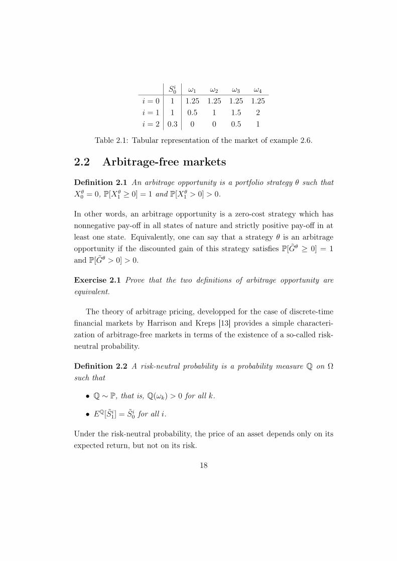
Si0 ω1 ω2 ω3 ω4
i = 0 1 1.25 1.25 1.25 1.25
i = 1 1 0.5 1 1.5 2
i = 2 0.3 0 0 0.5 1
Table 2.1: Tabular representation of the market of example 2.6.
2.2 Arbitrage-free markets
Definition 2.1 An arbitrage opportunity is a portfolio strategy θ such that
Xθ0 = 0, P[Xθ
1 ≥ 0] = 1 and P[Xθ1 > 0] > 0.
In other words, an arbitrage opportunity is a zero-cost strategy which has
nonnegative pay-off in all states of nature and strictly positive pay-off in at
least one state. Equivalently, one can say that a strategy θ is an arbitrage
opportunity if the discounted gain of this strategy satisfies P[Gθ ≥ 0] = 1
and P[Gθ > 0] > 0.
Exercise 2.1 Prove that the two definitions of arbitrage opportunity are
equivalent.
The theory of arbitrage pricing, developped for the case of discrete-time
financial markets by Harrison and Kreps [13] provides a simple characteri-
zation of arbitrage-free markets in terms of the existence of a so-called risk-
neutral probability.
Definition 2.2 A risk-neutral probability is a probability measure Q on Ω
such that
• Q ∼ P, that is, Q(ωk) > 0 for all k.
• EQ[Si1] = Si
0 for all i.
Under the risk-neutral probability, the price of an asset depends only on its
expected return, but not on its risk.
18
Theorem 2.1 A financial market admits no arbitrage opportunity if and
only if there exists at least one risk-neutral probability.
Proof. The if part. Let Q be a risk-neutral probability and assume that θ
is an arbitrage opportunity. Then, since EQ[Gθ] = 0, Gθ = 0 in all states of
nature and we have a contradiction with P[Gθ > 0] > 0.
The only if part. Suppose that the market is arbitrage-free, and let Q be
the set of all probability measures on Ω which assign nonzero probability to
every state:
Q = q ∈ RK : qi > 0 ∀i,K∑
i=1
qi = 1.
Further, let C be the d-dimensional set of all expectations of (∆Si)di=1 under
probabilities in Q:
C = EQ[∆S]|Q ∈ Q.
C is clearly a convex set, and to prove the existence of a risk-neutral proba-
bility it is sufficient to show that 0 ∈ C. Suppose on the contrary that 0 /∈ C.
Then by the separating hyperplane theorem [23] there exists H ∈ Rd such
that HTx ≥ 0 for all x ∈ C and Hx0 > 0 for some x0 ∈ C. Let θ = (H0, H)
with H0 arbitrary. For this strategy therefore EQ[Gθ] ≥ 0 for all Q ∈ Q and
EQ[Gθ] > 0 for some Q ∈ Q.
Suppose that Gθ(ωi) < 0 for some ωi ∈ Ω. Taking Qε =εK+(1−ε)1ωi
we
see that EQε [Gθ] < 0 for ε sufficiently small, which is a contradiction with
the above. Therefore, Gθ ≥ 0 in all states of nature, and Gθ > 0 in at least
one state: θ is an arbitrage opportunity. Since we have supposed that the
market is arbitrage free, this is a contradiction, and therefore we conclude
that 0 ∈ C and there exists at least one risk-neutral probability. ♦
Example 2.7 Let us look for a risk-neutral probability in the market of ex-
19
ample 2.6. We need to solve the system of equations
− 3
5q1 −
1
5q2 +
1
5q3 +
3
5q4 = 0
− 3
10q1 −
3
10q2 +
1
10q3 +
1
2q4 = 0
q1 + q2 + q3 + q4 = 1.
This system admits an infinity of positive solutions of the form
(q1, q2, q3, q4) =
(
1
4, q,
3
4− 2q, q
)
, q ∈(
0,3
8
)
.
The market of example 2.6 is therefore arbitrage-free.
Assume now that we add an additional asset to the market of example
2.6, which is a put option with strike 32, quoted at the price of 0.2 at t = 0.
We then need to add another equation to the above system, and the only
remaining solution is(
14, 0, 3
4, 0)
, which is not a risk-neutral probability. This
means that the enlarged market is not arbitrage-free. To find this opportunity
we need to construct a portfolio which only pays off in states ω2 and ω4. For
example, the strategy consisting in the purchase of a stock funded from a bank
account and simultaneous sale of a put option is an arbitrage opportunity.
2.3 Complete markets and pricing of attainable
claims
In this and the following section we assume that the market is arbitrage-free
and hence there exists a risk-neutral probability Q.
Definition 2.3 A contingent claim B is a random variable on (Ω,F ,P).
In our simple setting, a random variable is simply a vector of values taken
in different states of nature, and the contingent claim is therefore identified
with the vector of its pay-off valules in different states.
20

A contingent claim B is said to be attainable if there exists a strategy θ
such that B = Xθ1 . By the absence of arbitrage, the price of the contingent
claim at time 0 must then be given by p(B) = Xθ0 . Indeed, if the contingent
claim is quoted at a price p′ < p(B), then a strategy which consists in (i)
buying the contingent claim at t = 0; (ii) selling the portfolio Xθ, has a zero
terminal pay-off and generates an immediate profit of p(B)− p′. Similarly, if
the quoted price is greter than p(B), an arbitrage strategy can be constructed.
Since, under a risk-neutral probability Q, X0 = EQ[V1], we have the
following result:
Proposition 2.1 The fair price p(B) of an attainable contingent claim sat-
isfies
p(B) = EQ[B] = EQ
[
B
S01
]
,
where Q is any risk-neutral probability in the market.
Example 2.8 In the market of example 2.6, a put option with strike K = 1
is attainable (using the put-call parity) and one can check that its expected
discounted pay-off is equal to 110
under all the risk-neutral probabilities in this
market. The put option with strike K = 32
is not attainable.
Definition 2.4 A market is said to be complete if every contingent claim is
attainable.
Let A be the pay-off matrix: Aik = Si1(ωk). The contingent claim B is
attainable if the equation θTA = B has a solution θ ∈ Rd+1. Every contingent
claim is attainable if θTA = B has a solution for every B ∈ RK , which is
the case if A has K linearly independent lines. This means that for a market
to be complete, the number of assets (including the risk-free asset) must be
greater or equal to the number of states of nature.
Example 2.9 If the market of example 2.6 is enlarged with a put option with
strike K = 32, it becomes complete (four linearly independent assets). If it
is enlarged with a put option with strike K = 1, it remains incomplete (four
assets but not linearly independent).
21

Theorem 2.2 An arbitrage-free market is complete if and only if the risk-
neutral probability is unique.
Proof. Suppose that the market is complete. Then the prices of the con-
tingent claims of the form 1ωkfor k = 1, . . . , K are uniquely defined and for
every risk-neutral probability Q we have
Q(ωk) = S01p(1ωi
).
Suppose that the risk-neutral probability Q is unique. We will show that
the pay-off matrix A has K linearly independent lines. If this is not the case,
there exists z ∈ RK with z 6= 0 and Az = 0. Then for ε sufficiently small,
Q+ εz is a risk-neutral probability different from Q. ♦
2.4 Asset pricing in incomplete markets
In incomplete markets, the fair price of some contingent claims is not unique,
but one can nevertheless compute bounds on their prices: the upper and lower
superhedging price, defined by
p+(B) = infp(C)|C attainable, C ≥ B,p−(B) = supp(C)|C attainable, C ≤ B.
In our finite-space model, we actually have
p+(B) = minp(C)|C attainable, C ≥ B,p−(B) = maxp(C)|C attainable, C ≤ B.
For example, in the case of p+, we can always restrict the set of attainable
claims over which we minimize to those satisfying C(ωi)Q(ωi) ≤ maxiB(ωi)
(where Q is any risk-neutral measure). Since the latter set is compact, the
inf is attained.
If the claim B is attainable, p+(B) = p−(B) but for genuinely inattainable
claims p−(B) < p(B) < p+(B) because equality would create arbitrage.
22

Theorem 2.3 In an arbitrage-free market, the upper and lower superhedging
prices are given by
p−(B) = infQ∈QRN
EQ[B]
p+(B) = supQ∈QRN
EQ[B],
where QRN is the set of all risk-neutral probabilities.
Proof. Assume first that p+(B) < supQEQ[B]. Then there exists Q ∈ QRN
with p+(B) < EQ[B] and an attainable claim C with p(C) < EQ[B] and C ≥B. Then EQ[C] < EQ[B] which is in contradiction with C ≥ B. Therefore
p+(B) ≥ supQEQ[B]. Similarly, we can show that p−(B) ≤ infQE
Q[B].
Assume now that p−(B) < infQEQ[B] and consider an extended market
where B is quoted at price p(B) with p−(B) < p(B) < infQEQ[B]. By
theorem 2.1, in this market there exists an arbitrage opportunity, which will
be denoted by (θ, θ′), where θ′ 6= 0 is the coefficient in front of B. If θ′ > 0
then B dominates the attainable portfolio − 1θ′θS, whose price is equal to
p(B) (by definition of the arbitrage opportunity) and hence greater than
p−(B), which gives a contradiction.
If θ′ < 0 then B is dominated by the attainable portfolio − 1θ′θS whose
price is equal to p(B). Therefore, p+(B) < infQEQ[B], which gives a contra-
diction with the first part of the proof.
Therefore, we conclude that p−(B) ≥ infQEQ[B] and in the same way we
can show that p+(B) ≤ supQEQ[B]. ♦
Example 2.10 Let us compute the arbitrage bounds for a put option with
strike K = 32
in example 2.6. The set EQ[B]|Q ∈ QRN coincides with
15+ 2
5q|0 < q < 3
8, and the bounds are therefore 1
5< p(B) < 7
20.
23

2.5 Portfolio optimization and equilibrium as-
set pricing
In this section, we consider the problem of an economic agent who disposes of
w euros at date t = 0 and wants to invest them optimally using the available
assets. Whereas the price of a contingent claim in a complete arbitrage-free
market is uniquely determined, the optimal investment policy depends on
the preferences of the agent: some agens will choose riskier portfolios than
others.
To measure the preferences of an agent, we introduce the utility function:
a function u : R → R or u : [0,∞) → R, which is strictly increasing and
strictly concave. The agent prefers holding portfolio X at date t = 1 to
holding the portfolio Y if and only if E[u(X)] ≥ E[u(Y )]. The fact that
u is increasing means that X is always preferred to Y if X ≥ Y , and the
concavity implies (via Jensen’s inequality) that E[X] is always preferred to
X. Since increasing linear transformations of the utility function do not
change the structure of preferences, the utility function is only defined up to
such transformations.
For a random financial flow X, the certainty equivalent of X is the con-
stant cX ∈ R such that u(cX) = E[u(X)]. The risk premium is the differ-
ence between the expected value of X and its certainty equivalent: ρ(X) =
E[X]− cX . Let m = E[X]. Then u(cX) = u(m− ρ) =≈ u(m)− u′(m)ρ. On
the other hand, u(cX) = E[u(X)] ≈ u(m) + 12u′′(m)Var(X). Therefore,
ρ ≈ α(m)Var(X)
2,
where α(x) = −u′′(x)u′(x)
is called the absolute risk aversion coefficient at the
level x.
Examples of utility functions Setting α(x) = α for all x, we obtain the
constant absolute risk aversion (CARA) utility defined for x ∈ R:
(− log u′)′ = α ⇒ u′ = ce−αx ⇒ u(x) = 1− e−αx.
24

Setting α = 1−γx
for γ ∈ [0, 1) leads to hyperbolic absolute risk aversion
(HARA) utility function, defined for x ∈ [0,∞), which models the situation
where the agent’s risk aversion decays with increasing wealth. We get:
(− log u′)′ =1− γ
x⇒ u′ = Cxγ−1.
If γ = 0, this leads to the logarithmic utility u(x) = log x, and the case γ > 0
corresponds to power utility u(x) = xγ
γ. One checks easily that
limγ→0
xγ
γ= log x.
2.5.1 The portfolio optimization problem
In this section, we are interested in the following problem:
maxθE[u(Xθ
1 )] (2.1)
subject to the constraint Xθ0 = w, called the budget constraint. First, let us
observe that if the market is not arbitrage-free, this problem does not have
a (finite) solution. Indeed, let θ be an optimal strategy with E[u(X θ1 )] < ∞
and θA be an arbitrage opportunity. Then the strategy θ + θA satisfies the
budget constraint and
E[u(X θ+θA1 )] > E[u(X θ
1 )],
which means that θ cannot be optimal. Therefore, from now on, we suppose
that the market is arbitrage-free. This means that there exits a risk-neutral
probability Q such that
EQ
[
Xθ1
(1 +R)
]
= w (2.2)
The budget constraint can therefore be replaced by the constraint (2.2), and
the utility maximization problem reduces to two independent problems:
25

• Maximize the utility over the set of all hedgeable claims subject to the
bugdet constraint:
maxX hedgeable
E[u(X)] subject to EQ[X] = (1 +R)w.
Let X be the claim which realizes the maximum.
• Find a trading strategy θ which replicates X. This is a problem that
we already know how to solve from previous sections.
At this point, two remarks are in order. First, if the market is complete, all
claims are hedgeable, and the first problem reduces to
maxE[u(X)] subject to EQ[X] = (1 +R)w. (2.3)
Secondly, exactly the same logic can be used to solve the portfolio optimiza-
tion problem in a multiperiod discrete-time model.
In view of the above discussion, from now on we concentrate on the prob-
lem (2.3), but without necessarily supposing that the market is complete. If
it is, this problem gives us an immediate solution to the portfolio optimiza-
tion problem. In the incomplete market case, it will allow us to understand
the optimal contingent claim profiles and explain the demand for derivative
products in financial markets. The problem of finding an optimal portfolio in
an incomplete market is more difficult and out of scope of this introductory
course.
2.5.2 Finding the optimal contingent claim
In this section, in addition to what was assumed before, we suppose that
the utility function u satisfies one of the two sets of conditions (called Inada
conditions):
(A1) u : R → R, is continuously differentiable on R, and satisfies limx→∞ u′(x) =
0 and limx→−∞ u′(x) = +∞ (the typical example is exponential utility).
26

(A2) u : [0,∞) → R, is continuously differentiable on (0,∞), and satisfies
limx→∞ u′(x) = 0 and limx→0 u′(x) = +∞ (the typical example is power
utility).
We consider a possibly incomplete arbitrage-free financial market with K
states of nature and associated probabilities (pi)Ki=1. Let Q = (qi)
Ki=1 be a
risk-neutral probability. The problem (2.3) becomes
maxx∈RK
K∑
i=1
piu(xi) subject toK∑
i=1
qixi = w(1 +R).
To solve it, we construct the Lagrangian:
L(x1, . . . , xK , λ) =K∑
i=1
piu(xi)− λ
K∑
i=1
xiqi − w(1 +R)
The first order conditions are
piu′(xi) = λqi.
This gives us a potential candidate for the optimal claim:
xi = (u′)−1
(
λqipi
)
:= I
(
λqipi
)
,
which makes sense as long as λ > 0 due to the assumptions in the beginning
of this section. The value of λ is found from the budget equation:
K∑
i=1
qiI
(
λqipi
)
= w(1 +R) (2.4)
The function
f(λ) =K∑
i=1
qiI
(
λqipi
)
is strictly decreasing and satisfies
limλ→0
f(λ) = +∞ and limλ→∞
f(λ) = −∞ under (A1)
limλ→0
f(λ) = +∞ and limλ→∞
f(λ) = 0 under (A2)
27

Therefore, under (A1), for every initial wealth w ∈ R there exists a solution
λ∗ > 0 of equation (2.4), and under (A2), such a solution exists for every
positive initial wealth w > 0. The optimal claim is then given by
x∗i = I
(
λ∗qipi
)
or X∗ = I(λ∗Z) with Z :=dQ
dP.
To show that X∗ is indeed the unique optimizer of the constrained problem
(2.3), assume that X ′ = (x′1, . . . , x′k) is another solution, different from X∗.
We then have:
K∑
i=1
piu(x′i) = L(x′1, . . . , x
′K , λ
∗) < L(x∗1, . . . , x∗K , λ
∗) =K∑
i=1
piu(x∗i ),
where the first equality holds because X ′ satisfies the budget equation, the
inequality is due to the strict concavity of L and the last equality follows
from the budget equation for X∗.
Example: exponential utility Let u(x) = 1− e−αx. Then
I(z) = − 1
αlog( z
α
)
and the budget equation can be solved explicitly:
EQ
[
− 1
αlog
(
λ∗Z
α
)]
= w(1 +R)
⇒ X∗ = w(1 +R) +1
α
EQ[logZ]− logZ
Therefore, in the exponential utility framework, every investor will want to
hold a share of the same risky claim with pay-off M =
EQ[logZ]− logZ
.
The amount to buy depends on the risk aversion of a particular investor,
but the claim itself is the same for all investors. Therefore, the aggregate
portfolio of all investors will be proportional to M , and we recover the mutual
fund theorem. Note also that if Q 6= P, by Jensen’s inequality,
EP[M ] = EP[(Z − 1) logZ] > 0
which means that the agents are rewarded for the risk they take.
28

2.5.3 Equilibrium asset pricing
In this section, our aim is to understand, how asset prices can be determined
endogeneously via a supply-demand equilibrium among market participants.
We suppose that the market consists of a finite set A of economic agents with
utility functions (ua)a∈A and initial endowments with pay-offs (Wa)a∈A. The
sum of all endowments M :=∑
a∈AWa is the market portfolio, that is, the
aggregate portfolio of all assets available for trading. A feasible allocation
(Xa)a∈A is a set of contingent claims satisfying the market clearing condition:
∑
a∈AXa =M.
The prices in the market will be determined via a pricing density φ: a random
variable φ > 0 satisfying E[φ] = 1. The price of a contingent claim X is
p(X) = E[
φX1+R
]
.
A microeconomic or Arrow-Debreu equilibrium is a pricing density φ∗ and
a feasible allocation (X∗a)a∈A, such that for every a ∈ A, Xa solves the utility
maximization problem for agent a subject to the budget constraint defined
by the pricing rule φ∗: E[φ∗Xa] = E[φ∗Wa].
In these introductory lecture notes we consider the simplest case where
all agents have an exponential utility function: ua(x) = 1− e−αax. Let φ be
a pricing density. Then the optimal allocation for agent a has the form
Xa = E[φWa] +1
αa
E[φ log φ]− log φ ,
and the market clearing condition becomes
M = E[φM ] +1
αE[φ log φ]− log φ
where we set 1α:=∑
a∈A1αa
. This implies that equilibrium pricing rule is
necessarily of the form
φ∗ =e−αM
E[e−αM ].
29

with this pricing rule, the optimal allocation for each agent
X∗a = E[φ∗Wa] +
α
αa
(M − E[φ∗M ])
evidently satisfies the market clearing condition. The couple (φ∗, X∗) is then
the unique equilibrium in this market. In equilibrium, the agents hold linear
shares of the market portfolio, which means that once again we recover the
mutual fund theorem.
30

Chapter 3
The finite probability multiperiod
model
3.1 The model
In this chapter we consider a discrete-time financial model with T peri-
ods. The randomness is once again represented by a finite probability space
(Ω,F ,P), but now we need to specify how the information is revealed through
time. This is described via the notion of filtration: an increasing sequence
of σ-fields F = (F0,F1, . . . ,FT ). The σ-field Ft contains all events which
are known at date t. We assume that F0 = (∅,Ω) and FT = F = 2Ω: no
information is available at date 0 and everything is known at date T .
The risky asset prices are modelled by d discrete-time stochastic processes
(Sit)
i=1,...,dt=0,1,...,T which are F-adapted, that is, Si
t is Ft measurable for every t.
This means that time-t prices of risky assets are revealed at date t.
The risk-free bank account process (S0t ) is defined by S0
0 = 1 and S0t =
S0t−1(1 + Rt), where Rt is the risk-free interest rate for the period between
t− 1 and t. The process (Rt)1≤t≤T is assumed to be F-predictable, meaning
that Rt is Ft−1-measurable for every t = 1, . . . , T : the risk-free rate for the
period is fixed in the beginning of the period.
31

Trading strategies The trading strategy is a d+1-dimensional stochastic
process (θit)i=0,...,dt=1,...,T , where θit represents the amount of i-th asset held in the
portfolio between dates ti−1 and ti. The trading strategies are also assumed
to be predictable: the portfolio composition for the period is known in the
beginning of the period.
For example, a constant strategy θit = θi0 corresponds to buying the assets
at t = 0 and holding them until t = T . In the fixed-mix strategy, one fixes the
proportions ω0, . . . , ωd of the total wealth to invest into different assets, and
at each date the portfolio is readjusted to maintain the same proportions.
Since the asset prices do not vary proportionnally, the amounts of assets will
be different at each date for this strategy.
The gain process of a strategy is the stochastic process describing the
change in the portfolio value due to the variation of the asset prices:
G0 = 0, Gt =t∑
s=1
d∑
i=0
θis∆Sis, ∆Si
t = Sit − Si
t−1.
Self-financing stategies The value of a portfolio may change throughout
time due to two factors:
• Variation of asset prices;
• Adding/withdrawal of funds during transactions.
A self-financing portfolio strategy is a strategy where no funds are added
to/withdrawn from the portfolio after the initial date, and the change in
portfolio value is therefore only due to variations of asset prices.
The portfolio value at date t just before the transaction can be written
asd∑
i=0
θitSit ,
and that after the transaction is given by
d∑
i=0
θi+1t Si
t .
32

For a self-financing strategy these two values are equal and the value of
portfolio at date t is defined uniquely by
Xt =d∑
i=0
θitSit = X0 +Gt.
Discounting Similarly to the one-period model, we define
Sit =
Sit
S0t
, Xt =Xt
S0t
= X0 + Gt,
where
Gt =t∑
s=1
d∑
i=1
θis∆Sit .
The discounting allows once again to eliminate all dependency of the gain
process on the risky asset.
3.2 Arbitrage-free markets
Definition 3.5 An arbitrage opportunity is a self-financing portfolio strategy
θ such that
Xθ0 = 0, P[Xθ
T ≥ 0] = 1 and P[XθT > 0] > 0.
Equivalently, an arbitrage opportunity is a strategy with P[GθT ≥ 0] = 1 and
P[GθT > 0] > 0. In multi-period models, in addition to static arbitrage op-
portunities, such as violation of the put-call parity, there may exist dynamic
arbitrage opportunities, which cannot be realized by buy-and-hold strategies.
Arbitrage-free multiperiod markets can be characterized via the existence
of a martingale probability, which is a generalization of the notion of risk-
neutral probability from the one-period setting.
Theorem 3.4 The T -period financial market is arbitrage-free if and only
if there exists a probability Q such that Q(ω) > 0 for all ω ∈ Ω and the
discounted prices of all assets are Q-martingales:
EQ[Sit+1|Ft] = Si
t , i = 0, . . . , d, t = 0, . . . , T − 1.
33

Proof. Let Q be a martingale probability. Then the discounted value (Xt)
of every self-financing portfolio is a Q-martingale, so that for every strategy
θ with Xθ0 = 0 we have EQ[Xθ
T ] = 0, which is in contradiction with V θT ≥ 0
in all states and V θT > 0 in at least one state.
Conversely, assume that the market is aribtrage-free. We consider a one-
period market with the same states of nature Ω as the original one, with
one risk-free asset evolving with zero interest rate, and with the risky assets
having pay-offs of the form
1At(Si
t − Sit−1) ∀t = 1, . . . , T, ∀i = 1, . . . , d, ∀At ∈ Ft−1,
and quoted all at zero price at the initial date. Since Ω is finite, there is only
a finite number of such risky assets. This number will be denoted by D. For
j = 1, . . . , D, we denote the pay-off of the j-th asset by 1A(j)(Si(j)t(j) − S
i(j)t(j)−1)
We claim that the new market is also arbitrage-free. Indeed, assume that
w ∈ RD+1 is an arbitrage strategy in this market. The discounted gain G
associated to this strategy can be written as
G =D∑
j=1
wj1A(j)(Si(j)t(j) − S
i(j)t(j)−1) =
T∑
s=1
d∑
i=1
D∑
j=1
wj1i(j)=i1t(j)=s1A(j)(Sis − Si
s−1)
=T∑
s=1
d∑
i=1
θis(Sis − Si
s−1),
where
θis =D∑
j=1
wj1i(j)=i1t(j)=s1A(j) ∈ Fs−1.
Therefore, G is the discounted gain of a self-financing strategy in the original
market, and since the original market is arbitrage free, it is not possible that
P [G ≥ 0] = 1 and P [G > 0] > 0.
From Theorem 2.1 we then know that there exists a probability Q on Ω
which satisfies Q(ω) > 0 for all ω ∈ Ω and
EQ[
1At(Si
t − Sit−1)
]
= 0
34

for all At ∈ Ft−1, which implies that
EQ[Sit |Ft−1] = Si
t−1,
and therefore Q is a martingale probability for the original market,
♦
3.3 Evaluation of contingent claims
A European contingent claim is a FT -measurable random variable, which
represents the pay-off of an option at time T . For example, a European
call option has pay-off B = (ST −K)+, where S is the price process of the
underlying asset; an Asian call option has pay-off B =(
1T
∑Tt=0 St −K
)+
.
A contingent claim B is said to be attainable or hedgeable if there exists a
self-financing strategy θ such that XθT = B. By arbitrage arguments, similar
to the ones used in the previous chapter, the price of B at any date t is then
given by pt(B) = Xθt . Since under any risk-neutral probability Q, Xθ
t is a
martingale, we obtain the following result:
Proposition 3.2 The fair price pt(B) of an attainable contingent claim at
date t satisfies
pt(B) = S0tE
Q
[
B
S0T
∣
∣Ft
]
,
where Q is any martingale probability.
The price of a non-attainable contingent claim is not uniquely defined, but
one can, as in the one-period model, establish arbitrage bounds for this price
in terms of the set of risk-neutral probabilities in the market:
infQ∈QM
S0tE
Q
[
B
S0T
∣
∣Ft
]
≤ pt(B) ≤ supQ∈QM
S0tE
Q
[
B
S0T
∣
∣Ft
]
,
where QRN is the set of all martingale probabilities.
35

3.4 Complete markets
As in the one-period model, a market is said to be complete if every contin-
gent claim is attainable. Moreover, the same characterization in terms of the
uniqueness of the martingale probability holds.
Theorem 3.5 An arbitrage-free market is complete if and only if the mar-
tingale probability is unique.
Proof. The only if part. Assume that the market is complete. This means
that every contingent claim is attainable and has a unique price, in particular
the claims S0T1ωi
for every i, which shows the uniqueness of the martingale
probability.
The if part. By way of contradiction, assume that there exists a non-
attainable contingent claim. We consider a one-period market with the same
states of nature Ω as the original one, with the one risk-free asset evolving
with zero interest rate, and with the risky assets having pay-offs of the form
1At(Si
t − Sit−1) ∀t = 1, . . . , T, ∀i = 1, . . . , d, ∀At ∈ Ft−1,
and quoted all at zero price at the initial date. Since Ω is finite, there is only
a finite number of such risky assets. In this one-period market there is also
a non-attainable claim, and by theorem 2.2, there exists a probability Q∗ on
Ω which is different from Q and satisfies
EQ∗
[
1At(Si
t − Sit−1)
]
= 0
for all At ∈ Ft−1, which implies that
EQ∗
[Sit |Ft−1] = Si
t−1,
and therefore Q∗ is a martingale probability for the original market, different
from Q. ♦
36

3.5 On discrete-time martingales
In this section, we recall some results from the theory of discrete-time mar-
tingales.
Definition 3.6 A F-adapted process M = Mt, t = 0, . . . , T is an (F,P)−supermartingale
(resp. (F,P)−submartingale) if Mt is P-integrable for every t and
E [Mt|Ft−1] ≤ (resp. ≥) Mt−1 for every t = 1, . . . , T .
A process M is an (F,P)−martingale if it is both an (F,P)−supermartingale
and an (F,P)−submartingale.
Example 3.11 LetM be an (F,P)−martingale and φ an F−adapted bounded
process. Then, the process Y defined by :
Y0 = 0 and Yt =t∑
k=1
φk−1(Mk −Mk−1) , t = 1, . . . , T
is an (F,P)−martingale.
This example allows to build a large family of (F,P)−martingales out of
some given (F,P)−martingale M . Notice however that the process φ needs
to satisfy a convenient restriction, namely φ has to be essentially bounded.
Without this restriction, we do not even have the guarantee that Y is inte-
grable, and we are led to the notion of local martingales ; see Definition 3.8
below.
Definition 3.7 An F−stopping time ν is a random variable with values in
0, . . . , T such that
ν = t ∈ Ft for every t = 0, . . . , T .
We shall denote by T the set of all F−stopping times.
37

Remark 3.1 An equivalent characterization of an F−stopping time is that
ν ≤ t ∈ Ft for every t = 0, . . . , T ,
(exercise !). This definition extends to the continuous-time setting.
Let Y = Yt, t = 0, . . . , T be an F-adapted process. The stopped process
Y ν at the F−stopping time ν is defined by :
Y νt := Yt∧ν for t = 0, . . . , T .
Exercise 3.2 Let Y be an F-adapted process and consider some F−stopping
time ν ∈ T .
1. Prove that the stopped process Y ν is F-adapted.
2. If Y is an (F,P)−martingale (resp. (F,P)−supermartingale), prove that
Y ν an (F,P)−martingale (resp. (F,P)−supermartingale).
For every stopping time ν, the available information at time ν is defined
by :
Fν := A ∈ F : A ∩ ν = t ∈ Ft for all t = 0, . . . , T .
We recall the following important result on stopped martingales.
Theorem 3.6 (Optional sampling, Doob). Let M be a martingale (resp.
supermartingale), and consider two stopping times ν, ν ∈ T with ν ≤ ν a.s.
Then :
E [Mν |Fν ] = Mν (resp. ≤ Mν) P− a.s.
Proof. We only prove this result for martingales ; the case of supermartin-
gales is treated similarly.
(i) We first show that E[MT |Fν ] =Mν for every ν ∈ T . Let A be an arbitrary
event set in Fν . Then, the event set A ∩ ν = t ∈ Ft and therefore :
E[
(MT −Mν)1A∩ν=t]
= E[
(MT −Mt)1A∩ν=t]
= 0
38

since M is a martingale. Summing up these inequalities, it follows that :
0 =T∑
t=0
E[
(MT −Mν)1A∩ν=t]
= E [(MT −Mν)1A] .
Since A is arbitrary in Fν , this proves that E[MT −Mν |Fν ] = 0.
(ii) By the second question of Exercise 3.2, the stopped process M ν is a
martingale. Then, by the above step (i), we see that :
E [Mν |Fν ] = E [M νT |Fν ] = M ν
ν = Mν
since ν ≤ ν. ♦
We next introduce the notion of local martingales.
Definition 3.8 A process M = Mt, t = 0, . . . , T is said to be a local
martingale if there exists a sequence of (F,P)−stopping times (τn)n such that
τn −→ ∞ P -a.s. and the stopped process M τn is an (F,P)−martingale for
every n.
Example 3.12 LetM be an (F,P)−martingale and φ an arbitrary F-adapted
process. Then, the process Y defined by :
Y0 := 0 and Yt =:t∑
k=1
φk−1(Mk −Mk−1) , t = 1, . . . , T
is a local martingale. To see this, consider the sequence of stopping times
τn := inf t : |φt| ≥ n ,
with the convention inf ∅ = ∞. Then, for every n ≥ 1,
Y τnt =
t∑
k=1
φk−1(Mk −Mk−1) where φt := φt1t<τn , t = 1, . . . , T .
Since φ is an F-measurable bounded process, we are reduced to the context
of Example 3.11, and the stopped process Y τn is an (F,P)−martingale.
39

The following result provides a sufficient condition in finite discrete time
for a local martingale to be a martingale.
Lemma 3.1 Let M = Mt, t = 0, . . . , T be an (F,P)−local martingale
with :
E[M−T ] < ∞ .
Then, M is an (F,P)−martingale.
Proof. Let (τn)n be a sequence of stopping times such that τn −→ ∞a.s. and the stopped process M τn is an (F,P)−martingale for every n. We
organize the proof into two steps.
1. We first prove that :
E[|Mt||Ft−1] <∞ and E[Mt|Ft−1] =Mt−1 P− a.s. 1 ≤ t ≤ T . (3.1)
Since τn is an (F,P)−stopping time, we deduce that the event set τn > t−1is Ft−1−measurable. Then :
E[|Mt||Ft−1] = E[|M τnt ||Ft−1] < ∞ P− a.s. on τn > t− 1 ,
where the last inequality follows from the fact that M τn is P−integrable. By
sending n to infinity, we deduce that E[|Mt||Ft−1] < ∞ P -a.s.
Similarly, using the martingale property of the stopped process M τn , we
see that :
E[Mt|Ft−1] = E[M τnt |Ft−1] = M τn
t−1 = Mt−1 on τn > t− 1 ,
which implies that E[Mt|Ft−1] =Mt−1 P -a.s. by sending n to infinity (Notice
that the condition E[M−T ] <∞ has not been used in this step).
2. It remains to prove that Mt is P−integrable for all t = 0, . . . , T .
By the second property of (3.1), together with the convexity of the function
x 7−→ x− and the Jensen inequality, we see that :
M−t ≤ E[M−
t+1|Ft] for every t = 0, . . . , T − 1 .
40

Then, E[M−t ] ≤ E[M−
t+1] ≤ . . . ≤ E[M−T ] <∞ by the condition of the lemma.
We next use Fatou’s lemma to obtain :
E[M+t ] = E
[
lim infn→∞
M+t∧τn
]
≤ lim infn→∞
E[
M+t∧τn]
= lim infn→∞
E[
Mt∧τn +M−t∧τn]
.
Recall that the stopped process M τn is an (F,P)−martingale. Then :
E[M+t ] ≤ M0 + lim inf
n→∞E[
M−t∧τn]
≤ M0 +T∑
t=0
E[M−t ] < ∞ .
♦
We next provide an example of a local martingale which fails to be a
martingale.
Example 3.13 Let (An)n≥1 be a measurable partition of Ω with P[An] =
2−n. Let (Zn)n≥1 be a sequence of random variables independent of An with
P[Zn = 1] = P[Zn = −1] = 1/2. Set
F0 := σ(An, n ≥ 1) and F1 := σ(An, Zn, n ≥ 1) ,
and consider the process
X0 := 0 and X1 := Y∞ = limn→∞
Yn where Yn :=∑
1≤p≤n
2pZp1Ap.
Clearly, X = X0, X1 is not an (F,P)−martingale as X1 = Y∞ is not in-
tegrable. We next show that X is an(F,P)−local martingale. Define the
sequence of stopping times :
τn := +∞ on ∪1≤p≤n Ap and τn := 0 on Ω \ (∪1≤p≤nAp) .
For every n, the stopped process Xτn is given by :
Xτn0 = 0 and Xτn
1 = Yn .
Since the random variable Yn is bounded and independent of F0, we easily
see that E[Yn|F0] = 0. Hence, Xτn is an (F,P)−martingale. ♦
41

Remark 3.2 In finite discrete-time, Lemma 3.1 provides an easy neces-
sary and sufficient condition for a local martingale to be a martingale (ne-
cessity is trivial). This condition does not extend to the contionuous-time
framework, as we will provide an example of a positive continuous-time (in-
tegrable) local martingale which fails to be a martingale. ♦
3.6 American contingent claims in complete fi-
nancial markets
3.6.1 Problem formulation
In the previous chapters, we have considered the so-called “European” con-
tingent claims which are defined by some payoff at some given maturity T .
For instance, a European call option on the asset S1 is defined by the
payoff (S1T − K)+ at time T . The buyer of such a contingent claim can
exercise the option at the maturity date T by buying the risky asset S1 at
the pre-fixed price K. Similarly, a European put option on the asset S1 is
defined by the payoff (K−S1T )
+ at time T , and the buyer of such a contingent
claim can exercise the option at the maturity date T by selling the risky asset
S1 at the pre-fixed price K.
Hence, the buyer of the European option decides whether to exercise or
not the option at the final time T . The latter restriction is dropped in the
case of American options, which allow the buyer to exercise the option at
any time before the maturity T . Consequently, an American call option is
defined by the process of payoffs (S1t −K)+, t = 1, . . . , T, i.e. the buyer of
this contingent claim receives the payoff (St −K)+ if he decides to exercise
the option at time t.
Similarly, an American put option allows the buyer to sell the risky asset
S1, for the price defined by the strike K, at any time before the maturity T .
Such an option is defined by the process of payoffs (K−St)+, t = 1, . . . , T,
i.e. the buyer of an American put option receives the payoff (K − St)+ if he
42

decides to exercise the option at time t.
This leads to the following concept of American contingent claims.
Definition 3.9 An American contingent claim is a process B = Bt, t =
1, . . . , T adapted to the filtration F.
The seller of an American contingent claim has to face the promised payoff
Bt at any time t before the maturity T , as the buyer can decide to exercise
his right. Then, the relevant super-hedging problem in this context is :
V a(B) := inf
x ∈ R : Xx,θt ≥ Bt, 1 ≤ t ≤ T a.s. for a θ ∈ A
. (3.2)
3.6.2 Decomposition of supermartingales
In the previous chapters, the concept of martingales played an important
role. In the setting of American contingent claim, we shall make use of the
notion of supermartingales.
Definition 3.10 Let Q be some given probability measure, and Y an F-
adapted process. We say that Y is a Q−supermartingale for the filtration F
if Yt is Q−integrable for all t ≤ T and
EQ[Yt|Fk] ≤ Yk for 0 ≤ k < t ≤ T .
It is immediately checked that we may formulate an equivalent definition
by taking k = t− 1. The analysis of supermartingales is usually reduced to
that of martingales thanks the following decomposition result.
Theorem 3.7 (Doob-Meyer). Let Q be a probability measure and Y a Q-
supermartingale for F. Then Y has the following unique decomposition :
Yt = Mt − At , t = 0, . . . , T ,
where M is a Q−martingale for F and A is a predictable non-decreasing
process with A0 = 0.
43

Proof. For t = 0, the only possible choice is M0 = Y0 since A0 = 0. Next,
we must have :
Yt+1 − Yt = Mt+1 −Mt − (At+1 − At) .
Since M has to be a martingale, this implies that :
−(At+1 − At) = EQ [Yt+1|Ft]− Yt , t = 0, . . . , T − 1 .
Since Y is a Q−supermartingale and A0 = 0, this defines a non-decreasing
process A. Then, the unique choice for the process M is :
M0 = Y0 and Mt+1 −Mt = Yt+1 − EQ[Yt+1|Ft] , t = 0, . . . , T − 1 .
Clearly, this process is a Q−martingale. ♦
3.6.3 The Snell envelope
Let B = Bt, t = 0 . . . , T be an F−adapted process (an American contingent
claim !) satisfying :
EQ
[
supt=0,...,T
|Bt|]
< ∞ ,
where Q is some given probability measure. In this paragraph, we study the
process Y defined by the backward induction
YT = BT and Yt = max
Bt,EQ[Yt+1|Ft]
, t = 0, . . . , T − 1 .
Exercise 3.3 Provide a financial interpretation of the process Y .
Proposition 3.3 The process Y is a Q−supermartingale. It is the smallest
Q−supermartingale which is larger than the process B.
Proof. The supermartingale property of Y together with the fact that
Y ≥ B follows immediately from the definition of Y . Let Y be a Q-
supermartingale larger than B, and let us show by induction that Yt ≥ Yt
for all t = 0, . . . , T Q−-a.s.
44

By definition, YT ≥ BT = YT . Suppose that Yt ≥ Yt. Since Y is a Q-
supermartingale, we have :
Yt−1 ≥ EQ[Yt|Ft−1] ≥ EQ[Yt|Ft−1] .
Since Y ≥ B, this implies that
Yt−1 ≥ max
Bt−1,EQ[Yt|Ft−1]
= Yt−1 .
♦
Definition 3.11 The process Y is called the Snell envelope of B for the
probability measure Q and the filtration F.
Let T denote the collection of all stopping times with values in 0, . . . , T.Our next result provides a representation of the Snell envelope in terms of
the underlying process B and the stopping times of T .
Proposition 3.4 The random variable
ν∗ := inft = 0, . . . , T : Yt = Bt
is a stopping time such that the stopped process Y ν∗ is a Q−martingale and
Y0 = supν∈T
EQ[Bν ] = EQ[Bν∗ ] .
Proof. (i) We first show that ν∗ defines a stopping time. Since YT = BT , the
random variable ν∗ takes values in 0, . . . , T. Clearly ν∗ = 0 = Y0 = B0∈ F0 and for t ≥ 1 :
ν∗ = t =(
∩t−1k=0Yk > Bk
)
∩ Yt = Bt ∈ Ft
since Y and B are both F−adapted.
(ii) We next prove that the stopped process Y ν∗ is a Q−martingale. By
definition of ν∗, we have :
Y ν∗
t+1 − Y ν∗
t = (Yt+1 − Yt)1ν∗≥t+1 .
45

By definition of the process Y , we have Yt > Bt and Yt = EQ[Yt+1|Ft] on
the event set ν∗ ≥ t + 1 (Ft-measurable as the complement of ν∗ ≤ t).Hence :
Y ν∗
t+1 − Y ν∗
t = (Yt+1 − EQ[Yt+1|Ft])1ν∗≥t+1 ,
and the required result is obtained by taking the expected values condition-
ally on Ft and using the fact that ν∗ ≥ t+ 1 ∈ Ft.
(iii) Since the stopped process Y ν∗ is a Q−martingale, we have :
Y0 = EQ[
Y ν∗
T
]
= EQ [YT∧ν∗ ] = EQ [Yν∗ ] = EQ [Bν∗ ] .
Moreover, for all ν ∈ T , the stopped process Y ν is a Q−supermartingale.
Therefore,
Y0 ≥ EQ[Y νT ] = EQ[Yν ] ≥ EQ[Bν ]
by definition of Y . This completes the proof of the proposition. ♦
3.6.4 Valuation of American contingent claims in a com-
plete market
In this section, we assume that the financial market satisfies the no-arbitrage
condition and is complete. By Theorems 3.4 and 3.5, we know that the set
of all equivalent martingale measures, or risk neutral probability measures,
is reduced to a singleton :
M(S) = P0 .
We consider an American contingent claim satisfying the integrability con-
dition
EP0
[
supt=0,...,T
|Bt|]
< ∞ , (3.3)
The next result expresses the super-replication problem for American con-
tingent claim (3.2) as an optimal stopping problem.
46

Theorem 3.8 Let B be an American contingent claim satisfying (3.3). Then,
V a(B) = supν∈T
EP0
[Bν ] = EP0
[Bν∗ ] ,
where ν∗ = inft = 0, . . . , T : Yt = Bt and Y is the Snell envelope of the
process B for the probability measure P0 and the filtration F.
Proof. (i) Let Y be the Snell envelope of the process B. This defines the
process Y by the usual relation Y := S0Y . As a P0-supermartingale, the
Snell envelope Y has the Doob-Meyer decomposition :
Yt = Mt − At , t = 0, . . . , T ,
where M is a P0−martingale and A a non-decreasing process with A0 =
0. Since the financial market is complete, the (European) contingent claim
defined by the random variable S0TMT is attainable, i.e. there exists a self-
financing portfolio strategy θ ∈ A such that :
MT = EP0
[MT ] +T−1∑
t=0
θt ·(
St+1 − St
)
= Y0 +T−1∑
t=0
θt ·(
St+1 − St
)
as A0 = 0. Since the process S is a P0-martingale, the process XY0,θ is a
P0-local martingale. Since XY0,θT = MT = YT +AT = BT +AT ≥ BT , we see
that (XY0,θT )− ≤ B−
T , so that (XY0,θT )− is P0-integrable by Condition (3.3). By
Lemma 3.1, this proves that :
Mt = XY0,θt = Y0 +
t−1∑
k=0
θk · (Sk+1 − Sk) , t = 1, . . . , T .
We have then found a self-financing portfolio strategy θ ∈ A such that :
XY0,θt = Y0 +
t−1∑
k=0
θk · (Sk+1 − Sk)
= Yt + At
≥ Yt
≥ Bt
47

for t = 1, . . . , T . By definition of V a, this shows that Y0 ≥ V a(B), and by
Proposition 3.4, we obtain the first inequality
V a(B) ≤ supν∈T
EP0[
Bν
]
= EP0
[Bν∗ ] .
It remains to show that the converse inequality holds. We claim that
V a(B) ≥ V (Bν) for all ν ∈ T . (3.4)
Then, since p(Bν) = EP0[Bν ] for all ν ∈ T , this provides the required in-
equality. To prove (3.4), we observe that
V a(B) ≥ V (Bν , ν) := inf
x ∈ R : ∃ θ ∈ A, Xx,θν ≥ Bν a.s.
for every ν ∈ T . We next check that V (Bν) = V (Bν , ν). For x > V (Bν , ν),
there exists a self-financing portfolio strategy θ ∈ A such that Xx,θν ≥ Bν a.s.
Consider the portfolio strategy
θt(ω) = θt(ω)1ν(ω)≤t .
Then, Xx,θT = Xx,θ
ν = Xx,θν ≥ Bν , which shows that x ≥ V (Bν). By the
arbitrariness of x > V (Bν , ν), this proves that V (Bν , ν) ≥ V (Bν).
Conversely, let x > V (Bν). Then, Xx,θT ≥ Bν a.s. for some self-financing port-
folio strategy θ ∈ A. Now observe that the process Xx,θ is a P0-martingale
since S is a P0-martingale and B−ν is P0−integrable. Consequently, by taking
expected values under P0 conditionally to Fν , it follows from the optional
sampling Theorem 3.6 that Xx,θν ≥ Bν a.s. Hence, x ≥ V (Bν , ν) and there-
fore V (Bν) ≥ V (Bν , ν). ♦
The previous proof also provides as a by-product the optimal super-
hedging strategy, as the perfect hedging strategy of the European contingent
claim Bν∗ .
We conclude this chapter by the following sufficient condition for an
American contingent claim to coincide with the corresponding European con-
tingent claim BT .
48

Corollary 3.1 Suppose that the process B is a P0-submartingale, i.e. Bk ≤EP0
[
Bt|Fk
]
for 0 ≤ k ≤ t ≤ T . Then :
V a(B) = V (BT ) = EP0
[BT ] .
Proof. By the optional sampling Theorem 3.6 :
V (BT ) = EP0
[BT ] ≤ supν∈T
EP0
[Bν ] = V a(BT ) ≤ supν∈T
EP0[
EQ[BT |Fν ]]
= EP0
[BT ]
by the tower property of conditional expectations. ♦
Remark 3.3 The last corollary applies to the case of American call options.
Let r be a constant interest rate, to simplify, and let us check that the process
e−rt(St − K)+, t = 0, . . . , T is a P0−submartingale. For 0 ≤ k < t ≤ T ,
we have :
EP0
[e−rt(St −K)+|Fk] ≥ EP0
[e−rt(St −K)|Fk]
= e−rkSk − e−rtK ≥ e−rk(Sk −K)
since S is a P0−martingale and r ≥ 0. Since EP0[(St − K)+|Fk] ≥ 0, this
provides :
EP0
[e−rt(St −K)+|Fk] ≥ e−rk(Sk −K)+ .
We may also obtain this inequality by the Jensen inequality.
From the previous remark, the no-arbitrage price of an American call
option is equal to that of the corresponding European call option, and it is
optimal to exercise the American option at the maturity T . This property
was obtained by a no-arbitrage argument without any model specification in
section 1.4.
Observe however that the corollary does not apply to American put op-
tions whenever the interest rate parameter r is strictly positive.
49

Chapter 4
The Cox-Ross-Rubinstein model
In this chapter we study the best-known mutiperiod discrete time model:
the binomial tree, or Cox-Ross-Rubinstein (CRR) model. Despite its sim-
plicity, this model is quite often used in practice, because it provides simple
algorithms for pricing exotic derivatives and can be considered as an approx-
imation to more complex continuous time models.
4.1 The one-period binomial model
We first study the simplest one-period financial market T = 1. Let Ω =
ωu, ωd, F the σ-algebra consisting of all subsets of Ω, and P a probability
measure on (Ω,F) such that 0 < P(ωu) < 1.
The financial market contains a non-risky asset with price process
S00 = 1 , S0
1(ωu) = S01(ωd) = er := 1 +R ,
and one risky asset (d = 1) with price process
S0 = s , S1(ωu) = su , S1(ωd) = sd ,
where s, r, u and d are given strictly positive parameters with u > d. Such
50

a financial market can be represented by the binomial tree :
time 0 time 1
Su
Risky asset S0 = s
Sd
Non-risky asset S00 = 1 1 +R
(i) The No-Arbitrage condition : By Theorem 2.1, the no-arbitrage condition
is equivalent to the existence of a probability measure Q, defined par qu =
Q(ωu) and qd = Q(ωd) = 1− qu, equivalent to P, i.e. 0 < qu < 1, such that
qusu
1 +R+ (1− qu)
sd
1 +R= s .
This linear equation admits a unique solution :
qu =1 +R− d
u− d,
and we directly check that 0 < qu < 1 if and only if :
u > 1 +R > d . (4.1)
In addition, we observe that the set of risk-neutral probabilities is reduced
to a singleton in the present setting and hence the market is complete.
(ii) Hedging contingent claims : A contingent claim is defined by its payoff
Bu := B(ωu) and Bd := B(ωd) at time 1.
The discounted wealth at time 1 of a portfolio with initial value x and
the quantity of risky asset equal to θ is given by :
Xx,θ1 = x+ θ(S1 − s) .
In this context , it turns out that there exists a pair (x0, θ0) such thatXx0,θ0
T =
B. Indeed, the equality Xx0,θ0
1 = B is a system of two (linear) equations with
51

two unknowns which can be solved straightforwardly :
x0 = quBu
1 +R+ (1− qu)
Bd
1 +R= EQ[B] and θ0 =
Bu −Bd
su− sd.
We also observe in our simple context that such a pair (x0, θ0) is unique.
Then x0 = EQ [Be−r] and (x0, θ0) is a perfect replication strategy for B, i.e.
Xx0,θ0
1 = B.
(iii) No arbitrage valuation : Let us denote by p(B) the market price of the
contingent claim contract. Under the no-arbitrage condition we have that
p(B) = EQ[
Be−r]
. (4.2)
Hence in the context of the simple binomial model, the no-arbitrage condi-
tion implies a unique valuation rule. This is the no-arbitrage price of the
contingent claim B.
In order to better understand this result, let us show directly this equality.
Suppose that the contingent claim B is available for trading at time 0. We
will now show that, under the no arbitrage condition, the price p(B) of the
contingent claim contract is necessarily given by p(B) = x0.
(iii-a) Indeed, suppose that p(B)< x0, and consider the following portfolio
strategy :
- at time 0, pay p(B) to buy the contingent claim, so as to receive the
payoff B at time 1,
- perform the self-financing strategy (−x0,−θ), this leads to paying −x0at time 0, and receiving −B at time 1
The initial capital needed to perform this portfolio strategy is p(B)−x0 < 0.
At time 1, the terminal wealth induced by the self-financing strategy exactly
compensates the payoff of the contingent claim. We have then built an
arbitrage opportunity in the financial market augmented with the contingent
claim contract, thus violating the no arbitrage condition on this enlarged
financial market.
(iii-b) If p(B) > x0, we consider the following portfolio strategy :
52

- at time 0, receive p(B) by selling the contingent claim, so as to pay the
payoff B at time 1,
- perform the self-financing strategy (x0, θ), this leads to paying x0 at
time 0, and receiving B at time 1
The initial capital needed to perform this portfolio strategy is −p(B)+ x0 <
0. At time 1, the terminal wealth induced by the self-financing strategy
exactly compensates the payoff of the contingent claim. This again defines an
arbitrage opportunity in the financial market augmented with the contingent
claim contract, thus violating the no arbitrage condition on this enlarged
financial market.
4.2 The dynamic CRR model
4.2.1 Description of the model
In this chapter, we consider a dynamic version of the binomial model intro-
duced in Section 4.1.
Let Ω = −1, 1N, and let F be the Borel σ-algebra on Ω. Let (Zk)k≥0 be
a sequence of independent random variables with distribution P[Zk = 1] =
P[Zk = −1] = 1/2. We shall see later that we may replace the value 1/2 by
any parameter in (0, 1), see Remark 4.6). We consider the standard filtration
F0 = ∅,F, Fk = σ(Z0, . . . , Zk) and Fn = F0, . . . ,Fn.Let T > 0 be some fixed finite horizon, and (bn, σn)n≥1 the sequence
defined by :
bn = bT
nand σn = σ
(
T
n
)1/2
,
where b and σ are two given strictly positive parameters.
Remark 4.4 All the results of this section hold true with a sequence (bn, σn)
satisfying :
nbn −→ bT and√nσn −→ σ
√T whenever n→ ∞ .
53
For n ≥ 1, we consider the price process of a single risky asset Sn = Snk ,
k = 0, . . . , n defined by :
Sn0 = s and Sn
k = s exp
(
kbn + σn
k∑
i=1
Zi
)
, k = 1, . . . , n .
The non-risky asset is defined by a constant interest rate parameter r, so
that the return from a unit investment in the bank during a period of length
T/n is
Rn := er(T/n) − 1 .
For each n ≥ 1, we have then defined a financial market with time step T/n.
In order to ensure that these financial markets satisfy the no-arbitrage
condition, we assume that :
dn < Rn − 1 < un where un = ebn+σn , dn = ebn−σn , n ≥ 1 .(4.3)
Exercise 4.4 Show that (4.3) is a necessary and sufficient conditon for the
financial markets of this section to satisfy the no-arbitrage condition.
Under this condition, there exists a unique risk neutral measure P0n defined
by :
P0n[Zi = 1] = qn :=
1 +Rn − dnun − dn
.
By Theorem 2.2, the above financial markets are complete.
4.2.2 Valuation and hedging of European options
In the rest of this chapter, we consider the contingent claims
Bn := g(Snn) where g(s) = (s−K)+ and K > 0 .
From the results of the previous chapters, the no-arbitrage price of this Eu-
ropean call option is :
pn(Bn) = e−rTEP0n[
(Snn −K)+
]
.
54

Under the probability measure P0n, the random variables (1+Zi)/2 are inde-
pendent and identically distributed as a Bernoulli with parameter qn. Then :
P0n
[
n∑
i=1
1 + Zi
2= j
]
= Cjnq
jn(1− qn)
n−j for j = 0, . . . , n .
This provides
pn(Bn) = e−rT
n∑
j=0
g(
sujndn−jn
)
Cjnq
jn(1− qn)
n−j .
By moving the time origin to kT/n, we obtain a trivial extension of the
problem with no-arbitrage price at time kT/n given by :
pnk(Bn) = e−r(1−(k/n))TEP0
n [Bn|Fk]
= e−r(1−(k/n))T
n−k∑
j=0
g(
Snku
jnd
n−k−jn
)
Cjn−kq
jn(1− qn)
n−k−j .
By the Tower property of conditional expectations, we observe that this
provides :
pnk(Bn) =
1
1 +Rn
EP0n[
pnk+1(Bn)|Fk
]
for k = 0, . . . , n− 1 . (4.4)
This formula shows that the no-arbitrage price of the European call option at
time 0 can be computed by a backward induction, avoiding the computation
of the combinatorial terms Cpn. Indeed pnn(B
n) = Bn is given and (4.4) reduces
to :
pnk(Bn) =
1
1 +Rn
[
qnpnk+1(B
n)un
+ (1− qn)pnk+1(B
n)dn
]
. (4.5)
Expression (4.4) reduces the multi-period valuation and hedging problem
into a sequence “local” one-period valuation and hedging problems. Indeed,
55

pnk(Bn) is the no-arbitrage price of the contingent claim pnk+1(B
n) :
date kT/n date (k + 1)T/n
unSnk
Risky asset Snk
dnSnk
pnk+1(Bn)
un
Contingent claim pnk(Bn)
pnk+1(Bn)
dn
Therefore, we can describe the (perfect) hedging strategy of the contingent
claim Bn by applying the one-period results of Section 4.1 :
θnk+1 =pnk+1(B
n)un
− pnk+1(Bn)
dn
unSnk − dnSn
k
, k = 0, . . . , n− 1 .
Remark 4.5 The hedging strategy is the finite differences approximation
(on the binomial tree) of the partial derivative of the price of the contin-
gent claim with respect to the the spot price of the underlying asset. This
observation will be confirmed in the continuous-time model section.
Remark 4.6 The reference measure P is not involved neither in the val-
uation formula, nor in the hedging formula. This is due to the fact that
the no-arbitrage price in our complete market framework coincides with the
super-hedging cost, which in turn depends on the reference measure only
through the corresponding zero-measure sets.
4.2.3 American contingent claims in the CRR model
In the CRR model, American options can be priced by the same backward
induction algorithm with only a minor modification of Equation 4.5. For
simplicity we consider the case of an American put option with strike K.
56

At the terminal date, the price P nn (B
n) of the American put option coin-
cides with the price pnn(Bn) of the European put option with the same strike,
since both coincide with the pay-off. At a date k < n, the buyer has the
choice between exercising the option and receiving (K−Snk )
+ or not exercis-
ing. In the latter case, the option becomes “locally European” and its price
is 11+Rn
EQ[P nk+1(B
n)|Fk] (called continuation value). The optimal exercise
policy is to choose the largest of these two values:
P nk = max(K − Sn
k )+,
1
1 +Rn
[
qnPnk+1(B
n)un+ (1− qn)P
nk+1(B
n)dn]
.
Therefore, the rational buyer will exercise her option as soon as the P nk
becomes equal to (K − Snk ). For the seller of the option, the same hedging
strategy
θnk+1 =P nk+1(B
n)un− P n
k+1(Bn)dn
unSnk − dnSn
k
allows to hedge the put option until the exercise date. If the buyer does not
exercise optimally, after the optimal exercise date, the hedging strategy is no
longer self-financing and generates profit for the seller: the seller can with-
draw some money from the account and still be able to face her obligations.
4.2.4 Continuous-time limit : A first approach to the
Black-Scholes model
In this paragraph, we examine the asymptotic behavior of the Cox-Ross-
Rubinstein model when the time step T/n tends to zero, i.e. when n −→ ∞.
Our final goal is to show that the limit of the discrete-time valuation formulae
coincides with the Black-Scholes formula which was originally derived in [1] in
the continuous-time setting. We will also obtain this formula in the context
of a continuous-time formulation in Chapter 8.
Although the following computations are performed in the case of Euro-
pean call options, the convergence argument holds for a large class of con-
tingent claims.
57

Introduce the sequence :
ηn := infj = 0, . . . , n : sujndn−jn ≥ K ,
and let
B(n, p, η) := Prob [Bin(n, p) ≥ η] ,
where Bin(n, p) is a Binomial random variable with parameters (n, p).
The following Lemma provides an interesting reduction of our problem.
Lemma 4.2 For n ≥ 1, we have :
pn(Bn) = sB
(
n,qnun1 +Rn
, ηn
)
−Ke−rTB(n, qn, ηn) .
Proof. Using the expression of pn(Bn) obtained in the previous paragraph,
we see that
pn(Bn) = (1 +Rn)−n
n∑
j=ηn
(
sujndn−jn −K
)
Cjnq
jn(1− qn)
n−j
= sn∑
j=ηn
Cjn
(
qnun1 +Rn
)j ((1− qn)dn1 +Rn
)n−j
− K
(1 +Rn)n
n∑
j=ηn
Cjnq
jn(1− qn)
n−j .
The required result follows by noting that qnun + (1− qn)dn = 1 +Rn. ♦
Hence, in order to derive the limit of pn(Bn) when n −→ ∞, we have
to determine the limit of the terms B (n, qnun/(1 +Rn), ηn) et B(n, qn, ηn).
We only provide a detailed exposition for the second term ; the first one is
treated similarly.
The main technical tool in order to obtain these limits is the following.
Lemma 4.3 Let (Xk,n)1≤k≤n be a triangular sequence of iid Bernoulli ram-
dom variables with parameter πn:
P[Xk,n = 1] = 1− P[Xk,n = 0] = πn .
58

Then:∑n
k=1Xk,n − nπn√
nπn(1− πn)−→ N (0, 1) in distribution .
The proof of this lemma is reported at the end of this paragraph.
Exercise 4.5 Use Lemma 4.3 to show that
ln
(
Snn
s
)
−→ N (bT, σ2T ) in distribution under P .
This shows that the Cox-Ross-Rubinstein model is a discrete-time approx-
imation of a continuous-time model where the risky asset price has a log-
normal distribution.
Theorem 4.9 In the context of the Cox-Ross-Rubinstein model, the no-
arbitrage price pn(Bn) of a European call option converges, as n → ∞, to
the Black-Scholes price :
p(B) = s N(
d+(s, K, σ2T ))
− K N(d−(
s, K, σ2T ))
where
K := Ke−rT , d±(s, k, v) :=ln(s/k)√
v±
√v
2,
and N(x) =∫ x
−∞ e−v2/2dv/√2π is the cumulative distribution function of
standard N (0, 1) distribution.
Proof. Under the probability measure Qn, notice that Bi := (Zi + 1)/2,
i ≥ 0, defines a sequence of iid Bernoulli random variables with parameter
qn. Then
B(n, qn, ηn) = Qn
[
n∑
j=1
Bi ≥ ηn
]
.
We shall only develop the calculations for this term.
59

1. By definition of ηn, we have
suηn−1n dn−ηn+1
n ≤ K ≤ suηnn dn−ηnn .
Then,
2ηnσ
√
T
n+ n
(
bT
n− σ
√
T
n
)
= ln
(
K
s
)
+O(
n−1/2)
,
which provides, by direct calculation that
ηn =n
2+
√nln(K/s)− bT
2σ√T
+ (√n) . (4.6)
We also compute that
nqn =1
2+
(
r − b− σ2
2
)
T
2σ√T
√n+ (√n) . (4.7)
By (4.6) and (4.7), it follows that
limn→∞
ηn − nqn√
nqn(1− qn)= −d−(s, K, σ
2T ) .
2. Applying Lemma 4.3 to the sequence (Z1, . . . , Zn), we see that :
LQn
(
∑nk=1 Zj − nqn√
nqn(1− qn)
)
−→ N (0, 1) ,
where LQn(Z) denotes the distribution under Qn of the random variable Z.
Then :
limn→∞
B(n, qn, ηn) = limn→∞
Qn
[
∑nk=1 Zj − nqn
√
nqn(1− qn)≥ ηn − nqn√
nqn(1− qn)
]
= 1−N
(
−d−(s, K, σ2T ))
= N
(
d−(s, K, σ2T ))
.
♦
60

Proof of Lemma 4.3. (i) We start by recalling a well-known result on
characteristic functions. Let X be a random variable with E[Xn] < ∞.
Then :
φX(t) := E[
eitX]
=n∑
k=0
(it)n
n!E[Xk] + (tn) . (4.8)
To prove this result, we denote F (t, x) := eitx and f(t) = E[F (t,X)]. The
function t 7−→ F (t, x) is differentiable with respect to the t variable. Since
|Ft(t,X)| = |iXF (t,X)| ≤ |X| ∈ L1, it follows from the dominated conver-
gence theorem that the function f is differentiable with f ′(t) = E[iXeitX ]. In
particular, f ′(0) = iE[X]. Iterating this argument, we see that the function
f is n times differentiable with n−th order derivative at zero given by :
f (n)(0) = inE[Xn] .
The expansion (4.8) is an immediate consequence of the Taylor-Young for-
mula.
(ii) We now proceed to the proof of Lemma 4.3. Let
Yj :=Xj,n − πn
√
nπn(1− πn)and ΣYn :=
n∑
k=1
Yj .
Since the random variables Yj are independent and identically distributed,
we have :
φΣYn(t) = (φY1(t))
n .
Moreover, we compute directly that E[Yj] = 0 and E[Y 2j ] = 1/n. Then, it
follows from (4.8) that :
φY1(t) = 1− t2
2n+
(
1
n
)
.
Sending n to ∞, this provides :
limn→∞
φΣYn(t) = e−t2/2 = φN (0,1)(t) .
This shows the convergence in distribution of ΣYn towards the standard
normal distribution. ♦
61

Chapter 5
The Brownian motion
The purpose of this and the following chapter is to introduce the concepts
from stochastic calculus which will be needed for the future development
of the course, namely the Black and Scholes model for pricing and hedging
European Vanilla options. We provide a treatment of all of these applications
without appealing to the general theory of stochastic integration.
5.1 Filtration and stopping times
Throughout this chapter, (Ω,F ,P) is a given probability space.
A stochastic process with values in a set E is a map
V : R+ × Ω −→ E
(t, ω) 7−→ Vt(ω)
The index t is conveniently interpreted as the time variable. In the context
of these lectures, the state space E will be a subset of a finite dimensional
space, and we shall denote by B(E) the corresponding Borel σ−field. The
process V is said to be measurable if the mapping
V : (R+ × Ω,B(R+)⊗F) −→ (E,B(E))(t, ω) 7−→ Vt(ω)
62

is measurable. For a fixed ω ∈ Ω, the function t ∈ R+ 7−→ Vt(ω) is the
sample path (or trajectory) of V corresponding to ω.
A filtration F = Ft, t ≥ 0 is an increasing family of sub-σ−algebras
of F . As in the discrete-time context, Ft is intuitively understood as the
information available up to time t. The increasing feature of the filtration,
Fs ⊂ Ft for 0 ≤ s ≤ t, means that information can only increase as time
goes on.
Definition 5.12 A stochastic process V is said to be
(i) adapted to the filtration F if the random variable Vt is Ft−measurable for
every t ∈ R+,
(ii) progressively measurable with respect to the filtration F if the mapping
V : ([0, t]× Ω,B([0, t])⊗Ft) −→ (E,B(E))(s, ω) 7−→ Vs(ω)
is measurable for every t ∈ R+.
Given a stochastic process V , we define its canonical filtration by FVt :=
σ (Vs, s ≤ t), t ∈ R+. This is the smallest filtration to which the process V
is adapted.
Obviously, any progressively measurable stochastic process is measurable
and adapted. The following result states that these two notions are equivalent
for processes which are either right-continuous or left-continuous.
Proposition 5.5 Let V be a stochastic process with right-continuous sample
paths or else left-continuous sample paths. Then, if V is adapted to a filtration
F, it is also progressively measurable with respect to F.
Proof. Assume that every sample path of V is right-continuous (the case of
left-continuous sample paths is treated similarly), and fix an arbitraty t ≥ 0.
Observe that Vs(ω) = limn→∞ V ns (ω) for every s ∈ [0, t], where V n is defined
by
V ns (ω) = Vkt/n(ω) for (k − 1)t < sn ≤ kt and k = 1, . . . , n .
63

Since the map V n is obviously B([0, t])⊗F−measurable, we deduce that the
measurability of the limit map V defined on [0, t]× Ω. ♦A random time is a random variable τ with values in [0,∞]. It is called
- a stopping time if the event set τ ≤ t is in Ft for every t ∈ R+,
- an optional time if the event set τ < t is in Ft for every t ∈ R+.
Obviously, any stopping time is an optional time. It is an easy exercise
to show that these two notions are in fact identical whenever the filtration F
is right-continuous, i.e.
Ft+ := ∪s>tFs = Ft for every t ≥ 0 .
This will be the case in all of the financial applications of this course. An
important example of a stopping time is:
Exercise 5.6 (first exit time) Let X be a stochastic process with continu-
ous paths adapted to F, and consider a closed subset Γ ∈ B(E). Show that
the random time
TΓ := inf t ≥ 0 : Xt 6∈ Γ
(with the convention inf ∅ = ∞) is a stopping time.
Exercise 5.7 (i) If τ1 and τ2 are stopping times, then so are τ1 + τ2, τ1 ∧ τ2,τ1 ∨ τ2.(ii) If (τn)n≥1 is a sequence of stopping times, then so is supn≥1 τn.
(iii) If (τn)n≥1 is a sequence of optional times, then so are supn≥1 τn, infn≥1 τn,
lim supn→∞ τn, lim infn→∞ τn.
As in the discrete-time framework, we provide a precise definition of the
information available up to some stopping time τ of a filtration F:
Fτ := A ∈ F : A ∩ τ ≤ t ∈ Ft for every t ∈ R+
Finally, given a stopping time τ , we shall frequently introduce the sequence
τn :=⌊nτ⌋+ 1
n, n ≥ 1 ,
64

which defines a decreasing sequence of stopping times converging a.s. to τ .
Here ⌊t⌋ denotes the largest integer less than or equal to t. Notice that the
random time ⌊nτ⌋n
is not a stopping time in general.
5.2 Martingales and optional sampling
In this section, we shall consider real-valued adapted stochastic processes V
on the filtered probability space (Ω,F ,F,P). The notion of martingales is
defined similarly as in the discrete-time case.
Definition 5.13 Let V be an F−adapted stochastic process with E|Vt| < ∞for every t ∈ R+.
(i) V is a submartingale if E[Vt|Fs] ≥ Vs for 0 ≤ s ≤ t,
(ii) V is a supermartingale if E[Vt|Fs] ≤ Vs for 0 ≤ s ≤ t,
(iii) V is a martingale if E[Vt|Fs] = Vs for 0 ≤ s ≤ t.
The following Doob’s optional sampling theorem states that submartin-
gales and supermartingales satisfy the same inequalities when sampled along
random times, under convenient conditions.
Theorem 5.10 (Optional sampling) Let V be a right-continuous submartin-
gale such that V∞ := limt→∞ Vt exists for almost every ω ∈ Ω. If τ1 ≤ τ2 are
two stopping times, then
E [Vτ2|Fτ1 ] ≥ Vτ1 P− a.s.
Proof. For stopping times τ1 and τ2 taking values in a finite set, the proof
is identical to that of Theorem 3.6. In order to extend the result to gen-
eral stopping times, we approximate the stopping times τi by the decreasing
sequence τni := ⌊nτi⌋+1n
, and we use a limiting argument. ♦
The optional sampling theorem requires the existence of a last element
V∞ as defined in the statement of the theorem. For completeness, we ob-
serve that this condition is verified for right-continuous submartingales V
65
with supt≥0 E[
V +t
]
< ∞. This is the so-called submartingale convergence
theorem, see e.g. Karatzas and Shreve [16] Theorem 1.3.15. In the con-
text of these lectures, we shall simply apply the following consequence of the
optional sampling theorem:
Exercise 5.8 For a right-continuous submartingale V and two stopping
times τ1 ≤ τ2, the optional sampling theorem holds under either of the fol-
lowing conditions:
(i) τ2 ≤ a for some constant a > 0,
(ii) there exists an integrable r.v. Y such that Vt ≤ E[Y |Ft] P−a.s. for every
t ≥ 0.
5.3 The Brownian motion
The Brownian motion was introduced by the scottish botanist Robert Brown
in 1828 to describe the movement of pollen suspended in water. Since then
it has been widely used to model various irregular movements in physics,
economics, finance and biology. In 1905, Albert Einstein built a model for
the trajectory of atoms subject to shocks, and obtained a Gaussian density.
Louis Bachelier (1870-1946) was the very first to use the Brownian motion as
a model for stock prices in his thesis in 1900, but his work was not recognized
until the recent history. It is only sixty years later that Samuelson (Nobel
Prize in economics 1970) suggested the Brownian motion as a model for stock
prices. The real success of Brownian motion in the financial application was
however realized by Fisher Black, Myron Scholes, et Robert Merton (Nobel
Prize in economics 1997) who founded between 1969 and 1973 the modern
theory financial mathematics by introducing the portfolio theory and the
no-arbitrage pricing argument.
The first rigorous construction of the Brownian motion was achieved by
Norbert Wiener in 1923, who provided many applications in signal theory
and telecommunications. Paul Lévy, (X1904, Professor at Polytechnique)
contributed to the mathematical study of the Brownian motion and proved
66

many surprising properties. Kyioshi Itô (1915-) developed the stochastic
differential calculus. The theory benefitted from the considerable activity on
martingales theory, in particular in France around P.A. Meyer.
Definition 5.14 Let W = Wt, t ∈ R+ be a stochastic process on the
probability space (Ω,F ,P), and F a filtration. W is an F−standard Brownian
motion if
(i) W is F−adapted,
(ii) W0 = 0 and the sample paths W.(ω) are continuous for a.e. ω ∈ Ω,
(iii) For all 0 ≤ s < t, Wt −Ws is independent of Fs,
(iv) For all 0 ≤ s < t, the distribution of Wt −Ws is N (0, t− s).
Let us observe that, for any given filtration F, an F−standard Brownian
motion is also a FW -standard Brownian motion where FW is the canonical
filtration of W . This justifies the consistency of the above definition with the
following one which does not refer to any filtration:
Definition 5.15 Let W = Wt, t ∈ R+ be a stochastic process on the
probability space (Ω,F ,P). W is a standard Brownian motion if
(i) W0 = 0 and the sample paths W.(ω) are continuous for a.e. ω ∈ Ω,
(ii) W has independent increments: for all 0 ≤ t1 < t2 ≤ t3 < t4, Wt4−Wt3
and Wt2 −Wt1 are independent.
(iii) For all 0 ≤ s < t, the distribution of Wt −Ws is N (0, t− s).
Before discussing the properties of the Brownian motion, let us comment
on its existence as a continuous-time limit of a random walk. Given a family
Yi, i = 1, . . . , n of n independent random variables defined by the distri-
bution
P[Yi = 1] = 1− P[Yi = −1] =1
2, (5.1)
67

we define the symmetric random walk
M0 = 0 and Mk =k∑
j=1
Yj for k = 0, . . . , n .
A continuous-time process can be obtained from the sequence Mk, k =
0, . . . , n by linear interpollation:
Mt := M⌊t⌋ + (t− ⌊t⌋)Y⌊t⌋+1 for t ≥ 0 ,
where ⌊t⌋ denotes the largest integer less than or equal to t. The following
figure shows a typical sample path of the process M .
Figure 5.1: Sample path of a random walk
We next define a stochastic process W n from the previous process by
speeding up time and conveniently scaling:
W nt :=
1√nMnt , t ≥ 0 .
68

In the above definition, the normalization by√n is suggested by the Central
Limit Theorem. We next set
tk :=k
nfor k ∈ N
and we list some obvious properties of the process W n:
• for 0 ≤ i ≤ j ≤ k ≤ ℓ ≤ n, the increments W ntℓ−W n
tkand W n
tj−W n
ti
are independent,
• for 0 ≤ i ≤ k, the two first moments of the increment Mtk −Mti are
given by
E[W ntk−W n
ti] = 0 and Var[W n
tk−W n
ti] = tk − ti ,
which shows in particular that the normalization by n−1/2 in the definition
of W n prevents the variance of the increments from blowing up,
• with Fnt := σ (Yj, j ≤ ⌊nt⌋), t ≥ 0, the sequence
W ntk, k ∈ N
is a
discrete
Fntk, k ∈ N
−martingale:
E[
W ntk|Fn
ti
]
= W nti
for 0 ≤ i ≤ k .
Hence, except the Gaussian feature of the increments, the discrete-time pro-
cess
W ntk, k ∈ N
is approximately a Brownian motion. One could even
obtain Gaussian increments with the required mean and variance by replac-
ing the distribution (5.1) by a convenient normal distribution. However, since
our objective is to imitate the Brownian motion in the asymptotics n→ ∞,
the Gaussian distribution of the increments is expected to hold in the limit
by a central limit type of argument.
The following figures represent a typical sample path of the process W n.
Another interesting property of the rescaled random walk, which will be
inherited by the Brownian motion, is the following quadratic variation result:
[W n,W n]tk =k∑
j=1
(
W ntj−W n
tj−1
)2
= tk for k ∈ N .
69

Figure 5.2: The rescaled random walk
A possible proof of the existence of the Brownian motion consists in proving
the convergence in distribution of the sequence W n toward a Brownian mo-
tion, i.e. a process with the properties listed in Definition 5.15. This is the
so-called Donsker’s invariance principle. The interested reader may consult
a rigorous treatment of this limiting argument in Karatzas and Shreve [16]
Theorem 2.4.20.
We conclude this section by extending the definition of the Brownian
motion to the vector case.
Definition 5.16 Let W = Wt, t ∈ R+ be an Rn−valued stochastic process
on the probability space (Ω,F ,P), and F a filtration. W is an F−standard
70
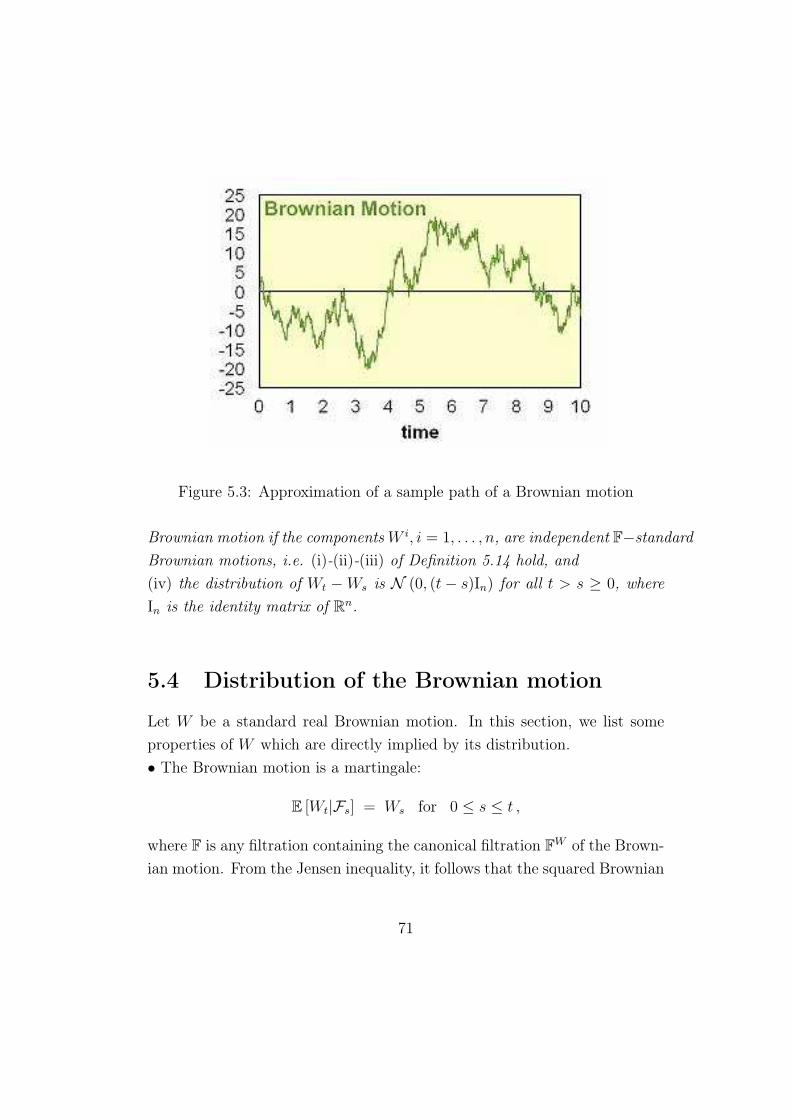
Figure 5.3: Approximation of a sample path of a Brownian motion
Brownian motion if the components W i, i = 1, . . . , n, are independent F−standard
Brownian motions, i.e. (i)-(ii)-(iii) of Definition 5.14 hold, and
(iv) the distribution of Wt −Ws is N (0, (t− s)In) for all t > s ≥ 0, where
In is the identity matrix of Rn.
5.4 Distribution of the Brownian motion
Let W be a standard real Brownian motion. In this section, we list some
properties of W which are directly implied by its distribution.
• The Brownian motion is a martingale:
E [Wt|Fs] = Ws for 0 ≤ s ≤ t ,
where F is any filtration containing the canonical filtration FW of the Brown-
ian motion. From the Jensen inequality, it follows that the squared Brownian
71

Figure 5.4: A sample path of the two-dimensional Brownian motion
motion W 2 is a submartingale:
E[
W 2t |Fs
]
≥ W 2s , for 0 ≤ s < t .
The precise departure from a martingale can be explicitly calculated
E[
W 2t |Fs
]
= W 2s + (t− s) , for 0 ≤ s < t ,
which means that the process W 2t − t, t ≥ 0 is a martingale.
• The Brownian motion is a Markov process, i.e.
E [φ (Ws, s ≥ t) |Ft] = E [φ (Ws, s ≥ t) |Wt]
for every t ≥ 0 and every bounded continuous function φ : C0(R+) −→ R,
where C0(R+) is the set of continuous functions from R+ to R. This follows
immediately from the fact thatWs−Wt is independent of Ft for every s ≥ t, a
72

consequence of the independence of the increments of the Brownian motion.
We shall see later in Corollary 5.2 that the Markov property holds in a
stronger sense by replacing the deterministic time t by an arbitrary stopping
time τ .
• The Brownian motion is a centered Gaussian process as it follows from
its definition that the vector random variable (Wt1 , . . . ,Wtn) is Gaussian for
every 0 ≤ t1 < . . . < tn. Centered Gaussian processes can be character-
ized in terms of their covariance function. A direct calculation provides the
covariance function of the Brownian motion
Cov (Wt,Ws) = E [WtWs] = t ∧ s = mint, s
The Kolmogorov theorem provides an alternative construction of the Brow-
nian motion as a centered Gaussian process with the above covariance func-
tion, we will not elaborate more on this and we send the interested reader to
Karatzas and Shreve [16], Section 2.2.
We conclude this section by the following property which is very useful
for the purpose of simulating the Brownian motion.
Exercise 5.9 For 0 ≤ t1 < t < t2, show that the conditional distribution
of Wt given (Wt1 ,Wt2) = (x1, x2) is Gaussian, and provided its mean and
variance in closed form. ♦
• By definition of the Brownian motion, for 0 ≤ t < T , the conditional
distribution of the random variable WT given Wt = x is a N (x, t− s):
p(t, x, T, y)dy := P [WT ∈ [y, y + dy]|Wt = x] =1
√
2π(T − t)e−
(y−x)2
2(T−t) dy
An important observation is that this density function satisfies the heat equa-
tion for every fixed (t, x):
∂p
∂T=
1
2
∂2p
∂y2,
73

as it can be checked by direct calculation. One can also fix (T, y) and express
the heat equation in terms of the variables (t, x):
∂p
∂t+
1
2
∂2p
∂x2= 0 . (5.2)
We next consider a function g with polynomial growth, say, and we define
the conditional expectation:
V (t, x) = E [g (WT ) |Wt = x] =
∫
g(y)p(t, x, T, y)dy . (5.3)
Since p is C∞, it follows from the dominated convergence theorem that V is
also C∞. By direct differentiation inside the integral sign, it follows that the
function V is a solution of
∂V
∂t+
1
2
∂2V
∂x2= 0 and V (T, .) = g . (5.4)
We shall see later in Section 6.3 that the function V defined in (5.3) is the
unique solution of the above linear partial differential equation in the class
of polynomially growing functions.
5.5 Scaling, symmetry, time reversal and trans-
lation
The following easy properties follow from the properties of the centered Gaus-
sian distribution.
Proposition 5.6 Let W be a standard Brownian motion, t0 > 0, and c > 0.
Then, so are the processes
• −Wt, t ≥ 0 (symmetry),
• √cWct, t ≥ 0 (scaling),
• Wt0+t −Wt0 , t ≥ 0 (time translation),
• WT−t −WT , 0 ≤ t ≤ T (time reversal).
74

Proof. Properties (i), (ii) and (iii) of Definition 5.15 are immediately
checked. ♦
Remark 5.7 For a Brownian motion W in Rn, the symmetry property of
the Brownian motion extends as follows: for any (n × n) matrix A, with
AAT = In, the process AWt, t ≥ 0 is a Brownian motion.
Another invariance property for the Brownian motion will be obtained
by time inversion in subsection 5.7 below. Indeed, the process B defined by
B0 := 0 and Bt := tW1/t, t > 0, obviously satisfies properties (ii) and (iii);
property (i) will be obtained as a consequence of the law of large numbers.
We next investigate whether the translation property of the Brownian
motion can be extended to the case where the deterministic time t0 is replaced
by some random time. The following result states that this is indeed the case
when the random time is a stopping time.
Proposition 5.7 Let W be a Brownian motion, and consider some stopping
time τ . Then, the process B defined by
Bt := Wt+τ −Wτ , t ≥ 0 ,
is a Brownian motion independent of Fτ .
Proof. Clearly B0 = 0 and B has a.s. continuous sample paths. In the
rest of this proof, we show that, for 0 ≤ t1 < t2 < t3 < t4, s > 0, and
bounded continuous functions φ, ψ and f :
E [φ (Bt4 −Bt3)ψ (Bt2 − Bt1) f (Ws)1s≤τ ]
= E [φ (Wt4 −Wt3)]E [ψ (Wt2 −Wt1)]E [f (Ws)1s≤τ ] (5.5)
This would imply that B has independent increments with the required Gaus-
sian distribution.
Observe that we may restrict our attention to the case where τ has a finite
support s1, . . . , sn. Indeed, given that (5.5) holds for such stopping times,
75

one may approximate a general stopping time τ by the decreasing sequence
of stopping times τn := (⌊nτ⌋+ 1) /n, apply (5.5) for each n ≥ 1, and pass
to the limit by the monotone convergence theorem thus proving that (5.5)
holds for τ .
For a stopping time τ with finite support s1, . . . , sn, we have:
E[
φ (Bt4 −Bt3)ψ (Bt2 −Bt1) f (Ws)1s≤τ]
=n∑
i=1
E[
φ (Bt4 −Bt3)ψ (Bt2 −Bt1) f (Ws)1s≤τ1τ=si]
=n∑
i=1
E
[
φ(
Wti4−Wti3
)
ψ(
Wti2−Wti1
)
f (Ws)1τ=si≥s]
where we denoted tik := si + tk for i = 1, . . . , n and k = 1, . . . , 4. We next
condition upon Fsi for each term inside the sum, and recall that 1τ=si is
Fsi−measurable as τ is a stopping time. This provides
E[
φ (Bt4 −Bt3)ψ (Bt2 −Bt1) f (Ws)1s≤τ]
=n∑
i=1
E
E
[
φ(
Wti4−Wti3
)
ψ(
Wti2−Wti1
)∣
∣
∣Fsi
]
f (Ws)1τ=si≥s
=n∑
i=1
E
E [φ (Wt4 −Wt3)]E [ψ (Wt2 −Wt1)] f (Ws)1τ=si≥s
where the last equality follows from the independence of the increments of
the Brownian motion and the symmetry if the Gaussian distribution. Hence
E[
φ (Bt4 −Bt3)ψ (Bt2 −Bt1) f (Ws)1s≤τ]
= E [φ (Wt4 −Wt3)]E [ψ (Wt2 −Wt1)]n∑
i=1
E[
f (Ws)1τ=si≥s]
which is exactly (5.5). ♦
An immediate consequence of Proposition 5.7 is the strong Markov prop-
erty of the Brownian motion.
76

Corollary 5.2 The Brownian motion satisfies the strong Markov property:
E [φ (Ws+τ , s ≥ 0) |Fτ ] = E [φ (Ws+τ , s ≥ 0) |Wτ ]
for every stopping time τ , and every bounded function φ : C0(R+) −→ R.
Proof. Since Bs := Ws+τ −Wτ is independent of Fτ for every s ≥ 0, we
have
E [φ (Ws+τ , s ≥ 0) |Fτ ] = E [φ (Bs +Wτ , s ≥ 0) |Fτ ]
= E [φ (Bs +Wτ , s ≥ 0) |Wτ ] .
♦
We next use the symmetry property of Proposition 5.7 in order to pro-
vide explicitly the joint distribution of the Brownian motion W and the
corresponding running maximum process:
W ∗t := sup
0≤s≤tWs , t ≥ 0 .
The key-idea for this result is to make use of the Brownian motion started
at the first hitting time of some level y:
Ty := inf t > 0 : Wt > y .
Observe that
W ∗t ≥ y = Ty ≤ t ,
which implies in particular a connection between the distributions of the
running maximum W ∗ and the first hitting time Ty.
Proposition 5.8 Let W be a Brownian motion and W ∗ the corresponding
running maximum process. Then, for t > 0, the random variables W ∗t and
|Wt| have the same distribution, i.e.
P [W ∗t ≥ y] = P [|Wt| ≥ y] .
77

Furthermore, the joint distribution of the Brownian motion and the corre-
sponding running maximum is characterized by
P [Wt ≤ x , W ∗t ≥ y] = P [Wt ≥ 2y − x] for y > 0 and x ≤ y .
Proof. From Exercise 5.6 and Proposition 5.7, the first hitting time Ty of
the level y is a stopping time, and the process
Bt :=(
Wt+Ty−WTy
)
, t ≥ 0 ,
is a Brownian motion independent of FTy. Since Bt and −Bt have the same
distribution and WTy= y, we compute that
P [Wt ≤ x , W ∗t ≥ y] = P
[
y + Bt−Ty≤ x , Ty ≤ t
]
= P[
y − Bt−Ty≤ x , Ty ≤ t
]
= P [Wt ≥ 2y − x , W ∗t ≥ y] = P [Wt ≥ 2y − x] ,
where the last equality follows from the fact that W ∗t ≥ y ⊂ Wt ≥ 2y−x
as x ≥ y. As for the marginal distribution of the running maximum, we
decompose:
P [W ∗t ≥ y] = P [Wt < y , W ∗
t ≥ y] + P [Wt ≥ y , W ∗t ≥ y]
= P [Wt < y , W ∗t ≥ y] + P [Wt ≥ y]
= 2P [Wt ≥ y] = P [|Wt| ≥ y]
where the two last equalities follow from the first part of this proof together
with the symmetry of the Gaussian distribution. ♦
The following property is useful for the approximation of Lookback op-
tions prices by Monte Carlo simulations.
Exercise 5.10 For a Brownian motion W and t > 0, show that
P [W ∗t ≥ y|Wt = x] = exp
(
−2
ty(y − x)
)
for y ≥ x+ .
78

5.6 On the filtration of the Brownian motion
Because the Brownian motion has a.s. continuous sample paths, the corre-
sponding canonical filtration is left-continuous, i.e. ∪s<tFWs = FW
t . How-
ever, FW is not right-continuous. To see this, observe that the event set
W has a local maximum at t is in FWt+ := ∩s>tFW
s , but is not in FWt .
This difficulty can be overcome by slightly enlarging the canonical filtra-
tion by the collection of zero-measure sets. We define N := A ∈ Ω : P(A) =
0 and the filtration by FWt := σ(FW
t ∪ N ).
The resulting filtration FW is called the completed canonical filtration,
and W remains a Brownian motion with respect to FW , because the four
properties of the Definition 5.14 do not depend on the null sets of P. Impor-
tantly, FW can be shown to be continuous. We send the interested reader to
Karatzas and Shreve [16] for a rigorous treatment of this question. In the
rest of these notes, we always work with the completed filtration, and since
there is no ambiguity, we shall from now on omit the bar in FW , that is, FW
will denote the completed filtration.
The following result appears simple, but has far-reaching consequences
for the study of local behavior of Brownian paths.
Proposition 5.9 (Blumenthal Zero-One law) Let W be a Brownian mo-
tion and FW its completed canonical filtration. If A ∈ FB0 then either
P (A) = 0 or P (A) = 1.
5.7 Small/large time behavior of the Brownian
sample paths
The discrete-time approximation of the Brownian motion suggests that Wt
t
tends to zero at least along natural numbers, by the law of large numbers.
With a little effort, we obtain the following strong law of large numbers for
the Brownian motion.
79
Theorem 5.11 For a Brownian motion W , we have
Wt
t−→ 0 P− a.s. as t→ ∞ .
Proof. We first decompose
Wt
t=
Wt −W⌊t⌋t
+⌊t⌋t
W⌊t⌋⌊t⌋
By the law of large numbers, we have
W⌊t⌋⌊t⌋ =
1
⌊t⌋
⌊t⌋∑
i=1
(Wi −Wi−1) −→ 0 P− a.s.
We next estimate that∣
∣Wt −W⌊t⌋∣
∣
t≤ ⌊t⌋
t
∣
∣∆⌊t⌋∣
∣
⌊t⌋ , where ∆n := supn−1<t≤n
|Wt −Wn−1| , n ≥ 1 .
Clearly, ∆n, n ≥ 1 is a sequence of independent identically distributed
random variables. The distribution of ∆n is explicitly given by Proposition
5.8. In particular, by a direct application of the Chebychev inequality, it is
easily seen that∑
n≥1 P[∆n ≥ nε] =∑
n≥1 P[∆1 ≥ nε] < ∞. By the Borel
Cantelli Theorem, this implies that ∆n/n −→ 0 P−a.s.
Wt −W⌊t⌋⌊t⌋ −→ 0 P− a.s. as t→ ∞ ,
and the required result follows from the fact that t/⌊t⌋ −→ 1 as t→ ∞. ♦
As an immediate consequence of the law of large numbers for the Brow-
nian motion, we obtain the invariance property of the Brownian motion by
time inversion:
Proposition 5.10 Let W be a standard Brownian motion. Then the process
B0 = 0 and Bt := tW 1t
for t > 0
is a Brownian motion.
80

Proof. All of the properties (i)-(ii)-(iii) of Definition 5.15 are obvious
except the sample path continuity at zero. But this is equivalent to the law
of large numbers stated in Proposition 5.11. ♦
The following two results show the complexity of the sample paths of the
Brownian motion.
Proposition 5.11 For any t0 ≥ 0, we have
lim inftցt0
Wt −Wt0
t− t0= −∞ and lim sup
tցt0
Wt −Wt0
t− t0= ∞ .
almost surely.
Proof. From the invariance of the Brownian motion by time transla-
tion, it is sufficient to consider t0 = 0. Observe that the random vari-
able lim suptց0Wt
tis in FB
0 , and therefore is deterministic. Assume that
lim suptց0Wt
t= C <∞. By symmetry of the Brownian motion, lim inftց0
Wt
t=
−C, and therefore lim Wt√t→ 0 p.s. However, by the scaling property Wt√
t∼
N(0, 1), which provides a contradiction. ♦
Proposition 5.12 Let W be a Brownian motion in R. Then, P−a.s. W
changes sign infinitely many times in any time interval [0, t], t > 0.
Observe that the event “W changes sign infinitely many times in any time
interval [0, t]” is in FB0 , and therefore its probability is either zero or one.
Assume that it is zero. Then, with probability one, either lim inftց0Wt
t= 0
or lim suptց0Wt
t= 0, which is a contradiction with Proposition 5.11.
♦
The following result shows that the sample paths of the Brownian motion
are unbounded a.s., and the Brownian motion is recurrent, meaning that this
process returns to the point 0 an infinite number of times.
81

Proposition 5.13 For a standard Brownian motion W , we have
lim supt→∞
Wt = ∞ and lim inft→∞
Wt = −∞
almost surely.
Proof.
From Proposition 5.10, Bt := tW1/t defines a Brownian motion. Since
Wt/t = B1/t, it follows that the behavior of Wt/t for t ց 0 corresponds to
the behavior of Bu for uր ∞. The required limit result is then a restatement
of Proposition 5.11 for t0 = 0. ♦
We conclude this section by stating, without proof, the law of the iterated
logarithm for the Brownian motion. The interested reader may consult [16]
for the proof.
Theorem 5.12 For a Brownian motion W , we have
lim supt→0
Wt√
2t ln(ln 1t)
= 1 and lim inft→0
Wt√
2t ln(ln 1t)
= −1
5.8 Quadratic variation
The purpose of this section is to study the variation of the Brownian motion
along dyadic sequences:
tni := i2−n , for integers i ≥ 0 and n ≥ 1 .
As we shall see shortly, the Brownian motion has infinite total variation.
In particular, this implies that classical integration theories are not suitable
for the case of the Brownian motion. The key-idea in order to define an
integration theory with respect to the Brownian motion is that the quadratic
variation is finite. In the context of these notes, we shall not present the
82

complete stochastic integration theory. We will restrict our attention to the
quadratic variation along dyadic sequences defined by
V nt :=
∑
tni ≤t
∣
∣
∣Wtni+1−Wtni
∣
∣
∣
2
for t > 0 .
More generally, given a continuous adapted stochastic process ϕ = ϕt, t ≥0, we define:
V nt (ϕ) :=
∑
tni ≤t
ϕtni
∣
∣
∣Wtni+1
−Wtni
∣
∣
∣
2
for t > 0 .
Before stating the main result of this section, we observe that the quadratic
variation (along any subdivision) of a continuously differentiable function f
converges to zero. Indeed,∑
ti≤t |f(ti+1)− f(ti)|2 ≤ ‖f ′‖L∞([0,t])
∑
ti≤t |ti+1−ti|2 −→ 0. Because of the non-differentiability property stated in Proposition
5.11, this result does not hold for the Brownian motion:
Proposition 5.14 Let W be a standard Brownian motion in R, and ϕ a
continuous adapted stochastic process with∫
R+|ϕt|2dt <∞ a.s. Then:
P
[
limn→∞
V nt (ϕ) =
∫ t
0
ϕsds , for every t ≥ 0
]
= 1 .
Proof. (i) We first assume that E
[
∫
R+|ϕt|2dt
]
< ∞, a condition which
will be relaxed in Step (iii) below. We first fix t > 0 and show that V nt (ϕ) −→
∫ t
0ϕsds P−a.s. as n→ ∞, or equivalently:
∑
tni ≤t
Zin→∞−→ 0 P− a.s. where Zi := ϕtni
(
(
Wtni+1−Wtni
)2
− 2−n
)
.
Observe that E[ZiZj] = 0 for i 6= j, and E[Z2j ] = C2−2nE
[
|ϕtni|2]
for some
constant C > 0. Then
∑
n≤N
E
∑
tni ≤t
Zi
2
=∑
n≤N
∑
tni ≤t
E[
Z2i
]
= C∑
n≤N
2−n∑
tni ≤t
E[
|ϕtni|2]
2−n .
83

Since∑
tni ≤t E[
|ϕtni|2]
2−n −→∫ t
0E [|ϕt|2] dt, we conclude that
lim infN→∞
E
∑
n≤N
∑
tni ≤t
Zi
2
< ∞ .
By Fatou’s lemma, this implies that
E
∑
n≥1
∑
tni ≤t
Zi
2
≤ lim infN→∞
∑
n≤N
E
∑
tni ≤t
Zi
2
< ∞ .
In particular, this shows that the series∑
n≥1
(
∑
tni ≤t Zi
)2
is a.s. finite, and
therefore∑
tni ≤t Zi −→ 0 P−a.s. as n→ ∞.
(ii) From the first step of this proof, we can find a zero measure set Ns
for each rational number s ∈ Q. For an arbitrary t ≥ 0, let (sp) and (s′p)
be two monotonic sequences of rational numbers with sp ր t and s′p ց t.
Then, except on the zero-measure set N := ∪s∈QNs, it follows from the
monotonicity of the quadratic variation that∫ sp
0
ϕudu = limn→∞
V nsp(ϕ) ≤ lim inf
n→∞V nt (ϕ)
≤ lim supn→∞
V nt (ϕ) ≤ lim
n→∞V ns′p(ϕ) =
∫ s′p
0
ϕudu .
Sending p→ ∞ shows that V nt (ϕ) −→
∫ t
0ϕudu as n→ ∞ for every ω outside
the zero-measure set N .
(iii) We now consider the general case where ϕ is only known to satisfy∫
R+|ϕt|2dt <∞ a.s. We introduce the sequence of stopping times
Tk := inf
t > 0 :
∫ t
0
|ϕu|2du ≥ k
, k ≥ 1 ,
and we observe that Tk −→ ∞ P−a.s. as k → ∞. From the previous steps
of this proof, we have P−a.s.∑
tni ≤t∧Tk
ϕtni
∣
∣
∣Wtni+1
−Wtni
∣
∣
∣
2
= V nt
(
ϕ1[0,Tk]
)
−→∫ t
0
ϕu1[0,Tk](u)du =
∫ t∧Tk
0
ϕudu .
84

The required limit result follows immediately by sending k → ∞. ♦
Remark 5.8 Proposition 5.14 has a natural direct extension to the multi-
dimensional setting. Let W be a standard Brownian motion in Rd, and let
ϕ be an adapted process with (d× d)−matrix values. Then, P−a.s.
∑
tni ≤t
Tr
[
ϕtni
(
Wtni+1−Wtni
)(
Wtni+1−Wtni
)T]
−→∫ t
0
Tr [ϕt] dt , t ≥ 0 .
We leave the verification of this result as an exercise.
Remark 5.9 Inspecting the proof of Proposition 5.14, we see that the
quadratic variation along any subdivision 0 = sn0 < . . . < snn = t satisfies:
n∑
i=1
∣
∣
∣Wsni+1−Wsni
∣
∣
∣
2
−→ t P− a.s. whenever∑
n≥1
sup1≤i≤n
|sni+1 − sni | −→ 0 .
We also observe that the above convergence result holds in probability for
an arbitrary partition (sni , 1 ≤ i ≤ n)n of [0, t] with mesh sup1≤i≤n |sni+1 − sni |shrinking to zero. See e.g. Karatzas and Shreve [16], Theorem 1.5.8 for the
case ϕ ≡ 1.
Proposition 5.14 implies, in particular, that the total variation of the
Brownian motion is not finite. This follows from the inequality
V nt ≤ max
tni ≤t
∣
∣
∣Wtni+1
−Wtni
∣
∣
∣
∑
i∈N
∣
∣
∣Wtni+1
−Wtni
∣
∣
∣1tni ≤t , (5.6)
together with the continuity of the Brownian motion which implies that
maxtni ≤t
∣
∣
∣Wtni+1−Wtni
∣
∣
∣ −→ 0. For this reason, the Stieltjes theory of inte-
gration does not apply to the Brownian motion.
85

Chapter 6
Integration to stochastic calculus
6.1 Stochastic integration with respect to the
Brownian motion
Recall from (5.6) that the total variation of the Brownian motion is infinite:
limn→∞
∑
tni ≤t
∣
∣
∣Wtni+1−Wtni
∣
∣
∣ = ∞ P− a.s.
Because of this property of the Brownian, one can not hope to define the
stochastic integral with respect to the Brownian motion pathwise. To un-
derstand this, let us forget for a moment about stochastic process. Let
ϕ, f : [0, 1] −→ R be continuous functions, and consider the Riemann sum:
Sn :=∑
tni ≤1
ϕ(
tni−1
) [
f (tni )− f(
tni−1
)]
.
The, if the total variation of f is infinite, one can not guarantee that the
above sum converges for every continuous function ϕ.
In order to circumvent this limitation, we shall make use of the finiteness
of the quadratic variation of the Brownian motion, which allows to obtain
an L2−definition of stochastic integration.
86

6.1.1 Stochastic integrals of simple processes
Throughout this section, we fix a final time T > 0. A process φ is called
simple if there exists a strictly increasing sequence (tn)n≥0 in R and a sequence
of random variables (ϕn)n≥0 such that
φt = ϕ010(t) +∞∑
n=0
ϕn1(tn,tn+1](t), t ≥ 0,
and
ϕn is Ftn − measurable for every n ≥ 0 and supn≥0
‖ϕn‖∞ <∞.
We shall denote by S the collection of all simple processes. For φ ∈ S, we
define its stochastic integral with respect to the Brownian motion by:
I0t (φ) :=∑
n≥0
ϕn
(
Wt∧tn+1 −Wt∧tn)
, 0 ≤ t ≤ T. (6.1)
By this definition, we immediately see that:
E[
I0t (φ)|Fs
]
= Is(φ) for 0 ≤ s ≤ t, (6.2)
i.e. I0t (X), t ≥ 0 is a martingale. We also calculate that
E[
I0t (φ)2]
= E
[∫ t
0
|φs|2ds]
for t ≥ 0. (6.3)
Exercise 6.11 Prove properties (6.2) and (6.3).
Our objective is to extend I0 to a stochastic integral operator I acting
on the larger set
H2 :=
φ : measurable, F− adapted processes with E
[∫ T
0
|φt|2dt]
<∞
,
which is a Hilbert space when equipped with the norm
‖φ‖H2 :=
(
E
[∫ T
0
|φt|2dt])1/2
.
This is crucially based on the following density result.
87

Proposition 6.15 The set of simple processes S is dense in H2, i.e. for
every φ ∈ H2, there is a sequence(
φ(n))
n≥0of processes in S such that
‖φ− φ(n)‖H2 −→ 0 as n→ ∞.
The proof of this result is reported in the Complements section 6.5.
6.1.2 Stochastic integrals of processes in H2
We now consider a process φ ∈ H2, and we intend to define the stochastic
integral It(φ) for every t ≥ 0 by using the density of simple processes.
a. From Proposition 6.15, there is a sequence(
φ(n))
n≥0which approximates
φ in the sense that ‖φ − φ(n)‖H2 −→ 0 as n → ∞. We next observe from
(6.3) that, for every t ≥ 0:
∥
∥I0t(
φ(n))
− I0t(
φ(m))∥
∥
2
L2 = E
[∫ t
0
|φ(n)s − φ(m)
s |2ds]
converges to zero as n,m→ ∞. This shows that the sequence(
I0t(
φ(n)))
n≥0
is a Cauchy sequence in L2, and therefore
I0t(
φ(n))
−→ It(φ) in L2 for some random variable It(φ).
b. We next show that the limit It(φ) does not depend on the choice of the
approximating sequence(
φ(n))
n. Indeed, for another approximating sequence
(
ψ(n))
nof φ, we have
∥
∥I0t(
ψ(n))
− It (φ)∥
∥
L2 ≤∥
∥I0t(
ψ(n))
− I0t(
φ(n))∥
∥
L2 +∥
∥I0t(
φ(n))
− It (φ)∥
∥
L2
≤∥
∥ψ(n) − φ(n)∥
∥
H2 +∥
∥I0t(
φ(n))
− It (φ)∥
∥
L2
−→ 0 as n→ ∞.
c. We finally show that the uniquely defined limit It(φ) satisfies the ana-
logue properties of (6.2)-(6.3):
E [It(φ)|Fs] = Is(φ) for 0 ≤ s ≤ t and φ ∈ H2, (6.4)
E[
It(φ)2]
= E
[∫ t
0
|φt|2dt]
for t ≥ 0 and φ ∈ H2. (6.5)
88

To see that (6.4) holds, we directly compute with(
φ(n))
nan approximating
sequence of φ in H2 that
‖E [It(φ)|Fs]− Is(φ)‖L2 ≤∥
∥E [It(φ)|Fs]− E[
I0t (φ(n))|Fs
]∥
∥
L2
+∥
∥E[
I0t (φ(n))|Fs
]
− Is(φ)∥
∥
L2
=∥
∥E [It(φ)|Fs]− E[
I0t (φ(n))|Fs
]∥
∥
L2
+∥
∥I0s (φ(n))− Is(φ)
∥
∥
L2
by (6.2). By the Jensen inequality and the law of iterated expectations, this
provides
‖E [It(φ)|Fs]− Is(φ)‖L2 ≤∥
∥It(φ)− I0t (φ(n))∥
∥
L2 +∥
∥I0s (φ(n))− Is(φ)
∥
∥
L2
which implies (6.4) by sending n to infinity.
As for (6.5), it follows from the H2− convergence of φ(n) towards φ and
the L2−convergence of I0(
φ(n))
towards I(φ), together with (6.3), that:
E
[∫ t
0
|φs|2ds]
= limn→∞
E
[∫ t
0
|φ(n)s |2ds
]
= limn→∞
E
[
I0(
φ(n))2]
= E[
I (φ)2]
.
Summarizing the above construction, we have proved the following.
Theorem 6.13 For φ ∈ H2 and t ≥ 0, the stochastic integral denoted
It(φ) :=
∫ t
0
φsdWs
is the unique limit in L2 of the sequence(
I0t (φ(n)))
nfor every choice of an
approximating sequence(
φ(n))
nof φ in H2. Moreover, It(φ), t ≥ 0 is a
square integrable martingale satisfying the Itô isometry
E
[
(∫ t
0
φsdWs
)2]
= E
[∫ t
0
|φs|2ds]
, t ≥ 0.
Observe that, since the Brownian motion has continuous trajectories, the
stochastic integral of a simple process I0(φ) also has continuous sample paths
89

by the definition in (6.1). It is not clear whether this property is inherited
by the extension I of I0 to H2. The following result shows that it is indeed
the case, and provides the useful Doob’s maximal inequality for martingales
(6.6).
Proposition 6.16 Let φ be a process in H2, and set Mt :=∫ t
0φs ·dWs, t ≥ 0.
Then M has continuous sample paths a.s. and
E
[
sups≤t
Ms
]
≤ 4E[
|Ms|2]
= E
[∫ t
0
|φs|2ds]
. (6.6)
Proof. 1. Set M∗t := sups≤tMs. In this step, we prove that the maximal
inequality (6.6) holds if M is known to to be continuous. Consider the
sequence of stopping times:
θn := inf t ≥ 0 : M∗t ≥ n
Observing that X∗ is a non-decreasing process and Mt =M∗t on dM∗
t > 0,it follows that
d(M∗t )
2 = 2M∗t dM
∗t = 2MtdM
∗t = 2 [d(MtM
∗t )−M∗
t dMt] .
Then
(
M∗t∧θn)2
= 2Mt∧θnM∗t∧θn − 2
∫ t∧θn
0
M∗s dMs
Since 0 ≤M∗ ≤ n on [0, θn], this implies that
E
[
(
M∗t∧θn)2]
= 2E[
Mt∧θnM∗t∧θn]
≤ 2E[
M2t∧θn]1/2
E
[
(
M∗t∧θn)2]1/2
by the Cauchy-Schwartz inequality. Hence
E
[
(
M∗t∧θn)2]
≤ 4E[
M2t∧θn]
= E
[∫ t∧θn
0
|φs|2ds]
≤ E
[∫ t
0
|φs|2ds]
and we obtain the maximal inequality by sending n to infinity and using the
monotone convergence theorem.
90

2. We now show that the process M is continuous. By definition of the
stochastic integral, Mt is the L2−limit of Mnt := I0t (φ
n) for some sequence
(φn)n of simple processes converging to φ in H2. By definition of the stochas-
tic integral of simple integrands in (6.1), notice that the process Mnt −Mm
t =
I0t (φn) − I0t (φ
m), t ≥ 0 is a.s. continuous. We then deduce from the first
step that:
E
[
sups≤t
|Mns −Mm
s |]
≤ E
[
sups≤t
(Mns −Mm
s )
]
+ E
[
sups≤t
(Mms −Mn
s )
]
≤ 8 E
[∫ t
0
|φns − φm
s |2ds]
.
This shows that the sequence (Mn)n is a Cauchy sequence in the Banach
space of continuous processes endowed with the norm E[
sup[0,T ] |Xs|]
. Then
Mn converges towards a continuous process M in the sense of this norm. We
know however that Mn −→ M := I.(φ) in H2. By passing to subequences
we may deduce that M =M is continuous.
3. From the previous step, we know that M is continuous. We are then in
the context of step 1, and we may deduce that the maximal inequality (6.6)
holds for M . ♦
Exercise 6.12 Let f : [0, T ] −→ Rd be a deterministic function with∫ T
0|f(t)|2dt <
∞. Prove that∫ T
0
f(t) · dWt has distribution N(
0,
∫ T
0
|f(t)|2dt)
.
Hint: Use the closeness of the Gaussian space.
6.1.3 Stochastic integration beyond H2
Our next task is to extend the stochastic integration to integrands φ such
that
φ is F− adapted and
∫ T
0
|φt|2dt <∞ P− a.s. for every T > 0. (6.7)
91

To do this, we consider the sequence of stopping times
τn := inf
t > 0 :
∫ t
0
|φu|2du ≥ n
.
Clearly, (τn)n is a non-decreasing sequence of stopping times and
τn −→ ∞ P− a.s. when n→ ∞.
For fixed n > 0, the stopped process φnt := φt1t≤τn is in H2. Then the
stochastic integral It (φn) is well-defined by Theorem 6.13. Since (τn)n is a
non-decreasing and P [τn ≥ t for some n ≥ 1] = 1, it follows that the limit
It(φ) := (a.s.) limn→∞
It (φn) (6.8)
exists (in fact It (φ) = It (φn) for n sufficiently large, a.s.).
Remark 6.10 The above extension of the stochastic integral to integrands
satisfying (6.7) does not imply that It(φ) satisfies properties (6.4) and (6.5).
This issue will be further developed in the next subsection. The maximal
inequality (6.6) is also lost since the stochastic integral is not known to be in
L2. However the continuity property of the stochastic integral is conserved
because it is a pathwise property which is consistent with the pathwise defi-
nition of (6.8).
As a consequence of this remark, when the integrand φ satisfies (6.7) but
is not in H2, the stochastic integral fails to be a martingale, in general. This
leads us to the notion of local martingale.
Definition 6.17 An F−adapted process M = Mt, t ≥ 0 is a local mar-
tingale if there exists a sequence of stopping times (τn)n≥0 (called a localizing
sequence) such that τn −→ ∞ P−a.s. as n → ∞, and the stopped process
M τn = Mt∧τn , t ≥ 0 is a martingale for every n ≥ 0.
Proposition 6.17 Let φ be a process satisfying (6.7). Then, for every T >
0, the process It(φ), 0 ≤ t ≤ T is a local martingale.
92

Proof. The above defined sequence (τn)n is easily shown to be a localizing
sequence. The result is then a direct consequence of the martingale property
of the stochastic integral of a process in H2. ♦
An example of local martingale which fails to be a martingale will be
given in the next subsection.
6.2 Itô’s formula
The purpose of this section is to prove the Itô formula for the change of
variable. Given a smooth function f(t, x), we will denote by ft, fx and fxx,
the partial gradients with respect to t, to x, and the partial Hessian matrix
with respect to x.
Theorem 6.14 Let f : R+ × Rd −→ R be C1,2(
[0, T ],Rd)
. Then, with
probability 1, we have:
f(T,WT ) = f(0, 0) +
∫ T
0
fx (t,Wt) · dWt +
∫ T
0
(
ft +1
2Tr[fxx]
)
(t,Wt)dt
for every T ≥ 0.
Proof. 1 We first fix T > 0, and we show that the above Itô’s formula
holds with probability 1. By possibly adding a constant to f we may assume
that f(0, 0) = 0. Let tni := i2−n for i ≥ 1, and n(T ) := ⌊T2n⌋, so that
tnn(T ) ≤ T < tnn(T )+1.
1.a We first decompose
f(
tnn(T )+1,Wtnn(T )+1
)
=∑
tni ≤T
[
f(
tni+1,Wtni+1
)
− f(
tni ,Wtni+1
)]
+∑
tni ≤T
[
f(
tni ,Wtni+1
)
− f(
tni ,Wtni
)
]
.
93

By a Taylor expansion, this provides:
InT (fx) :=∑
tni ≤T
fx(
tni ,Wtni
)
·(
Wtni+1−Wtni
)
= f(
tnn(T )+1,Wtnn(T )+1
)
−∑
tni ≤T
ft
(
τni ,Wtni+1
)
2−n
−1
2
∑
tni ≤T
Tr[(
fxx (tni , ξ
ni )− fxx
(
tni ,Wtni
))
∆niW∆n
iWT]
−1
2
∑
tni ≤T
Tr[
fxx(
tni ,Wtni
)
∆niW∆n
iWT]
, (6.9)
where ∆niW := Wtni+1
−Wtni, τni is a random variable with values in
[
tni , tni+1
]
,
and ξni = λniWtni+(1− λni )Wtni+1
for some random variable λni with values in
[0, 1].
1.b Since a.e. sample path of the Brownian motion is continuous, and
therefore uniformly continuous on the compact interval [0, T + 1], it follows
that
f(
tnn(T )+1,Wtnn(T )+1
)
−→ f(T,WT ) , P− a.s.
∑
tni ≤T ft
(
τni ,Wtni+1
)
2−n −→∫ T
0ft(t,Wt)dt P− a.s.
and with Proposition 5.14:∑
tni ≤T
Tr[(
fxx (tni , ξ
ni )− fxx
(
tni ,Wtni
))
∆niW∆n
iWT]
−→ 0 P− a.s.
Finally, from Proposition 5.14 and its multi-dimensional extension in Remark
5.8, the last term in the decomposition (6.9):
∑
tni ≤T
Tr[
fxx(
tni ,Wtni
)
∆niW∆n
iWT]
−→∫ T
0
Tr [fxx (t,Wt)] dt P− a.s. .
1.c In order to complete the proof of Itô’s formula for fixed T > 0, it
remains to prove that
InT (fx) −→∫ T
0
fx(t,Wt) · dWt P− a.s. along some subsequence.(6.10)
94

Notice that InT (fx) = I0T(
φ(n))
where φ(n) is the simple process defined by
φ(n)t =
∑
tni ≤T
fx(
tni ,Wtni
)
1[tni ,tni+1)(t), t ≥ 0.
Since φ(n) −→ φ in H2 with φt := fx (t,Wt), it follows from the definition
of the stochastic integral in Theorem 6.13 that InT (fx) −→ IT (φ) in L2,
and (6.10) follows from the fact that the L2 convergence implies the a.s.
convergence along some subsequence.
2. From the first step, we have the existence of subsets Nt ⊂ F for every
t ≥ 0 such that P[Nt] = 0 and the Itô’s formula holds on N ct , the complement
of Nt. Of course, this implies that the Itô’s formula holds on the complement
of the set N := ∪t≥0Nt. But this does not complete the proof of the theorem
as this set is a non-countable union of zero measure sets, and is therefore not
known to have zero measure. We therefore appeal to the continuity of the
Brownian motion and the stochastic integral, see Proposition 6.16. By usual
approximation along rational numbers, it is easy to see that, with probability
1, the Itô formula holds for every T ≥ 0. ♦
Remark 6.11 Since, with probability 1, the Itô formula holds for every
T ≥ 0, it follows that the Itô’s formula holds when the deterministic time T
is replaced by a random time τ .
6.2.1 Extension to Itô processes
We next provide Itô’s formula for a general Itô process, that is an Rn-valued
process defined by:
Xt := X0 +
∫ t
0
µsds+
∫ t
0
σsdWs, t ≥ 0,
where µ and σ are adapted processes with values in Rn and MR(n, d), re-
spectively and satisfying
∫ T
0
|µs|ds+∫ T
0
|σs|2ds <∞ a.s.
95
Observe that stochastic integration with respect to the Itô process X re-
duces to the stochastic integration with respect to W : for any F−adapted
Rn−valued process φ with∫ T
0|σT
t φt|2dt+∫ T
0|φt · µt|dt <∞,a.s.
∫ T
0
φt · dXt =
∫ T
0
φt · µtdt+
∫ T
0
φt · σtdWt
=
∫ T
0
φt · µtdt+
∫ T
0
σTt φt · dWt.
Theorem 6.15 Let f : R+ × Rn −→ R be C1,2 ([0, T ],Rn). Then, with
probability 1, we have:
f(T,XT ) = f(0, 0) +
∫ T
0
fx (t,Xt) · dXt
+
∫ T
0
(
ft(t,Xt) +1
2Tr[fxx(t,Xt)σtσ
Tt ]
)
dt
for every T ≥ 0.
Proof. Let θN := inf
t : max(
|Xt −X0|,∫ t
0σ2sds,
∫ t
0|µs|ds
)
≥ N
. Obvi-
ously, θN → ∞ a.s. when N → ∞, and it is sufficient to prove Itô’s formula
on [0, θN ], since any t ≥ 0 can be reached by sending N to infinity. In view
of this, we may assume without loss of generality that X,∫ t
0µsds,
∫ t
0σ2sds
are bounded and that f has compact support. We next consider an approx-
imation of the integrals defining Xt by step functions which are constant on
intervals of time [tni−1, tni ) for i = 1, . . . , n, and we denote by Xn the resulting
simple approximating process. Notice that Itô’s formula holds true for Xn
on each interval [ti−1, ti) as a direct consequence of Theorem 6.14. The proof
of the theorem is then concluded by sending n to infinity, and using as much
as needed the dominated convergence theorem. ♦
Exercise 6.13 Let W be a Brownian motion and consider the process
Xt := X0 + bt+ σWt , t ≥ 0 ,
96

where b is a vector in Rd and σ is an (d×d)−matrix. Let f be a C1,2(R+,Rd)
function. Show that
df(t,Xt) =∂f
∂t(t,Xt)dt+
∂f
∂x(t,Xt) · dXt +
1
2Tr
[
∂2f
∂x∂xT(t,Xt)σσ
T
]
.
We conclude this section by providing an example of local martingale
which fails to be a martingale, although positive and uniformly integrable.
This shows the limitation of the discrete-time result of Lemma 3.1.
Example 6.14 Let W be a Brownian motion in Rd.
• In the one-dimensional case d = 1, we have P [|Wt| > 0, ∀ t > 0] = 0, see
also Proposition 5.12.
• When d ≥ 2, the situation is drastically different as it can be proved
that P [|Wt| > 0, for every t > 0] = 1, see e.g. Karatzas and Shreve [16]
Proposition 3.22 p161. In words, this means that the Brownian motion never
returns to the origin P−a.s. Then, for a fixed t0 > 0, the process
Xt := |Wt0+t|−1 , t ≥ 0 ,
is well-defined, and it follows from Itô’s formula that
dXt = X3t
(
1
2(3− d)dt−Wt · dWt
)
.
• We now consider the special case d = 3. By the previous Proposition
6.17, it follows from Itô’s formula that X is a local martingale. However, by
the scaling property of the Brownian motion, we have
E[Xt] =
√
t0t+ t0
E[X0] , t ≥ 0 ,
so that X has a non-constant expectation and can not be a martingale.
• Passing to the polar coordinates, we calculate directly that
E[
X2t
]
= (2π(t0 + t))−3/2
∫
|x|−2e−|x|2/2(t0+t)dx
= (2π(t0 + t))−3/2
∫
r−2e−r2/2(t0+t)4πr2dr
=1
t0 + t≤ 1
t0for every t ≥ 0.
97

This shows that supt≥0 E [X2t ] <∞. In particular, X is uniformly integrable.
6.3 The Feynman-Kac representation formula
In this section, we consider the following linear partial differential equation
∂v
∂t+ b · ∂v
∂x+
1
2Tr
[
∂2v
∂x∂xTσσT
]
− kv + f = 0 , t < T, x ∈ Rd(6.11)
v(T, .) = g (6.12)
where g is a given function from Rd to R, k and f are functions from [0, T ]×Rd
to R, b is a constant vector in Rd, and σ is a constant d × d matrix. This
is the so-called Dirichlet problem. The following result provides a stochastic
representation for the solution of this purely deterministic problem.
Theorem 6.16 Assume that the function k is uniformly bounded from below,
and f has polynomial growth in x uniformly in t. Let v be a C1,2(
[0, T ),Rd)
solution of (6.11) with polynomial growth in x uniformly in t. Then
v(t, x) = E
[∫ T
t
βt,xs f(s,X t,x
s )ds+ βt,xT g
(
X t,xT
)
]
, t ≤ T, x ∈ Rd ,
where X t,xs := x + b(s − t) + σ(Ws − Wt) and βt,x
s := e−∫ stk(u,Xt,x
u )du for
t ≤ s ≤ T .
Proof. We first introduce the sequence of stopping times
τn := T ∧ inf
s > t :∣
∣X t,xs − x
∣
∣ ≥ n
,
and we oberve that τn −→ T P−a.s. Since v is smooth, it follows from Itô’s
formula that for t ≤ s < T :
d(
βt,xs v
(
s,X t,xs
))
= βt,xs
(
−kv + ∂v
∂t+ b · ∂v
∂x+
1
2Tr
[
∂2v
∂x∂xTσσT
])
(
s,X t,xs
)
ds
+βt,xs
∂v
∂x
(
s,X t,xs
)
σdWs
= βt,xs
(
−f(s,X t,xs )ds+
∂v
∂x
(
s,X t,xs
)
σdWs
)
,
98

by the PDE satisfied by v in (6.11). Then:
E[
βt,xτn v
(
τn, Xt,xτn
)]
− v(t, x)
= E
[∫ τn
t
βt,xs
(
−f(s,Xs)ds+∂v
∂x
(
s,X t,xs
)
σdWs
)]
.
Now observe that the integrands in the stochastic integral is bounded by def-
inition of the stopping time τn and the smoothness of v. Then the stochastic
integral has zero mean, and we deduce that
v(t, x) = E
[∫ τn
t
βt,xs f
(
s,X t,xs
)
ds+ βt,xτn v
(
τn, Xt,xτn
)
]
. (6.13)
Since τn −→ T and the Brownian motion has continuous sample paths P−a.s.
it follows from the continuity of v that, P−a.s.∫ τn
t
βt,xs f
(
s,X t,xs
)
ds+ βt,xτn v
(
τn, Xt,xτn
)
n→∞−→∫ T
t
βt,xs f
(
s,X t,xs
)
ds+ βt,xT v
(
T,X t,xT
)
=
∫ T
t
βt,xs f
(
s,X t,xs
)
ds+ βt,xT g
(
X t,xT
)
(6.14)
by the terminal condition satisfied by v in (6.11). Moreover, since k is
bounded from below and the functions f and v have polynomial growth
in x uniformly in t, we have∣
∣
∣
∣
∫ τn
t
βt,xs f
(
s,X t,xs
)
ds+ βt,xτn v
(
τn, Xt,xτn
)
∣
∣
∣
∣
≤ C
(
1 + supt≤T
|Wt|p)
.
By Proposition 5.8, the latter bound is integrable, and we deduce from
the dominated convergence theorem that the convergence in (6.14) holds
in L1(P), proving the required result by taking limits in (6.13). ♦
The above Feynman-Kac representation formula can be extended to the
case where the coefficients b and σ of the partial differential equation (6.11)
are functions of (t, x). In this case, the process X in the representation
formula is defined as the solution of a stochastic differential equation.
99

We also observe that the Feynman-Kac representation formula has an
important numerical implication. Indeed it opens the door to the use of
Monte Carlo methods in order to obtain a numerical approximation of the
solution of the partial differential equation (6.11). For sake of simplicity, we
provide the main idea in the case f = k = 0. Let(
X(1), . . . , X(k))
be an iid
sample drawn in the distribution of X t,xT , and compute the mean:
vk(t, x) :=1
k
k∑
i=1
g(
X(i))
.
By the Law of Large Numbers, it follows that vk(t, x) −→ v(t, x) P−a.s.
Moreover the error estimate is provided by the Central Limit Theorem:
√k (vk(t, x)− v(t, x))
k→∞−→ N(
0,Var[
g(
X t,xT
)])
in distribution,
and is remarkably independent of the dimension d of the variable X !
6.4 The Cameron-Martin change of measure
Let N be a Gaussian random variable with mean zero and unit variance. The
corresponding probability density function is
∂
∂xP[N ≤ x] = f(x) =
1√2π
e−x2/2 , x ∈ R .
For any constant a ∈ R, the random variable N + a is Gaussian with mean
a and unit variance with probability density function
∂
∂xP[N + a ≤ x] = f(x− a) = f(x)eax−
a2
2 , x ∈ R .
Then, for every (at least bounded) function ψ, we have
E [ψ(N + a)] =
∫
ψ(x)f(x)eax−a2
2 dx = E
[
eaN−a2
2 ψ(N)]
.
This easy result can be translated in terms of a change of measure. Indeed,
since the random variable eaN−a2
2 is positive and integrates to 1, we may
100

introduce the equivalent measure Q := eaN−a2
2 · P. Then, the above equality
says that the Q−distribution ofN coincides with the P−distribution ofN+a,
i.e.
under Q, N − a is distributed as N (0, 1) .
The purpose of this section is to extend this result to a Brownian motion
W in Rd. Let h : [0, T ] −→ Rd be a deterministic function in L2, i.e.∫ T
0|h(t)|2dt <∞. From Theorem 6.13, the stochastic integral
N :=
∫ T
0
h(t) · dWt
is well-defined as the L2−limit of the stochastic integral of some H2−approximating
simple function. In particular, since the space of Gaussian random variables
is closed, it follows that
N is distributed as N(
0,
∫ T
0
|h(t)|2dt)
,
and we may define an equivalent probability measure Q by:
dQ
dP:= e
∫ T0 h(t)·dWt− 1
2
∫ T0 |h(t)|2dt . (6.15)
Theorem 6.17 For a Brownian motion W in Rd, let Q be the probability
measure equivalent to P defined by (6.15). Then, the process
Bt := Wt −∫ t
0
h(u)du , t ∈ [0, T ] ,
is a Brownian motion under Q.
Proof. We first observe that B0 = 0 and B has a.s. continuous sample
paths. It remains to prove that, for 0 ≤ s < t, Bt − Bs is independent of Fs
and distributed as a centered Gaussian with variance t − s. To do this, we
compute the Q−Laplace transform
EQ[
eλ·(Wt−Ws)∣
∣Fs
]
= E
[
e∫ tsh(u)·dWu− 1
2
∫ ts|h(u)|2dueλ·(Wt−Ws)
∣
∣
∣Fs
]
= e−12
∫ ts|h(u)|2duE
[
e∫ ts(h(u)+λ)·dWu
∣
∣
∣Fs
]
101

Since the random variable∫ t
s(h(u) + λ) · dWu is a centered Gaussian with
variance∫ t
s|h(u) + λ|2du, independent of Fs, this provides:
EQ[
eλ·(Wt−Ws)∣
∣Fs
]
= e−12
∫ ts|h(u)|2due
12
∫ ts|h(u)+λ|2du
= e12λ2(t−s)+λ
∫ tsh(u)du .
This shows thatWt−Ws is independent of Fs and is distributed as a Gaussian
with mean∫ t
sh(u)du and variance t − s, i.e. Bt − Bs is independent of Fs
and is distributed as a centered Gaussian with variance t− s. ♦
Let us observe that the above result can be extended to the case where
h is an adapted stochastic process satisfying some convenient integrability
conditions. This is the so-called Girsanov theorem. In the context of these
lectures, we shall only need the Gaussian framework of the Cameron-Martin
formula.
6.5 Complement: density of simple processes
in H2
The proof of Proposition 6.15 is a consequence of the following Lemmas.
Throughout this section, tni := i2−n, i ≥ 0 is the sequence of dyadic numbers.
Lemma 6.4 Let φ be a bounded F−adapted process with continuous sample
paths. Then φ can be approximated by a sequence of simple processes in H2.
Proof. Define the sequence
φ(n)t := φ010(t) +
∑
tni ≤T
φtni1(tni ,t
ni+1]
(t), t ≤ T.
Then, φ(n) is a simple process for each n ≥ 1. By the dominated convergence
theorem, E[
∫ T
0|φ(n)
t − φt|2]
−→ 0 as n→ ∞. ♦
102

Lemma 6.5 Let φ be a bounded F−progressively measurable process. Then
φ can be approximated by a sequence of simple processes in H2.
Proof. Notice that the process
Y(k)t := k
∫ t∧T
0∨(t−k−1)
Xsds, t ≥ 0,
is progressively measurable as the difference of two adapted continuous pro-
cesses, see Proposition 5.5, and satisfies
∥
∥Y (k) −X∥
∥
H2 −→ 0 as k → ∞, (6.16)
by the dominated convergence theorm. For each k ≥ 1, we can find by Lemma
6.4 a sequence(
Y (k,n))
n≥0of simple processes such that ‖Y (k,n)−Y (k)‖H2 −→
0 as n→ ∞. Then, for each k ≥ 0, we can find nk such that
the process X(k) := Y (k,nk) satisfies∥
∥X(k) −X∥
∥
H2 −→ 0 as k → ∞.
♦
Lemma 6.6 Let φ be a bounded measurable and F−adapted process. Then
φ can be approximated by a sequence of simple processes in H2.
Proof. In the present setting, the process Y (k), defined in the proof of the
previous Lemma 6.5, is measurable but is not known to be adapted. For each
ε > 0, there is an integer k ≥ 1 such that Y ε := Y (k) satisfies ‖Y ε−X‖H2 ≤ ε.
Then, with Xt = X0 for t ≤ 0:
‖X −X.−h‖H2 ≤ ‖X − Y ε‖H2 +∥
∥Y ε − Y ε.−h
∥
∥
H2 +∥
∥Y ε.−h −X.−h
∥
∥
H2
≤ 2ε+∥
∥Y ε − Y ε.−h
∥
∥
H2 .
By the continuity of Y ε, this implies that
lim suphց0
‖X −X.−h‖H2 ≤ 4ε2. (6.17)
103

We now introduce
ϕn(t) := 10(t) +∑
i≥1
tni 1(tni−1,tni ],
and
X(n,s)t := Xϕn(t−s)+s, t ≥ 0, s ∈ (0, 1].
Clearly Xn,s is a simple adapted process, and
E
[∫ T
0
∫ 1
0
|X(n,s)t −Xt|2dsdt
]
= 2nE
[
∫ T
0
∫ 2−n
0
|Xt −Xt−h|2dhdt]
= 2n∫ 2−n
0
E
[∫ T
0
|Xt −Xt−h|2dt]
dh
≤ max0≤h≤2−n
E
[∫ T
0
|Xt −Xt−h|2dt]
which converges to zero as n→ ∞ by (6.17). Hence
X(n,s)t (ω) −→ Xt(ω) for almost every (s, t, ω) ∈ [0, 1]× [0, T ]× Ω,
and the required result follows from the dominated convergence theorem.
♦
Lemma 6.7 The set of simple processes S is dense in H2.
Proof. We only have to extend Lemma 6.6 to the case where φ is not
necessarily bounded. This is easily achieved by applying Lemma 6.6 to the
bounded process φ ∧ n, for each n ≥ 1, and passing to the limit as n → ∞.
♦
104

Chapter 7
Financial markets in continuous
time
Let T be a finite horizon, and (Ω,F , P ) be a complete probability space
supporting a Brownian motion W = (W 1t , . . . ,W
dt ), 0 ≤ t ≤ T with values
in Rd. We denote by F = Ft, 0 ≤ t ≤ T the (continuous) canonical
completed filtration of W , i.e. the canonical filtration augmented by zero
measure sets. For simplicity, we shall always assume that F = FT .
The financial market consists in d+ 1 assets :
(i) The first asset S0 is non-risky, and is defined by
S0t = exp
(∫ t
0
r(u)du
)
, 0 ≤ t ≤ T ,
where r : [0, T ] −→ R+ is a deterministic instantaneous interest rate function
satisfying∫ T
0
r(t)dt < ∞.
(ii) The d remaining assets Si, i = 1, . . . , d, are risky assets with price
processes :
Sit = Si
0 exp
(
∫ t
0
(
bi(u)− 1
2
d∑
j=1
∣
∣σij(t)∣
∣
2
)
dt+d∑
j=1
∫ t
0
σij(t)dW jt
)
, t ≥ 0 ,
105

for 1 ≤ i ≤ d. Here b =(
b1, . . . , bd)
and σ = (σij) are determinstic functions
on [0, T ] with values respectively in Rd and MR(d, d), the set of d×d matrices
with real coefficients. In order for the above stochastic integral to be well-
defined, we assume that
∫ T
0
(
|b(t)|+ |σ(t)|2)
dt < ∞.
By a direct application of Itô’s formula, it follows that:
dSit = Si
t
(
bi(t)dt+d∑
j=1
σij(t)dW jt
)
,
or in vector notations:
dSt = diag[St] (b(t)dt+ σ(t)dWt) .
where, for z ∈ Rn, diag[z] denotes the diagonal matrix with diagonal elements
zi. We assume that the MR(d, d)−matrix σ(t) is invertible for every t ∈[0, T ], and we introduce the function
λ0(t) := σ(t)−1 (b(t)− r(t)) , 0 ≤ t ≤ T ,
called the risk premium. We shall frequently make use of the discounted
process
St :=St
S0t
= St exp
(
−∫ t
0
r(u)du
)
,
where S = (S1, . . . , Sd). Using the above matrix notations, the dynamics of
the process S are given by in
dSt = diag[St] (b(t)− r(t)1)dt+ σ(t)dWt = diag[St]σ(t)(
λ0(t)dt+ dWt
)
where 1 = (1, . . . , 1) ∈ Rd.
106

7.1 Portfolio and wealth process
A portfolio strategy is an F−adapted process π = πt, 0 ≤ t ≤ T with
values in Rd. For 1 ≤ i ≤ n and 0 ≤ t ≤ T , πit is the amount (in Euros)
invested in the risky asset Si.
As in the discrete-time financial market, we shall consider self-financing
strategies. LetXt denote the wealth process at time t induced by the portfolio
strategy π. Then, the amount invested in the non-risky asset is Xt−∑n
i=1 πit
= Xt − πt · 1.
Under the self-financing condition, the dynamics of the wealth process is
given by
dXt =n∑
i=1
πit
Sit
dSit +
Xt − πt · 1S0t
dS0t
Let X be the discounted wealth process
Xt := Xt exp
(
−∫ t
0
r(u)du
)
, 0 ≤ t ≤ T .
Then, by an immediate application of Itô’s formula, we see that
dXt = πt · diag[St]−1dSt (7.1)
= πt · σ(t)(
λ0(t)dt+ dWt
)
, 0 ≤ t ≤ T . (7.2)
We still have to place further technical conditions on π, at least for the above
wealth process to be well-defined as a stochastic integral. Before this, let us
observe that, assuming that the risk premium function satisfies:
∫ T
0
∣
∣λ0(t)∣
∣
2dt < ∞ ,
it follows from the Cameron-Martin change of measure theorem that the
process
W 0t := Wt −
∫ t
0
λ0(u)du , 0 ≤ t ≤ T , (7.3)
107

is a Brownian motion under the equivalent probability measure
P0 := Z0T · P on FT , (7.4)
where
Z0T := exp
(
−∫ T
0
λ0(u) · dWu −1
2
∫ T
0
|λ0(u)|2du)
. (7.5)
In terms of the P0 Brownian motion W 0, the discounted wealth process in-
duced by an initial capital x and a portfolio strategy π can be written in
Xx,πt = X0 +
∫ t
0
πu · σ(u)dW 0u , 0 ≤ t ≤ T . (7.6)
Definition 7.18 An admissible portfolio process π = πt, t ∈ [0, T ] is an
F−adapted process such that the stochastic integral (7.6) is well-defined, and
the corresponding discounted wealth process satisfies the finite credit line con-
dition
inf0≤t≤T
Xx,πt ≥ −C
for some constant C > 0 which may depend on π. The collection of all
admissible portfolio processes will be denoted by A.
By the previous chapter, the existence of the stochastic integral in (7.6)
is guaranteed for portfolio processes π satisfying
∫ T
0
∣
∣σ(t)Tπt∣
∣
2dt < ∞ P− a.s.
The finite credit line condition is needed in order to exclude any arbitrage
opportunity, and will be justified in the subsequent subsection.
7.2 Admissible portfolios and no-arbitrage
Similarly to the discrete-time framework, we introduce the following no-
arbitrage condition.
108

Definition 7.19 We say that the financial market contains no arbitrage op-
portunities if for any admissible portfolio process π ∈ A,
X0,πT ≥ 0 P− a.s. implies X0,π
T = 0 P− a.s.
The purpose of this section is to show that the financial market described
above contains no arbitrage opportunities. Our first observation is that P0
is a risk neutral measure, or an equivalent martingale measure, for the price
process S, i.e.
the process
St, 0 ≤ t ≤ T
is a P0 − martingale. (7.7)
Indeed, in terms of the P0−Brownian motion W 0, the discounted price pro-
cess of the risky asset is given by
Sit = Si
0 exp
(∫ t
0
σi.(t) · dW 0t − 1
2
∫ t
0
|σi.(t)|2 dt)
,
where σi. = (σi1, . . . , σid). This is clearly an (exponential) martingale under
P0.
We next observe that the discounted wealth process is a local martingale:
Xx,π is a local P0−martingale for every (x, π) ∈ R×A , (7.8)
as a stochastic integral with respect to the P0−Brownian motion W 0.
Before stating the main result of this section, we recall the situation
in the finite discrete-time framework of the first chapters of these notes.
Assuming that the set M(S) of risk neutral measures is not empty, the
discounted wealth process is a local martingale under any fixed risk neutral
measure Q. Then, whenever the final wealth is non-negative, it follows from
Lemme 3.1 that the discounted wealth process is a martingale under Q. We
then conclude immediately that the final wealth must coincide with the zero
random variable by taking expected values under Q.
In the present context, the non-negativity of the terminal wealth does not
ensure that the P0−local martingale X0,π is a martingale, recall the example
109

developed in Example 6.14. Observe that the latter example also shows that
the finite credit line condition on admissible portfolios does not guarantee
that the discounted wealth process is a P0−martingale.
In the continuous-time framework, one has to rule out the so-called class
of doubling strategies which are naturally excluded in finite discrete-time.
Doubling strategies are well-known in Casinos. Suppose that a player starts
playing in the Casino without any initial funds. So he borrows some capital
x0 > 0 (with zero interest rate, say) and invests it on some game whose payoff
is 2x0 with some positive probability p, and 0 with probability 1− p. At the
end of this first round, the player’s wealth is X1 = x0 with probability p, and
X1 = −x0 with probability 1−p. If X1 = −x0, then the player borrows again
the amount x1 = 2x0, i.e. doubles his debt, and plays again. At the end of
this second round, the player’s wealth, conditionally on X1 = −x0, is again
either X2 = x0 = x0 with probability p, and X2 = −2x0 with probability
1 − p. And so on... If the player is allowed to play an infinite number of
rounds, then he would perform this doubling strategy up to the first moment
that his wealth is positive, which happens at some finite time with probability
1.
In conclusion, this strategy allows to perform some positive gain without
any initial investment ! the drawback of this strategy is, however, that the
wealth process can be arbitrarily large negative. So it is only feasible if there
is no restriction on borrowing, which is not realistic.
Since the continuous-time analogue of the discrete-time random walk is
the Brownian motion, see Chapter 4.2, the above doubling strategies provide
a good intuition for our continuous-time model. The following result from
stochastic integration is due to Dudley [10], and is stated for completeness
in order to show how things can get even worse in continuous-time.
Theorem 7.18 Let W be a standard one-dimensional Brownian motion.
For T > 0, and ξ ∈ L0(T ), there exists a progressively measurable process φ
110

satisfying
ξ =
∫ T
0
φtdWt and
∫ T
0
|φt|2dt <∞ P− a.s.
We now turn to the main technical ingredient in order to exclude arbitrage
opportunities.
Lemma 7.8 Let M = Mt, 0 ≤ t ≤ T be a local martingale bounded from
below by some constant m, i.e. Mt ≥ m for all t ∈ [0, T ] a.s. Then M is a
supermartingale.
Proof. Let (Tn)n be a localizing sequence of stopping times for the local
martingale M , i.e. Tn −→ ∞ a.s. and Mt∧Tn, 0 ≤ t ≤ T is a martingale
for every n. Then :
E [Mt∧Tn|Fu] = Mu∧Tn
, 0 ≤ u ≤ t ≤ T
for every fixed n. We next send n to infinity. By the lower bound on M , we
can use Fatou’s lemma, and we deduce that :
E [Mt|Fu] ≤ Mu, 0 ≤ u ≤ t ≤ T ,
which is the required inequality. ♦
Exercise 7.14 Show that the conclusion of Lemma 7.8 holds true under the
weaker condition that the local martingale M is bounded from below by a
martingale.
Given an admissible portfolio process π ∈ A and an initial capital x ∈ R,
the corresponding wealth process Xx,π is a P0−local martingale which is
bounded from below by some constant. It follows from Lemma 7.8 that
Xx,π is a P0−supermartingale for every (x, π) ∈ R×A . (7.9)
A first consequence of this supermartingale property concerns the no-arbitrage
condition in our continuous-time financial market.
111

Theorem 7.19 The continuous-time financial market described above con-
tains no arbitrage opportunities.
Proof. For π ∈ A, the corresponding discounted wealth process X0,π is a
P0−super-martingale. Then EP0[
X0,πT
]
≤ 0. Recall that P0 is equivalent
to P and S0 is strictly positive. Then, this inequality shows that, whenever
X0,πT ≥ 0 P−a.s., or equivalently X0,π
T ≥ 0 P0−a.s., we have X0,πT = 0 P0−a.s.
and therefore X0,πT = 0 P−a.s. ♦
7.3 The Merton consumption/investment prob-
lem
In this section, we study the problem of an investor who has access to the
financial market with one risk-free and N risky assets, described earlier in
this chapter, and wants to optimize her consumption and investment policy.
Let θ = (θ0, . . . , θN) denote the amounts of assets held by the agent. The
agent is allowed to consume continuously at rate ct from the bank account,
so that her portfolio value Xt satisfies
Xt =N∑
i=0
θitSit = x+
N∑
i=0
∫ t
0
θisdSis −
∫ t
0
csds
Throughout this section, we impose the positivity constraint on the portfolio:
Xt ≥ 0, t ∈ [0, T ], where T is the time horizon of the problem (retirement,
house purchase etc.)
The agent wants to maximize the functional
E
[∫ T
0
e−ρtu(ct)dt+ e−ρTU(XT )
]
over all admissible consumption/investment policies (those for which the in-
tegrals exist and the wealth remains nonnegative). This problem was first
studied by R. Meron in his seminal paper [18] and is known as the Merton
consumption/investment problem.
112

The first step is to reduce the dimension of the problem by introducing
portfolio fractions
ωit =
θitSit
∑Nj=0 θ
jtS
jt
if Xt 6= 0 and 0 otherwise, i = 1, . . . , N.
The fractions allow to get rid of the dependence on S in the portfolio dy-
namics which becomes
dXt = Xt
ωTt σ(λdt+ dWt) + rdt
− ctdt.
Note that the positivity constraint is essential to be able to work with port-
folio fractions.
7.3.1 The Hamilton-Jacobi-Bellman equation
We want to solve the optimization problem going backwards, from T to
0, similarly to how we solved the American option pricing problem on a
binomial tree in discrete time. We mainly give heuristic explanations without
proofs, but the optimality of the strategies will be shown below in particular
examples.
The first step is to introduce the value function:
v(t, x) = supω,c
E
[∫ T
t
e−ρ(s−t)u(cs)ds+ e−ρ(T−t)U(XT )|Xt = x
]
.
Observe that v(0, x) gives the solution to our optimization problem and
v(T, x) = U(x) produces the terminal condition. We now need to link the
value functions for different values of t via a kind of “infinitesimal” backward
induction. The basic idea is that if we know the value function at date t+h,
we can use this information to compute the value function at date t. The
relationship between the two is called the dynamic programming principle:
v(t, x) = supω,c
E
[∫ t+h
t
e−ρ(s−t)u(cs)ds+ e−ρhv(t+ h,Xt+h)|Xt = x
]
.
113

Suppose that v is a C1,2 function. Then we can apply the Itô formula (The-
orem 6.15) obtaining
0 = supω,c
E
[
∫ t+h
t
e−ρ(s−t)
u(cs)− cs∂v
∂x−ρv(s,Xs)+
∂v
∂t+Xs
∂v
∂x(r+ωT
s σλ)
+X2
s
2
∂2v
∂x2ωTs σσ
Tωs
ds+
∫ t+h
t
e−ρ(s−t) ∂v
∂xXsω
Ts σdWs
]
.
Supposing (this reasoning is completely heuristic) that the stochastic integral
is a true martingale, dividing everything by h and making h go to zero, we
obtain the Hamilton-Jacobi-Bellman equation:
0 = supω,c
u(c)− c∂v
∂x− ρv(t, x) +
∂v
∂t+ x
∂v
∂x(r + ωTσλ) +
x2
2
∂2v
∂x2ωTσσTω
,
from which the optimal investment policy can be immediately computed (if
v is known):
ω = −∂v∂x
x ∂2v∂x2
σ−1λ.
We therefore recover the mutual fund theorem in the continuous-time frame-
work: every agent invests in the same portfolio σ−1λ, and only the fraction
−∂v∂x
x ∂2v∂x2
depends on the agents’ preferences. Note that the optimal portfolio
is defined in terms of constant proportions : this is the so-called fixed mix
strategy, where the weights of the assets remain constant, but the actual
amounts of each asset that the agent holds may change continuously.
In the following we compute the optimal consumption/investment strat-
egy in particular cases, using the HJB equation to guess the optimal solution,
but giving a rigorous proof of optimality.
7.3.2 Pure investment problem with power utility
We suppose u ≡ 0 and U = xγ
γ, γ ∈ (0, 1). Since U is increasing, it is not
optimal to consume, and therefore ct = 0 for all t ≤ T . Moreover, the effect
114

of ρ reduces to multiplying the terminal utility by a constant, which means
that we can set ρ = 0 without loss of generality. With these assumptions,
the HJB equation simplifies to
0 = supω
∂v
∂t+ x
∂v
∂x(r + ωTσλ) +
x2
2
∂2v
∂x2ωTσσTω
.
From the form of the terminal condition, we make an “educated guess” that
v(t, x) =xγ
γf(t)
for some function t. This substitution reduces the HJB equation to
∂f
∂t+ γf(t) sup
ω
r + ωTσλ+ (γ − 1)ωTσσTω
,
which is solved by
ω∗ =σ−1λ
1− γ
f(t) = eε(T−t), ε =γ‖λ‖22(1− γ)
+ rγ.
The optimal investment strategy in Merton’s model with power utility there-
fore consists in keeping a constant proportion of one’s wealth in each asset,
including the bank account.
It remains to check the optimality of the strategy ω∗, that is, to show
that v(0, x) = E[U(Xω∗
T )] and that v(0, x) ≥ E[U(XωT )] for every admissible
strategy ω. Let ω be one such strategy. Since v satisfies the HJB equation,
Itô formula yields
v(0, x) +
∫ T
0
∂v
∂xXω
t ωTt σdWt ≥ U(Xω
T ),
v(0, x) +
∫ t
0
∂v
∂xXω
s ωTs σdWs ≥ v(0, Xω
t ) ≥ 0 ∀t ≤ T.
The second line shows that the stochastic integral is a local martingale
bounded from below and thus a supermartingale. Taking the expectation
115

of the first line, we then get
v(0, x) ≥ v(0, x) + E
[∫ T
0
∂v
∂xXω
t ωTt σdWt
]
≥ E[U(XωT )].
For the optimal strategy, we have equality in the HJB equation, which implies
v(0, x) +
∫ T
0
(Xω∗
t )γω∗Tt σdWt = U(Xω∗
T )
Moreover, using the explicit form of Xω∗
t , it is easy to check that
E
[∫ T
0
(Xω∗
t )2γdt
]
<∞,
which guarantees that
∫ T
0
∂v
∂x(Xω∗
t )γω∗Tt σdWt
has zero expectation.
7.3.3 Investment-consumption problem in infinite hori-
zon
In this example, we set T = ∞, u(x) = xγ
γand U = 0. In this case, the value
function does not depend on time, and the HJB equation becomes
0 = supω,c
u(c)− c∂v
∂x− ρv(x) + x
∂v
∂x(r + ωTσλ) +
x2
2
∂2v
∂x2ωTσσTω
.
The optimal consumption satisfies
c∗ = arg supc
cγ
γ− c
∂v
∂x
⇒ c∗ =
(
∂v
∂x
) 1γ−1
and u(c∗)− c∗∂v
∂x=
1− γ
γ
(
∂v
∂x
)γ
γ−1
116

Once again, we guess the solution: v(x) = Kxγ
γ, and substituting this into the
equation, we see, as before, that the optimal investment policy is a constant
proportion strategy:
ω∗ =σ−1λ
1− γ.
After some more computations, we find the constant K and the optimal
consumption policy:
K = (α∗)γ−1 and c∗ = α∗x,
where α∗ =1
1− γ
ρ− γr − γ‖λ‖22(1− γ)
.
The agent must therefore consume a constant fraction of his/her current
wealth. The portfolio value corresponding to the optimal investment and
consumption policy is easily computed:
X∗t = x exp
(
r − ρ
1− γ+
‖λ‖22(1− γ)
)
t+λTWt
1− γ
.
To verify that the strategy we have found is indeed optimal, we first show, by
the same arguments as in the previous example, that for any consumption-
investment pair (c, ω),
v(x) ≥ E
[∫ T
0
e−ρtu(ct)dt+ e−ρTv(XωT )
]
≥ E
[∫ T
0
e−ρtu(ct)dt
]
,
and by making T go to ∞,
v(x) ≥ E
[∫ ∞
0
e−ρtu(ct)dt
]
.
For the optimal strategy, we get
v(x) = E
[∫ T
0
e−ρtu(c∗t )dt+ e−ρTv(Xω∗
T )
]
,
and in order to conclude, it remains to prove that
limT→∞
E[e−ρTv(Xω∗
T )] = 0.
Using the explicit form of Xω∗
T it is easy to check that the latter condition
holds if and only if α∗ > 0.
117

7.3.4 The martingale approach
In this section we study a different approach to the problem considered in
section 7.3.2:
supω∈A
E[U(XωT )],
where A is the set of strategies corresponding to admissible portfolios. We
denote by
ZT = exp
(
−λTWT − ‖λ‖2T2
)
the density of the martingale measure. From the positivity condition, it
follows that every admissible portfolio satisfies
E[e−rTZTXωT ] ≤ x.
Similarly to how this was done in discrete time, we decompose the portfolio
optimization problem into a problem of finding the optimal contingent claim
under the budget constraint, and the problem of replicating this claim with
an admissible portfolio. The optimal claim problem is
supXE[U(X)] subjet to E[e−rTZTXT ] ≤ x.
The Lagrangian of this problem is
E[U(XT )− y(e−rTZTXT − x)].
Introduce the Fenchel transform of U :
V (y) = supxU(x)−xy, with maximizer given by x∗ = (U ′)−1(y) := I(y).
Then the optimization problem is (formally) solved by
X∗T = I(ye−rTZT ),
where y is found from the condition
E[e−rTZT I(ye−rTZT )] = x.
118

In the case of power utility,
U(x) =xγ
γ⇒ I(y) = y
1γ−1 V (y) =
1− γ
γy
γγ−1
and the candidate optimal claim is given by
X∗T = xerT
Z1
γ−1
T
E[Zγ
γ−1
T ]= xerT exp
(
λTWT
1− γ+
1− 2γ
(1− γ)2‖λ‖2T
2
)
,
which is easily shown to be the terminal value of a portfolio corresponding
to the strategy
ω =σ−1λ
1− γ.
It remains to check the optimality of the claim. For any admissible strategy
ω and any y,
E[U(XωT )] ≤ E[V (ye−rTZT ) +Xω
T ye−rTZT ] ≤ E[V (ye−rTZT )] + xy.
On the other hand, for the optimal claim X∗ it is easy to see that there exists
an y∗ for which
E[U(X∗T )] = E[V (y∗e−rTZT )] + xy∗.
119

Chapter 8
The Black-Scholes valuation
theory
8.1 Pricing and hedging Vanilla options
In this section, we consider a special class of contingent claims defined by
the payoff at some maturity T > 0:
G := g (ST ) for some g : Rd+ −→ R .
We shall refer to such contingent claims as Vanilla options. The following
result provides an explicit perfect replication strategy for such options by
continuous investment on the financial market, and provides as a by-product
their no-arbitrage price.
Theorem 8.20 (i) Suppose that the function g is bounded. Then, the no
arbitrage price of the Vanilla option G at time 0 is given by
p0(G) = v(0, S0) where v(t, s) := EP0[
e−∫ Tt
r(u)dug (ST )∣
∣
∣St = s
]
.
(ii) Assume further that the market price p0 is a continuous map from L1(P0)
to R. Then (i) holds whenever g(ST ) ∈ L1(P0).
120

(iii) The above function v ∈ C1,2(
[0, T ),Rd)
. If g is bounded from below,
then
πt := diag[St]∂v
∂s(t, St) , 0 ≤ t ≤ T ,
defines an admissible portfolio strategy in π ∈ A which perfectly replicates G,
i.e. Xv(0,S0),πT = g (ST ).
Proof. Part (ii) is a direct consequence of (i) which follows by considering
the approximating contingent claims defined by the truncated payoff function
gn := g ∧ n ∨ (−n), and using the continuity assumption. So we only have
to prove (i) and (iii).
We introduce the super-hedging problem
V0(G) := inf x : Xx,πT ≥ G a.s. for some π ∈ A ,
and we argue that the market price p0(G) lies inside the no-arbitrage bounds:
−V0(−G) ≤ p0(G) ≤ V0(G) . (8.1)
1. For an arbitrary x > V0(G), we have Xx,πT ≥ G a.s. for some π ∈ A. Since
Xx,π is a P0−supermartingale, we deduce that x ≥ EP0[
G]
, and therefore
V0(G) ≥ EP0[
G]
.
2. In order to prove the reverse inequality V0(G) ≥ EP0[
G]
, we show in
Step 3 below that G can be perfectly hedged starting from the initial capital
EP0[
G]
. Since −G satisfies the same conditions as G, the conclusions of
Step 1 and the first part of this step hold also for −G. The required results
then follow from the no-arbitrage bounds (8.1).
3. It remains to show that G can be perfectly hedged by means of an ad-
missible portfolio, starting from the initial capital EP0[
G]
. Since lnSit has a
Gaussian distribution, satisfying the heat equation, the function v satisfies
∂v
∂t+ rs · ∂v
∂s+
1
2Tr
[
diag[s]σσTdiag[s]∂2v
∂s∂sT
]
− rv = 0
121

for t < T , s ∈ Rd+. We then deduce from Itô’s formula that
e−rTv(T, ST ) = v(0, S0) +
∫ T
0
e−ruπu · σdW 0u = X
v(0,S0),πT .
Since v(T, s) = g(s), this shows that Xv(0,S0),πT = g (ST ). Since g (ST ) is
square integrable, as a consequence of the polynomial growth condition on
g, it follows that Xv(0,S0),π is a P0−square integrable martingale (exercise !),
and therefore
Xv(0,S0)πt = e−
∫ t0 r(u)duv(t, St)
inherits the boundness of g. Hence π is an admissible portfolio strategy in
A. ♦
Remark 8.12 In the above proof, we used the fact that the option price
v(t, s) satisfies the linear partial differential equation
∂v
∂t+ rs · ∂v
∂s+
1
2Tr
[
diag[s]σσTdiag[s]∂2v
∂s∂sT
]
− rv = 0 , (t, s) ∈ [0, T )× R+
v(T, s) = g(s) , s ≥ 0 . (8.2)
From Theorem 6.16, this partial differential equation provides a character-
ization of the option price. In the subsequent section, we shall obtain this
characterization by means of a heuristic argument which avoids to use the
martingale theory.
8.2 The PDE approach for the valuation prob-
lem
In this section, we derive a formal argument in order to obtain the valuation
PDE (8.2). The following steps have been employed by Black and Scholes in
their pioneering work [1].
1. Let p(t, St) denote the time−t market price of a contingent claim defined
by the payoff B = g(ST ) for some function g : R+ −→ R. Notice that we
122

are accepting without proof that p is a deterministic function of time and
the spot price, this has been in fact proved in the previous section.
2. The holder of the contingent claim completes his portfolio by some in-
vestment in the risky assets. At time t, he decides to holds −∆i shares of
the risky asset Si. Therefore, the total value of the portfolio at time t is
Pt := p(t, St)−∆ · St , 0 ≤ t < T .
3. Considering delta as a constant vector in the time interval [t, t+ dt), and
assuming that the function p is of class C1,2, the variation of the portfolio
value is given by :
dPt = Lp(t, St)dt+∂p
∂s(t, St) · dSt −∆ · dSt .
where Lp = ∂p∂t
+ 12Tr[diag[s]σσTdiag[s] ∂2p
∂s∂sT]. In particular, by setting
∆ =∂p
∂s,
we obtain a portfolio value with finite quadratic variation
dPt = Lp(t, St)dt . (8.3)
4. The portfolio Pt is non-risky since the variation of its value in the time
interval [t, t + dt) is known in advance at time t. Then, by the no-arbitrage
argument, we must have
dPt = r(t, St)Ptdt = r(t, St)[p(t, St)−∆ · St]
= r(t, St)
[
p(t, St)−∂p
∂s· St
]
(8.4)
By equating (8.3) and (8.4), we see that the function p satisfies the PDE
∂p
∂t+ rs · ∂p
∂s+
1
2Tr
[
diag[s]σσTdiag[s]∂2p
∂s∂sT
]
− rp = 0 ,
which is exactly the PDE obtained in the previous section.
123

8.3 The Black and Scholes model for European
call options
8.3.1 The Black-Scholes formula
In this section, we consider the one-dimensional Black-Scholes model d = 1
so that the price process S of the single risky asset is given in terms of the
P0−Brownian motion W 0 :
St = S0 exp
[(
r − σ2
2
)
t+ σW 0t
]
, 0 ≤ t ≤ T . (8.5)
Observe that the random variable St is log-normal for every fixed t. This is
the key-ingredient for the next explicit result.
Proposition 8.18 Let G = (ST − K)+ for some K > 0. Then the no-
arbitrage price of the contingent claim G is given by the so-called Black-
Scholes formula :
p− 0(G) = S0 N
(
d+(S0, K, σ2T ))
− K N
(
d−(S0, K, σ2T ))
,(8.6)
where
K := Ke−rT , d±(s, k, v) :=ln (s/k)√
v± 1
2
√v , (8.7)
and the optimal hedging strategy is given by
πt = StN
(
d+(St, K, σ2(T − t)
)
, 0 ≤ t ≤ T . (8.8)
Proof. This formula can be derived by various methods. One can just
calculate directly the expected value by exploiting the explicit probability
density function of the random variable ST . One can also guess a solution
for the valuation PDE corresponding to the call option. We shall present
another method which relies on the technique of change of measure and
reduces considerably the computational effort. We first decompose
p0(G) = EP0[
ST 1ST≥K
]
− K P0[
ST ≥ K]
(8.9)
124

where as usual, the tilda notation corresponds to discounting, i.e. multipli-
cation by e−rT in the present context.
1. The second term is directly computed by exploiting the knowledge of the
distribution of ST :
P0[
ST ≥ K]
= P0
[
ln (ST/S0) + (σ2/2)T
σ√T
≥ ln (K/S0) + (σ2/2)T
σ√T
]
= 1−N
(
ln (K/S0) + (σ2/2)T
σ√T
)
= N
(
d−(S0, K, σ2T ))
.
2. As for the first expected value, we define the new measure P1 := Z1T · P0
on FT , where
Z1T := exp
(
σWT − σ2
2T
)
=ST
S0
.
By the Girsanov theorem, the process W 1t := W 0
t − σt, 0 ≤ t ≤ T , defines a
Brownian motion under P1, and the random variable
ln (ST/S0)− (σ2/2)T
σ√T
is distributed as N (0, 1) under P1 .
We now re-write the first term in (8.9) as
EP0[
ST 1ST≥K
]
= S0P1[
ST ≥ K]
= S0Prob
[
N (0, 1) ≥ ln (K/S0)− (σ2/2)T
σ√T
]
= S0N
(
d+(S0, K, σ2T ))
.
3. The optimal hedging strategy is obtained by directly differentiating the
price formula with respect to the underlying risky asset price, see Theorem
8.20. ♦
125

Figure 8.1: The Black-Scholes formula as a function of S and t
Exercise 8.15 (Black-Scholes model with time-dependent coefficients)
Consider the case where the interest rate is a deterministic function r(t), and
the risky asset price process is defined by the time dependent coefficients b(t)
and σ(t). Show that the European call option price is given by the extended
126

Black-Sholes formula:
p0(G) = S0 N
(
d+(S0, K, v(T )))
− K N
(
d−(S0, K, v(T )))
(8.10)
where
K := Ke−∫ T0 r(t)dt , v(T ) :=
∫ T
0
σ2(t)dt . (8.11)
What is the optimal hedging strategy. ♦
8.3.2 The Black’s formula
We again assume that the financial market contains one single risky asset
with price process defined by the constant coefficients Black-Scholes model.
Let Ft, t ≥ 0 be the price process of the forward contract on the risky asset
with maturity T ′ > 0. Since the interest rates are deterministic, we have
Ft = Ster(T ′−t) = F0e
− 12σ2t+σW 0
t , 0 ≤ t ≤ T .
In particular, we observe that the process Ft, t ∈ [0, T ′] is a martingale
under the risk neutral measure P0. As we shall see in next chapter, this
property is specific to the case of deterministic interest rates, and the corre-
sponding result in a stochastic interest rates framework requires to introduce
the so-called forward neutral measure.
We now consider the European call option on the forward contract F
with maturity T ∈ (0, T ′] and strike price K > 0. The corresponding payoff
at the maturity T is G := (FT −K)+. By the previous theory, its price at
time zero is given by
p0(G) = EP0 [
e−rT (FT −K)+]
.
In order to compute explicitly the above expectation, we shall take advantage
of the previous computations, and we observe that erTp0(G) corresponds to
the Black-Scholes formula for a zero interest rate. Hence:
p0(G) = e−rT(
F0N(
d+(F0, K, σ2T ))
−KN(
d−(F0, K, σ2T )))
.(8.12)
This is the so-called Black’s formula.
127

8.3.3 Option on a dividend paying stock
When the risky asset S pays out some dividend, the previous theory requires
some modifications. We shall first consider the case where the risky asset
pays a lump sum of dividend at some pre-specified dates, assuming that the
process S is defined by the Black-Scholes dynamics between two successive
dates of dividend payment. This implies a downward jump of the price
process upon the payment of the dividend. We next consider the case where
the risky asset pays a continuous dividend defined by some constant rate.
The latter case can be viewed as a model simplification for a risky asset
composed by a basket of a large number of dividend paying assets.
Lump payment of dividends Consider a European call option with ma-
turity T > 0, and suppose that the underlying security pays out a lump
of dividend at the pre-specified dates t1, . . . , tn ∈ (0, T ). At each time tj,
j = 1, . . . , n, the amount of dividend payment is
δjStj−
where δ1, . . . , δn ∈ (0, 1) are some given constants. In other words, the divi-
dends are defined as known fractions of the security price at the pre-specified
dividend payment dates. After the dividend payment, the security price
jumps down immediately by the amount of the dividend:
Stj = (1− δj)Stj− , j = 1, . . . , n .
Between two successives dates of dividend payment, we are reduced to the
previous situation where the asset pays no dividend. Therefore, the dis-
counted security price process must be a martingale under the risk neutral
measure P0, i.e. in terms of the Brownian motion W 0, we have
St = Stj−1e
(
r−σ2
2
)
(t−tj−1)+σ(Wt−Wtj−1) , t ∈ [tj−1, tj) ,
for j = 1, . . . , n with t0 := 0. Hence
ST = S0e
(
r−σ2
2
)
T+σWT where S0 := S0
n∏
j=1
(1− δj) ,
128

and the no-arbitrage European call option price is given by
EP0 [
erT (ST −K)+]
= S0 N
(
d+(S0, K, σ2T ))
− K N
(
d−(S0, K, σ2T ))
,
with K = Ke−rT , i.e. the Black-Scholes formula with modified spot price
from S0 to S0.
Continuous dividend payment We now suppose that the underlying
security pays a continuous stream of dividend δSt, t ≥ 0 for some given
constant rate δ > 0. This requires to adapt the no-arbitrage condition so
as to account for the dividend payment. From the financial viewpoint, the
holder of the option can immediately re-invest the dividend paid in cash into
the asset at any time t ≥ 0. By doing so, the position of the security holder
at time t is
S(δ)t := Ste
δt , t ≥ 0 .
In other words, we can reduce the problem the non-dividend paying security
case by increasing the value of the security. By the no-arbitrage theory, the
discounted process
r−rtS(δ)t , t ≥ 0
must be a martingale under the risk
neutral measure P0:
S(δ)t = S
(δ)0 e
(
r−σ2
2
)
t+σW 0t = S0e
(
r−σ2
2
)
t+σW 0t , t ≥ 0 ,
where W 0 is a Brownian motion under P0. By a direct application of Itô’s
formula, this provides the expression of the security price process in terms of
the Brownian motion W 0:
St = S0e
(
r−δ−σ2
2
)
t+σW 0t , t ≥ 0 . (8.13)
We are now in a position to provide the call option price in closed form:
EP0 [
e−rT (ST −K)+]
= e−δT EP0 [
e−(r−δ)T (ST −K)+]
= e−δT[
S0 N
(
d+(S0, K(δ), σ2T )
)
− K(δ)N
(
d−(S0, K(δ), σ2T )
)]
,(8.14)
129

where
K(δ) := Ke−(r−δ)T .
8.3.4 The practice of the Black-Scholes model
The Black-Scholes model is used all over the industry of derivative securities.
Its practical implementation requires the determination of the coefficients
involved in the Black-Scholes formula. As we already observed the drift
parameter µ is not needed for the pricing and hedging purposes. This sur-
prising feature is easily understood by the fact that the perfect replication
procedure involves the underlying probability measure only through its zero-
measure sets, and therefore the problem is not changed by passage to any
equivalent probability measure; by the Girsanov theorem this means that the
problem is not modified by changing the drift µ in the dynamics of the risky
asset.
Since the interest rate is observed, only the volatility parameter σ needs
to be determined in order to implement the Black-Scholes formula. After
discussing this important issue, we will focus on the different control variables
which are carefully scrutinized by derivatives traders in order to account for
the departure of real life financial markets from the simple Black-Scholes
model.
Volatility: statistical estimation versus calibration
1. According to the Black-Scholes model, given the observation of the risky
asset prices at times ti := ih, i = 1, . . . , n for some time step h > 0, the
returns
Rti := ln
(
Sti
Sti−1
)
are iid distributed as N((
µ− σ2
2
)
h , σ2h
)
.
Then the sample variance
σ2n :=
1
n
n∑
i=1
(
Rti − Rn
)2, where Rn :=
1
n
n∑
i=1
Rti ,
130

is the maximum likelihood estimator for the parameter σ2. The estimator
σn is called the historical volatility parameter.
The natural way to implement the Black-Scholes model is to plug the
historical volatility into the Black-Scholes formula
BS (St, σ,K, T ) := StN
(
d+
(
St, K, σ2T))
− KN
(
d−(
St, K, σ2T))
(8.15)
to compute an estimate of the option price, and into the optimal hedge ratio
∆(St, σ,K, T ) := N
(
d+
(
St, K, σ2T))
(8.16)
in order to implement the optimal hedging strategy.
Unfortunately, the options prices estimates provided by this method per-
forms very poorly in terms of fitting the observed data on options prices.
Also, the use of the historical volatility for the hedging purpose leads to a
very poor hedging strategy, as it can be verified by a back-testing procedure
on observed data.
2. This anomaly is of course due to the simplicity of the Black-Scholes
model which assumes that the log-returns are gaussian independent random
variables. The empirical analysis of financial data reveals that securities
prices exhibit fat tails which are by far under-estimated by the gaussian
distribution. This is the so-called leptokurtic effect. It is also documented
that financial data exhibits an important skewness, i.e. asymmetry of the
distribution, which is not allowed by the gaussian distribution.
Many alternative statistical models have suggested in the literature in
order to account for the empirical evidence (see e.g. the extensive literature
on ARCH models). But none of them is used by the practioners on (liquid)
options markets. The simple and by far imperfect Black-Scholes models is
still used allover the financial industry. It is however the statistical estimation
procedure that practitioners have gave up very early...
3. On liquid options markets, prices are given to the practitioners and are
determined by the confrontation of demand and supply on the market. There-
fore, their main concern is to implement the corresponding hedging strategy.
131

To do this, they use the so-called calibration technique, which in the present
context reduce to the calculation of the implied volatility parameter.
It is very easily checked the Black-Scholes formula (8.15) is a on-to-one
function of the volatility parameter, see (8.21) below. Then, given the ob-
servation of the call option price C∗t (K,T ) on the financial market, there
exists a unique parameter σimp which equates the observed option price to
the corresponding Black-Scholes formula:
BS(
St, σimpt (K,T ), K, T
)
= C∗t (K,T ) , (8.17)
provided that C∗t satisfies the no-arbirage bounds of Subsection 1.4. This
defines, for each time t ≥ 0, a map (K,T ) 7−→ σimpt (K,T ) called the implied
volatility surface. For their hedging purpose, the option trader then computes
the hedge ratio
∆impt (T,K) := ∆
(
St, σimpt (K,T ), K, T
)
.
If the constant volatility condition were satisfied on the financial data, then
the implied volatility surface would be expected to be flat. But this is not the
case on real life financial markets. For instance, for a fixed maturity T , it is
usually observed that that the implied volatility is U-shaped as a function of
the strike price. Because of this empirical observation, this curve is called the
volatility smile. It is also frequently argued that the smile is not symmetric
but skewed in the direction of large strikes.
From the conceptual point of view, this practice of options traders is in
contradiction with the basics of the Black-Scholes model: while the Black-
Scholes formula is established under the condition that the volatility pa-
rameter is constant, the practical use via the implied volatility allows for a
stochastic variation of the volatility. In fact, by doing this, the practioners
are determining a wrong volatility parameter out of a wrong formula !
Despite all the criticism against this practice, it is the standard on the
derivatives markets, and it does perform by far better than the statistical
method. It has been widely extended to more complex derivatives markets as
the fixed income derivatives, defaultable securities and related derivatives...
132

Risk control variables: the Greeks
With the above definition of the implied volatility, all the parameters
needed for the implementation of the Black-Scholes model are available. For
the purpose of controlling the risk of their position, the practitioners of the
options markets various sensitivities, commonly called Greeks, of the Black-
Scholes formula to the different variables and parameters of the model. The
following picture shows a typical software of an option trader, and the ob-
jective of the following discussion is to understand its content.
Figure 8.2: A typical option trader software
1. Delta: This control variable is the most important one as it represents
the number of shares to be held at each time in order to perform a perfect
(dynamic) hedge of the option. The expression of the Delta is given in (8.16).
An interesting observation for the calculation of this control variables and
the subsequent ones is that
sN′ (d+(s, k, v)) = kN′ (d−(s, k, v)) ,
133

where N′(x) = (2π)−1/2e−x2/2.
2. Gamma: is defined by
Γ (St, σ,K, T ) :=∂2BS
∂s2(St, σ,K, T )
=1
Stσ√T − t
N′(
d+
(
St, K, σ2T))
. (8.18)
The interpretation of this risk control coefficient is the following. While the
simple Black-Scholes model assumes that the underlying asset price process
is continuous, practitioners believe that large movemements of the prices,
or jumps, are possible. A stress scenario consists in a sudden jump of the
underlying asset price. Then the Gamma coefficient represent the change in
the hedging strategy induced by such a stress scenario. In other words, if
the underlying asset jumps immediately from St to St + ξ, then the option
hedger must immediately modify his position in the risky asset by buying
Γtξ shares (or selling if Γtξ < 0).
Given this interpretation, a position with a large Gamma is very risky, as
it would require a large adjustment in case of a stress scenario.
3. Rho: is defined by
ρ (St, σ,K, T ) :=∂BS
∂r(St, σ,K, T )
= K(T − t)N(
d−(
St, K, σ2T))
, (8.19)
and represents the sensitivity of the Black-Scholes formula to a change of the
instantaneous interest rate.
4. Theta: is defined by
θ (St, σ,K, T ) :=∂BS
∂T(St, σ,K, T )
=1
2Stσ
√T − tN′
(
d−(
St, K, σ2T))
, (8.20)
134

is also called the time value of the call option. This coefficient isolates the
depreciation of the option when time goes on due to the maturity shortening.
5. Vega: is one of the most important Greeks (although it is not a Greek
letter !), and is defined by
V (St, σ,K, T ) :=∂BS
∂σ(St, σ,K, T )
= St
√T − tN′
(
d−(
St, K, σ2T))
. (8.21)
This control variable provides the exposition of the call option price to the
volatility risk. Practitioners are of course aware of the stochastic nature
of the volatility process (recall the smile surface above), and are therefore
seeking a position with the smallest possible Vega in absolute value.
Figure 8.3: Representation of the Greeks
135

Bibliography
[1] Black F. and Scholes M. (1973), The pricing of options and cor-
porate liabilities, Journal of Political Economy, 81, 637-654.
[2] Carr P., Ellis K. and Gupta V. (1998), Static Hedging of Exotic
Options, Journal of Finance, June 1998, pp. 1165-90.
[3] Conze A. and Viswanathan R. (1991), Path dependent options :
the case of lookback options, Journal of Finance, 46, 1893-1907.
[4] Cox J.C., Ross S.A. and Rubinstein M. (1979), Option pricing : a
simplified approach, Journal of Financial Economics, 7, 229-263.
[5] Dana R.A. and Jeanblanc-Piqué M. (1998), Marchés financiers en
temps continu, valorisation et équilibre, 2ème édition, Economica.
[6] Dellacherie C. and Meyer P.A. (1975), Probabilités et potentiel,
Hermann.
[7] Demange G. and Rochet J.C. (1992), Méthodes mathématiques
de la finance, Economica.
[8] Duffie D. (1996), Dynamic Asset Pricing Theory, 2nd edition,
Princeton University Press, Princeton (New Jersey).
[9] Jacod, J. and Shiryaev, A.N.(1998), Local martingales and the
fundamental asset pricing theorems in the discrete-time case. Fi-
nance and Stochastics 2, 259-273.
136

[10] Dudley, R.M.(1977), Wiener functionals as Itô integrals. Annals
of Probability 5, 140-141.
[11] El Karoui N. and Gobet E. (2005), Modèles Stochastique en Fi-
nance, Polycopié de cours, Ecole Polytechnique, Département de
Mathématiques Appliquées.
[12] El Karoui N. and Rochet J.C. (1989), A pricing formula for op-
tions on zero-coupon bonds. Preprint.
[13] Harrison J.M. and Kreps D. (1979), Martingales and arbitrage in
multiperiod securities markets, Journal of Economic Theory, 20,
381-408.
[14] Harrison J.M. and Pliska S. (1981), Martingales and stochastic
integrals in the theory of continuous trading : complete markets,
Stochastic Processes and their Applications, 11, 215-260.
[15] Kabanov, Y. and Stricker, C. (2001), A teacher’s note on no-
arbitrage criteria. Séminaire de probabilités de Strasbourg, 35,
149-152 .
[16] Karatzas, I. and Shreve, S. (1991), Brownian Motion and
Stochastic Calculus, Springer Verlag.
[17] Lamberton D. and Lapeyre B. (1997), Introduction au calcul
stochastique appliqué à la finance, 2ème édition, Ellipses.
[18] R. C. Merton (1971), Optimum consumption and portfolio rules
in a continuous-time model, Journal of Economic Theory 3, 373–
413.
[19] Musiela M. and Rutkowski M. (1997), Martingale Methods in
Financial Modelling, Springer.
137

[20] Napp C. (2000), Thèse de Doctorat, Université Paris I Panthéon-
Sorbonne.
[21] Pliska S. (1997), Introduction to Mathematical Finance, Black-
well, Oxford.
[22] Revuz D. and Yor M. (1991), Continuous Martingales and Brow-
nian Motion, Springer Verlag.
[23] Rockafellar, R. T. (1970), Convex Analysis, Princeton University
Press.
[24] Shiryaev A. (1998), Essentials of Stochastic Finance: Facts, Mod-
els and Theory. World Scientific.
[25] Schachermayer W. (1992), A Hilbert space proof of the funda-
mental theorem of asset pricing in finite discrete-time, Insurance :
Mathematics and Economics, 11, 291-301.
[26] Williams D. (1991), Probability with martingales, Cambridge
Mathematical Textbooks.
138