no. 962 a common trend approach

Aggregate Output Measurements: A Common Trend Approach Martín Almuzara | Gabriele Fiorentini | Enrique Sentana

NO. 96 2

M ARCH 2 02 1

Aggregate Output Measurements: A Common Trend Approach

Martín Almuzara, Gabriele Fiorentini, and Enrique Sentana

Federal Reserve Bank of New York Staff Reports, no. 962

March 2021

JEL classification: C32, E01

Abstract

We analyze a model for N different measurements of a persistent latent time series when

measurement errors are mean-reverting, which implies a common trend among measurements.

We study the consequences of overdifferencing, finding potentially large biases in

maximum likelihood estimators of the dynamics parameters and reductions in the precision

of smoothed estimates of the latent variable, especially for multiperiod objects such as

quinquennial growth rates. We also develop an R2 measure of common trend observability

that determines the severity of misspecification. Finally, we apply our framework to U.S.

quarterly data on GDP and GDI, obtaining an improved aggregate output measure.

Key words: cointegration, GDP, GDI, overdifferencing, signal extraction

_______________

Almuzara: Federal Reserve Bank of New York (email: [email protected]). Fiorentini: Universitá di Firenze and RCEA (email: [email protected]). Sentana: CEMFI and CEPR (email: [email protected]). The authors thank Dante Amengual, Borağan Aruoba, Peter Boswijk, Ulrich Müller, Richard Smith, and Mark Watson for useful comments and discussions. They also thank seminar participants at Princeton, ESEM 2018 (Köln) and SAEe 2018 (Madrid). Almuzara and Sentana acknowledge financial support from the Santander Research chair at CEMFI.

This paper presents preliminary findings and is being distributed to economists and other interested readers solely to stimulate discussion and elicit comments. The views expressed in this paper are those of the author(s) and do not necessarily reflect the position of the Federal Reserve Bank of New York or the Federal Reserve System. Any errors or omissions are the responsibility of the author(s).

To view the authors’ disclosure statements, visit https://www.newyorkfed.org/research/staff_reports/sr962.html.

1 Introduction

Aggregate measurements, particularly those of economic activity, are a key input to research

economists and policy makers. Assessing the state of business cycles, making predictions of

future economic activity, and detecting long-run trends in national income are some of their

most popular uses. These measurements are typically regarded as noisy estimates of the quan-

tities of interest, but accounting for the role of measurement error in applications is a difficult

task. An important exception arises when more than one measurement of the same quantity

is available. This makes it possible to combine the different measurements to produce a better

estimate, ideally assigning higher weights to more precise ones (see, e.g., Stone et al. (1942)).

In the US, the Bureau of Economic Analysis (BEA) reports both the expenditure-based GDP

measure of output and its income-based GDI counterpart. If the sources and methods of the

statistical office were perfect, the two would be identical. In practice, however, they differ (see

Landefeld et al. (2008) for a review). The frequent, and at times noticeable, discrepancy between

them (officially known as statistical discrepancy) has been recently the subject of active debate

in academic and policy circles,1 and various proposals for improved measures of economic

activity have been discussed (see, e.g. Nalewaik (2010), Nalewaik (2011), Greenaway-McGrevy

(2011), and Aruoba et al. (2016)).2 The GDPplus measure of Aruoba et al. (2016), for example, is

currently released on a monthly schedule by the Federal Reserve Bank of Philadelphia.

In this paper, we propose improved output measures under the assumption that alternative

measurements in levels do not systematically diverge from each other over the long run. While

economic activity, like many other macro aggregates, arguably displays a strong stochastic

trend, one would expect statistical discrepancies to mean-revert. In that case, measurements

in levels would share a common trend. Somewhat surprisingly, though, the standard practice

is to rely on models that do not impose this common trend. In this respect, one of our main

goal is to explore the implications of not doing so for both parameter estimators and smoothed

estimates of latent variables. Specifically, we follow Smith et al. (1998) in analyzing a model in

which N different measurements yt of an unobserved quantity xt are available, so that

yt = xt1N×1 + vt,

with vt denoting measurement errors in levels and 1N×1 a vector of N ones. Unlike those

1See Grimm (2007) for a detailed methodological insight .2Stone et al. (1942) is the first known reference to the signal-extraction framework of our paper. Early literature

is surveyed in Weale (1992). See also Smith et al. (1998).

1

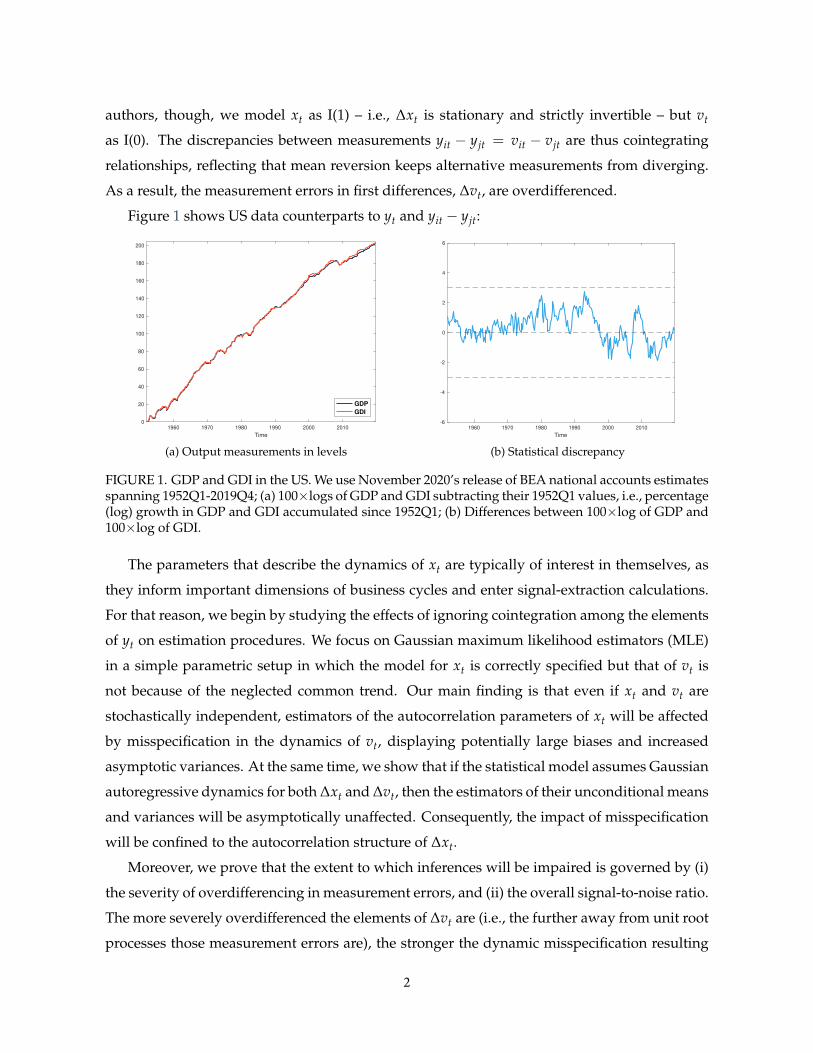
authors, though, we model xt as I(1) – i.e., ∆xt is stationary and strictly invertible – but vt

as I(0). The discrepancies between measurements yit − yjt = vit − vjt are thus cointegrating

relationships, reflecting that mean reversion keeps alternative measurements from diverging.

As a result, the measurement errors in first differences, ∆vt, are overdifferenced.

Figure 1 shows US data counterparts to yt and yit − yjt:

1960 1970 1980 1990 2000 2010

Time

0

20

40

60

80

100

120

140

160

180

200

GDP

GDI

(a) Output measurements in levels

1960 1970 1980 1990 2000 2010

Time

-6

-4

-2

0

2

4

6

(b) Statistical discrepancy

FIGURE 1. GDP and GDI in the US. We use November 2020’s release of BEA national accounts estimatesspanning 1952Q1-2019Q4; (a) 100×logs of GDP and GDI subtracting their 1952Q1 values, i.e., percentage(log) growth in GDP and GDI accumulated since 1952Q1; (b) Differences between 100×log of GDP and100×log of GDI.

The parameters that describe the dynamics of xt are typically of interest in themselves, as

they inform important dimensions of business cycles and enter signal-extraction calculations.

For that reason, we begin by studying the effects of ignoring cointegration among the elements

of yt on estimation procedures. We focus on Gaussian maximum likelihood estimators (MLE)

in a simple parametric setup in which the model for xt is correctly specified but that of vt is

not because of the neglected common trend. Our main finding is that even if xt and vt are

stochastically independent, estimators of the autocorrelation parameters of xt will be affected

by misspecification in the dynamics of vt, displaying potentially large biases and increased

asymptotic variances. At the same time, we show that if the statistical model assumes Gaussian

autoregressive dynamics for both ∆xt and ∆vt, then the estimators of their unconditional means

and variances will be asymptotically unaffected. Consequently, the impact of misspecification

will be confined to the autocorrelation structure of ∆xt.

Moreover, we prove that the extent to which inferences will be impaired is governed by (i)

the severity of overdifferencing in measurement errors, and (ii) the overall signal-to-noise ratio.

The more severely overdifferenced the elements of ∆vt are (i.e., the further away from unit root

processes those measurement errors are), the stronger the dynamic misspecification resulting

2

from the omitted common trend will be. In addition, a low degree of signal observability, which

we quantify by means of an R2 measure of the relative contribution of xt and vt to the variation

in observables, amplifies the role of incorrect modeling assumptions on vt. In the limiting case

of R2 = 1, xt is observable and misspecification in vt inconsequential.3

Prediction, filtering and smoothing of xt given data on yt – signal extraction, for short –

constitute the other main focus of our paper. Given that the uncertainty of signal extraction

calculations does not vanish in large T samples, unlike that of parameter estimators, we study

their behavior at the pseudo-true parameter values, i.e., at the probability limits of ML esti-

mators. Thus, we leverage on our estimation results to establish the suboptimality as a signal

extraction technique of the Kalman-filter-based methods that neglect the common trend.

Furthermore, we find that the effect of ignoring the common trend is substantially different

when signal extraction targets a short-run object and a long-run one. In particular, confidence

sets for a long-run object such as an average of ∆xt over a relatively large time span are highly

sensitive to even modest amounts of overdifferencing in ∆vt. This result is important because

long-run objects are relevant for answering empirical questions about slowly evolving trends

in macro variables. One example originates in the recurrent debate about growth decelera-

tion in industrialized economies (e.g., Gordon (2016)). Another instance is the secular stagna-

tion hypothesis, which postulates a downward trend in interest rates (e.g., Hansen (1939) and

Summers (2015)). Similarly, the apparent secular decline in labor shares (e.g., Kaldor (1957),

Blanchard (1997) and Karabarbounis and Neiman (2014)) provides another case in point.

On the empirical side, we fit our proposed common trend model to US data on GDP and

GDI. Through standard Kalman smoothing calculations, we obtain an improved measure of

economic activity, which we compare to other existing measures in the literature. We then use

our improved measure to assess the robustness of a variety of empirical facts on economic ac-

tivity, involving both short- and long-run objects. Our main findings are the following: (1) point

estimates of the serial correlation structure of economic activity appear robust to common trend

assumptions, (2) the same seems to be true of point estimates of the quarterly rate of growth in

GDP, but (3) our common trend model gives rise to lower signal extraction uncertainty about

economic activity than its competitors. Our third finding is conceptually important because

point estimates of latent variables cannot be justified by an appeal to consistency — uncer-

3In unreported simulation experiments, we explore the possibility that biases in parameter estimators may bereduced by means of a flexible model of the serial dependence structure of measurement errors in first differences.Specifically, we model ∆vt as a set of independent univariate AR(p) models with p large. Our analysis suggests thatbias reduction is thus possible, but at the expense of significant precision loss. Large-p, large-T double-asymptoticsin this context appear to be an interesting (but challenging) avenue for future research.

3

tainty about latent variables remains high regardless of the sample size, implying that such

estimates must be accompanied by a measure of their precision. This is particularly important

from an empirical point of view because the “putative” precision of estimates of economic ac-

tivity which do not impose a common trend is so low that no sharp conclusion can be drawn

about trends in growth from them. In contrast, our common-trend model provides noticeably

more precise inference about such long-run objects.

Of course, whether or not there is a common trend is an empirical question in its own right.

The evidence that the statistical discrepancy between US GDP and GDI, although persistent, is

mean-reverting is suggestive but not conclusive.4 Yet, the fact that, absent a common trend, the

probability of observing large deviations between different measurements tends to one, lends

strong support to our framework in the context of aggregate measurement problems.

The rest of the paper is organized as follows. In section 2 we present the basic setup. Section

3 discusses the properties of maximum likelihood estimators while section 4 is devoted to fil-

tering. We report the results of our empirical analysis in section 5. Finally, section 6 concludes.

Additional results are relegated to appendixes A, B and C.

Notation. We use ωt0 :t1to denote the sequence ωt

t1t=t0

. If ωt is a d1 × d2 array for all t, and

if it raises no confusion, we also use ωt0 :t1to denote the d1(t1 − t0 + 1)× d2 array obtained by

vertical concatenation of the terms of ωtt1t=t0

. Analogously, ψ1:N denotes the column vector

of parameters (ψ1, . . . , ψn)′. We write ET[ωt] = T−1 ∑T

t=1 ωt for the sample average of ω1:T,

E[ωt] for its population counterpart, “p−→ ” for convergence in probability and “ =⇒ ” for

weak convergence.

2 Model

In our setup, the statistical office collects N measurements yt of an unobserved scalar quantity

xt. Let vt be the vector of measurement errors so that, in first differences,

∆yt = ∆xt1N×1 + ∆vt, t = 1, . . . , T.(1)

For a sample ∆y1:T, the data generating process is given by the probability distribution P.

Assumption 1. P satisfies the following:

4This is most probably related to the low power attributed to cointegration tests.

4

(A) The time series ∆x0:T, v1,0:T, . . . , vN,0:T are cross-sectionally independent;

(B) ∆xt is a Gaussian AR(1) process: For some values µ0, ρ0 ∈ (−1, 1), σ0 > 0,

∆x0 ∼ N(µ0, σ20 ),

∆xt|∆x0:(t−1) ∼ N(

µ0 + ρ0(∆xt−1 − µ0), (1− ρ20)σ

20

), t = 1, . . . , T;

(C) vit is a Gaussian AR(1) process: For some values ρi ∈ (−1, 1], σi > 0,

vi0 ∼ N(

0,(1 + ρi)

2σ2

i

),

vit|vi,0:(t−1) ∼ N(

ρivi,t−1,(1 + ρi)

2σ2

i

), t = 1, . . . , T, i = 1, . . . , N.

Assumptions (A) and (B) are made in essentially every paper in the literature (e.g., Smith

et al. (1998), Greenaway-McGrevy (2011), Aruoba et al. (2016), and Almuzara et al. (2019)). In-

dependence between ∆xt and measurement errors rules out cyclical patterns in the statistical

discrepancy. Although potentially of substantive interest, introducing dependence between

∆xt and vt or across the vit’s complicates identification of the spectra of latent variables. Sim-

ilarly, AR(1) dynamics for ∆xt is generally agreed to be a reasonable benchmark for economic

activity data. Normality is unnecessary for most of our analysis, but since our focus is on the

modeling of measurement errors and the role of dynamic misspecification, we adopt it for ease

of exposition.

According to (B), we can regard ∆x0:T as a segment from a strictly stationary process ∆x−∞:∞,

∆xt = (1− ρ0)µ0 + ρ0∆xt−1 +

√1− ρ2

0σ0ε0t,

with ε0tiid∼ N(0, 1). We parameterize the process so that E[∆xt] = µ0 and Var(∆xt) = σ2

0 , and

its serial dependence structure is summarized by its spectral density

f0(λ) = σ20

(1− ρ20)

(1− ρ0eiλ)(1− ρ0e−iλ)= σ2

0

(∞

∑`=−∞

ρ|`|0 ei`λ

)

Assumption (C) implies ∆vit is overdifferenced, the severity of overdifferencing increasing

as ρi moves away from unity. In fact, ∆vit is a strictly noninvertible ARMA(1, 1) process, except

in the limiting case ρi = 1, when ∆vit becomes white noise. Similarly, we can view ∆vi,0:T as a

5

segment from a strictly stationary process ∆vi,−∞:∞,

∆vit = ρi∆vi,t−1 +

√(1 + ρi)

2σi∆ε it,

with ε itiid∼ N(0, 1). We have E[∆vit] = 0 and Var(∆vit) = σ2

i , and the spectral density of ∆vit is

fi(λ) = σ2i(1 + ρi)(1− eiλ)(1− e−iλ)

2(1− ρieiλ)(1− ρie

−iλ),

which vanishes at frequency λ = 0 if ρi 6= 1 – an unequivocal symptom of overdifferencing.

When ρi 6= 1 for all i, the spectral density matrix of ∆yt at λ = 0 is f0(0)1N×N . Therefore, it

is singular with finite positive diagonal, implying the cointegration (of rank N− 1) of yt. Thus,

yt is driven by a single common trend, xt, while the statistical discrepancies dij,t = yit − yjt are

cointegrating relationships.5

Henceforth, we assume the econometrician formulates a statistical model P = Pθ : θ ∈ Θwhere θ = (ϑ′, ψ′1:N)

′ with ϑ = (µ, ρ, σ)′ and Θ = Θx × Θv, Θx ⊂ R × (−1, 1) × R>0 and

Θv ⊂ RN>0. The distribution Pθ is such that

(a) The time series ∆x0:T, ∆v1,0:T, . . . , ∆vN,0:T are cross-sectionally independent;

(b) ∆x0 ∼ N(µ, σ2) and ∆xt|∆x0:(t−1) ∼ N(

µ + ρ(∆xt−1 − µ), (1− ρ2)σ2)

, t = 1, . . . , T;

(c) ∆vitiid∼ N(0, ψ2

i ), i = 1, . . . , N.

From (a) and (b) it follows that the econometrician has correctly specified the model for

∆x0:T conditional on ϑ0 = (µ0, ρ0, σ0)′ ∈ Θx, an assumption we maintain in what follows.

Similarly, σ1:N ∈ Θv. In contrast, the model for the observed data ∆y1:T is misspecified unless

ρi = 1 for all i. In effect, (c) captures the idea that the econometrician neglects the common

trend in yt caused by the mean reversion of measurement errors because she assumes that

vt = ∑tτ=1 ∆vτ + v0 is a set of N independent random walks.

To ease the comparisons, the statistical model is also parameterized so that Eθ [∆xt] = µ and

Varθ(∆xt) = σ2, where the subscript θ indicates moments of the assumed distribution, so that

the implied spectral density of ∆xt becomes

fϑ(λ) = σ2 (1− ρ2)

(1− ρeiλ)(1− ρe−iλ),

5There are N(N − 1)/2 statistical discrepancies but only N − 1 of them are linearly independent. For example,all the discrepancies with respect to a fixed measurement j form a basis of the cointegration space.

6

which coincides with f0 at ϑ = ϑ0. For measurement errors, Eθ [∆vit] = 0 and Varθ(∆vit) = ψ2i .

Importantly, the assumed spectral density matrix of ∆yt at λ = 0 is fϑ(0)1N×N + diag(ψ21:N),

which is nonsingular.

Identification. A statistical model that makes use of assumption (a) attains nonparametric

identification of the spectra of latent variables. Given a spectral density matrix f∆y for the

observables, equation (1) and assumption (a) deliver

f∆y(λ) = f∆x(λ)1N×N + diag[ f∆v(λ)] ,

where f∆x is the spectral density of ∆xt and f∆v is the N-dimensional vector of spectral densi-

ties of ∆v1t, . . . , ∆vNt. Therefore, the ij-th entry of f∆y(λ), for any i 6= j, equals f∆x(λ), which

subtracted from the diagonal of f∆y(λ) yields f∆v(λ). In fact, assumption (a) imposes overi-

dentifying restrictions on f∆y for N > 2, as it implies that the off-diagonal elements of f∆y must

be equal. Consequently, the joint probability distribution of the time series ∆xt, ∆vt is iden-

tified under Gaussianity, provided one adds some restrictions on the unconditional means of

the latent variables, which are necessary because there are N + 1 unconditional means but we

only observe N measurements. Assumption 1, for example, imposes that the expectation of all

measurement errors are zero, which is enough to identify µ0 = E[∆xt] for any N ≥ 1.

2.1 Observability of the signal: a key parameter

Measures of the relative contributions of signal and noises to variation in observables are often

important for understanding the quality of estimation and filtering in unobserved components

models. To develop such a measure, we use the idea of minimal sufficient statistic for dynamic

factor models in Fiorentini and Sentana (2019). With L the lag operator and Fi(.) the autocovari-

ance generating function of ∆vit,6 the Generalized Least Squares (GLS) estimator of ∆xt based

on the past, present and future of ∆yt is

∆yt =∑N

i=1 F−1i (L)∆yit

∑Ni=1 F−1

i (L)= ∆xt +

∑Ni=1 F−1

i (L)∆vit

∑Ni=1 F−1

i (L).

Fiorentini and Sentana (2019) show that ∆yt, a one-dimensional linear filter applied to ∆yt,

contains all relevant information about ∆xt in ∆yt, in the sense that the application of the

Kalman filter to ∆yt delivers the same predictions for ∆xt as the Kalman filter applied to ∆yt.

6That is Fj(eiλ) = f j(λ).

7

We denote the resulting error by ∆vt, and note it has variance and spectral density given by

Var(∆vt) = σ2 =(

∑Ni=1 σ−2

i

)−1and f (λ) =

(∑N

i=1 f−1i (λ)

)−1, respectively.

Fiorentini and Sentana (2019) also derive the frequency-domain analogue to ∆yt, namely

∞

∑t=−∞

∆yteiλt = ∆y(λ) = ∆x(λ) + ∑N

i=1 f−1i (λ)∆vi(λ)

∑Ni=1 f−1

i (λ)= ∆x(λ) + ∆v(λ).

In this context, we take

R2(λ) =f0(λ)

f0(λ) + f (λ),

i.e. the fraction of the variance of ∆y(λ) explained by ∆x(λ), as an indicator of the degree

of observability of the signal at frequency λ. As we shall see, this measure will reveal the

frequencies at which the effect of misspecification in measurement errors is more severe for

inferences about ∆xt. In addition, we can obtain an overall measure of observability of the

signal by simply integrating Fourier transforms over [0, 2π], which yields

R2 =σ2

0

σ20 + σ2 .

Thus, a "more observable" signal is indicated by R2(λ) and R2 closer to unity.7 In particular,

when one of the measurement error variances is zero, R2(λ) = 1 and R2 = 1.

3 Estimation

We can obtain numerically equivalent Gaussian MLEs of θ, θ, by means of two algorithms.8 The

first one exploits the Kalman filter to recursively compute the one-period ahead conditional

means and variances of observables, mt(θ) = Eθ

[∆yt

∣∣∣y1:(t−1)

]and St(θ) = Varθ

(∆yt

∣∣∣y1:(t−1)

),

t = 1, . . . , T, appearing in the log-likelihood function, so that

θ = argmaxθ∈Θ

T

∑t=1

ln pθ

(∆yt|∆y1:(t−1)

),

ln pθ

(∆yt|∆y1:(t−1)

)= −1

2

[N ln(2π) + ln |St(θ)|+ (∆yt −mt(θ))

′S−1t (θ)(∆yt −mt(θ))

].

7As an alternative, one could use the signal-noise ratios q(λ) = f0(λ)/ f (λ) and q = σ20 /σ2. Nevertheless,

R2-type measures are easier to interpret because they are bounded between 0 and 1.8For brevity, we do not discuss frequency-domain ML estimation (see, e.g., Fiorentini et al. (2018)) or Bayesian

estimation (e.g., Durbin and Koopman (2012)).

8

The second is the EM algorithm, which, for some initial θ(0), updates parameter estimates by

iterating over

θ(s) = argmaxθ∈Θ

Eθ(s−1)

[T

∑t=1

ln pϑ

(∆xt|∆x1:(t−1)

)+

T

∑t=1

N

∑i=1

ln pψi(∆vit)

∣∣∣∣∣y1:T

],

ln pϑ

(∆xt|∆x1:(t−1)

)= −1

2

[ln(

2π(1− ρ2)σ2)+

(∆xt − (1− ρ)µ− ρ∆xt−1)2

(1− ρ2)σ2

],

ln pψi(∆vit) = −

12

[ln(2πψ2

i ) +∆v2

it

ψ2i

].

The EM algorithm alternates between smoothing the so-called complete-data likelihood using

the current value θ(s−1) for expectation calculations (the E-step), and maximizing the resulting

smoothed function to yield a new value θ(s) (M-step). See Dempster et al. (1977), Ruud (1991),

and Watson and Engle (1983). If the algorithm converges, we have θ = lims→∞ θ(s).

Next, we give asymptotic approximations to the sampling distribution of maximum likeli-

hood estimators under the following set up:

Assumption 2. As T → ∞, the parameters µ0, ρ0, σ0, ρ1:N , σ1:N are held constant.

Remark. An alternative local embedding in which parameters drift in a 1/√

T-neighborhood

of a fixed value can be used with little change as long as the autoregressive roots ρ0:N are

bounded away from unity. To keep the exposition focused, though, we do not allow for local-

to-unity asymptotics for the persistence of measurement errors. A setup in which ρi = 1− $i/T

with $i held fixed would capture a situation in which the researcher is uncertain about impos-

ing cointegration because the probability that a unit-root test on the differences yit − yjt rejects

the null remains bounded between 0 and 1 as T → ∞ (see, e.g., Cavanagh (1985), Chan and

Wei (1987) and Phillips (1987)). Still, our analysis suggests that the difference between unit

roots and near unit roots is very relevant for constructing inference for long-run objects (see

subsection 4.2) but not so for estimation.

Our main estimation result, whose proof appears in appendix A, is as follows:

Theorem 1. Let µ, σ, ψ1:N be the maximum likelihood estimator from the static model (i.e., the model

that assumes (a), (b) with ρ = 0, and (c)). Similarly, let µ, ρ, σ, ψ1:N be the maximum likelihood

estimator from the dynamic model P . Then, under assumptions 1 and 2,

9

√T

µ− µ

σ− σ

ψ1:N − ψ1:N

= op(1) .

Further, for some B and V,

√T(ρ− (ρ0 + B)) =⇒ N(0, V).

Therefore, µp−→ µ0, σ

p−→ σ0 and ψip−→ σi for all i. The estimators of the unconditional

mean and variance parameters of the latent variables obtained from the static and dynamic

models are asymptotically normal, and, perhaps more surprisingly, they have the same asymp-

totic covariance matrix. The consequences of neglecting the common trend are, thus, confined

to the autocorrelation structure of ∆xt. An example in appendix B provides further intuition.

This result has many implications. First, one can estimate the model parameters with-

out loss of asymptotic precision in two steps: maximizing the static model log-likelihood for

µ, σ, ψ1:N first, and then the dynamic log-likelihood for ρ after plugging in µ, σ, ψ1:N.9 Sec-

ond, the unconditional R2 measure of signal observability is consistently estimated even if the

model is misspecified, unlike its frequency-domain counterpart. Third, the estimator of ρ0 will

typically be inconsistent and display higher asymptotic variance than the estimator from the

model that correctly imposes the common trend in levels, at least when the assumption of

normality holds because of the asymptotic efficiency of the MLE under correct specification.

We can implicitly characterize the inconsistency term B by means of the spectral condition

∫ 2π

0eiλ

(fϑ(λ)

fϑ(λ) + σ2

)2 (fϑ(λ)− f0(λ) + σ2 − f (λ)

)dλ = 0,(2)

where ϑ = (µ0, ρ0 + B, σ0), σ is defined in section 2, and

f (λ) = ∑Ni=1(1/σ2

i )2 fi(λ)

(∑Ni=1(1/σ2

i ))2

is the spectrum of ∑Ni=1(1/σ2

i )∆vit/ ∑Ni=1(1/σ2

i ), i.e., the true error in the GLS minimal sufficient

9In fact, our proof suggests that the asymptotic equivalence between static and dynamic MLEs would survivein the presence of forms of dynamic misspecification other than the one we consider in this paper, and for moregeneral dynamic models, at least as long as the latent variables follow autoregressive processes.

10

statistic for ∆xt computed under the misspecified model.

When either ρi = 1 for all i or σi = 0 for at least one i, we have that f (λ) = σ2 for all λ. As

a consequence, one can set fϑ = f0, which implies a consistent estimator of ρ0 with B = 0. By

continuity, the inconsistency term B will be small when the extent of misspecification is small

(ρi’s all close to unity) or when the observability of the signal is high (R2 close to unity). In

contrast, noticeable biases may arise when one moves away from those limiting cases, as we

illustrate in the next section.

3.1 Numerical and simulation evidence

We complement our foregoing discussion of estimation with some insights from numerical and

simulation calculations. To begin with, we compute expression (2) by numerical quadrature to

obtain the inconsistency in the estimation of ρ0 as a function of the observability of the signal

and the severity of overdifferencing. We set µ0 = 3, ρ0 = 0.5 and σ0 = 3.25.10 We also take

N = 2 and let R2 (with σ1 = σ2) and ρ1 = ρ2 vary over the interval (0, 1).

-1.5

0.9

-1

0.8

B (

asym

pto

tic b

ias)

0.7

-0.5

0.80.6

R2 (observability)

0.5

0

0.6

i (overdifferencing)

0.40.40.3

0.2 0.20.1

0

FIGURE 2. Numerical computation of asymptotic bias B in the estimation of ρ0 for different extents ofoverdifferencing ρ1 = ρ2 and signal observability R2. The true value is ρ0 = 0.5. The integral in (2) isapproximated by quadrature with a fine grid on the interval [0, 2π].

10Since they represent an affine transformation of the data, the parameters µ0 and σ0 (given R2) are irrelevant forboth B and the finite-sample behavior of the ML estimators. Nevertheless, we choose the values of these parametersto match estimates from US quarterly data on economic activity for the period 1952Q1-2019Q4, so that our simulateddata resembles the actual dataset in our empirical application. Other sample periods usually lead to differentestimates of µ0 and σ0 but leave ρ0 and measures of overdifferencing and signal observability practically unchanged.

11

We display the results for this exchangeable design in figure 2. They clearly confirm our

intuition about the roles of ρi and R2 in determining B, with the inconsistency growing quickly

as R2 decreases below 0.5 even for moderate amounts of overdifferencing. Importantly, we

always find that B ≤ 0 under the form of misspecification we analyze in this paper. The ra-

tionale is as follows. Equation (2) shows that ρ0 + B is set to match a weighted average of the

difference between fϑ and f0 + σ2 − f , which is depressed at lower frequencies compared to

the true spectrum f0 by the effect of overdifferencing. To see this, note that since fϑ is an AR(1)

spectrum, lower values of fϑ at low frequencies with σ fixed at σ0 require decreasing ρ. In

particular, at frequency λ = 0, we have fϑ(0) = (1 + ρ)/(1− ρ) which decreases with ρ and,

more generally, ∂ fϑ(λ)∂ρ = −2 fϑ(λ)

[ρ

1−ρ2 +ρ−cos(λ)

1+ρ2−2ρ cos(λ)

], which is negative for low values of λ.

Hence, plimT→∞ ρ = ρ0 + B < ρ0.

We next present simulation evidence on the finite-sample properties of the following three

estimators of θ: (i) maximum likelihood for the model in first differences (i.e., θ), (ii) the two-

step procedure suggested by theorem 1, and (iii) maximum likelihood for the model in levels.

The results are summarized in tables 1, 2 and 3. They show that the approximation in theorem

1 works very well in realistic sample sizes and setups. The correlation between θ and the two-

step estimator is virtually one, as one would expect from their asymptotic equivalence, and the

inconsistency in ρ is close to the values for B obtained from equation (2). Not surprisingly, the

model in levels outperforms its competitors, although not by much for unconditional moments.

The results for a different design in which ρi = 0, which we present in appendix C, display the

same patterns.

Remark. The behavior of B as ρi approaches unity for fixed R2 can be obtained from figure

2. Our calculations suggest that√

T|B| = o(1) when ρi = 1− $i/T for all i, and that√

T|B| =O(1) would require the alternative embedding ρi = 1− $i/

√T instead. Such an embedding

would allow us to pretest the existence of a bias in the estimation of ρ0. Although we do not

formally prove these statements, they convey a sense of the relevance of estimation biases in

applications. Note that if ∆xt were observable, the standard error of ρ for a sample of seventy

years of quarterly data (T = 280) would be roughly√(1− ρ2

0)/T ≈ 0.05. If, for example, the

data were generated from the common-trend model with parameters (ρi, R2) = (0.35, 0.85),

(ρi, R2) = (0.92, 0.50) or (ρi, R2) = (0.98, 0.30), then the estimation of the model in differences

would yield a bias of size comparable to the standard error. These values seem plausible for

a large number of applications. In fact, when R2 is 0.5 or below, values of ρi which are only

slightly below unity can already cause severe downward bias in the estimation of ρ0.

12

TABLE 1. Monte Carlo simulation for ρ1 = ρ2 = 0.85 and R2 = 0.30.

True Differences Two-step Levels

µ0 mean 3 3.001 3.001 3.002stderr 0.344 0.344 0.345

corr 1 0.998ρ0 mean 0.5 0.289 0.292 0.481

stderr 0.204 0.195 0.178corr 0.942 0.451

σ0 mean 3.25 3.233 3.194 3.204stderr 0.558 0.588 0.598

corr 0.96 0.825ρi mean 0.85 0.831

stderr 0.072σi mean 7.021 6.995 7.01 6.996

stderr 0.385 0.391 0.384

NOTES. Number of samples is nMC = 2, 000, sample size is T = 280, and parameter values are given undercolumn "True". Rows "mean" and "stderr" show mean and standard deviation across simulations of each estimator;"corr" shows the correlation with MLE in differences of the other two estimators. The bias in ρ is to be comparedwith the theoretical inconsistency B ≈ −0.23 computed from equation (2) as indicated in the text.



µ0 mean 3 3.002 3.002 3.002stderr 0.341 0.341 0.341

corr 1 0.999ρ0 mean 0.5 0.41 0.408 0.488

stderr 0.111 0.11 0.105corr 0.986 0.876

σ0 mean 3.25 3.229 3.22 3.221stderr 0.322 0.321 0.326

corr 0.979 0.954ρi mean 0.85 0.822

stderr 0.089σi mean 4.596 4.583 4.589 4.581

stderr 0.266 0.272 0.268


13



µ0 mean 3 3.001 3.002 3.001stderr 0.342 0.343 0.343

corr 0.999 0.999ρ0 mean 0.5 0.478 0.475 0.49

stderr 0.062 0.062 0.065corr 0.998 0.934

σ0 mean 3.25 3.231 3.23 3.238stderr 0.196 0.196 0.205

corr 0.999 0.934ρi mean 0.85 0.781

stderr 0.24σi mean 1.931 1.925 1.926 1.914

stderr 0.148 0.165 0.252


4 Signal extraction

In general, neglecting the common trend should negatively impact filtered and smoothed esti-

mates of the latent variables. We can identify two channels through which this happens: one

important for short-run calculations, and the other for long-run calculations. We begin with

the short-run channel, i.e., the downward bias in ρ.

Consider the filtered estimate of ∆xt,

∆xt = Eθ [∆xt|∆y1:T] .

As is well-known, the filtering error ∆xt − ∆xt is Op(1) for large T. This is in contrast to the

estimation error θ − θ, with θ = (µ0, ρ0 + B, σ0, σ′1:N)′, which is op(1). Therefore, we can ob-

tain a good approximation to the behavior of ∆xt − ∆xt if we simply abstract from estimation

uncertainty and focus on filtered estimates at pseudo-true values,

∆xt = Eθ [∆xt|∆y1:T] = µ0 +T

∑τ=1

φτ,T(∆yτ − µ01N×1),

where the conditional expectation is affine because of the normality assumptions in (b)-(c).

On the other hand, the ideal filter from a mean-square error perspective is the conditional

14

mean under the correctly specified model P,11

∆x∗t = E[∆xt|∆y1:T] = µ0 +T

∑τ=1

φ∗τ,T(∆yτ − µ01N×1).

The discrepancy between the weights φ1:T,T and φ∗1:T,T is of interest because we can decom-

pose ∆xt − ∆xt into two orthogonal components: (i) the optimal filtering error ∆x∗t − ∆xt,

whose variance cannot be reduced any further in the class of measurable functions of ∆y1:T

with bounded second moments because it is unpredictable given the past, present and future

values of y1:T, and (ii) the difference between the optimal and suboptimal filters ∆xt − ∆x∗t .

To illustrate the consequences for signal extraction of neglecting the common trend in levels,

figure 3 provides a comparison of the weights for our baseline calibration when overdifferenc-

ing is not so severe (ρ1 = ρ2 = 0.85) and the degree of observability varies from low (R2 = 0.30)

to high (R2 = 0.85). We do so for the two leading signal extraction exercises encountered in

practice: the computation of ∆xt and ∆x∗t for values of t in the middle of the sample, and for

t = T (i.e., "nowcasting").

In both cases, it is clear that the filters from misspecified models tend to assign lower

weights to nearby observations relative to what is optimal, the difference being larger the lower

R2 is. For the most part, this is explained by the fact that the suboptimal filters assume the sig-

nal to be less persistent than it actually is, as B is negative and grows in absolute value as

R2 decreases. Intuitively, the negative value of B resulting from neglecting the common trend

leads the econometrician to underestimate the information content of current data.

Naturally, when overdifferencing is more severe, so is its impact on signal extraction. To

support this claim, appendix C shows an analogous weight comparison in a design with ρ1 =

ρ2 = 0. For a given R2, more severe overdifferencing means a larger downward bias in the

estimation of the persistence of the signal, which in turn implies even more depressed weights

for informative nearby observations.

4.1 Simulation evidence (continued)

We compare the finite-sample behavior of the filters discussed above using the same simula-

tion designs as in subsection 3.1 (see tables 1-3). In each simulated sample, we first obtain

maximum likelihood estimates of both the misspecified and correctly specified models, and

then we compute the corresponding smoothed estimates of ∆xt for t ≈ T/2 and t = T. We

11The data in levels enable the use of y0 in E[∆xt|∆y1:T , y0], which dominates ∆x∗t = E[∆xt|∆y1:T ] unless ρ0 = 0.

15

-10 -8 -6 -4 -2 0 2 4 6 8 10

- t

-0.1

0

0.1

0.2

0.3

0.4

0.5

right

wrong

(a) ρ1 = ρ2 = 0.85 and R2 = 0.30 (middle)

-20 -18 -16 -14 -12 -10 -8 -6 -4 -2 0

- t

-0.1

0

0.1

0.2

0.3

0.4

0.5

right

wrong

(b) ρ1 = ρ2 = 0.85 and R2 = 0.30 (end)

-10 -8 -6 -4 -2 0 2 4 6 8 10

- t

-0.1

0

0.1

0.2

0.3

0.4

0.5

right

wrong

(c) ρ1 = ρ2 = 0.85 and R2 = 0.50 (middle)

-20 -18 -16 -14 -12 -10 -8 -6 -4 -2 0

- t

-0.1

0

0.1

0.2

0.3

0.4

0.5

right

wrong

(d) ρ1 = ρ2 = 0.85 and R2 = 0.50 (end)

-10 -8 -6 -4 -2 0 2 4 6 8 10

- t

-0.1

0

0.1

0.2

0.3

0.4

0.5

right

wrong

(e) ρ1 = ρ2 = 0.85 and R2 = 0.85 (middle)

-20 -18 -16 -14 -12 -10 -8 -6 -4 -2 0

- t

-0.1

0

0.1

0.2

0.3

0.4

0.5

right

wrong

(f) ρ1 = ρ2 = 0.85 and R2 = 0.85 (end)

FIGURE 3. Weights of Kalman smoother. Horizontal axis is τ − t; vertical axis is first entry of φτ,T (red)and φ∗τ,T (indigo). Panels (a), (c) and (e) display weights for t ≈ T/2 (middle), and panels (b), (d) and(f) for t = T (end). The filters are computed using µ0 = 3, ρ0 = 0.50, σ0 = 3.25, ρ1 = ρ2 = 0.85 anddifferent values of (with σ1 = σ2). Wrong filter uses ρ0 + B as AR root with B computed from (2).

16

present the results for those designs that set ρ1 = ρ2 = 0.85 in tables 4 and 5. Appendix C

reports additional results setting ρ1 = ρ2 = 0.

As a general rule, T = 280 seems large enough for ∆xt to provide a good approximation to

∆xt. The same is true for ∆x∗t and the filter from the correctly specified model evaluated at the

maximum likelihood estimates, which we call ∆x∗t . The main differences in precision appear

between ∆xt and ∆x∗t rather than between the filters evaluated at the ML estimates and their

limiting values.

The effect of neglecting the common trend when measurement errors are highly persistent

seems modest in our simulations, with an increase of at most 7% in root MSE relative to the op-

timal filter in low-R2 designs. However, more severe overdifferencing combined with a low R2

leads to a substantial reduction in the precision of filters, as appendix C illustrates. Therefore,

researchers should be particularly concerned about their modeling assumptions on measure-

ment error when the R2 measure we propose in the paper is 0.5 or less, something we already

saw in the estimation results.

TABLE 4. Monte Carlo simulation for ρ1 = ρ2 = 0.85 and t ≈ T/2.

∆xt ∆xt ∆x∗t ∆x∗t

R2 = 0.30 RMSE 2.594 2.57 2.532 2.467increase 0.134 0.114 0.07

R2 = 0.50 RMSE 2.119 2.095 2.118 2.078increase 0.058 0.031 0.05

R2 = 0.85 RMSE 1.204 1.19 1.237 1.191increase 0.028 0.004 0.08

NOTES. Number of samples is nMC = 2, 000 and sample size is T = 280. Columns "∆xt" and "∆xt" refer to thewrong filter at the ML estimates and pseudo true values, respectively. Columns "∆x∗t " and "∆x∗t " refer to the rightfilter at the ML estimates and true values, respectively. Root MSE and increase in MSE as a fraction of the MSE of∆x∗t are indicated for each filter and R2.

It is interesting to note that the nowcasting estimate ∆xT is less affected by misspecification

than the smoothed estimate for an observation in the middle of the sample, as one would expect

given that the sample is relatively less informative (and therefore receives smaller weights)

when filtering ∆xT.

17

TABLE 5. Monte Carlo simulation for ρ1 = ρ2 = 0.85 and t = T.


R2 = 0.30 RMSE 2.681 2.624 2.655 2.572increase 0.083 0.049 0.062

R2 = 0.50 RMSE 2.21 2.18 2.218 2.171increase 0.039 0.013 0.039

R2 = 0.85 RMSE 1.232 1.22 1.265 1.22increase 0.025 0.002 0.07


4.2 Long-run objects

Formally, by a long-run object we mean henceforth a weighted average X = ∑Tt=1 ωt∆xt, where

the weights ω1:T satisfy ‖ω1:T‖ =√

∑Tt=1 ω2

t = O(

1/√

T)

.12 Long-run objects are useful tools

to investigate trends in aggregate quantities. Therefore, they show up regularly in empirical

studies of acceleration and deceleration of growth. Compared to smoothed estimates of short-

run objects, neglecting the common trend in the level measurements affects inferences about

long-run objects though a different channel, namely, by inflating measures of their uncertainty,

such as standard errors or confidence intervals.

As in our discussion of signal extraction for short-run objects, we abstract from estimation

uncertainty by using pseudo-true parameter values for the misspecified model and true values

for the correctly specified one. Let Y = ∑Tt=1 ωt∆yt and V = ∑T

t=1 ωt∆vt for a given set of

weights ω1:T. The measurement equation (1) delivers

Y = X1N×1 + V.

We are interested in the problem of constructing a confidence interval for X. To keep the

exposition simple, we will condition on X, which effectively treats X as a fixed quantity rather

than as a latent variable.13 Theorem 1 in Müller and Watson (2017) implies that under the

12And, of course, ωt ≥ 0 and ∑Tt=1 ωt = 1. To be precise, we ask that

√Tωt = ω(t/T) where ω : [0, 1] → R is of

bounded variation and∫ 1

0 ω2(s) ds = O(1). As an example, consider writing the average growth rate of economicactivity for the 2010’s decade in a sample running from 1950 to 2019 as X with ωt ∝ 1decade(t) = 2010.

13Our model implies an unconditional distribution for X that smoothing calculations would exploit in construct-ing confidence intervals, but it appears from our simulation evidence below that this alternative approach wouldnot critically modify our results.

18

misspecified model at the pseudo-true values,14

(Y− X1N×1) |X =⇒ N[0N×1, Ω2 diag

(σ2

1:N

)],

where Ω2 =∫ ∞−∞

∣∣∣∫ 10 eiλsω(s) ds

∣∣∣2 dλ, with ω(s) =√

TωbsTc, bsTc the integer part of sT and

ω1:T the weights used to construct X, Y and V. As a consequence, a (pointwise asymptotic)

level-(1− α) confidence interval for X based on this approximation will be

CIα =

[N

∑i=1

(σ2/σ2i )Yi ±Φ−1(α)Ωσ

],

where Φ is the standard normal CDF. In contrast, under the true data generating process,

T (Y− X1N×1) |X =⇒ N[0N×1, Ω2 diag

(Σ2

1:N

)],

where Σ2i = .5σ2

i (1 + ρi)(1− ρi)−2 is the long-run variance of vit. Therefore, the level-(1− α)

confidence interval for X based on this approximation will be

CI∗α =

[N

∑i=1

(Σ2/Σ2i )Yi ±Φ−1(α)Ω

ΣT

]

with Σ2 =[∑N

i=1(1/Σ2i )]−1

. Hence, it follows that as T → ∞,

length(CI∗α)length(CIα)

=Σ

Tσ→ 0.

In other words, the confidence interval based on the misspecified model is arbitrarily long com-

pared to the optimal interval. Given that Ωσ is the standard error a researcher who believes

the misspecified model P is correct would report, our calculations suggest that "putative" mea-

sures of uncertainty of smoothed estimates of long-run objects tend to overstate the actual

uncertainty about them.15

14In fact, we only need the limit variance calculations from Müller and Watson (2017) since normality is in ourcase the result of V being a linear combination of normally distributed random variables under P and P .

15Although here we focus on a situation with no estimation uncertainty, which allows us to reduce the inferenceproblem by focusing on the sufficient statistics Y, unreported simulation experiments confirm the same patterns forKalman smoother calculations evaluated at maximum likelihood estimates.

19

5 An improved aggregate output measure

In this section, we apply our framework to the US quarterly GDP and GDI data displayed

in figure 1 with the objective of constructing a new improved measure of economic activity.

Specifically, we use the November 2020’s release of BEA national accounts estimates for the

period 1952Q1-2019Q4 and define y1t = 400× ln(GDPt) and y2t = 400× ln(GDIt) so that their

first differences ∆y1t and ∆y2t indicate the annualized (log) growth rates. The statistical dis-

crepancy, which we compute as d12,t = (y1t − y2t)/4 = 100× ln(GDPt/GDIt), is then roughly

the percentage by which GDP exceeds GDI in levels.16 Remarkably, the levels of GDP and GDI

have remained within 3% of each other for about 70 years, lending strong support to our claim

that the two measurements are cointegrated.

TABLE 6. Estimates of model parameters for US data.

Differences Two-step Levels

µ0 estimate 2.994 2.997 2.989stderr (0.338) (0.204) (0.338)

ρ0 estimate 0.488 0.485 0.499stderr (0.057) (0.048) (0.057)

σ0 estimate 3.237 3.227 3.223stderr (0.186) (0.151) (0.184)

ρ1 estimate -0.097stderr (0.272)


ρ2 estimate 0.941stderr (0.021)


NOTES. The sample period is 1952Q1-2019Q4 (T = 271). Rows "estimate" and "stderr" show point estimate andstandard error for each estimator. A subindex 1 in ρi and σi refers to GDP while a subindex 2 refers to GDI. Thepoint estimate for signal observability R2 is 0.922 and a 95% confidence interval for R2 is [0.901, 0.943].

Table 6 reports maximum likelihood estimates for both the parameters of the common trend

model P and the statistical model P we discussed in section 3. As expected from Theorem 1,

there is no significant disagreement between different estimates of the unconditional moment

parameters µ0, σ0, σ1, σ2. The estimates of our R2 measure of common trend observability are

high at about 0.92, with a small confidence interval around them. Estimates for ρ0, in turn,

16We begin the sample in 1952Q1 to coincide with the Treasury-Fed accord. As is well known, this accord es-tablished in its modern terms the separation between monetary and fiscal policies, inaugurating a period of morestable behavior of economic aggregates in comparison to the immediate aftermath of World War II. In turn, we endour sample at 2019Q4 to avoid the use of the yet provisional (and highly variable) data from 2020. Thus, all the datain our sample has been subject to at least one annual revision by the BEA.

20

are all near 0.5, with a seemingly small downward bias in the estimators from the models

that neglect the common trend. These patterns are in line with the theoretical and simulation

analysis in section 3.17 The estimates of the autoregressive coefficient ρ2 implies that the time

series of GDI’s measurement error in levels, v2t, seems stationary but highly persistent. In

contrast, we cannot reject that the GDP’s measurement error in levels, v1t, is white noise. Next,

we discuss some of the implications of these results.

Our first consideration is about the serial dependence of the statistical discrepancy, d12,t.

Figure 4, in particular, shows that our assumption of AR(1) measurement errors in levels does a

good job at replicating the autocorrelations of this variable. Although the statistical discrepancy

is highly persistent because the GDI’s measurement error in level dominates it, it is also evident

that the serial dependence steadily declines, being already fairly low after 12 quarters. We

also note that, if anything, the autocorrelations of the statistical discrepancy tend to decrease

faster in the data than in our model, although the difference is small relative to the sampling

uncertainty.

FIGURE 4. Autocorrelations of the statistical discrepancy. The solid indigo line contains the autocorre-lations implied by model P at point estimates. Shaded area is a pointwise 95% confidence interval foreach lag.

A related observation is that the model in first differences leads to an implausibly high

probability of long-run divergence between GDP and GDI in levels. To get a sense for it,

d12,T|d12,0 ∼ N(d12,0, 0.9× T) with the estimates of the dynamically misspecified model at hand.

A quick calculation indicates that the probability that today we would observe a divergence be-

17When we restrict our sample to the one used by Aruoba et al. (2016), we obtain estimates of µ0, ρ0, σ0, σ1, σ2comparable to theirs. For the subsample 1960Q1-2011Q4 that they use, the variance of the signal is slightly lower,and so is the R2 measure of common trend observability.

21

tween GDP and GDI higher than 3% is 0.99 if the two aggregate output measurements were

not cointegrated.

The second consideration refers to the impact of neglecting the common trend in levels on

inferences about parameters and latent variables. Because ∆xt is highly observable, our theo-

retical results in sections 3 and 4 lead us to expect no significant divergence between the models

in differences and in levels with regards to maximum likelihood estimates and smoothed esti-

mates of what we have called short-run objects. We have already confirmed the similarity of

the estimates in table 6. In turn, figure 5 confirms our results for the smoothed estimates of ∆xt,

as one can hardly distinguish one model from the other in terms of the conditional mean and

variance of ∆xt given ∆y1:T.18

(a) Model in differences (b) Model in levels

FIGURE 5. Smoothed estimates of ∆xt (short-run object). The solid blue line represents the smoothedestimates and the shaded area represents 95% confidence intervals (pointwise for each t).

Nevertheless, the fact that GDP’s measurement error is essentially white noise does affect

inferences about long-run objects. Figure 6 illustrates this feature with the 8-year moving aver-

ages of ∆xt. We take overlapping 8-year intervals for the purposes of averaging out the typical

business-cycle periodicity.19 As expected from our results in section 4.2, there is substantially

less uncertainty for the model that exploits the common trend. Specifically, the average length

of the confidence intervals is 1% for the model in differences and 0.2% for the model in levels.

This reduced uncertainty is particularly important for assessing changes in aggregate trends,

as such changes are typically small.

Finally, note that our trend estimates track far more closely 8-year moving averages of GDP

18Nevertheless, pointwise confidence intervals are shorter for the model that imposes the common trend: theiraverage length is 3.5% (in annualized growth) for the model in differences against 3% for the model in levels.

19In this respect, we follow Müller and Watson (2008) but similar patterns arise when we use 5- or 10-year inter-vals instead.

22

(a) Model in differences (b) Model in levels

FIGURE 6. Smoothed estimates of h−1 ∑h`=1 ∆xt−`+1 (h = 32, long-run object). Solid blue line represents

the smoothed estimates and shaded area represents 99% confidence intervals (pointwise for each t).

growth than those of GDI, which is again explained by the low persistence of v1t. Therefore,

we may conclude that empirical patterns about economic activity previously obtained from

low-frequency averages of GDP are robust to the presence of measurement error in view of the

small degree of filter uncertainty implied by our model.

6 Conclusion

From a practical point of view, the first lesson we can extract from our study regarding ag-

gregate output measurement is that the need to account for a common trend in levels hinges

critically on how important measurement errors are in driving observable variation. For quar-

terly or annual data, measurement errors might be small; for monthly and, particularly, for

high-frequency data the opposite should be expected. Although no direct measure of economic

activity exists at the monthly frequency, nowcasting exercises at high frequencies typically con-

tain larger amounts of measurement errors as they feed on noisier, more preliminary, input

data. The nature of what is being measured matters too as different economic concepts have

different associated degrees of noisiness. For example, it is not the same to look at the quarterly

growth rate of GDP than to look at its quinquennial analogue. As a practical prescription, we

recommend the estimation of the R2 measure of trend observability we develop in the paper.

We also strongly urge researchers to always impose a common trend, especially when the R2

turns out low – an R2 below 0.5 should be cause of concern.

Moreover, our econometric analysis yields several insights which are of theoretical interest.

First, we prove that estimators of unconditional first and second moments under the misspeci-

23

fied model are asymptotically equivalent to static model estimators. Second, we show that the

form of misspecification studied in this paper causes a downward bias in the estimated persis-

tence of the signal. And third, we highlight that the misspecified model will tend to overstate

uncertainty of smoothed estimates of latent variables, and dramatically so for long-run objects.

Although we derive these results in a simplified parametric model, our methods of analysis

allow easy extension to more general setups. In particular, our analysis may be adapted to

dynamic factor models with nontrivial cross-sectional dimensions – models in which the usual

data preprocessing may likely lead to overdifferencing.

On the empirical side, we construct a new improved measure of US aggregate output from

GDP and GDI data. Unlike existing signal-extraction measures, ours allows GDP and GDI’s

measurement errors in levels to mean-revert, a property that fits well with the data. Still, given

that signal observability is high in this application, our estimates of the parameters of the dy-

namics of output growth are not affected much by ignoring the stationarity of the measure-

ment errors. Nevertheless, our common trend approach delivers noticeable reductions in the

implied uncertainty of smoothed estimates of true output growth. Specifically, measured in

terms of root mean square errors, the reductions are around 15% for short-run objects and 80%

for long-run ones.

One important practical issue that we have neglected in this paper is the regular updating

of the GDP and GDI measures by the BEA. In Almuzara et al. (2021), we are currently exploring

this relevant research avenue within the common trends framework of this paper.

A Proof of theorem 1

Our proof relies heavily on a generalization of Louis (1982) score formula, which we call EM

principle, formalized in e.g. Almuzara et al. (2019, th. 1). Consider the functions

gµ(θ) =√

T(

ET[∆xt − ρ∆xt−1]

1− ρ− µ

),

gρ(θ) =√

TET

[(∆xt−1 − µ)(∆xt − µ)− ρ(∆xt−1 − µ)2

],(A.1)

gσ(θ) =√

T

ET

[((∆xt − µ)− ρ(∆xt−1 − µ))2

]1− ρ2 − σ2

,

gψi(θ) =

√T(

ET

[∆v2

it

]− ψ2

i

), i = 1, . . . , N.

24

These are proportional to the scaled average scores of the complete-data log-likelihood for

the misspecified model. Maximum likelihood estimates θ are characterized by the first-order

necessary conditions

Eθ

[gµ(θ)

∣∣∣∆y1:T

]= Eθ

[gρ(θ)

∣∣∣∆y1:T

]= Eθ

[gσ(θ)

∣∣∆y1:T]= Eθ

[gψi

(θ)∣∣∣∆y1:T

]= 0.

Define the auxiliary functions

gµ(θ) =√

T (ET[∆xt]− µ) ,

gσ(θ) =√

T(

ET

[(∆xt − µ)2

]− σ2

),

and note that the maximum likelihood estimates for the static model θ (i.e., the restricted max-

imum likelihood estimates subject to ρ = 0) satisfy

Eθ

[gµ(θ)

∣∣∣∆y1:T

]= Eθ

[gσ(θ)

∣∣∆y1:T]= Eθ

[gψi

(θ)∣∣∣∆y1:T

]= 0.(A.2)

The first lemma will allow us to replace gµ and gσ by the much simpler gµ and gσ.

Lemma 1. Let θ be the maximum likelihood estimator for the misspecified model. Under assumptions 1

and 2,

Eθ

[gµ(θ)

∣∣∣∆y1:T

]= Eθ

[gµ(θ)

∣∣∣∆y1:T

]+ op(1) and Eθ

[gσ(θ)

∣∣∆y1:T]= Eθ

[gσ(θ)

∣∣∆y1:T]+ op(1) .

Proof. For any θ ∈ Θ,

gµ(θ)− gµ(θ) =ρ(∆xT − ∆x0)

(1− ρ)√

T.

One can then show that Eθ [∆x0|∆y1:T] = Op(1) and Eθ [∆xT|∆y1:T] = Op(1), which leads to

Eθ

[gµ(θ)− gµ(θ)

∣∣∣∆y1:T

]= Op

(1/√

T)

.

In particular, this implies that Eθ

[gµ(θ)− gµ(θ)

∣∣∣∆y1:T

]= op(1).

Turning to the score function with respect to σ, for any θ ∈ Θ,

gσ(θ) +2ρ

1− ρ2 gρ(θ)− gσ(θ) =ρ2((∆xT − µ)2 − (∆x0 − µ)2)

(1− ρ2)√

T.

25

Since Eθ

[(∆x0)

2∣∣∣∆y1:T

]= Op(1) and Eθ

[(∆xT)

2∣∣∣∆y1:T

]= Op(1),

Eθ

[gσ(θ) +

2ρ

1− ρ2 gρ(θ)− gσ(θ)

∣∣∣∣∣∆y1:T

]= Op

(1/√

T)

.

And since Eθ

[gρ(θ)

∣∣∣∆y1:T

]= 0, we finally get Eθ

[gσ(θ)− gσ(θ)

∣∣∆y1:T]= op(1).

Remark. A subtlety in the previous proof is that order-in-probability statements refer to P

while expectations refer to Pθ . For the sake of brevity, we omit the proof that this difference is

inconsequential.

Let θρ=0 be the parameter vector θ in which we set ρ = 0. In an abuse of notation, we will

also occasionally identify θρ=0 with the subvector that excludes the ρ = 0 component. For the

proof of lemma 2, the following remark will be useful:

Remark. Sample spaces of ∆y1:T, ∆x0:T, and ∆v1:T are Y = RNT, X = R

T+1, and V = RNT.

Probability distributions P and Pθ , θ ∈ Θ, may be taken to be measures on the Borel sets of

X × V with probability statements about ∆y1:T interpreted by means of the inverse image of

the mapping in (1). The measure P and the model P are then dominated by Lebesgue measure

λ on the Borel sets of X × V . Consequently, densities exist by the Radon-Nikodym theorem.

In contrast, conditional distributions of ∆x0:T and ∆v1:T given ∆y1:T implied by P and P are

dominated by the σ-finite measure λ∆y1:Ton the Borel sets of the hyperplane defined by (1) for

fixed ∆y1:T, rather than by P . Therefore, conditional densities exist with respect to λ∆y1:Tin that

case too.

Lemma 2. Under assumptions 1 and 2,

√T(

Eθ [ET[∆xt]|∆y1:T]−Eθρ=0[ET[∆xt]|∆y1:T]

)= op(1) ,

√T(

Eθ

[ET

[∆x2

t

]∣∣∣∆y1:T

]−Eθρ=0

[ET

[∆x2

t

]∣∣∣∆y1:T

])= op(1) ,

√T(

Eθ

[ET

[∆v2

it

]∣∣∣∆y1:T

]−Eθρ=0

[ET

[∆v2

it

]∣∣∣∆y1:T

])= op(1) , i = 1, . . . , N.

Proof. Let x denote the latent variables ∆x0:T, v1:N,1:T and y the observables ∆y1:T. Under

the restriction ρ = 0, the model for x has density

pη(x) = b exp[T · (η′S(x)− a(η))

]26

with respect to measure λ. Similarly, the density of x given y is an exponential family with

density

pη(x|y) = b exp[T · (η′S(x)− a(η|y))

]with respect to measure λy. Measures λ and λy are defined in the remark above, b is a constant,

η = η(µ, σ, ψ1:N) is a function of the original parameters, a(·) and a(·|y) are functions of η, and

the sufficient statistics are S(x) = ET

[(∆xt, ∆x2

t , ∆v21t, . . . , ∆v2

Nt)′].

Define S = Eθ [S(x)] and note that if x is such that S(x) = S, then the densities pη(x) and

pη(x|y) are maximized at η = η(µ, σ, ψ1:N).

In addition,

S =∂a(η)

∂η=

∂a(η|y)∂η

= Eθρ=0,[S(x)|y]

where this statement follows from well-known properties of exponential families (Jørgensen

and Labouriau, 2012, Th. 1.17 and 1.18). Since Eθ [S(x)|y] = S + op

(1/√

T)

by virtue of lemma

1), the current lemma immediately follows.

The rest of the argument for the equivalence between θρ=0 and θρ=0 is quite standard.

Specifically, if G collects the static model estimating equations (A.2) (suitably scaled by sample

size), and θρ=0 denotes the (common) probability limit of the two estimators, then a standard

Taylor expansion gives

op(1) = G(θρ=0)− G(θρ=0) =[

H(θρ=0) + op(1)]×√

T(θρ=0 − θρ=0),

where H(θρ=0) is a fixed nonsingular matrix, which in turn implies√

T(θρ=0 − θρ=0) = op(1).

From (A.1) and the asymptotic equivalence result, after some algebraic manipulations we

obtain the following representation of the maximum likelihood estimator for ρ,

ρ =Eθ [ET[(∆xt−1 − µ)(∆xt − µ)]|∆y1:T]

σ20

+ op

(1√T

).

This equation expresses ρ as the ratio between a smoothed (average) covariance and a variance.

Further developing the smoothed covariance one can establish the spectral condition (2) that

we use to characterize the pseudo-true value of ρ.

27

B AR(1) example

Consider the following stationary Gaussian AR(1) model:

yt = c + ryt−1 + ut,

utiid∼ N(0, s2)

The information matrix for the MLE of α = (c, r, s2) assuming yt observable is

I(α) =

s−2 s−2µ 0

s−2µ s−2(µ2 + σ2) 0

0 0 12 s−4

,

where µ = E[yt−1] = c/(1− r) and σ2 = Var(yt−1) = s2/(1− r2).

Consider the following reparameterization: α 7→ θ = (µ, ρ, σ2) where

µ =c

1− r,

ρ = r,

σ2 =s2

1− r2 ,

whose inverse is given by

c = µ(1− ρ),

r = ρ,

s2 = (1− ρ2)σ2.

Effectively, this amounts to re-writing the Gaussian AR(1) process above as

(yt − µ) = ρ(yt−1 − µ) +

√σ2(1− ρ2)εt,

εtiid∼ N(0, 1).

28

The Jacobian of the inverse transformation is

∂α

∂θ′=

1− ρ −µ 0

0 1 0

0 −2ρσ2 1− ρ2

=

1− r − c

1−r 0

0 1 0

0 − 2rs2

1−r2 1− r2

A straightforward application of the chain rule for derivatives implies that the information

matrix of the transformed parameters θ will be

I(θ) = ∂α′

∂θI(α) ∂α

∂θ′=

1s2 (r− 1)2 0 0

0 1

(r2−1)2

(r2 + 1

)− 1

s2 r

0 − 1s2 r 1

2s4

(r2 − 1

)2

whose inverse is

I−1(θ) =

s2

(1−r)2 0 0

0 1− r2 2s2 r1−r2

0 2s2 r1−r2 2s4 (1+r2)

(1−r2)3

Given that the spectral density of yt at frequency 0 is s2/(1− r)2, it is clear that the dynamic

estimator of µ has the same asymptotic variance as the sample mean of xt, which coincides

with the ML estimator of µ that erroneously imposes that r = 0.

To find out the asymptotic variance of the sample variance, we need to obtain the autocorre-

lation structure of y2t , which, given the Gaussian nature of the process, will be that of an AR(1)

with autoregressive coefficient r2. In addition, given that

(yt − µ)2 = r2(yt−1 − µ)2 + s2ε2t + 2rs(yt−1 − µ)εt,

the innovation variance of this autoregression would be

Var(

s2ε2t + 2rs(yt−1 − µ)εt

)= 2s4 + 4r2s2 s2

(1− r2)= 2s4

(1 +

2r2

(1− r2)

)= 2s4

(1 + r2

)(1− r2)

,

29

so the spectral density of (yt − µ)2 at the frequency 0 will be

2s4

(1 + r2

)(1− r2)

1

(1− r2)2 .

This confirms that the dynamic estimator of σ2 has the same asymptotic variance as the sample

variance of yt, which coincides with the ML estimator of σ2 that erroneously assumes that r = 0.

C Additional simulation results

Simulation results for designs similar to the ones displayed in the text but with ρ1 = ρ2 = 0

(instead of ρ1 = ρ2 = 0.85) are collected below. In particular, we generate simulated data from

the distribution P with µ0 = 3, ρ0 = 0.5 and σ0 = 3.25. We also take N = 2 and let R2 (with

σ1 = σ2) and ρ1 = ρ2 vary over the interval (0, 1).

Tables C.1, C.2 and C.3 are analogous to tables 1, 2 and 3 in the text and summarize esti-

mation results. Figure C.1 is analogous to figure 3 in the text and contains weight comparisons

for smoothed estimates of the signal. Finally, tables C.4 and C.5 are analogous to tables 4 and 5

and describe the performance of filtering procedures. Please, refer to the text for further detail.

TABLE C.1. Monte Carlo simulation for ρ1 = ρ2 = 0 and R2 = 0.30.


µ0 mean 3 3.003 3.003 3.003stderr 0.34 0.341 0.34

corr 1 1ρ0 mean 0.5 -0.487 -0.496 0.466

stderr 0.148 0.158 0.132corr 0.663 -0.086

σ0 mean 3.25 3.393 3.194 3.298stderr 0.55 0.639 0.364

corr 0.917 0.587ρi mean 0 0

stderr 0.087σi mean 7.021 6.91 6.994 6.972

stderr 0.433 0.451 0.405

NOTES. Number of samples is nMC = 2, 000 and sample size is T = 280. The bias in ρ is to be compared with thetheoretical inconsistency B ≈ −1.01 computed from equation (2) as indicated in the text.

30



µ0 mean 3 3.002 3.002 3.002stderr 0.341 0.341 0.341

corr 1 1ρ0 mean 0.5 0.007 -0.001 0.479

stderr 0.208 0.186 0.096corr 0.933 0.43

σ0 mean 3.25 3.192 3.218 3.255stderr 0.369 0.33 0.255

corr 0.942 0.788ρi mean 0 -0.002

stderr 0.098σi mean 4.596 4.601 4.587 4.572

stderr 0.321 0.309 0.283




µ0 mean 3 3 3.001 3stderr 0.342 0.342 0.342

corr 0.999 0.999ρ0 mean 0.5 0.414 0.414 0.489

stderr 0.071 0.071 0.064corr 1 0.95

σ0 mean 3.25 3.228 3.231 3.236stderr 0.19 0.19 0.188

corr 1 0.986ρi mean 0 -0.013

stderr 0.144σi mean 1.931 1.926 1.922 1.917

stderr 0.155 0.158 0.158


31

-10 -8 -6 -4 -2 0 2 4 6 8 10

- t

-0.1

0

0.1

0.2

0.3

0.4

0.5

right

wrong

(a) ρ1 = ρ2 = 0 and R2 = 0.30 (middle)

-20 -18 -16 -14 -12 -10 -8 -6 -4 -2 0

- t

-0.1

0

0.1

0.2

0.3

0.4

0.5

right

wrong

(b) ρ1 = ρ2 = 0 and R2 = 0.30 (end)

-10 -8 -6 -4 -2 0 2 4 6 8 10

- t

-0.1

0

0.1

0.2

0.3

0.4

0.5

right

wrong

(c) ρ1 = ρ2 = 0 and R2 = 0.50 (middle)

-20 -18 -16 -14 -12 -10 -8 -6 -4 -2 0

- t

-0.1

0

0.1

0.2

0.3

0.4

0.5

right

wrong

(d) ρ1 = ρ2 = 0 and R2 = 0.50 (end)

-10 -8 -6 -4 -2 0 2 4 6 8 10

- t

-0.1

0

0.1

0.2

0.3

0.4

0.5

right

wrong

(e) ρ1 = ρ2 = 0 and R2 = 0.85 (middle)

-20 -18 -16 -14 -12 -10 -8 -6 -4 -2 0

- t

-0.1

0

0.1

0.2

0.3

0.4

0.5

right

wrong

(f) ρ1 = ρ2 = 0 and R2 = 0.85 (end)

FIGURE C.1. Weights of Kalman smoother. Horizontal axis is τ − t; vertical axis is first entry of φτ,T(red) and φ∗τ,T (indigo). Panels (a), (c) and (e) display weights for t ≈ T/2 (middle), and panels (b), (d)and (f) for t = T (end). The filters are computed using µ0 = 3, ρ0 = 0.50, σ0 = 3.25, ρ1 = ρ2 = 0 anddifferent values of R2 (with σ1 = σ2). Wrong filter uses ρ0 + B as AR root with B computed from (2).

32

TABLE C.4. Monte Carlo simulation for ρ1 = ρ2 = 0 and t ≈ T/2.


R2 = 0.30 RMSE 3.192 3.216 1.994 1.964increase 1.729 1.763 0.044

R2 = 0.50 RMSE 2.246 2.074 1.712 1.684increase 0.848 0.571 0.034

R2 = 0.85 RMSE 1.118 1.104 1.093 1.058increase 0.134 0.108 0.047


TABLE C.5. Monte Carlo simulation for ρ1 = ρ2 = 0 and t = T.


R2 = 0.30 RMSE 2.998 2.957 2.356 2.325increase 0.736 0.685 0.031

R2 = 0.50 RMSE 2.254 2.154 1.973 1.954increase 0.386 0.254 0.024

R2 = 0.85 RMSE 1.175 1.163 1.152 1.139increase 0.081 0.056 0.031


33

References

ALMUZARA, M., D. AMENGUAL, G. FIORENTINI, AND E. SENTANA (2021): “GDP solera: The

ideal vintage mix.” Working paper.

ALMUZARA, M., D. AMENGUAL, AND E. SENTANA (2019): “Normality tests for latent vari-

ables.” Quantitative Economics, 10, 981–1017.

ARUOBA, S. B., F. X. DIEBOLD, J. NALEWAIK, F. SCHORFHEIDE, AND D. SONG (2016): “Im-

proving GDP measurement: A measurement-error perspective.” Journal of Econometrics, 191,

384–397.

BLANCHARD, O. J. (1997): “The medium run.” Brookings Papers on Economic Activity, 28, 89–158.

CAVANAGH, C. L. (1985): “Roots local to unity.” Harvard university manuscript.

CHAN, N. H. AND C. Z. WEI (1987): “Asymptotic inference for nearly nonstationary AR(1)

processes.” Annals of Statistics, 15, 1050–1063.

DEMPSTER, A., N. LAIRD, AND D. RUBIN (1977): “Maximum likelihood from incomplete data

via the EM algorithm.” Journal of the Royal Statistical Society, Series B, 39, 1–38.

DURBIN, J. AND S. J. KOOPMAN (2012): Time Series Analysis by State Space Methods, Oxford

University Press, second ed.

FIORENTINI, G., A. GALESI, AND E. SENTANA (2018): “A spectral EM algorithm for dynamic

factor models,” Journal of Econometrics, 205, 249–279.

FIORENTINI, G. AND E. SENTANA (2019): “Dynamic specification tests for dynamic factor mod-

els.” Journal of Applied Econometrics, 34, 325–346.

GORDON, R. J. (2016): “Perspectives on the rise and fall of American growth.” American Eco-

nomic Review: Papers and Proceedings, 106, 72–76.

GREENAWAY-MCGREVY, R. (2011): “Is GDP or GDI a better measure of output? A statistical

approach.” Bureau of Economic Analysis Working Paper 2011–08.

GRIMM, B. T. (2007): “The statistical discrepancy.” Bureau of Economic Analysis Paper 007.

HANSEN, A. (1939): “Economic progress and declining population growth.” American Economic

Review, 29, 1–15.

34

JØRGENSEN, B. AND R. LABOURIAU (2012): Exponential Families and Theoretical Inference.

KALDOR, N. (1957): “A model of economic growth.” Economic Journal, 67, 591–624.

KARABARBOUNIS, L. AND B. NEIMAN (2014): “The global decline of the labor share.” Quarterly

Journal of Economics, 129, 61–103.

LANDEFELD, J. S., E. P. SESKIN, AND B. M. FRAUMENI (2008): “Taking the pulse of the econ-

omy: measuring GDP.” Journal of Economic Perspectives, 22, 193–216.

LOUIS, T. A. (1982): “Finding the observed information matrix when using the EM algorithm.”

Journal of the Royal Statistical Society, Series B, 44, 226–233.

MÜLLER, U. K. AND M. W. WATSON (2008): “Testing models of low-frequency variability.”

Econometrica, 76, 979–1016.

——— (2017): “Low-frequency econometrics.” in Advances in Economics and Econometrics:

Eleventh World Congress of the Econometric Society, ed. by B. Honoré, A. Pakes, M. Piazzesi,

and L. Samuelson, Cambridge University Press, vol. 2.

NALEWAIK, J. (2010): “The income- and expenditure-side measures of output growth,” Brook-

ings Papers on Economic Activity, 1, 71–106.

——— (2011): “The income- and expenditure-side measures of output growth – an update

through 2011Q2.” Brookings Papers on Economic Activity, 2, 385–402.

PHILLIPS, P. C. B. (1987): “Towards a unified asymptotic theory for autoregression.” Biometrika,

74, 535–547.

RUUD, P. (1991): “Extensions of estimation methods using the EM algorithm.” Journal of Econo-

metrics, 49, 305–341.

SMITH, R. J., M. R. WEALE, AND S. E. SATCHELL (1998): “Measurement error with accounting

constraints: Point and interval estimation for latent data with an application to U.K. gross

domestic product.” Review of Economic Studies, 65, 109–134.

STONE, R., D. G. CHAMPERNOWNE, AND J. E. MEADE (1942): “The precision of national in-

come estimates.” Review of Economic Studies, 9, 111–125.

SUMMERS, L. H. (2015): “Demand side secular stagnation.” American Economic Review: Papers

and Proceedings, 105, 60–65.

35

WATSON, M. W. AND R. F. ENGLE (1983): “Alternative algorithms for estimation of dynamic

MIMIC models, factor, and time varying coefficient regression models.” Journal of Economet-

rics, 23, 385–400.

WEALE, M. (1992): “Estimation of data measured with error and subject to linear restrictions,”

Journal of Applied Econometrics, 7, 167–174.

36

no. 962 a common trend approach

Documents