no. 538 estimation and asymptotic theory for a new class ... · alvaro veiga marcelo c. medeiros...

No. 538

Estimation and asymptotic theory for a new class of mixture models

Eduardo F. Mendes

Alvaro Veiga Marcelo C. Medeiros

TEXTO PARA DISCUSSÃO

DEPARTAMENTO DE ECONOMIA www.econ.puc-rio.br

ESTIMATION AND ASYMPTOTIC THEORYFOR A NEW CLASS OF MIXTURE MODELS

Eduardo F. Mendes

Department of Statistics, Northwestern University, Evanston, IL

E-mail: [email protected]

Alvaro Veiga

Department of Electrical Engineering, Pontifical Catholic University of Rio de Janeiro


Marcelo C. Medeiros

Department of Economics, Pontifical Catholic University of Rio de Janeiro


ABSTRACT

In this paper a new model of mixture of distributions is proposed, where the mixing struc-

ture is determined by a smooth transition tree architecture. The tree structure yields a

model that is simpler, and in some cases more interpretable,than previous proposals in

the literature. Based on the Expectation-Maximization (EM)algorithm a quasi-maximum

likelihood estimator is derived and its asymptotic properties are derived under mild reg-

ularity conditions. In addition, a specific-to-general model building strategy is proposed

in order to avoid possible identification problems. Both the estimation procedure and the

model building strategy are evaluated in a Monte Carlo experiment. The approximation

capabilities of the model is also analyzed in a simulation experiment. Finally, applications

with real datasets are considered.

KEYWORDS: Mixture models, smooth transition, regression tree, conditional distribution.1

2 ESTIMATION AND ASYMPTOTIC THEORY FOR A NEW CLASS OF MIXTUREMODELS

1. INTRODUCTION

Recent years have witnessed a vast development of nonlinear time series techniques

(Tong 1990, Granger and Terasvirta 1993). From a parametric point of view, the Smooth

Transition (Auto-)Regression, ST(A)R, proposed by Chan and Tong (1986)1 and further de-

veloped by Luukkonen, Saikkonen and Terasvirta (1988) and Terasvirta (1994), has found a

number of successful applications; see van Dijk, Terasvirta and Franses (2002) for a review.

In the time series literature, the STAR model is a natural generalization of the Threshold

Autoregressive (TAR) models pioneered by Tong (1978) and Tong and Lim (1980).

On the other hand, nonparametric models that do not make assumptions about the para-

metric form of the functional relationship between the variables to be modeled have be-

come widely applicable due to computational advances (Hardle 1990, Hardle, Lutkepohl

and Chen 1997, Fan and Yao 2003). Another class of models, the flexible functional forms,

offers an alternative that leaves the functional form of therelationship partially unspecified.

While these models do contain parameters, often a large number of them, the parameters

are not globally identified. Identification, if achieved, islocal at best without imposing re-

strictions on the parameters. Usually, the parameters are not interpretable as they often are

in parametric models. In most cases, these models are interpreted as nonparametric sieve

(or series) approximations (Chen and Shen 1998).

The neural network (NN) model is a prominent example of such aflexible functional

form. Although the NN model can be interpreted as a parametric alternative (Kuan and

White 1994, Trapletti, Leisch and Hornik 2000, Medeiros, Terasvirta and Rech 2006), its

use in applied work is generally motivated by the mathematical result stating that, under

mild regularity conditions, a NN model is capable of approximating any Borel-measurable

function to any given degree of accuracy; see, for instance,Hornik, Stinchombe and White

(1990), Gallant and White (1992), and Chen and White (1998).

1Chan and Tong (1986) called the model Smooth Threshold Auto-regression.

ESTIMATION AND ASYMPTOTIC THEORY FOR A NEW CLASS OF MIXTURE MODELS 3

The above mentioned models aim to describe the conditional mean of the series. In terms

of the conditional variance, Engle’s (1982) Autoregressive Conditional Heteroskedastic-

ity (ARCH) model, Bollerslev’s (1986) Generalized ARCH (GARCH) specification, and

Taylor´s (1986) Stochastic Volatility (SV) model are the most popular alternatives for

capturing time-varying volatility, and have motivated a myriad of extensions (Poon and

Granger 2003, McAleer 2005, Andersen, Bollerslev and Diebold 2006).

However, when the attempt is to model the entire conditionaldistribution, the mixture-

of-experts (ME) proposed by Jacobs, Jordan, Nowlan and Hinton (1991) becomes a viable

alternative. The core idea is to have a family of models, which is flexible enough to capture

not only the nonlinearities in the conditional mean, but also to capture other complexities

in the conditional distribution. The model is based on the ideas of Nowlan (1990), viewing

competitive adaptation in unsupervised learning as an attempt to fit a mixture of simple

probability distributions. Jordan and Jacobs (1994) proposed the hierarchical mixture-of-

experts (HME). Applications of ME and HME models in time series are given by Weigend,

Mangeas and Srivastava (1995) and Huerta, Jiang, and Tanner(2001,2003). Recently, Car-

valho and Tanner (2005a) proposed the mixture of generalized linear time series models and

derived several asymptotic results. It would worth mentioning the Mixture Autoregressive

(MAR) model proposed by Wong and Li (2000,2001).

In this paper we contribute to the literature by proposing a new class of mixture of mod-

els that is based on regression-trees with smooth splits. Our proposal has the advantage

of being flexible but less complex than the HME specification,providing possible inter-

pretation for the final estimated model. Furthermore, a simple model building strategy has

been developed and Monte Carlo simulations show that it workswell in small samples. A

quasi-maximum likelihood estimator (QMLE) is described and its asymptotic properties

are analyzed.


The paper proceeds as follows. In Section 2 a brief review of the literature on mixture

of models for time series is presented. Our proposal is presented in Section 3. In Section

4, parameter estimation and the asymptotic theory are considered. The modeling cycle is

described in Section 5. Simulations are shown in Section 6, and Section 7 presents some

examples with actual data. Finally, Section 8 concludes. All technical proofs are relegated

to the appendix.

2. MIXTURE OF MODELS: A BRIEF REVIEW OF THE L ITERATURE

In this section we present the class of models considered in this paper.

DEFINITION 1. The conditional probability density function (p.d.f.),f(yt|xt;θ), of a ran-

dom variableyt is a Mixture of Models withK basis distributions if

(1) f(yt|xt;θ) =K∑

i=1

gi(xt;θi)πi(yt|xt;ψi),

wherext ∈ Rq is a vector of covariates,θ = [θ′1, . . . ,θ′K ,ψ

′1, . . . ,ψ

′K ]

′ is a parameter

vector,πi(yt|xt;ψi) is some known parametric family of distributions (basis distributions),

indexed by the vector of parametersψi, andgi(xt;θi) ∈ [0, 1] is the weight function.

If yt is distributed as in (1), then

E[yt|xt] =K∑

i=1

gi(xt;θi)Eπi[yt|xt;ψi] and V[yt|xt] =

K∑

i=1

g2i (xt;θi)Vπi

[yt|xt;ψi],

whereEπiandVπi

are the expected value and the variance taken with respect toπi.

The simplest model belonging to this class is the TAR model, where a threshold vari-

able controls the switching between different local Gaussian linear models. An indicator

variable defines which local model is active and only one model is active each time. The

conditional p.d.f. remains Gaussian and the conditional moments do not depend on the

covariates. Many models have been proposed to overcome these limitations. The MAR


model of Wong and Li (2000) uses a mixture of Gaussian distributions with static weights.

However, this model is still limited because the weights do not vary across time (or with the

covariate vector). Wong and Li (1999) suggest a generalization called a generalized mix-

ture of autoregressive model (GMARX). This generalization considers only two Gaussian

local models and the weights are given by a logistic equation. The GMARX model has

a limited number of local models. The ME model of Jacobs et al.(1991) describes the

conditional distribution using gated NNs to switch betweenlocal nonlinear models. This

specification though very flexible, has a high number of parameters and is very hard to

interpret, specify, and estimate. On the other hand, the HMEis a tree-structured mixture of

generalized linear models, where the weights are given by a product of multinomial logit

functions. Each node of the tree can have any number of splits, hence the specification

and estimation of the model are also demanding. Furthermore, for the most general model

there are no results that guarantee consistency of the estimators. Finally, the model is not

completely interpretable once the subdivisions of the space are done by hyperplanes which,

in turn, are not necessarily interpretable.

To overcome some of the drawbacks caused by a profligate parametrization, Zeevi, Meir

and Adler (1998) proposed the mixture autoregressive (MixAR) and Carvalho and Tanner

(2005b) considered the mixture of generalized experts, which are simplifications of the

HME model. In both cases the weights are given by a multinomial logit function. Proba-

bilistic properties and approximation results were provedfor both models; see Zeevi et al.

(1998), Carvalho and Tanner (2005a) and Carvalho and Skoulakis (2004).

The model proposed in this paper combines the simplicity of the decision trees with the

flexibility of the mixture of models. However, our model is simpler, is less parameterized,

is more easily interpretable and the model building strategy is well defined. The tree-

structured mixture of models has a binary tree as the decision structure and the decision

frontier is not a linear combination of the covariates, justone of the covariates each time.


3. MODEL PRESENTATION

The core idea is to model the weight functionsg in (1) as a smooth transition regression-

tree model, as in da Rosa, Veiga and Medeiros (2008).

To represent a regression-tree model, we introduce the following notation. The root

node is at position0 and a parent node at positionj generates left- and right-child nodes at

positions2j+1 and2j+2, respectively. Every parent node has an associated split variable

xsjt ∈ xt, wheresj ∈ S = {1, 2, . . . , q}. Let J andT be the sets of indexes of the parent

and terminal nodes, respectively. Then, any treeJT can be fully determined byJ andT.

DEFINITION 2. The random variableyt ∈ R follows a tree-structured mixture of models

(Tree-MM) if its conditional probability density function(p.d.f.)f(yt|xt;θ) is written as

(2) f(yt|xt;θ) =∑

i∈T

Bi(xt;θi)π(yt|xt;β′ixt, σ

2i ),

wherext ∈ Rq is a vector of explanatory variables,θ is the conditional p.d.f. parameter

vector,π(·) is the Gaussian p.d.f. with parameter vectorψi = (β′, σi)′, xt = (1,x′

t)′,

(3) Bi (xt;θi) =∏

j∈J

g(xsj,t; γj, cj)

ni,j(1+ni,j)

2

[1 − g(xsj,t

; γj, cj)](1−ni,j)(1+ni,j) ,

and

(4) ni,j =

−1 if the path to leafidoes not include the parent nodej;

0 if the path to leafi includes the right-child node of the parent nodej;

1 if the path to leafi includes the left-child node of the parent nodej.

Let Ji be the subset ofJ containing the indexes of the parent nodes that form the pathto

leaf i. Then,θi is the vector containing all the parametersνk = (γk, ck) such thatk ∈ Ji,

i ∈ T. Furthermore,g(xsk,t; γk, ck) =[1 + e−γk(xsk,t−ck)

]−1.


4. PARAMETER ESTIMATION

The estimation ofθ is carried out by maximizing the quasi-likelihood of the density

function in (2). In a more general framework we cannot suppose that our probability model

is correctly specified, so we use the Quasi-Maximum Likelihood Estimator (QMLE), which

is the same as the Maximum Likelihood Estimator under the correct specification. Thus,

we can write the conditional quasi-likelihood based on a sample{yt}Tt=1 as

(5) LT (θ) =T∑

t=1

log

[∑

i∈T

Bi(xt;θi)π(yt|xt;ψi)

].

Numerical optimization is carried out using the EM algorithm of Dempster, Laird and

Rubin (1977). The idea behind the EM algorithm is to maximize asequence of simple

functions which leads to the same solution as maximizing a complex function. This tech-

nique were also used by Jordan and Jacobs (1994), Le, Martin and Raftery (1996), Wong

and Li (1999,2000), Huerta, Jiang and Tanner (2001) and Carvalho and Tanner (2005b).

4.1. Asymptotic Theory. In this section we present a set of asymptotic results with re-

spect to the estimator. First, we present a set of assumptions about the (unknown) true

probability model.

ASSUMPTION1. The observed data are a realization of a stochastic process{(yt,xt)}Tt=1,

where the unknown true probability modelGt ≡ G[(yt,xt); ·] is a continuous density onR,

and the true likelihood function is identifiable and has a unique maximum atθ0.

We defineθ∗ as the parameter vector that minimize the Kullback-Leiblerdivergence cri-

terion between the true probability model,Gt, and the estimated probability model,f(·;θ).

Hence, the QMLEθT of θ∗, is defined as:

(6) θT = argmaxθ∈Θ

LT (θ).


ASSUMPTION2. The parameter vectorθ∗ is interior to a compact parameter spaceΘ ∈

Rr1 ×Rr2+ , wherer1 = 2(#J) + (p+ 1)(#T), r2 = #T, and# is the cardinality operator.

The identifiability of mixture of experts models was shown inJiang and Tanner (1999)

for the case where the gating functions are multinomial logits. Since our gating function

is different, the conditions presented there are not adequate. We show in Appendix A that

under mild conditions, the model is identifiable such that the following assumption holds.

ASSUMPTION3. The tree mixture-of-expert structure, as presented in (2),is identifiable,

in the sense that, for a sample{yt;xt}Tt=1, and forθ1, θ2 ∈ Θ,

T∏

t=1

f(yt|xt;θ1) =T∏

t=1

f(yt|xt;θ2) , a.s.

is equivalent toθ1 = θ2.

The following theorem establishes the existence of the QMLE.

THEOREM 1 (Existence).Under Assumptions 1 – 3, the QMLE exists andE[LT (θ)] has a

unique maximum atθ∗.

To ensure the consistency of the QMLE, we state additional conditions.

ASSUMPTION4. The process{(yt,xt)}Tt=1 is strictly stationary and strong mixing.

ASSUMPTION5. LetYt = (yt, x′t)

′, thenE [YtY′t] <∞.

THEOREM 2. Under Assumptions 1–5,θTa.s.→ θ∗.

For asymptotic normality we need the following additional assumption:

ASSUMPTION6. E [Yt ⊗ Yt ⊗ Yt ⊗ Yt] <∞.


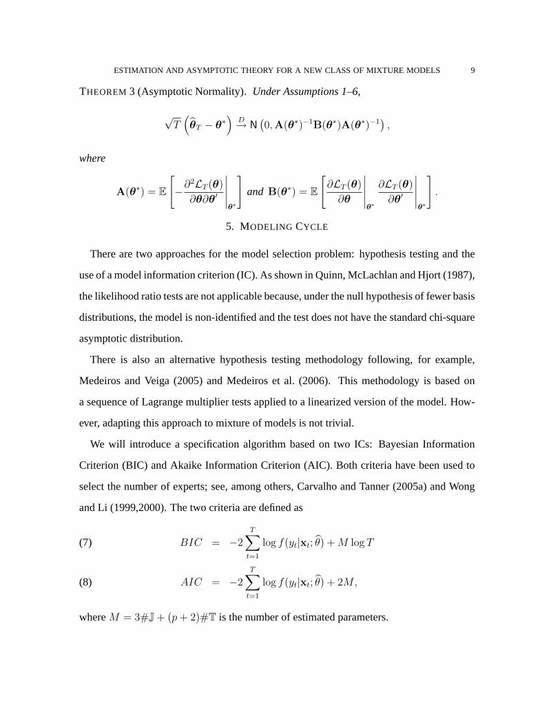
THEOREM 3 (Asymptotic Normality).Under Assumptions 1–6,

√T

(θT − θ∗

)D→ N

(0,A(θ∗)−1

B(θ∗)A(θ∗)−1),

where

A(θ∗) = E

[−∂

2LT (θ)

∂θ∂θ′

∣∣∣∣∣θ∗

]and B(θ∗) = E

[∂LT (θ)

∂θ

∣∣∣∣∣θ∗

∂LT (θ)

∂θ′

∣∣∣∣∣θ∗

].

5. MODELING CYCLE

There are two approaches for the model selection problem: hypothesis testing and the

use of a model information criterion (IC). As shown in Quinn, McLachlan and Hjort (1987),

the likelihood ratio tests are not applicable because, under the null hypothesis of fewer basis

distributions, the model is non-identified and the test doesnot have the standard chi-square

asymptotic distribution.

There is also an alternative hypothesis testing methodology following, for example,

Medeiros and Veiga (2005) and Medeiros et al. (2006). This methodology is based on

a sequence of Lagrange multiplier tests applied to a linearized version of the model. How-

ever, adapting this approach to mixture of models is not trivial.

We will introduce a specification algorithm based on two ICs: Bayesian Information

Criterion (BIC) and Akaike Information Criterion (AIC). Both criteria have been used to

select the number of experts; see, among others, Carvalho andTanner (2005a) and Wong

and Li (1999,2000). The two criteria are defined as

BIC = −2T∑

t=1

log f(yt|xt; θ) +M log T(7)

AIC = −2T∑

t=1

log f(yt|xt; θ) + 2M,(8)

whereM = 3#J + (p+ 2)#T is the number of estimated parameters.

10 ESTIMATION AND ASYMPTOTIC THEORY FOR A NEW CLASS OF MIXTURE MODELS

It is known that, for well behaved models, BIC is consistent for model selection. Fur-

thermore, when the sample size goes to the infinity, the true model will be selected because

it has the smallest BIC with probability tending to one. However, when the model is overi-

dentified, the usual regularity conditions to support this result fail, but Wood, Jiang and

Tanner (2001) present some evidence that, even when we have overidentified models, the

BIC may still be consistent for model selection.

J andT define the treeJT with #T local models and letk ∈ T be a node to be split.

When we split the nodek we have the new treeJT(k) defined byJ(k) andT(k), where

J(k) = J ∪ {k}(9)

T(k) = {2k + 1, 2k + 2} ∪ (T \ {k}) ,(10)

whereT \ {k} is the complement of{k} in T. The new parameter vectorθ(k) is defined as

(11) θ(k) =[ν ′j1, . . . ,ν ′

j#J(k)

, ψ′t1, . . . , ψ′

t#T(k)

]′,

whereji ∈ J(k) andti ∈ T(k).

The growing algorithm for the first split is the following: (1) set the number of covariates

asp and estimate a linear model with allp regressors and compute the value of the IC; (2)

for each covariatexs0 ∈ xt with s0 = 1, . . . , p, estimate the modelJT(0), where each

terminal node is a linear model with allp regressors, and compute the IC; and (3) select the

model with the smallest IC.

The growing algorithm for thek-th split is: (1) for eachk ∈ T and for eachxsi∈ xt with

si = 1, . . . , p, (a) split the nodek following (9) and (10), (b) estimate the new parameter

vectorθ(k) as in (11), and (c) compute the IC; (2) select the treeJT(k) with the smallest IC;

(3) if the smallest IC for the treeJT(k) is greater than the IC of the treeJT, then we stop

growing the tree. Case contrary, repeat the steps above settingJT = JT(k).


6. MONTE-CARLO STUDY

Consider the following models:

• Model 1: a linear AR(2) model.

yt = 1.0 + 0.5yt−1 − 0.2yt−2 + εt, εt ∼ NID(0, 1.0).

• Model 2: a Tree-MM model with two AR(4) local models,J = {0}, T = {1, 2},

andg0(·; γ0, c0) = g(yt−4; 2, 3). The local models are:

y1t = 2.0 − 0.1yt−1 + 0.7yt−2 + 0.2yt−4 + ε1t, ε1t ∼ NID(0, 1.0)

y2t = 2.0 + 0.2yt−1 − 0.6yt−2 + 0.3yt−3 − 0.3yt−4 + ε2t, ε2t ∼ NID(0, 0.6).

• Model 3: a Tree-MM model with three local AR(2) models,J = {0, 2}, T =

{1, 5, 6}, g0(·; γ0, c0) = g(yt−2; 2, 1), g2(·; γ2, c2) = g(yt−1; 2, 4), and

y1t = 0.5 − 0.4yt−1 + 0.7yt−2 + ε1t, ε1t ∼ NID(0, 1.0)

y5t = 4.0 + 0.8yt−1 − 0.5yt−2 + ε5t, ε5t ∼ NID(0, 0.6)

y6t = 8.0 − 0.9yt−1 + 0.2yt−2 + ε6t, ε6t ∼ NID(0, 1.1).

• Model 4: a Tree-MM model with four local AR(2) models,J = {0, 1, 2}, T =

{3, 4, 5, 6}, g0(·; γ0, c0) = g(yt−2; 1, 1), g1(·; γ1, c1) = g(yt−1; 3, 0), g2(·; γ2, c2) =

g(yt−1; 2, 4), and

y3t = 0.7yt−1 − 0.3yt−2 + ε3t, ε3t ∼ NID(0, 0.7)

y4t = −0.5 − 0.4yt−1 + 0.7yt−2 + ε4t, ε4t ∼ NID(0, 1.0)

y5t = 4.0 + 0.8yt−1 − 0.5yt−2 + ε5t, ε5t ∼ NID(0, 0.6)

y6t = 8.0 − 0.9yt−1 + 0.2yt−2 + ε6t, ε6t ∼ NID(0, 1.1).


Models 1–4 are used to evaluate the small sample properties of the QMLE and the mod-

eling cycle strategy. The results are presented in the following subsections.

6.1. Parameter estimation. We present the empirical results of the estimation of the pa-

rameters of Models 2–4. We report the mean, the median, the standard deviation, and the

median absolute deviation around the median (MAD) across 2000 replications. The MAD

is defined asMAD(θ) = median(∣∣∣θ − median(θ)

∣∣∣)

.

We have simulated Models 2–4 with two different sample sizes: 150 and 500 observa-

tions. Tables 1–3 show estimation results for each model. From the tables, it is clear that

the estimation turns to be rather precise, with the only exception of the slope parameterγ,

which is usually overestimated. This overestimation were noticed in Medeiros and Veiga

(2005), and it is caused by the lack of observations around the transition location.

TABLE 1. SIMULATED MODEL 2: DESCRIPTIVE STATISTICS OF THE ESTIMATES.

The table shows the mean, the standard deviation (SD), the median, and themedian absolute deviation (MAD) of the estimates of the parameters of Model 2over 2000 simulations. 150 and 500 observations are considered.

150 500Actual Mean SD Median MAD Mean SD Median MAD

γ0 2.00 5.06 1.75 4.68 0.89 5.01 1.65 4.66 0.83c0 3.00 3.01 0.23 3.02 0.15 3.00 0.22 3.00 0.15σ2

1 1.00 0.95 0.14 0.94 0.09 0.95 0.13 0.95 0.09β01 2.00 2.00 0.11 2.00 0.07 2.00 0.10 2.00 0.07β11 -0.10 -0.10 0.04 -0.10 0.03 -0.10 0.04 -0.10 0.03β21 0.70 0.70 0.04 0.70 0.02 0.70 0.04 0.70 0.02β31 0 0.00 0.05 0.00 0.03 0.00 0.04 0.00 0.03β41 0.20 0.20 0.06 0.20 0.04 0.20 0.06 0.20 0.04σ2

2 0.60 0.31 0.08 0.31 0.05 0.30 0.08 0.31 0.05β02 2.00 1.99 0.36 1.99 0.23 2.01 0.34 2.01 0.20β12 0.20 0.20 0.05 0.20 0.03 0.02 0.72 0.22 0.08β22 -0.60 -0.60 0.06 -0.60 0.04 -0.60 0.06 -0.60 0.03β32 0.30 0.03 0.05 0.30 0.03 0.03 0.04 0.30 0.03β42 -0.30 -0.30 0.06 -0.30 0.04 -0.30 0.04 -0.30 0.04





γ0 2.00 5.41 2.25 4.98 1.25 4.99 1.17 4.86 0.66c0 1.00 0.97 0.35 0.97 0.18 0.94 0.20 0.94 0.12σ2

1 1.00 0.87 0.44 0.87 0.18 0.97 0.15 0.96 0.10β01 0.50 0.63 0.98 0.51 0.19 0.51 0.15 0.40 0.09β11 -0.40 -0.39 0.27 -0.41 0.08 -0.40 0.06 -0.40 0.04β21 0.70 0.62 0.48 0.66 0.10 0.68 0.08 0.69 0.05γ2 2.00 5.47 2.48 4.89 1.36 5.21 1.64 4.85 0.88c2 4.00 3.92 0.42 3.95 0.14 3.92 0.2 3.93 0.13σ2

5 0.60 0.34 0.09 0.33 0.05 0.35 0.04 0.35 0.03β05 4.00 3.99 0.24 4.00 0.14 4.00 0.11 4.00 0.07β15 0.80 0.80 0.06 0.80 0.04 0.80 0.03 0.80 0.02β25 -0.50 -0.50 0.05 -0.50 0.04 -0.50 0.03 -0.50 0.02σ2

6 1.10 1.13 0.34 1.11 0.18 1.21 0.15 1.20 0.10β06 8.00 8.09 1.48 1.09 0.79 8.07 0.62 8.06 0.39β16 -0.90 -0.90 0.21 -0.90 0.11 -0.90 0.09 -0.90 0.05β26 0.20 0.17 0.22 0.18 0.11 0.18 0.09 0.18 0.06

6.2. Specification Algorithm. We simulate 200 replications of Models 1–4 with two sam-

ple sizes: 150 and 500 observations. Table 4 presents the number of times a model is cor-

rectly (C)/incorrectly (I) specified. We define the model to becorrectly specified if the sets

J, T andS = {s0, . . . , s#J} are equal to the true setsJ0, T0 andS0. The tree is incorrectly

specified if any of these sets are different.

The BIC has a better performance then AIC in small and large samples. As expected,

the performance of the modeling strategy improves as the sample sizes increases.

6.3. Approximation Capabilities. We illustrate the ability of the Tree-MM model to ap-

proximate unknown conditional probability density functions. We simulate two AR(1)-

GARCH(1,1) models and two NN models. We generate 2000 observations, where the first

1000 are used for estimation and the remaining 1000 for out-of sample evaluation.





γ0 1.00 3.41 1.62 3.07 0.67 3.38 1.14 3.16 0.52c0 1.00 0.98 0.42 0.94 0.19 0.96 0.23 0.94 0.12γ1 3.00 6.07 3.29 5.51 2.31 6.39 3.02 6.12 2.27c1 0.00 0.04 0.49 0.04 0.20 0.01 0.34 0.02 0.15γ2 2.00 5.44 3.04 4.69 2.02 5.13 2.86 4.43 1.91c2 4.00 3.48 0.87 3.68 0.40 3.59 0.67 3.74 0.29σ2

3 0.70 0.45 0.29 0.42 0.08 0.47 0.17 0.46 0.05β03 0.00 -0.02 0.35 -0.02 0.17 -0.02 0.17 -0.01 0.09β13 0.70 0.68 0.16 0.69 0.08 0.69 0.08 0.69 0.04β23 -0.30 -0.31 0.10 -0.31 0.05 -0.31 0.05 -0.31 0.03σ2

4 1.00 0.87 0.37 0.85 0.18 0.95 0.16 0.94 0.10β04 -0.50 -0.56 0.46 -0.57 0.28 -0.53 0.22 -0.53 0.15β14 -0.40 -0.40 0.17 -0.40 0.10 -0.40 0.08 -0.40 0.05β24 0.70 0.67 0.17 0.67 0.10 0.68 0.09 0.68 0.05σ2

5 0.60 0.33 0.14 0.31 0.06 0.34 0.05 0.34 0.03β05 4.00 4.00 0.19 4.00 0.11 4.00 0.08 4.00 0.05β15 0.80 0.80 0.05 0.80 0.03 0.80 0.02 0.80 0.02β25 -0.50 -0.50 0.05 -0.50 0.02 -0.50 0.02 -0.50 0.01σ2

6 1.10 1.14 0.67 1.04 0.31 1.28 0.37 1.23 0.18β06 8.00 7.94 2.17 8.00 1.08 7.81 1.08 7.91 0.57β16 -0.90 -0.86 0.37 -0.88 0.17 -0.84 0.18 -0.86 0.09β26 0.20 0.12 0.29 0.13 0.15 0.16 0.12 0.16 0.07

TABLE 4. SPECIFICATION ALGORITHM.

This table shows the number of cases where the each modelis correctly (C)/incorrectly (I) specified. We consider two dif-ferent samples: 150 and 500 observations. Both the AIC andBIC are used to select the structure of the models.

150 500AIC BIC AIC BIC

Model C I C I C I C I1 163 37 172 28 197 3 200 02 107 93 134 66 193 7 196 43 83 117 96 104 150 50 166 344 57 143 81 119 123 77 135 65


We use the coverage test Christoffersen (1998) over a set of percentiles to evaluate the

coverage. The test is applied to the out-of-sample period. The correlation and the mean

squared error (MSE) of the one-step-ahead predictions are also used to compare the Tree-

MM models with the true data generation process. The Christoffersen´s (1998) test consists

in two likelihood ratio (LR) tests. The first one is the LR test of unconditional coverage

and the second one the LR test of independence.

All the AR(1)-GARCH(1,1) models have the same linear part and distinct GARCH(1,1)

conditional variances. The linear model is:

yt = 0.7yt−1 + ut,

whereut = h1/2t ǫt, ǫt ∼ NID(0, 1), and

• Model 5:ht = 10−5 + 0.85ht−1 + 0.05u2t−1;

• Model 6:ht = 10−5 + 0.90ht−1 + 0.085u2t−1.

The simulated NN models are the following:

yt = 0.1 + 0.75yt−1 − 0.05yt−4 + 0.8g(0.45yt−1 − 0.89yt−4; 2.24,−0.09)

−0.7g(0.44yt−1 + 0.89yt−4; 1.12,−0.35) + ut,

whereut = h1/2t ǫt, ǫt ∼ NID(0, 1), and

• Model 7:ht = 1;

• Model 8:ht = 10−5 + 0.85ht−1 + 0.05ǫ2t−1.

We evaluate the conditional coverage over the following tail percentiles: 90%, 95%,

97.5% and 99%. Table 5 shows empirical coverage and the results of the Christoffersen´s

(1998) test.LRuc is thep-value of the unconditional coverage test andLRcc is thep-value

of the conditional coverage test. From the results, it is clear that the Tree-MM is able to

model the tail of conditional distribution.


TABLE 5. EMPIRICAL COVERAGE.

The table shows the empirical coverage and thep-value of theChristoffersen test for the estimated AR(1)-GARCH(1,1) andNN-GARCH(1,1) models.LRuc andLRcc are thep-values ofthe unconditional conditional coverage tests, respectively.

Empirical Coverage90.0 95.0 97.5 99.0

Est. Percentile 90.39 95.60 97.60 99.20Model 5 LRuc 0.695 0.389 1.000 0.534

LRcc 0.223 0.184 0.596 0.202Est. Percentile 90.76 95.51 97.10 99.00

Model 6 LRuc 0.457 0.918 0.215 0.273LRcc 0.542 0.228 0.118 0.273

Est. Percentile 89.30 95.00 97.40 99.20Model 7 LRuc 0.3344 .6878 1.000 .5297

LRcc 0.2939 .6664 .3583 .2349Est. Percentile 90.60 95.40 97.10 99.00

Model 8 LRuc 0.5352 0.5735 0.4385 1.000LRcc 0.6199 0.6018 0.5317 0.000

Table 6 compares the out-of-sample performance of the estimated Tree-MM model with

the true NN specification. The correlation row shows the average correlation between

the estimates, MSENN and MSETree-MM are the average out-of-sample MSE for the NN and

Tree-MM models, respectively. From the results in the tables we can see that the correlation

between the estimates are high and the MSEs are very close forboth models, showing the

approximation capabilities of the Tree-MM models.

TABLE 6. FORECASTINGPERFORMANCERESULTS.

The table shows the forecasting results and the corre-lation between the true data generating process and theestimated Tree-MM model.

Model Correlation MSENN MSETree-MM

Model 7 0.88 0.0223 0.0242Model 8 0.74 2.25 × 10−3 2.81 × 10−3


7. EXAMPLES

7.1. Example 1: Canadian Lynx. The first set analyzed is the 10-based logarithm of the

annual record of the numbers of Canadian Lynx trapped in the Mackenzie River district

of north-west Canada for the period 1821–1934 (114 observations). For further details

and background history, see Tong (1990).We report only the results for in-sample fitting

because the number of observations is rather small and most of the previous studies in

literature have only considered the in-sample analysis. Itis commonly accepted that the

data are cyclical, with a period of 9-10 years and multimodality.

The variables are selected following the methodology of Rech, Terasvirta and Tschernig

(2001). The final model using either AIC or BIC is a 1-split tree, where the transition

variable is theyt−2 and

g0(·) = g(yt−2; 9.9826, 2, 3.2655),

y1t = 0.5465 + 1.319yt−1 − 0.4655yt−2 + ε1t ε1t ∼ N(0, 0.0325),

y2t = 0.9892 + 1.5173yt−1 − 0.8832yt−2 + ε2t ε2t ∼ N(0, 0.0493).

We compare the Tree-MM model with the following alternatives: an AR(2) model; the

SETAR model of Tong (1990); the MAR model of Wong and Li (2000); and the GMAR

model of Wong and Li (1999). The models MAR and GMAR have a mixture of Gaussian

models as the conditional density and the others have a Gaussian conditional density. The

final Tree-MM model has the same number of regimes and the sametransition variable as

the models SETAR and GMAR.

All the models have similar empirical coverage. However, itterms of the conditional

mean fit, the Tree-MM model attains the lowest mean absolute error (MAE).

7.2. Example 2: Brazilian Financial Dataset. In this section we apply the Tree-MM

model to automatic trading using data from the Brazilian stock exchange. We compare the


TABLE 7. EXAMPLE 1: EMPIRICAL COVERAGE.

The table shows the empirical coverage as well as the mean absoluteerror (MAE) for a set of different models.

Empirical CoverageModel 50 60 70 80 90 95 MAEAR(2) 50.00 58.93 68.75 75.89 88.61 92.86 1.99SETAR 44.86 56.07 69.16 81.31 90.65 95.33 2.27MAR 52.68 63.39 70.54 82.14 88.39 96.43 2.36

GMAR 47.32 58.93 68.75 82.14 92.86 93.75 2.25Tree-MM 48.21 57.14 67.86 79.46 89.29 96.43 1.89

results with an NN model estimated with Bayesian regularization (MacKay 1992), with the

ARMA model, and the naıve method (the forecast for any period equals the previous pe-

riod’s actual value). We choose an asset which tracks the BOVESPA Index (IBOVESPA).

IBOVESPA is an index of the 50 most liquid stocks traded at the Sao Paulo Stock Exchange.

The selected asset is the Petrobras PN (PETR4) (Brazilian Oil Company). The observa-

tions cover the period from 01/20/1999 to 12/30/2004 (1476 observations). The sample is

divided into two groups. The first one consists of 1227 observations (from 01/20/1999 to

12/30/2003) and is used to estimate the model. The second group consists of 249 observa-

tions (from 02/02/2004 to 12/30/2004) and it is used for out-of-sample evaluation.

The set of possible covariates is composed by the first 10 lagsof the log-return of the

asset, the first 10 lags of the volatility, the first 10 lags of the traded volume between 2

days, the first difference of the 10- and 20-days moving averages of the return (MA10

and MA20, respectively), and the first difference of the following 10 exogenous variables:

IBOVESPA, S&P 500 Index (S&P), US Dollar exchange rate (DOL),10-year Treasury bill

(T10), C-Bond (C-BOND), the spread between C-Bond and T10 (SOT), Oil price (OIL),

Swap 360 (SW360), a set of commodities (CRY) and the DevelopingCountries Stock Index

(BINDEX).

The statistical measures used to evaluate the model are the mean absolute error (MAE),

the root mean square error (RMSE), and the correct direction of change (CDC). The


financial measures are the average return (R), the annual return (RA), the accumulate return

(RC), the annual volatility (σA), the Sharpe index (SR), the number of trades (#T ), and the

percentage of winning trades (WT ). Furthermore, we present the coverage of the model

and the statistics of the coverage for the NN and Tree-MM models. The trading strategy

is the following. We sell the stock every time the forecastedreturn is negative and we buy

when the forecasted return is positive. Table 8 shows the results.

We first select the set of regressors using the procedure proposed by Rech et al. (2001).

The final Tree-MM model is given by:

g0(·) = g(vt−1; 5.2572, 2, 0.0318),

y1t = −7.9906 × 10−4 − 0.0542yt−1 + 0.0775vt−1 + 5.0897 × 10−4qt−1

−3.6653 × 10−6MA10 + 0.0180CRY + ε1t ε1t ∼ N(0, 1.9374 × 10−4),

y2t = −6.956 × 10−3 + 0.3382yt−1 + 0.1673vt−1 + 1.5762 × 10−3qt−1

−1.6057 × 10−5MA10 + 0.0167CRY + ε2t ε2t ∼ N(0, 6.5584 × 10−4).

The estimated NN model has two hidden units and uses the wholeset of variables. The

Tree-MM model, the NN model and the linear model have similarperformance accordind

to the statistical measures. However, the financial measures indicate that the Tree-MM

model has the best performance among the competing models.

8. CONCLUSIONS

In this paper we proposed a new mixture of models based on smooth transition regression

trees. A quasi-maximum likelihood estimator was developedand its asymptotic properties

were derived under mild regularity conditions. A model building strategy was also consid-

ered. Monte Carlo simulations gave strong support for the theory developed here, even in

small samples. Two applications with real data were used to illustrate the model.


TABLE 8. STATISTICAL AND FINANCIAL RESULTS

This table shows the mean absolute error (MAE), theroot mean square error (RMSE), the correct directionof change (CDC), and the averageR), the annual (RA),and the accumulated (RC) returns, respectively. The ta-ble also shows the annual volatility (σA), the Sharpe in-dex (SR), the number of trades (#T ), and the percent-age of winning trades (WT ).

ARMA Naıve NN TREE-MMMAE 0.012 0.016 0.012 0.012RMSE 0.017 0.022 0.017 0.017CDC 60.48 58.07 65.73 62.50

R 0.68 0.50 1.65 1.45RA 41.64 26.38 60.47 61.69RC 40.98 25.96 59.51 60.71σA 24.45 22.59 18.47 18.31SR 1.70 1.17 3.27 3.37#T 60 52 36 42WT 55.00 % 46.67 % 75.00 % 76.19%

APPENDIX A. I DENTIFIABILITY

Let JT be a tree with setsJ, T andS, whereS is the set of indexessj, ∀j ∈ J and

parameter vectorθ. We define a subtreeJTk as the tree beginning at nodek, with the sets

Jk ⊆ J, Tk ⊆ T andSk ⊆ S, wherei ∈ JTk ⇔ k ∈ Ji ∪ {i} and parameter vectorθk. For

example, assume the treeJT = {0, 1, 2, 3, 4, 5, 6, 11, 12} thenJT2 = {2, 5, 6, 11, 12}.

ASSUMPTION7. Letfk(yt|xt;θk) be the conditional p.d.f. of the subtreeJTk. Then∀k ∈

J, f2k+1(yt|xt;θ2k+1) 6= f2k+2(yt|xt;θ2k+2).

This assumption guarantees that our tree is irreducible in the sense that any split cannot

be changed by a subtree or by a local model.


ASSUMPTION8. We assume that for any treeJT and all sub-treesJTk: (1) γj > 0,∀j ∈ J;

(2) ∀j ∈ J2k+1, if sj = sk thencj < ck; (3) ∀j ∈ J2k+2, if sj = sk thencj ≥ ck.

These assumptions together ensure that the setsJ, T andS uniquely specify any tree.

LEMMA 1. Under Assumptions (7) and (8), a treeJT is uniquely specified and the param-

eter vectorθ has a unique representation.

PROOF. Suppose that for any nodek ∈ J, f2k+1(yt|xt;θ2k+1) = f2k+2(yt|xt;θ2k+2) such

thatfk = gk(·)f2k+1 + (1 − gk(·))f2k+2 = f2k+1 = f2k+2. Hence, we can change the node

k by the node2k + 1 or 2k + 2. If f2k+1(·) 6= f2k+2(·), ∀k ∈ J, then the tree cannot be

reduced, so it is irreducible.

Now, suppose there is an irreducible treeJT. On the first split ats0, c0 can assume any

value inR. Now consider the sub-treesJT1 andJT

2. Following the condition (8), on the

next split atsk = s0, k ∈ J1, ck can assume any value in(−∞, c0) and on the next split

at sl = s0, l ∈ J2, cl can assume any value in[c0,∞). So, the values ofck andcl cannot

be interchanged. Repeating this argument for all splits, andconsidering that the transition

has the same shape (which is guaranteed by the constraint over theγs), we show that any

irreducible tree under Assumption (8) is uniquely specified.

Q.E.D.

The next theorem gives the conditions under which the Tree-MM model is identifiable.

THEOREM 4. Under Assumptions (7) and (8), and assuming thatπ(yt|xt;ψ) is uniquely

identified by a parameter vectorψ, model (2) is identifiable, in the sense that, for a sample

{yt;xt}Tt=1, and forθ1, θ2 ∈ Θ

T∏

t=1

f(yt|xt;θ1) =T∏

t=1

f(yt|xt;θ2) , a.s.


is equivalent toθ1 = θ2.

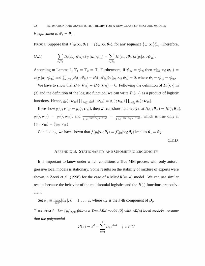
PROOF. Suppose thatf(yt|xt;θ1) = f(yt|xt;θ2), for any sequence{yt;xt}Tt=1. Therefore,

(A.1)∑

i∈T1

Bi(xsi;θ1i)π(yt|xt;ψ1i) =

∑

i∈T2

Bi(xsi;θ2i)π(yt|xt;ψ2i).

According to Lemma 1,T1 = T2 = T. Furthermore, ifψ1i = ψ2i thenπ(yt|xt;ψ1i) =

π(yt|xt;ψ2i) and∑

i∈T(Bi(·;θ1i) −Bi(·;θ2i))π(yt|xt;ψi) = 0, whereψi = ψ1i = ψ2i.

We have to show thatBi(·;θ1i) − Bi(·;θ2i) = 0. Following the definition ofBi(·; ·) in

(3) and the definition of the logistic function, we can writeBi(·; ·) as a product of logistic

functions. Hence,g0(·;ν10)∏

k∈Jigk(·;ν1k) = g0(·;ν20)

∏k∈Ji

gk(·;ν2k).

If we showg0(·;ν10) = g0(·;ν20), then we can show iteratively thatBi(·;θ1i) = Bi(·;θ2i),

g0(·;ν10) = g0(·;ν20), and 1

1+e−γ10(xs0,t−c10) = 1

1+e−γ20(xs0,t−c20) , which is true only if

(γ10, c10) = (γ20, c20).

Concluding, we have shown thatf(yt|xt;θ1) = f(yt|xt;θ2) impliesθ1 = θ2.

Q.E.D.

APPENDIX B. STATIONARITY AND GEOMETRIC ERGODICITY

It is important to know under which conditions a Tree-MM process with only autore-

gressive local models is stationary. Some results on the stability of mixture of experts were

shown in Zeevi et al. (1998) for the case of a MixAR(m; d) model. We can use similar

results because the behavior of the multinomial logistics and theB(·) functions are equiv-

alent.

Setαk ≡ maxi∈T

|βik|, k = 1, . . . , p, whereβik is thek-th component ofβi.

THEOREM 5. Let {yt}t≥0 follow a Tree-MM model (2) with AR(p) local models. Assume

that the polynomial

P(z) = zd −p∑

k=1

αkzd−k ; z ∈ C


has all its zeros in the open unit disk,z < 1. Then the vector processyt has a unique

stationary probability measure, and is geometrically ergodic.

PROOF. To use the results of Zeevi et al. (1998), we need to show somesimilarities between

the multinomial logit and theB(·) functions. SetB(1) as the left most expert of the tree and

B(J) as the right most expert.B(1) is a product of1 − g(·) functions andB(J) is a product

of g(·) functions. AnyB(j) for j = 2, . . . , J − 1 has at least one termg(·) and one term

1− g(·). We can show the equivalence of the proofs if we satisfy the following conditions:

(i) B(1) → 1 for ys(1) → −∞; (ii) B(1) → 0 for xs(1) → ∞; (iii) B(J) → 1 for xs(J) → ∞;

(iv) B(J) → 0 for xs(J) → −∞; and (v)B(j) → 0 for xs(j) → ±∞.

We know thatg(xt,νk) → 1 for xsk→ ∞ andg(xt,νk) → 0 for xsk

→ −∞. Thus,

[1 − g(xt,νk)] → 0 for xsk→ ∞, [1 − g(xt, νk)] → 1 for xsk

→ −∞, and

limx

s(1)→−∞

B(1)(·) = limx

s(1)→−∞

∏[1 − g(·)] =

∏lim

xs(1)

→−∞[1 − g(·)] = 1,

such that Condition (i) holds. Conditions (ii)–(v) can be verified using the same steps.

Q.E.D.

APPENDIX C. PROOFS OFTHEOREMS

We follow White (1992), to prove the existence, consistency and asymptotic normality

of the QMLE. Besides, we define some notation to make the proofsclearer.

Define ft ≡ f(yt|xt; θ), f ∗t ≡ f(yt|xt;θ∗), πit ≡ π(yt|xt;ψi), π

∗it ≡ π(yt|xt;ψ∗

i ),

Bit ≡ Bi(xt;θi), andB∗it ≡ Bi(xt;θ

∗i ). Furthermore, define recursivelyfk,t = (1 −

g(xsk;νk))f2k+1,t + g(xsk

;νk)f2k+2,t, for all k in J, andfk,t = πkt, for all k in T.

C.1. Proof of Theorem 1. We need to satisfy Assumptions 2.1, 2.3 and 2.4 of Theorem

2.13 in White (1992) and show that|LT (θ)| < ∞ with θ∗ being the unique maximum of

LT (θ). Assumption 2.1 is satisfied by Assumption 1, and Assumption2.3 is satisfied by


Assumption 2 and Lemma 2. Assumption 2.4 and|L(θ)| < ∞ are satisfied by Lemma 2.

So we need to show thatLT (θ) has a unique maximum atθ∗.

First, we write the maximization problem as follows:

maxθ∈Θ

[LT (θ) − LT (θ∗)] = maxθ∈Θ

E

[log

f ∗t

ft− ftf ∗t

− 1

].

Furthermore, for anyx > 0,m(x) = x− log(x) ≤ 0, then

E

[log

f ∗t

ft− ftf ∗t

]≤ 0.

Given thatm(x) archives its maximum atx = 1, E[m(x)] ≤ E[m(1)] with equality

holding almost surely only iff ∗t = ft with probability one. By the mean value theorem, it

is equivalent to show that

(C.2) (θ − θ∗)′∂ log ft∂θ

= 0

almost surely. A straightforward application of Lemma 3 shows that it happens if, and only

if, θ = θ∗ with probability one, which completes the proof.

Q.E.D.

C.2. Proof of Theorem 2. We must satisfy Assumptions 2.1, 2.3, 2.4, 3.1, and 3.2’ of

Theorem 3.5 in White (1992). Assumptions 2.1, 2.3, 2.4 and 3.2’ are satisfied by Assump-

tions 1–3. Assumption 3.1 states that: (a)EG(log ft) <∞,∀t; (b) EG(log ft) is continuous

in Θ; and (c){log ft} obeys the uniform law of large numbers (ULLN).

It is clear thatEG(log ft) ≤ log EG(ft) ≤ log EG(suptft). But sup

tft = ∆ < ∞, then

log

[EG(sup

tft)

]= log ∆ < ∞ and (a) is satisfied. In addition,log(·), Gt and ft are

continuous, measurable, and integrable functions, soht = Gt log ft is also continuous,

measurable, and integrable. Then,∫htdy is continuous and (b) is satisfied. Finally, (c) is

satisfied by Lemma 8.


Q.E.D.

C.3. Proof of Theorem 3. We must satisfy Assumptions 2.1, 2.3, 3.1, 3.2’, 3.6, 3.7(a), 3.8,

3.9 and 6.1 in White (1992). Assumptions 2.1, 2.3, 3.1, 3.2’ are satisfied by Assumptions

1–6 (see proof of Theorem 2). Assumption 3.6 is satisfied by Lemma 2, Assumption 3.7(a)

is satisfied by Lemma 5, Assumption 3.8 by Lemmas 6 and 8, Assumption 3.9 by Lemma

7, and Assumption 6.1 is shown here.

Assumption 6.1 requires that{T−1/2∂θft|θ∗

}obeys a central limit theorem with covari-

ance matrixB(θ∗), whereB(θ∗) isO(1) and uniformly positive definite. We must show the

following to satisfy Assumption 6.1: (a)T−1∑T

t=1 ∂θft|θ∗∂θ′ft|θ∗a.s.→ E(∂θft|θ∗∂θ′ft|θ∗);

(b) the sequence is strictly stationary.

Condition (a) is readily verified by Lemmas 8 and 5. Condition (b) is satisfied by As-

sumptions 4 and 6. Hence, satisfying these assumptions, theresult follows.

Q.E.D.

APPENDIX D. LEMMAS

LEMMA 2. Under Assumptions (2)–(3),f(yt|xt;θ) is a measurable, limited, positive and

continuously differentiable function ofY t = [yt,xt]′ onΘ.

PROOF. Trivially, π(yt|xt;ψi) andg(xsjt;νj) are continuous, mensurable, finite, positive

and differentiable functions ofY t. The functionf(yt|xt;θ) is a sequence of sums and

products of these functions. As a result,f(yt|xt;θ) is a continuous, mensurable, finite,

positive and differentiable function ofY t.

Q.E.D.

LEMMA 3. Letd be a constant vector with the same dimension ofθ. Then, it follows that

d′

(∂ log ft∂θ

)= 0 a.s.


if, and only if,d = 0.

PROOF. First, writed′

(∂ log ft∂θ

)= d′ 1

ft

∂ft∂θ

= 0. From Lemma 2, we know thatft > 0.

Hence,

d′∂πit∂ψi

= 0 and [f2k+1,tgkt − f2k+2,t(1 − gkt)]d′∂[−γk(yt − ck)]

∂νk= 0,

which are both functions ofyt. By the non-degeneracy condition, and supposing thatyt is

not null for all t, d′ ∂ft

∂θ= 0 if, and only if,d = 0.

Q.E.D.

LEMMA 4. Under Assumptions 2, 5 and 6,E(log ft) <∞.

PROOF. Write log ft = log∑

i∈TBitπit < log

∑i∈T

πit < log #T + log supi∈T πit. Let

πIt = π(yt|xt;x′tβI , σ

2I ) = supi∈T πit. Then,log πIt = −1

2log 2πσ2

I − 12σ2

I

(x′tβI − yt)

2.

Under Assumptions 2 and 5,E [log πIt] = −12log 2πσ2

I − 12σ2

I

E [(x′tβI − yt)

2] <∞.

Q.E.D.

LEMMA 5. Under Assumptions 2, 4, 5 and 6,

E

(∂ log ft∂θ

)<∞ and E

(∂ log ft∂θ

∂ log ft∂θ′

)<∞.

PROOF. Let ∂θ ≡ ∂∂θ

. It is clear that

(D.3) ∂θ log ft =1

ft∂θft =

1

ft

∑

i∈T

πit∂θBit +Bit∂θπit ≤ ∆π,f

∑

i∈T

∂θBit + ∆B

∑

i∈T

∂θπit,

where∆π,f = supi(f−1t πit) < ∞ and∆B = supi f

−1t < ∞. Set∂ψi

≡ ∂/∂ψi, ∂νj≡

∂/∂νj, and∆π = supi πit. Hence,

∂ψiπit = πit∂ψi

log πit ≤ ∆π∂ψilog πit,(D.4)

∂νjBit = Bit(−gjt)(1 − gjt)∂νj

[−γj(xsj− cj)] ≤

∣∣∂νj[−γj(xsj

− cj)]∣∣ .(D.5)


Asψi = [β0i, . . . , βpi, σ2i ]

′, the right size of (D.4) can be written as

∆π∂βkilog πit = −∆π

xkt(x′tβ − yt)

σ2i

,(D.6)

∆π∂σ2ilog πit = ∆π

(− 1

2σ2i

+(x′tβ − yt)

2

2σ4i

),(D.7)

wherexkt is thek-th element of the vectorxt.

Using the same argument, we can write the right side of equation (D.5) as

∣∣∂γj[−γj(xsj

− cj)]∣∣ =

∣∣−(xsj− cj)

∣∣ ,(D.8)

∣∣∂cj [−γj(xsj− cj)]

∣∣ = |γj| .(D.9)

It is readily verified that, under Assumptions 2, 4 and 5, the expected values of (D.6)

– (D.9) are finite. Furthermore, under Assumption 6, the expected value of any product

between these equations is also finite.

Q.E.D.

LEMMA 6. Under Assumptions 2, 4, 5 and 6,E(∂2 log ft/∂θ∂θ′) <∞.

PROOF. Set∂θθ′ ≡ ∂∂θ∂θ′

. It is clear that

(D.10) ∂θθ′ log ft = −∂θ log ft∂θ′ log ft + f−1t ∂θθ′ft.

Using the product law of differentiation, we can write∂θθ′ft as a sum of products of

∂θBit and∂θπit with ∂θθ′Bit and∂θθ′ log πit. Using the results of Lemma 5, the expected

value of the product of any two of these derivatives is finite.Therefore, we must show

that E[∂θθ′Bit] < ∞ andE[∂θθ′ log πit] < ∞. Considering thatψi andψj do not have

elements in common, and thatBit depends only on the vectorsνj, j ∈ Ji, we can write

these derivatives in terms of∂ψiψ′

iand∂νjν

′

k. Butψi = [β0i, . . . , βpi, σ

2i ]

′ andνj = [γj, cj]′.


Then,

∂βliβkilogπit = −σ−2

i xktxlt,(D.11)

∂βliσ2ilogπit = σ−4

i xlt(x′tβ − yt),(D.12)

∂σ2i σ

2ilogπit = (2σ4

i )−1σ−8

i (x′tβ − yt)

2,(D.13)∣∣∣∂νkν

′

jBit

∣∣∣ <∣∣∣∂νk

[−γk(xsk− ck)]∂ν′j [−γj(xsj

− cj)]∣∣∣ .(D.14)

Under Assumptions 2, 4 and 5, the expected values of (D.11)–(D.14) are finite.

Q.E.D.

LEMMA 7. Under Assumptions 2, 4, 5 and 6,E(∂2 log ft/∂θ∂θ′|θ∗) is negative definite.

PROOF. If E(∂2 log ft/∂θ∂θ′|θ∗) is negative definite, thenlog ft has a maximum inΘ. We

know by Lemma 3 thatlog ft has only one maximum or minimum inΘ; thus we only have

to show thatft must have a maximum.

Trivially, the Gaussian functionsπit have a maximum. If we multiply by a constant or

monotone functions or add functions with a maximum, the function still has a maximum.

The logistic function is a monotone function (in relation toits parameters and the variable).

Hence,Bitπit has a maximum andft has a maximum, andE(∂2 log ft/∂θ∂θ′|θ∗) is negative

definite.

Q.E.D.

LEMMA 8. Under Assumptions 2, 4, 5 and 6, it follows that: (a)T−1∑T

t=1 fta.s.→ E(ft);

(b)T−1∑T

t=1 ∂θfta.s.→ E(∂θft); and (c)T−1

∑Tt=1 ∂θθ′ft

a.s.→ E(∂θθ′ft).

PROOF. First we must show thatT−1∑T

t=1 yta.s.→ E(yt). Onceyt is a mixing process, we

just need to show that (i)E(T−1

∑Tt=1 yt

)= E(yt) and (ii)V

(T−1

∑Tt=1 yt

)<∞. As yt

is stationary, (i) is trivially satisfied and as∑

E(ytyt−k) < ∆ <∞, (ii) is satisfied.


Lemma 2 ensures thatft, ∂θft and∂θθ′ft are continuous functions ofyt givenθ. Besides,

Lemmas 4, 5 and 6 guarantee that the expected value is also finite. Once the functions are

continuous and the expected value is finite, we can extend theresults ofyt for ft, ∂θft and

∂θθ′ft, thereby completing the proof.

Q.E.D.

REFERENCES

Andersen, T., Bollerslev, T. and Diebold, F.: 2006, Parametric and nonparametric measurement of volatility,

in G. Elliott, C. Granger and A. Timmermann (eds),Handbook of Financial Econometrics, North-

Holland, Amsterdam.

Bollerslev, T.: 1986, Generalized autoregressive conditional heteroskedasticity,Journal of Econometrics

21, 307–328.

Carvalho, A. and Skoulakis, G.: 2004, Ergodicity and existence of moments for local mixture of linear

autoregressions,Technical report, Northwestern University.

Carvalho, A. and Tanner, M.: 2005a, Mixture-of-experts of autoregressive time series: asymptotic normality

and model specification,IEEE Transactions on Neural Networks16, 39–56.

Carvalho, A. and Tanner, M.: 2005b, Modeling nonlinear timeseries with mixture-of-experts of generalized

linear models,The Canadian Journal of Statistics33, 1–17.

Chan, K. S. and Tong, H.: 1986, On estimating thresholds in autoregressive models,Journal of Time Series

Analysis7, 179–190.

Chen, X. and Shen, X.: 1998, Sieve Extremum Estimates for Weakly Dependent Data,Econometrica66, 289–

314.

Chen, X. and White, H.: 1998, Improved Rates and Asymptotic Normality for Nonparametric Neural Net-

work Estimators,IEEE Transactions on Information Theory18, 17–39.

Christoffersen, P. F.: 1998, Evaluating interval forecasts, International Economic Review39, 841–862.

da Rosa, J. C., Veiga, A. and Medeiros, M. C.: 2008, Tree-structured smooth transition regression models,

Computational Statistics and Data Analysis52, 2469–2488.

Dempster, A. P., Laird, N. M. and Rubin, D. B.: 1977, Maximum likelihood from incomplete data via the

EM algorithm,Journal of the Royal Statistical Society, Series B39, 1–38.


Engle, R. F.: 1982, Autoregressive conditional heteroskedasticity with estimates of the variance of United

Kingdom inflation,Econometrica50, 987–1007.

Fan, J. and Yao, Q.: 2003,Nonlinear Time Series: Nonparametric and Parametric Methods, Springer-Verlag,

New York, NY.

Gallant, A. R. and White, H.: 1992, On learning the derivatives of an unknown mapping with multilayer

feedforward networks,Neural Networks5, 129–138.

Granger, C. W. J. and Terasvirta, T.: 1993,Modelling Nonlinear Economic Relationships, Oxford University

Press, Oxford.

Hornik, K., Stinchombe, M. and White, H.: 1990, Universal approximation of an unknown mapping and its

derivatives using multi-layer feedforward networks,Neural Networks3, 551–560.

Hardle, W.: 1990,Applied Nonparametric Regression, Cambridge University Press, Cambridge.

Hardle, W., Lutkepohl, H. and Chen, R.: 1997, A review of nonparametric time series analysis,International

Statistical Review65, 49–72.

Huerta, G., Jiang, W. and Tanner, M.: 2001, Mixtures of time series models,Journal of Computational and

Graphical Statistics10, 82–89.

Huerta, G., Jiang, W. and Tanner, M.: 2003, Time series modeling via hierachical mixtures,Statistica Sinica

13, 1097–1118.

Jacobs, R. A., Jordan, M. I., Nowlan, S. J. and Hinton, G. E.: 1991, Adaptive mixtures of local experts,

Neural Computation3, 79–87.

Jiang, W. and Tanner, M.: 1999, On the identifiability of mixtures-of-experts,Neural Networks12, 1253–

1258.

Jordan, M. I. and Jacobs, R. A.: 1994, Hierarchical mixturesof experts and the EM algorithm,Neural

Computation6, 181–214.

Kuan, C. M. and White, H.: 1994, Artificial neural networks: Aneconometric perspective,Econometric

Reviews13, 1–91.

Le, N., Martin, R. and Raftery, A.: 1996, Modeling flat streches, bursts, and outliers in time series using

mixture transition distribution models,Journal of the American Statistical Association91, 1504–1515.

Luukkonen, R., Saikkonen, P. and Terasvirta, T.: 1988, Testing linearity against smooth transition autoregres-

sive models,Biometrika75, 491–499.

MacKay, D. J. C.: 1992, Bayesian interpolation,Neural Computation4, 415–447.


McAleer, M.: 2005, Automated inference and learning in modeling financial volatility,Econometric Theory

21, 232–261.

Medeiros, M., Terasvirta, T. and Rech, G.: 2006, Building neural network models for time series: A statistical

approach,Journal of Forecasting25, 49–75.

Medeiros, M. and Veiga, A.: 2005, Flexible coeficient smoothtransition time series model,IEEE Transac-

tions on Neural Networks16, 97–113.

Nowlan, S. J.: 1990, Maximum likelihood competitive learning,Advances in Neural Information Processing

Systems, Vol. 2, Morgan Kaufmann, pp. 574–582.

Poon, S. and Granger, C.: 2003, Forecasting volatility in financial markets,Journal of Economic Literature

41, 478–539.

Quinn, B., McLachlan, G. and Hjort, L.: 1987, A note on the Aitkin-Rubin approach to hypothesis testing in

mixture models,Journal of the Royal Statistal Society, Series B49, 311–314.

Rech, G., Terasvirta, T. and Tschernig, R.: 2001, A simple variable selection technique for nonlinear models,

Communications in Statistics, Theory and Methods30, 1227–1241.

Taylor, S.: 1986,Modelling Financial Time Series, Wiley, Chichester.

Terasvirta, T.: 1994, Specification, estimation, and evaluation of smooth transition autoregressive models,

Journal of the American Statistical Association89, 208–218.

Tong, H.: 1978, On a threshold model,in C. H. Chen (ed.),Pattern Recognition and Signal Processing,

Sijthoff and Noordhoff, Amsterdam.

Tong, H.: 1990,Non-linear Time Series: A Dynamical Systems Approach, Vol. 6 of Oxford Statistical Science

Series, Oxford University Press, Oxford.

Tong, H. and Lim, K.: 1980, Threshold autoregression, limitcycles and cyclical data (with discussion),

Journal of the Royal Statistical Society, Series B42, 245–292.

Trapletti, A., Leisch, F. and Hornik, K.: 2000, Stationary and integrated autoregressive neural network pro-

cesses,Neural Computation12, 2427–2450.

van Dijk, D., Terasvirta, T. and Franses, P. H.: 2002, Smooth transition autoregressive models - a survey of

recent developments,Econometric Reviews21, 1–47.

Weigend, A. S., Mangeas, M. and Srivastava, A. N.: 1995, Nonlinear gated experts for time series: Discov-

ering regimes and avoiding overfitting,International Journal of Neural Systems6, 373–399.


White, H.: 1992,Estimation, Inference and Specification Analysis, Cambridge University Press, New York,

NY.

Wong, C. S. and Li, W. K.: 1999, On a generalized mixture autoregressive model,Research Report 242,

Department of Statistics and Actuarial Science, University of Hong Kong.

Wong, C. S. and Li, W. K.: 2000, On a mixture autoregressive model,Journal of the Royal Statistical Society,

Series B62, 91–115.

Wong, C. S. and Li, W. K.: 2001, On a mixture autoregressive conditional heterocedastic model,Journal of

the American Statistical Association96, 982–995.

Wood, S., Jiang, W. and Tanner, M.: 2001, Bayesian mixture ofsplines for spatially adaptative nonparametric

regression,Biometrika89, 513–528.

Zeevi, A., Meir, R. and Adler, R.: 1998, Non-linear models for time series using mixtures of autoregressive

models,Technical report, Technion.

Departamento de Economia PUC-Rio

Pontifícia Universidade Católica do Rio de Janeiro Rua Marques de Sâo Vicente 225 - Rio de Janeiro 22453-900, RJ

Tel.(21) 35271078 Fax (21) 35271084 www.econ.puc-rio.br [email protected]

no. 538 estimation and asymptotic theory for a new class ... · alvaro veiga marcelo c. medeiros...

Documents