Industriens Utredningsinstitut THE INDUSTRIAL INSTITUTE FOR ECONOMIC AND SOCIAL RESEARCH

Postadress

Bpx 5501 114 85 Stockholm

A list of Working Papers on the last pages

No. 446, 199':)

CAPITAL GAINS TAXATlON AND RESIDENTIAL MOBILITY IN SWEDEN

Gatuadress

Industrihuset Storgatan 19

by

Per Lundborg and Per Skedinger

Telefon

08·7838000 Telefax

08-6617969

November 1995

Bankgiro

446-9995 Postgiro

191592·5

November 1995

Capital Gains Taxation and Residential Mobility in Sweden*

by

Per Lundborg

and

Per Skedinger

The Industriai Institute for Economic and Social Research, Stockholm

JEL-classification: H2, R2 . Key words: Capital gains taxes, residentiai mobility .

ABSTRACT Theoretical studies have shown that capital gains taxes in the housing market may create lock-in effects but so far no empirical evidence has been presented regarding the size of these effects. For a panel of Swedish house owners in 1984-1990, we show that lock-in effects only appear for households with incom~ reductions; the size of these lock-in effects crucially depends on the magnitude of the income loss. The theoretical model and features of the Swedish tax system imply that lock-in effects depend on the degree of mismatch in the current residence and whether the households buy up or buy down.

*We are grateful to Torsten Dahlquist and Jörgen Nilsson for data assistance and to Peter Englund and Ulf Jakobsson for comments on early versions. We gratefully acknowledge fmancial support from the Swedish Council for Building Research and the Committee for the Evaluation of the Tax Reform. The paper was presented at the Tenth Annual Congress of the European Economic Association in Prague, September 1 to 4.

Correspondence: Professor Per Lundborg, the Industrial Institute for Economic and Social Research, Box 5501, S-114 85 Stockholm, Sweden. Telephone: 08-7838390; Fax: 08-661 7969; E-mail: perl@iuLse.

1

Owner-occupier housing markets are characterized by high transaction costs. There are not

only transportation costs but also various fees and taxes to be paid when houses are bought

and sold. Moreover , credit and information costs are particularly important in this market.

The idea that transaction costs are important receives support in several econometric

studies, showing that changes in housing consumption are slow in response to changes in

desired consumption.

Capital gains taxes (CGT) are widely applied in OECD countries and represent

transaction costs Of special policy interest. 1 In Sweden the CGT rules have been changed

several times, most recently in connection with the 1991 tax reform. Theoretical studies

show that CGT may reduce residential mobility , but, to the best of our knowledge, no

empirical evidence on the size of the lock-in effects has been provided. 2

The present study is an attempt at fIlling this gap. We fIrst present a theory of

residential mismatching. For a large panel of Swedish households in the Level of Living

Surveys 1981-1991 (Eriksson and Åberg (1987», we then compute the expected tax

payments associated with changing residence. Finally, we estimate the lock-in effects of

CGT.

The computations are based on the tax rules and information on the assessed tax

value (taxeringsvärdet) of the houses. Historically, the tax rules depend on whether the

households have bought up (a more expensive house) or bought down (a less expensive

one). Those buying down have been taxed more severely than those buying up. With our

data we can determine, at least roughly, how much COT the household should pay when

buying up and when buying down. Since little is known about the size of these tax

payments, a mere descriptive analysis of such data provides valuable information.

We argue that CGT, and for that matter any other transaction cost, will hamper

l See OECD (1988a, 1988b).

2See Englund (1985, 1986) and Lundborg and Skedinger (1995) for theoretical snuiies on the effects of CGT and e.g. Edin and Englund (1991), Börsch-Supan (1990) or Börsch-Supan and Pollakowski (1990) for empirical srudies on residential mobility.

2

residentiaI mobility only if the house-owner is mismatched in the current residence.

Transaction costs are thus of no concern to a household for which the basic determinants of

housing consumption do not change. Our model captures this notion of mismatching and

we estimate the lock-in effects of CGT for households having recently experienced changes

in income or family size.

Estimating a multinomiallogit model, we fmd that the CGT reduce the probability

of buying down for households mismatched downward. The more mismatched the

households are, the larger are the lock-in effects. However, CGT does not seem to affect

mobility of households mismatched to buy a more expensive house.

In the next section we briefly describe the tax rules applying to the Swedish owner­

occupier housing market. In Section 2, we present the theoretical basis for the estimations.

Then we present our data set, including the procedure for the CGT computations. The

regression results are presented and discussed in Section 4. Section 5 concludes the paper.

I. A Brief Review of the Tax Rules for Owner-Occupier Houses in Sweden since 1980.3

A leading principle throughout the period has been to tax capital gains upon realization and

to allow deductions of various types. Two different sets of rules have been in operation

since 1980. The old rules applied up to 1991 and the new ones apply as a part of the

Swedish tax reform in 1991.

The CGT rules for houses effective 1981-1990 implied a nominal taxation during

the fl!st four years of ownership, and after that a taxation of real gains. Some tax

deductions were allowed.4 Postponements were allowed for all households buying up, while

households buying down were allowed to postpone the tax to the extent that the taxable

3More details can be found in SOU 1985:38 and SOU 1989:33.

4These deductions were the following: a) infIation-adjusted costs for improvements and repairs that add to the vaJue of the house, with a minimum deduction of SEK 3 000 per year; b) SEK 3 000 per year of ownership during the period 1952-80; and c) selling costs, e.g. brokerage fees. and recording fees. The brokerage fee was around 4 per cent of the purchase vaJue and the recording fee 1. 5 per cent.

3

gain was large enough in relation to the price difference between the old and the new

house. 5 Thus, households buying down were taxed differently than those buying up.

The taxable gains were added on top of other taxable income so that in effect the

capital gains tax during this period was progressive.

After the 1991 tax reform, a person liable to tax may choose either the "principal

rule" (huvudregel) or the "alternative rule" (schablonregel). Under the principal rule,

nominal gains are taxed by 30 per cent and fewer deductions are allowed than in the

previous system.6 The brokerage services were imposed a 25 per cent value added tax,

implying that the fee increased from approximately 4 to 5 per cent. Under the alternative

rule, nominal revenues are taxed by 9 per cent. No deductions for brokerage or recording

fees were allowed nor were postponements. Hence, households buying up and buying down

were taxed in the same way after the reform.

Finally, yet another change occurred in 1993. The government decided to let the

seller postpone all CGT for houses (and coop shares) if the seller moves to another owned

unit and that the taxable gain is at least SEK 50 000.

II. Theoretical CODsideratioDs.

Whether a household is mismatched or not is obviously a basic determinant of residential

mobility . Although portfolio choice considerations may well affect housing consumption,

particularly the timing of the household' s purchasing decision, we assume that a condition

for a move is that the household has become mismatched in the housing market. Hanushek

and Quigley (1979) and Wheaton (1990) have developed theoretical models of the housing

market, where it is assumed that the household faces an exogenous probability of becoming

5Tbe posrponement opponunity remained if the house was inherited. Other requirements for postponement were: a) the seIler must have occupied the house for alleast three years during the last flve year period; b) another house has been purcbased within four years; and e) a taxable gain has aecrued of minimum SEK 15 000.

6Tbe deduetion of SEK 3 000 per year of ownership during 1952-80 was no longer aJIowed. Repairs that added 10 the value of the house were deductible for the latest flve years only and a minimum of SEK 5 000 per year was required.

4

mismatched in the current residence due to changes in e.g. household income or family

size. Amismatched household would like to move, but may be prevented from doing so

by transaction costs.7

We make a distinction between a mismatch to buy up and a mismatch to buy down.

A rise in income or a larger family, for instance, increases the likelihood of being

mismatched to buy up since housing consumption then is considered too small, while lower

income or a smaller family increases the likelihood of being mismatched to buy down, Le.

housing consumption is too large.

This distinction of being mismatched to buy up or to buy down seems crucial in a

model that involves eGT. Roll-over provisions for households that buy up, but not for

households that buy down, are features of the tax system in many countries. As noted in

the previous section, eGT in Sweden used to· be of a considerably greater concern to those

who considered to buy down. 8 Therefore, one should not necessarily expect an impact of

eGT on the decision to buy up, and this important aspect is captured in our model.

We follow Hanushek and Quigley (1979), but extend their model to allow for

transaction costs. It is assumed that a household with a set of characteristics, e, like family

size, maximizes a utility function, Uc• that includes housing services, H, and consumption

of other goods, X. We have Uc (H,X)=V(e,H,X), where V(.) represents the utility of a

household with characteristics e. Maximization subject to the budget constraint Y = PH + X, where Y is income and P is the price of a unit of housing consumption relative to the

prices of other goods, X, yields the demand for housing services as

(1) H=H(C, Y, P).

Housing consumption is increasing in Y and decreasing in P. Equation (1) defines housing

consumption at time t, where it is assumed that desired consumption equals actual

consumption, Le. Hd = H.

7 Wheaton (1990) introduced search costs in his model. which has been extended to allow for capita! gains taxation by

Lundborg and Skedinger (1995).

8 After the 1991 tax reform all house owners faced the same rules.

5

To determine the matching status of the household at time t+ l, we defme the

variables 1+ and r as

(2) H H d_H a >0 then F=l e/se ]+=0 '.I t.l t

H H d_H a <O then r=l e/se /-=0. t./ t+l t

where r indicates that the household is mismatched to buy up and r that it is mismatched

to buy down.

Qnly households mismatched to buy up (buy down) have a positive probability of

buying up (buying down). Let M+ be the event that a household buys up. The conditionai

probability of buying up, P+, is then given by the size of the gap between desired and

actual housing consumption, as in (2), and the relevant transaction costs when buying up:

(3) P +'!!!Prob (M+ 1[+= 1)=P + (Ht+~-Hta. T+)

P+'!!!Prob (M+ 11-= 1)= O.

where T+ is the vector of transaction costs when buying up, including CGT applicable

when buying up. Now, let M- be the event that a household buys down. We then obtain the

conditionai probability of buying down in the corresponding way as

(4) P-'!!!Prob (M- 11-= 1)=P- (Ht+~-H/, T)

P-'!!!Prob (M- 11+= 1)= O,

where l is the vector of transaction costs, including CGT, associated with buying a less

expensive house.

The transaction costs may be of different types. Besides taxes there are monetary

moving costs and COSts of a psychic nature. Costs that are unrelated to taxes are

independent of whether the household buys up or down and these costs are therefore

6

inciuded both in T+ and l.

We assume that a moving household eliminates the gap between desired and actual

housing consumption completely, so the demand function is again described by (1)

immediately following a change of residence.

What about the probability of staying? A household that is neither mismatched to

buy up nor to buy down is obviously in a matched state and will not move. This follows

from (3) and (4) since ifI+=t=O, we have that P+=P-=O, and since P++ p- + pO =1,

we obtain pO= 1. However, due to the presence of transaction costs, also amismatched

household has a positive probability of staying. Therefore the (unconditional) probability

of staying is

(5)

where pO (0, T+, 1)=1.

III. The Data.

We use the Level of Living Surveys, based on interviews with about 6 000 households in

Sweden in 1981 and 1991. These surveys provide a great deal of information regarding

factors that affect the household's propensity to move: household and individual

characteristics, such as tenure type, assessed tax value of the house (taxeringsvärde), family

size, duration in current dwelling and age of the head of household. For these variables, we

have data for a given household at two points in time: 1981 and 1991. In addition, for each

year during the period 1981-91, there is information regarding residential mobility ,

household income and the marital status of the interviewee. These data are based on the

households' tax returns. Using both the survey and the tax return data enables us to create a

panel of house owners with observations for the whole period 1981-91.

For each household and year we determine whether the household has bought up,

7

bought down or stayed in the same residence. Residential mobility is defmed as a change in

the place of registration for census purposes (mantalsskrivning).9

To this data set we have added capital gains tax variables for house owners,

computed according to the rules described in Section J. These variables capture the tax

payments should the household move up or down during the year. We therefore observe the

variables also for households that do not move.

There are several inputs in the construction of the tax variables. They are based on

the expected capital gains, i.e. the difference between the expected sales price and the

purchase price (the price of the house at the time it was bought) after deductions. For the

years 1981 and 1991, we have computed these prices based on the assessed tax values of

the houses as reported in the 1981 and 1991 surveys.

The assessed value is 75 per cent of the market value a few years before the

assessment, which gives us information about the expected sales prices for 1981 and 1991.

For the period 1982-90 these prices are not observed, but are approximated with a regional

house price index (published by Statistics Sweden).

Purchase prices are based on assessed tax values, a regional house price index and

information regarding the year of acquisition. 10 If local house price inflation deviates from

the regional house price inflation and if the dwelling has been modified in a substantiaI

way, before or after the tax assessment, our measure of purchase and sales prices will be

9Moves that are reported to the audlorities during the period January - November will be registered in the following calendar year, but moves during December are not registered until the second caJendar year after the change of residence. There is no infonnation in the data set about the month in which the household has moved and we have assumed that all moves have occurred in the period January to November. In our data, the household's year of changing residence is thus the year immediately preceding the year of registration.

In principje, all moves except temporary ones and those occurring within a muJti-dweIJing unit shouJd be included in this measure. However, it is quite liJceJy that some moves are not recorded and it couJd al$O be the case that $Ome moves are recorded which have actually not taken place. For exampJe, there rnay be economie incentives for household members to illegally register themselves at an incorrect address, since this rnay make it easier to obtain bousing allowances or tax deducrlons for travels to work.

10 For acquisitions hefore 1981 we have used infonnation in the 1981 survey, where respondents were asked about years of residence in the current dwelling. This variable rnay not necessariJy correspond to the year of acquisition and rnay also be mismeasured due to memory lapses, especially when the respondent's most recent move occurred a long time ago. Since the regional house price series only goes back to 1957, all observations with acquisitions before that year have been assigned 1957 as the year of purchase. For acquisitions during the period 1981-91, the year of acquisition is based on the register data, which we regard as more reliable than the self-reported data in the 1991 survey.

8

different from actual prices. 11

We deducted the broker's fee, when applicable. However, since we have no

information regarding improvements and rep airs during the period we made no deductions

for such house alterations. We allowed, however, for a deduction of SEK 3 000 per year

for ownership during the period 1952-80. For the year 1991, under the new tax rules, we

have assumed that the household chooses the tax role that minimizes the tax payment.

Since tax payments during the period depended on whether the household bought up

or down (except in 1991), we computed the tax variables CGT+, which is the tax payment

if a more expensive house is bought, and CGr- that represents the tax when buying a

cheaper house. As. noted above, CGr- should be regarded as a maximum tax since the

actual tax depends on the price of the new house. For households with a taxable gain larger

than SEK 15 000, CGT+ has been zero before 1991, whereas the size of CGT- has varied

with house price inflation and marginal tax rates. In 1991 taxes could no longer be

postponed, so there is no difference between the two variables for this year.

Since we have information about residential mobility and the assessed tax values of

the old house and the new house, we can differentiate between moves when the households

buy up and when they buy down. This allows us to investigate whether the tax system has

affected the two tYpes of mobility in different ways.

To create a sample of respondents to compute CGT for, we have only included

those house-owners who have not moved more than once during the period. The reason for

this is that we observe which type of dwelling the household resides in during the years

1981 and 1991 only, and consequently we cannot compute CGT for spelIs of residence that

both begin and end during the period 1982-90. Moreover, we only included a respondent

who, for the years 1981 and 1991, was head of household, or spouse of head of household,

and was living in an owner-occupied single-family house. Another requirement for being

included is that a respondent, for the period 1981-1991, had no farm income or did not

own a housing unit without permanently residing there (utbomarkering). Finally , we

111t bas been observed that additions is a relatively uncommon way to cbange housing consumption. In the Swedish sample used by Edin and Englund (1991), only 4 per cent of the households made significant additions during the year preceding the interviews.

9

excluded respondents who belonged to the special extended sample of immigrants in 1981

or 1991.

IV. Empirical Results.

IVa. The Econometric Specification.

With the household facing three choices, the appropriate econometric approach is a

multinomiai logit model. Our dependent variable takes on three values since the households

may buy up, buy down or not move during the year. We estimate the probability ofbuying

up as P+ Ipo and the probability of buying down as P-/pO. Since we focus on residential

mobility , rather than housing demand per se, we specify the logit model as non-ordered.

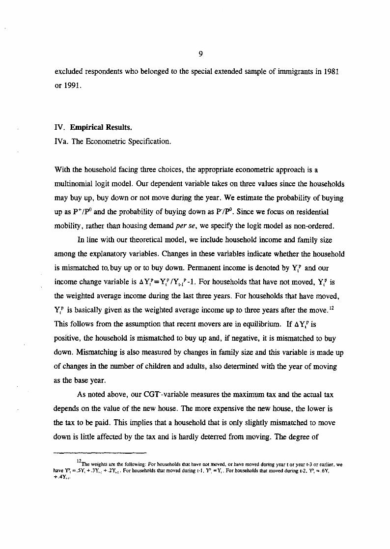
In line with our theoretical model, we include household income and family size

among the explanatory variables. Changes in these variables indicate whether the household

is mismatched to. buy up or to buy down. Permanent income is denoted by y t and our

income change variable is A y t = y t lYt} -1. For households that have not moved, ytp is

the weighted average income during the last three years. For households that have moved,

ytp is basically given as the weighted average income up to three years after the move. 12

This follows from the assumption that recent movers are in equilibrium. If A Y t is

positive, the household is mismatched to buy up and, if negative, it is mismatched to buy

down. Mismatching is also measured by changes in family size and this variable is made up

of changes in the number of children and adults, also determined with the year of moving

as the base year.

As noted above, our CGT-variable measures the maximum tax and the actual tax

depends on the value of the new house. The more expensive the new house, the lower is

the tax to be paid. This implies that a household that is only slightly mismatched to move

down is little affected by the tax and is hardly deterred from moving. The degree of

12The weights are the following: For households that have not moved, or have moved during year t or year t-3 or earlier, we have Y", =.5Y, +.3Y,., +.2Y,.,. For households that moved during t-l, Y", =Y,. For households that moved during t-2, Y", = .6Y, +.4Y,.,.

10

mismatching thus matters for the deterrence of CGT since buying a much cheaper house

would result in a large tax payment and buying a slightly cheaper house results in smaller

payment. Moreover , if the household experiences a rise in income CGT is not deterrent

since the household is expected to buy up. Define a variable Il Y- (suppressing the index t)

representing the degree of downward mismatch in permanent income (Il Y"). The variable

Il y- is the absolute value of Il Y". If Il YP is non-negative Il y- is set to zero. To capture the

dependence of the variable CGT on the degree of downward income mismatching, we

multiply CGT by Il Y-. We also allow for non-linearities in this variable by multiplying

CGT with the square of Il Y-.

Unlike the actual CGT the household pays after having adjusted to the tax rules, the

maximum amount of CGT is exogenous to the household and is the policy variable of

interest.

The taxes to be paid in case of buying up, CGT+, are, however, not dependent on

the price of the new house. Therefore, we multiply CGT+ with a dummy variable that

takes on a unit value when income has increased and zero otherwise. Similarly, we

interacted the family size variable and house prices with the CGT variables. House prices

are measured as the (real) regional house price index.

It seems reasonable to express capital gains taxes as a share ofcapital gains since a

large tax payment may be less prohibitive if the tax base itself is large. However, since

capital gains may be zero or negative, despite a positive tax, we included capital gains as a

separate variable in the analysis.

As noted in the theoretical section, trans action costs may also be of a psychic

nature. In our model, duration in the current dwelling and age of the head of household,

may be interpreted as proxies for such costs. Duration determines thestrength of

neighbourhood attachment that may inhibit mobility despite amismatch. Age may affect

the agony and physical strain of moving and also hamper mobility . These arguments imply

that duration and age should be included as proxies for psychic transaction costs in the

11

vectors T+ and 1. 13

Other interpretations of duration and age are possible in our framework. As a

moving household eliminates the gap between desired and actual housing consumption there

are no incentives to move directly after having bought a new house. However, the

household may acquire information about the new residence and its neighbourhood and

over time realize that it is mismatched. If so, duration should be included in the vector C as

a proxy for mismatching status. We test for these alternative interpretations by including

duration and age either in the T-variables or in the C vector.

Since the taxes partly depend on duration, including it as a separate variable allows

us to distinguish the effects of CGT from those of other transaction costs. As noted,

nominal gains were taxed during the frrst four years of ownership, real gains thereafter.

IV. b Sample Characteristics

We now tum to a description of some key variables in the data set. In Table 1 we present

statistics regarding residentiaI mobility . About one third of the households moved during

the period. There 'is a great deal of variation in mobility during the period. The highest

figure is for 1988, when 6.5 per cent of the households moved, and the lowest occurred in

1990, when only .9 per cent moved. During 1982-90, 12 per cent bought up and 18 per

cent bought down (not shown).

Table 1. Moving Households. Per cent.

1981 1982 1983 1984 1985 1986 1987 1988 1989 1990 1991 2.5 4.3 5.2 3.3 3.1 2.2 3.0 6.5 1.3 .9 4.3

13Duration and age are commonly included in empiricaJ studies on housing demand and residentiaJ mobiJity. but often without any explicit theoreticaJ basis.

12

Table 2 shows the real CGT for households in the sample. Recall that CGr­

represents the maximum tax payment, so the figures for CGr-and CGT+are not directly

comparable.

The variation in CGT depends on house price inflation, marginal taxes and changes

in the distribution between households with taxation on nominal and real gains. The

average CGT+ was very low in the period 1981-90, with values around SEK 1 000. Since

the maximum payment has been limited to SEK 15 000, relatively few h9useholds have

been subject to taxation. In 1991, when postponements were no longer allowed, CGT+

increased sharply from SEK 1 400 to 23300. Another important change was that

practically all households buying up became liable to taxation. Average CGr- has been

substantiai throughout the period, with considerable variation across the years

(SEK 7 300 - 26 800). There is also a great deal of variation across households, as seen in

the column showing the maximum values of CGr-. Between 34 and 68 per cent of the

households in the sample were subject to taxation until1991, when CGr- and CGT+ were

equalized. The

Table 2 Expected CapitaI Gains Taxes, in 1979 Prices (SEK).

Year CGT+ Share CGr- CGr- Share Mean CGT+>O Mean Max CGr-> O

1981 1,400 20 % 22700 342600 62 % 1982 1300 19 % 16400 165000 51 % 1983 1000 16 % 11300 118500 42 % 1984 900 14 % 8800 110000 36 % 1985 1000 15 % 7300 91400 34 % 1986 1100 16 % 8300 102100 36 % 1987 l 100 16 % 12100 136200 42 % 1988 1200 17 % 17900 211 900 50 % 1989 1300 21 % 25800 278,500 63 % 1990 1400 20 % 26800 256200 68 % 1991 23300 100 % 23300 88900 100 %

Note: The share figures represent the proportion of households that are liable to taxation. CGT+is the actual amount of taxes when buying up. whereas CGl is the maximum tax payment when buying down. The column CGl max expresses the highest maximum tax for any household.

13

tax reform in 1991 produced little change in average CGl as compared to the two previous

years, but all households became subject to taxation when buying down.

Table 3 contains data regarding some important variables for households who buy

up, buy down and for the whole sample. The data refer to the households included in our

estimations 1984-90. Those buying up are, on average, younger, have more children,

higher income and shorter duration in the current dwelling than those buying down.

Table 3. Sample Means.

Variable Households Households All buy~g up. buying down. households. At tlIDe of Att~ of Avera~e move.a move. 1984- 990. c

Age 44.9 49.1 49.0

No. children 2.2 2.0 2.0

Permanent incomei 63445 56423d 60 282e

Duration 8.7 9.8 17.2

CGT+ 462f 808g l 08~

CGr 9366f 14114g 15674h ·

Capital gains -8861 16696 22375

Notes: "65 households.bl07 households."3 648 observations (households x years). dl04 households.~ 563 observations. f64 households.'106 households. h3 575 observations. i Permanent income is defined as in text.

Although those buying Up on average make a capital loss they will pay a positive

capital gains tax. This, however, amounts to only SEK 462 which is slightly lower than for

those moving down had they decided to buy up, SEK 808. The maximum tax in case of

buying down is considerably higher; SEK 9 366 for those buying up had they decided to

buy down, and SEK 14 114 for those buying up.

14

IV.c The Regressions.

Before presenting the results, it is appropriate to discuss some estimation problems. First,

there is an obvious possibility of sample selection bias in the estimates. As mentioned in

Section III, we had to exclude households that moved more than once during the period,

since the CGT variables cannot be computed for this group. A standard method to deal with

such a sample selection bias is Heclanan's two-step procedure. We have performed

binomiallogit estimations on period-averages for the whole sample, where the dependent

variable indicates whether the household has moved or not moved during the period. As

explanatory variables we used household· income, family size, duration, duration squared

and age. Based on these cross-section estimates we have computed Heclanan' s A. for each

household and included this as a separate variable in the estimations in order to controi for

selection bias. 14

Secondly, there may be a problem with omitted variables that affect the household' s

propens ity to move. Some households in our sample may be more mobile than others, due

to e.g. unmeasured personal traits. If these omitted variables are correlated with the

included variables, our estimates will be biased. It is reasonable to assume that such

influences on mobility vary across households but are fIxed over time, so that a flXed­

effects specification is appropriate. The traditional method to controi for flXed effects is to

frrst-difference the data or introduce dummy variables. In models with discrete dependent

variables, however, this is not feasible. Instead we focus only on those households that

have moved during the period, and delete the observations for households that have not

moved. This enables us to controI for fIxed effects (see e.g. Baltagi, 1995, and Greene,

1993).

Table 4 shows the estimates with flXed effects for the probabilities of buying up and

buying down, respectively. (The corresponding estimates without consideration of flXed

effects are presented in an appendix.) Since non-moving

141t would have been preferable to inc\ude also CGr and CGT in the estimations of Heclanan' s ... However, these variables are not observed for households that have moved more !han once.

15

Table 4, Maximum-likelihood estimates of the multinomiallogit model, household panel data 1984-90, Dependent variables: The Oog of) probability to buy up and the

b bTt b d b th d' 'd d b th b bin t st Fix d f~ Ilro a l HV to uv own o IVl e ~V enro a HV o al, e e ects,

Variable Buyup Buy down

ex y ex y

Constant -12.3101 *** -7.6610*** (2.226) (1.926)

Chan~ in pennanent 1.1891** 0.03988 0.6598 0.03151 house old mcome (0.560) (1.445)

Change in family size 1.5883*** 0.05357 0.7297 0.03432 (0.456) (0.499)

CGT+ x dummy -0.12 -0.0040 -0.10 -0.0049 for increased income x 1000 (0.127) (0.071)

CG! x decreased income x 1.16 0.0418 -0.82** -0.0443 1000 (0.838) (0.404)

CG! x decreased income -0.0163 -0.000570 0.0028- 0.000175 squared (0.016) (0.001)

Capital gain x 1000 000 -8.39*** -0.28989 -0.287 0.0016 (3.218) (2.734)

C1}ange in regional house 1.9392 0.0739 -3.4584* -0.1811 pnces (2.177) (1.909)

Duration in current dwelling 1.2059*** 0.0398 1.0256*** 0.0502 (0.255) (0.198)

Duration squared -0.0431 *** -0.0014 -0.0324**· -0.0016 (0.013) (0.009)

Age 0.0026 0.00007 0.0105 0.00053 (0.018) (0.015)

Heclcman's Å 0.1645 -0.2415 (0.804) (0.822)

I Likelihood ratio

I 2916

1476 . No. observatIOns

Notes: Only those households that have moved during the period are included in the sample. Coefficient estimates are denoted by ex and slope estimates by y. Year dummies are included in all regressions. Standard errors in parentheses .• = significance at the 10 per cent level, ,. = 5 per cent, , .. = 1 per cent.

I

16

households have been excluded, and after having accounted for the fact that permanent

income depends on income lagged up to three years, the sample size is reduced from 4536

to l 476 observations over the period 1984-90. We excluded 1991, since we suspected the

classification of households buying up and buying down to be unreliable for this

year. 15

As the coefficient estimates (ex) in Table 4 are not easily interpreted we also present

the slope estimates (y). 16 The latter show how much the probability to buy up (or down) is

changed from a unit increase in a variable (see, for instance, Greene, 1993).

Increases in permanent income yield a significant and positive effect on the

probability to buy up. As the change in permanent income rises by l percentage unit, the

probability rises by .04. Decreases in income, however, do not seem to increase the

probability to buy down. A possible interpretation of this result is that households in

general have large enough margins for income los ses and are not forced to move when

incomes fall. 17

Increases in family size produce an expected increase in the probability to buy up.

As the change in family size increases by l percentage unit, the probability of moving to a

more expensive (and presumably larger) house rises by .05. Also, capital gains affect

residential mobility by unexpectedly lowering the propensity to move up.

The duration variables exert a significant influence on the probabilities of moving.

Our specification of the duration variables implies that duration is treated as a household

characteristic and not as an integral part of the transaction costs. (See Section IV.a.) This

interpretation is supported in the regressions. An increase in duration raises the probability

of buying up and the probability of buying down at decreasing rates. The estimates of the

duration variables thus imply a hump-shaped pattem, which is in line with several studies

that deal with the determinants of housing demand.

15 We do not know whether the households !hat have rnoved during 1991 have reported the assessed tax values of their houses before or after the rnove.

16 Standard errors are presente<! for coefficient estimates only and may be different for slope estimates.

17SUCh incorne margins would normally be a requirernent for obtaining the necessary loans for the house.

17

Consider now the effects of capital gains taxes. It can be noted that the estimates

where CGY- is multiplied by decreased income (Le. with the degree of mismatching to

buy down) yields a significant estimate of the expected negative sign on the probability of

buying down. Also, non-linearities are present. The total effect, including the non­

linearities, implies that if CGT rises by SEK 1 000, the probability of buying down falls

by .00031 (not shown in the table). As expected, the decision to buy up is unaffected by

CGT.

The estimates concerning the probability to buy down thus imply that the effects of

taxation depend on the degree to which the household is mismatched to buy down. In

Figure 1, we have plotted the effect on the probability of buying down following a 1 per

cent increase in CGT against the degree'of mismatching. 18 The absolute value of the

derivative increases at a decreasing rate as the degree of mismatching rises. While the

effect is small at the mean, .016, it is considerably larger when the degree of mismatching

approaches its maximum value in our sample, .41. The figure shows the lock-in effects

increase drastically in income mismatch and that large income reductions are necessary for

the tax to have a sizeable negative influence on residential mobility .

Are the effects we fmd small or large? The elasticity of the variable where CGT is

interacted with a decrease in income is -0.078 (the total effect) with respect to the decision

to buy down. The elasticities of changes in permanent income and family size with regard

to the decision to buy up are .025 and .006, respectively. Thus the tax effects are not at all

small when compared to the effects of other variables that commonly are considered in

analyses of residential mobility .

In the appendix we report the results obtained with the larger sample (4 536

observations), where fLXed effects have not been accounted for. In many cases the estimates

are now quite different. The effects of capital gains taxes are, though, fairly robust. As in

the fLXed effects regression, we fmd that an increase in CGT lowers the probability to buy

down and the effect depends on the degree of income mismatch. Moreover , as in the fLXed

effects regression, CGT+ does not seem to affect the probability to move in either

direction. These results show the importance of accounting for the fLXed effects.

18 As explained in Section IV.a, A y- assumes a zero value for a household with increasing income.

18

We have performed several additional regressions (available on request). Previously

we argued that duration and age also may act as proxies for transaction costs. We therefore

interacted these variables with the degree of mismatch. Compared to the results in Table 4,

the effects of taxes were very similar and the estimates of the transformed duration

variables were also highly significant. One may thus argue that duration can affect

residentiai mobility as a household characteristic as in Table 4 (by making the household

mismatched) as well as representing transaction costs. It should be recognized, however,

that composition effects may make the interpretation of the duration estimates difficult.

In creating a data set like the present one, there are naturally risks for measurement

errors. For instance, we have assumed that the assessed tax value reflects the true market

value of the house. This may not necessårily be so. While we have quite accurate data on

wlrich households that have moved, there may be cases where a household buying up

(down) is incorrectly c1assified as buying down (up). The risk for measurement errors is

naturally larger for those households that have made only small changes in housing

consumption. Relatively few households have made small changes. In our data, 13 per cent

of those buying up, bought up less than 5 per cent, while 11 per cent of those buying

down, bought down less than 5 per cent.

V. Concluding Remarks.

We have calculated the capital gains taxes applicable when moving to a more expensive

house and when moving to a less expensive one. This has been done for households in the

Level of Living Surveys and the data have been described at some length. We believe that

such data are of interest in their own right since there is very little information on the

transaction costs in the housing market. Our data obviously have a variety of applications

and in this paper we have estimated the effects of CGT on residentiaI mobility .

Our approach is based on the notion that residential mobility is driven by

households becoming mismatched. The empirical results concerning changes in income and

family size are, in general, supportive of this model. Assuming that CGT only matters if

the house-owner has been mismatched due to changes in income, we found that higher

19

taxes for those mismatched to buy down (in terms of lower income) reduce the probability

to buy down. The effect of the taxes on the probability of buying down depends on the size

of the income loss, Le. on the degree of mismatching. Given that the taxes in the case of

buying up are low and never exceed SEK 15 000, we were not surprised to fmd that this

tax does not affect residential mobility .

Our results highlight the importance of distinguishing the transaction costs involved

in buying down from those applicable when buying up. Moreover, it is necessary to take

into account the degree of mismatch when analyzing the effects of CGT. These aspects

have largely been ignored in the previous literature on residentiai mobility .

The elasticity of residentiai mobility with respect to capital gains taxes is not

negligible and comparable to those obtamed for other variables like changes in income and

family size. Still, one should remember that even if CGT is abolished, other transaction

costs remain that hamper residential mobility .

20

REFERENCES

Baltagi, B.H., (1995), Econometric Analysis of Panel Data. Wiley.

Börsch-Supan, A., (1990), "Panel Data Analysis of Housing Choices. " Regional Science and Urban Economics, 20, 65-82.

Börsch-Supan, A. and H.O. Pollakowski, (1990), "Estimating Housing Consumption Adjustments from Panel Data." Journal of Urban Economics, 27, 131-150.

Edin, P.-A. and P. Englund, (1991), "Moving Costs and Housing Demand. Are Recent Movers Really in Equilibrium?" Journal of Public Economics, 44, 299-320.

Englund, P., (1985), "Taxation of Capital Gains on Owner-Occupied Homes. Accrual vs Realization." European Economic Review, 27, 311-334.

Englund, P., (1986), "Transactions Costs, Capital-Gains Taxes, and Housing Demand. " Journal of Urban Economics, 20, 274-290.

Eriksson, R. and R. Åberg (eds.), (1987), Welfare in Transition, Oxford: Clarendon Press.

Greene, W.A., (1993), Econometric Analysis, second ed. Macmillan.

Hanushek, E.A. and J.M. Quiqley, (1979), "The Dynamics of the Housing Market: A Stock Adjustment Model of Housing Consumption." Journal of Urban Economics, 6, 90-111.

Lundborg, P. and P. Skedinger (1995), "Taxation in a Search Model of the Housing Market, " mimeo, Industrial Institute for Economie and Social Research, Stockholm.

SOU 1985:38, (1985), Reavinstuppskov. Fastigheter. Stockholm.

SOU 1989:33, (1989), Reformerad inkomstbeskattning. Stockholm.

Wheaton, W.C., (1990), "Vacancy, Search and Prices in a Housing Market Matching Model." Journal of Political Economy, 98, 1270-1292.

21

APPENDIX

Table A.l.MaxiInwn-likelihood estimates of the multinomiallo~t model, household panel data 1984-90. Dependent variables: The (log of) probability to buy up and the probability to buy down, both divided by the probability to stay.

Variable Buyup Buy down

(X y (X y

Constant -10.5010*** -8.0299*** (1.857) (1.538)

Chan~ in pennanent 0.5367 0.00652 -1.5422 -0.02683 house old mcome since last (0.764) (1.589) move

Change in family size since 0.3777 0.00443 -0.3377 -0.005929 last move (0.303) (0.494)

CGT+ x dummy for increased -0.1 -0.0011 -0.04 -0.00067 income x 1000 (0.122) (0.066)

CGl x decreased income x 0.983 0.01149 -0.67* -0.01181 1000 (0.688) (0.352)

CGl x decreased income -0.0131 -0.000152 0.0020** 0.0000380 squared (0.0126) (0.001)

Capital gain x 1000 000 1.773 0.0188 8.051*** 0.1391 (2.711) (2.011)

Cl?-ange in regional house -1.3360 -0.01442 -4.8818*** -0.0843 pnces (1.699) (1.499)

Duration in current dwelling 0.8993*** 0.01022 0.8224*** 0.01406 (0.214) (0.156)

Duration squared -0.0484**- -0.000550 -0.0423*** -0.000723 (0.011) (0.007)

Age 0.0026 0.0000238 0.0290** 0.000502 (0.017) (0.013)

Heckman's Å 0.5540 0.5675 (0.533) (0.405)

T llr.:,,1ihnnrf rlltin o (\'t;:;;

Nn .1- 4 ,'t;:;;

Notes: Coefficient estimates are denoted by IX and slope estimates by y .• = significance at the 10 per cent level:· = 5 per cent, 000 = 1 per cent. Year dummies are included in all regressions. Standard errors in parentheses.

Figure 4.1 Lock-in effects and mismatching. Effects on the probability of buying down of a 1 per cent increase in capital gains taxes (CGT -) at various income reductions.

(dP7dCGT-}*CGT-

0.000

-.001

-.002

-.003

-.004

~ '"

o 0.016

.1

~ ~

" ~~

.2 .3 .4 0.41

Note: .016 is the average income reduction and .41 the maximum.