nnumerical investigation of bubble interaction mechanisms
TRANSCRIPT
International Journal of Multiphase Flow 144 (2021) 103781
Available online 8 August 20210301-9322/© 2021 Elsevier Ltd. All rights reserved.
nNumerical investigation of bubble interaction mechanisms in gas-liquid bubbly flows: Harmonisation of bubble breakup and coalescence effects
S. Yamoah a,b,*, Castro K. Owusu-Manu a, Edward.H.K. Akaho a
a School of Nuclear and Allied Sciences, University of Ghana, P.O. Box AE1, Accra, Ghana b Ghana Atomic Energy Commission, Nuclear Power Institute, P.O. Box LG80, Legon, Accra, Ghana
A R T I C L E I N F O
Keywords: Population balance model Coalescence Breakup Two-phase flow Bubbly flow Two-fluid model
A B S T R A C T
Numerical investigation of the dynamics of gas-liquid bubbly flow has been performed by using the population balance approach. Using the homogeneous MUSIG model coupled with the two-fluid model, the evolution of bubble size distribution in vertical pipes has been simulated with appropriate consideration of bubble interaction mechanisms. In particular, the study focuses on harmonising the imbalance often associated with breakup and coalescence rates by performing extensive numerical investigations for the examination and comparison of different model formulations to harmonise the coalescence calibration factor of Prince and Blanch (1990) model. To avoid the fine-tuning procedure of selecting calibration factors to harmonise the breakup and coalescence effects, a breakup calibration factor of 1.0 (default setting in ANSYS CFX) was used and three different ex-pressions area-averaged and included as the coalescence calibration factor for the model of Prince and Blanch (1990) modelled using CFX Expression Language (CEL). The performance of the three different “cases” (modi-fications) has been investigated, compared with each other and validated against the experimental data reported by Monros et al. (2013). In general, the comparison has shown that all the “cases” yielded satisfactory results when the numerical results were compared with five primitive experimental parameters, namely: gas volume fraction, interfacial area concentration, Sauter mean bubble diameter, gas velocity and liquid velocity. The encouraging results obtained clearly show the capability of the “cases” modelled in capturing the evolution of the bubble sizes. The agreement with the gas volume fraction profiles indicates a level of confidence in the interfacial force models used. Similarly, the agreement seen with the interfacial area concentration indicates that the “cases” modelled for the birth and death processes are reasonably adequate to describe the bubble dynamics. Overall, the comparison shows that the model labelled as “case 2” presented the best results in most of the experimental conditions simulated.
1. Introduction
Gas-liquid two-phase flows have received extensive research in academia. It plays a crucial role in numerous industrial applications. These include power generation, transport of oil and gas, energy con-version, and safety technology in power plants, paper manufacturing, and food processing as well as nuclear applications. For gas-liquid mixture flowing in vertical pipe, variety of flow patterns may be observed, mostly bubbly (i.e. bubble flow at low liquid flow rates and dispersed bubble flow at high liquid flow rates), slug, churn and annular flows. In many instances, the observed regime is predominantly gov-erned by flow parameters and their relative magnitudes of both phases, the properties of the fluid, the pipe size and the bubble mechanistic
behaviours such as bubble breakup and coalescence. The internal flow structure of gas-liquid mixture flowing in vertical
pipes, are characterised by the gas volume fraction, interfacial area shared by the two phases, and mean bubble diameter. The gas volume fraction is used for hydrodynamics and thermal design in industrial processes. The interfacial transport of mass, momentum, and energy corresponds to the interfacial area and the driving force. These param-eters are very crucial for a two-phase flow model formulation. The mean bubble diameter stands in to connect the gas volume fraction and interfacial area concentration. Understanding the transfer processes of these parameters is important for effective numerical simulation of gas- liquid two phase flows (Kocamustafaogullari and Huang, 1994).
The interfacial area concentration can be represented by the bubble
* Corresponding author. E-mail address: [email protected] (S. Yamoah).
Contents lists available at ScienceDirect
International Journal of Multiphase Flow
journal homepage: www.elsevier.com/locate/ijmulflow
https://doi.org/10.1016/j.ijmultiphaseflow.2021.103781 Received 5 May 2020; Received in revised form 17 March 2021; Accepted 5 August 2021

International Journal of Multiphase Flow 144 (2021) 103781
2
number in a certain spatial volume called number density. For gas-liquid flows, the population balance model is able to track the bubble number as it changes in finite space under the consideration of bubble breakup and coalescence due to interaction among bubbles and turbulent eddies (Hibiki and Ishii, 2002). To consider the phenomenon of bubble breakup and coalescence, the population balance method in the form of MUSIG model has been adopted in this study coupled with the two-fluid modelling framework. Extensive studies have been carried out and re-ported in literature on the population balance modelling (Olmos et al., 2001; Chen et al., 2005; Wang et al., 2006; Zucca et al., 2006; Cheung et al., 2007a,b, 2008; Ekambara et al., 2012; Liao et al., 2011; Cheung et al., 2013). This approach is concerned with maintaining a record of the number of bubbles initially and tracking their evolution in space over time.
Interactions of fluid particles leading to breakup in turbulent dispersion is affected by the hydrodynamics of the continuous phase and interfacial interactions. Liao and Lucas (2009) distinguished four cate-gories of fluid particles breakup mechanisms, namely: (a) turbulent fluctuation and collision; (b) viscous shear stress; (c) shearing-off pro-cess; (d) interfacial instability. In bubbly flow conditions as is the case in this study, breakup due to the impact of turbulent pressure fluctuations along the surface, or by particle-eddy collisions is considered. The breakup kernel function developed by Luo and Svendsen (1996) which considers turbulence eddy collision effect is adopted in this study to account for breakup of bubbles. The model assumes that bubble binary breakage is based on isotropic turbulence theories and that breakage of bubbles can only occur when the eddy bombarding has energy greater than the surface energy required for the breakage, a phenomenon known as energy constraint (Wang et al., 2003).
Coalescence is a complex phenomenon (Chesters, 1991) because it does not only involve bubbles interacting with surrounding liquid, but also among bubbles themselves. Three theories have been proposed in literature to account for coalescence processes. Among them is the film drainage model proposed by Shinnar and Church (1960). According to this model, the coalescence process can be grouped into three sub-processes, namely: (a) two bubbles collide, trapping a small amount of liquid between them; (b) bubbles keep in contact till the liquid film drains out to the critical thickness; and (c) the film raptures resulting in coalescence. Howarth (1964) on the other hand, argues that for coa-lescence to occur will depend on the impact of the colliding bubbles. This according to Howarth is because the attraction force of two colliding interfaces is too weak compared with the turbulent force. Recently, Lehr and Mewes (1999) and Lehr et al. (2002) introduced the critical approach velocity model by indicating that small approach ve-locities would lead to high coalescence efficiency. Contact and collision are the premise of coalescence.
For a turbulent bubbly flow, the relative motion that causes collision between bubbles may occur through mechanisms such as turbulent fluctuations induced motion in the continuous phase, motion caused by mean velocity gradients in the flow, different bubble rise velocities induced by buoyancy or body forces, bubble capture in an eddy, wake interactions or helical/zigzag trajectories (Liao and Lucas, 2010). Not all collision lead to coalescence, and most of them bounce back from each other after collision. Therefore, efficiency or probability of coalescence is introduced for computation of coalescence frequency. Different models (both physical and empirical) have been developed to account for coalescence frequency. In recent works as noted by Liao and Lucas (2010), some modifications have been proposed to account for (i) the effect of size ratio between bubbles and eddies and (ii) the existence of bubbles that reduces the free space for bubble movement and causes an increase in the collision frequency.
In this study, numerical investigation of gas-liquid bubbly flows has been performed by coupling population balance model with the three- dimensional, two-fluid model. A model validation study to account for non-uniformity of bubble size distribution using the MUSIG model in a highly asymmetrical distributed bubbly flow in the vertical pipe is
presented covering a wide range of gas and liquid superficial velocities. The focus of the study has been centred on the detailed numerical investigation of the coalescence phenomenon by performing extensive numerical investigations for the examination and comparison of different model formulations to harmonise the coalescence calibration factor.
To avoid the fine-tuning procedure of selecting calibration factors to harmonise the breakup and coalescence effects as reported in literature, the Prince and Blanch (1990) coalescence model has been modified considering the effect of size ratio between bubbles and eddies and the existence of bubbles that reduces the free space for bubble movement. These effects have been area-averaged and included as the coalescence calibration factor using CFX Expression Language (CEL) while the breakup calibration factor has been maintained as 1.0 (default setting in ANSYS CFX). Simulated results have been validated against experi-mental measurements reported by (Monros-Andreu et al., 2013) for gas volume fraction, interfacial area concentration, Suater mean bubble diameter gas and liquid velocities
2. Mathematical modelling
2.1. Population balance model
To account for the phenomenon of bubble coalescence and breakup, the population balance modelling (PBM) approach using the homoge-neous MUSIG model (Lo, 1996) was adopted in this paper. The formu-lation of the MUSIG model starts from the discretised population balance equation (PBE). It is possible to compute the bubble size distribution using the population balance equation expressed as:
∂ni
∂t+∇.(niui) =
∑
jRj (1)
Where ni is the bubble number density, ui is the velocity vector and ∑
jRj is the source term accounting for bubble coalescence and breakup.
To solve Eq. (1), Kumar and Ramkrishna (1996) approach was used by expressing the bubble number density in terms of size fractionfi of M bubble size groups as:
∂(ρgαgfi
)
∂t+∇
(ρgugαgfi
)= Si (2)
The term Siin Eq. (2) is a source term to account for the birth and death of bubbles of size i, which was expressed as:
Si = Bbi − Dbi + Bci − Dci (3)
where Bbi, Bcirepresents the birth of bubbles due to breakup and coa-lescence and Dbi,Dcirepresents the death of bubbles due to both breakup and coalescence. These terms were computed as expressed in Eqs. (4)– (7).
Bbi = ρjαj
(∑
j > iΩ(mj, mi
)fj
)
(4)
Dbi = ρjαj
(fi
∑Ω(mj, mi
))(5)
Bci =(ρjαj)2(
12∑∑
Γ(mj, mk
))
Xjkifjfkmj + mk
mjmk(6)
Dci =(ρjαj)2(∑
Γ(mi, mj
))fifj
1mj
(7)
where Ω(mi, mj)and Γ(mi, mj)are the breakup and coalescence kernel functions respectively.
The term Xjki in Eq. (6) is a coalescence mass matrix defined as the fraction of mass due to coalescence between groups jat t which goes into
S. Yamoah et al.

International Journal of Multiphase Flow 144 (2021) 103781
3
group i. This term is introduced to account for the contribution of birth rate due to coalescence and was expressed as:
Xjki =
{1 if mj + mk > mi
0 Otherwise (8)
The birth and death rates are commonly expressed in terms of breakup and coalescence kennels. Over the past decades, the phenom-enon of fluid particle breakup and coalescence have been the subject of attention both theoretically and experimentally. In this study, the breakup model of Luo and Svendsen (1996) which is based on the assumption of bubble binary breakup under isotropic turbulence has been used. The breakup rate of bubbles of volume vj into volume of sizes vi expressed in terms of mass was modelled as:
Ω(Mi,Mj
)= 0.923FB
(1 − αg
)(
εl
d2j
)13 ∫ 1
min
(1 + ξ)2
ξ113
× exp
{12cf σ
2ρl(εl)2/3d5/3
j ξ11/3
}
dξ
(9)
Where cf accounts for increased coefficient of surface area expressed as cf = [f2/3
bv +(1 + fbv)2/3
− 1] and ξ = λ/dj is the size ratio in the inertial sub-range between an eddy and a particle and thus, ξmin = λmin /dj. FB is a calibration factor. The parameter fbv is a dimensionless variable that accounts for the size of daughter bubbles or breakup volume fraction expressed as:
fbv =vi
v=
d3i
d3 =d3
i
d3i + d3
j(10)
where di and dj corresponding to vi and vj are daughter bubbles di-ameters and d which correspond to v is the parent bubble diameter that breakes into di and dj in the binary breakup.
The coalescence process involves interactions of bubbles with sur-rounding liquid and bubble-bubble interactions once they are put together by the body forces. This may occur as a result of turbulent random collision, wake entrainment and buoyancy. For the present study, only coalescence due to turbulent random collision was consid-ered. For turbulent bubbly flow as considered in this study, collision resulting from the fluctuating turbulent velocity of the surrounding liquid is considered as the most dominating factor. Thus, the coalescence rate according to Prince and Blanch (1990) can be considered as a product of collision rate and collision efficiency. This is expressed in terms of mass as:
ψ(Mi,Mj
)= FC
π4{
di + dj}2{
u2ti + u2
tj
}1/2exp(
−tij
τij
)
(11)
The time required for two bubbles to coalesce (τij) is computed based on the expression:
tij =
[(dij/
2)3ρl
16σ
]1/2
ln(h0/
hf)
(12)
While the actual contact time for two bubbles during the collision (τij) is evaluated as:
τij =
(dij/
2)2/3
ε1/3l
(13)
The equivalent diameter dij was evaluated according to suggestion by Chesters and Hofman (1982) as:
dij =
(2di+
2dj
)− 1
(14)
The turbulent velocity ut in Eq. (11) was evaluated according to the expression (Rotta, 1972):
ut =2
√(εld)1/3 (15)
ho and hf in Eq. (12) respectively represent initial and critical film thickness when collision begins and rapture occurs with assigned value of ho = 1x10− 4m and hf = 1x10− 8m (Prince and Blanch, 1990). FC is coalescence calibration factor.
From literature, it has been observed that breakup and coalescence rates are not the same. To account for the difference in the breakup and coalescence rates, researchers have fine-tuned the calibration factors FB and FC to match their experimental data. Olmos et al. (2001) used a calibration factor of 0.075 to enhance the breakup rates. Chen et al. (2005), enhanced the breakup rate by a factor of 10 in their numerical calculations. Duan et al. (2011) used factors FB = 0.25 and FC = 0.05 for the inhomogeneous MUSIG model and factor FB = 0.25 and FC = 0.10 for the average bubble number density model respectively. Yamoah (2014), used a coalescence factor of FC = 0.05 and break-up factor of FB = 0.2 to improve the coalescence and breakup rates. With focus on coalescence phenomena, the Prince and Blanch (1990) model has been implemented in this study with modification. Instead of specifying a constant value for the coalescence calibration factor, different expressions that take into account the volume fraction of the bubble have been modelled using CFX Expression Language (CEL). Three cases have been investigated to account for the coalescence calibration factor as explained below.
Liao (2010) extensively reviewed bubble coalescence mechanisms and reported of modification factors that have been proposed in recent works. The first proposed modification factor account for the effect of size ratio between bubbles and eddies. Colin and Riou(2004), argued that turbulence-induced collision may occur only in the following cases:
(di < le; dj < le
), urel =
Ct1.61
√
(
ε di + dj
2
)1/3
(16a)
(di〈le; dj
〉le), urel =
Ct1.61
√ (εdi)1/3 (16b)
where the coefficient, Ct takes into account the difference between the velocity of bubbles and the eddies, which has been neglected previously, while the factor 1/
1.61
√considers the deceleration of the approaching
bubbles due to an increase in their mass (Liao, 2010). The second modification factor considers the phenomenon of
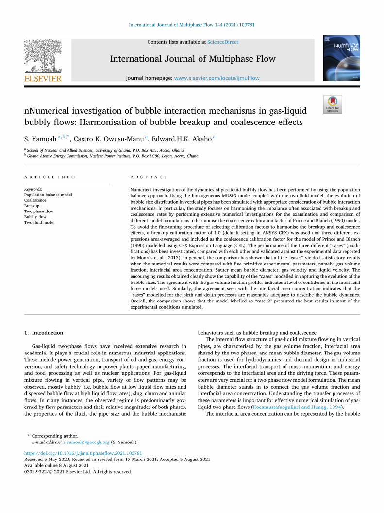
increased collision frequency of bubbles due to reduction in space for bubble movement resulting from existence of other bubbles. To address this effect, the collision frequency is multiplied by a factor, γ. Different expressions of factor γ summarised in Table 1 can be found in literature.
A plot of the dependence of factor γ on the volume fraction is shown below (Fig. 1). From the Figure, it is observed that the expressions have similar form. The dependence of γ for low gas phase fraction is small but takes infinite value when the packing of particles approaches the maximum. The only exception to the above is Lehr et al. (2002) where the exponential nature of the expression makes it inconsistent with the definition of factor γ.
The third modification factor reported in literature concerns the ratio of bubble mean distance to the average relative turbulent path length of bubbles. Wu et al. (1998) and Wang et al. (2005a) proposed that colli-sion is effective when the distance between bubbles is less than the
Table 1 Different expressions for factor γ (Liao, 2010).
Factor γ αmax Reference
1α1/3
max(α1/3max − α1/3)
0.8 Wu et al. (1998)
1αmax − α
0.52 (2000a) 0.741 (2000b)
Hibiki and Ishii (2000a, 2000b)
exp
[
−
(α1/3
max − α1/3
α1/3
)2] 0.6 Lehr et al. (2002)
αmax
αmax − α 0.8 Wang et al. (2005a, 2005b)
S. Yamoah et al.
International Journal of Multiphase Flow 144 (2021) 103781
4
turbulent path length. Thus, a decreasing factor Π should be added to Eq. (16). Subsequently, Wu et al. (1998) proposed the following modifica-tion factor by assuming that the average size of eddy is to be on the same order of the bubble size.
Π =
[
1 − exp(
− C16It
hb,12
)]
=
[
1 − exp
(
− Cα1/3
max α1/3g
α1/3max − α1/3
g
)]
(17)
where C = 3 is an adjustable parameter, depending on the properties of the fluid.
Wang et al. (2005a, b) on the other hand proposed that the factor Π should approach unity when the ratio hb,12/lbt,12 is small and zero when the ratio is large so that:
Π = exp[
−
(hb,12
Ibt, 12
)6]
(18)
where lbt,12 is the mean relative turbulent path length of bubbles of size d1 and d2.
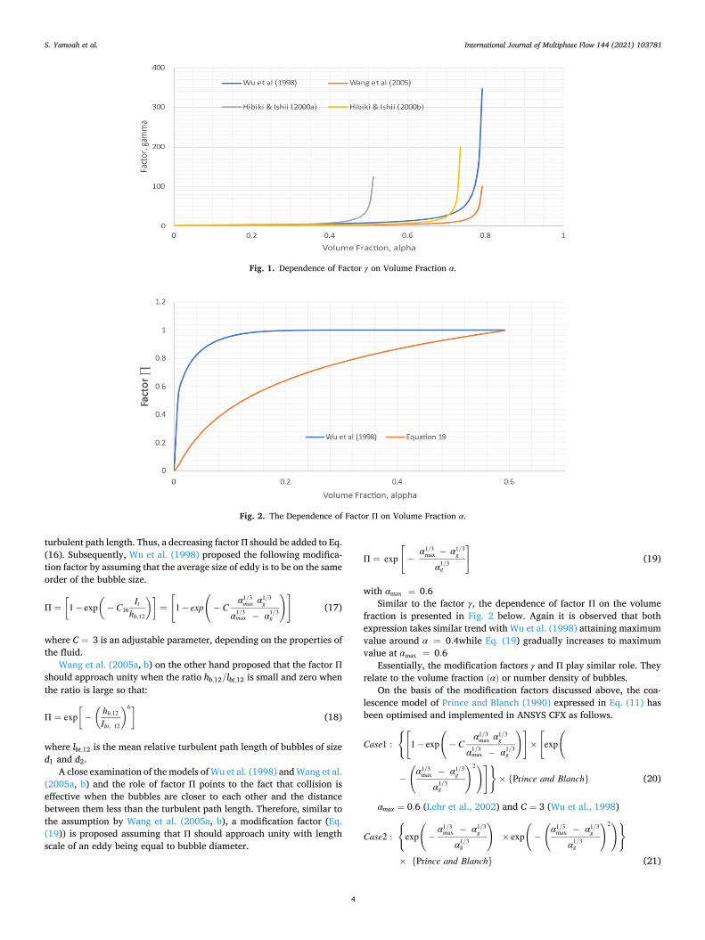
A close examination of the models of Wu et al. (1998) and Wang et al. (2005a, b) and the role of factor Π points to the fact that collision is effective when the bubbles are closer to each other and the distance between them less than the turbulent path length. Therefore, similar to the assumption by Wang et al. (2005a, b), a modification factor (Eq. (19)) is proposed assuming that Π should approach unity with length scale of an eddy being equal to bubble diameter.
Π = exp
[
−α1/3
max − α1/3g
α1/3g
]
(19)
with αmax = 0.6 Similar to the factor γ, the dependence of factor Π on the volume
fraction is presented in Fig. 2 below. Again it is observed that both expression takes similar trend with Wu et al. (1998) attaining maximum value around α = 0.4while Eq. (19) gradually increases to maximum value at αmax = 0.6
Essentially, the modification factors γ and Π play similar role. They relate to the volume fraction (α) or number density of bubbles.
On the basis of the modification factors discussed above, the coa-lescence model of Prince and Blanch (1990) expressed in Eq. (11) has been optimised and implemented in ANSYS CFX as follows.
Case1 :
{[
1 − exp
(
− Cα1/3
max α1/3g
α1/3max − α1/3
g
)]
×
[
exp
(
−
(α1/3
max − α1/3g
α1/3g
)2)]}
× {Prince and Blanch} (20)
αmax = 0.6 (Lehr et al., 2002) and C = 3 (Wu et al., 1998)
Case2 :
{
exp
(
−α1/3
max − α1/3g
α1/3g
)
× exp
(
−
(α1/3
max − α1/3g
α1/3g
)2)}
× {Prince and Blanch} (21)
Fig. 1. Dependence of Factor γ on Volume Fraction α.
Fig. 2. The Dependence of Factor Π on Volume Fraction α.
S. Yamoah et al.

International Journal of Multiphase Flow 144 (2021) 103781
5
αmax = 0.6 (Lehr et al., 2002)
Case3 :
{
exp
(
−α1/3
max − α1/3g
α1/3g
)
x(
αmax
αmax − αg
)}
x {Prince and Blanch}
(22)
αmax = 0.8 (Wang et al., 2005a)
2.2. Conservation equations
The two-fluid Eulerian-Eulerian model is used in this study to numerically solve the ensemble-averaged mass and momentum trans-port equations governing each phase. The liquid phase is considered as the continuum and denoted by (αl) and the gas phase (i.e. bubbles) is considered as disperse and denoted by (αg). These equations can be written as follows:
Liquid phase continuity equation
∂∂t(ρl αl) + ∇⋅(ρl αl ul) = 0 (23)
Gas phase continuity equation
∂∂t(ρg αg
)+ ∇⋅
(ρg αg ug
)= 0 (24)
Liquid phase momentum equation
∂∂t(ρl αl ul) + ∇⋅(ρl αl ul ul) = − αl∇P + αl ρl g
+ ∇{
αl μel
(∇ul + [∇ul]
T)}+ Flg
(25)
Gas phase momentum equation
∂∂t(ρg αg ug
)+ ∇⋅
(ρg αg ug ug
)= − αg∇P + αg ρg g
+ ∇{
αg μeg
(∇ug +
[∇ug
]T)}+ Fgl
(26)
Where μel and μe
g are the effective viscosities of the liquid and gas phases. The terms appearing on the right-hand side of Eqs. (25) and (26) describes different forces acting on the phases. These are the pressure gradient, gravity, viscous stress and interfacial forces. The interfacial force Flg represent the sum of forces made up of drag and non-drag (lift, wall lubrication and turbulent dispersion) forces that affect the interface between each phase. The total interfacial force is expressed as:
Flg = − Fgl = Flgdrag + Flg
lift + Flgwall + Flg
dispersion (27)
The drag force presents resistance between bubbles of the dispersed phase and the continuous phase and is computationally expressed ac-cording to Ishii and Zuber (1979) as:
Flgdrag =
18
CD ai ρl
ug − ul
(ug − ul
)(28)
The lift force acts perpendicular to the main flow direction and is expressed according to Drew and Lahey (1979) as:
Flglift = CLαgρl
(ug − ul
)x (∇ x ul) (29)
The model of the wall lubrication force used in this study is based on the expression of Antal et al. (1991) as:
Flgwall = −
αg ρl[(
ug − ul)−( (
ug − ul)nw)nw]2
ds
(
Cw1 + Cw2ds
yw
)
nw
(30)
For turbulent dispersion force, the model of Lopez de Bertodano (1991) was used and is expressed as
Flgdispersion = − CTDρlel∇αg (31)
elis the turbulent kinetic energy in the continuous phase.
Fig. 3. Computational domain.
Fig. 4. Effect of grid size on gas volume fraction and interfacial area concentration.
Table 2 Flow conditions of experiment simulated in this study (Monros et al., 2013).
Test Jl (m s− 1) Jg (m s− 1)
VL05JG005TA 0.50 0.05 VL05JG010TA 0.50 0.10 VL05JG030TA 0.50 0.30 VL10JG005TA 1.00 0.05 VL10JG010TA 1.00 0.10 VL10JG030TA 1.00 0.30
S. Yamoah et al.

International Journal of Multiphase Flow 144 (2021) 103781
6
The drag coefficient CD in Eq. (28) was modelled according to the correlation of Grace (1976). The lift coeffieicnt CL was modelled base on Tomiyama (1998) with modification of the aspect ratio. According to Tomiyama (1998) the coefficient CL can be expressed as a function of Eotvosnumber (Eo) as:
CL= {
min[0.288tanh
(0.12 Reg
); f (Eod)
]Eo < 4
f (Eod) = 0.00105Eo3d − 0.0159Eo2
d − 0.0204Eod + 0.474 4 ≤ Eo ≤ 10− 0.29 Eo > 10
(32)
Where Eod is the modified Eotvosnumber expressed as
Eod =g(ρl − ρg
)d2
H
σ (33)
In Eq. (33), dHis the maximum horizontal bubble diameter and was expressed according to the correlation (Yamoah et al., 2015)
dH = ds
(
2+1 + (Eo − 0.05)2.3
0.5(1 + 0.26Eo1.6)
)
(34)
The constants Cw1 and Cw2 in Eq. (30) was set at -0.01 and 0.05 respectively according to Antal et al. (1991). The turbulent dispersion force coefficient CTD in Eq. (31) was set to 0.5
Many turbulent models have been proposed to compute the turbu-lence viscosity such as k − ε model, k − ω model, their extensions Shear Stress Transport (SST) model. In single-phase flow, the standard k − ε model is generally used because of its simplicity and stability (Menter, 1994). However in multi-phase flow, no standard turbulence model is suitable for all flow conditions. Cheung et al. (2007a) noted that the Shear Stress Transport (SST) model developed by Menter (1994), was found superior to the standard k − ε model. Thus, the SST model is used in this study. The model applies the k − ω model near the wall and the k − ε model in the bulk flow.
Fig. 5. Sensitivity of the number of size groups.
Table 3 Diameter of each bubble class tracked in the simulation.
Class index 1 2 3 4 5 6 7 8 9 10
Bubble Diameter, Db (mm) 1.25 2.20 3.15 4.10 5.05 6.00 6.95 7.90 8.85 9.80
Fig. 6. . The dependency of turbulent collision frequency on the bubble size.
S. Yamoah et al.

International Journal of Multiphase Flow 144 (2021) 103781
7
Sato et al. (1981) bubble-induced turbulence model is used in this study to account for the contribution of turbulence in the liquid phase due to existence of dispersed phase bubbles. Thus, the dynamic viscosity of the liquid phase considering the production and destruction of liquid turbulence due to agitation of bubbles was expressed as (Sato et al., 1981):
μt,l = μts,l + μtd,l (35)
where the the shear-induced turbulence is expressed as μts,l = Cμρlk2l /εl
and the bubble-induced turbulence is expressed as μtd,l = Cμpρlαgdsug −
ul. The constants Cμ and Cμp are respectively specified as 0.09 and 0.6
Fig. 7. . The dependency of turbulent collision frequency on the bubble size.
Fig. 8. Radial gas volume fraction profile compared to experimental data.
S. Yamoah et al.

International Journal of Multiphase Flow 144 (2021) 103781
8
for bubbly flow regime. The gas phase turbulent viscosity was accounted for using the
dispersed phase zero equation model which can be expressed as
μt.d =ρg
ρl
μt,l
Prtg(36)
wherePrtgis the turbulent Prandtl number of the gas phase. Its value is set to unity.
3. Numerical solution
Numerical solution was performed using commercial computational fluid dynamics code ANSYS-CFX14.5 (CFX-14.5, 2012). The experi-mental facility simulated is described in detail by (Monros et al., 2013). Experiments were carried out in an upward air-water flow configuration to study the effects of temperature variation in bubbly and bubbly to slug transition flows. The test section is a round transparent tube of inner diameter D = 52 mm and and length L = 5500 mm. Measurements were taken at three axial locations of 1166 mm (Low Port, L/D=22.4), 3176 mm (mid Port, L/D=61) and 5131 mm (Top Port, L/D=98.7). Numerical calculations were performed on a 5-degree radial sector of the pipe (Fig. 3) allowing symmetry boundary conditions to be imposed at both vertical sides of the computational domain. A number of researchers have used 5-degree calculation mesh to simulate experiments related to upward vertical bubbly flow conditions (Sari et al., 2009; Liao et al., 2011; Pellacani, 2012; Yamoah et al., 2015). A mesh sensitivity analysis
was conducted to determine the effect of different grids on the numerical results by varying both radial and axial elelments of the computational domain as shown in Fig. 4. It can be observe that the results obtained by “mesh B” when validated with the volume fraction of the dispersed phase and the interfacial area concentration presented the most acceptable grid resolution. Therefore the numerical investigations in this study has been performed with the selection of a hexahedral mesh of 27 uniform radial elements and 411 uniform axial elements over the entire pipe domain giving a total of 21,783 nodes. Simulations were performed for combinations of gas and liquid superficial velocities at axial location L/D = 98.7 as shown in Table 2.
Key to the success of this method is the number of size groups used for the simulation and the size group fractions. To find an ideal number of size groups required to describe a meaningful distribution and for a more precise measure of the interfacial area density, sensitivity of the number of size groups was investigated (Yamoah, 2014) by dividing the bubble diameters equally into 5, 10, 15, and 20 size groups. The outcome of the investigations (Fig. 5) showed that, not much difference was found for the predicted gas volume fraction, interfacial area con-centration, Sauter mean bubble diameter, gas velocity and the liquid velocity and that the subdivision into 10 size groups was satisfactory (Table 3)
The measured radial profiles of gas volume fraction, liquid and gas velocities were set as inlet boundary condition in accordance with flow conditions whilest the outlet boundary was set to atmospheric pressure. A non-slip boundary condition was set for the liquid phase and a free-slip
Fig. 9. Comparison of interfacial area concentration profile with experimental data.
S. Yamoah et al.

International Journal of Multiphase Flow 144 (2021) 103781
9
boundary condition for the gas phase was set on the walls assuming that direct contacts between the bubbles and the walls are negligible.
In other to avoid the fine-tuning procedure of selecting calibration factors to harmonise the coalescence and breakup effects, a breakup calibration factor of 1.0 was used (default setting in ANSYS CFX) and the three different expressions Eqs. (20)–((22)) area-averaged and included as the coalescence calibration factor for the Prince and Blanch (1990) model. This was maintained for all the simulations. For all flow condi-tions simulated in this study, reliable convergence criterion based on the root means square (RMS) residual of 1× 10− 4was adopted for the termination of numerical calculations.
4. Results and discussion
In Figs. 6 and 7, it is possible to see how different combinations of the modification factors affect the trend of the random collision frequency. In Fig. 6, the random collision frequency of Prince and Blanch (1990) that takes into account the combination of modification factors, “case 1”, “case 2”, and “case 3”, is presented. The lowest collision frequency values were obtained by “case 2”. In Fig. 7, a plot of random collision frequency with and without consideration of the modification factors is presented. It is observed that for all the three cases, the random collision frequency considering the modification factors is small compared with when the modification factors are not considered. This is especially the case for small bubbles because the mean distance between small bubbles is larger than between big ones if the bubble number is equal (Liao, 2010). However, with increasing bubble size, the difference reduces. For case 3, the trend changes with bubble size of approximately 0.8 m.
To assess the models within a wide range of flow scenarios, analysis has been carried out to test the modified coalescence model with six different experimental data that represent different combinations of gas and liquid superficial velocities. The results of the analysis are presented below.
4.1. Gas volume fraction
Fig. 8 shows the simulation results of gas volume fraction profile obtained from the three “cases” compared with experimental measure-ments for all the experimental conditions simulated in this study. It is generally observed that all the “cases” were able to capture the different flow regimes exhibited by the experimental data. The transition process of the gas volume fraction profile from wall peak to core peak were captured by all the “cases” reasonably. The capability of the models to reasonably predict the transition process demonstrate that the interfa-cial force models used was able to successfully predict the gas phase lateral motion trend and separation of large and small bubbles. For the experimental data labelled VL10JG005TA and VL10JG030TA, one can observe that the predicted gas volume fraction profile agrees very well with the experiment for all the three “cases”.
On the other hand, for the experimental data labelled as VL05JG010TA and VL010JG010TA, the predictions of “case 1 and case 3” were not as close as in the other experimental data. Overall, it is observed that the prediction of “case 2” for all the experimental condi-tions simulated provided better compararism with the experiment than “cases 1 and 3”.
Fig. 10. Comparison of predicted Sauter mean bubble diameter with experimental data.
S. Yamoah et al.

International Journal of Multiphase Flow 144 (2021) 103781
10
4.2. Interfacial area concentration
The simulated results of interfacial area concentration compared with experimental data is shown in Fig. 9. Similar to the observed trend for gas volume fraction profile, the overall prediction of the interfacial area concentration from the three “cases” is generally good. However, there are noticeable differences in some of the experimental condition, notably experimental conditions VL05JG030TA and VL10JG030TA.
One can also notice that for the experimental condition labelled VL10JG005TA predictions for all the three “cases” is in good agreement with the experimental data. The reason for the good prediction for this experimental condition could be due to a reasonably good prediction of the bubble diameter and gas volume fraction profile together with appropriate combination of interfacial force models. Again, it is observed that the breakup due to turbulent impact is lower than the absolute ratio of coalescence due to random collision and this happens near the wall. This behaviour leads to low values of the numerical pre-dictions near the wall region for interfacial area concentration, even when the predictions of the gas volume fraction are accurate. This observation is more associated with “cases” 1 and 3 in almost all the experimental conditions simulated except for VL05JG030TA and VL10JG030TA where all three cases gave low predictions of the inter-facial area concentration throughout the pipe domain. From the results obtained from Fig. 9, it can be said that the modelled expressions for coalescence gave good account of evolution of the bubble size distri-bution since all the “cases” generally showed good agreement with the experimental data. Again the overall prediction for “case 2” is
reasonably better compared to “cases” 1 and 3.
4.3. Sauter mean bubble diameter
Fig. 10 presents the results of Suater mean bubble diameter obtained from the simulation for all three “cases” in comparison with the exper-imental data. Here it is observed that in most of the experimental con-ditions simulated, the prediction of “case” 2 provided better satisfactory agreement with the experimental data when compared with “case” 1 and “case” 3. Nonetheless all three “cases” over predicted the experi-mental Sauter mean bubble diameter for the high superficial gas ve-locities (i.e. VL05JG030TA and VL10JG030TA). The dynamical changes of bubble size distribution dictates fundamentally the interfacial area shared between the gas and liquid phases, which is closely coupled with the interfacial momentum transfer and the gas volume fraction profile. The observed trend is that the difference between numerically simulated and experimental Sauter mean bubble diameter increases with increasing superficial gas velocity especially for “cases” 1 and 3. This phenomenon could be attributed to higher coalescence effect compared to breakup leading to higher bubble diameters. The potential tendency of small bubbles migrating towards the wall provides considerable possibility for highly concentrated bubbles to merge together to form slightly larger bubbles leading to high coalescence effects. Since the Sauter mean bubble diameter is generally closely coupled with the interfacial momentum forces (i.e. drag and lift forces), better predictions of the bubble diameter could significantly improve the prediction of liquid and gas velocities, the interfacial area concentration and the void
Fig. 11. Comparison of radial profiles of gas velocity.
S. Yamoah et al.

International Journal of Multiphase Flow 144 (2021) 103781
11
fraction. In addition, interfacial forces acting on swarm of bubbles are generally affected by the closely packed neighbouring bubbles. The experimental findings of Simonnet et al.(2007) revealed that the drag force acting on bubbles decreased significantly if the gas volume fraction exceeded the critical value around 15%. With reference to experimental condition VL05JG030TA and VL10JG030TA, the gas volume fractions at the core peak is about 42% suggesting that the neighbouring interstitial effect could become influential at the centre of the pipe.
Overall, the simulated results of Sauter mean bubble diameter were reasonably in good agreement with the experimental data, in particular for the experimental conditions labelled as VL05JG005TA and VL10JG005TA. The capability of the models (“cases”) to capture the dynamical changes is very significant in examining bubble breakup and coalescence models as the bubble sizes influences the interfacial area shared between the gas and the liquid phases. The interfacial area is closely coupled with the interfacial forces (especially drag and lift forces) and the gas volume fraction profile.
4.4. Gas velocity profile
The gas velocity profiles are shown in Fig. 11 for all the three “cases” together with the experimental data. The results generally indicate reasonable prediction of the experimental data. It is observed from the plots that no appreciable difference exists between the three “cases”
modelled except for the experimental condition VL05JG010TA and VL10JG010TA where there is noticeable difference between “case” 2 and “cases” 1 and 3. For the experimental condition VL05JG030TA, all the three cases predicted lower than the experimental value.
It can also be observed that for the experimental conditions with superficial liquid velocity of 1 ms− 1, all the simulated “cases” over predicted the gas velocity close to the wall region. However, in the core, the gas velocity were under predicted except for “case” 2 of VL10JG010TA. The reason for the observed trend could be due to lower sampling of the liquid flow field close to the wall thus causing the ve-locity profile not to smoothly fall to zero.
4.5. Liquid velocity profile
The liquid velocity profiles for both the simulated and experiment is shown in Fig. 12. In general, the simulated results from all the “cases” reasonably agree with the experimental data. However, with the exception of experimental condition labelled VL05JG030TA where the liquid velocity profiles do not show appreciable differences, “case” 2 were able to accurately predict the liquid velocity profile much better than for “cases” 1 and 3. The curves for experimental condition VL10JG030TA is not shown due to unavailability of experimental data for comparison.
Fig. 12. Liquid velocity profile.
S. Yamoah et al.

International Journal of Multiphase Flow 144 (2021) 103781
12
5. Conclusion
Numerical investigation of the dynamics of gas-liquid two-phase bubbly flow in a vertical pipe has been performed using the population balance approach. The homogeneous MUSIG coupled with the two-fluid model has been used to simulate the non-uniform size distribution of the dispersed phase and bubble interactions caused by breakup and coa-lescence. In particular, the study focused on harmonisation of the imbalance often associated with breakup and coalescence rates through a modification of the coalescence model of Prince and Blanch (1990). Hitherto, researches Olmos et al., 2001; Chen et al., 2005; Duan et al., 2011; Yamoah, 2014) have resorted to fine-tuning procedure of the calibration factors to match their experimental data. With focus on coalescence phenomena, the Prince and Blanch (1990) model has been implemented in this study with modification. To avoid the fine-tuning procedure of selecting calibration factors to harmonise the breakup and coalescence effects, a breakup calibration factor of 1.0 (default setting in ANSYS CFX) was used and the three different expressions (Eqs. (20)–((22)) area-averaged and included as the coalescence calibration factor for the model of Prince and Blanch (1990) modelled using CFX Expression Language (CEL).
With the aim of assessing the approach used, the performance of three different “cases” (modifications) has been investigated, compared with each other and validated against the experimental data reported by Monros et al. (2013). Numerical and experimental results of gas volume fraction, interfacial area concentration, Sauter mean bubble diameter, gas velocity and liquid velocity have been plotted and discussed. In general, the comparison has shown that all the “cases” yielded satis-factory results with the experimental data. The encouraging results obtained clearly show the capability of the “cases” modelled in capturing the evolution of the bubble size. The transition of the gas volume fraction profiles from “wall peak” to “core peak” were reason-ably captured by all the “cases” demonstrating the capability of the “cases” to capture the dynamical changes of bubble sizes. Similarly, the predictions of the interfacial area concentration for all the cases generally showed good agreement with the experimental data and this further provides a valuable test of the “cases”.
The observed agreement with the gas volume fraction profiles in-dicates a level of confidence in the interfacial force models used. On the other hand, the agreement seen with the interfacial area concentration indicates that the “cases” modelled to account for the birth and death processes are reasonably adequate to describe the bubble dynamics. Similar conclusions can be said about the numerical predictions of Sauter mean bubble diameter, gas and liquid velocity profiles where also notable agreements were obtained between the simulated and experi-mental data. Overall, the comparison shows that the model labelled as “case” 2” presented the best results in most of the experimental conditions.
Declaration of Competing Interest
I confirm that there are no known potential conflicts of interest associated with this paper
Again, I confirm that the manuscript has been read and approved by all named authors and wish to state that due consideration to the pro-tection of intellectual property associated with this work has been given and that there are no impediments to publication of this work.
Thank you.
Acknowledgement
The authors wish to acknowledge IAEA support under the project code GHA/0/010: Establishment of the post graduate school of nuclear and allied sciences (SNAS) and the supervisors of of the lead author for making available valuable data for his Ph.D. studies that is being used for further training at SNAS.
References
ANSYS CFX, 2012. User Manual, Release 14.5. ANSYS Inc. Antal, S.P., Lahey, R.T., Flaherty, J.E., 1991. Analysis of phase distribution in fully
developed laminar bubbly two-phase flow. Int. J. Multiphase Flow 17, 635–652. Chen, P., Sanyal, J., Dudukovic, M., 2005. Numerical simulation of bubble columns
flows: effect of different breakup and coalescence closures. Chem. Eng. Sci. 60, 1085–1101.
Chesters, A.K., Hofman, G., 1982. Bubble coalescence in pure liquids. Appl. Sci. Res. 38, 353–361.
Chesters, A.K., 1991. The modeling of coalescence processes in fluid-liquid dispersions: a review of current understanding. Chem. Eng. Res. Des. A69, 259–270.
Cheung, S.C.P., Yeoh, G.H., Tu, J.Y., 2007a. On the modelling of population balance in isothermal vertical bubbly flows – average bubble number density approach. Chem. Eng. Process 46, 742–756.
Cheung, S.C.P., Yeoh, G.H., Tu, J.Y., 2007b. On the numerical study of isothermal vertical bubbly flow using two population balance approaches. Chem. Eng. Sci. 62, 4659–4674.
Cheung, S.C.P., Yeoh, G.H., Tu, J.Y., 2008. Population balance modeling of bubbly flows considering the hydrodynamics and thermomechanical processes. AIChE J. 54, 1689–1710.
Cheung, S.C.P, Deju, L., Yeoh, G.H., Tu, J.Y., 2013. Modeling of bubble size distribution in isothermal gas–liquid flows: Numerical assessment of population balance approaches. Nucl. Eng. Des. 265, 120–136.
Colin, C., Riou, X., 2004. Turbulence and shear-induced coalescence in gas-liquid pipe flows.. In: Fifth International Conference on Multiphase Flow. ICMF’04, Yokohama, Japan. May 30–June 4.
Drew, D.A., Lahey Jr., R.T., 1979. Application of general constitutive principles to the derivation of multidimensional two-phase flow equation. Int. J. Multiphase Flow 5, 243–264.
Duan, X.Y., Cheung, S.C.P., Yeoh, G.H., Tu, J.Y., Krepper, E., Lucas, D., 2011. Gas-liquid flows in medium and large vertical pipes. Chem. Eng. Sci. 66, 872–883.
Ekambara, K., Sean Sanders, R., Nandakumar, K., Masliyah, J.H., 2012. CFD modeling of gas-liquid bubbly flow in horizontal pipes: Influence of bubble coalescence and breakup. Int. J. Chem. Eng. 2012. Article ID 620463, 20 pages.
Grace, J., 1976. Shapes and velocities of single drops and bubbles moving freely through immiscible liquids. Chem. Eng. Res. Des. 54, 167–173.
Hibiki, T., Ishii, M., 2000a. One-group interfacial area transport of bubbly flows in vertical round tubes. Int. J. Heat Mass Transf. 43, 2711–2726.
Hibiki, T., Ishii, M., 2000b. Two-group interfacial area transport equations at bubbly-to- slug flow transition. Nucl. Eng. Des. 202, 39–76.
Hibiki, T., Ishii, M., 2002. Development of one-group interfacial area transport equation in bubbly flow systems. Int. J. Heat Mass Transf. 45, 2351–2372.
Howarth, W., 1964. Coalescence of drops in a turbulent flow field. Chem. Eng. Sci. 19, 33–38.
Ishii, M., Zuber, N., 1979. Drag coefficient and relative velocity in bubbly, droplet or particulate flows. A.I.Ch.E. J. 5, 843–855.
Kocamustafaogullari, G., Huang, W.D., 1994. Internal structure and interfacial velocity development for bubbly two-phase flow. Nucl. Eng. Des. 151, 79–101.
Kumar, S., Ramkrishna, D., 1996. On the solution of population balance equations by discretization—I. A fixed pivot technique. Chem. Eng. Sci. 51, 1311–1332.
Lehr, F., Mewes, D., 1999. A transport equation for the interfacial area density applied to bubble columns. Chem. Eng. Sci. 56, 1159–1166.
Lehr, F., Millies, M., Mewes, D., 2002. Bubble-size distributions and flow fields in bubble columns. AIChE J. 48, 2426–2443.
Liao, Y., Lucas, D., 2009. A literature review of theoretical models for drop and bubble breakup in turbulent dispersions. Chem. Eng. Sci. 64, 389–3406.
Liao, Y., Lucas, D., 2010. A literature review on mechanisms and models for the coalescence process of fluid particles. Chem. Eng. Sci. 65, 2851–2864.
Liao, Y., Lucas, D., Krepper, E., Schmidtke, M., 2011. Development of a generalized coalescence and breakup closure for the inhomogeneous MUSIG model. Nucl. Eng. Des. 241, 1024–1033.
Lo, S., 1996. In: Application of Population Balance to CFD Modelling of Bubbly Flow via the MUSIG Model. AEA Technology, Harwell, UK, p. 1096.
Lopez de Bertodano, M., 1991. Turbulent Bubbly Flow in a Triangular Duct. Ph.D. Thesis. Renselaer Polytechnic Institute, Troy, NY.
Luo, H., Svendsen, H.F., 1996. Theoretical model for drop and bubble break-up in turbulent dispersions. AIChE J. 42, 1225–1233.
Menter, F.R., 1994. Two-equation eddy-viscosity turbulence models for engineering applications. AIAA J. 32, 15981605.
Monros-Andreu, G., Chiva, S., Martínez-Cuenca, R., Torro, S., Julia, J.E., Hernandez, L., Mondragon, R., 2013. Water temperatureeffect on upward air–water flow in a vertical pipe: localmeasurements database using four-sensor conductivityprobes and LDA. EPJ Web Conf. 45, 01105.
Olmos, E., Gentric, C., Vial, C., Wild, G., Midoux, N., 2001. Numerical simulation of multiphase flow in bubble column reactors. Influence of bubble coalescence and break- up. Chem. Eng. Sci. 56, 6359–6365.
Pellacani, F., 2012. Development and validation of bubble breakup and coalescence constitutive models for the one-group interfacial area transport equation.. Ph.D. Thesis Lehrstuhl für Nuklear technik, Technische Universitat München.
Prince, M.J., Blanch, H.W., 1990. Bubble coalescence and break-up in air-sparged bubble columns. AIChE J. 36, 1485–1499.
Rotta, J.C., 1972. Turbulente Stromungen. B. G. Teubner, Stuttgart, Germany. Sari, S., Ergün, S., Barık, M., Kocar, C., Sokmen, C.N., 2009. Modeling of isothermal
bubbly flow with interfacial area transport equation and bubble number density approach. Ann. Nucl. Energy 36, 222–232.
S. Yamoah et al.

International Journal of Multiphase Flow 144 (2021) 103781
13
Sato, Y., Sadatomi, M., Sekoguchi, K., 1981. Momentum and heat transfer in two-phase bubbly flow-I. Int. J. Multiphase Flow 7, 167–178.
Shinnar, R., Church, J.M., 1960. Statistical theories of turbulence in predicting particle size in agitated dispersions. Ind. Eng. Chem. 52, 253–256.
Simonnet, M., Gentric, C., Olmos, E., Midoux, N., 2007. Experimental determination of the drag coefficient in a swarm of bubbles. Chem. Eng. Sci. 62, 858.
Tomiyama, A., 1998. Struggle with computational bubble dynamics. Multiphase Sci. Technol. 10, 369–405.
Wang, T., Wang, J., Jin, Y., 2003. A novel theoretical breakup kernel function for bubbles/droplets in a turbulent flow. Chem. Eng. Sci. 58, 4629–4637.
Wang, T.F., Wang, J., Jin, Y., 2005a. Theoretical prediction of flow regime transition in bubble columns by the population balance model. Chem. Eng. Sci. 60, 6199–6209.
Wang, T.F., Wang, J., Jin, Y., 2005b. Population balance model for gas-liquid flows: influence of bubble coalescence and breakup models. Ind. Eng. Chem. Res. 44, 7540–7549.
Wang, T., Wang, J., Jin, Y., 2006. A CFD-PBM coupled model for gas-liquid flows. AIChE J. 52, 125–140.
Wu, Q., Kim, S., Ishii, M., Beus, S., 1998. One-group interfacial area transport in vertical bubbly flow. Int. J. Heat Mass Transf. 41, 1103–1112.
Yamoah, S., 2014. Numerical modelling of isothermal gas-liquid two-phase bubbly flow in vertical pipes. Ph.D. Thesis. School of Nuclear and Allied Sciences, University of Ghana.
Yamoah, S., Martínez-Cuenca, R., Monros, G., Chiva, S., Macian-Juan, R., 2015. Numerical investigation of models for drag, lift, wall lubrication and turbulent dispersion forces for the simulation of gas-liquid two-phase flow. Chem. Eng. Res. Des. 98, 17–35.
Zucca, A., Marchisio, DL., Barresi, AA., Fox, RO., 2006. Implementation of the population balance equation in CFD codes for modeling soot formation in turbulent flames. Chem. Eng. Sci. 61, 87–95.
S. Yamoah et al.