nira liberman, school of psychological sciences, tel · pdf file06.06.2015 · nira...

Nira Liberman, School of Psychological Sciences, Tel Aviv University, Israel

Markus Denzler,Federal University of Applied Administrative Sciences, Germany

June 7, 2015

Response to a Report Published by the University of Amsterdam

The University of Amsterdam (UvA) has recently announced the completion of a

report that summarizes an examination of all the empirical articles by Jens Förster

(JF) during the years of his affiliation with UvA, including those co-authored by us.

The report is available online. The report relies solely on statistical evaluation, using

the method originally employed in the anonymous complaint against JF, as well as a

new version of a method for detecting “low scientific veracity” of data, developed by

Prof. Klaassen (2015). The report concludes that some of the examined publications

show “strong statistical evidence for low scientific veracity”, some show

“inconclusive evidence for low scientific veracity”, and some show “no evidence for

low veracity”. UvA announced that on the basis of that report, it would send letters

to the Journals, asking them to retract articles from the first category, and to

consider retraction of articles in the second category.

After examining the report, we have reached the conclusion that it is misleading,

biased and is based on erroneous statistical procedures. In view of that we surmise

that it does not present reliable evidence for “low scientific veracity”.

We ask you to consider our criticism of the methods used in UvA’s report and the

procedures leading to their recommendations in your decision.

Let us emphasize that we never fabricated or manipulated data, nor have we ever

witnessed such behavior on the part of Jens Förster or other co-authors.

Here are our major points of criticism. Please note that, due to time considerations,

our examination and criticism focus on papers co-authored by us. Below, we provide

some background information and then elaborate on these points.

1. The new method is falsely portrayed as "standard procedure in Bayesian

forensic inference." In fact, it is set up in such a way that evidence can only

strengthen a prior belief in low data veracity. This method is not widely accepted

among other experts, and has never been published in a peer-reviewed journal.

https://drive.google.com/file/d/0B5Lm6NdvGIQbamlhVlpESmQwZTA/view

Despite that, UvA’s recommendations for all but one of the papers in question are

solely based on this method. No confirming (not to mention disconfirming) evidence

from independent sources was sought or considered.

2. The new method’s criteria for “low veracity” are too inclusive (5-8% chance to

wrongly accuse a publication as having "strong evidence of low veracity" and as high

as 40% chance to wrongly accuse a publication as showing “inconclusive evidence for

low veracity”). Illustrating the potential consequences, a failed replication paper by

other authors that we examined was flagged by this method.

3. The new method (and in fact also the “old method” used in former cases against

JF) rests on a wrong assumption that dependence of errors between experimental

conditions necessarily indicates “low veracity”, whereas in real experimental

settings many (benign) reasons may contribute to such dependence.

4. The reports treats between-subjects designs of 3 x 2 as two independent

instances of 3-level single-factor experiments. However, the same (benign)

procedures may render this assumption questionable, thus inflating the indicators

for “low veracity” used in the report.

5. The new method (and also the old method) estimate fraud as extent of

deviation from a linear contrast. This contrast cannot be applied to “control”

variables (or control conditions) for which experimental effects were neither

predicted nor found, as was done in the report. The misguided application of the

linear contrast to control variables also produces, in some cases, inflated estimates

of “low veracity”.

6. The new method appears to be critically sensitive to minute changes in values

that are within the boundaries of rounding.

7. Finally, we examine every co-authored paper that was classified as showing

“strong” or “inconclusive” evidence of low veracity (excluding one paper that is

already retracted), and show that it does not feature any reliable evidence for low

veracity.

Background

On April 2nd each of us received an email from the head of the Psychology

Department at the University of Amsterdam (UvA), Prof. De Groot, on behalf of

University’s Executive Board. She informed us that all the empirical articles by Jens

Förster (JF) during the years of his affiliation with UvA, including those co-authored

by us, have been examined by three statisticians who submitted their report.

According to this (earlier version of the) report, we were told, some of the examined

publications had “strong statistical evidence for fabrication”, some had

“questionable veracity,” and some showed “no statistical evidence for fabrication”.

Prof. De Groot also wrote that on the basis of that report, letters would be sent to

the relevant Journals, asking them to retract articles from the first two categories. It

is important to note that this was the first time we were officially informed about the

investigation. None of the co-authors had been ever contacted by UvA to assist with

the investigation. The University could have taken interest in the data files, or in

earlier drafts of the papers, or in information on when, where and by whom the

studies were run. Apparently, however, UvA’s Executive Board did not find any of

these relevant for judging the potential veracity of the publications and requesting

retraction.

Only upon repeated requests, on April 7th, 2015 we received the 109-page report

(dated March 31st, 2015) and were given 2.5 weeks to respond. This deadline was

determined one-sidedly. Also, UvA did not provide the R-code used to investigate

our papers for almost two weeks (until April 22nd), despite the fact that it was listed

as an attachment to the initial report. We responded on April 27th, following which

the authors of the report corrected it (henceforth Report-R) and wrote a response

letter (henceforth, the PKW letter, after authors Peeters, Klaassen, and de Wiel ).

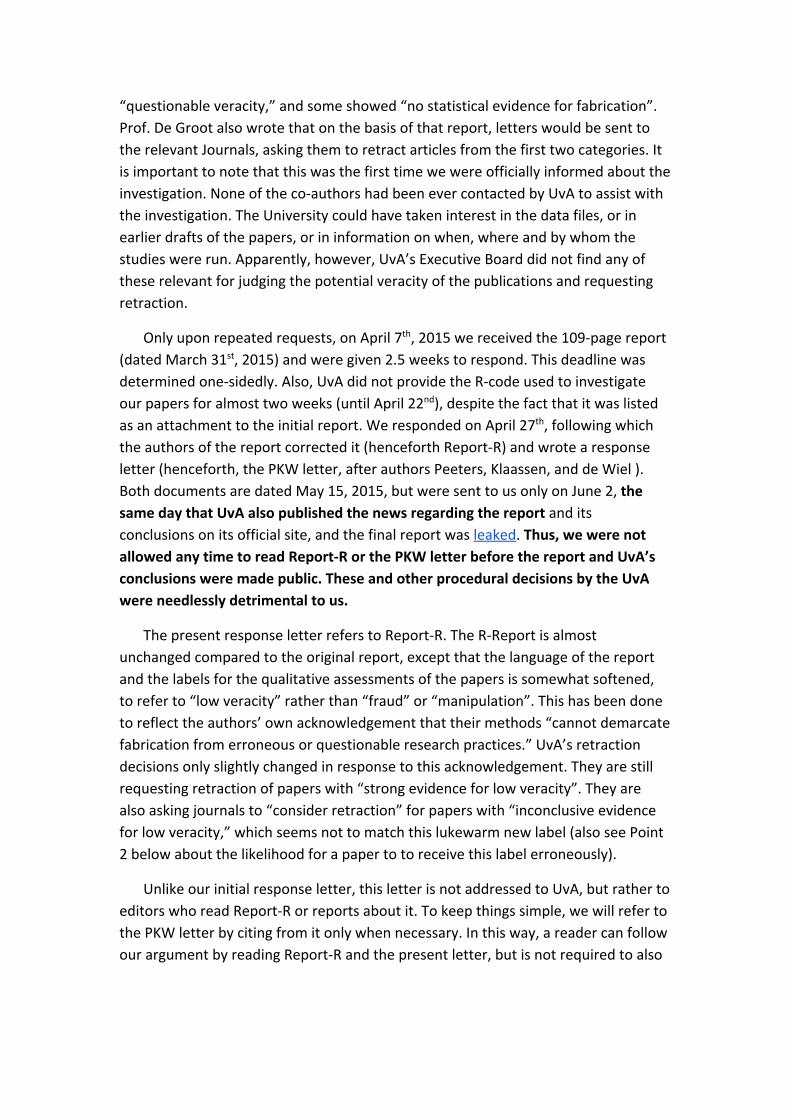
Both documents are dated May 15, 2015, but were sent to us only on June 2, the

same day that UvA also published the news regarding the report and its

conclusions on its official site, and the final report was leaked. Thus, we were not

allowed any time to read Report-R or the PKW letter before the report and UvA’s

conclusions were made public. These and other procedural decisions by the UvA

were needlessly detrimental to us.

The present response letter refers to Report-R. The R-Report is almost

unchanged compared to the original report, except that the language of the report

and the labels for the qualitative assessments of the papers is somewhat softened,

to refer to “low veracity” rather than “fraud” or “manipulation”. This has been done

to reflect the authors’ own acknowledgement that their methods “cannot demarcate

fabrication from erroneous or questionable research practices.” UvA’s retraction

decisions only slightly changed in response to this acknowledgement. They are still

requesting retraction of papers with “strong evidence for low veracity”. They are

also asking journals to “consider retraction” for papers with “inconclusive evidence

for low veracity,” which seems not to match this lukewarm new label (also see Point

2 below about the likelihood for a paper to to receive this label erroneously).

Unlike our initial response letter, this letter is not addressed to UvA, but rather to

editors who read Report-R or reports about it. To keep things simple, we will refer to

the PKW letter by citing from it only when necessary. In this way, a reader can follow

our argument by reading Report-R and the present letter, but is not required to also

https://drive.google.com/file/d/0B5Lm6NdvGIQbamlhVlpESmQwZTA/view

read the original version of the report, our previous response letter, and the PKW

letter.

Because of time pressure, we decided to respond only to findings that concerned

co-authored papers, excluding the by-now-retracted paper Förster and Denzler

(2012, SPPS). We therefore looked at the general introduction of Report-R and at the

sections that concern the following papers:

In the "strong evidence for low veracity" category

Förster and Denzler, 2012, JESP

Förster, Epstude, and Ozelsel, 2009, PSPB

Förster, Liberman, and Shapira, 2009, JEP:G

Liberman and Förster, 2009, JPSP

In the "inconclusive evidence for low veracity" category

Denzler, Förster, and Liberman, 2009, JESP

Förster, Liberman, and Kuschel, 2008, JPSP

Kuschel, Förster, and Denzler, 2010, SPPS

This is not meant to suggest that our criticism does not apply to the other parts

of Report-R. We just did not have sufficient time to carefully examine them. We

would like to elaborate now on points 1-7 above and explain in detail why we think

that UvA’s report is biased, misleading, and flawed.

1. The new method by Klaassen (2015) (the V method) is inherently biased

Report-R heavily relies on a new method for detecting low veracity (Klaassen, 2015),

whose author, Prof. Klaassen, is also one of the authors of Report-R (and its previous

version).

In this method (which we’ll refer to as the V method), a V coefficient is computed

and used as an indicator of data veracity. V is called “evidential value” and is treated

as the belief-updating coefficient in Bayes formula, as in equation (2) in Klaassen

(2015)

For example, according to the V method, when we examine a new study with V = 2,

our posterior odds for fabrication should be double the prior odds. If we now add

another study with V = 3, our confidence in fabrication should triple still. Klaassen,

2015, writes "When a paper contains more than one study based on independent

data, then the evidential values of these studies can and may be combined into an

overall evidential value by multiplication in order to determine the validity of the

whole paper" (p. 10).

The problem is that V is not allowed to be less than unity. This means that there is

nothing that can ever reduce confidence in the hypothesis of "low data veracity".

The V method entails, for example, that the more studies there are in a paper, the

more we should get convinced that the data has low veracity.

Klaassen (2015) writes “we apply the by now standard approach in Forensic

Statistics” (p. 1). We doubt very much, however, that an approach that can only

increase confidence in a defendant’s guilt could be a standard approach in court.

We consulted an expert in Bayesian statistics (s/he preferred not to disclose her

name). S/he found the V method problematic, and noted that quite contrary to the V

method, typical Bayesian methods would allow both upward and downward changes

in one’s confidence in a prior hypothesis.

In their letter, PKW defend the V method by saying that it has been used in the

Stapel and Smeesters cases. As far as we know, however, in these cases there was

other, independent evidence of fraud (e.g., Stapel reported significant effects with

t-test values smaller than 1, in a Smeesters’ data individual scores were distributed

too evenly; see Simonsohn, 2013) and the V method was only supporting other

evidence. In contrast, in our case, labeling the papers in question as having "low

scientific veracity" is almost always based only on V values - the second method for

testing “ultra-linearity” in a set of studies (ΔF combined with the Fisher’s method)

either could not be applied due to a low number of independent studies in the paper

or was applied and did not yield a reason for concern. We do not know what weight

the V method received in the Staple and Smeesters cases (relative to other

evidence), and whether all the experts who examined those cases found the method

useful. As noted before, a statistician we consulted found the method very

problematic.

The authors of Report-R do acknowledge that combining V values becomes

problematic as the number of studies increases (e.g., p. 4) and explain in the PKW

letter that "the conclusions reached in the report are never based on overall

evidential values, but on the (number of) evidential values of individual

samples/sub-experiments that are considered substantial". They nevertheless

proceed to compute overall V's and report them repeatedly in Report-R (e.g., "The

overall V has a lower bound of 9.93", p. 31; "The overall V amounts to 8.77", on p.

66). Why?

2. The criteria for “low veracity” are too inclusive

The following table from Report-R (p. 3) describes the probability of a false alarm,

that is, of erroneously deeming a publication as showing "strong evidence of low

scientific veracity" due to chance (given several assumptions the authors make on

the population and the relations between the samples):

This means that applying the V method across the board would result in erroneously

retracting 1/12-1/19 of all published papers with experimental designs similar to

those examined in Report-R (before taking into account those flagged as exhibiting

“inconclusive” evidence).

In their letter, PKW write "these probabilities are in line with (statistical) standards

for accepting a chance-result as scientific evidence". In fact, these p-values are

higher than is commonly acceptable in science. One would think that in "forensic"

contexts of "fraud detection" the threshold should be, if anything, even higher

(meaning, with lower chance for error).

Report-R says "When there is no strong evidence for low scientific veracity (according to the judgment above), but there are multiple constituent (sub)experiments with a substantial evidential value, then the evidence for low scientific veracity of a publication is considered inconclusive (p.2).” As already mentioned, UvA plans to ask journals to consider retraction of such papers. For example, in Denzler, Förster, and Liberman (2009) there are two Vs that are greater than 6 (Table 14.2) out of 17 V values computed for that paper in Report-R. The probability of obtaining two or more values of 6 or more out of 17 computed values by chance is 0.40. Let us reiterate this figure - 40% chance of type-I error.

Do these thresholds provide good enough reasons to ask journals to retract a paper or consider retraction? Apparently, the Executive Board of the University of Amsterdam thinks so. We are sure that many would disagree.

An anecdotal demonstration of the potential consequences of applying such liberal

standards comes from our examination of a recent publication by Blanken, de Ven,

Zeelenberg, and Meijers (2014, Social Psychology) using the V method. We chose this

paper because it had the appropriate design (three between-subjects conditions)

and was conducted as part of an Open Science replication initiative. It presents three

failures to replicate the moral licensing effect (e.g., Merritt, Effron, & Monin, 2010) .

The whole research process is fully transparent and materials and data are available

online. The three experiments in this paper yield 10 V values, two of which are

higher than 6 (9.02 and 6.18; we thank PKW for correcting a slight error in our earlier

computation). The probability of obtaining two or more V-values of 6 or more out of

10 by chance is 0.19. By the criteria of Report-R, this paper would be classified as

showing “inconclusive evidence of low veracity”. By the standards of UvA’s

Executive Board, which did not seek any confirming evidence to statistical findings

based on the V method, this would require sending a note to the journal asking it

to consider retraction of this failed replication paper. We doubt if many would find

this reasonable.

It is interesting in this context to note that in a different investigation that applied a

variation of the V method (investigation of the Smeesters case) a V = 9 was used as

the threshold. Simply adopting that threshold from previous work in the current

report would dramatically change the conclusions. Of the 20 V values deemed

“substantial” in the papers we consider here, only four have Vs over 9, which would

qualify them as “substantial” with this higher threshold. Accordingly, none of the

papers would have made it to the "strong evidence" category. In addition, three of

the four Vs that are above 9 pertain to control conditions - we elaborate later on

why this might be problematic.

3. Dependence of measurement errors does not necessarily indicate low

veracity

Klaassen (2015) writes: "If authors are fiddling around with data and are fabricating and falsifying data, they tend to underestimate the variation that the data should show due to the randomness within the model. Within the framework of the above ANOVA-regression case, we model this by introducing dependence between the normal random variables εij , which represent the measurement errors" (p. 3). Thus, the argument that underlies the V method is that if fraud tends to create

dependence of measurement errors between independent samples, then any

evidence of such dependence is indicative of fraud. This is a logically invalid

deduction. There are many benign causes that might create dependency between

measurement errors in independent conditions. Here is an example. Suppose you

have a paper-and-pencil experiment with two conditions, A and B, and plan to run 20

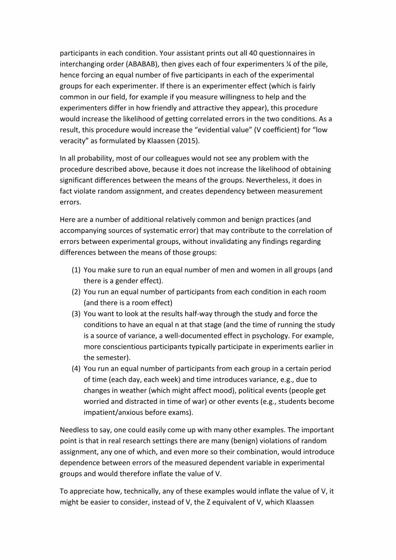
http://www.rsm.nl/fileadmin/Images_NEW/News_Images/2014/Report_Smeesters_follow-up_investigation_committee.final.pdf

http://www.rsm.nl/fileadmin/Images_NEW/News_Images/2014/Report_Smeesters_follow-up_investigation_committee.final.pdf

participants in each condition. Your assistant prints out all 40 questionnaires in

interchanging order (ABABAB), then gives each of four experimenters ¼ of the pile,

hence forcing an equal number of five participants in each of the experimental

groups for each experimenter. If there is an experimenter effect (which is fairly

common in our field, for example if you measure willingness to help and the

experimenters differ in how friendly and attractive they appear), this procedure

would increase the likelihood of getting correlated errors in the two conditions. As a

result, this procedure would increase the “evidential value” (V coefficient) for “low

veracity” as formulated by Klaassen (2015).

In all probability, most of our colleagues would not see any problem with the

procedure described above, because it does not increase the likelihood of obtaining

significant differences between the means of the groups. Nevertheless, it does in

fact violate random assignment, and creates dependency between measurement

errors.

Here are a number of additional relatively common and benign practices (and

accompanying sources of systematic error) that may contribute to the correlation of

errors between experimental groups, without invalidating any findings regarding

differences between the means of those groups:

(1) You make sure to run an equal number of men and women in all groups (and

there is a gender effect).

(2) You run an equal number of participants from each condition in each room

(and there is a room effect)

(3) You want to look at the results half-way through the study and force the

conditions to have an equal n at that stage (and the time of running the study

is a source of variance, a well-documented effect in psychology. For example,

more conscientious participants typically participate in experiments earlier in

the semester).

(4) You run an equal number of participants from each group in a certain period

of time (each day, each week) and time introduces variance, e.g., due to

changes in weather (which might affect mood), political events (people get

worried and distracted in time of war) or other events (e.g., students become

impatient/anxious before exams).

Needless to say, one could easily come up with many other examples. The important

point is that in real research settings there are many (benign) violations of random

assignment, any one of which, and even more so their combination, would introduce

dependence between errors of the measured dependent variable in experimental

groups and would therefore inflate the value of V.

To appreciate how, technically, any of these examples would inflate the value of V, it

might be easier to consider, instead of V, the Z equivalent of V, which Klaassen

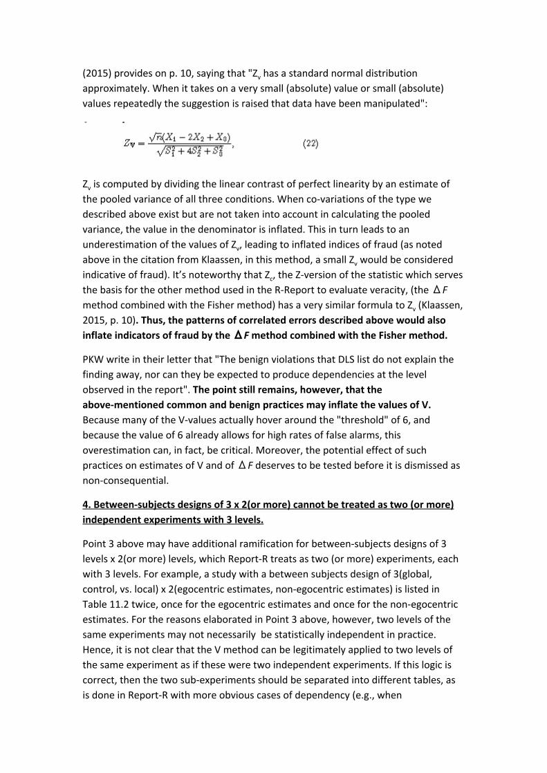
(2015) provides on p. 10, saying that "Zv has a standard normal distribution

approximately. When it takes on a very small (absolute) value or small (absolute)

values repeatedly the suggestion is raised that data have been manipulated":

Zv is computed by dividing the linear contrast of perfect linearity by an estimate of

the pooled variance of all three conditions. When co-variations of the type we

described above exist but are not taken into account in calculating the pooled

variance, the value in the denominator is inflated. This in turn leads to an

underestimation of the values of Zv, leading to inflated indices of fraud (as noted

above in the citation from Klaassen, in this method, a small Zv would be considered

indicative of fraud). It’s noteworthy that Zc, the Z-version of the statistic which serves

the basis for the other method used in the R-Report to evaluate veracity, (the ΔF

method combined with the Fisher method) has a very similar formula to Zv (Klaassen,

2015, p. 10). Thus, the patterns of correlated errors described above would also

inflate indicators of fraud by the ΔF method combined with the Fisher method.

PKW write in their letter that "The benign violations that DLS list do not explain the

finding away, nor can they be expected to produce dependencies at the level

observed in the report". The point still remains, however, that the

above-mentioned common and benign practices may inflate the values of V.

Because many of the V-values actually hover around the "threshold" of 6, and

because the value of 6 already allows for high rates of false alarms, this

overestimation can, in fact, be critical. Moreover, the potential effect of such

practices on estimates of V and of ΔF deserves to be tested before it is dismissed as

non-consequential.

4. Between-subjects designs of 3 x 2(or more) cannot be treated as two (or more)

independent experiments with 3 levels.

Point 3 above may have additional ramification for between-subjects designs of 3

levels x 2(or more) levels, which Report-R treats as two (or more) experiments, each

with 3 levels. For example, a study with a between subjects design of 3(global,

control, vs. local) x 2(egocentric estimates, non-egocentric estimates) is listed in

Table 11.2 twice, once for the egocentric estimates and once for the non-egocentric

estimates. For the reasons elaborated in Point 3 above, however, two levels of the

same experiments may not necessarily be statistically independent in practice.

Hence, it is not clear that the V method can be legitimately applied to two levels of

the same experiment as if these were two independent experiments. If this logic is

correct, then the two sub-experiments should be separated into different tables, as

is done in Report-R with more obvious cases of dependency (e.g., when

within-subjects factors cross the 3-levels between-subject factor). If potentially

dependent results are separated into two tables, all the indexes of “low veracity”

would go down: the number of “substantial” V values in each of these two tables

would not be added to each other and the estimates of both ΔF and overall V value

would be lower.

5. Applying the V and the ΔF methods to control measures is wrong

The authors apply the V method both to cases in which significant differences

between the means of the three groups were predicted and found, and to cases in

which such differences were neither predicted nor found. This is wrong. If we do not

predict any differences between means and then indeed get three means that are

not significantly different from each other, then a linear pattern (e.g., X1 = 5, X2 = 6, X3

= 7) should not be any more “suspicious” than a non-linear pattern (e.g., X1 = 6, X2 =

7, X3 = 5). Yet, both the K method and the ΔF method would render the former

pattern more suspicious than the latter (see, for example, equation for Zv above. The

numerator for Zc is the same, see Klaassen, 2015, p10, equations 22 and 23).

For such control conditions, the authors should have used the following two

contrasts, which represent equality of means:

(a) X1 – X2 + 0X3 = 0; and X1 + 0X2 – X3 = 0

instead of the linear contrast that they used in the numerator of their indicators:

(b) X1– 2X2 + X3 = 0.

Some of the V values in Report-R are clearly over-estimated due to using the

wrong contrast (b). Consider, for example, the three means (4.41, 4.53, 4.64) and

their corresponding standard deviations (0.40, 0.45, 0.49), which yield a V value of

18.0583 (Table 9.3, p. 55). Förster, Liberman, and Kuschel (2008), the authors of this

paper, did not predict these means to differ from each other, and indeed found no

significant differences between them. Note, also, that the means are not "too good

to be true" in the sense that they are not too close to the theoretically-predicted

pattern X1 = X2 = X3. In fact, the means differ from each other considerably, by 0.24 -

0.3 SDs. We think that they would not have been flagged at all if the authors applied

the proper contrasts (a) instead of (b). Ten out the 20 “substantial” V values in the

relevant papers pertain to control conditions and might have been inflated.

It is possible, of course, that values that are not flagged now would be flagged

once the proper contrast is used. Regardless of the outcome, however, the right

contrast should be used for control conditions.

6. The V-value is sensitive to rounding-of-values

The V value appears to be sensitive to very small variations in the values of the cell

means. For example, in Table 8.2, Exp5a the means (0.25, 0.13, 0.02) yield V = 7.28.

If, however, the means are changed slightly (within the boundaries of rounding!) to

(0.254, 0.125, 0.02) with the same SDs, we now get V = 3.09. To give another

example from the same table, in Exp5b the means 0.29, 0.14, 0.00 give V = 7.24. If

the means are changed slightly to 0.29, 0.136, 0.004 (note again that these numbers,

if rounded, would be identical to the original ones) and with the same SDs we get V =

3.34. This sensitivity to rounding does not seem like a desirable feature for a metric

used to detect fraud.

In their letter, PKW note that they can as easily find a perturbation of means within

the boundaries of rounding that actually increases V values. We agree. We think that

all the values of means and standard deviations that go into computing V and ΔF

should be allowed to perturbate within the boundaries of rounding. Doing that

would more correctly portray what these values really mean. For example, a value of

0.55 does not represent 0.55000 but rather a range between 0.545001 and

0.554999. The authors should use (as they do now) the lower boundary of these

post-perturbation estimations.

In their letter, PKW write "As the report contains many evidential values, we can safely assume that instances in which an evidential value would fall below the threshold of 6 under recomputation with higher precision summary statistics, will be balanced by instances in which the evidential value would jump above the threshold for considering an evidential value substantial under such re-computation." We are not convinced that this is indeed the case. It is easy to imagine a situation in which reducing precision (or adding noise) would actually increase the overall number of “substantial” V values. For example, consider a case in which there are 10 values of V = 8 and 90 values of V = 4. We introduce noise by adding 3 to half the values and subtracting 3 from the other half (half of each category). That would give us five Vs of 8 + 3 = 11, five Vs of 8 - 3 = 5, 45 Vs of 4 + 3 = 7 and 45 Vs of 4 - 3 = 1. We now end up having 50 Vs higher than six, compared to the 10 that we had before adding noise. 7. Examining individual papers

We are now in a position to look at the evidence for any “low scientific veracity“ in

each of the co-authored papers in Report-R (as noted above, we exclude the

by-now-retracted SPPS 2012 paper). For each paper, we present the means, SDs and

Vs for those V values that were deemed “substantial“ in the report. We also report

its status in regards to the results of the ΔF paired with Fisher’s method.

In the "strong evidence for low veracity" category

7.1 Förster and Denzler (2012, JESP) - JF.D12.JESP

Overall number of computed V values: 12

Study Means SDs V

1. study1.ex1.liking 1.65 1.95 2.20 3.0 1.40 1.44 7.5437–11.8122

2. study2.ex1.liking 2.14 2.30 2.48 1.7 1.58 1.95 8.1808–26.0208

3. study1.ex3.liking -2.35 -0.45 1.55 2.43 1.85 2.09 6.6032–6.6669

4. study1.ex3.reac 4733 5056 5361 375 491 529 8.8874

ΔF paired with Fisher’s method: Number of independent studies too low to apply

The first two rows pertain to null results, thus values are inflated due to using the

wrong contrast (Point 5).

Lines 1, 3 and 4 pertain to the same participants (they are different DVs in the same

condition or different conditions in a within-subjects design). They are not

independent.

We do not think that these results convey “strong“ (or any) evidence of “low

scientific veracity“.

7.2 Förster, Epstude, and Özelsel (2009, PSPB) - JF.EO09.PSPB


Study Means SDs V

1. study2.ana 0.80 1.5 2.25 1.06 0.95 1.25 6.6866–6.8333

2. study2.gl 26.3 33.4 40.1 8.87 8.58 9.61 7.3405


These two V values pertain to the same participants (they are different DVs in a

within-subjects design). They are not independent.



7.3 Förster, Liberman, and Shapira (2009, JEP:G) - JF.LS09.JEPG


Study Means SDs V

1. exp5a 0.02 0.13 0.25 0.23 0.22 0.20 7.2848

2. exp5b 0.00 0.14 0.29 0.19 0.18 0.18 7.2405

3. exp4a.PT 6.91 7.03 7.12 0.55 0.51 0.65 6.5389–7.7784

4. exp4b.Typ 6.66 6.71 6.75 0.31 0.22 0.21 7.6776–10.1341

5. exp1b.locER 0.56 1.00 1.38 0.89 0.89 1.31 6.0519

ΔF paired with Fisher’s method: “Does not give immediate reason for concern”

The V values in rows 1 and 2 decrease dramatically if the values of means and

standard deviations are changed slightly, within the boundaries of rounding (Point

6).

The V values in rows 3 and 4 pertain to null results, and are inflated due to using the

wrong contrast (Point 5).

The V value in row 5 barely crossed the (already fairly low) threshold of 6 (Point 2).

Please also note that V for the pooled results the authors report for Experiment 4a,

which they deem “substantive” (p. 51) and factor into their final conclusion (p. 52)

actually does not cross their own threshold (V = 4.12).



7.4 Liberman and Förster (2009, JPSP) - L.JF09.JPSP


ΔF paired with Fisher’s method: “Both an extreme and a moderate result are

obtained”

This is the only article in the set of articles we examined for which the ΔF test of

excessive linearity showed any “reason for concern“. We thus present here the full

results of all the V and ΔF tests for all the studies in the article. The tables are

copied from the Report-R.

The bottom half of Table 11.2 pertains to null results, and many of its values

probably show excessive linearity due to using the wrong contrast (Point 5).

In addition, there might be some dependency between the different conditions of

the same study (Point 4). Splitting Table 11.2 to two would have considerably

reduced indexes of excessive linearity by the ΔF test.

Only two V values in this set of 18 values cross the (already fairly low) threshold of 6,

one of them barely so (Point 2).

We do not believe that the results in this study convey “strong“ (or any) evidence of

“low scientific veracity“.

In the "inconclusive evidence for low veracity" category

7.5 Förster, Liberman, and Kuschel (2008, JPSP) - JF.LK08.JPSP

Overall number of computed V values: 27 (20 of them appear in tables, 7 more are

computed for “pooled results” and are presented only in figures).

Study Means SDs V

1. exp1.RU.np 4.41 4.53 4.64 0.40 0.45 0.49 18.0583

ΔF paired with Fisher’s method: “Does not give immediate reason for concern”

This single V value pertains to null results, and is thus inflated due to using the wrong

contrast (Point 5).

Why is this paper even included in the “suspects“ list? Let us cite Report-R : “While

the Fisher test does not give immediate reason for concern, the evidential value for

at least 1 (sub)experiment is substantial, implying the presence of a dependence

structure between test persons. This high evidential value for exp1.RU.np in

conjunction with the high evidential values for the pooled results of Experiment 3

(see Figure 9.5 and the last sentence of Section 9.2.4) deems the conclusion that the

evidence for low scientific veracity of this publication is inconclusive” (p.58).

By “pooled results” the authors are referring to sometimes employing their method

in factorial designs on the marginal means (and associated SDs, for the main

experimental factor) in addition to the cell means (and associated SDs, for the simple

effect of the main experimental factor at each level of a secondary factor). In the

case of this paper, the authors report: “Using grand means over the reported cell

means of the main experimental factor and using the corresponding average

variance in order to obtain pooled standard deviations the subjective scale and the

objective scale would sort substantive evidential values with lower-bounds of 5.05

and 18.13, respectively.” (p. 57)

The means and standard deviations of individual “pooled results“ are not presented

in tables, but rather only in Figure 9.5. There are seven pooled results in that figure.

The V value of only one of them crosses the threshold of 6. Eye balling this figure for

seemingly linear pattern, this high V of 18.13 clearly pertains to a flat (horizontal)

line, and thus might be inflated due to using the wrong contrast (Point 5). Perhaps

more importantly, Report-R never explains when and how it uses “pooling“. Are all

the results “pooled“ in all possible combinations? Obviously not.

In any event, the probability of obtaining by chance at least two “substantive” V

values among 27 computed V values is 65%.

We mentioned this study in our initial letter to the authors. In their response PKW

said „We clearly state on page 2 that we apply the guidelines with care, i.e., we do not

apply them blindly.” We agree. They certainly do not apply the criteria blindly.

We do not think that the results in this paper convey “inconclusive“ (or any)

evidence of “low scientific veracity“.

7.6 Kuschel, Förster, & Denzler (2010, SPPS) - K.JF.D10.SPPS


Study Means SDs V

1. Exp3.correctReject 4 4.60 4.80 5.00 0.83 0.41 0.00 116.6748–NaN


Once again, we need to resort to Report-R to understand why this study was listed as

showing indication of “low veracity”: “...While according to a strict application of the

criterion of Section 1.4 this publication should be classified as containing no evidence

for low veracity, we conclude, on the basis of the peculiarity of the results pertaining

to Exp3.correctReject, that the evidence for low veracity of this publication has to be

classified as inconclusive.” (p. 78).

This “peculiarity of the results“ is a standard deviation of zero in one of the

conditions of Study 3. In this study, participants classified metaphors and literal

sentences as “metaphors” versus “non metaphors”. In one of the conditions, each of

the 15 participants correctly classified five out of five “non-metaphors” as

“non-metaphors”. This information is in the paper. To us, this result sounds entirely

plausible (note also that the main DV of interest was reaction time, not error-rate).

We do not think that the results in this study feature “inconclusive“ (or any)

evidence of “low scientific veracity“.

7.7 Denzler, Förster, and Liberman (2009, JESP) - D.JF.L09.JESP


Study Means SDs V

1. exp1.WU.NS.B1 704 710 711 100 112 88 6.2716–8.1405

2. exp1.WU.S.B3 699 713 723 84 61 92 6.8163

3. exp2.BA 4.13 4.61 5.11 0.57 0.75 0.5 3.8421–12.3772


The V values in Lines 1 and 2 pertain to flat lines, and are very likely inflated due to

using the wrong contrast (Point 5).

We are not quite sure why the V value in row 3 was deemed “substantial“. Report-R

clearly says that the relevant V value for judging “veracity” is the lower bound one .

For some reason, the authors chose to deviate from their own rule in this particular

case „The upper-bound for the evidential value may be termed substantial

(12.3772)”. We are not sure why.

We do not think that the results in this study convey “inconclusive“ (or any) evidence

of “low scientific veracity“.

Summary

We found the report by UvA on the case of Jens Forster misleading and biased. We

surmise that it does not present reliable evidence for “low scientific veracity”.

References

● Blanken, I., van de Ven, N., Zeelenberg, M., & Meijers, M. H. (2014). Three attempts to replicate the moral licensing effect. Social Psychology, 45(3), 232-238.

● Denzler, M., Forster, J., and Liberman, N. (2009). How goal-fulllment decreases aggression. Journal of Experimental Social Psychology, 45: 90-100.

● Forster, J. and Denzler, M. (2012). When any worx looks typical to you: Global relative to local processing increases prototypicality and liking. Journal of Experimental Social Psychology, 48: 416-419.

● Forster, J., Epstude, K., and Ozelsel, A. (2009). Why love has wings and sex has not: How reminders of love and sex in uence creative and analytic thinking. Personality and Social Psychology Bulletin, 35: 1479-1491.

● Forster, J., Liberman, N., and Kuschel, S. (2008). The effect of global versus local processing styles on assimilation versus contrast in social judgment. Journal of Personality and Social Psychology, 94: 579-599.

● Forster, J., Liberman, N., and Shapira, O. (2009). Preparing for novel versus familiar events: Shifts in global and local processing. Journal of Experimental Psychology: General, 138: 383-399.

● Klaassen, C. A. J. (2015). Evidential value in ANOVA-regression results in scientific integrity studies. arXiv:1405.4540v2 [stat.ME].

● Kuschel, S., Forster, J., and Denzler, M. (2010). Going beyond information given: How approach versus avoidance cues in uence access to higher order information. Social Psychological and Personality Science, 1: 4-11.

● Liberman, N. and Forster, J. (2009). Distancing from experienced self: How global-versus-local perception affects estimation of psychological distance. Journal of Personality and Social Psychology, 97: 203-216.

● Merritt, A. C., Effron, D. A., & Monin, B. (2010). Moral self-licensing: When being good frees us to be bad. Social and personality psychology compass,4(5), 344-357.

nira liberman, school of psychological sciences, tel · pdf file06.06.2015 · nira...

Documents