nih public access abstract metabolomics data methods …xbw/research/nihms656480.pdf · statistical...

Statistical Analysis and Modeling of Mass Spectrometry-Based Metabolomics Data

Bowei Xi, Haiwei Gu, Hamid Baniasadi, and Daniel Raftery

Abstract

Multivariate statistical techniques are used extensively in metabolomics studies, ranging from

biomarker selection to model building and validation. Two model independent variable selection

techniques, principal component analysis and two sample t-tests are discussed in this chapter, as

well as classification and regression models and model related variable selection techniques,

including partial least squares, logistic regression, support vector machine, and random forest.

Model evaluation and validation methods, such as leave-one-out cross-validation, Monte Carlo

cross-validation, and receiver operating characteristic analysis, are introduced with an emphasis to

avoid over-fitting the data. The advantages and the limitations of the statistical techniques are also

discussed in this chapter.

Keywords

Metabolomics; Mass spectrometry; Multivariate statistics; Classification

1 Introduction

In many typical metabolomics studies, a large number of metabolite molecular signatures

are measured quantitatively from biofluids, such as blood and urine, from either animals or

humans. Metabolomics data provide important information about biomarkers and metabolic

pathways related to disease, gender, diet, etc. Since metabolites are the downstream products

of genes and gene expression, and thus are very sensitive to various biological states, they

can potentially be more readily used for early disease detection than other molecular

information, as well as for providing contemporaneous information for a variety of other

studies. Liquid chromatography-mass spectrometry (LC-MS) and gas chromatography-mass

spectrometry (GC-MS) are analytical techniques that have often been used in metabolomics

studies to generate the high content data. Another important component is to apply

multivariate statistical techniques to analyze the MS-based metabolomics data.

There are multiple statistical techniques available for every data analysis task, including

many powerful classification and regression models, and multiple model validation

methods. Biomarker selection can be either an independent step or a byproduct of a model.

Various statistical techniques can be combined in a proper way to identify potential

biomarkers and demonstrate how useful the selected biomarkers are. This article discusses

© Springer Science+Business Media New York 2014

NIH Public AccessAuthor ManuscriptMethods Mol Biol. Author manuscript; available in PMC 2015 February 06.

Published in final edited form as:Methods Mol Biol. 2014 ; 1198: 333–353. doi:10.1007/978-1-4939-1258-2_22.

NIH

-PA

Author M

anuscriptN

IH-P

A A

uthor Manuscript

NIH

-PA

Author M

anuscript

four models, partial least squares, logistic regression, support vector machine, and random

forest, and the related model based variable selection techniques. Two model independent

variable selection techniques, principal component analysis and two sample t-tests are also

introduced.

A key issue for metabolomics studies is to avoid over-fitting the data. Because of the large

number of metabolites and the relatively small sample size, a complex model can over-

utilize (over-fit) the data specific information and show very good performance, but that

good result is useless if it cannot be duplicated using a new set of test data. Proper model

evaluation and validation is therefore a necessary step to understand the true performance of

a model and the potential biomarkers. Cross-validation, Monte Carlo cross-validation

(MCCV), and receiver operating characteristic (ROC) analysis are discussed in this article.

2 Data Processing and Metabolite Identification

2.1 Data Extraction

Liquid chromatography (LC) and gas chromatography (GC) are the two most commonly

used separation methods prior to mass spectrometric (MS) analysis. Generally, the

instrument manufacturer will provide software to process raw data and generate a list of ion

intensities/areas for detected peaks after peak picking, peak de-convolution, peak alignment,

etc. For example, Agilent’s MassHunter Qualitative Analysis software can be used for peak

identification and Agilent’s Mass Profiler Professional software also has functions for

metabolite identification. The compound identification can be assisted by various databases

containing the information of retention time, accurate mass, and tandem mass spectrometry.

The NIST MS database [1] is often used for the data from electron ionization (EI) that is

typically utilized in GC-MS. The Metlin Database [2] is especially suitable for the

identification of metabolites in LC-MS data sets as it contains the MS/MS spectra of more

than ten thousand standard compounds.

2.2 Preprocessing

Prior to the actual multivariate statistical analysis, some steps are necessary to be performed

on spectral data in order to obtain meaningful information. Useful preprocessing methods

mainly include normalization, mean-centering, and scaling. These steps can be used

individually or in combination. It should be noted that the reproducibility of MS can be a

concern (i.e., operated without internal standards for each compound of interest), and thus

quality controls are normally included in experiments to compensate instrument drift.

2.2.1 Normalization—For biofluids, especially urine samples, the concentrations of

metabolites are highly dependent on factors that are generally not of interest to

metabolomics studies, such as the amount of consumed water. Normalization is an important

and effective method to exclude or reduce the unwanted overall variations in spectral data.

There are three commonly used approaches to normalize data sets in metabolomics. The first

approach is total signal normalization, which calculates the total intensity of the whole

spectrum or total ion count and then sets it to a constant value. The second method is vector

length normalization. Each spectrum containing many variables can be regarded as a point

Xi et al.

Methods Mol Biol. Author manuscript; available in PMC 2015 February 06.

NIH

-PA

Author M

anuscriptN

IH-P

A A

uthor Manuscript

NIH

-PA

Author M

anuscript

in a high dimensional space. The vector length normalization sets the Euclidean distance in

the multidimensional space to be constant. The last approach is to divide the whole spectrum

by a certain peak intensity (typically the largest peak). In the medical community, creatinine

is often used as an intensity reference for urine samples. This is due to the underlying

assumption of constant excretion of creatinine into urine, which generally holds except for

some diseases that affect kidney function. Creatinine levels in urine also show a slight age

dependence [3].

2.2.2 Mean-Centering—Mean-centering is often carried out to center the data distribution

at the origin in the multidimensional space. In a typical data matrix used for multivariate

statistical analysis, each row represents a different sample while the metabolite identities,

m/z, or peak variables are aligned into specific columns. Mean-centering is performed by

subtracting the mean value of each peak (column) from the corresponding variable in each

sample (row).

2.2.3 Scaling—Multivariate statistical analysis tends to focus on metabolites with high

intensities. However, low-concentration metabolites may also play important roles in the

biological processes. Scaling is often used in metabolomics to change the emphasis from

metabolites with high concentrations to those with moderate or small abundances. Variance

scaling calculates the standard deviation of each variable (column) and then divides each

column by this value. The combination of mean-centering and variance scaling is termed

auto-scaling. Auto-scaling sets all variables to unit variance. Auto-scaling is highly

recommended when variables have different units. Nevertheless, one drawback of this

operation is that it may increase the contribution of noise variables to the analysis. To

minimize the undesirable noise effect, Pareto scaling, which uses the square root of the

standard deviation as the scaling parameter, can be used. Pareto scaling falls in between no-

scaling and auto-scaling, and thus has become more popular in metabolomics to avoid over-

manipulating the data. In addition, log scaling can also be used to reduce the effect of large

peaks in data analysis and make the data more normal-distributed (many statistical methods

were developed assuming that the data follow a normal distribution). However, a drawback

of log scaling is that it is unable to deal with zero/negative values.

3 Variable Selection (See Note 1)

After the metabolomics data are created and organized into matrix format, multivariate

statistical analysis is performed to identify bio-marker candidates and to examine how well

the different groups in the data set are separated using those biomarker candidates through a

classification model. Variable selection is a step to identify relevant and putative

biomarkers. Variable selection can be performed prior to building a classification model or

as a byproduct of a classification model. GC-MS data and LC-MS data typically contain

1It is interesting to note that different variable selection procedures may select different sets of biomarkers. The reason is that they conduct variable selection from different perspectives. Model based variable selection procedures take into account the joint effect of all metabolites within a specific model framework. PCA utilizes the correlation structure of metabolites. The t-test examines the mean values of the two groups. Hence, it is not surprising that they return different results. Different sets of selected variables are all potential candidates for an effective classification model. A variable selection step may employ one or several statistical techniques to select potential biomarkers and combine the results if multiple techniques are used. Prior knowledge such as previous studies about a disease and metabolic pathways must also be considered along with statistical analysis in variable selection.

Xi et al.


NIH

-PA

Author M

anuscriptN

IH-P

A A

uthor Manuscript

NIH

-PA

Author M

anuscript

signals from several hundred to over a thousand metabolites. Their peak intensities are

collected for every sample and become candidates for variable selection. The number of

candidate variables is typically relatively large compared with the sample size, and

sometimes much larger than the sample size. Because many of the candidate variables are

not related to the study, variable selection is a crucial step for metabolomics data analysis

and modeling.

There are multiple popular variable selection techniques with slightly different objectives.

Some variable selection techniques directly identify relevant metabolites, while other

techniques serve as a screening process to eliminate irrelevant metabolites. However, none

of the techniques can claim that its results are consistently better than others. Furthermore,

biological and analytical knowledge must be combined with statistical techniques for

biomarker selection; e.g., certain metabolites have been previously shown to be related to a

disease. Metabolic pathways also provide important information about disease related

biomarkers.

In this section, we discuss principal component analysis (PCA) and two sample t-tests.

Neither of these techniques depends on the choice of the classification model. Model based

variable selection procedures through penalized logistic regression and partial least squares

discriminant analysis (PLS-DA) are discussed in Subheading 4.

3.1 Principal Component Analysis

PCA can be described as follows. Assume there are p metabolites, X=(X1, X2,…, Xp), with a

variance-covariance matrix Σ. Let (λk, ek), k =1,2,…, p, be the eigenvalue and eigenvector

pairs of Σ. Arrange the eigenvalues such that λ1 ≥ λ2 ≥ … ≥ λp. The kth principal component

(PC) is Wk = ekTX, and its variance is equal to λk. ek is the loading of the kth PC. The

principal components, W1, W2,…, Wp, are formed by an orthogonal transformation of the

metabolites X. The first PC W1 follows the direction of the maximum variance. The kth PC,

Wk, follows the direction of the largest variance in the subspace that is perpendicular to the

first k−1 PCs. The PCs thus form another set of orthogonal axes in the multidimensional

space. The sum of the variances of the PCs equals to the sum of the variances of the

metabolites X.

When the metabolites X are correlated, some smaller eigenvalues, λK+1,…, λp, are close to 0.

Hence, the first k PCs, W1,…, Wk, can capture a large portion of the total variance in the

original data. In subsequent analysis, the metabolites X can be replaced by the first k PCs,

W1,…, Wk, without much loss of information [4].

It is a common practice to keep the first two or three PCs and examine the score plots. There

is no guarantee that the different groups will be well-separated on the PC score plots, since

PCA is not designed for classification purposes. However, when the groups are well

separated, which happens in many studies, the metabolites that have large loadings in the

first two or three PCs can be selected as potential biomarkers. PCA thus serves for a useful

variable selection purpose (e.g., see refs. 5–8).

Xi et al.


NIH

-PA

Author M

anuscriptN

IH-P

A A

uthor Manuscript

NIH

-PA

Author M

anuscript

PCA can be applied to the scaled data instead of the original data. Several scaling options

are discussed in Subheading 2. PCs from the unscaled data are dominated by a few

metabolites with the largest peak intensities. Scaling (partially) solves this problem, but the

PC scores and loadings from the scaled data are more difficult to interpret. Also notice that

there is no apparent relationship between the PC scores and loadings from the original and

the scaled data.

In a breast cancer study [9], PCA was applied to the mean-centered DART-MS spectra of 57

serum samples. There were 30 healthy controls and 27 breast cancer patients. Figure 1

shows the PC score plot and the PC loading plot. DART-MS PC scores alone cannot

separate the two groups, providing a counter example to show that PCA is not designed for

classification. Hence, a hybrid method, the principal component directed partial least

squares model was proposed [9] to combine the NMR and DART-MS spectra. Using both

spectra the proposed classification model then successfully separated the two groups and

identified breast cancer related biomarker candidates.

3.2 Two Sample T-Tests and Multiple Comparisons

Two sample t-tests are used to show which metabolites have the power to differentiate the

different groups in the data set (e.g., ref. 8). There are a variety of t-tests: the original

Student’s t-test assumes normally distributed data with equal group variances; Welch’s t-test

allows for unequal variances; the Wilcoxon-Mann-Whitney test uses a ranked set of values

and thus allows for non-normally distributed data sets; and several other variants. The two

sample t-test is applied to one metabolite at a time (i.e., a univariate analysis) to determine

whether the mean values of the two groups are different. The null hypothesis for the test is

H0 : μgroup1 = μgroup2, and the alternative hypothesis is Ha : μgroup1 ≠ μgroup2. If the p-value

for the test is smaller than a cutoff value, typically 0.05, the null hypothesis is rejected. If the

p-value is large, there is no significant difference between the mean values for the two

groups, indicating the metabolite has little power to separate them. On the other hand, a

small p-value does not guarantee that the metabolite has sufficient power to separate the two

groups in classification. Even if the mean values are different for the two groups, the

samples from the two groups may still show large overlap. Hence the metabolites with small

p-values must be further evaluated when building a classification model.

The 0.05 cutoff value is often used when the t-test for a metabolite is examined individually,

without considering the tests for other metabolites. A multiple comparison procedure can be

employed, in which a smaller cutoff value is used, to control the overall error caused by

using all the t-tests together. Because of the large number of metabolites in the data, simple

multiple comparison procedures such as the Bonferroni correction are too conservative and

do not work well [10]; they set a cutoff value that is too close to 0 as the number of tests

becomes large.

Multiple comparison procedures have a history dating back to the 1950s, and there are now

many proposed procedures. The Benjamini–Hochberg procedure [11] controls the false

discovery rate at level α (e.g., α = 0.05) as follows. Assume there are m metabolites being

examined. It is a step-up procedure:

Xi et al.


NIH

-PA

Author M

anuscriptN

IH-P

A A

uthor Manuscript

NIH

-PA

Author M

anuscript

1. Order the p-values as p(1) ≤ p(2) ≤ … ≤ p(m);

2.Find the largest k such that , and reject the null hypotheses for the

corresponding tests.

Additional methods for false discovery rate are also commonly used, such as the q-value

[12] and the Benjamini–Hochberg–Yekutieli procedure under dependence assumptions [13].

However, since the metabolites with small p-values are further examined when building a

classification model, and the final decision regarding which biomarkers are related to the

study is not based on the t-tests alone, a simple 0.05 cutoff can often be used instead of a

multiple comparison procedure [14].

3.3 Example Analysis

As an example, we apply several of the statistical techniques described in this chapter to a

liver cancer LC-MS dataset [15] for demonstration purposes. Hepatitis C virus (HCV)

infection of the liver is a major risk factor for the development of hepatocellular carcinoma

(HCC). Serum samples (30 HCC patients with underlying HCV and 22 HCV patients

without HCC) were obtained from the Indiana University/Lilly tissue bank, and targeted LC-

MS/MS data were obtained and used in the study. 73 targeted metabolites were detected in

both the HCC patients and the HCV patients, of which 39 were detected in negative

ionization mode and 34 were detected in positive ionization mode. 16 of the 73 metabolites

had p-values less than 0.05, as shown in Table 1. The four metabolites with the smallest p-

values were used in constructing classification models later. Despite the small number of

samples available, this data set is useful to provide examples of the different analysis

approaches.

4 Classification Models

Classification models can be constructed in a variety of ways, such as using all the

metabolite signals in the data, followed by the selection of biomarkers from the model

results. Another option is to employ variable selection as the first step, where several

metabolites are identified as either potentially correlated with the group differences, or

having little power to separate the groups (after which they could then be eliminated).

Following the variable selection step, classification models can be constructed based on the

combined pool of candidate metabolites, which will be further examined in this process. The

final classification model may use either all the candidate variables or just a subset of them

for the best classification performance. Because the sample size is often not large, the final

classification model needs to be validated to avoid over-fitting the data.

Classification models utilize two matrices, an X matrix for the metabolite peak intensities

and a Y matrix for the class labels. There are multiple powerful classification methods and

numerous variations of them. This section introduces several popular methods used in the

metabolomics field: PLS-DA, logistic regression, support vector machine (SVM), and

random forest.

Xi et al.


NIH

-PA

Author M

anuscriptN

IH-P

A A

uthor Manuscript

NIH

-PA

Author M

anuscript

4.1 Partial Least Squares Discriminant Analysis

The selection of axes in general PLS models is based on the regression of X against Y, and

thus PLS can express the maximum variance from both X and Y matrices. As a bilinear

model, PLS fits the data and recasts them as score plots, loading plots, and weight plots.

While loading plots summarize the observations in the X matrix, weight plots express the

correlation between the X matrix and score values. The PLS score plot is generated by

projection of the original spectra onto the new coordinate system. Each orthogonal axis in

the score plot is called a latent variable (LV), similar to a PC in PCA. Corresponding

loadings or weights contain information about the importance of each variable in the model.

For classification purposes, Y is a dummy matrix, i.e., 0s and 1s are often used to represent

the group assignment of samples. With such a Y matrix, PLS is referred to PLS-DA. PLS-

DA is a typical supervised method in that it requires the class membership knowledge of

biological specimens. If PCA is not successful in showing the subtle difference among the

sample groups, PLS-DA modeling can be used to maximize the separation among the

sample groups and target putative biomarkers for metabolomics studies. Notably, variable

importance in projection (VIP) values estimate the importance of each variable in the

projection used in a PLS model and are often used for variable selection.

4.1.1 PLS Analysis Example—A PLS-DA model was developed for the liver cancer

data based on four metabolites with the lowest p-values [15]. Figure 2 shows the three

dimensional PLS-DA score plot and the predicted Y values of the liver cancer data. The two

groups, HCC and HCV are well separated, with only a small overlap. Figure 3 shows the

PLS-DA VIP plot of the liver cancer data, indicating the relative contributions of each of the

four metabolites to the overall model.

A challenge in using multivariate supervised methods is that they may over-fit the data and

give too optimistic results. A strict cross-validation step is necessary before drawing a

reliable conclusion. Generally speaking, there are “internal” and “external” cross-

validations. The leave-one-out cross-validation procedure, a typical internal cross-validation

approach, is commonly employed to select the number of LVs and to find an optimal PLS-

DA model. From the internal cross-validation step, the root-mean-square error of cross-

validation (RMSECV) curve is created, representing the accuracy of prediction, and is used

to choose the number of LVs. Afterwards, external cross-validation is employed to measure

the model performance. There are several options for external cross-validation, such as

splitting data into two halves, k-fold cross-validation, and MCCV, as described in

Subheading 5. If a test set of samples acquired from one or more different locations is

available, it offers a more accurate validation result for a set of putative biomarkers.

4.1.2 Orthogonal Signal Correction—It is well known that metabolic profiles of

biological samples provide a fingerprint of endogenous markers that can be correlated to a

number of factors such as disease, diet, toxicity, medication intake, etc. Because these

factors can cause significant changes in metabolic profiles, the analysis of MS data is often

aided by the use of statistical methods that can de-convolute the metabolite contributions

from specific factors. For this purpose, orthogonal signal correction (OSC) was developed

Xi et al.


NIH

-PA

Author M

anuscriptN

IH-P

A A

uthor Manuscript

NIH

-PA

Author M

anuscript

and introduced to the metabolomics field to remove chemical and thermal noise, as well as

other variables that are not of interest to the study [16]. OSC is a PLS based data filtering

technique. There are two matrices involved, the X matrix (spectral data) and the Y matrix

(variables of interest). In the OSC step, the structure in the X matrix that is mathematically

orthogonal to the Y matrix data is subtracted. Hence the corrected X matrix contains the Y

matrix related variation. A PLS model based on the corrected X matrix now focuses more on

the variables of interest.

4.2 Logistic Regression

The standard logistic regression model predicts the probabilities of a sample being a member

of either of two groups for a set of metabolite peak intensities. Mathematically, let p(1|X)

and p(2|X) be the probabilities that a sample belongs to group 1 and 2, respectively, given

the metabolite peak intensities X (note that p(1|X)+p(2|X) = 1). The probabilities are modeled

as a function of X as follows in Eq. (1):

(1)

The response variable of the i-th sample for the logistic regression model, Yi, is binary, 1 or

0, corresponding to the two groups. The coefficients in the above model are estimated by

maximizing the log likelihood function Σ(Yilog(p(1|Xi))+(1−Yi) log(p(2|Xi))), where Xi

contains the metabolite peak intensities of the i-th sample. With the estimated coefficients

from a training set of data, the probabilities can be computed for a test set. A test sample is

classified into a group with a probability larger than 0.5. As a classification model, standard

logistic regression can be used in place of PLS-DA (e.g., ref. 17).

There is one major difference between the two models. PLS-DA can be constructed using all

the metabolites in the data, without any prior variable selection step, whereas the standard

logistic regression model has difficulty handling a large number of variables. Typically,

therefore, variable selection is performed before fitting a standard logistic regression model

[18]. The standard logistic regression model is then constructed using the selected

metabolites from the previous variable selection step. In general PLS-DA can handle high

dimensional, correlated data better than logistic regression, which can become an issue for

highly correlated metabolites.

4.2.1 Penalized Logistic Regression—Penalized logistic regression, a variant of the

logistic regression model [19], can handle a large number of variables and has a built-in

stepwise variable selection process. For penalized logistic regression, the probabilities are

also modeled as a function of the metabolite intensities, according to Eq. (1). To handle a

large number of variables, with p potentially much larger than n (the number of samples),

the penalized logistic regression model estimates the coefficients by maximizing a penalized

log likelihood function, , where λ

is a constant prespecified by users, often chosen from cross-validation. A stepwise variable

selection process is combined with penalized logistic regression to eliminate the variables

Xi et al.


NIH

-PA

Author M

anuscriptN

IH-P

A A

uthor Manuscript

NIH

-PA

Author M

anuscript

that are powerless in terms of classifying the two groups. Penalized logistic regression itself

is a classification model that uses all the variables. Another option is to combine the

metabolites selected by penalized logistic regression with selected biomarkers from other

variable selection techniques, and build a standard logistic regression model. The penalized

logistic regression and the stepwise variable selection can be performed using the “stepPlr”

package in R [20].

4.3 Support Vector Machine

Support vector machine (SVM) is a robust classification technique, initially proposed to use

a linear decision boundary to separate the two classes [21]. Since then, there have been

extensive studies of SVM in the machine learning and statistics communities. Many variants

of SVM have been proposed. Now SVM can perform nonlinear classification using a kernel

function. Steinwart and Christmann [22] provide a comprehensive and in-depth discussion

of the various approaches for SVM.

A general description of SVM is as follows. Let the response variable for a sample Yi be +1

or −1, indicating two groups. Let f(Xi) be a decision function that computes the estimated

response for a sample given the metabolite intensities Xi. Let L(Y, f(X)) be a classification

loss function. Consider a set of decision functions in a reproducing kernel Hilbert space

(RKHS) H. The best decision function f minimizes .

The above target function has two components. measures the

classification loss of n data points n using the decision function f. λ is a positive constant

prespecified by users, often chosen through experiments. measures the complexity of

the decision function f. While the best decision function needs to minimize the classification

loss, there is also a penalty for a complex decision function through the term .

A straightforward loss function is a 0–1 loss, i.e., L=1 if the sign of f(Xi) is not equal to the

sign of Yi, and L=0 otherwise. The simple 0–1 loss is not a convex function and makes the

optimization problem much harder. It is often replaced by a convex loss function, which

provides a unique minimizer for the optimization problem. The best decision function has

the general form fλ=Σαik(Xi, ●), where k(Xi, ●) is the kernel that belongs to the RKHS, and

the coefficients αi depend on the data.

Although certain variants of SVM can handle data with redundant noise variables, and thus

are suitable tools for metabolomics studies (e.g., refs. 23, 24), using a subset of metabolites

selected from the variable selection step in SVM will remove the unpredictable effects of

such noise variables. There are a number of software tools and packages that can build an

SVM model, for example, libsvm [25], Weka [26], and several R packages, e.g., package

“e1071” [27].

Standard SVM output class labels are +1 or −1. Standard SVM does not compute the

probabilities p(1|X) or p(2|X) as does logistic regression. However, probabilistic scores are

needed later for ROC analysis. Various approaches have been proposed to return

Xi et al.


NIH

-PA

Author M

anuscriptN

IH-P

A A

uthor Manuscript

NIH

-PA

Author M

anuscript

probabilistic scores for a sample (e.g., ref.28). The above-mentioned software tools have

options to output probabilistic scores instead of class labels.

4.4 Random Forest

The random forest approach consists of a collection of classification trees. A single

classification tree is an unstable classification model. The entire tree structure can change

significantly because of some (small) perturbation in the data. Formed as an ensemble of

classification trees, however, random forest becomes a robust classifier [29, 30].

A classification tree is formed by binary recursive partitioning [31]. In the first step, all

samples from both groups are combined in one node. An optimal partition in the shape of Xk

> C is used to divide the node into two “branching” nodes based on the value of one variable

Xk. This process is repeated for each of the branching nodes. A tree grows until a stopping

criterion is satisfied. The variable Xk and the cutoff value C are chosen to split a node to

minimize the sum of the impurity of the two branching nodes. Let p1 and p2 be the

proportions of group 1 and 2 samples in a node, respectively. There are multiple ways to

define the impurity of a node (e.g., misclassification error 1 − max(p1, p2), Gini index 2p1p2,

entropy - p1 log p1 - p2 log p2, etc.). A typical approach is to grow a large tree and then

prune it back. A sample point, based on the variable values, travels down the tree and falls

into one of the terminal nodes. It is classified into the majority class in that terminal node.

The random forest is then formed by a set of de-correlated trees. The random forest is

constructed as follows [30]: first, create B bootstrap samples from the training data; then

grow a tree from every bootstrap sample; finally, return the collection of trees. A sample

point is classified into a class by taking the majority vote of the trees. Random forest can

return probabilistic scores for a sample point instead, by using the proportion of trees voting

for each class. R has a package “randomForest” [32] that is useful to build the model.

For computation efficiency and to de-correlate the trees (a tree grown from a bootstrap

sample is different from a standard classification tree), users can prespecify the number of

variables m to be evaluated at each partition and the minimum node size s. Often m can be

set to two or three with good results. Then at each partition, a bootstrap tree randomly

selects m variables and choses the optimal partition based on the m variables. Random forest

grows every bootstrap tree to full size without pruning.

4.4.1 Random Forest Analysis Example—Using the four selected metabolites in the

liver cancer study [15], we built a random forest model. The 52 samples were randomly split

into a training data (20 HCC samples and 15 HCV samples) and a test data (10 HCC

samples and 7 HCV samples). In Fig. 4, the liver cancer results from PLS-DA and random

forest are compared using ROC curves. The area under the ROC curve (AUROC, introduced

in Subheading 5) is 0.96 for the random forest model (see Fig. 4a), which is similar, but not

quite as good as the model built using PLS-DA (see Fig. 4b).

Xi et al.


NIH

-PA

Author M

anuscriptN

IH-P

A A

uthor Manuscript

NIH

-PA

Author M

anuscript

5 Model Performance Evaluation and Validation

Accurately assessing the performance of a classification model is a critical issue. A

successful classification model confirms that the selected biomarkers have sufficient power

to separate the groups and thus are useful in the study. Because of the relatively small

sample size of typical metabolomics data sets, the proper evaluation of a chosen

classification model is an issue that requires attention.

The classification error rate is one measure of model performance. If a model is constructed

using a training set of samples and the error rate is computed using the same training set, the

resulted re-substitution error rate is highly optimistically biased, i.e., much smaller than the

error rate from a future test data. One simple method to estimate the classification error rate

without such bias is to first divide the sample set into two subsets, build the model using one

subset of the data, and then test the performance using the other subset. If a dataset with

class labels from a different location or a later time period is available, this is a very natural

choice for estimating the classification error rate. However, this simple method has

drawbacks for a small dataset, and also does not fully utilize all the information available.

Although the estimated error rate is theoretically unbiased in this approach, it has a large

variance; the estimated error rates using this approach vary a lot from one test data set to

another. Another approach to obtain an unbiased error rate estimate is to use cross-

validation, discussed later in this section.

Besides the classification error rate, which gives a single number that summarizes the model

performance, the ROC curve is another method to demonstrate the classification model

performance. Furthermore, MCCV and bootstrapping, two strong model validation methods,

can be employed to show the variation of the model performance.

5.1 Receiver Operating Characteristic Curve

ROC analysis is a graphical tool that shows how the true positive rate (i.e., sensitivity)

changes with the false positive rate (i.e., 1−specificity). To perform ROC analysis, a

classification model needs to output probabilistic scores of different classes for every test

data point, not simply class labels. At different threshold values, a classification model that

is better than a random guess will have the true positive rate increase faster than the false

positive rate. Plotting the true positive rate versus false positive rate creates an ROC curve.

The area under the ROC curve (AUROC) is a measure of classification model performance.

AUROC close to 1 indicates a successful classification model. The shape of the ROC curve

is also an important indicator of model performance. A sharp increase in true positive rate

with minor increase in false positive rate is most desirable.

In the liver cancer study [15], a PLS-DA model was constructed using the four selected

metabolites with the smallest p-values. The ROC curve for the PLS-DA model is shown in

Fig. 4a. The AUROC is 0.98. The HCC and HCV groups are well separated under the PLS-

DA model using the four selected biomarkers. Figures 2, 3, and 4 show that the four selected

biomarkers have robust, good performance in different classification models.

Xi et al.


NIH

-PA

Author M

anuscriptN

IH-P

A A

uthor Manuscript

NIH

-PA

Author M

anuscript

5.2 Cross-Validation

Cross-validation is a technique that can be applied to different types of models, including

classification models. Leave-one-out cross-validation and k-fold cross-validation are popular

choices. As an example, assume the sample size is n. For leave-one-out cross-validation,

every time n−1 samples are used as a training set to fit a classification model, and the

remaining sample that is left out is used for testing. This process is repeated n times, and

every sample serves as a test data once and only once. A model that is built on n−1 samples

is nearly as accurate as the model built on all n samples. The classification error rate is

estimated as the proportion of misclassified test data points.

As leave-one-out cross-validation fits the classification model n times, it is computationally

demanding. K-fold cross-validation simplifies this process. The whole dataset is divided into

k equal size subsets (e.g., k=5 or k = 10). For each iteration, k−1 subsets are combined and

serve as a training set, and the one remaining subset serves as the test set. Again, every

sample serves as a test data point once and only once. Both the leave-one-out and k-fold

cross-validation error rate estimates are unbiased.

5.3 Monte Carlo Cross-Validation

MCCV randomly splits the data that have class labels m times. For every split, one subset

(e.g., 75 % of the data) is used as the training set to build a classification model, and the

other subset (e.g., 25 % of the data) is used as the test set. The m test data results can be

combined to generate an overall confusion matrix and an overall estimate of the model error

rate and the confidence interval. Meanwhile, the sensitivity and specificity are computed for

every split and can be plotted in an ROC space, which displays the variation of the model

performance (e.g., ref. 33). Another approach is to compute the classification error for every

test set, and the average is reported as an estimate of the model error rate [34]. The number

of splits, m, can be as small as 50–100. As the number of splits increases, MCCV becomes

increasingly computationally demanding. Compared with leave-one-out or k-fold cross-

validation, the error rate estimate obtained by MCCV has a smaller mean square error [34].

We applied MCCV to evaluate the performance of both the logistic regression model and

the SVM model using the four selected metabolites in the liver cancer study. In every split,

20 HCC samples and 15 HCV samples were randomly selected as the training set, and the

remaining 10 HCC samples and 7 HCV samples were used as the test set. For each model,

we ran 200 iterations of MCCV. Figure 5 shows the values of sensitivity and 1−specificity

in the ROC space. Because multiple splits share the same sensitivity and specificity values,

the data points show some jitter in the two figures. MCCV results show that SVM has a

more robust performance than the logistic regression model.

6 Conclusions

This article focuses on the various multivariate statistical techniques for analyzing and

modeling MS-based metabolomics data. The advantages and limitations of the various

statistical techniques are discussed, as well as possible ways of combining several statistical

techniques in one study. Because of the complexity of the metabolomics data and the

typically limited number of samples available, we need to pay special attention to avoid

Xi et al.


NIH

-PA

Author M

anuscriptN

IH-P

A A

uthor Manuscript

NIH

-PA

Author M

anuscript

over-fitting the data. Furthermore, to ensure that the discoveries are valid, prior knowledge

such as results from previous studies and metabolic pathways must be considered along with

the statistical analysis results of validation studies.

Acknowledgments

This article was written while one of the authors, Bowei Xi, was on sabbatical leave at the Statistical and Applied Mathematical Sciences Institute (SAMSI, Research Triangle Park, NC). This work is partially funded by NSF DMS-1228348, ARO W911NF-12-1-0558, DoD MURI W911NF-08-1-0238 (BX) and NIH R01GM085291 (DR).

References

1. The NIST MS database. http://www.hmdb.ca/

2. The Metlin Database. http://metlin.scripps.edu/index.php

3. Gu H, Pan Z, Xi B, Hainline B, Shanaiah N, Asiago V, Gowda G, Raftery D. 1H NMR metabolomics study of age profiling in children. NMR Biomed. 2009; 22:826–833. [PubMed: 19441074]

4. Johnson, R.; Wichern, DW. Applied multivariate statistical analysis. 5. Prentice-Hall; Englewood Cliffs, NJ: 2002.

5. Nyamundanda G, Brennan L, Gormley IC. Probabilistic principal component analysis for metabolomic data. BMC Bioinformatics. 2010; 11:571. [PubMed: 21092268]

6. Pan Z, Gu H, Talaty N, Chen H, Shanaiah N, Hainline BE, Cooks G, Raftery D. Principal component analysis of urine metabolites detected by NMR and DESI–MS in patients with inborn errors of metabolism. Anal Bioanal Chem. 2007; 387:539–549. [PubMed: 16821030]

7. Wiklund S, Johansson E, Sjstrm L, Mellerowicz EJ, Edlund U, Shockcor JP, Gottfries J, Moritz T, Trygg J. Visualization of GC/TOF-MS-based metabolomics data for identification of biochemically interesting compounds using OPLS class models. Anal Chem. 2008; 80:115–122. [PubMed: 18027910]

8. Wikoffa WR, Anforab AT, Liub J, Schultzb PG, Lesleyb SA, Petersb EC, Siuzdak G. Metabolomics analysis reveals large effects of gut microflora on mammalian blood metabolites. Proc Natl Acad Sci U S A. 2009; 106:3698–3703. [PubMed: 19234110]

9. Gu H, Pan Z, Xi B, Asiago V, Musselman B, Raftery D. Principal component directed partial least squares analysis for combining nuclear magnetic resonance and mass spectrometry data in metabolomics: application to the detection of breast cancer. Anal Chim Acta. 2011; 686:57–63. [PubMed: 21237308]

10. Bretz, F.; Hothorn, T.; Westfall, P. Multiple comparisons using R. Chapman & Hall; New York: 2011.

11. Benjamini Y, Hochberg Y. Controlling the false discovery rate: a practical and powerful approach to multiple testing. J Royal Stat Soc Ser B. 1995; 57:289–300.

12. Storey JD. A direct approach to false discovery rates. J Royal Stat Soc Ser B. 2002; 64:479–498.

13. Benjamini Y, Yekutieli D. The control of the false discovery rate in multiple testing under dependency. Ann Stat. 2001; 29:1165–1188.

14. Bender R, Lange S. Adjusting for multiple testing—when and how? J Clin Epidemiol. 2001; 54:343–349. [PubMed: 11297884]

15. Baniasadi H, Nagana Gowda GA, Gu H, Zeng A, Zhuang S, Skill N, Maluccio M, Raftery D. Targeted metabolic profiling of hepatocellular carcinoma and hepatitis C using LC-MS/MS. Electrophoresis. 2013; 34:2910–2917. [PubMed: 23856972]

16. Wold S, Antti H, Lindgren F, Öhman J. Orthogonal signal correction of near-infrared spectra. Chemom Intell Lab Sys. 1998; 44:175–185.

17. Liao JG, Chin KV. Logistic regression for disease classification using microarray data: model selection in a large p and small n case. Bioinformatics. 2007; 23:1945–1951. [PubMed: 17540680]

Xi et al.


NIH

-PA

Author M

anuscriptN

IH-P

A A

uthor Manuscript

NIH

-PA

Author M

anuscript

http://www.hmdb.ca/

http://metlin.scripps.edu/index.php

18. Sugimoto M, Wong DT, Hirayama A, Soga T, Tomita M. Capillary electrophoresis mass spectrometry-based saliva metabolomics identified oral, breast and pancreatic cancer-specific profiles. Metabolomics. 2010; 6:78–95. [PubMed: 20300169]

19. Park MY, Hastie T. Penalized logistic regression for detecting gene interactions. Biostatistics. 2008; 9:30–50. [PubMed: 17429103]

20. R package stepPlr. http://cran.r-project.org/web/packages/stepPlr/

21. Cortes C, Vapnik V. Support-vector networks. Machine Learning. 1995; 20:273–297.

22. Steinwart, I.; Christmann, C. Support vector machine. Springer; New York: 2008.

23. Mahadevan S, Shah SL, Marrie TJ, Slupsky CM. Analysis of metabolomic data using support vector machines. Anal Chem. 2008; 80:7562–7570. [PubMed: 18767870]

24. Zhu J, Rosset S, Hastie T, Tibshirani R. 1-Norm support vector machines. Adv Neural Inf Process Syst. 2004; 16:49–56.

25. Chang, CC.; Lin, CJ. libsvm: a library for support vector machines. 2001. http://www.csie.ntu.edu.tw/~cjlin/libsvm/

26. Weka: data mining software in Java. http://www.cs.waikato.ac.nz/ml/weka/

27. R package e1071. http://cran.r-project.org/web/packages/e1071/

28. Platt J. Probabilistic outputs for support vector machines and comparisons to regularized likelihood methods. Adv Large Margin Classifiers. 1999; 10:61–74.

29. Breiman L. Random forests. Machine Learning. 2001; 45:5–32.

30. West PR, Weir AM, Smith AM, Donley EL, Cezar GG. Predicting human developmental toxicity of pharmaceuticals using human embryonic stem cells and metabolomics. Toxicol Appl Pharmacol. 2010; 247:18–27. [PubMed: 20493898]

31. Hastie, T.; Tibshirani, R.; Friedman, J. The elements of statistical learning. 2. Springer; New York: 2009.

32. R package randomForest. http://cran.r-project.org/web/packages/randomForest/

33. Carrola J, Rocha CM, Barros AS, Gil AM, Goodfellow BJ, Carreira IM, Bernardo J, Gomes A, Sousa V, Carvalho L, Duarte IF. Metabolic signatures of lung cancer in biofluids: NMR-based metabonomics of urine. J Proteome Res. 2011; 10:221–230. [PubMed: 21058631]

34. Molinaro AM, Simon R, Pfeiffer PM. Prediction error estimation: a comparison of resampling methods. Bioinformatics. 2005; 21:3301–3307. [PubMed: 15905277]

Xi et al.


NIH

-PA

Author M

anuscriptN

IH-P

A A

uthor Manuscript

NIH

-PA

Author M

anuscript

http://cran.r-project.org/web/packages/stepPlr/

http://www.csie.ntu.edu.tw/~cjlin/libsvm/

http://www.csie.ntu.edu.tw/~cjlin/libsvm/

http://www.cs.waikato.ac.nz/ml/weka/

http://cran.r-project.org/web/packages/e1071/

http://cran.r-project.org/web/packages/randomForest/

Fig. 1. (a) PCA score plot of the DART-MS spectra in a breast cancer study. Ellipses show the 95

% confidence regions of the two groups; (b) PC1 loading plot of the DART-MS spectra in

the breast cancer study. Reproduced from ref. 9 with permission

Xi et al.


NIH

-PA

Author M

anuscriptN

IH-P

A A

uthor Manuscript

NIH

-PA

Author M

anuscript

Fig. 2. (a) PLS-DA three-dimensional score plot of the liver cancer data; (b) PLS-DA model

predicted Y values of the liver cancer data

Xi et al.


NIH

-PA

Author M

anuscriptN

IH-P

A A

uthor Manuscript

NIH

-PA

Author M

anuscript

Fig. 3. PLS-DA VIP plot of the liver cancer data

Xi et al.


NIH

-PA

Author M

anuscriptN

IH-P

A A

uthor Manuscript

NIH

-PA

Author M

anuscript

Fig. 4. (a) ROC curve generated by the Random Forest statistical model using four selected

metabolites in a liver cancer study; (b) ROC curve generated from the PLS-DA model

constructed using the same four selected metabolites in the liver cancer study. Reproduced

from ref. 15 with permission

Xi et al.


NIH

-PA

Author M

anuscriptN

IH-P

A A

uthor Manuscript

NIH

-PA

Author M

anuscript

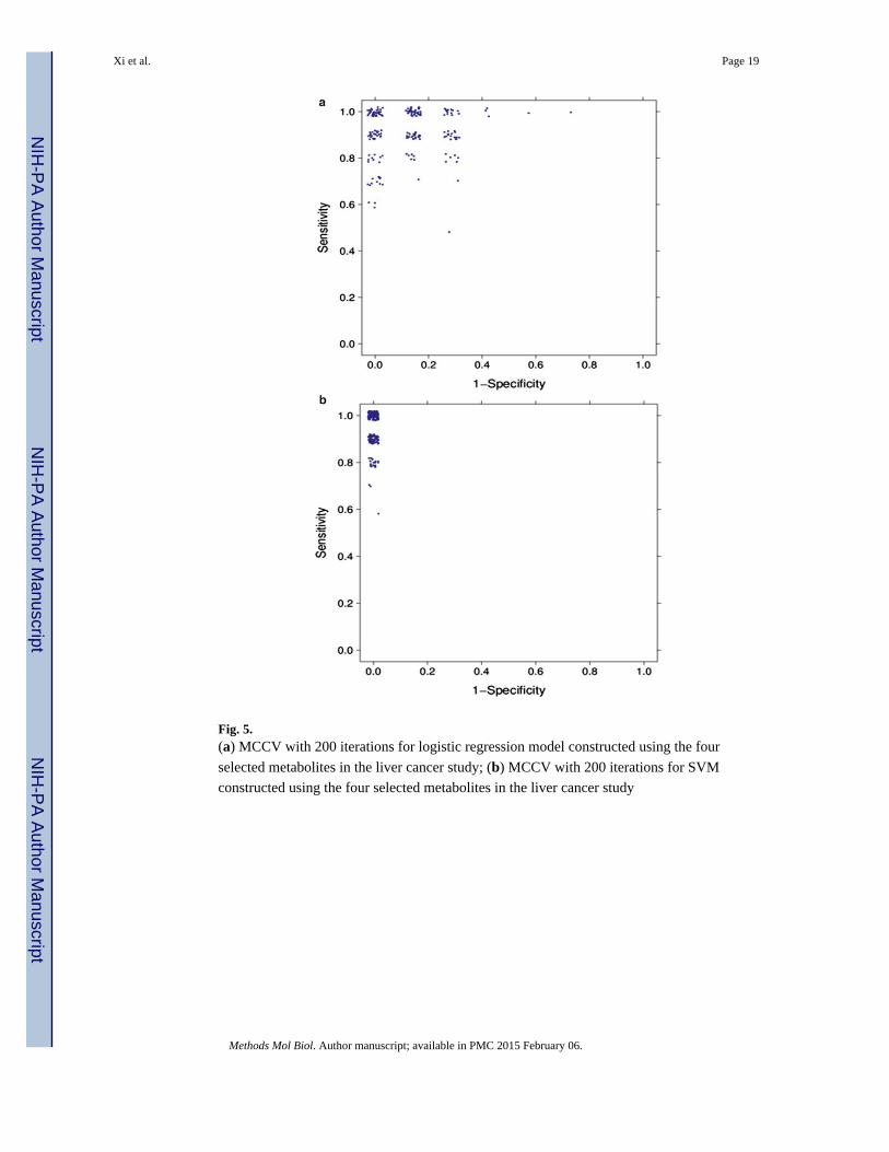
Fig. 5. (a) MCCV with 200 iterations for logistic regression model constructed using the four

selected metabolites in the liver cancer study; (b) MCCV with 200 iterations for SVM

constructed using the four selected metabolites in the liver cancer study

Xi et al.


NIH

-PA

Author M

anuscriptN

IH-P

A A

uthor Manuscript

NIH

-PA

Author M

anuscript

NIH

-PA

Author M

anuscriptN

IH-P

A A

uthor Manuscript

NIH

-PA

Author M

anuscript

Xi et al.

Table 1

List of metabolites with significant mean changes between HCC and HCV patients

Metabolite a FC p-Value

Tyrosine 0.8 0.016

Phenylalanine 0.9 0.013

Glycerol 0.8 0.018

Methionine 0.7 0.0032

Creatine 2.1 0.029

Homocysteine 0.8 0.036

2-Deoxyguanosine 0.3 0.015

Xanthine 0.8 0.011

1-Methyladenosine 1.4 0.011

N2,N2-Dimethylguanosine 0.5 0.0018

5-Hydroxymethyl-2′-deoxyuridine 1.5 0.00088

1-Methylinosine 0.5 0.0075

1-Methylguanosine 0.6 0.0078

N-Carbamoyl β-alanine 0.7 0.016

Aconitic acid 0.7 0.029

Uric acid 0.7 0.0069

aFC: mean fold change (HCC/HCV)


nih public access abstract metabolomics data methods …xbw/research/nihms656480.pdf · statistical...

Documents