nhts weighting report
TRANSCRIPT

2017 NHTS Weighting Report
Task P
Authors
Shelley Brock Roth
Jill DeMatteis
Yiting Dai
December 1, 2017
Prepared for:
Federal Highway Administration
Washington, DC
Prepared by:
Westat
An Employee-Owned Research Corporation®
1600 Research Boulevard
Rockville, Maryland 20850-3129
(301) 251-1500
2017 NHTS Weighting Report i
Table of Contents
Section Page
1 Overview ..................................................................................................................................... 1-1 2 Household Level Weights—Base Weights ............................................................................. 2-1
2.1 Full Sample Base Weights ........................................................................................... 2-1 2.2 Replicate Base Weights ................................................................................................ 2-2
3 Household Level Nonresponse Adjustments ........................................................................ 3-1
3.1 Recruitment Adjustment for Unknown Eligibility and Nonresponse Adjustments within Geographic Adjustment Cells ......................................................................... 3-4
3.2 Retrieval Nonresponse Adjustments within Geographic Adjustment Cells ........ 3-5 3.3 Specification of Nonresponse Adjustment Cells ..................................................... 3-6
4 Raking Procedures—Household Level ................................................................................... 4-1
4.1 Raking Dimensions for Households .......................................................................... 4-3 4.2 Construction of Control Totals for Time Dimensions ........................................... 4-4
5 Person-Level Raking Adjustments ........................................................................................... 5-1 6 Other Weights and Quality Control of the Weights ............................................................. 6-1
6.1 Vehicle and Trip Weights ............................................................................................ 6-1 6.2 Quality Control of the Weighting Process ................................................................ 6-1
References ......................................................................................................................................... 7-1 A Characteristics to be Used to Form Recruitment Nonresponse Adjustment Cells ......... A-1 B ABS Frame and Recruitment Questionnaire Characteristics to be Used to Form
Household Retrieval Nonresponse Adjustment Cells .......................................... B-1 C Construction of Control Totals from the American Community Survey ......................... C-1 D Imputation Plan ........................................................................................................................ D-1 E Summarization of Household Raking Steps (7-Day Weights)............................................ E-1 F Summarization of Person-Level Raking Steps .......................................................................... 1

2017 NHTS Weighting Report 1-1
The sample design for the 2017 National Household Travel Survey (NHTS) is described in the
December 31, 2015 document ‘Task C: Sample Design’ (Task C Deliverable,
Task_C_Sample_Design FINAL 20151231.docx). The weighting report for the 2017 NHTS
decribes the construction of the weights and provides some results. The methodology used was
based roughly on the weighting procedures that were executed for the 2009 NHTS. This approach is
appropriate for the NHTS 2017 because weighting procedures such as the ones used for the 2009
NHTS retain their robustness regardless of survey mode. These are standard procedures that apply
to data collected in household surveys, and include basic steps of calculating the inverse of the
selection probability for each sampled address as a base weight, adjusting the base weights for
eligibility and nonresponse, and poststratifying the adjusted weights to reliable external source data,
such as Census data. Some of the specifics of the adjustments, such as the adjustment for unknown
eligibility, depend on the mode, and in such situations, the adjustments have been modified as
appropriate. Otherwise, the weighting methodology was kept as similar as possible to 2009 also to
allow an easier examination of travel trends.A few of the changes between 2009 and 2017 and key
aspects of 2017 procedures are noted below:
The 2017 study required that every household member age 5 and older complete a
retrieval interview in order for the household to be considered complete.
One set of weights was produced that can be used with the combined national sample and Add-on study samples, or separately for each Add-on’s geographic area. Both 7-day and 5-day weights were provided for the Add-on areas.
In 2009, independent selections were used to select the Add-on and national samples. In 2017, there was no need for independent selections (since all sample design decisions for both the National portion and the Add-on samples were finalized prior to selection of the addresses), so it was not necessary (or appropriate) to use composite estimation, as was done in 2017.
The nonresponse analysis work to conducted under Task P included a concurrent nonresponse bias analysis that was completed before weighting was finalized, to allow for results from that work to inform the weighting process.
The NHTS 2017 survey design is quite complex in that there are numerous pieces which make up
the full NHTS 2017 sample, including a national portion, 13 Add-on area portions, and two time
Overview 1
2017 NHTS Weighting Report 1-2
Overview 1
periods when addresses were selected from the address-based sampling vendor (referred to as
“Sample Groups 1 and 2”). With regard to the two time periods, Sample Groups 1 and 2 were
structured such that the Sample Group 1 was selected before data collection commenced and
Sample Group 2 was selected about halfway through data collection efforts, to account for response
rates up to that point. The timing of Sample Groups 1 and 2 allowed for operational flexibility in
trying to maximize response and achieve desired sample yield targets. The sampling documentation
(Task C deliverable, see above) describes this process.
Similar to NHTS 2001 and NHTS 2009, we performed a household-level nonresponse adjustment,
which consisted of adjusting the weights for characteristics that were determined to be related to
response propensity. We also did household-level raking to independent household control totals,
such that the final raked weights sum to known benchmark controls from the American Community
Survey (ACS), both 2015 1-year and 2011-2015 5-year data. Using both approaches allowed us to
use a different cell structure such as using Census tract-level characteristics (which are available for
both respondents and nonrespondents) to adjust for recruitment nonresponse, and variables such as
Hispanic origin and number of vehicles (which are available only for respondents) to adjust for
population undercoverage.
Also as in NHTS 2001 and NHTS 2009, we estimated variances (as a way of giving data users and
readers an indication of the precision of the survey estimates) using a jackknife replication
methodology. Replication, specifically the jackknife method, is described in Section 2.2.
Household weights, person-level weights,travel-day trip-level weights and vehicle weights were
produced. The household-level weights are designed to represent all households in the study area,
and were produced for the National sample (7-day only) and for all Add-on areas (7-day and 5-day).
The person-level weights are designed to represent all persons in the study area. These also were
produced for the National sample (7-day only) and for all Add-on areas (7-day and 5-day). As was
the case in the 2001 NHTS and the 2009 NHTS, all of the weights produced are “annual” weights.
The overall steps in the weighting process were as follows (see Exhibit 1 below):
Construction of base weights—the base weights are the reciprocals of the probabilities
of selection within each sampling stratum (for the national sample) or substratum (for Add-ons) (see Task C: Sample design for stratum definitions);

2017 NHTS Weighting Report 1-3
Overview 1
Construction of jackknife replicate weights—the replicate weights are designed to allow the user to easily produce valid jackknife variance estimates based on the sample design, using software designed for the analysis of complex sample survey data;1
Household-level nonresponse adjustments (separate adjustments for unit nonresponse to the recruitment and retrieval efforts, done within each Add-on area and the rest of the Census division separately (see table 1 in section 3 for geographic definitions);
Household-level raking and trimming (using the household-level nonresponse adjusted weights);
Person-level raking and trimming;
Computation of vehicle and trip weights; and
Inclusion of the final weight variables in the preparation of data files for analysis--a set of files will be delivered to the specifications of FHWA, including all relevant final weights and identifiers.
The listing of chapters roughly follows the order that the weighting process was carried out. Chapter
2 describes the process for computing household-level base weights within each sampling stratum,
which were defined during the sample design process and used for selection of addresses. Chapter 3
describes adjustments for nonresponse at the household level, done within the separate studies and
sample groups. Chapter 4 describes the raking procedure at the household level. Chapter 5 describes
the person-level raking adjustments. Finally, Chapter 6 describes special weights for vehicles and
trips.
1 Replicates simulate multiple samples from our single NHTS sample, allowing for estimation of variances. There are several methods, but the jackknife method works well for our data due to its sample design. Software such as WesVar, or the survey procedures in SAS, will easily compute appropriate standard errors using the replicate weights.

2017 NHTS Weighting Report 1-4
Overview 1
Exhibit 1 Flowchart of NHTS Weighting Procedures
NHTS weighting flowchart
Households
HH retrieval 5-day respondents
HH ret rieval 7-day respondents
5-day vehicle weights
7-dayvehicle weights
Persons
Person raked and trimmed weights
Person raked and trimmed weights
Trip weights Trip weights
National and Add-onsAdd-ons
HH 7-day raked and trimmed weights
HH ret rieval 7-day respondents
A
HH base full-sample/replicateweights
all sampled addresses
all sampled addresses
HH unknown eligibility adjustment weights
all eligible addresses
HH recruitment nonresponse
adjustment weights
HH recruitment respondents
HH retrieval nonresponse
adjustment weights
HH retrieval respondents
A
Al l persons age 5+ in the HH that
completed retrieval
Al l persons age 5+ in the HH that
completed retrieval
HH retrieval 5-day respondents
HH 5-day raked and trimmed weights
2017 NHTS Weighting Report 2-1
The primary component of the base weight is the inverse of the probability of selection of the
address in the given sampling stratum from the sampling frame.
The sample design for each stratum (or substratum) (see Task C: Sample Design for stratum and
substratum definitions) is an equal probability sample of addresses, that is, all addresses had an equal
chance of selection, from the Address-Based Sample (ABS) sampling frame for the
stratum/substratum (the strata/substrata are defined in the December 31, 2015 sample design plan,
see Task C: Sample Design). Although the sample was selected via two independent selections as
described earlier (to ensure the sample yield, that is, the number of completed surveys, would be as
close as possible to the target number of completed surveys, the differences between the two
sampling frames were very minimal. Westat took into account the response rates (our experience
from the first part of the sample) when deciding on sample sizes for the second part of the sample,
to make sure we would hit our estimated targets. Additionally, different proportions of the sample
were released from the two selections. All of the differences (between the two selections and their
associated releases) are simply operational in nature, so in order to smooth the sampling rates, for
weighting purposes, the sample was treated effectively as a single selection from a single frame2. The
second sample selection was deduplicated against the first sample, so that no address could be
sampled twice.
2.1 Full Sample Base Weights
The base weight is the inverse of the selection probability for the address. Note that the sum of the
base weights for a given sampling stratum provides an estimate of the total number of addresses in
the sampling stratum from which the addresses were drawn. The sum of the base weights across all
sampling strata provides an estimate of the total number of addresses in the frame.
2 The two parts of the sample were drawn from a single frame, the USPS file of addresses that is maintained by the sampling vendor Westat uses. This frame is updated on a monthly basis. In Westat’s experience, the monthly updates are quite small. Accounting for the separate selections would have introduced considerable variation in the weights (due to variations in the separate probabilities of selection) that is not necessary considering that they yielded, effectively, a single sample (released on a weekly basis). Given that, we treated the two independent samples as if they had been selected in a single draw from a single frame.
Household Level Weights—Base Weights 2
2017 NHTS Weighting Report 2-2
Household Level Weights—Base Weights 2
2.2 Replicate Base Weights
Replicate base weights were also computed for each household in each sampling stratum separately.
Replicate base weights are important because they simulate multiple samples from our single NHTS
sample, allowing for estimation of variances of survey estimates.
Variance strata are geographic areas that were used in the weighting process to make sure the
weights were created in a manner that is related to the sample design, and were formed using
National sample only states and the thirteen Add-on areas separately.
Replicate base weights were computed using similar methodology to what was used for the 2009 and
the 2001 NHTS weights. We used the stratified jackknife replication method (JKn; see WesVar® 4.2
User’s Guide (2002)) to create G=98 replicates3. We numbered each sampled address from 1 to 7
within each of the fourteen sample areas, the thirteen areas determined by the Add-ons and the rest
of the nation, in selection order within the sample areas (variance strata) to form variance units. We
ensured that there was at least one completed interview within each variance stratum. Replicates
were formed within each variance stratum by deleting one variance unit at a time and multiplying the
weights for the other variance units in the same variance stratum as the deleted unit by
𝑛ℎ (𝑛ℎ − 1)⁄ , where 𝑛ℎ is the number of variance units in the variance stratum with the deleted unit
(in this case, 𝑛ℎ = 7). In other words, within each of the 14 variance strata, all replicate weights are
equal to the full-sample weight except for those in the variance stratum containing the deleted
variance unit for the replicate, which are ‘perturbed’ by setting the deleted variance unit’s weight to
zero (for that replicate) and multiplying the weights of the other variance units in that variance
stratum by 𝑛ℎ (𝑛ℎ − 1)⁄ . These procedures resulted in 7 replicates created in each of the 14 sample
areas (variance strata), for a total of 98 replicates.
Full sample and replicate base weights were used as the starting weights for the household level
nonresponse adjustments. The full-sample weights and each of the replicate weights received the
same set of adjustment steps, as described in the remaining sections of this report.
3 The goal of replication is to create a sufficient number of “simulated” samples such that precision can be gained in variances of the survey estimates. Within each of the fourteen sample areas, 7 variance units were assigned, which yielded a total of 14*7=98 replicates. For a survey of this size, 98 replicates is sufficient.

2017 NHTS Weighting Report 3-1
Nonresponse to surveys unfortunately is a major and continuously growing problem with virtually
every survey. Our approach to controlling unit nonresponse has two parts: a nonresponse bias
analysis where we analyzed survey nonresponse and the potential for bias, and the development of
appropriate nonresponse adjustments to the weights based on the results of this analysis.
The nonresponse adjustments are based on a paradigm generally used in survey research (Oh and
Scheuren 1983). Under this paradigm, nonresponse is treated as a subsampling process within
carefully selected nonresponse-adjustment cells. The nonresponse-adjustment cells are selected to be
heterogeneous in response propensity (the probability of responding) across cells, and homogeneous
in response propensity within cells. The nonresponse bias analysis informed this cell selection
process by finding characteristics which were related to response propensity (propensity to
cooperate at the recruitment level, propensity to cooperate at the retrieval level). The final
nonresponse adjustments are equal to the inverse of the base-weighted response rates within the
selected nonresponse adjustment cells. These nonresponse adjustment cells are nested within the
strata used in sample selection. The cells were not smaller than 29 sample units, as cells with limited
numbers of sample units generate unreliable (highly variable) nonresponse adjustments. In addition,
cells with very low weighted response rates or very small size were collapsed with other cells to
avoid extreme weighting adjustments, which can introduce too much variability4.
Nonresponse adjustment was done separately at the recruitment level (recruitment nonresponse)
and the retrieval level (retrieval nonresponse within recruited households).5 The cell structure
differed between the stages since response patterns were quite different for the different stages of
data collection. Additionally, the nonresponse adjustments for recruitment nonresponse included an
4 There is not a pre-defined cut-off but we did not want to create weights that were too extreme. Cells with particularly low response rates would get higher adjustments factors which can result in large weights. We carefully reviewed the adjustment factors for all cells and determined where collapsing was needed. 5It is standard practice to adjust for nonresponse at each phase in a multi-phase study. For each phase of data collection, we weight up the respondents so that they represent the population, and this weighting up is done under the pseudo-randomization paradigm (which treats nonresponse as another phase of sampling, as described in the Oh & Scheuren reference). For NHTS it is particularly crucial to adjust for nonresponse at the recruitment level, because that is where the majority of our nonresponse (and potential bias) is occurring.
Household Level Nonresponse Adjustments 3

2017 NHTS Weighting Report 3-2
Household Level Nonresponse Adjustments 3
adjustment reflecting the proportion of cases with unknown eligibility that are estimated to be
eligible.
The variables used for these unit nonresponse adjustment steps must be available for both
respondents and nonrespondents. Thus, the data available to adjust for recruitment nonresponse
were mainly aggregate variables appended to the address based on its geocoded location, e.g., Census
tract-level variables (see Appendix B for a list of variables that were considered for this adjustment).
A few items from the ABS frame were also included for consideration. While the ABS vendor can
also append household- and person-level characteristics, research has shown that these appended
variables are incomplete and often inaccurate (Roth, Han, and Montaquila 2013). Based on the
nonresponse bias analysis, we determined characteristics to use to define adjustment cells6 (those
characteristics which are related to recruitment response propensity and are also related to key travel
variables from the NHTS, such as household vehicle trips, person trips, average number of daily
trips per household, average annual vehicle miles of travel per household, or average time spent
driving on any trip).
For the retrieval nonresponse-adjustment cells, we also included information from the recruitment
questionnaire, such as household size, race and ethnicity of reference person, home ownership,
location, home type, and number of vehicles in household. The 2009 NHTS nonresponse bias
report showed that many recruitment variables are associated with retrieval response; we re-
examined this as part of the nonresponse bias analysis for the 2017 NHTS. We found that many of
these variables were appropriate to be used in nonresponse cell generation.7
Geographic adjustment cells were defined geographically as state, for states where the Add-on area
encompasses the entire state (specifically, AZ, CA, GA, MD, NC, NY, SC, and WI); Add-on area,
for the sub-state-level Add-ons (Des Moines, Iowa Northland, Indian Nations (OK), and North
Central (TX); Texas, which includes the TX DOT Add-on as well as the remainder of the state, or
6 Tract-level variables and ABS frame variables were assessed during the nonresponse bias analysis to see if they were a good fit for our nonresponse adjustment process. Data that are available for all sampled addresses to adjust for recruitment nonresponse has to be used for this adjustment. The nonresponse bias analysis in conjunction with Westat’s extensive experience in adjusting for nonresponse to surveys results in adjustments to the weights that will ultimately provide for better (less biased, more accurate) estimates and variances. 7 The objective was to find variables that are associated with both key survey outcome variables and response propensity. To examine association with response propensities, we used a SAS procedure, HPSPLIT, which uses chi-square testing at each split to identify characteristics that are (conditional on previous splits) significantly associated with response propensity.
2017 NHTS Weighting Report 3-3
Household Level Nonresponse Adjustments 3
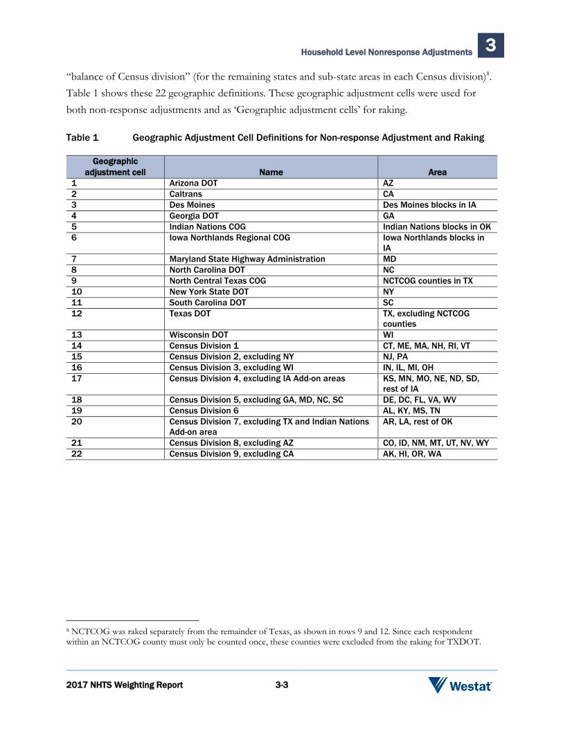
“balance of Census division” (for the remaining states and sub-state areas in each Census division)8.
Table 1 shows these 22 geographic definitions. These geographic adjustment cells were used for
both non-response adjustments and as ‘Geographic adjustment cells’ for raking.
Table 1 Geographic Adjustment Cell Definitions for Non-response Adjustment and Raking
Geographic
adjustment cell Name Area
1 Arizona DOT AZ
2 Caltrans CA
3 Des Moines Des Moines blocks in IA
4 Georgia DOT GA
5 Indian Nations COG Indian Nations blocks in OK
6 Iowa Northlands Regional COG Iowa Northlands blocks in
IA
7 Maryland State Highway Administration MD
8 North Carolina DOT NC
9 North Central Texas COG NCTCOG counties in TX
10 New York State DOT NY
11 South Carolina DOT SC
12 Texas DOT TX, excluding NCTCOG
counties
13 Wisconsin DOT WI
14 Census Division 1 CT, ME, MA, NH, RI, VT
15 Census Division 2, excluding NY NJ, PA
16 Census Division 3, excluding WI IN, IL, MI, OH
17 Census Division 4, excluding IA Add-on areas KS, MN, MO, NE, ND, SD,
rest of IA
18 Census Division 5, excluding GA, MD, NC, SC DE, DC, FL, VA, WV
19 Census Division 6 AL, KY, MS, TN
20 Census Division 7, excluding TX and Indian Nations
Add-on area
AR, LA, rest of OK
21 Census Division 8, excluding AZ CO, ID, NM, MT, UT, NV, WY
22 Census Division 9, excluding CA AK, HI, OR, WA
8 NCTCOG was raked separately from the remainder of Texas, as shown in rows 9 and 12. Since each respondent within an NCTCOG county must only be counted once, these counties were excluded from the raking for TXDOT.
2017 NHTS Weighting Report 3-4
Household Level Nonresponse Adjustments 3
3.1 Recruitment Adjustment for Unknown Eligibility and
Nonresponse Adjustments within Geographic Adjustment
Cells9
Recruitment nonresponse occurs when an eligible10 sampled address does not complete the
recruitment instrument. A completed recruitment instrument is one for which the respondent has
completed the household and vehicle enumeration parts of the instrument.
In general, nonresponse adjustments are equal to the summation of base weights11 for all eligible
addresses divided by the summation of base weights for all recruitment respondent households,
within the cells we define as a result of nonresponse bias analysis. The numerator includes all sample
units which are definitely identified as being eligible (respondent or not), and exclude all sample
units which are definitely identified as being ineligible.
Because the survey weights should account for only the eligible population, it is important to
identify ineligibles and exclude them from the weighting process. When mail is returned to us from
an address, we are able to determine the eligibility of the address. If a household completes the
recruitment instrument and returns it, or the household writes something on the instrument
indicating they do not wish to participate and returns it, we know the mailing has reached an eligible
address. If the recruitment mailing is returned by the USPS with a message indicating an
undeliverable address, we know the mailing has reached an ineligible address.
Across all categories of addresses12, there is one general category of addresses, unreturned mail,
where eligibility is uncertain at the completion of the recruitment process. Since we do not know if
unreturned mail addresses are eligible or not, the number of eligible addresses among them is
estimated. This estimate is then used in the recruitment nonresponse adjustment process to adjust
the weights accordingly. For the set of addresses for which eligibility is unknown, the estimated
9 The study design resulted in a large amount of unreturned mail for which Westat is unable to determine that address’s eligibility. Through the process described here, we estimate the proportion of those that are eligible, and also ineligible. This is important because the goal is for the weighted sample to represent eligible households (and persons within those households) but not represent ineligible addresses.
10 Ineligibility in this study arises from vacant addresses, vacation homes, invalid addresses, or addresses that are not dwelling units.
11 Sections 2.1 and 2.2 result in full sample and replicate base weights. Those are the weights we adjusted for unknown eligibility.
12 Categories include Residential, Business, Vacant, Seasonal, Educational (e.g., college dorm), Throwback (city style address that does not accept mail delivery), Drop point (single delivery point servicing multiple residences), and unreturned mail.

2017 NHTS Weighting Report 3-5
Household Level Nonresponse Adjustments 3
portion of eligible addresses e described below was computed, and added to the numerator described
in the previous paragraph. This is similar to the approach that was used to treat telephone numbers
in the older RDD sampling approach where the phone number rang but was never answered.
The approach to estimating eligibility can be referred to as the “backing out” approach to estimating
e. Here we use the estimate of the total number of households within each geographic adjustment
cell (TACS), the total number of respondents in each geographic adjustment cell (TR), the total
number of nonrespondents in each geographic adjustment cell (TNR), and the total number of
unknown eligibility cases in each geographic adjustment cell (TU) to estimate e as follows:
�̂�𝐴𝐶𝑆 = �̂�𝑅 + �̂�𝑁𝑅 + 𝑒�̂�𝑈 ,
where �̂�𝐴𝐶𝑆 is estimated number of households from most recent (2015) ACS. So
𝑒 = (1
�̂�𝑈) (�̂�𝐴𝐶𝑆 − �̂�𝑅 − �̂�𝑁𝑅).
The recruitment nonresponse adjustment cells are intended to be homogeneous in recruitment
response and contact propensity within the cells and heterogeneous in recruitment response and
contact propensity across cells. The cells were generated after a selection of cells using the SAS
procedure HPSPLIT (a binary search algorithm software routine), as discussed in Section 3.3 below.
The recruitment nonresponse adjusted weight for each recruitment respondent is equal to the base
weight multiplied by the recruitment nonresponse adjustment for the nonresponse cell containing
the respondent.
3.2 Retrieval Nonresponse Adjustments within Geographic
Adjustment Cells
A household is considered complete if the retrieval survey has been completed for all household members ages 5
and older. Otherwise, the household is viewed as a nonrespondent at this level. Therefore, in all
following discussions, “retrieval response” refers to having completed retrieval surveys for all
household members ages 5 and older.

2017 NHTS Weighting Report 3-6
Household Level Nonresponse Adjustments 3
To adjust for retrieval nonresponse, each completed household receives an adjustment for
nonresponding households that completed the recruitment survey but not the retrieval survey; this
adjustment is equal to the reciprocal of the weighted retrieval response rate in its adjustment cell.
These adjustment cells were selected to be as heterogeneous in terms of retrieval response rates
across cells as possible, and as homogeneous in terms of retrieval response rates within cells as
possible. The cells were selected following an analysis of household characteristics found to be
correlated with completion rates (see Section 3.3 below).
As compared to recruitment nonrespondents, there is more information available about retrieval
nonrespondents (households that have not completed the retrieval survey). This extra information,
such as home ownership, vehicle count, and age, gender, race/ethnicity, and educational attainment
for the recruitment respondent, comes from the completed recruitment instrument.
The nonresponse adjustments for each cell is the weighted sum of recruitment responding
households within the cell divided by the weighted sum of completed households within the cell.
The weights used in computing these weighted sums were the recruitment nonresponse adjusted
weights described in the previous section 3.1. The final household-level nonresponse adjusted
weight for each completed household is the recruitment-nonresponse-adjusted weight multiplied by
the retrieval nonresponse adjustment for the retrieval nonresponse cell containing the household.
3.3 Specification of Nonresponse Adjustment Cells
The SAS procedure HPSPLIT was used to define nonresponse cells within each sampling stratum
for both recruitment nonresponse and retrieval nonresponse separately. HPSPLIT is a high
performance SAS procedure that builds classification trees to model response. More details on the
procedure can be found at
https://support.sas.com/documentation/onlinedoc/stat/141/hpsplit.pdf.
For recruitment nonresponse adjustment cells, the HPSPLIT procedure created a classification tree
within each geographic adjustment cell separately. The algorithm avoided constructing cells with a
sample size smaller than 30, and avoided adjustments significantly larger than five times the mean
adjustment for the stratum. In cases of violation of these norms, the cells were collapsed such that
the minimum cell size of 30 requirement was met, and such that the adjustment factors were not
larger than five times the mean adjustment.

2017 NHTS Weighting Report 3-7
Household Level Nonresponse Adjustments 3
Potential cells were generated based on ABS frame information and variables that could be linked to
the sample (e.g., Census tract-level variables). The nonresponse cells were dichotomous cells (above-
median and below-median) using weighted medians of ABS frame characteristics within stratum.
For example, one set of cells was households with an appended telephone number for a particular
stratum. Not every set of cells was chosen: only those that registered as significantly correlated to
response propensity within the stratum, and which satisfied the criteria defined in the previous
paragraph. Also, not every frame characteristic was tested: only those that registered as important in
the nonresponse bias analysis were included in the analysis. The listings of characteristics included in
the recruitment nonresponse bias analysis (which was subsequently tested for cell formation by
HPSPLIT) is given in Appendix B.13
For retrieval nonresponse adjustment cells, HPSPLIT searched using the characteristics given in the
tables in Appendix B. Most of these are recruitment questionnaire variables, but some are ABS
frame characteristics.
The final nonresponse adjusted household-level weights were used as the input weights for the
household-level raking procedures outlined in section 4.
13 The list is based on the Census tract-level characteristics used in the 2009 NHTS weighting process, updated for 2017 to add two variables from the ABS frame that were useful for nonresponse bias analysis, which arewhether a phone number could be matched to the address and type of dwelling unit: single- or multi-family.

2017 NHTS Weighting Report 4-1
ABS frames provide excellent coverage of the population as a whole; for surveys like the NHTS that
make contact with households via mail (so that households with nonlocatable addresses such as PO
box addresses or rural route addresses are included), the coverage is estimated to be about 98
percent (see Link et. al., 2010). However, coverage varies among different types of areas (e.g., as
described by the four primary sampling strata ). It is possible to adjust for differential coverage
through a calibration weighting process called “raking,” where the weights are iteratively adjusted to
independent controls totals for various demographic categories14. The process has the effect of
differentially adjusting the weights of the sampled households within groups of demographically
similar households, so that the total sum of weights for the sampled households equals the
corresponding independent control totals for all households (including those not covered by the
ABS sample).
Raking and trimming steps were performed iteratively at the household level15. The starting point
was the household retrieval nonresponse adjusted weights described in Section 3. The trimming
steps included a ‘pre-trim’ step preceding the first household raking step, and a ‘post-trim’ step
following each household raking step. Each trimming step was applied within the geographic
adjustment cells.
The pre-trim step for each geographic adjustment cell consisted of checking for weights that were
more than 3.0 times the median weight.16 If less than 1% of the weights fell into this category, then
all such weights were trimmed back to equal the cutoff (3.0 times the median weight for the
stratum). If more than 1% of the weights fell into this category17, then the largest 1% set of the
weights were trimmed back to equal the 99th percentile of the weights.
14 Control totals were comprised of 2015 ACS 1-year data where possible and 2011-2015 5-year data adjusted to 1-year totals where geographies were too small to use the 1-year data directly. In a few special cases we used the 2010 Census SF1, also adjusted to 1-year ACS totals. Please see section 4.1 for details on the control totals sources.
15 The idea of trimming is to limit the size of the weight that can be associated with a single household so that it does not have too much influence on the estimates.
16 This is the median value of all of the household level raked weights after the raking adjustment. If any household raked weight violated 3*median threshold prior to trimming, it was trimmed as described.
17 The number of weights affected by this rule was 1% of the number of sample units, rounded up to the smallest larger integer. For example, if the sample size was 120, then the number of trimmed weights was 2 (1.2 rounded up). In
Raking Procedures—Household Level 4
2017 NHTS Weighting Report 4-2
Raking Procedures—Household Level 4
The post-trim steps follow the raking steps and were also done within each geographic adjustment
cell, and targeted for trimming any weights that were 4.5 times smaller or 4.5 times larger than the
median weight for the geographic adjustment cell. A maximum of 2.5% of the weights were
trimmed on the high side and a maximum of 2.5% of the weights were trimmed on the low side for
each post-trim step18. If more than 2.5% of the weights were greater than 4.5 times the median
weight (less than 4.5 times the median weight), then the largest (smallest) 2.5% of the weights were
trimmed back to the 97.5th percentile (the 2.5th percentile). This procedure with its associated limits
was adopted for the 2009 NHTS after extensive expert review, and therefore was followed for the
2017 NHTS19.For more information on trimming procedures, see Potter (1993).
The iteration of raking and trimming steps was complete when all of the trimming factors for that
final putative trimming step were between 0.99 and 1.01. In other words, once raking converged and
all trimming factors were between 0.99 and 1.01, the weights were considered final. A flag indicating
that a weight was trimmed is provided on the delivery files.
This raking and trimming process has a number of “dimensions.” The dimensions are discussed in
detail in section 4.1 below. The weights were adjusted to equal the totals within the cells for each
dimension in an iterative process, until the process converged, and every dimension’s cell totals
equal (to within the specified tolerance) the independent control totals. Each household raking step
in the cycle was done to a tolerance of ±1, i.e., the weighted household totals were raked until they
were within 1 of the household control totals. If convergence was not achieved initially, cells were
collapsed (within dimensions) until convergence was reached.
particular, there was always be at least one weight trimmed if any weight exceeds 3.0 times the median weight. The actual percentage of trimmed weights then could be slightly larger than 1%.
18 This count of trimmed weights was 2.5% of the number of sample units, rounded up to the smallest larger integer. For example, if the sample size was 100, then the maximum high side or low side number of trimmed weights was 3 (2.5 rounded up). The actual percentage of trimmed weights on the high and low side could be slightly larger than 2.5%.
19 The procedures and thresholds are set with the goal of reducing the impact in terms of the effect on variances and influence of particular observations on estimates. Limiting the amount of trimming performed is also a goal since trimming introduces bias.

2017 NHTS Weighting Report 4-3
Raking Procedures—Household Level 4
4.1 Raking Dimensions for Households
We used the 2015 American Community Survey (ACS) data to develop the control totals. First,
overall totals were obtained at the Census division level20. Within Census division, counts were
derived from one-year 2015 ACS estimates where possible, using 2011-2015 five year estimates
where necessary to obtain distributions for areas for which 2015 one-year ACS estimates were not
available, within geographic adjustment cell, or geographic adjustment cell, definitions as described
in table 1 above (section 3). In a few instances, the 2010 Census SF1 data were necessary to obtain
distributions for areas defined by Census blocks, such as the Iowa Northlands Add-on area.
For the larger counties, the ACS provides population estimates based on one year of data alone (the
most recent year). For many other counties, the ACS only provides estimates as moving averages
based on the five most recent years. The five-year estimates (or Census SF1 counts) were only used
to ‘fill in’ whatever distributions were not available from the one-year data (only percentages were
used). Then, for each raking dimension, percentages within geographic adjustment cell totals were
applied to the Census division totals to obtain geographic adjustment cell-level totals that summed
to the Census division total. Appendix C describes in further detail the process of computing control
totals.
The raking dimensions were as follows21.
(1) Geographic adjustment cell *MSA/heavy rail sampling stratum
(2) Geographic adjustment cell * race (Black; non-Black for recruitment respondent)
(3) Geographic adjustment cell * Hispanic origin (Hispanic; non-Hispanic for recruitment respondent)
(4) Geographic adjustment cell * Owner/Renter (Owner; Renters and others)
(5) Geographic adjustment cell * Number of Vehicles (0, 1, and 2 or more Vehicles)
(6) Geographic adjustment cell * Month
(7) Geographic adjustment cell * Day of Week
20 Although Census Divsions are larger than the state level geography, this level of geography was selected to ensure that we were able to get convergence during raking.
21 These dimensions were ordered by importance. A higher number in the ordering indicates the dimension was collapsed sooner if there were convergence problems.

2017 NHTS Weighting Report 4-4
Raking Procedures—Household Level 4
(8) Geographic adjustment cell * Household size * Number of workers in the household (1-person household with 0 worker, 1-person household with 1 worker, 2-person household with 0 workers, 2-person household with >=1 workers, 3-preson household with 0 workers, 3-person household with >=1 workers, 4-person and more household with 0 workers, and 4-person and more household with >=1 workers)
When convergence failed, the design called for the collapsing of cells (e.g., day to
weekday/weekend), then variables within dimensions, and finally the elimination of a dimension.
The raking dimensions for households focused on geography and overall household characteristics.
When person-level characteristics were used, such as race and ethnicity, recruitment respondent
information was used. In general, levels were collapsed if there were fewer than 8 retrieval
households for the level.
4.2 Construction of Control Totals for Time Dimensions
At this point in the processing, adjustments for month and day were applied to the raked household
weights resulting from section 4.122. Those household weights were adjusted to account for the 12
months of data collection. Then those weights were adjusted to create both 7-day and 5-day sets of
final household raked weights, as outlined next.
The time dimension control totals sum to the geographic adjustment cell household total for each
geographic adjustment cell23. Each month was allocated approximately 1/12 of the household total,
so that each month has an equal weight in the final estimator (the sum of household weights with
travel dates corresponding to one month will be made equal to about 1/12 of the household total
for each geographic adjustment cell). For 7-day weights, each day of the week was allocated 1/7 of
the household total. For 5-day weights, each weekday (Monday through Friday) was allocated 1/5 of
the household total (and only responding households with weekday travel days were included in the
raking adjustment). However, the 5-day weights were also adjusted to exclude the following holidays,
as specified by the Federal Highway Administration:
22 The NHTS is designed to collect data evenly over a 12-month period, but even with diligent management, this was not exact. This adjustment was done to ensure that each month of the year represented approximately 1/12 of the responding households. Similar adjustments were done to ensure that data were represented equally across all 7 days of the week for the 7-day weights, or all 5 days of the week for 5-day weights.
23 The final weighted household total within each geography from table 1 were maintained even after adjustments for time dimensions.

2017 NHTS Weighting Report 4-5
Raking Procedures—Household Level 4
Monday May 30, 2016 – Memorial Day
Monday July 4, 2016 – Independence Day
Monday, Sept 5, 2016 – Labor Day
Thursday, Nov 24, 2016 – Thanksgiving Day
Monday, December 26, 2016 – Christmas Day
Monday, January 2, 2017 – New Year’s Day
Monday, January 16, 2017 – Martin Luther King Birthday
All analyses using the 5-day weights will need to exclude data for travel days falling on these dates;
that is, the 5-day (weekday) weights represent travel on all weekdays in the year excluding these holidays.
Analysts (using either the 5-day or 7-day weights) may also choose to exclude other days from their
analyses. However, they may not add the excluded holidays listed above back into analyses using the
5-day weights, as these dates do not have 5-day weights.
These adjustments result in 5-day and 7-day sets of final raked household-level weights. Both of
these sets of weights were used as inputs to the person-level raking and were carried through the
remaining procedures.

2017 NHTS Weighting Report 5-1
The aim of the survey was to complete retrieval interviews for each person age 5+ within each of
the recruited households. In terms of sampling, this meant that every person age 5+ in the
household had a probability of selection equal to that of the household. In principle, then, each
person’s base weight was equal to the household base weight. Since the people within a household
were all selected along with the household, the starting weight for person adjustments was the final
adjusted household weight from section 4. Both 5-day and 7-day household-level raked weights
from section 4 were processed (separately) to create person-level raking adjustments, resulting in the
final person-level weights (both 5-day and 7-day) that are included in the delivered datasets.
In addition to the household-level adjustments, the person weights included a person-level raking
adjustment using the questionnaire items from completed retrieval surveys. In the person-level
raking adjustments, as with households, we used the 2015 ACS data to develop the control totals.
The control totals for all dimensions were derived from one-year 2015 ACS estimates where
possible, using 2011-15 five year estimates or 2010 Census SF1 counts where necessary to obtain
distributions for areas for which 2015 one-year ACS estimates are not available (in the same manner
described above for the household-level control totals).
As described earlier, for the larger counties, the ACS provides population estimates based on one
year of data alone (the most recent year). For many other counties, the ACS only provides estimates
as moving averages based on the five most recent years and for some areas, counts were needed at
the Census block level. The five-year estimates and Census SF1 block level counts were only used to
‘fill in’ whatever distributions were not available from the one-year data (only percentages were
used).
Person level trimming and raking followed an iterative process. The starting point was the final
raked household weight from section 4, applied to each person within the household. An initial
trimming was done, followed by an initial raking, followed by cycles of trimming and raking and
trimming to convergence.
Person-Level Raking Adjustments 5
2017 NHTS Weighting Report 5-2
Person-Level Raking Adjustments 5
The pre-trim step for each geographic adjustment cell consisted of checking for weights that were
more than 3.0 times the median weight.24 If less than 1% of the weights fell into this category, then
all such weights were trimmed back to equal the cutoff (3.0 times the median weight for the
stratum). If more than 1% of the weights fell into this category25, then the largest 1% set of the
weights were trimmed back to equal the 99th percentile of the weights.
During the raking process, trimming was done within each geographic adjustment cell and targeted
for trimming any weights that were 4.5 times smaller or 4.5 times larger than the median weight for
the geographic adjustment cell. A maximum of 2.5% of the weights were trimmed on the high side
and a maximum of 2.5% of the weights were trimmed on the low side for each post-trim step26. If
more than 2.5% of the weights was greater than 4.5 times the median weight (less than 4.5 times the
median weight), then the largest (smallest) 2.5% of the weights were trimmed back to the 97.5th
percentile (the 2.5th percentile).
The cycle of raking and trimming steps was complete when all of the trimming factors (the
adjustments to the weight during the trimming step) for that potentially final trimming step were
between 0.99 and 1.01. A flag indicating that a weight was trimmed is provided on the delivery files.
The person-level raking process was done to a tolerance of ±1, i.e., the weighted totals were raked
until they were within 1 of the control totals. If convergence was not achieved with this restriction,
it was relaxed until convergence was reached. The ‘geographic adjustment cell’ variable used in
raking was defined in the same manner as for household raking; see Table 1 above which shows the
22 geographic definitions.
As noted earlier, the person-level weights had as their foundation their respective households
weights. The person-level raking dimensions were as follows27.
24 This is the median value of all of the person level raked weights after the raking adjustment. If any person raked weight violated 3*median threshold prior to trimming, it was trimmed as described.
25 The number of weights affected by this rule was 1% of the number of sample units, rounded up to the smallest larger integer. For example, if the sample size was 120, then the number of trimmed weights was 2 (1.2 rounded up). In particular, there was always be at least one weight trimmed if any weight exceeds 3.0 times the median weight. The actual percentage of trimmed weights then could be slightly larger than 1%.
26 This count of trimmed weights was 2.5% of the number of sample units, rounded up to the smallest larger integer. For example, if the sample size is 100, then the number of trimmed weights will be 3 (2.5 rounded up). The actual percentage of trimmed weights on the high and low side could be slightly larger than 2.5%.
27 These dimensions were ordered by importance. A higher number in the ordering indicates the dimension was collapsed sooner if there were convergence problems.
2017 NHTS Weighting Report 5-3
Person-Level Raking Adjustments 5
(1) Geographic adjustment cell * MSA/heavy rail sampling stratum
(2) Geographic adjustment cell * Race (Black; non-Black)
(3) Geographic adjustment cell * Ethnicity (Hispanic; non-Hispanic)
(4) Geographic adjustment cell * Sex * Age group (Age 0-4 male, age 5-17 male, age 18-24 male, age 25-44 male, age 45-64 male, age 65 and older male, age 0-4 female, age 5-17 female, age 18-24 female, age 25-44 female, age 45-64 female, and age 65 and older female)
(5) Pairs of months (e.g., Jan-Feb, Mar-Apr, etc.)
(6) Day of week
Race and ethnicity were collected as household level variables for the recruitment respondent and
then for all household members in the retrieval survey in the NHTS. Person-level characteristics for
all dimensions apply to all persons in the households, not just the head-of-household.
After this step, the weighting process was complete for households and persons, for both 5-day and
7-day weights.

2017 NHTS Weighting Report 6-1
6.1 Vehicle and Trip Weights
The final household weight can be used to analyze characteristics of vehicles reported by
households. Travel-day trip weights are a function of the person weight multiplied by a constant to
inflate the weight to represent an annualized weight. These are the appropriate weights for counting
trips for the year (e.g., for annual travel estimates).
6.2 Quality Control of the Weighting Process
Quality control for each stage of weighting was implemented as follows:
Base weights: checked that the sum of base weights was equal to address-based sampling frame counts for each sampling stratum;
Unknown eligibility weights: checked that the sums of weights for respondents were the same as the sums of their base weights; checked that the sums of weights for cases with unknown eligibility were the same or adjusted slightly down to account for never-received mail from sampled addresses for which survey eligibility was not known;
Nonresponse adjustment weights (recruitment and retrieval): checked that the adjustment factors for all nonresponse adjustment cells were lower than the maximum factor allowed; checked that the adjustment cell size for each cell was larger than the minimum size that was allowed;
Imputation: checked that the imputation was done correctly within the boundaries defined by the weighting plan for each item; checked that the imputation flags were created correctly for imputed cases; checked that the imputed values made sense logically by comparing distributions for each item that was imputed before and after imputation;
Pre-rake trimmed weights: checked that the percentages of the cases that were trimmed by each sampling stratum were within the thresholds defined in the weighting plan; checked that sums of the trimmed weights were the same as the sums of pretrimmed weights or were adjusted slightly down;
Raked weights: checked that the raking dimensions were defined correctly in the survey data, according to the weighting plan, for both household and person raking; checked that the sum of the control totals was equal to the 2015 ACS 1-year total sum of households (for household raking) or population (for person raking), both overall and by Census division;
Other Weights and Quality Control of the
Weights 6

2017 NHTS Weighting Report 6-2
checked that sums of final raked weights were equal to the control totals (2015 ACS 1-year, households and population);
Final comparison across all weighting stages: After weighting was completed, a series of checks were done to examine the distribution of the weights across all the weighting stages and ensure that design effects due to weighting were within reasonable limits.
Final household-level raked full-sample and replicate weights and person-level raked full-sample and
replicate weights for respondents reporting travel on travel days covering all 7 days of the week were
provided as final products for the National sample. Final household-level raked full-sample and
replicate weights and person-level full-sample and replicate raked weights for both respondents
reporting travel on travel days covering all 7 days of the week (7-day weights) and those reporting
travel only on non-Holiday weekdays (5-day weights) were provided as final products for each Add-
on area separately. Vehicle weights are the household weights, and travel day trip weights were also
provided for the National sample and each Add-on area. Weighting factors at each stage of
weighting were also provided.

2017 NHTS Weighting Report R-1
Link, M. W. (2010). Address based sampling: What do we know so far? American Statistical
Association webinar, https://www.amstat.org/sections/SRMS/AddressBasedSampling11-29-
2010.pdf.
Oh, H. L. and Scheuren, F. J. (1983). Weighting adjustment for unit nonresponse, in W.G. Madow,
I. Olkin, D. B. Rubin (eds.), Incomplete Data in Sample Surveys, Vol. 2, New York: Academic Press, pp.
143-184.
Potter, F. J. (1993). The effect of weight trimming on nonlinear survey estimates. In Proceedings of the
American Statistical Association, Section on Survey Research Methods (Vol. 758763).
Roth, S.G, Han, D., and Montaquila, J. (2013) The ABS Frame: Quality and Considerations. Survey
Practice, Vol. 6, No. 4.
http://www.surveypractice.org/index.php/SurveyPractice/article/view/73/html
WesVar® 4.2 User’s Guide, available at https://www.westat.com/our-work/information-
systems/wesvar-support/wesvar-documentation
References R

2017 NHTS Weighting Report A-1
Characteristics to be Used to Form Recruitment Nonresponse
Adjustment Cells
Table A-1 below presents a table detailing the characteristics which were considered to define
recruitment nonresponse adjustment cells. Most of these characteristics are ACS tract-level
characteristics, which were dichotomized as above or below the median value. In addition, we
considered using whether or not there is a telephone number associated with the address, and the
dwelling type of the address (single family or multi family unit). These two characteristics were
available from the sampling frame at the address level. Cells with Xs indicate which characteristics
were used to adjust for recruitment nonresponse in each of the sample areas.
Appendix A

2017 NHTS Weighting Report A-2
Appendix A
Table A-1 Dichotomous Cells for Nonresponse Adjustment Cells By Study (Part 1 of 2)
01-
AZ
02-
CA
03-Des
Moines
04-
GA
05-
Indian
Nations
06-Iowa
Nrthlnds
07-
MD
08-
NC
09-
NCTCOG
10-
NY
11-
SC
Central City with Heavy Rail X X
Central City without heavy rail X X X
nonMetro X X X
Median income X X
Median rent
Median home value X X X X X X
Percent Homeowners X X
Percent with children <18 X X X
Percent 18 to 34 X X
Percent 45+ X X X X X X X X
Percent 55 to 64 X X X
Percent 65+ X X X X X
Percent Asian X X
Percent Black X X
Percent Hispanic X X X
Percent White X X X X
Percent College Grads X X X X X X
Percent Income $0 to $25K X X X
Percent Income $0 to $35K
Percent Income $0 to $50K X X
Percent Income $100K up X X X X
Address with phone number X X X X X X X X X X X
Multi-family DU X X X X X X X X X X

2017 NHTS Weighting Report A-3
Appendix A
Table A-1 Dichotomous Cells for Nonresponse Adjustment Cells By Study (Part 2 of 2)
12
-
TX
13
-
WI
14-
CenDi
v 1
15-
CenDi
v 2
16-
CenDi
v 3
17-
CenDi
v 4
18-
CenDi
v 5
19-
CenDi
v 6
20-
CenDi
v 7
21-
CenDi
v 8
22-
CenDi
v 9
Central City with Heavy
Rail
Central City without heavy
rail
nonMetro
Median income X
Median rent
Median home value X
Percent Homeowners X
Percent with children <18 X X
Percent 18 to 34 X
Percent 45+ X X X
Percent 55 to 64 X
Percent 65+ X X X X X
Percent Asian
Percent Black X X X X
Percent Hispanic X X X
Percent White X X
Percent College Grads X X X X X X X
Percent Income $0 to
$25K X
Percent Income $0 to
$35K
Percent Income $0 to
$50K
Percent Income $100K
up X X X
Address with phone
number X X X X X X X X X X X
Multi-family DU X X X X X X X X X X

2017 NHTS Weighting Report B-1
ABS Frame and Recruitment Questionnaire Characteristics to be
Used to Form Household Retrieval Nonresponse
Adjustment Cells
Table B-1 below presents for each geographic adjustment cell the ABS frame and recruitment
questionnaire characteristics which were considered to define retrieval nonresponse adjustment cells,
similar to those of Appendix A. Cells with Xs indicate which characteristics were used to adjust for
retrieval nonresponse in each of the sample areas.
Appendix B

2017 NHTS Weighting Report B-2
Appendix B
Table B-1 Dichotomous Cells for Potential Retrieval Nonresponse Adjustment Cells By
Geographic Adjustment Cell (Part 1 of 2)
01
-
AZ
02
-
CA
03-
Des
Moine
s
04
-
GA
05-
Indian
Nation
s
06-
Iowa
Nrthlnd
s
07
-
M
D
08
-
NC
09-
NCTCO
G
10
-
NY
11
-
SC
Recruitment respondent age 18 to
34
Recruitment respondent age 35 to
54
Recruitment respondent age 55 to
64
Recruitment respondent age 65+
Recruitment respondent age
missing X X X X X X X X X X
X
Recr resp less than high schl
diploma X X X X X X X
X
Recr resp high school diploma or
GED X X X X X X X
X
Recr resp Bachelor’s Degree X X X X X X X X
Recr resp graduate degree X X X X X X X X
Recr resp educ missing X X X X X X X X
Household has children X X X X X X
Recr respondent Hispanic
Recr respondent nonHispanic
White X X X X X X X X
X
Recr respondent nonHispanic Black X X
Household in single family house
Household with one adult X X X X X X X X X
Household with more than 2 adults X X X X X X X X X X X
HH has fewer vehicles than drivers X X
HH has more vehicles than drivers X X X
Homeowner vs renter X
Median home value (tract level) X
Census tract percent age 0 to 17 X
Census tract percent age 18-34
Census tract percent age 45+
Census tract percent age 55-64
Census tract percent age 65+
Census tract percent homeowners
Census tract percent Asian
Census tract percent Black
Census tract percent Hispanic X
Census tract percent White
Cen trct pct annl inc less than $35K
Cen trct pct annl inc less than $50K

2017 NHTS Weighting Report B-3
Appendix B
Table B-1 Dichotomous Cells for Potential Retrieval Nonresponse Adjustment Cells By
Geographic Adjustment Cell (Part 2 of 2)
1
2-
TX
1
3-
WI
14-
CenD
iv 1
15-
CenD
iv 2
16-
CenD
iv 3
17-
CenD
iv 4
18-
CenD
iv 5
19-
CenD
iv 6
20-
CenD
iv 7
21-
CenD
iv 8
22-
CenD
iv 9
Recruitment respondent age
18 to 34
Recruitment respondent age
35 to 54
Recruitment respondent age
55 to 64
Recruitment respondent age
65+
Recruitment respondent age
missing X X X X X X X X X X
Recr resp less than high schl
diploma X X X X X X X
Recr resp high school diploma
or GED X X X X X X X
Recr resp Bachelor’s Degree X X X X X X X
Recr resp graduate degree X X X X X X X
Recr resp educ missing X X X X X X X
Household has children X X X X
Recr respondent Hispanic
Recr respondent nonHispanic
White X X X X X X X X
Recr respondent nonHispanic
Black
Household in single family
house
Household with one adult X X X X X X X X X
Household with more than 2
adults X X X X X X X X
HH has fewer vehicles than
drivers X X
HH has more vehicles than
drivers X X
Homeowner vs renter X
Median home value (tract
level)
Census tract percent age 0 to
17
Census tract percent age 18-
34 X
Census tract percent age 45+
Census tract percent age 55-
64
Census tract percent age 65+
Census tract percent
homeowners
Census tract percent Asian X
Census tract percent Black
Census tract percent Hispanic
Census tract percent White
Cen trct pct annl inc less than
$35K
Cen trct pct annl inc less than
$50K

2017 NHTS Weighting Report C-1
Construction of Control Totals from the American Community
Survey
To compute control totals within geographic adjustment cells, the first step was to work with
population estimates at the Census division level. Within the divisions, counts were obtained at the
county level (either single counties or sets of counties) depending on the geographic adjustment cell
definitions, and the proportions of households within those geographic adjustment cells were
applied to the Census division totals. As mentioned in section 4.1, the ACS was used to obtain
estimates of control totals using either one-year or five-year data, depending on the geographic
adjustment cell components.
In the two examples below, we illustrate how control totals were developed for geographic
adjustment cell 19 (Census division 6) and, separately, for geographic adjustment cells 5, 9, 12, and
20 (Census division 7). In both examples, for sake of illustration, we focus on the computation of
control totals for just one dimension, home tenure. The first example illustrates control totals
construction for geographic adjustment cell 19, which is the entire Census division 6, East South
Central, consisting of Alabama, Kentucky, Mississippi, and Tennessee. There is no Add-on area
within geographic adjustment cell 19, so this example illustrates the simplest case of control totals
construction. The numbers in Table 1 are directly obtained from one-year 2015 ACS estimates. For
this geographic adjustment cell, we used the overall estimates and estimates by tenure as shown in
the table for the control totals. For geographic adjustment cells where the Add-on area encompasses
the entire state, the same approach was used for control totals construction.
Table C-1 Table for Control Totals Derivation for Geographic Adjustment Cell 19 in Census
division 6
East South Central Division
Estimate
Total: 7,197,189
Owner occupied 4,801,549
Renter occupied 2,395,640
Appendix C

2017 NHTS Weighting Report C-2
Appendix C
In the second example, we explicate control totals for geographic adjustment cell 5 - Indian Nations
COG (OK), geographic adjustment cell 9 - North Central Texas COG, geographic adjustment cell
12 - Balance of TX DOT, and geographic adjustment cell 20 - AR, LA, and rest of OK. Census
division 7 – West South Central, is broken down into four geographic adjustment cells because
Indian Nations blocks and North Central Texas COG reside in Oklahoma and Texas. The control
totals for these four geographic adjustment cells were derived at the same time. Unlike in the first
example, the total number of households come from both one-year and five-year ACS estimates.
Table C-2 shows the table shell that we used to derive the counts of households by home ownership
tenure for the four geographic adjustment cells under Cenus division 7. The table is filled with
artificial values to help illustrate the process.
It should be noted that the one-year and five-year ACS data do not agree with each other as to
overall counts or tenure counts or percentages for geographic adjustment cells. Without appropriate
adjustment, the total number of households for the geographic adjustment cells (the column E in
the table 1) do not equal to the total number of household by tenure (the column G) which would
result in failure of the raking procedure to converge given there are multiple dimensions in raking.
We adjusted the total number of households and total number of households by tenure for each
geographic adjustment cell so that they wereconsistent and both added up to the division total
(column D). A similar procedure was applied to get control totals for all dimensions.
First we compiled total number of households in Census division 7 (column D), total number of
households in the four geographic adjustment cells (column E), and total number of households by
tenure in the four geographic adjustment cells (column G) using one-year 2015 ACS estimates where
possible, and using 2011-2015 five year estimates where one-year ACS data are not available.
We utilize the one-year household total for Census division 7, and ‘allocate’ that total (column D) to
the ten rows under the four geographic adjustment cells using the percentages from the total
number of households in the geographic adjustment cell (column E). This step generates the total
number of households in the geographic adjustment cells (column F) which sum up to the one-year
household total for Census Division 7. The estimated total of number of household for each
geographic adjustment cell was the overall control total for the geographic adjustment cell. For
example, 319 (212.8 plus 106.4) is the overall control total for the geographic adjustment cell 5.
The next step was to estimate number of households by tenure. The estimated proportions by
tenure (column H) were computed from the total number of households by tenure from either one-
2017 NHTS Weighting Report C-3
Appendix C
year ACS or 5-year ACS (column G). Using the estimated proportions by tenure for the four
geographic adjustment cells, the one-year household total for Census division 7 was again distributed
to the four geographic adjustment cells. The final control totals by tenure for each geographic
adjustment cell are given in the last column which is summed to the overall control total for the
region. For example, the total number of owner and renter is 319 (234.0 plus 85.1) for region 5.
Also, the total estimated number of households for the regions under Census division 7 and
estimates by tenure for the regions add up to the one-year ACS total.

2017 NHTS Weighting Report C-4
Appendix C
Table C-2 Table for Control Totals Derivation for Geographic Adjustment Cells in Census
division 7
A B C D E F G H I
Total # households in Census division
7
Total # HHs in geogra
phic adjustment cell
Total # HHs by tenure from One-year ACS Totals or 5-year ACS Totals
in geographic adjustment cell
Estimated proportions by tenure
Estimated # HHs by tenure
Geographic adjustment cell Name
Area by ACS data availablity
One-year ACS
from One-year
ACS or 5-year
ACS
Estimated total # HHs for geograp
hic adjustme
nt cell Own/ot
her Rent Own/oth
er Rent Own/o
ther Rent
1
5 OK Indian Nations
COG
Indian Nations Census tracts with one-year totals available
10,000
200 212.8 150 50
0.0234 0.008511 234.0 85.1
2
Indian Nations Census tracts without one-year totals available 100 106.4 70 30
3
9 North
Central Texas COG
Texas NCTCOG counties with one-year totals available 2000 2,127.7 1,500 500
0.23404 0.085106 2,340.4 851.1
4
Texas NCTCOG counties without one-year totals available 1000 1,063.8 700 300
5
12 Balance of
TX DOT
TX counties with one-year totals available 3000 3,191.5 2,000 1,000
0.28723 0.138298 2,872.3 1,383.0 6
TX counties without one-year totals available 1000 1,063.8 700 300
7
20 AR, LA, and rest of OK
AR, LA counties with one-year totals available 1000 1,063.8 700 300
0.14894 0.074468 1,489.4 744.7
8 AR, LA counties without one-year totals available 300 319.1 200 100
9 Rest of OK counties with one-year totals available 500 531.9 300 200
10
Rest of OK counties without one-year totals available 300 319.1 200 100
2017 NHTS Weighting Report D-1
Imputation Plan
There are missing values for almost all of the recruitment and retrieval variables used in the raking
process. The rate of item missingness is very low, but even a small number of missing values need to
be filled in (via imputation) for poststratification, as the weighted totals have to represent the full
population to match the ACS control totals. Only variables which were used in raking were
imputed.
The imputation methodology was hot deck imputation. Under this approach, each record which
required an imputation for a particular item is called a ‘beggar’. Each beggar was randomly assigned
a ‘donor’: a record which had that particular item nonmissing. The donors were randomly selected
within an imputation cell. This random selection guaranteed that the imputed records would have
roughly the same conditional distribution (within cells) as the donor records, preventing for example
a set of imputed values which had less variability because they were generated from the mean value
for that varaible. The imputation cells were defined by levels of characteristics which are correlated
to the item being imputed. This helped reduce the variability of the imputation, and guaranteed that
the imputations would successfully pass edit checks (e.g., no seven-year old drivers). For example, if
we were missing home ownership status for a particular household, we looked at households in the
same geographic area, the ACS tract-level percentages associated with home ownership, household
income, number of adults in the household, and other relevant characteristics to impute a value of
home ownership status for the missing household.
Some characteristics had no missing values. These included geographic variables, ABS frame
characteristics, and a few variables which are collected for all recruitment respondents.
The following variables were imputed in the following order (order is important in that later steps
can use the imputations from the earlier steps):
Age of person;
Homeowner vs. renter or other at the household level;
Appendix D

2017 NHTS Weighting Report D-2
Appendix D
Worker status for all adults (full-time worker, part-time worker, self-employed, not working);
Sex of person;
Race/ethnicity of person.
The following characteristics were used for formation of imputation cells. Missingness was one
category. For the imputation of age of person the following cell generators were:
Age range
Driver status;
Worker status;
Recoded primary activity last week (working age, going to school, retired, and other);
Educational status of person;
Respondent relationship to household respondent;
Recoded race/ethnicity of person (Hispanic, nonhispanic White, nonhispanic Black, nonhispanic others).
For the imputation of homeowner vs. renter or other the following cell generators were used:
Raking geographic adjustment cell;
ACS tract level percentage of home owners (categorized into five categories by quintiles within geographic adjustment cell and domain quarter);
Household income, categorized into less than $10,000 annual income, $10K-<$15K annual income, $15K-<$25K annual income, $25K-<$35K annual income, $35K-<$50K annual income, $50K-<$75 annual income, $75K-<$100K annual income, $100K-<$125K annual income, $125K-<$150K annual income, , $150K-<$200K annual income, $200K or more annual income, and missing household income.
Number of adults in household;
Presence of children in household;
Age of reference person;
Home type (single family home, etc.).

2017 NHTS Weighting Report D-3
Appendix D
For imputation of working status of adults28, the following cell generators were used:
Raking geographic adjustment cell;
Age of person, categorized into 0-15, 16-64, 65+;
Educational status of adult;
Race/ethnicity of adult;
Family income (same categories as in the previous list);
Home-owner vs. renter status;
Presence of children in household;
Number of adults in household, and working status of other adults (no other adults, one other adult who is working, one other adult who is not working, one other adult with unknown working status, more than one other adult).
For imputation of sex, the following list was used:
Raking geographic adjustment cell;
Number of adults in household, presence of children, and sex of other adults;
Age of person, categorized into 0-17, 18-64, 65+.
For imputation of race/ethnicity, we imputed each person as Black nonHispanic, Hispanic, Black
Hispanic, or nonHispanic other race (Whites, Asians, American Indians, Pacific Islanders). All
persons in the household with missing race/ethnicity ‘inherited’ the race/ethnicity of the
recruitment questionnaire respondent. Hotdeck imputation was only needed then to fill in
race/ethnicity for the recruitment questionnaire respondent where it was missing. Multirace persons
were viewed as nonBlack. The following characteristics were used (at the household level) to set up
boundaries for imputation of race/ethnicity:
Raking geographic adjustment cell;
28 When missing, we impute working status for children as not working.
2017 NHTS Weighting Report D-4
Appendix D
ACS tract level percentage of Whites (categorized into six categories by percentiles29 within geographic adjustment cell);
ACS tract level percentage of Blacks (categorized into six categories by percentiles30 within geographic adjustment cell);
ACS tract level percentage of Hispanics (categorized into six categories by percentiles31 within geographic adjustment cell);
Education status of recruitment reference person;
Presence of children in household;
Household income, categorized into less than $10,000 annual income, $10K-<$15K annual income, $15K-<$25K annual income, $25K-<$35K annual income, $35K-<$50K annual income, $50K-<$75 annual income, $75K-<$100K annual income, $100K-<$125K annual income, $125K-<$150K annual income, , $150K-<$200K annual income, $200K or more annual income, and missing household income.
2910th percentile, 25th percentile, median, 75th percentile, 90th percentile.
3010th percentile, 25th percentile, median, 75th percentile, 90th percentile.
3110th percentile, 25th percentile, median, 75th percentile, 90th percentile.

2017 NHTS Weighting Report E-1
Summarization of Household Raking Steps (7-Day Weights)
Arizona
Obtained full convergence to the control totals (with 0.88 being the largest observed difference between weight sum and control total)
All dimensions retained
Collapsing of cells was not required.
Process required 15 rake-trim cycles
A total of 6.9% of the records were trimmed
Caltrans
Obtained full convergence to the control totals (with 0.75 being the largest observed difference between weight sum and control total)
All dimensions retained
Collapsing of cells was not required.
Process required 15 rake-trim cycles
A total of 5.9% of the records were trimmed
Des Moines
Obtained full convergence to the control totals (with 0.76 being the largest observed difference between weight sum and control total)
All dimensions retained
Collapsing of cells required
Collapse the records where household size 3 with no workders with household size 4+ with no workders
Appendix E
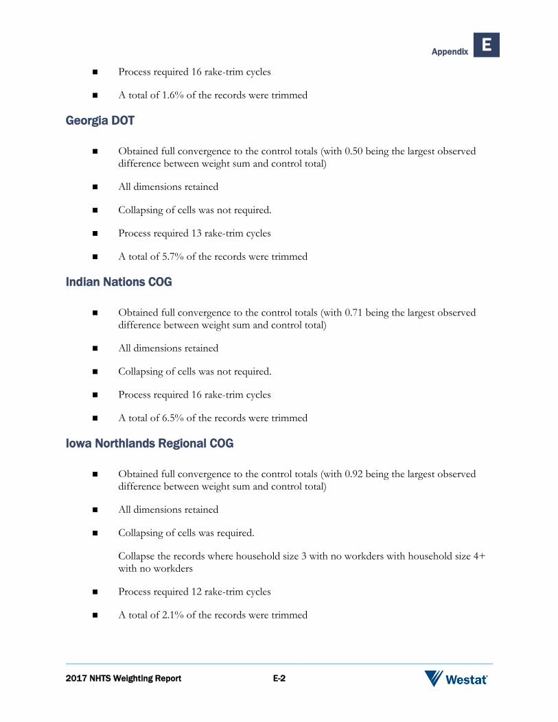
2017 NHTS Weighting Report E-2
Appendix E
Process required 16 rake-trim cycles
A total of 1.6% of the records were trimmed
Georgia DOT
Obtained full convergence to the control totals (with 0.50 being the largest observed difference between weight sum and control total)
All dimensions retained
Collapsing of cells was not required.
Process required 13 rake-trim cycles
A total of 5.7% of the records were trimmed
Indian Nations COG
Obtained full convergence to the control totals (with 0.71 being the largest observed difference between weight sum and control total)
All dimensions retained
Collapsing of cells was not required.
Process required 16 rake-trim cycles
A total of 6.5% of the records were trimmed
Iowa Northlands Regional COG
Obtained full convergence to the control totals (with 0.92 being the largest observed difference between weight sum and control total)
All dimensions retained
Collapsing of cells was required.
Collapse the records where household size 3 with no workders with household size 4+ with no workders
Process required 12 rake-trim cycles
A total of 2.1% of the records were trimmed
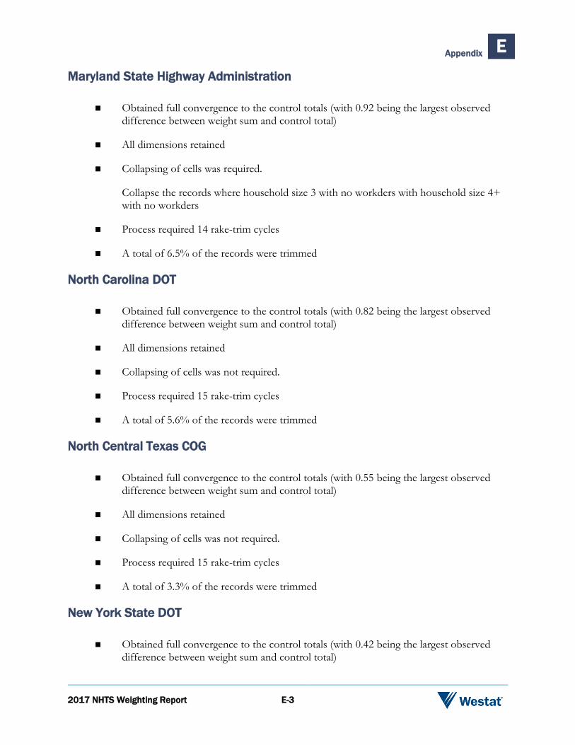
2017 NHTS Weighting Report E-3
Appendix E
Maryland State Highway Administration
Obtained full convergence to the control totals (with 0.92 being the largest observed difference between weight sum and control total)
All dimensions retained
Collapsing of cells was required.
Collapse the records where household size 3 with no workders with household size 4+ with no workders
Process required 14 rake-trim cycles
A total of 6.5% of the records were trimmed
North Carolina DOT
Obtained full convergence to the control totals (with 0.82 being the largest observed difference between weight sum and control total)
All dimensions retained
Collapsing of cells was not required.
Process required 15 rake-trim cycles
A total of 5.6% of the records were trimmed
North Central Texas COG
Obtained full convergence to the control totals (with 0.55 being the largest observed difference between weight sum and control total)
All dimensions retained
Collapsing of cells was not required.
Process required 15 rake-trim cycles
A total of 3.3% of the records were trimmed
New York State DOT
Obtained full convergence to the control totals (with 0.42 being the largest observed difference between weight sum and control total)

2017 NHTS Weighting Report E-4
Appendix E
All dimensions retained
Collapsing of cells was not required.
Process required 15 rake-trim cycles
A total of 6.4% of the records were trimmed
South Carolina DOT
Obtained full convergence to the control totals (with 0.49 being the largest observed difference between weight sum and control total)
All dimensions retained
Collapsing of cells was not required.
Process required 14 rake-trim cycles
A total of 6.0% of the records were trimmed
Texas DOT
Obtained full convergence to the control totals (with 0.56 being the largest observed difference between weight sum and control total)
All dimensions retained
Collapsing of cells was not required.
Process required 14 rake-trim cycles
A total of 4.5% of the records were trimmed
Wisconsin DOT
Obtained full convergence to the control totals (with 0.46 being the largest observed difference between weight sum and control total)
All dimensions retained
Collapsing of cells was not required.
Process required 16 rake-trim cycles
A total of 3.6% of the records were trimmed

2017 NHTS Weighting Report E-5
Appendix E
Census Division 1
Obtained full convergence to the control totals (with 0.83 being the largest observed difference between weight sum and control total)
All dimensions retained
Collapsing of cells was not required.
Process required 17 rake-trim cycles
A total of 7.4% of the records were trimmed
Census Division 2, excluding NY
Obtained full convergence to the control totals (with 0.44 being the largest observed difference between weight sum and control total)
All dimensions retained
Collapsing of cells was required.
Collapse the records where household size 3 with no workders with household size 4+ with no workders
Process required 17 rake-trim cycles
A total of 2.6% of the records were trimmed
Census Division 3, excluding WI
Obtained full convergence to the control totals (with 0.51 being the largest observed difference between weight sum and control total)
All dimensions retained
Collapsing of cells was not required.
Process required 17 rake-trim cycles
A total of 1.5% of the records were trimmed
Census Division 4, excluding IA Add-on areas
Obtained full convergence to the control totals (with 0.95 being the largest observed difference between weight sum and control total)

2017 NHTS Weighting Report E-6
Appendix E
All dimensions retained
Collapsing of cells was required.
Collapse the records where household size 3 with no workders with household size 4+ with no workders
Process required 16 rake-trim cycles
A total of 6.2% of the records were trimmed
Census Division 5, excluding GA, MD, NC, SC
Obtained full convergence to the control totals (with 0.53 being the largest observed difference between weight sum and control total)
All dimensions retained
Collapsing of cells was not required.
Process required 16 rake-trim cycles
A total of 5.7% of the records were trimmed
Census Division 6
Obtained full convergence to the control totals (with 0.59 being the largest observed difference between weight sum and control total)
All dimensions retained
Collapsing of cells was not required.
Process required 16 rake-trim cycles
A total of 0.8% of the records were trimmed
Census Division 7, excluding TX and Indian Nations Add-on area
Obtained full convergence to the control totals (with 0.51 being the largest observed difference between weight sum and control total)
All dimensions retained
Collapsing of cells was required.
Collapse the records where household size 3 with no workders with household size 4+ with no workders

2017 NHTS Weighting Report E-7
Appendix E
Process required 16 rake-trim cycles
A total of 3.4% of the records were trimmed
Census Division 8, excluding AZ
Obtained full convergence to the control totals (with 0.95 being the largest observed difference between weight sum and control total)
All dimensions retained
Collapsing of cells was not required.
Process required 15 rake-trim cycles
A total of 6.5% of the records were trimmed
Census Division 9, excluding CA
Obtained full convergence to the control totals (with 0.82 being the largest observed difference between weight sum and control total)
All dimensions retained
Collapsing of cells was not required.
Process required 16 rake-trim cycles
A total of 5.8% of the records were trimmed
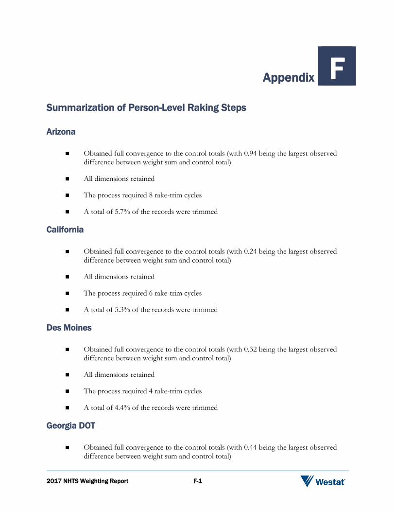
2017 NHTS Weighting Report F-1
Summarization of Person-Level Raking Steps
Arizona
Obtained full convergence to the control totals (with 0.94 being the largest observed difference between weight sum and control total)
All dimensions retained
The process required 8 rake-trim cycles
A total of 5.7% of the records were trimmed
California
Obtained full convergence to the control totals (with 0.24 being the largest observed difference between weight sum and control total)
All dimensions retained
The process required 6 rake-trim cycles
A total of 5.3% of the records were trimmed
Des Moines
Obtained full convergence to the control totals (with 0.32 being the largest observed difference between weight sum and control total)
All dimensions retained
The process required 4 rake-trim cycles
A total of 4.4% of the records were trimmed
Georgia DOT
Obtained full convergence to the control totals (with 0.44 being the largest observed difference between weight sum and control total)
Appendix F

2017 NHTS Weighting Report F-2
Appendix F
All dimensions retained
The process required 6 rake-trim cycles
A total of 5.4% of the records were trimmed
Indian Nations COG
Obtained full convergence to the control totals (with 0.73 being the largest observed difference between weight sum and control total)
All dimensions retained
The process required 5 rake-trim cycles
A total of 5.6% of the records were trimmed
Iowa Northlands Regional COG
Obtained full convergence to the control totals (with 0.47 being the largest observed difference between weight sum and control total)
All dimensions retained
The process required 5 rake-trim cycles
A total of 5.6% of the records were trimmed
Maryland State Highway Administration
Obtained full convergence to the control totals (with 0.38 being the largest observed difference between weight sum and control total)
All dimensions retained
The process required 6 rake-trim cycles
A total of 5.9% of the records were trimmed
North Carolina DOT
Obtained full convergence to the control totals (with 0.07 being the largest observed difference between weight sum and control total)
All dimensions retained
The process required 6 rake-trim cycles
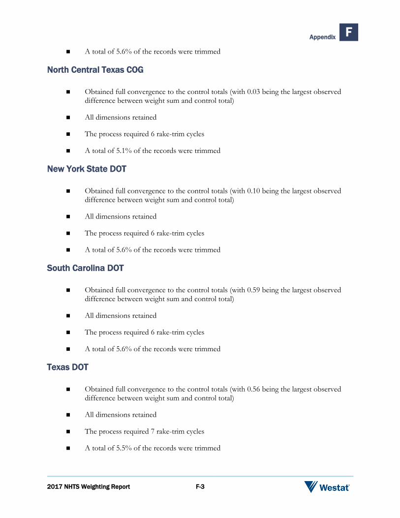
2017 NHTS Weighting Report F-3
Appendix F
A total of 5.6% of the records were trimmed
North Central Texas COG
Obtained full convergence to the control totals (with 0.03 being the largest observed difference between weight sum and control total)
All dimensions retained
The process required 6 rake-trim cycles
A total of 5.1% of the records were trimmed
New York State DOT
Obtained full convergence to the control totals (with 0.10 being the largest observed difference between weight sum and control total)
All dimensions retained
The process required 6 rake-trim cycles
A total of 5.6% of the records were trimmed
South Carolina DOT
Obtained full convergence to the control totals (with 0.59 being the largest observed difference between weight sum and control total)
All dimensions retained
The process required 6 rake-trim cycles
A total of 5.6% of the records were trimmed
Texas DOT
Obtained full convergence to the control totals (with 0.56 being the largest observed difference between weight sum and control total)
All dimensions retained
The process required 7 rake-trim cycles
A total of 5.5% of the records were trimmed

2017 NHTS Weighting Report F-4
Appendix F
Wisconsin DOT
Obtained full convergence to the control totals (with 0.60 being the largest observed difference between weight sum and control total)
All dimensions retained
The process required 6 rake-trim cycles
A total of 5.0% of the records were trimmed
Census Division 1
Obtained full convergence to the control totals (with 0.09 being the largest observed difference between weight sum and control total)
All dimensions retained
The process required 6 rake-trim cycles
A total of 5.6% of the records were trimmed
Census Division 2, excluding NY
Obtained full convergence to the control totals (with 0.62 being the largest observed difference between weight sum and control total)
All dimensions retained
The process required 5 rake-trim cycles
A total of 2.2% of the records were trimmed
Census Division 3, excluding WI
Obtained full convergence to the control totals (with 0.76 being the largest observed difference between weight sum and control total)
All dimensions retained
The process required 7 rake-trim cycles
A total of 2.8% of the records were trimmed
2017 NHTS Weighting Report F-5
Appendix F
Census Division 4, excluding IA Add-on areas
Obtained full convergence to the control totals (with 0.68 being the largest observed difference between weight sum and control total)
All dimensions retained
The process required 6 rake-trim cycles
A total of 5.9% of the records were trimmed
Census Division 5, excluding GA, MD, NC, SC
Obtained full convergence to the control totals (with 0.20 being the largest observed difference between weight sum and control total)
All dimensions retained
The process required 6 rake-trim cycles
A total of 5.6% of the records were trimmed
Census Division 6
Obtained full convergence to the control totals (with 0.06 being the largest observed difference between weight sum and control total)
All dimensions retained
The process required 7 rake-trim cycles
A total of 2.0% of the records were trimmed
Census Division 7, excluding TX and Indian Nations Add-on area
Obtained full convergence to the control totals (with 0.30 being the largest observed difference between weight sum and control total)
All dimensions retained
The process required 8 rake-trim cycles
A total of 5.6% of the records were trimmed
2017 NHTS Weighting Report F-6
Appendix F
Census Division 8, excluding AZ
Obtained full convergence to the control totals (with 0.33 being the largest observed difference between weight sum and control total)
All dimensions retained
The process required 6 rake-trim cycles
A total of 5.7% of the records were trimmed
Census Division 9, excluding CA
Obtained full convergence to the control totals (with 0.28 being the largest observed difference between weight sum and control total)
All dimensions retained
The process required 6 rake-trim cycles
A total of 5.6% of the records were trimmed