n.h.reyes@massey.ac.nz

D* Litean incremental version of A*

for navigating in unknown terrainIt implements the same behavior as Stentz’ Focussed Dynamic A* but is algorithmically different.

n.h.reyes@massey.ac.nz

Mars Rover

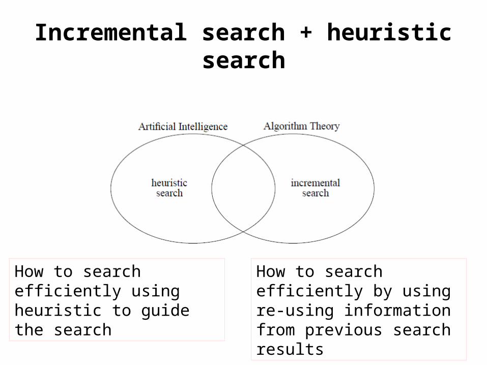
How to search efficiently using heuristic to guide the search

How to search efficiently by using re-using information from previous search results

Incremental search + heuristic search

• Stentz 1995• Clever heuristic method that achieves a speedup of one to

two orders of magnitudes over repeated A* searches• The improvement is achieved by modifying previous search

results locally• Extensively used on real robots, including outdoor high

mobility multi-wheeled vehicle (HMMWV)• Integrated into Mars Rover prototypes and tactical mobile

robot prototypes for urban reconnaissance

Focussed Dynamic A* (D*)

• D* Lite implements the same navigation strategy as D*, but is algorithmically different

• Substantially shorter than D*• Uses only one tie-breaking criterion when comparing

priorities (simplified maintenance)• No nested if statements with complex conditions• Simplifies the analysis of program flow• Easier to extend• At least as efficient as D*

D* Lite vs. D*

Previously, we learned LPA*

original eight-connected gridworld

LPA* repeatedly determines shortest paths between Sstart and Sgoal as the edge costs of a graph change.

Path Planning

original eight-connected gridworld

LPA* repeatedly determines shortest paths between Sstart and Sgoal as the edge costs of a graph change.

Path Planning

changed eight-connected gridworld

LPA* repeatedly determines shortest paths between Sstart and Sgoal as the edge costs of a graph change.

Path Planning

changed eight-connected gridworld

LPA* repeatedly determines shortest paths between Sstart and Sgoal as the edge costs of a graph change.

LPA*

• LPA* is an incremental version of A* that applies to the same finite path-planning problems as A*.

• It shares with A* the fact that it uses non-negative and consistent heuristics h(s) that approximate the goal distances of the vertices s to focus its search.

• Consistent heuristics obey the triangle inequality:– h(sgoal) = 0 – h(s) ≤ c(s, s’) + h(s’); for all vertices s ∈ S and

s’ ∈ succ(s) with s ≠ sgoal.

D* LiteLPA* repeatedly determines shortest paths between Sstart and Sgoal as the edge costs of a graph change.

D* Lite repeatedly determines shortest paths between the current vertex Scurrent of the robot and Sgoal as the edge costs of a graph

change, while the robot moves towards Sgoal.

D* LiteLPA* repeatedly determines shortest paths between Sstart and Sgoal as the edge costs of a graph change.

D* Lite repeatedly determines shortest paths between the current vertex Scurrent of the robot and Sgoal as the edge costs of a graph

change, while the robot moves towards Sgoal.

D* Lite is suitable for solving goal-directed navigation problems in unknown terrains.

Free space Assumption

Free space Assumption

Free space assumptionMove the robot on a shortest potentially unblocked path towards the goal.

Using the free space assumption in path planning

Search from the Goal towards the robot’s current location- This allows one to re-use parts of the search tree after the

robot has moved.- This allows one to use heuristics to focus the search; thereby

not requiring to search the entire graph.

Using the free space assumption in path planning

Search from the Goal towards the robot’s current location- This makes incremental search efficient.

Variables

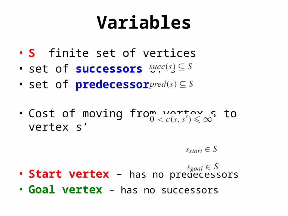
• S finite set of vertices• set of successors of s• set of predecessors of s • Cost of moving from vertex s to vertex s’

• Start vertex – has no predecessors

• Goal vertex – has no successors

LPA* Variables• Start distance = length of the shortest path

from Sstart to S

• g(s) = estimate of the Start distance g*(s)

D* Lite Variables• Goal distance = length of the shortest path

from S to Sgoal

• g(s) = estimate of the Goal distance g*(s)

LPA* Rhs-valueThe rhs-values are one-step look-ahead values, based on the g-values; and thus, potentially better informed than the g-values

D* Lite Rhs-valueThe rhs-values are one-step look-ahead values, based on the g-values; and thus, potentially better informed than the g-values

D* Lite Rhs-value

• g-value = rhs-value: cell is locally consistent• g-value ≠ rhs-value: cell is locally inconsistent• g-value > rhs-value: cell is locally overconsistent• g-value < rhs-value: cell is locally underconsistent

• the priority queue contains exactly the locally inconsistent vertices • their priority is [min(g(s),rhs(s)) + h(s,sstart) + km; min(g(s),rhs(s))]• smaller priorities first, according to a lexicographic ordering

The rhs-values are one-step look-ahead values, based on the g-values and thus potentially better informed than the g-values

Shortest Path• If all vertices are locally consistent,

– g(s) == g*(s) ; for all vertices s– one can trace back the shortest path from Sstart to Sgoal.

• From vertex s, find a successor s’ that minimises g(s’) + c(s, s’). • Ties can be broken arbitrarily.• Repeat until Sgoal is reached.

from Sstart to Sgoal

Selective Update• D*Lite does not make all vertices locally consistent

after some edge costs have changed• It uses heuristics to focus the search• It updates only the g-values that are relevant for

computing the shortest path

Priority• D*Lite maintains a priority queue for keeping track of

locally inconsistent vertices – vertices that potentially needs their g-values updated to make them locally consistent

• Priority of a vertex = key• Key – vector with 2 components

k(s) = [ k1(s); k2(s) ]

k1(s) = min(g(s), rhs(s)) + h(s, sstart) + km

k2(s) = min(g(s), rhs(s))

Priority• Priority of a vertex = key• Key – vector with 2 components

k(s) = [ k1(s); k2(s) ]

k1(s) = min(g(s), rhs(s)) + + h(s, sstart) + km

k2(s) = min(g(s), rhs(s))

Key comparison (lexicographic ordering): k(s) ≤ k’(s) iff either ( k1(s) < k1‘(s) )

or ( k1(s) == k1‘(s) ) and

( k2(s) ≤ k2‘(s) )

The vertex with the smallest key is

expanded first by D*Lite.

Heuristic Function (8-connected Gridworld)

• As an approximation of the distance between two cells, we use the maximum of the absolute differences of their x and y coordinates.

• These heuristics are for eight-connected gridworlds what Manhattan distances are for four-connected gridworlds.

Lifelong Planning A* h(s, sgoal) – calculated relative to the goal position

D*Lite h(s, sstart) – calculated relative to the start position

The pseudocode uses the following functions to manage the priority queue:

• U.TopKey() - returns the smallest priority of all vertices in priority queue U.

(If U is empty, then U.TopKey() returns [∞; ∞].) • U.Pop() - deletes the vertex with the smallest priority in priority

queue U and returns the vertex. • U.Insert(s; k) - inserts vertex s into priority queue U with priority k.• Update(s; k) - changes the priority of vertex s in priority queue U to

k. (It does nothing if the current priority of vertex s already equals k.)

• U.Remove(s) - removes vertex s from priority queue U.

Priority Queue Management

LPA* Pseudocode (just for comparison)

D* Lite Pseudocode

gets satisfied when one of the edge costs change

Route-planning example: 4-connected gridworld

Example, Step 1

Route-planning example: 4-connected gridworld

Example, Step 2

Route-planning example: 4-connected gridworld

Example, Step 3

Route-planning example: 4-connected gridworld

Example, Step 4

Route-planning example: 4-connected gridworld

Example, Step 5

After one cell gets blocked…

Blocked cell: C3

The previous search results are carried over to help solve this re-planning problem.

After one cell gets blocked…

Blocked cell: C3

Neighbours of C3: B3, C4, D3, C2

Among the neighbours, Cells B3 & C2 calculates their rhs-values based on C3; therefore, set their g-values to ∞

Route-planning example: 4-connected gridworld

Example, Step 6

Route-planning example: 4-connected gridworld

Example, Step 7

Route-planning example: 4-connected gridworld

Example, Step 8

Route-planning example: 4-connected gridworld

Example, Step 9

Route-planning example: 4-connected gridworld

Example, Step 10

Route-planning example: 4-connected gridworld

Example, Step 11

Route-planning example: 4-connected gridworld

Example, Step 12

Simulation Example

D* Lite operating in a 4-Connected Gridworld

demonstration of the use of the km variable

Route-planning example #2: 4-connected gridworld

Example, Step 1

Route-planning example #2: 4-connected gridworld

Example, Step 2

Route-planning example #2: 4-connected gridworld

Example, Step 3

Route-planning example #2: 4-connected gridworld

Example, Step 4

Route-planning example #2: 4-connected gridworld

Example, Step 5

Cell C3 gets blocked…

Route-planning example #2: 4-connected gridworld

Example, Step 6

Route-planning example #2: 4-connected gridworld

Example, Step 7

Route-planning example #2: 4-connected gridworld

Example, Step 8

Route-planning example #2: 4-connected gridworld

Example, Step 9

Route-planning example #2: 4-connected gridworld

Example, Step 10

Route-planning example #2: 4-connected gridworld

Example, Step 11

Route-planning example #2: 4-connected gridworld

Example, Step 12

Route-planning example #2: 4-connected gridworld

Example, Step 13

Route-planning example #2: 4-connected gridworld

Example, Step 14

Route-planning example #2: 4-connected gridworld

Example, Step 15

Route-planning example #2: 4-connected gridworld

Example, Step 16

Conclusions

• D* Lite is a fast re-planning method for robot navigation in unknown terrain.

• It implements the same navigation strategies as D*, and is at least as efficient as D*.

References• http://idm-lab.org/publications.html• http://idm-lab.org/project-a.html• http://homepages.dcc.ufmg.br/~lhrios/applet_d_lite/index.html• A complete navigation system for goal acquisition in unknown

environments, Anthony Stentz and Martial Hebert