nhf local economic impacts calculator (leic)

NHF Local Economic Impacts Calculator (LEIC):

Methodology and assumptions March 2020

2

© Centre for Economics and Business Research

Disclaimer

Whilst every effort has been made to ensure the accuracy of the material in this document, neither Centre for Economics and

Business Research Ltd. nor the report’s authors will be liable for any loss or damages incurred through the use of the report.

Authorship and acknowledgements

This report has been produced by Cebr, an independent economics and business research consultancy established in 1992. The

views expressed herein are those of the authors only and are based upon independent research by them.

The report does not necessarily reflect the views of NHF.

London, March 2020

3


Contents

1 Introduction 4

2 Key aspects of the underlying methodology 5

3 Economic impact of Housing Associations 7

4 Economic impact of HA investments in new affordable homes 10

5 Application of the modelling framework 14

5.1 Completing the embedding process 14

5.2 Multiplier impacts based on Leontief input-output framework 15

5.3 Regional multiplier impacts based on location quotients 15

6 The multiplier results 17

Appendix: PREVIOUS multiplier results (2010 basis) 19

4


1 Introduction This is a statement of the methodologies and assumptions underlying the Local Economic Impacts Calculator that Cebr first constructed in 2012 on behalf of the National Housing Federation.

The point of the LEIC is to allow users (NHF housing association members) to estimate the economic impacts of their:

a investments in new affordable housing; and

b day-to-day activities in managing their existing stocks of housing.

Originally, the database provided impacts at the regional, national and UK level. In 2014, the model was innovated to include a tool that could be used to estimate these impacts at the local authority (LA) and local enterprise partnership (LEP) level.

The LEIC produces impacts at the LA level that are derived on the basis of the HA user’s estimates of the proportion of the different elements of their supply chain that are provided by people or businesses located within the LA or LEP. The higher the percentage of housing investment, for example, that is supported by local goods and services, the greater the likelihood that the multiplier impacts of this investment will be realised within the locality. But it is important to note that goods and services that are not supplied within the local economy are likely to be supplied from other local authority areas, generating multiplier impacts in other parts of the UK.

The 2016 update of the LEIC built in the ability to estimate impacts at the Combined Authority (CA) level. Five CAs were incorporated in 2016. The 2017 update incorporated a further four CAs, including two options for the West Midlands CA – one including constituent LAs only and one including constituents and non-constituents (which we understand to be candidates for inclusion).

The May 2018 refresh of the LEIC was updated to incorporate changes in the make-up of the combined authorities, including the removal of the North East CA and the addition of the new North of Tyne CA and changes in the local authority compositions of some of the others. It also reflects the merging of Northamptonshire LEP with South East Midlands LEP to create the "NEW South East Midlands LEP" featured in the database.

The April 2019 iteration incorporated minor changes, principally the inclusion of five new Local Authorities within the Sheffield City Region CA and the name change for the Shepway LAD to Folkestone & Hythe. This latter change was then fully embedded into this year’s update. The 2019 update to the LEIC also continued to incorporate the 2018 migration to Cebr’s updated input-output models. Up to then, these models and the estimates of the multiplier impacts they produce, were based on 2010 ONS input-output data. The new models are based on 2013 input-output data.

The principal structural change reflected in this March 2020 update is the creation of five new Unitary Authorities. These are East Suffolk (previously Suffolk Coastal and Waveney); West Suffolk (previously Forest Heath and St. Edmundsbury); Bournemouth, Christchurch & Poole (previously three separate local authorities); Dorset Council (previously East Dorset, North Dorset, Purbeck, Weymouth & Portland and West Dorset) and Somerset West & Taunton (previously Taunton Deane and West Somerset). The new Unitary Authorities have been fully incorporated into Worksheets 3 and 4 and partially incorporated into Worksheet 5. As the raw datasets become consistent these changes will also be fully incorporated into this worksheet.

5


2 Key aspects of the underlying methodology

To estimate the impacts of investments by HAs in affordable housing or of HAs’ day-to-day activities, it is necessary to combine national statistics and the economic data on affordable housing and housing associations that could be accessed in the public domain or that could be provided by NHF through the data it collects from its member HAs.

The modelling framework starts with the ONS’ supply-use tables, the most detailed official record of how the industries of the economy interact with other industries, with consumers and with international markets in producing the nation’s GDP and national income. The purpose of the supply-use tables is to reconcile the three approaches to estimating GDP – the production approach, the income approach and the expenditure approach.

Making use of the supply-and-use framework to analyse HA investments in new affordable homes and HA day-to-day activities – which are only subsets of industries at the level of disaggregation provided by this framework – is the best means of ensuring consistency with the national accounts. The process of embedding the specific subsets of activities within this framework involves assigning them explicit roles within the supply-use tables.

Having assigned roles within the supply-use framework for each of the relevant activities of housing associations – new affordable homes investments and day-to-day management of existing stock – we had the foundation for establishing, through our input-output models:

The economic size (or direct impact) of both activities using standard measures of GVA1 contributions to GDP, of contributions to employment and to employee compensation; and

The wider economic impact of both activities on the UK economy, using Leontief input-output modelling to estimate a full set of (matrix) multipliers capturing direct, indirect and induced impacts on output, GVA, employment and employee income.

The multipliers capture indirect impacts on production in the economy through the supply chain response to the demands of HAs in supporting their investments in new affordable homes and their day-to-day activities, and induced impacts on production when the direct and indirect employees of HAs spend their earnings in the wider economy on the final consumption goods and services required by households.2

The input-output model produces multipliers in the form of pound-for-pound and job-for-job ratios between total and direct impacts. These are used in association with the direct impacts data to produce

1 GVA or gross value added is a measure of the net value of goods and services which, in the national accounts, is the value of

industrial output less intermediate consumption. That is, the value of what is produced less the value of the intermediate goods and services used as inputs to produce it. GVA is also commonly known as income from production and is distributed in three directions – to employees, to shareholders and to government. GVA is linked as a measurement to GDP – both being a measure of economic output. That relationship is (GVA + Taxes on products - Subsidies on products = GDP). Because taxes and subsidies on individual product categories are only available at the whole economy level, GVA tends to be used for measuring things like gross regional domestic product and other measures of economic output of entities that are smaller than the whole economy, such as Housing Associations. 2 Note that a Type I matrix multiplier captures direct and indirect impacts, whilst the Type II includes direct, indirect and induced

impacts.

6


estimates of the absolute magnitudes of the total economic ‘footprint’ of HA affordable homes investment and day-to-day activities.

7


3 Economic impact of Housing Associations

This section provides the methodology and assumptions underlying Worksheet 4: Impacts of Housing Associations’ Day-to-Day Activities in the LEIC. This allows LEIC users to estimate the economic impacts of their day-to-day activities in managing their existing stock of housing.

The process of assigning HAs’ day-to-day activities (incl. repair and maintenance) an explicit role within the supply-use tables requires, as a starting point, estimates of the relevant economic indicators from the aggregate financial data that exists covering those activities. These were sourced from the Global Accounts for housing associations compiled by the Homes and Communities Agency (HCA), and formerly the Tenant Services Authority (TSA). The HCA global accounts provide income and expenditure data, including revenue grants received, relating to HA day-to-day activity.

NHF provides turnover and employment data at the regional level, which informs the regional analysis of HAs’ day-to-day activities.

Building a picture of size and structure of HAs’ supply chains – fundamental to understanding economic impacts – was helped by the aggregate estimates from the aforementioned sources but also, to an extent, by the expenditure breakdowns provided within them. However, gaps remained, in which case we developed assumptions based on the data for the broader sector of which HAs form part (real estate services).

Taking the total turnover of HAs as, in economic terms, the total demand for their services provides the starting point. This is followed by a process of backward induction through the supply-use tables, involving:

matching the demand for HA services to their supply;

establishing the corresponding national production, income and expenditure accounts for HAs, including the structure of HAs’ supply chain;

adjusting the supply-use tables to ensure that they are re-balanced to GDP under the production, income and expenditure approaches to its calculation.

The Global Accounts suggest that the total turnover of housing associations is as presented in Table 1 below, on both a “consolidated” and “entity” basis.

Table 1: Total turnover of Housing Associations, £millions

Year Housing Associations' Aggregate

Turnover £m (Cons) Housing Associations' Aggregate

Turnover (Entity) £m

2015 £16,268

2016 £17,787

2017 £19,997 £17,987

2018 £20,459 £18,383

2019 £20,860 £18,704

Source: HCA Global accounts 2015-2019

The 2020 version of the LEIC is based on local-level numbers that reconcile to most of the “entity” 2019 estimate of £18,704 million. Specifically, the local-level numbers sum to £18,528 million (£18,523 million

8


for England only). Previous iterations have also been based on local numbers that sum to amounts closer to the “entity” estimates. The only exception is the 2019 LEIC, for which Cebr was supplied local-level numbers closer to the 2018 “cons” estimate.

The process of embedding HAs’ economic activities within the supply-use and input-output models required estimates of several other economic indicators. Values for these indicators were estimated based on the data from the sources previously outlined. These are detailed as follows:

1. Taxes less subsidies on production: this consists of business rates and employers’ national insurance contributions (NICs) at a minimum, sourced from the HCA Global Accounts.

2. Employment: headcount numbers derived by NHF from the HCA Global Accounts.3

3. Compensation of employees: HAs’ people costs are based on these same headcount numbers, which are combined with data on employment profiles and wages obtained from the ONS.

4. Gross operating surplus and mixed income: this includes any HA operating surplus, sourced from the HCA global accounts, including allowances for the depreciation of property and other assets.

5. Intermediate consumption (supply chain): spend by HAs on externally sourced intermediate inputs, including from other HAs or other real estate service providers.

Table 2 below shows our estimates of the size and structure of the supply chains associated with housing associations’ day-to-day activities.

The table shows the categories of externally sourced intermediate goods and services that HAs require to carry out their own activities and, therefore, the industries from which they purchase them. It is in these industries that jobs and economic output are supported by the day-to-day activities of housing associations at the local, regional and national level.

By far the greatest proportion of HAs’ external spend is in the construction sector. This reflects expenditures on repair and maintenance of existing housing stocks (anything from plumbing or electrical repairs to significant improvements to the property). The next highest expenditures are estimated to be in finance and insurance – 7.1 per cent – and information and communications – 2.6 per cent.

3 Previously, we used estimates from the ONS regarding the full-time and part-time split of employment to show HA

employment on a full-time equivalent (FTE) basis. However, this is arguably a superfluous step that only renders the LEIC unnecessarily inaccurate. Furthermore, given wider developments in the labour market, we have moved our new supply-use and input-output models away from using FTEs to using ‘people in jobs’ instead.

9


Table 2: Structure of HAs’ supply chain supporting their day-to-day activities, % of total

Sector Percentage of

Total

Construction 80.3%

Financial and Insurance Activities 7.1%

Information and Communication 2.6%

Manufacturing 2.4%

Real Estate Activities 1.7%

Administrative and Support Service Activities 1.5%

Housing Associations (day to day) 1.3%

Professional, Scientific and Technical Activities 1.2%

Transport and Storage 0.8%

Education 0.4%

Accommodation and Food Service Activities 0.3%

Water Supply, Sewerage and Waste Management 0.2%

Electricity, Gas, Steam and Air Conditioning supply 0.2%

Source: NHF, HCA, ONS, Cebr analysis

10


4 Economic impact of HA investments in new affordable homes

This section provides the methodology and assumptions underlying Worksheet 3: Impacts of Affordable Homes Investment in the LEIC. This allows LEIC users to estimate the economic impacts of their investments in new affordable housing.

The process of estimating these impacts is much the same as for estimating the impacts of HAs’ day-to-day activities, as described above. But there are some important differences, as outlined here. For affordable housing investment, the relevant economic indicators are estimated from several sources, including:

Investment expenditure, both per home and in total, under the Shared Ownership and Affordable Homes Programme (SOAHP 4 ), the Affordable Homes Programmes (AHPs 5 ) and the National Affordable Housing Programme (NAHP6), provided by NHF through the HCA, but also based on data from National Audit Office (NAO); and

Data provided by NHF housing association members regarding the breakdown of expenditure for numerous affordable housing investment projects under the NAHP.

Unlike in the case of housing associations, where the direct economic impact of their day-to-day activities comes through the housing associations themselves, in the case of investment expenditure, the direct economic impact is felt through the industries that benefit from the investment expenditures made by the housing associations. These are commonly referred to as the ‘beneficiary’ industries – those that supply the capital inputs required to build new affordable homes. By establishing the share of output of these industries that is due to investment in affordable homes, we had the starting point for embedding the activities stimulated by this investment within the same supply-use and input-output modelling framework.

The aforementioned data sources suggest that the total expenditure on affordable housing investment under the current 2016-2021 SOAHP is as presented in Table 3 below. This includes an average measure of total scheme cost per home delivered.

This TSC per home measure is an important input underlying this part of the LEIC. Along with the number of homes involved in the scheme, as inputted by users of the LEIC, the TSC per home measure provides the starting point for determining the economic impacts of any new affordable housing investments.

4 Running from 2016 to 2021. 5 The first Affordable Homes Programme (AHP) ran between 2011 and 2015, delivering an estimated 186,000 affordable homes

in total. The new AHP runs from 2015 to 2018. 6 The National Affordable Housing Programme (NAHP) ran between 2008 and 2011, delivering an estimated 155,000 new

homes.

11


Table 3: 2016-21 SOAHP total scheme costs (TSC) by HCA operating area (end September 2019)

HCA Operating Area TSC Homes TSC/home

Midlands £2,179,266,520 14,957 £145,702

North East / Yorkshire & Humber £1,806,151,661 1,334 £135,455

North West £2,488,483,885 17,183 £144,822

South East £5,703,382,183 28,869 £197,561

South West £2,931,121,876 15,980 £183,424

Total £15,108,406,125 90,323 £167,271

Source: Homes England (2020)

The TSC per home measure for London is £278,000, based on data provided by the Greater London Authority, which is responsible for funding and delivering the AHP in London.7

Only the construction costs and the on-costs of any scheme are taken forward in the analysis. This is because land purchases are not a value-generating economic activity, rather a simple transfer of wealth or capital. For this reason, Table 4 presents the estimates of how total scheme costs are broken down between land, construction and on-costs for affordable housing schemes in each of the English regions. The construction cost percentages in this NAHP-based table broadly correspond with the “Works Cost” shares for the latest 2016-2021 SOAHP release.

Table 4: Breakdown of total scheme costs by land, construction and on-cost

HCA Operating Area Land Construction On-Cost Construction + On-Cost

South East 21.0% 66.9% 12.0% 79.0%

East of England 19.5% 69.4% 11.2% 80.5%

London 30.6% 56.8% 12.6% 69.4%

East Midlands 23.9% 65.3% 10.8% 76.2%

West Midlands 23.4% 66.1% 10.5% 76.6%

Yorkshire and the Humber 20.1% 68.8% 11.1% 79.9%

North East 15.5% 74.7% 9.9% 84.5%

North West 17.0% 71.1% 11.9% 83.0%

South West 21.9% 66.7% 11.4% 78.1%

England 21.0% 67.0% 11.0% 78.0%

Source: Cebr analysis of schemes under NAHP

The data in Table 3 is scaled per these assumptions before entering the supply-use and input-output framework on which the impact workings within the LEIC are based.

7 This £278,000 average scheme cost for London is the figure calculated for the 2017 update of the LEIC. There are still no data

that would enable this figure to be updated for the current year.

12


Using investment project-specific data from housing associations (supplied to Cebr through NHF), we identify the ‘beneficiary’ industries of this investment spend. These are shown in Table 5 below.

Table 5 - Contribution to affordable housing investment by sector

Sector Percentage of

total

Construction 68.96%

Professional Scientific and Technical Activities 16.36%

Administrative and Support Service Activities 4.64%

Wholesale and Retail Trade, Repair of Motor Vehicles 3.74%

Water Supply, Sewerage and Waste Management 3.17%

Electricity, Gas, Steam and Air Conditioning supply 2.59%

Information and Communication 0.26%

Human Health and Social Work Activities 0.26%

Manufacturing 0.02%

Source: NHF, NAO, ONS, Cebr analysis

The next step was to undertake a similar process of embedding the relevant activities within the framework for analysis as described for HAs’ day-to-day activities, beginning with estimates of the other economic indicators required to complete that process. These were estimated based on data on the beneficiary industries in the supply-use tables but, in this process, the starting point is to establish an explicit role for the stimulus provided to the ‘beneficiary’ industries as a result of HA investments (as opposed to HA activities).

This included establishing a ‘composite’ supply chain for the beneficiary industries. Table 6 presents the structure of this composite supply chain of the industries that deliver the goods and services required to realise new investment in affordable homes.

13


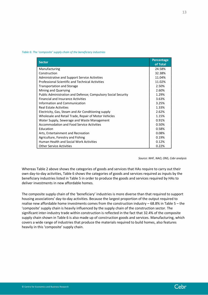
Table 6: The ‘composite’ supply chain of the beneficiary industries

Sector Percentage

of Total

Manufacturing 24.58% Construction 32.38% Administrative and Support Service Activities 11.04% Professional Scientific and Technical Activities 11.02% Transportation and Storage 2.50% Mining and Quarrying 2.60% Public Administration and Defence; Compulsory Social Security 1.29% Financial and Insurance Activities 3.63% Information and Communication 3.25% Real Estate Activities 1.33% Electricity, Gas, Steam and Air Conditioning supply 2.62% Wholesale and Retail Trade, Repair of Motor Vehicles 1.15% Water Supply, Sewerage and Waste Management 0.91% Accommodation and Food Service Activities 0.50% Education 0.58% Arts, Entertainment and Recreation 0.08% Agriculture, Forestry and Fishing 0.19% Human Health and Social Work Activities 0.12% Other Service Activities 0.22%

Source: NHF, NAO, ONS, Cebr analysis

Whereas Table 2 above shows the categories of goods and services that HAs require to carry out their own day-to-day activities, Table 6 shows the categories of goods and services required as inputs by the beneficiary industries listed in Table 5 in order to produce the goods and services required by HAs to deliver investments in new affordable homes.

The composite supply chain of the ‘beneficiary’ industries is more diverse than that required to support housing associations’ day-to-day activities. Because the largest proportion of the output required to realise new affordable home investments comes from the construction industry – 68.8% in Table 5 – the ‘composite’ supply chain is heavily influenced by the supply chain of the construction sector. The significant inter-industry trade within construction is reflected in the fact that 32.4% of the composite supply chain shown in Table 6 is also made up of construction goods and services. Manufacturing, which covers a wide range of industries that produce the materials required to build homes, also features heavily in this ‘composite’ supply chain.

14


5 Application of the modelling framework The estimates taken forward from the previous sections provide the basis for completing the embedding process for both housing associations’ day-to-day activities and the stimulus provided by investments in new affordable homes.

5.1 Completing the embedding process

This involves incorporating the estimates into an adapted version of the aggregate combined use matrix. This comes in three parts:

a) The intermediate demand part, showing the inputs of products (goods and services) – both domestic and imported, but not separately – used by UK industries in the production of their output.

b) The final demand part, showing the purchases of each product by each category of final demand in the UK – households (consumers), government, investment and exports.

c) The primary inputs part, showing payments to inputs that do not flow through the other industries but rather reflect employees’ salaries, taxes less subsidies on production and gross operating surplus and mixed income.8

The aggregate supply table incorporates taxes less subsidies on products, which are important for translating gross turnover (in the case of housing associations) and gross investment (in the case of new affordable homes) into measures of ‘industrial’ output, from which all economic contributions and impacts flow.

The primary inputs part (which corresponds with the income account) was completed for housing associations and for the ‘beneficiary’ industries from new affordable homes investments using a combination of the data supplied by the National Housing Federation, obtained from the HCA and the ONS and within the supply-use tables themselves (particularly for investment).

Completion of the intermediate demand and final demand parts of the combined use table, in the case of housing associations’ day-to-day activities, required an assumption about the final demand from households for housing associations’ services. We base this on income data from the HCA global accounts and the assumption that only 45 per cent9 of rental income accruing to housing associations is paid by tenants themselves, with the difference being funded by housing benefit payments made directly to housing associations.10

Having thus assigned explicit roles within the supply-use tables to (i) the day-to-day activities of housing associations and (ii) the subset of industries stimulated through affordable homes investment, we had the basis for assessing their direct economic impacts, in terms of GVA contributions to GDP, employment and employee compensation. These are calculated within the aggregate combined use table described above.

8 These three together constitute gross value added (GVA). 9 This assumption is based on the percentage reported by housing associations. See for example, ‘English housing associations:

Direct payment of benefit to tenants a manageable risk’. Moody’s investors service, 30 May 2012. 10 For details on the current payment of housing benefits and planned changes see ‘Paying Housing Benefit direct to tenants in

social rented housing’. House of Commons Library, 5 April 2012.

15


The embedding process and the direct impacts also provided the ingredients required to assess the indirect and induced multiplier impacts of both (i) and (ii) through incorporation within Cebr’s updated input-output models.

5.2 Multiplier impacts based on Leontief input-output framework

Multipliers show the ratio of an induced change in national income to an initial change in the level of final demand spending, where the multiplier effect denotes the phenomenon whereby some initial increase (or decrease) in the rate of spending will bring about a more than proportionate increase (or decrease) in national income. The Keynesian approach barely requires a mention but is very much grounded in macroeconomic analysis, offering little capability to analyse impacts of entities that are smaller than the whole economy.

Input-output analysis, due largely to the work of Wassily Leontief11, while macroeconomic in the sense that it involves analysing the economy as a whole, owes its foundations and techniques to the microeconomic analysis of production and consumption.12 According to ten Raa (2005), some people argue that input-output analysis is at the interface of both, defining it as the study of industries or sectors of the economy.

The well-known Leontief inverse matrix, which shows the inter-industry dependencies of an economy, is the basis for producing so-called ‘ordinary’ (or traditional) input-output multipliers. These are some of the most important tools for measuring the total impact on output, employment and income when there is a change in final demand.

The Leontief inverse matrix can also be described as the output requirements matrix for final demand, that is, it shows the input requirements from the other sectors of the economy per unit of output produced in the sector under examination in response to the demand stimulus provided by the relevant set of economic activities. The matrix can be used to produce two types of multiplier – the Type I multiplier incorporating direct and indirect (supply chain) impacts and the Type II multiplier incorporating induced (through higher incomes and resulting greater consumption) impacts as well.

Cebr’s baseline multiplier model is based on this Leontief input-output modelling approach. The model is based on a so-called ‘domestic use’ table, from which imports are extracted from intermediate demands in order to focus on the domestic economy impacts of the relevant set of economic activities.

5.3 Regional multiplier impacts based on location quotients

The starting point in determining the economic impacts of the activities under consideration in the regions was to allocate the attributable shares of those activities to those regions. We did this according to GVA using:

i. For housing association’s day-to-day activities, the share of aggregate housing association turnover attributable to each region from the HCA global accounts.

ii. For new affordable homes investments, the share of affordable housing built in each region, also based on data supplied by NHF through HCA.

11 See, for example, Leontief, Wassily W. Input-Output Economics. 2nd ed., New York: Oxford University Press, 1986. 12 See ten Raa, Thijs (2005), The Economics of Input-Output Analysis, Cambridge University Press.

16


The total GVA and employment impacts presented in the results sections for each of the English regions were obtained by first estimating the relevant regional multipliers.

The key issue with producing regional technical coefficients13 is that regional propensities to import tend to be higher than national propensities, meaning local borders are more porous than national frontiers. We captured this through the use of ‘location quotients’. Location quotients (LQ) involve adjusting the UK-wide technical coefficients to take account of differing proportions of local demands being satisfied locally. They are interpreted as a measure of the ability of a particular industry in a particular region to supply the demands placed upon it by other industries and by final demand in the region.

Under this interpretation, a LQ > 1 implies that the industry is more concentrated in the region than in the UK as a whole, while a LQ < 1 implies that the industry is less concentrated in the region than in the whole of the UK.14

However, these simple location quotients assume that the differences between the UK and regional/national technical coefficients are the same across the sectors. Therefore, to capture differences between the amounts of cross-industry trade at the regional / national level and the UK level, we used more advanced Cross-Industry Location Quotients (CILQ). CILQs take account of the relative sizes of the sectors providing and purchasing inputs.

Under this interpretation, a CILQ < 1 implies that the supplying sector is relatively small compared to the purchasing sector at the regional level, so some of the required inputs might need to be imported from elsewhere in the UK. A CILQ > 1 means there is no need to adjust the UK technical coefficients as all the needs for the input can likely be met from within the region.

The results of this analysis are unique matrices of technical coefficients for each of the regions. From these, the multiplier impacts of housing associations’ day-to-day activities and of new affordable homes investments in each of the regions are determined, using a modelling approach that takes account of the different underlying structures of these regional economies.

13 Technical co-efficients are also known as direct requirements and represent the amounts of intermediate consumption of the

various product/service categories from which the industry in question draws its inputs per £1 of output of that industry. 14 These ‘simple’ location quotients are calculated as a ratio of the share of the relevant sector in total regional GVA and the

share of the relevant sector in total UK GVA.

17


6 The multiplier results The multipliers are summarised in Table 7 and Table 8 below, which show the UK level Type I and Type II multipliers for affordable homes investment and housing associations’ day-to-day activities, respectively.

The interpretation of the multipliers, taking the GVA example, is that for every £1 of GVA generated by the beneficiary industries in delivering an affordable homes investment, an aggregate GVA impact of £2.36 is the outcome once indirect and induced multiplier impacts are accounted for. This is a £1.36 stimulus through the ‘composite’ supply chain of the beneficiary industries and through the spending of the direct and indirect employees of the beneficiary industries in the wider economy on the final goods and services required by households.

Table 7 - Affordable homes investment Type I and II UK level multipliers

New affordable homes Type I Type II

GVA 1.82 2.36

Output 1.78 2.23

Income 1.87 2.31

Employment 1.85 2.36

Likewise, the multipliers in Table 8Error! Reference source not found. can be interpreted in a similar fashion. Taking the GVA example again, for every £1 of GVA generated through the day-to day activities of housing associations, the aggregate GVA impact is £2.55 once the indirect and induced multiplier impacts are taken into account. This, again, is a £1.55 stimulus through the supply chains supporting HAs’ day-to-day activities and through the spending of the direct and indirect employees of housing associations in the wider economy on final goods and services.

Table 8 - Housing associations' day-to-day activities Type I and II UK level multipliers

HA day-to-day activities Type I Type II

GVA 1.98 2.55

Output 1.97 2.44

Income 1.92 2.47


The multipliers for England and the English regions are outlined in detail in Table 10 below.

It is not feasible to produce comprehensive sets of local-level multiplier impacts, but they can be expected to be some fraction of the UK and the relevant regional multipliers, depending on the extent to which housing associations and the beneficiary industries that help them deliver investments in new affordable homes import inputs from outside their local economy. The LEIC allows users to specify this as an input and, in producing local level impacts, adjusts the technical coefficients underlying the broader multiplier estimates to control for the non-local sourcing of inputs at the local economy level. (This is similarly the case when the LEP or Combined Authority is chosen as the geographic scope of the assessment.)

18


Table 9: Multipliers for England and the English regions

19


Appendix: PREVIOUS multiplier results (2010 basis) Affordable homes investment Type I and II UK level multipliers, 2010 basis

New affordable homes Type I Type II

GVA 1.93 2.42

Output 1.91 2.34

Income 2.03 2.45


Housing associations' day-to-day activities Type I and II UK level multipliers, 2010 basis

HA day-to-day activities Type I Type II

GVA 1.83 2.52

Output 1.81 2.42

Income 1.90 2.62


20


Table 10: Multipliers for England and the English regions, 2010 basis

nhf local economic impacts calculator (leic)

Documents