Network for Greening the Financial System

NGFS Climate Scenarios for central banks and supervisorsJune 2020

NGFS SCENARIOS 2

The Network for Greening the Financial System (NGFS) is a group of 66 central banks and supervisors and 13 observers committed to sharing best practices, contributing to the development of climate and environment‑related risk management in the financial sector and mobilising mainstream finance to support the transition towards a sustainable economy.

The NGFS Climate Scenarios were produced over a period of 6 months by NGFS Workstream 2 in partnership with an academic consortium from the Potsdam Institute for Climate Impact Research (PIK), International Institute for Applied Systems Analysis (IIASA), University of Maryland (UMD), Climate Analytics (CA) and the Swiss Federal Institute of Technology in Zurich (ETHZ). This work was made possible by grants from Bloomberg Philanthropies and ClimateWorks Foundation.

Special thanks is given to lead coordinating authors: Thomas Allen (Banque de France), Cornelia Auer (PIK), Ryan Barrett (Bank of England), Christoph Bertram (PIK), Antoine Boirard (Banque de France), Leon Clarke (UMD), Stéphane Dees (Banque de France), Ryna Yiyun Cui (UMD), Jae Edmonds (UMD), Jérôme Hilaire (PIK), Elmar Kriegler (PIK), Theresa Löber (Bank of England), Jihoon Min (IIASA), Franziska Piontek (PIK), Joeri Rogelj (IIASA), Edo Schets (Bank of England), Carl‑Friedrich Schleussner (CA), Bas van Ruijven (IIASA) and Sha Yu (UMD). Thanks is also given to contributing authors: Cristina Angelico (Banca d’Italia), Rie Asakura (Japan FSA), Ivan Faiella (Banca d’Italia), Philipp Haenle (Bundesbank), Craig Johnston (Bank of Canada), Federico Lubello (Bank of Luxembourg) and Simone Russo (Central Bank of Malta).

Comments were gratefully received from Brian Hoskins (Imperial College London), Jason Lowe (U.K. Met Office) and Laszlo Varro (International Energy Agency).

Acknowledgements

NGFS SCENARIOS 3

1. Overview of the scenarios 4

Scenarios in detail:

2. Transition risks 11

3. Physical risks 19

4. Economic impacts 25

5. Future development 31

Annex:

6. References 35

Overview

TransitionPhysical

Economic

Developm

entReferences

Contents

1 Overview of the scenarios

Overview

NGFS SCENARIOS 5

• The NGFS Climate Scenarios (the scenarios) have been developed to provide a common starting point for analysing climate risks to the economy and financial system. While developed primarily for use by central banks and supervisors they may also be useful to the broader financial, academic and corporate communities. This document provides an overview of the key transition risks, physical risks and economic impact of climate change.

• The first iteration explores a set of eight scenarios which are consistent with the Framework (Figure 1) published in the First NGFS Comprehensive Report. The set includes three representative scenarios, which each cover one of the following dimensions:

– Orderly: Early, ambitious action to a net zero CO2 emissions economy;– Disorderly: Action that is late, disruptive, sudden and / or unanticipated;– Hot house world: Limited action leads to a hot house world with significant global warming and, as a

result, strongly increased exposure to physical risks.

• These scenarios were chosen to show a range of lower and higher risk outcomes. A 'too little, too late' scenario with both high transition and physical risks was not included in the first iteration.

• A key guiding principle of the project has been embracing the uncertainty inherent in scenario modelling. This has been captured in two ways. Firstly, five alternate scenarios have been published to help users explore how specifying different key assumptions would change the results. Secondly, for each scenario, multiple models have been used to provide a range of estimates.

Overview

Source: NGFS (2019a).

NGFS Climate Scenarios Framework

Objectives and framework

The NGFS Climate Scenarios explore the impacts of climate change and climate policy with the aim of providing a common reference framework.

NGFS SCENARIOS 6

Representative scenarios

The Orderly and Disorderly scenarios explore a transition which is consistent with limiting global warming to below 2°C. The Hot house world scenario leads to severe physical risks.

• Orderly assumes climate policies are introduced early and become gradually more stringent. Net zero CO2 emissions are achieved before 2070, giving a 67% chance of limiting global warming to below 2°C. Physical and transition risks are both relatively low.

• Disorderly assumes climate policies are not introduced until 2030. Since actions are taken relatively late and limited by available technologies, emissions reductions need to be sharper than in the Orderly scenario to limit warming to the same target. The result is higher transition risk.

• Hot house world assumes that only currently implemented policies are preserved. Nationally Determined Contributions are not met. Emissions grow until 2080 leading to 3°C+ of warming and severe physical risks. This includes irreversible changes like higher sea‑level rise.

Overview

Disorderly Too little, too late

Hot house worldOrderly

Physical risksHigh

High

Low

Tran

sitio

n ris

ks

Disorderly

Orderly

Hot houseworld

Mapping of the representative scenarios to the NGFS matrix Mapping of the representative scenarios to the Framework

Source: IIASA NGFS Climate Scenarios Database, using marker models.

Emissions Representative Scenarios

- 10

0

10

20

30

40

50

60

70

80

2020 2030 2040 2050 2060 2070

Gt emissions / year

Orderly (all GHGs) Orderly (CO2)Disorderly (all GHGs) Disorderly (CO2)Hot house world (all GHGs) Hot house world (CO2)

3°C+

1.5–

2°C

NGFS SCENARIOS 7

Alternate scenarios

Five alternate scenarios have been produced to explore different assumptions, such as different temperature targets, policy responses and/or technology pathways.

Overview

• The scenarios include two alternate 1.5˚C pathways (left chart). In both, CO2 emissions need to reach net zero around 2050 to limit global warming to 1.5˚C with a 67% chance. This reduction in emissions is much more rapid than in the Orderly scenario, leading to higher transition risks.

• Scenarios also differ in their assumptions about the level of CO2 removal (CDR) technology deployment. These negative emission technologies could be limited by innovation or investment bottlenecks. The Orderly and Disorderly scenarios each have an alternate with limited and full CDR availability, respectively.

• An alternative scenario that explores high physical risks has also been included. It assumes that governments implement further policies consistent with Nationally Determined Contributions (NDCs), making it less adverse than the Hot house world scenario.

Tran

sitio

n ris

ks

Disorderly Too little, too late

Hot house worldOrderly

Physical risksHigh

High

Low

Mapping of alternate scenarios to the NGFS matrix

1.5°Climited

CDR

2°C delaywith CDR

2°Climited

CDR

NDCs

1.5°Cwith CDR

Mapping of the alternate scenarios to the Framework

Source: IIASA NGFS Climate Scenarios Database, REMIND model.

Carbon dioxide emissions Alternate 1.5°C Scenarios

- 10

0

10

20

30

40

50

2020 2030 2040 2050

Gt CO2 / year

Orderly (2˚C with CDR) 1.5˚C with CDR1.5˚C with l imited CDR

NGFS SCENARIOS 8

Economic impacts at a glance

Scenarios differ markedly in their economic impact, with significant uncertainty in the size of the estimates for both transition and physical risks.

• Modelling the economic impacts from climate change is subject to significant uncertainty and extensive academic debate.

• In the Orderly scenario a significant amount of investment is needed to transition to a carbon‑neutral economy. Impacts from transition risk in the scenarios are relatively small (4% GDP loss by the end of the century).1

• Some studies from the wider literature suggest that the impacts could be smaller, or even positive, given the rapid reduction in the cost and increased deployment of new technologies. Still, all users of energy and emitters of carbon will be affected, with major fossil fuel exporting regions most at risk.

• In the Hot house world scenario impacts from physical risk result in up to a 25% GDP loss by 2100. However, these estimates are also subject to a number of limitations. They typically do not adequately account for all sources of risk, including low probability high impact events, sealevel rise, extreme events and societal changes like migration and conflict.

• As a result, damages in this scenario will be larger than models suggest, particularly in regions with lower resilience and capacity for adaptation.

Overview

1 Measured as deviations from baseline economic growth assumptions. See slide 13 for details.

Source: IIASA NGFS Climate Scenarios Portal, marker models.

Source: PIK calculations based on damage function model specifications from the wider literature. See slide 29 for further details.

Cumulative GDP impact from transition risk

Cumulative GDP impact from physical risk

-10

-8

-6

-4

-2

0

21002030

Source: IIASA NGFS Scenarios Portal, marker models.

2050

Cumulative GDP impact from transition riskPer cent GDP

Orderly Disorderly

-25

-20

-15

-10

-5

0Per cent GDP

2030

Source: PIK calculations based on literature damage estimates.

Rangegiven model speci�cationand climate uncertainty

2040 2050 2060 2080 2090 21002070

Cumulative GDP impact from physical risk

Hot house world

NGFS SCENARIOS 9

Transmission channels

Climate risks could affect the economy and financial system through a range of different transmission channels.

Overview

• Transition risks will affect the profitability of businesses and wealth of households, creating financial risks for lenders and investors. They will also affect the broader macroeconomy through investment, productivity and relative price channels, particularly if the transition leads to stranded assets.

• Physical risks affect the economy in two ways.– Acute impacts from extreme weather events

can lead to business disruption and damages to property. Historically these impacts were considered transient but this will change with increased global warming. These events can increase underwriting risks for insurers and impair asset values.

– Chronic impacts, particularly from increased temperatures, sea levels rise and precipitation, may affect labour, capital and agriculture productivity. These changes will require a significant level of investment and adaptation from companies, households and governments.

Transmission channelsClimate risks to financial risks

Economy and financial system feedback effects

Fina

ncia

l sys

tem

con

tagi

on

Climate and economy feedback effects

Transition risks• Policy and regulation• Technology

development• Consumer preferences

• Chronic (e.g. temperature, precipitation, agricultural productivity, sea levels)

• Acute (e.g. heatwaves, floods, cyclones and wildfires)

Climate risks

Physical risks

MicroAffecting individual businesses and households

MacroAggregate impacts on the macroeconomy

Economic transmission channels

• Property damage and business disruption from severe weather

• Stranded assets and new capital expenditure due to transition

• Changing demand and costs• Legal liability (from failure to

mitigate or adapt)

• Loss of income (from weather disruption and health impacts, labour market frictions)

• Property damage (from severe weather) or restrictions (from low‑carbon policies) increasing costs and affecting valuations

• Capital depreciation and increased investment• Shifts in prices (from structural changes, supply shocks)• Productivity changes (from severe heat, diversion of investment to

mitigation and adaptation, higher risk aversion)• Labour market frictions (from physical and transition risks)• Socioeconomic changes (from changing consumption patterns,

migration, conflict)• Other impacts on international trade, government revenues, fiscal

space, output, interest rates and exchange rates.

Businesses Households

Financial risks

Credit risk• Defaults by businesses

and households• Collateral depreciation

Operational risk• Supply chain disruption• Forced facility closure

Liquidity risk• Increased demand for

liquidity• Refinancing risk

Market risk• Repricing of equities,

fixed income, commodities etc.

Underwriting risk• Increased insured losses• Increased insurance gap

NGFS SCENARIOS 10

Modelling framework

The NGFS Climate Scenarios provide a range of data on transition risks, physical risks and economic impacts. This is produced by a suite of models aligned in a coherent way.

• Phase I of the NGFS Climate Scenarios delivered a set of harmonised transition pathways, chronic climate impacts and indicative economic impacts for each of the NGFS Climate Scenarios. Multiple models were used to obtain a range of results for each type of risk. This data is available at the IIASA and ISIMIP portals.

• In Phase II the NGFS will continue to work with academic partners to refine the scenarios, including adding acute climate impacts and expanding the set of macroeconomic indicators.

Overview

NGFS suite of models approach

Temperaturealignment

Physical riskTransition risk

Macroeconomic impactsGlobal Macroeconomic Models

1.5°C, 2°C, 3°C+

Transitionpathways

Integrated AssessmentModels

Chronic climateimpacts

General CirculationModels

Acute climateimpacts

Natural CatastropheModels

NGFS suite of models approach

2 Marker models were chosen for the transition pathways of the representative scenarios but not the alternate scenarios. Refer to the Technical Documentation for further details on each scenario.

3 Frieler et al. (2017).

Summary of the key aspects of Phase I from the Technical Documentation

Comparison Chronic climate impacts Transition pathways

Scenarios2 Orderly (Representative: Immediate 2°C with CDR [GCAM]. Alternate: Immediate 2°C with limited CDR, Immediate 1.5°C with CDR)Disorderly (Representative: Delayed 2°C with limited CDR [REMIND]. Alternate: Delayed 1.5°C with limited CDR, Delayed 2°C with CDR)Hot house world (Representative: Current policies [MESSAGE]. Alternate: Nationally Determined Contributions)

Models Models participating in the ISIMIP project.3

3 Integrated Assessment Models (REMIND-MAGPIE 1.7-3.0, GCAM 5.2,

MESSAGEix-GLOBIOM 1.0)

Database

Outputs Chronic climate change impactsincluding temperature, precipitation, agricultural yields. GDP impacts calculated separately based on 3 damage functions

Energy demand,energy capacity, investment in energy, energy prices, carbon price, emissions trajectories, temperature trajectories, agricultural variables, GDP

Timehorizon

All variables are projected on incremental steps of 5 years, up to 2100

ISIMIP IIASA

Scenarios in detail

2 Transition risks

Transition

NGFS SCENARIOS 12

Approach

Transition pathways are modelled using Integrated Assessment Models, which combine economic, energy, land-use and climate modules to provide coherent scenarios.

• The NGFS Climate Scenarios have been generated by well‑established integrated assessment models (IAMs): GCAM, MESSAGEix‑GLOBIOM and REMIND‑MAgPIE. These models have been used extensively to inform policy and decision makers, feature in several climate change assessment reports4 and some have also been used to assess risks to financial portfolios.5

• IAMs are useful for scenario analysis because they provide internally consistent estimates across economic, energy, land‑use and climate systems. However, they are also subject to some limitations and simplifications, for example their ability to endogenously capture big changes that could arise from sudden policy shifts.

• The adjacent figure provides an illustration of how different systems interact in the REMIND‑MAgPIE modelling framework. The assumptions used in each of the modules all have a bearing on the projections produced by the model.

• This section provides an overview of some of the key background assumptions and outputs of the NGFS Climate Scenarios. See Technical Documentation for further details.

Transition

5 UNEP (2018b). Battiston (2019).4 IPCC (2014). IPCC (2018). UNEP (2018a).

Structure of the REMIND-MAgPIE framework

Source: NGFS Climate Scenarios Technical Documentation.

NGFS SCENARIOS 13

Socioeconomic assumptions

All scenarios make a background assumption that social and economic trends continue in line with historical trends.

• Socioeconomic pathways are key background assumptions in climate scenarios. These assumptions, such as GDP, population and urbanisation, have been standardised by the academic community as the Shared Socioeconomic Pathways (SSPs). The SSPs also provide detailed narratives regarding technological advancement, international cooperation and resource use.6

• All scenarios are currently based on the ‘middle of the road’ assumptions provided by SSP2 to ensure they are comparable. In this SSP global population growth is moderate and levels off in the second half of the century. GDP continues to grow in line with historical trends.

• A limitation of the SSPs is that they do not include the impacts from physical risks on these background assumptions. This includes socioeconomic changes related to migration and conflict.

6 For an overview of the SSPs, see Riahi et al. (2017).

Transition

Source: IIASA NGFS Climate Scenarios Database, GCAM model. Source: IIASA NGFS Climate Scenarios Database, GCAM model.

Global GDP growth in SSP2 Absent transition and physical risks

Global population growth in SSP2 Absent transition and physical risks

GDP|PPP Annual growth rate (RHS)

0%

2%

4%

6%

0

200

400

600

2020 2040 2060 2080 2100

Trillion USD Per cent

2020 2040 2060 2080 2100

Bill ions

Population

-1%

0%

1%

2%

3%

4%

5%

6%

7%

0

2

4

6

8

10

12

14Per cent

Annual growth rate (RHS)

NGFS SCENARIOS 14

Policy and technology assumptions

Assumptions related to policy action and technology development are a key driver of the scenarios and the results between models.

7 Emissions prices are defined as the marginal abatement cost of an incremental ton of greenhouse gas emissions.

Transition

• In the IAMs used to produce the NGFS Climate Scenarios, shadow emissions prices are a proxy for government policy intensity.7 The prices are calculated to be consistent with a pre‑defined temperature target (e.g. 67% chance of limiting global warming to 2°C). This is a simplification. In reality, governments are likely to pursue a range of different policies. This means carbon prices will diverge from model optimal levels.

• Another key assumption is the timing of policy action. This has a significant impact on the emissions price level that is required to achieve a given temperature target, as illustrated in the left chart.

• Emissions price trajectories will also vary across models (right chart) due to other underlying assumptions such as the costs of new technologies and the extent to which they are deployed.

Source: IIASA NGFS Climate Scenarios Database, using marker models. Source: IIASA NGFS Climate Scenarios Database.

Emission price development Representative scenarios

Emission price development across models Orderly scenario

Orderly Disorderly Hot house world

-

100

200

300

400

500

600

700

800

2020 2030 2040 2050

USD (2010)/t CO2

GCAM MESSAGEix-GLOBIOM REMIND-MAgPIE

-

100

200

300

2020 2030 2040 2050

USD (2010)/t CO2

NGFS SCENARIOS 15

Carbon dioxide removal assumptions

Assumptions about the level of negative CO2 emissions achieved through Carbon Dioxide Removal have a significant bearing on the speed and timing of the transition.

• Carbon dioxide removal (CDR) refers to direct removal of carbon dioxide from the atmosphere, for example by combining bioenergy with carbon capture and storage (BECCS) or through land‑related sequestration (e.g. afforestation). Currently, CDR takes place on a negligible scale.

• CDR assumptions play an important role in IAMs because they help determine whether, and how, climate targets can be met. For example, if CDR were deployed on a large scale, it is possible that fossil fuel emissions could stay higher for longer, or a lower climate target could be reached sooner.

• Some of the NGFS Climate Scenarios, including the representative Orderly scenario, assume full availability of CDR technologies. Other NGFS Climate Scenarios, including the representative Disorderly scenario, assume negligible CDR availability, reflecting that there are challenges to achieving the necessary investment and deployment.

Transition

-20

-16

-12

-8

0

-4

Gt CO2/year

2030 2050 2100 2030 2050 2100Orderly

Source: IIASA NGFS Scenarios Portal, MESSAGE model.

Orderly with limited CDR

Bioenergy with CCS A�orestation

Sources of carbon dioxide removal

Source: IIASA NGFS Climate Scenarios Database, MESSAGE model.

Sources of carbon dioxide removal

Source: IIASA NGFS Climate Scenarios Database, MESSAGE model.

Carbon dioxide emissions with full and limited carbon dioxide removal

Orderly Orderly with limited CDR

-20

-10

0

30

20

10

40

50

2020 2040 2060 2080 2100

Gt CO2 / year

NGFS SCENARIOS 16

Decoupling growth, energy and emissions

Energy use continues to decouple from growth in all scenarios. Limiting global warming to below 2°C requires further action to decarbonise energy.

• GDP and energy use are becoming less correlated over time. In the Orderly scenario energy use growth slows, peaking in the second half of the century before declining. In the Hot house world scenario, energy use continues to grow but at a slowing rate.

• This reduced energy use also slows down the growth in CO2 emissions . However, this is not enough to reach net zero in the Orderly scenario. Deep reductions in the carbon intensity of energy are also needed alongside the deployment of CDR technologies.

• In the Orderly scenario the reduction in CO2 emissions occurs gradually across multiple sectors. This is achieved by decarbonising the energy supply, accelerating electrification and switching to low‑carbon fuels in industry, transport and buildings, deploying BECCS and increasing afforestation.8

Transition

8 Sectors refer to major sources of energy supply and demand. These are similar to, but do not match exactly, the sectoral classifications typically used in national accounts. For example, the buildings sector includes all residential and commercial energy use and emissions. Industry spans fossil fuel combustion and industrial process emissions across multiple sub‑sectors. Transport includes energy and emissions from all forms of mobility.

-20

0

20

40

60

80

2020 2060 2100 2020 2060 2100Orderly

Source: IIASA NGFS Scenarios Portal, MESSAGE model.

Hot house world

Energy supply Industry Transportation

Buildings AFOLUAFOLU

Source of carbon dioxide emissions

Gt CO2 /year

Source: IIASA NGFS Climate Scenarios Database, MESSAGE model.

Sources of carbon dioxide emissions

Source: IIASA NGFS Climate Scenarios Database, marker model.

Emissions, energy use and growth in the Orderly scenario

GDP|PPP CO2 EmissionsFinal energy use

-200

0

200

400

600

800

1,000Index (2005 = 100)

2005 2020 2035 2050 2065 2080 2095

NGFS SCENARIOS 17

Investment and energy capacity

Significant investment is needed to lower the cost and increase the deployment of low-carbon technologies.

• In the Orderly scenario increased investment (left chart) is needed in green electricity (biomass, solar and wind) and storage, energy efficiency, CDR and CCS. Solar energy receives the majority of energy investment.

• Investment in brown electricity and fossil fuel extraction declines relative to the Hot house world scenario.

• As a result, the role of renewables in the energy mix grows substantially. Nuclear also increases its share in the energy mix.

• The shift from brown to green takes place rapidly in the Disorderly scenario due to the delayed policy response and reduced availability of CDR technologies.

Transition

Energye�ciency

Greenelectricity

and storage

Brownelectricity

CCS Fossil fuelextraction

Cumulative energy investments 2020-2050

Orderly Hot house world

Source: IIASA NGFS Scenarios Portal, REMIND modelbased on McCollum (2018).

0

10

20

30

40

50Trillion USD

0

25

50

75

Per cent100

2020 2030Orderly

2050 2020 2030Disorderly

Source: IIASA NGFS Scenarios Portal, marker models.Direct equivalent accounting method used.7

2050 2020 2030Hot house world

2050

Evolution of the primary energy mixby scenario

Renewables and biomass

CoalGasGas OilNuclear

Source: IIASA NGFS Climate Scenarios Database, REMIND model based on McCollum et al. (2018).

Source: IIASA NGFS Climate Scenarios Database, marker models. Direct equivalent accounting method used, which is predominant

in publications on long‑term transition pathways. See Technical Documentation for further details.

Cumulative energy investments 2020-2050 Evolution of the primary energy mix by scenario

NGFS SCENARIOS 18

Agriculture, forestry and land use

Changes in agriculture, forestry and land use play an important role in reducing emissions.

• In all scenarios the agriculture, forestry and land use (AFOLU) sector goes from net positive to net negative CO2 emissions. This drop is due to increasing forest cover.

• In the Orderly scenario, methane (CH4) and nitrous oxide (N2O) emissions are also gradually reduced, even as population increases during most of the century.

• In the Orderly scenario land use for cropland increases to support growing needs for both food and bioenergy (right chart). The amount of land dedicated to pasture decreases. The amount of land dedicated to build up area is not shown but remains relatively constant.

• Agricultural emissions and land use assumptions vary significantly depending on the scenario assumptions (e.g. availability of BECCS) and the model used.

Transition

0

-6

-4

-2

2

4

6

8

10

2020

Source: IIASA NGFS Scenarios Portal, MESSAGE model.

12Gt CO2 equivalent

2040 2060 2080 2100

Agriculture, forestry and land use emissions Orderly scenario

CH4CH4 CO2CO2 N2ON2O

70

80

90

100

110

120

130Index (2020 = 100)

2020 2040 2060

Source: IIASA NGFS Scenarios Portal, MESSAGE model.

2080 2100

Changes in land useOrderly scenario

ForestCropland Pasture

Other land use Population

Source: IIASA NGFS Climate Scenarios Database, MESSAGE model. Source: IIASA NGFS Climate Scenarios Database, MESSAGE model.

Agriculture, forestry and land use emissions Orderly scenario

Changes in land use Orderly scenario

Scenarios in detail

3 Physical risks

Physical

NGFS SCENARIOS 20

Approach

The NGFS Climate Scenarios provide a range of physical risk data from climate impact models, alongside estimates of the economic impacts for each scenario.

• Physical risk data is available from a number of general circulation and climate impact models participating in the ISIMIP (Inter‑Sectoral Impact Model Intercomparison Project). This data is aligned at a high level with the transition pathways. This section sets out the results of a small selection of the indicators available.

• Climate impact models provide information on chronic changes including temperature, precipitation and crop yields (shown) as well as surface runoff, snow melt, soil moisture, and biomass density.

• In these models some tipping point channels (e.g. AMOC9 weakening) are considered, but not all low probability events that could lead to higher impact outcomes (e.g. ice sheet collapse) are fully captured.

• At the moment no information on extreme weather events is available. In Phase II the ISIMIP data set will be enhanced to include these acute changes, including probabilistic estimates of losses. In addition, estimates of the macroeconomic damages from chronic changes will be revised.

Physical

Modelling macro-�nancial impacts from physical risks

Chronic changesChanges in bio-physical

climate processes

Acute changes

Frequency andseverity of natural

hazards

Direct losses

Direct exposureand vulnerability to

hazard

Macro impacts

Capturing secondand third round

e�ects

Modelling macro-financial impacts from physical risks

9 Atlantic meridional overturning circulation.

NGFS SCENARIOS 21

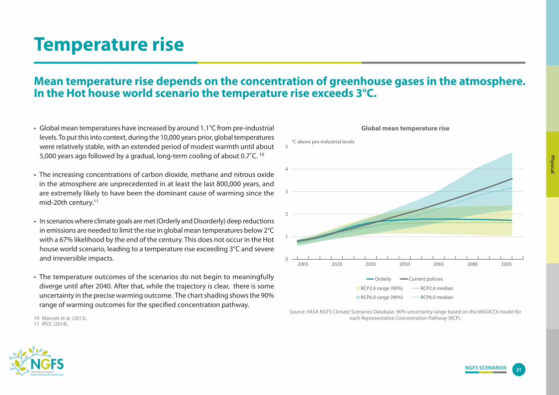
Temperature rise

Mean temperature rise depends on the concentration of greenhouse gases in the atmosphere. In the Hot house world scenario the temperature rise exceeds 3°C.

• Global mean temperatures have increased by around 1.1°C from pre‑industrial levels. To put this into context, during the 10,000 years prior, global temperatures were relatively stable, with an extended period of modest warmth until about 5,000 years ago followed by a gradual, long‑term cooling of about 0.7˚C. 10

• The increasing concentrations of carbon dioxide, methane and nitrous oxide in the atmosphere are unprecedented in at least the last 800,000 years, and are extremely likely to have been the dominant cause of warming since the mid‑20th century.11

• In scenarios where climate goals are met (Orderly and Disorderly) deep reductions in emissions are needed to limit the rise in global mean temperatures below 2°C with a 67% likelihood by the end of the century. This does not occur in the Hot house world scenario, leading to a temperature rise exceeding 3°C and severe and irreversible impacts.

• The temperature outcomes of the scenarios do not begin to meaningfully diverge until after 2040. After that, while the trajectory is clear, there is some uncertainty in the precise warming outcome. The chart shading shows the 90% range of warming outcomes for the specified concentration pathway.

Physical

Source: IIASA NGFS Scenarios Portal. 90% uncertainty range based on the MAGICC6 model for eachRepresentative Concentration Pathway (RCP).

0

1

2

3

4

5

2005 2035 2065 2080 2095

°C above pre-industrial levels

Global mean temperature rise

2020 2050

Current policiesOrderly

RCP2.6 medianRCP2.6 range (90%)

RCP6.0 medianRCP6.0 range (90%)

Source: IIASA NGFS Climate Scenarios Database. 90% uncertainty range based on the MAGICC6 model for each Representative Concentration Pathway (RCP).

Global mean temperature rise

10 Marcott et al. (2013).11 IPCC (2014).

NGFS SCENARIOS 22

Precipitation and flooding

The rise in temperatures leads to increased heavy precipitation across many regions of the world, which in turn increases risks from flooding.

• Global warming will lead to an increase in heavy precipitation and flood risks in most parts of the world.

• Annual maximum discharge (water flow) in a river or watershed is a measure for fluvial flood risk from heavy precipitation.

• In the Hot house world scenario extreme discharge increases sharply in some regions (+27% in North India) and decreases in others (‑30% in Southern Europe). The magnitude of this change increases in warmer climates.

• Losses from acute flood risk will be provided in phase II of the NGFS Climate Scenarios. Wider studies using ISIMIP data suggest that losses would increase by 160%‑240% at 1.5°C of warming (assuming no additional adaptation). At 2°C losses would be twice as high as 1.5°C .12

12 Dottori et al. (2018).

Source: ISIMIP Archive.

Per cent change relative to 1986‑2005

Physical

Changes in annual maximum discharge 3°C of warming in 2100

-30

-20

-10

0

10

20

30Per cent

North India(Ganges)

China(Yangtze/

Yellow)

Source: ISIMIP Archive.

CentralEurope(Rhine)

SouthernEurope

(Spain/Portugal)

Changes in Annual Maximum DischargeCompared to 1986–2005

1.5°C 2.0°C 3.0°C

Source: ISIMIP Archive.

Changes in annual maximum discharge Relative to 1986‑2005

NGFS SCENARIOS 23

Crop yields and food security

Crop yields are complex to model, but evidence suggests that they will be negatively impacted by climate change, particularly in tropical regions.

• Gradual climate change is already impacting crop productivity,13 and this will worsen with higher levels of warming. The adjacent charts show the differences in low production extremes (10y minima) at 1.5°C and 2°C.

• The intensification of low production years is significant across wheat, maize, rice and soy, particularly in tropical regions. These effects are crop‑dependent and more pronounced at higher levels of climate sensitivity (response of temperature to CO2 emissions) due to the potential offsetting fertilisation effects of increased CO2.

• At temperatures higher than 2°C the risks are more substantial. Higher mean temperatures increase the chance that biophysical limits for crop production might be reached. This could have implications for food security and employment, particularly in regions with a relatively large agricultural sector.

13 Moore and Lobell (2015).

Physical

-30

-20

-10

0

10

20

30

1.5°C 2.0°C 1.5°C 2.0°CGlobal Tropical

Source: Schleussner et al. (2018) using data from ISIMIP archive.

Wheat MaizePer cent

-30

-20

-10

0

10

20

30

1.5°C 2.0°C 1.5°C 2.0°CGlobal Tropical

Per cent

Change in crop low production extremes10 year minima in global/tropical production

Source: Schleussner et al. (2018) using data from ISIMIP archive.

Change in crop low production extremes 10 year minima in global/tropical production

NGFS SCENARIOS 24

Other risks

Not all physical risks have been incorporated into the ISIMIP database yet. Some complementary estimates from the wider literature are presented below.14

Heatwaves

• At 3°C+ of warming extreme heatwaves (e.g. Europe in 2003) become more likely. In tropical regions the probability of an extreme heatwave in a given year is projected to be 40%.

Cyclones

• Tropical cyclones are complex to model but emerging evidence suggests that global warming will increase the intensity (1‑10% higher wind speeds) and rain rate (14%) across basins. There is less agreement on the change in frequency.

Sea levels

• Sea levels will continue to rise for centuries to millennia after CO2 emissions have reached net‑zero. 3°C+ of warming implies sea levels rising by almost 2m or more by 2300 (not accounting for low probability high impact scenarios).

Physical

14 Data from the wider literature may be based on different scenario assumptions.

0

50

100

150

200

250

300

350

2100 2300 2100 2300 2100 2300

Long term sea-level riseRelative to 1986-2005

Sea-level rise (cm)

1.5°C 2.0°C

Source: Adapted from Geiges et al. (2019).

3.0°C

Change in tropical cyclone intensity by basin2.0°C of warming

Per cent14

12

10

8

6

4

2

0

-2

-4

-6

-8

-10Global N. Atl. NW Pac. SW Pac.NE Pac.

Source: Knutson et al. (2019).Large whiskers indicate the 10th and 90th percentiles.

N. Ind. S. Ind.

0

10

20

30

40

50Per cent

Extreme heatwave risk

Global Tropics Global Tropics Global Tropics1.5°C 2.0°C

Source: Russo (2020).

3.0°C

Probability of occurrence (%) Exposed population (%)

Source: Adapted from Russo et al. (2015).Source: Adapted from Geiges et al. (2019).

Source: Knutson et al. (2020). Large whiskers indicate the 10th and 90th percentiles.

Extreme heatwave risk Change in tropical cyclone intensity by basin 2°C of warming

Long term sea level rise Relative to 1986‑2005

Scenarios in detail

4 Economic impacts

Economic

NGFS SCENARIOS 26

Approach

The NGFS Climate Scenarios include impacts on GDP from transition risk and physical risk that are modelled separately.

• Modelling the GDP impacts from transition risk and physical risk is subject to significant uncertainty.

• This extends from how emissions will evolve, to the response in climate, to the economic and financial impacts from both. While some of these uncertainties are scenario‑dependent, others relate to the modelling approach employed at each stage.

• There are significant gaps in the literature, which means that the level of uncertainty is likely greater than the ranges shown in this section. For example, studies rarely comprehensively capture tipping points, feedback effects from physical to transition risks, socioeconomic responses such as changing preferences, economic sentiment, migration and adaptation and there are other ‘unknown unknowns’.

• The NGFS will seek to address as many of these gaps as possible in its scenarios through a suite of models approach. This will be an important part of future development.

Economic

Source: James et al. (2017).

Uncertainties in climate change projections

NGFS SCENARIOS 27

Impacts from transition risks

Model estimates of the GDP impact from transition risk display substantial variation, but are typically higher in scenarios with steeper reductions in emissions.

• The figure shows estimates of transition risk impacts from different models and different model calibrations, including from GCAM, MESSAGE and REMIND which are included in the NGFS Climate Scenario database.

• The GDP loss is calculated as relative to the Hot house world scenario (limited mitigation) and does not include impacts from physical risk.

• An important driver of differences in the losses reported by economic models are fundamental model assumptions.

• For example, models that include market frictions and/or agents that make imperfect decisions due to information asymmetries tend to exhibit greater variation in outcomes than models that assume that agents are rational, welfare‑maximising, and have perfect foresight.

Economic

-20

-16

-12

-8

-4

0

Estimates of GDP losses in orderly scenariosBased on IPCC AR5 and the NGFS Orderly scenario (green dot)

2030 2050

Source: Boxplots are based on the IPCC Fifth Assessment Report, Fig. 6.21e.The green dots represent the NGFS Orderly scenario, marker model.

2100

Per cent

Source: Boxplots are based on IPCC (2014), Fig 6.21e. The green dots represent the Orderly scenario, marker model.

Estimates of GDP losses in orderly scenarios Based on IPCC AR5 and the NGFS Orderly scenario (green dot)

NGFS SCENARIOS 28

Uncertainty in impacts from transition risk

Quantifying transition risk is subject to fundamental uncertainty due to model limitations and ‘unknown unknowns’.

• Due to the complex nature and interconnectedness of climate policy, technological progress and consumer preferences, transition risk may materialize in ways that are difficult to foresee.

• Such ‘unknown unknowns’ could, for example, lead to an unexpected technological breakthrough, reducing economy‑wide transition costs, while at the same time creating pressures in certain sectors, with large financial losses as a result.

• Changes in economic sentiment and interactions between the real economy and the financial sector could significantly amplify economic impacts. The 2008 financial crisis demonstrated how these effects can affect growth in the long run (left chart).

• The Integrated Assessment Models used for the NGFS Climate Scenarios do not include these channels in their economic modelling.

Economic

100

110

120

1990 1995

Source: OECD Economic Outlook, Vol. 2018-1.

2000 2005

GDP impact from the 2008 �nancial crisisin OECD countries

180Index (1990 = 100)

170

160

150

140

130

2008

2010 2015

GDP per capita Linear projection

Realeconomy

Financialinstitutions

Financialmarkets

Creditsupply Asset

quality

Interactions between �nance and thereal economy

Monetary and�scal policy

Investorsentiment

Financingconditions

Marketinfrastructure

Source: OECD (2018). Source: Hilbers & Van Hengel (2019).

GDP impact from the 2008 financial crisis in OECD countries

Interactions between finance and the real economy

NGFS SCENARIOS 29

Impacts from physical risks

Global warming, and the associated changes in climate, will have significant impacts on the economy by the end of the century in a Hot house world scenario.

• Estimates of GDP losses from physical risk vary considerably depending on the scenario, assumptions about climate sensitivity and the method used to estimate economic damages.

• The adjacent chart shows GDP impacts from physical risks for the NGFS Climate Scenarios using three damage functions from the literature.

• These estimates underestimate impacts as they do not include all transmission channels and allow for effects on the growth rate. The grey shading represents the uncertainty about climate sensitivity.

• Assessing average losses in this way disguises the significant distribution of impacts across regions. The right chart shows that tropical regions will be disproportionately impacted by heat stress and lower labour productivity. The impacts will vary further depending on regions’ level of resilience and capacity for adaptation.

Economic

DisorderlyOrderly

0

-5

-10

-15

-20

-25

Source: Calculations by PIK based on scenario temperatureoutcomes and damage estimates from the literature.

See NGFS Technical Documentation for further details.

GDP losses in di�erent scenarios usingdi�erent damage functions

2025 2075 2025 2075Hot house world2025 2075

Per cent

Kalkuhl & Wenz (2020), panel, population-weighted

Howard & Sterner (2017)Nordhaus (2017)

Source: Calculations by Climate Analytics based on 3°C of warming, roughly aligned with the NDC scenario.

Source: Calculations by PIK based on scenario temperature outcomes and damage functions from the literature. See Technical

Documentation for further details.

GDP loss from physical risks using different damage functions from the literature

Climate change impacts on labour productivity at 3°C global warming

2100 compared to 1986‑2005

NGFS SCENARIOS 30

Uncertainty in impacts from physical risks

Economic impacts at high degrees of warming would be unprecedented and much more severe than currently estimated given known gaps in modelling.

• There is little agreement across studies about the relationship between temperature and the economy. The adjacent chart shows a range of damage estimates for different levels of warming. The differences arise from the type of modelling approach (e.g. IAM, econometric, CGE), whether impacts are considered to directly affect the growth rate, and the future level of adaptation.

• There are a number of reasons to suggest that these are underestimates of the potential risks. Although some studies capture non‑linearities in biophysical processes as temperatures increase, few fully capture the potential risks of tipping points accelerating global warming. Studies that have assessed the potential impacts from tipping points on policy responses find that emissions prices should be up to eight times higher.

• In addition, the damage estimates shown only cover a limited number of risk transmission channels and tend to ignore the risks from low probability, high impact events (particularly in regions with lower levels of development).

• Another key assumption is that socioeconomic factors such as population, migration and conflict remain constant even at high levels of warming. The World Bank (2018) has suggested that climate change could displace almost 140 million people by 2050 in countries in Sub‑Saharan Africa, Latin America, and Asia.

Economic

Source: As shown. Shade of marker reflects temperature baseline used in the underlying study. Burke, Howard & Sterner (lightest shade) measure temperature rise relative to pre‑industrial levels. Kahn (medium shade) uses a baseline of 1960‑2014. Nordhaus, IMF and Kalkuhl & Wenz (darkest shade) use a

near‑term baseline (ranging from 2005‑present day).

Estimates of GDP losses from rising temperatures in the academic literature

Per cent0

-10

-20

-302.0 2.5 3.0 3.5 4.0 4.5

Nordhaus (2016)

Kahn et al.(2019)

Howard & Sterner (2017)

Burke et al. (2018) Kalkuhl & Wenz (2020)

IMF (2017)

Burke et al. (2018)

Temperature rise (ºC)

5 Future development

Developm

ent

NGFS SCENARIOS 32

Current gaps in scenario modelling

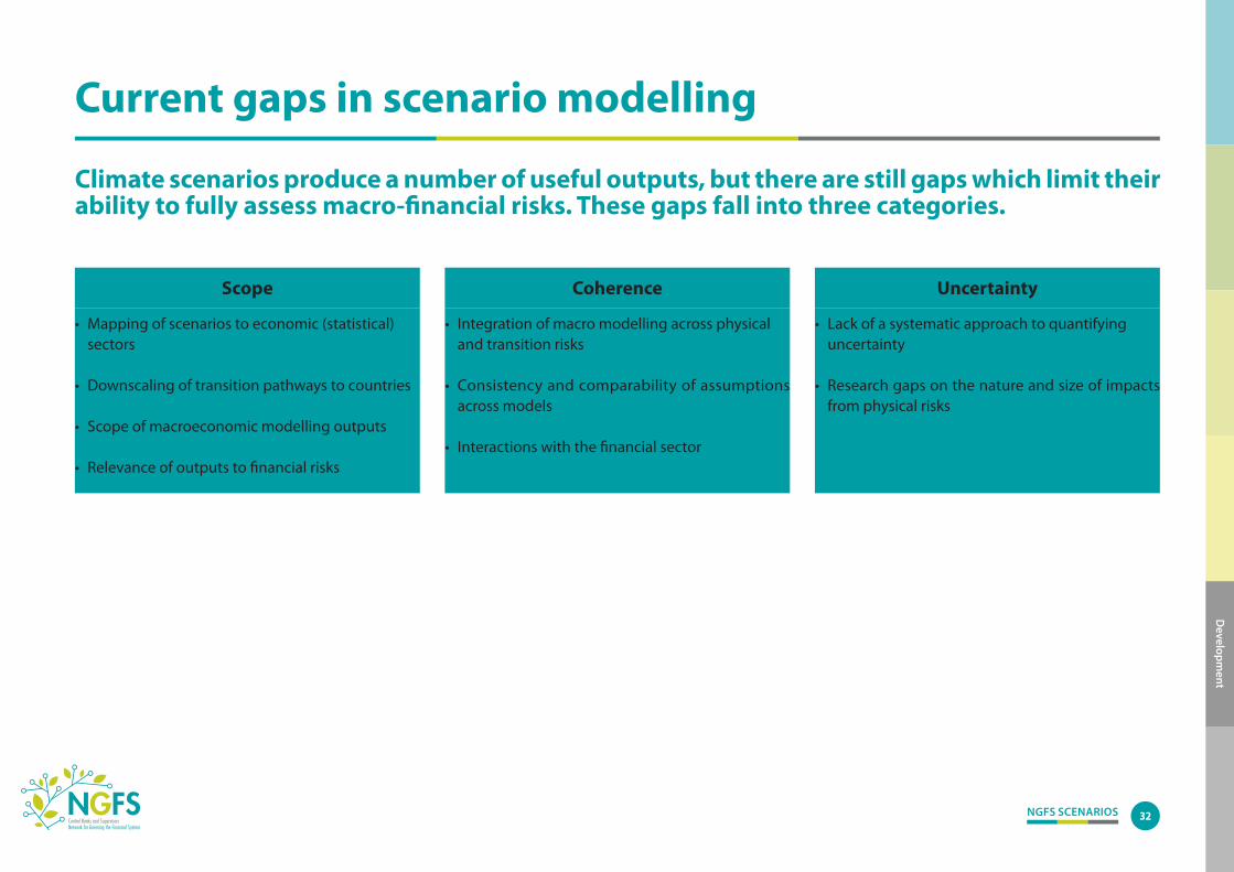
Climate scenarios produce a number of useful outputs, but there are still gaps which limit their ability to fully assess macro-financial risks. These gaps fall into three categories.

• Mapping of scenarios to economic (statistical) sectors

• Downscaling of transition pathways to countries

• Scope of macroeconomic modelling outputs

• Relevance of outputs to financial risks

Scope Coherence Uncertainty

• Integration of macro modelling across physical and transition risks

• Consistency and comparability of assumptions across models

• Interactions with the financial sector

• Lack of a systematic approach to quantifying uncertainty

• Research gaps on the nature and size of impacts from physical risks

Developm

ent

NGFS SCENARIOS 33

Future development

The NGFS will continue to develop the scenarios to make them more comprehensive, with the aim to be as relevant as possible for economic and financial analysis.

Developm

ent

NGFS suite of models approach

Temperaturealignment

Physical riskTransition risk

Macroeconomic impactsGlobal Macroeconomic Models

1.5°C, 2°C, 3°C+

Transitionpathways

Integrated AssessmentModels

Chronic climateimpacts

General CirculationModels

Acute climateimpacts

Natural CatastropheModels

NGFS suite of models approach• Currently there is no single model that can cover the full range of required outputs. In the interim the approach is to use a suite of specialist models linked together in a coherent way.

• Phase I of the NGFS Climate Scenarios delivered a set of harmonised transition pathways, chronic climate impacts and indicative economic impacts for each of the NGFS Climate Scenarios.

• In Phase II the NGFS will continue to work with a consortium of academic partners to refine and expand the scope of the scenarios. Areas of focus will include:

– Expanding the scenario modelling to explore the further dimensions of the risks

– Improving regional coverage and sectoral granularity– Calculating probabilistic losses from acute climate impacts– Expanding the set of macroeconomic outputs– Improving the NGFS Climate Scenario database and portal

NGFS SCENARIOS 34

COVID-19 and the NGFS Climate Scenarios

COVID-19 is having wide ranging impacts on health, the economy, public policy and preferences that will be meaningful for climate scenario analysis.

• COVID‑19 has shown how a system‑wide shock that hits the real economy can have significant effects on economic and financial outcomes. Parallels can be drawn to climate risks where sudden policy or behavioural changes could lead to stranded assets. For the real economy to manage these risks finance will have to play a pivotal role.

• COVID‑19 has already had an immediate impact on GDP, business investment, productivity, unemployment, energy demand and emissions, among other factors.

• The long‑term scale (and in some cases direction) of these effects is unclear. They will depend substantially on the ongoing transmission of the virus and how governments, the general public, companies and the financial sector respond.

• These impacts could affect many of the assumptions that underpin climate models such as population, urbanisation, growth, climate policy, technology and consumer preferences.

–3.0%IMF 2020 Global GDP Projection

–8.0%IEA 2020 Emissions Projection

$2trnSize of the U.S. COVID recovery package alone

+0.8%IEA 2020 Renewable Energy Demand Projection

Developm

ent

References

6 References

NGFS SCENARIOS 36

References

Battiston, S. (2019)The importance of being forward‑looking: managing financial stability in the face of climate risk. Financial Stability Review, Banque de France, 23.

Burke, M., Hsiang, S. M., & Miguel, E. (2015)Global non‑linear effect of temperature on economic production. Nature, 527(7577), 235‑239.

Burke, M., Davis, W. M., & Diffenbaugh, N. S. (2018)Large potential reduction in economic damages under UN mitigation targets. Nature, 557(7706), 549‑553.

Cochrane, E. & Fandos, N. (2020, May 5)Senate Approves $2 Trillion Stimulus After Bipartisan Deal. The New York Times. Retreived from https://www.nytimes.com/2020/03/25/us/politics/coronavirus-senate-deal.html.

Dottori, F., Szewczyk, W., Ciscar, J. C., Zhao, F., Alfieri, L., Hirabayashi, Y., … & Feyen, L. (2018)Increased human and economic losses from river flooding with anthropogenic warming. Nature Climate Change, 8(9), 781‑786.

Frieler, K., Lange, S., Piontek, F., Reyer, C. P., Schewe, J., Warszawski, L., ... & Geiger, T. (2017)Assessing the impacts of 1.5°C global warming–simulation protocol of the Inter‑Sectoral Impact Model Intercomparison Project (ISIMIP2b). Geoscientific Model Development.

Geiges, A., Parra, P. Y., Andrijevic, M., Hare, W., Nauels, A., Pfleiderer, P., Schaeffer, M. & Schleussner, C.-F. (2019)Incremental improvements of 2030 targets insufficient to achieve the Paris Agreement goals, Earth Syst. Dynam. Discuss.

Hilbers, P., & Van Hengel, M. (2019)Putting macroprudential policy to work: a case study on the Dutch housing market. SUERF Policy Note, Issue No 115.

Howard, P. H., & Sterner, T. (2017)Few and not so far between: a meta‑analysis of climate damage estimates. Environmental and Resource Economics, 68(1), 197‑225.

IEA (2020)Global Energy Review 2020, IEA, Paris https://www.iea.org/reports/global-energy-review-2020.

IIASA, NGFS Climate Scenarios Database (2020)Available at https://data.ene.iiasa.ac.at/ngfs/.

IMF (2020)World Economic Outlook, April 2020: “The Great Lockdown”. International Monetary Fund, Washington, DC. https://www.imf.org/en/Publications/WEO/Issues/2020/04/14/weo-april-2020.

References

NGFS SCENARIOS 37

IPCC (2014)Climate Change 2014: Synthesis Report. Contribution of Working Groups I, II and III to the Fifth Assessment Report of the Intergovernmental Panel on Climate Change [Core Writing Team, R.K. Pachauri and L.A. Meyer (eds.)]. IPCC, Geneva, Switzerland, 151 pp.

IPCC (2014)AR5 Scenario Database. Available at https://tntcat.iiasa.ac.at/AR5DB/.

IPCC (2018)Global Warming of 1.5°C, an IPCC special report on the impacts of global warming of 1.5°C above pre-industrial levels and related global greenhouse gas emission pathways, in the context of strengthening the global response to the threat of climate change, sustainable development, and efforts to eradicate poverty. [Masson‑Delmotte, V., P. Zhai, H.‑O. Pörtner, D. Roberts, J. Skea, P.R. Shukla, A. Pirani, W. Moufouma‑Okia, C. Péan, R. Pidcock, S. Connors, J.B.R. Matthews, Y. Chen, X. Zhou, M.I. Gomis, E. Lonnoy, T. Maycock, M. Tignor, and T. Waterfield (eds.)]. In Press.

James, R., Washington, R., Schleussner, C. F., Rogelj, J., & Conway, D. (2017)Characterizing half‐a‐degree difference: a review of methods for identifying regional climate responses to global warming targets. Wiley Interdisciplinary Reviews: Climate Change, 8(2), e457.

Kahn, M. E., Mohaddes, K., Ng, R. N., Pesaran, M. H., Raissi, M., & Yang, J. C. (2019)Long-term macroeconomic effects of climate change: A cross-country analysis (No. w26167). National Bureau of Economic Research.

References

Kalkuhl, M., & Wenz, L. (2020)The Impact of Climate Conditions on Economic Production. Evidence from a Global Panel of Regions. Working paper, ZBW – Leibniz Information Centre for Economics, Kiel, Hamburg.

Knutson, T., Camargo, S. J., Chan, J. C., Emanuel, K., Ho, C. H., Kossin, J., ... & Wu, L. (2020)Tropical cyclones and climate change assessment: Part II: Projected response to anthropogenic warming. Bulletin of the American Meteorological Society, 101(3), E303‑E322.

Marcott, S. A., Shakun, J. D., Clark, P. U., & Mix, A. C. (2013)A reconstruction of regional and global temperature for the past 11,300 years. Science, 339(6124), 1198‑1201.

McCollum, D. L., Zhou, W., Bertram, C., De Boer, H. S., Bosetti, V., Busch, S., ... & Fricko, O. (2018)Energy investment needs for fulfilling the Paris Agreement and achieving the Sustainable Development Goals. Nature Energy, 3(7), 589‑599.

Mejia, M. S. A., Mrkaic, M. M., Novta, N., Pugacheva, E., & Topalova, P. (2018)The Effects of Weather Shocks on Economic Activity: What are the Channels of Impact?. International Monetary Fund, Washington, DC.

Moore, F. C., & Lobell, D. B. (2015)The fingerprint of climate trends on European crop yields. Proceedings of the National Academy of sciences, 112(9), 2670‑2675.

References

NGFS SCENARIOS 38

References

NGFS (2019a)A call for action: Climate change as a source of financial risk. First Comprehensive report, Network for Greening the Financial System, Paris, France 42 pp.

NGFS (2019b)Macroeconomic and financial stability: Implications of climate change. Technical supplement to the First NGFS Comprehensive Report, Network for Greening the Financial System, Paris, France, 51 pp.

NGFS (2020)Technical documentation to the NGFS Climate Scenarios. Network for Greening the Financial System, Paris, France, 66 pp.

Nordhaus, W. D. (2016)Projections and Uncertainties About Climate Change in an Era of Minimal Climate Policies. NBER Working Paper, (w22933).

Nordhaus, W. D. (2017)Revisiting the social cost of carbon. Proceedings of the National Academy of Sciences, 114(7), 1518‑1523.

OECD (2018)OECD Economic Outlook, Volume 2018 Issue 1. OECD Edition, Paris.

Riahi, K., Van Vuuren, D. P., Kriegler, E., Edmonds, J., O’Neill, B. C., Fujimori, S., ... & Lutz, W. (2017)The shared socioeconomic pathways and their energy, land use, and greenhouse gas emissions implications: an overview. Global Environmental Change, 42, 153‑168.

Russo, S., Sillmann, J. & Fischer, E.M. (2015)Top ten European heatwaves since 1950 and their occurence in the coming decades. Environmental Research Letters, 10(12).

Schleussner, C. F., Deryng, D., Müller, C., Elliott, J., Saeed, F., Folberth, C., ... & Seneviratne, S. I. (2018)Crop productivity changes in 1.5°C and 2°C worlds under climate sensitivity uncertainty. Environmental Research Letters, 13(6), 064007.

UNEP (2018a)Emissions Gap Report. UNEP, Nairobi.

UNEP (2018b)Extending our horizons: Assessing Credit Risk and Opportunity in a Changing Climate. UNEP, Nairobi.

World Bank (2018)Groundswell – Preparing for Internal Climate Migration. The World Bank, Washington, DC.

References

NGFSSecretariat