nexus express quick reference card
TRANSCRIPT

NexusExpressQuickReferenceCard
1. Open an existing project or create a new project from the start page or the File menu.
2. When creating a new project, Click the Load Load Data button to add data to the project.
In the “Copy number” tab, select “Affymetrix‐OSCHP ‐ TuScan” as the data type for OncoScanTM FFPE Assay Kit copy
number data. If you would like to also view Somatic Mutations within your OncoScanTM data, please select the top check
box “Also load associated Seq View data”. If you would like to have the data process immediately after loading your
OSCHP files, check the box “Automatically Start Processing After Data Loading”. Click on the “Select Files” button and an
explorer window will appear. Navigate to your OSCHP files, select the files you would like to view and click “Done”.

3. Review your analysis parameters
In the Dataset Tab, if you did not select the option “Automatically Start Processing” above, please click the
“View” button to process your OSCHP files. Click on “Processed” in the “Status” column for a given sample to
have the “Settings” dialog box appear. Under “Analysis” you can see the algorithm used to process the data.
Affymetrix’s TuScan algorithm is the recommended default algorithm for OncoScanTM data. The alternative
algorithm is SNPFASST2 from BioDiscovery. If analyzing the OncoScanTM data with SNPFASST2, please go to page
14 of this QRC.


4. In the Dataset tab, you can review the TuScan algorithm metrics for OS‐MAPD,OS‐ ndSNPQC, OS‐
ndWavinessSd, OS‐CellCheckPairStatus, OS‐% Aberrant Cell, OS‐Ploidy, and OS‐ Low Diploid Flag. For
details descriptions of these metrics, please refer to the OncoScan Console Software User Manual.
5. Once all samples are in a “processed” status, the samples will be displayed in the Results Tab which is a
multi‐sample view. All the samples in the project (or the ones for which you have selected the check
box in the Dataset Tab), will be listed on the left of the Results tab. The top graph allows for viewing
common aberrations across the dataset. In the example below, ~50% of the samples have a gain on
Chromosome 5 (black circle). To drill down into a specific sample, click on the name of the sample on
the left of the screen (arrow).
Single Sample Data Analysis/Interpretation:
1. From the Results Tab. click on the OSCHP file name to bring up the individual sample details.
2. First, determine if the sample needs re‐centering (adjustment for ploidy).
a. In the “Sample Info”, check if “OS Diploid Flag” is “Yes”. This usually indicates Ploidy correction is
needed.
b. Click the “Overview” tab (arrow) in the sample drill down window.

c. If there are regions of allelic imbalance (indicated by purple shading of the chromosome) that do not
have copy number changes associated with them (blue or red bars next to the chromosome) probe
centering is likely required. Also, if there are regions of loss (indicated by a red bar to the left of the
chromosome) that have no allelic imbalance or LOH, probe centering is likely needed.
See the example below:

IMPORTANT: The following section on recentering the sample in the software is applicable for the
SNPFASST2 algorithm only.
d. Click on the “Whole Genome” tab (arrow in figure below) in the sample drill down to display the
intensity and B‐allele frequency information across the whole genome. [ NOTE: Another check to see if
the sample needs recentered is to examine the autosomal regions with 3 tracks in the BAF graph that
are being called as a loss or a gain according to the logR graph. This would also indicate the sample likes
needs corrected in terms of ploidy.]. In the sample below, we have already seen that the Overview
suggest this sample might need recentered. In looking at the Whole Genome View, the logR graph for
Chromosome 3p and 14 indicates a loss, whereas the BAF track has 3 tracks representing at least 2
alleles and therefore indicating this sample needs recentering. [For some samples, one may need to
identify regions that have 3 tight bands on the BAF, but in the logR graph are elevated above the 0
(diploid) line.]
e. Examine the intensity and B‐allele frequency data to identify diploid regions. Zoom into the diploid
region using the rectangular zoom tool .
f. Click the “Set Diploid Regions” button ( ) and then click the “Add Region” button. Add as many
diploid regions as necessary and then click “Apply” to initiate reprocessing of the sample setting the
identified regions to CN=2.
The figure below shows the same sample after recentering using Chromosome 14 as baseline. Those regions
with 3 tracks in the BAF now have a logR graph centered at 0 which is a more likely scenario. [Note that in
the cases where the ploidy is 4, there may be 3 allele tracks as each chromosome may have duplicate
resulting in no allelic imbalance.]

3. Use the Whole Genome View to identify gains, losses, LOH and copy neutral LOH, by reviewing the log2 and the BAF
tracks together. In the example below, Chromosome 4 shows diploid on the p arm (logR at 0 and 3 BAF tracks), while
the q arm shows a loss (downward shift of the logR data and 4 BAF tracks, red oval). Chromosome 13 is an example
of a gain (upward shift of the logR data and 4 BAF tracks, black oval). The interstitial region of Chromosome 7 shows
copy neutral LOH (logR data at 0 and 4 BAF tracks, arrow).

4. Use the Chromosome view to zoom to probe level, and to view copy number aberrations. To view copy number in a
gene of interest, type “the gene name” in the search box and click Find. The software will zoom into that gene. You
can mouse over the aberration to get linear copy number call. For example, screen shot of an aberration with a
linear copy number of 5.0 for the MDM2 gene is shown below.
5. To view the Somatic Mutation data for each sample, click on the Seq Variants tab located under the graphs on the
Chromosome tab (red arrow) . This table lists somatic mutation annotation information as well as provides a call for
each mutation in the assay in the MutCal column. In the figure below, the oval outlines a somatic mutation with a
high confidence call for that particular mutation.

6. To view samples that contain aberrations in a list of genes, go to the “Dataset” tab, click on the Query button
(located in the red circle in the image below). Type your list of genes or load a tab delimited text file with the gene
names, click Run. You can quickly identify the samples in the project that have aberrations in your genes of interest.

7. You can compare copy number data between groups, (e.g., Tumor and Normal) using the comparison analysis
functionality.
a. In the “Dataset” tab, sample information can be added to the project either by clicking the Factors drop
down button and then selecting either Add Factor to enter the data manually or “Load Factor” to read

data from a tab‐delimited text file. Below we are manually adding a “Prognosis” factor. Click OK to add
a Prognosis Factor column to the dataset.
b. If you are not importing factors from a tab‐delimited file, manually enter each Factor field by clicking in
the text box for the appropriate samples. The figure below shows the Prognosis for each sample as
Good, Intermediate, Poor in the far right column.
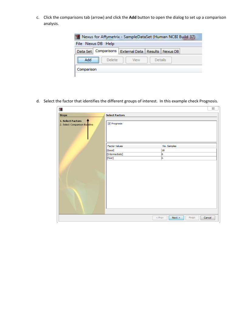
c. Click the comparisons tab (arrow) and click the Add button to open the dialog to set up a comparison
analysis.
d. Select the factor that identifies the different groups of interest. In this example check Prognosis.

e. Select the baseline to be used in the analysis. In this example, select “Sequential “which will analyze
each group against the other 2 groups individually. Click Finish.
f. Highlight the comparison you would like to view (e.g., Poor vs. Good). The View button should now be
enabled, click View to see the results.

8. Use the “Regions”, “Genome”, and “Chromosome” tabs to explore the copy number changes between selected
groups. Below illustrates a region on Chromosome 22 covering the GSTTP1 gene in which the patients with Poor
Prognosis show a loss and the patients with Good Prognosis have no aberration.
Analysis of OncoScanTM Assay Data using SNPFASST2
Affymetrix recommends analyzing OncoScanTM Assay data using our TuScan algorithm. The Nexus Express software
does enable you to analyze the data using the BioDiscovery SNPFASST2 algorithm as well. If you would like to view
your data using SNPFASST2, please follow the following steps. To enabling comparison of the different segmentation
algorithms in the same project, please make a copy of the OSCHP file on your computer.
1. Duplicate your data on your computer.
a. Example: Make a copy of RenalCancer.OSCHP and append an “_1”
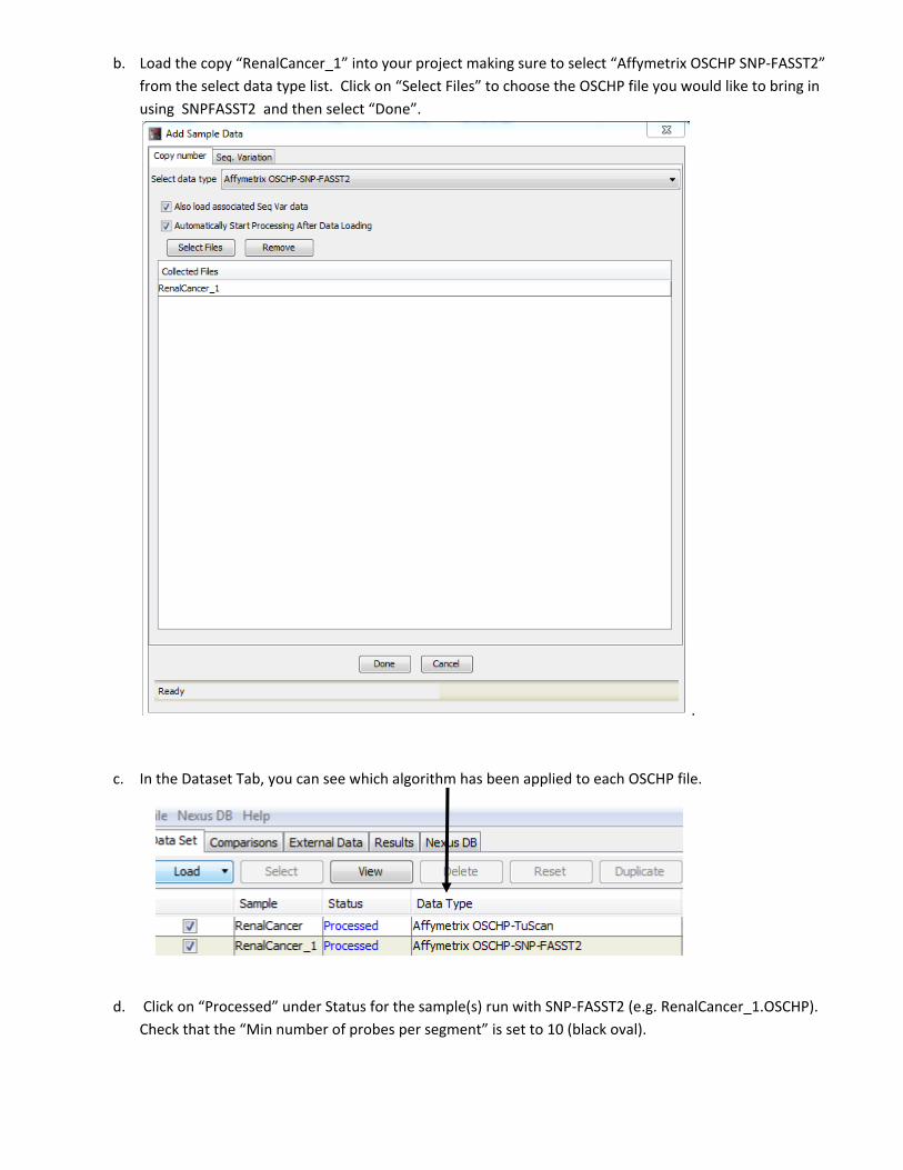
b. Load the copy “RenalCancer_1” into your project making sure to select “Affymetrix OSCHP SNP‐FASST2”
from the select data type list. Click on “Select Files” to choose the OSCHP file you would like to bring in
using SNPFASST2 and then select “Done”.
.
c. In the Dataset Tab, you can see which algorithm has been applied to each OSCHP file.
d. Click on “Processed” under Status for the sample(s) run with SNP‐FASST2 (e.g. RenalCancer_1.OSCHP).
Check that the “Min number of probes per segment” is set to 10 (black oval).

e. If you would like to change the “Min number of probes per segment” from the recommended 10, please
go back to the Dataset Tab. Highlight the sample file that was run with SNPFASST2 and click on “Duplicate”.

f. Uncheck all boxes except for those OSCHP files you would like to process using a different “Min number of
probes per segment”. Go to File Settings , make sure the data type is on “Affymetrix OSCHP SNP‐
FASST2” and then you can alter the “Min number of probes per segment” value (e.g. 20). Click the “Done”
button.
g. Click on “View” to process the data.
h. Please return to Step C on page for to follow the workflow. Please keep in mind that linear copy number is
not available for the SNPFASST2 algorithm.