newsletter en38 v1 - mercator ocean faucher et al. provide a description of a coupled...

Mercator Ocean Quarterly Newsletter #38 – July 2010 –

GIP Mercator Ocean

Quarterly Newsletter

Strandings of green macroalgae on beaches and coves along the Brittany coast. (See paper by

Ménesguen et al. in the present issue). Credits: media.paperblog.fr

Editorial – July 2010 Greetings all,

This month’s newsletter is devoted to recent studies in coastal oceanic systems.

To start with, Le Traon is introducing this newsletter telling us about the SNOCO initiative.

Scientific articles about recent studies in coastal oceanic systems are then displayed as follows: First, Ménesguen et al. are telling

us about Ulva mass accumulations on Brittany beaches and remedies found to solve this problem. Then, Ardhuin presents his

work about wave hindcasting and forecasting at Previmer within the European project “Integrated Ocean waves for Geophysical

and other Applications”. Third, Faucher et al. provide a description of a coupled Atmosphere-Ocean-Ice forecast system for the

Gulf of St Lawrence in Canada, which has been installed in experimental mode at the Canadian Meteorological Centre. Finally,

Marchesiello et al. are talking about regional ocean forecasting and downscaling strategy at IRD for coastal and submesoscale

phenomena. They have developed a downscaling strategy based on the Regional Ocean Modeling System and produced a new

demonstrator with data assimilation in the Chile oceanic area.

The next October 2010 newsletter will display papers about the Marginal Seas in the MyOcean project.

We wish you a pleasant summer!


GIP Mercator Ocean

Contents

SNOCO: Towards a French Sustained Coastal Operational Oceanography System ..........................................3

By Pierre Yves Le Traon

Ulva Mass Accumulations on Brittany Beaches: Explanation and Remedies Deduced from Models................4

By Alain Ménesguen, Thierry Perrot, Morgan Dussauze

Wave Hindcasting and Forecasting: Geophysical and Engineering Applications. Examples with the Previmer-

IOWAGA System. ..........................................................................................................................................14

By Fabrice Ardhuin

Coupled Atmosphere-Ocean-Ice Forecast System for the Gulf of St-Lawrence, Canada ................................23

By Manon Faucher, François Roy, Hal Ritchie, Serge Desjardins, Chris Fogarty, Greg Smith, Pierre Pellerin

Regional Ocean Forecasting : Downscaling Strategy for Coastal and Submesoscale Phenomena ..................32

By Patrick Marchesiello, Zhijin Li and Andres Sepulveda

Notebook ......................................................................................................................................................38


SNOCO : Towards a French Sustained Coastal Operatio nal Oceanography System

SNOCO: Towards a French Sustained Coastal Operation al Oceanography System By Pierre-Yves Le Traon 1 1IFREMER/BREST, Plouzané, France

Over the past decade, there have been major improvements in the development of global operational oceanography. France set

up in 1997 its contribution to the international GODAE experiment for the three main components: satellite observations (Jason

series), in situ observations (with Coriolis including the French contribution to Argo) and modeling and data assimilation with

Mercator Ocean. These efforts have strongly contributed to the development of the European GMES Marine Core Service. In

2005, a French inter-agency cooperation started to develop plans for the establishment of a national coastal operational

oceanography system. Demonstrators on the three coastal metropolitan facades were put in place, in particular, in the context of

the PREVIMER project (see www.previmer.org). These demonstrators have shown the capacity to provide observations and

forecasts of French coastal areas.

Mercator Ocean has demonstrated its capacity to provide global and regional ocean services at national and European level with

MyOcean and the GMES Marine Core Service. Thanks to the PREVIMER demonstration, there is now a capacity of moving

towards an integrated open sea and coastal operational oceanography service ensuring a wider geographical coverage and level

of service tailored to the coastal areas. This service should cover the three Metropolitan facades (Channel, Atlantic,

Mediterranean) with a gradual extension of French overseas coastal areas. Extending current capabilities at the coast where

societal needs, economic and public policy requirements are the strongest is both necessary and strategic for France.

Such a proposal was made at the last Conseil Interministériel de la Mer (CIMER) in December 2009 who decided that France

should gradually establish a public service for coastal operational oceanography, based on an in-situ observing infrastructure and

an analysis and forecasting system. The so called SNOCO (Service National d’Océanographie Côtière) should be coupled to

Mercator Ocean and the GMES Marine Core Service to provide a seamless description of the ocean state from the open ocean

down to the coastal zone. It should meet the needs of maritime policy and coastal environment monitoring (e.g. marine strategy),

marine renewable energy, aquaculture and fishery management, health, public safety and security, defense, research...

The different participating agencies are now analyzing how they can contribute to the SNOCO. The objective is to find an

agreement by the end of 2010 and to develop a project to make sure that after the end of PREVIMER (2012) a sustained service

and organization is put in place. This new ocean analysis and forecasting capability will be naturally strongly linked to Mercator

Ocean.

Mercator Ocean Quarterly Newsletter #38 – October 2010 –

Ulva Mass Accumulations on Brittany Beaches: Explan ation and Remedies Deduced from Models

Ulva Mass Accumulations on Brittany Beaches: Explan ation and Remedies Deduced from Models By Alain Ménesguen 1 , Thierry Perrot 2, Morgan Dussauze 1 1 IFREMER/BREST, Département DYNECO, Plouzané, France 2CEVA, Pleubian, France

Abstract

During the seventies, a growing number of beaches and coves along the Brittany coast (western France) have been invaded

every year, from spring to autumn, by huge strandings of green macroalgae (free-floating ulvae). This typical eutrophication

phenomenon has now reached a quasi-steady state, with high biomasses during « wet » years, and lower biomasses during

« dry » ones. Studies focused on the Saint-Brieuc and Lannion bays explained this proliferation and accumulation of green algae

by the conjunction of a natural confinement of some shallow water masses, despite the strong tidal movement, with a recent, man-

made nitrate enrichment of these coastal marine waters. In these confined embayments, algal biomass observed at the beginning

of summer correlates very well with the late spring nitrate loadings brought by the tributaries; the summer decline of these

loadings induces the drop in the nitrogen internal quota of ulvae, which stops the algal growth in summer. The mathematical 3D

model of these « green tides », developed by Ifremer and currently exploited by CEVA, shows in every bay that the only way to

decrease the ulva biomass is to dramatically lower the nitrate terrestrial loadings from agricultural origin. A new numerical

tracking technique applied to the nitrogen in the whole ecosystem model has quantified the actual role of each tributary in the

algal nitrogen fueling. Above the most sensitive embayments, the nitrate concentration in the tributaries should be reduced from

the actual 30-40 mg/L to 5-10 mg/L, which constitutes a tremendous challenge for the intensive agriculture. One century ago,

nitrate concentration in Brittany rivers was probably around 1-3 mg/L…

Introduction

Green marine macroalgae (Ulva, Enteromorpha, Monostroma,…) have been known for a while as indicators of strong nitrogen

enrichment of the marine waters: they proliferate in coastal, very shallow areas which receive heavy loadings of inorganic

nitrogen, mainly of land runoff origin (nitrate), but sometimes of urban sewage origin (ammonia or nitrate). Ulva mass blooms have

been frequently reported during spring and summer in coastal, semi-enclosed lagoons (Venice, Tunis, Mediterranean coast of

France), but a new, rather paradoxical, type of mass accumulations of Ulva did appear 40 years ago in Brittany(France), along

beaches largely open to the sea and subject to a strong tidal movement twice a day. In the first half of the 20th century, nobody

had forecasted the possible appearance of such proliferations and accumulations in such open tidal embayments. Year after year,

the regular come back of this huge pollution in touristic spots has induced a substantial financial loss, as well as a growing anger

of local populations, which recently culminated in July 2009: the death, in a few minutes, of a horse stuck in rotting green algae on

a beach proved that the hydrogen sulphide produced by the anaerobic decomposition of algae could be extremely dangerous for

humans and animals. A study of this so-called “green tides” phenomenon was undertaken by IFREMER and CEVA at the end of

the eighties. This paper will recall the main explanations found 20 years ago, then present the modelling tools specially designed

during the last decade for testing remediation scenarios, and finally give the main results and recommendations which came out of

this long modelling effort.

Overview of the phenomenon

Annual inquiries into the volumes of algae collected by the coastal city councils have been made by CEVA since 1978. They

reveal a globally stable location of the main spots of significant algal deposits along the Brittany coast, which has been

corroborated by regular photographical aerial surveys made during the last twenty years (Figure 1). The total biomass present in

July along Brittany can be estimated between 50 000 and 100 000 tons of wet weight; the most polluted sites are large sandy

beaches along the northern and western coast of Brittany (Saint-Brieuc, Saint-Michel-en-grève, Sainte-Anne-la-Palud), whereas

silty very shallow embayments and estuarine shores are more numerous along the western (Brest) and the southern coasts of

Brittany (La Forêt-Fouesnant). The species involved are Ulva armoricana (mainly in the north) et Ulva rotundata (mainly in the

south). The local biomass starts in April by very small fragments of ulva thallus, which are free-floating in the surf zone of the

beaches or near the bottom of shallow coves. It increases dramatically in June, and can cover in July a great part of the beaches,

especially at ebb during calm weather (Figure 2). Algae that have been deposited in the upper part of beaches by high tide flood

will stay there during a fortnight, drying at the top of the deposit and decaying in anaerobic conditions under this superficial,

impermeable crust. In these rotting algal deposits, hydrogen sulphide gas can accumulate up to very high concentrations (> 1000

ppm), and then produce lethal outbursts when humans or animals walk into these deposits.



Figure 1 - Map of “green tides” observed in summer 2008 (disk surface is related to the total area covered by ulvae observed at

three moments: May, July and September). (source: CEVA)

The inaccessibility of beaches to traditional seaside touristic use, as well as the real sanitary risk, compels coastal cities to

implement an expensive regular collecting of stranded algae by bulldozers and trucks. This does not really clean the beach, and

can pick up too much sand, but amounts every year to about half a million euros, and certainly two or three times more if an

exhaustive collecting is now planned to avoid sanitary risks. The collected biomass was partially used as a fertilizer in agriculture

until 2009, but without any corresponding decrease in chemical fertilizers: this contributed to maintain a vicious circle of unlimited

enrichment of coastal water masses.

Figure 2 - Complete coverage of Saint-Michel-en-grève beach by stranded ulvae at ebb in summer (© CEVA)



The appearance of the « green tides » in Brittany can be roughly established around the end of the sixties. Even if some small

deposits could regularly occur in some enclosed parts of the coasts, aerial photographs taken during the second half of the 20th

century clearly show the settlement of the phenomenon: for example, the bay of Guisseny (northern Brittany), which is now a « hot

spot », was totally free from ulva deposits in 1952 and 1961, began to be invaded in 1978, and has been heavily polluted from

1980 until now. The most famous « green tide » in Brittany, which is to be found on the Saint-Michel-en-grève beach, led the local

inhabitants to sign their first protest against unacceptable alteration of their beach in 1971. So, the number of eutrophicated

embayments, as well as the total ulva biomass they produce in a year, dramatically increased during the seventies, and reach a

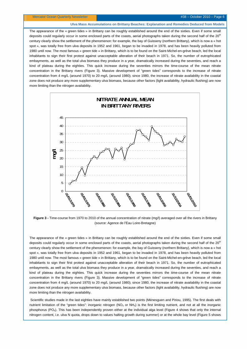
kind of plateau during the eighties. This quick increase during the seventies mirrors the time-course of the mean nitrate

concentration in the Brittany rivers (Figure 3). Massive development of “green tides” corresponds to the increase of nitrate

concentration from 4 mg/L (around 1970) to 20 mg/L (around 1980); since 1980, the increase of nitrate availability in the coastal

zone does not produce any more supplementary ulva biomass, because other factors (light availability, hydraulic flushing) are now

more limiting than the nitrogen availability.

NITRATE ANNUAL MEAN IN BRITTANY RIVERS

0

5

10

15

20

25

30

35

40

45

01/01/1970

01/01/1975

01/01/1980

31/12/1984

01/01/1990

01/01/1995

01/01/2000

31/12/2004

01/01/2010m

g/L

Figure 3 - Time-course from 1970 to 2010 of the annual concentration of nitrate (mg/l) averaged over all the rivers in Brittany

(source: Agence de l’Eau Loire-Bretagne)

The appearance of the « green tides » in Brittany can be roughly established around the end of the sixties. Even if some small

deposits could regularly occur in some enclosed parts of the coasts, aerial photographs taken during the second half of the 20th

century clearly show the settlement of the phenomenon: for example, the bay of Guisseny (northern Brittany), which is now a « hot

spot », was totally free from ulva deposits in 1952 and 1961, began to be invaded in 1978, and has been heavily polluted from

1980 until now. The most famous « green tide » in Brittany, which is to be found on the Saint-Michel-en-grève beach, led the local

inhabitants to sign their first protest against unacceptable alteration of their beach in 1971. So, the number of eutrophicated

embayments, as well as the total ulva biomass they produce in a year, dramatically increased during the seventies, and reach a

kind of plateau during the eighties. This quick increase during the seventies mirrors the time-course of the mean nitrate

concentration in the Brittany rivers (Figure 3). Massive development of “green tides” corresponds to the increase of nitrate

concentration from 4 mg/L (around 1970) to 20 mg/L (around 1980); since 1980, the increase of nitrate availability in the coastal

zone does not produce any more supplementary ulva biomass, because other factors (light availability, hydraulic flushing) are now

more limiting than the nitrogen availability.

Scientific studies made in the last eighties have mainly established two points (Ménesguen and Piriou, 1995). The first deals with

nutrient limitation of the “green tides”: inorganic nitrogen (NO3 or NH4) is the first limiting nutrient, and not at all the inorganic

phosphorus (PO4). This has been independently proven either at the individual alga level (Figure 4 shows that only the internal

nitrogen content, i.e. ulva N quota, drops down to values halting growth during summer) or at the whole bay level (Figure 5 shows



that the summer peak of stranded biomass is linearly correlated with June nitrate loadings, but not at all with phosphate ones).

The second point concerns the accumulation capability of some tidal embayments: hydrodynamical models have allowed to

compute the tidal residual circulation and to show that some areas near the coast can exhibit very low residual drift of the water

mass, favouring long residence time of river-born nutrients in shallow water bodies. For instance, this mechanism transforms the

southern coastal fringe of the bay of Saint-Brieuc (Figure 6) into a wide and shallow retention area, associated to the largest

“green tide” in Brittany.

Figure 4 - Seasonal evolution from April to November of the nitrogen and phosphorus contents (% of dry weight) of individual

ulvae taken in the “green tide” of the Saint-Brieuc bay (source: CEVA).

Figure 5 - Empirical relationships between maximum annual peak of ulva biomass (tons of wet weight) in the southern bay of

Saint-Brieuc and loadings from tributaries in June (Ménesguen and Piriou, 1995) 1) of nitrate (left panel) in kg of N per day; 2) of

phosphate (right panel) in kg of P per day.



Figure 6 - Map of residual tidal currents (m/s) and Ulva strandings in the southern bay of Saint-Brieuc (Ménesguen and Salomon,

1988).

Description of the modelling tools

The Ulva model has been developed at the end of the eighties by Ifremer, as a module of a more general biogeochemical model

of the Nitrogen, Phosphorus and Silicon cycling in the coastal ocean.

The hydrodynamical context of this ecosystem model has been successively furnished by simple box-models of residual

circulation (Ménesguen et Salomon, 1988), 3D finite difference model with non-uniform rectangular horizontal computational grid

and Z vertical coordinates (SiAM3D model, Cugier and Le Hir 2002), and 3D finite difference model with uniform square grid and

σ vertical coordinates (MARS3D model, Lazure and Dumas, 2008). The 3D models have allowed to use refined grids in areas of

interest, typically with a 150m horizontal mesh size for an eutrophicated cove along the Elorn estuary in the bay of Brest

(Ménesguen et al., 2006), or the whole southern area of the bay of Saint-Brieuc (Perrot et al., 2007). These 3D models provide

water surface elevation and velocities in the three space directions at each node of the grid, and solves an advection-dispersion

equation for temperature, salinity, inorganic suspended matter and, more generally, any dissolved and/or particulate variable. The

models are forced with tidal harmonic components at the marine boundaries, with measured flows and concentrations at river

boundaries and with wind-induced stresses at the surface. Flow rates and nutrient concentrations in the tributaries are provided by

the French national databases (http://www.hydro.eaufrance.fr and http://www.surveillance.eaufrance.fr/parametres). Heat and

movement transfer at the ocean-surface interface is calculated using computed fields of meteorological variables from Meteo-

France ARPEGE model (air temperature, cloud cover, relative humidity, wind and atmospherical pressure.



Figure 7 - Schematic flow chart of the biogeochemical model including suspended and settled ulvae (Ménesguen et al., 2006).

In order to be able to take into account the competition between phytoplankton and macroalgae in shallow eutrophicated zones,

the biological sub-model describes nitrogen, silicon and phosphorus cycles. An overview of the structure of the whole

biogeochemical model is reminded in Figure 7. The state variables of the basic model are those currently used in the so-called

“NPZD models”, i.e. dissolved inorganic nutrients [here, NH4, NO3, PO4, Si(OH)4], phytoplankton (here diatoms, dinoflagellates

and nanoflagellates), zooplankton (microzooplankton and mesozooplankton), detrital forms (here, particulate detrital N, particulate

detrital P and biogenic particulate Si). In competition with the three phytoplanktonic forms, a Ulva module is added, containing 6

new state variables: biomass of 1) suspended and 2) settled forms of Ulva, nitrogen mass of 3) suspended and 4) settled forms

of Ulva and phosphorus mass of 5) suspended and 6) settled forms of Ulva.

In a classical fashion, Ulva growth rate is the product of a potential growth rate modulated by temperature and the minimum

between respective light and nutrient limiting effects; temperature effect is considered as obeying a classical "Q10=2" law (Raven

and Geider, 1988) in the range 0-25°C. Similarly to phytoplanktonic variables, the Ulva photosynthesis-light curve is assumed to

obey a saturation Smith’s function without photo-inhibition at high enlightment (Smith, 1936). For suspended ulvae, the light effect

function is then integrated between the ceiling and the floor of the water layer. For settled ulvae, the light effect function is

calculated using directly the light available at the sea bottom, but applies only for the superficial part of the deposit, which cannot

be greater than a fixed threshold (the excess of settled biomass is considered as being buried and, hence, in the dark). The light

extinction coefficient in the water column depends on suspended matter concentrations and on biomass of suspended ulvae.

For phytoplanktonic groups, the nutrient (N, P, Si for diatoms) limitations on growth have been considered as following direct

Michaëlis-Menten (Dugdale, 1967) kinetics of the nutrient concentrations in sea water. For Ulva, which is able to store important

quantities of nitrogen and phosphorus, a more detailed representation of the growth process has been retained, using a modified

version of the original Cell Quota Model (Droop 1968). Nitrogen, as well as phosphorus, is taken up by Ulva biomass following

Michaëlis-Menten kinetics, and stored in the N- or P internal pools of Ulva; the repletion state of these pools (i.e., the position of

the nutrient cell quota qNut between its biological extrema qminNut and qmaxNut) governs the nutrient limitation of the Ulva growth

following another Michaëlis-Menten kinetics. As for the phytoplanktonic algae, Ulva mortality is assumed to be temperature-

dependent. As in Brittany, the Ulva biomass is made by free-floating thalli, sedimentation of these suspended algae has to be

taken into account, with a constant velocity. In the bottom layer, ulvae can settle on the sediment depending on the current

velocity, following a formulation derived from the Krone's one (Krone, 1962); similarly, in the bottom layer, settled ulvae can be

resuspended depending on the current velocity, according to a formulation derived from the Partheniades one (Partheniades,

1965).



For public administration in charge of reducing Ulva proliferation, it is of great interest to know the respective contribution of the

various nitrogen sources in the actual Ulva fueling. So, the general method for assessing the fate of any quantitative property of a

state variable in an ecological model, described by Ménesguen and Hoch (1997), has been applied here to the fate of the tributary

signature attached to nitrogen (Ménesguen et al., 2006). In order to follow in the marine ecosystem the nitrogen coming from the

jth tributary, a copy of the complete subset of differential equations dealing with all the nitrogenous state variables (8 in this model)

must be added to the model, in which the state variables are now the nitrogenous mass coming from the jth tributary. When

coupled to the transport equation, the following subset of 8 differential equations allows to track the tagged nitrogen all over the

ecological cycle and over the whole area of interest, including all possible recycling, that is to say whatever the time elapsed since

the release of the tagged nitrogen in the marine ecosystem (provided the model has been run until steady state has been

reached).

Results of the modelling effort

The first characteristic of the Ulva ecological model is its ability to proceed in a few months from any arbitrary initial non-zero initial

state (for example, uniform) towards a stable and unique geographical distribution of settled ulvae. This computed distribution

mimics very well the observed one, as can be seen in Figure 8 for the bay of Brest (Ménesguen, 2007) or in Figure 9 for the bay of

Saint-Brieuc (Perrot et al., 2007).

Figure 8 - Simulated (left panel, in kg.m-2 dry weight) and observed (right panel, in g.m-2 wet weight) summer maps of settled

ulvae in the Moulin Blanc cove, in the bay of Brest (Ménesguen, 2007).

Figure 9 - Simulated (left panel, in kg.m-2 dry weight) and observed (right panel, in kg.m-2 wet weight) summer maps of settled

ulvae in the in the southern bay of Saint-Brieuc (Perrot et al., 2007).



As far as the local seasonal evolution of the Ulva biomass is concerned, the model reproduces the quick growth during spring and

the slow decay during summer and autumn, but the biomass peak is often a few weeks too late in the model, and not as large as

in reality. Despite this fact, the model clearly reproduces the observed nitrogen depletion of algae in summer, the well-known N

quota drop, which stops the algal growth in summer, especially in bays with very small tributaries.

The tagging technique has revealed first that the nitrogen content of a “green tide” algal biomass is completely renewed in 3

months. It has also shown the possible seasonal modulation of the effective role of each tributary in the nitrogen fueling of ulvae:

in the bay of Saint-Brieuc, the responsibility of the Gouet river increases during summer due to a more rain-independent part of its

inorganic nitrogen content, coming from urban sewage (Figure 10).

Figure 10 - Seasonal time-course in Julian Days of the computed various origins of nitrogen contained in the ulvae of the

southern bay of Saint-Brieuc (Perrot et al., 2007). Gouessant, Gouet, Urne, Ic are the tributaries, and the black dotted curve refers

to the marine inflow through the open northern and eastern boundaries.

Figure 11 - Computed effect of nitrate concentration(mg/l) reduction in the loadings on the relative magnitude of the « green tide »

(% of summer biomass) in the Locquirec cove (Douron is the main tributary, Dourmeur a secondary one).

Numerous scenarios of nitrate reduction have been tested. The first conclusion is that the response of the “green tide” to

increasing nitrate concentrations in tributaries is linear only at low concentrations. Figure 11 shows that in small embayments as

the bay of Locquirec receiving only a main river with a secondary tributary, the annual maximum biomass of ulvae has ceased to

increase as far as the nitrate concentration in the rivers has reached 20 mg/L. Conversely, this non-linearity explains why the

EFFET DE REDUCTION DES APPORTS DE NITRATEEN BAIE DE LOCQUIREC

0

20

40

60

80

100

120

0 5 10 15 20 25 30 35 40

Concentration en nitrate (mg/l)

% d

e bi

omas

se e

stiv

ale d

'ulv

es

à Lo

cqui

rec

Dourmeur seul

Douron seul

Douron & Dourmeur



actual remedy efforts, starting with over-enriched systems, cannot produce any visible decrease of the algal biomass on the beach

till the river concentration has not been dropped down to values under 10 mg/L. In a more complex system, as the Moulin-Blanc

cove in the bay of Brest, where numerous nitrogen sources with various loading and remoteness contribute to the “green tide”

fueling, the model shows again the non-linear response of the algal biomass to nitrate reduction in the main source (i.e. Elorn

river), but shows also that going beneath 15 mg/L suddenly decreases the summer duration of the mass accumulation, even if the

first spring peak is only weakly lowered (Figure 12).

BIOMASSE TOTALE

75

100

125

150

175

200

225

250

275

0 30 60 90 120 150 180 210 240 270 300 330 360

Jours juliens

Tonn

es p

oids

frai

s

.

Cas_actuel

Cas_nitrate_Elorn=20 mg/L




Figure 12 - Computed effect of nitrate concentration (mg/l) reduction in the Elorn river on the magnitude of the « green tide » (tons

of wet weight) in the Moulin Blanc cove, bay of Brest (Ménesguen, 2007).

The European Directives (Water Frame Directive, Marine Strategy Frame Directive) often refer to “good ecological status”, which

is more or less associated with the “pristine” world concept. What is the “pristine” situation in our countries is not easy to define,

but for nitrate in small rivers, few old measures as well as studies on wild watersheds show that temperate ecosystems without

significant human establishment produce a pure natural nitrate background in rivers about 1 to 2 mg/L. Running the model with a

constant nitrate concentration set to 1.5 mg/L in all the rivers shows that all the spots of actual Ulva proliferation in western

Brittany disappear (Figure 13) (Dussauze and Ménesguen, 2008).

Figure 13 - Simulated Ulva deposits (kg.m-2 dry weight) in summer for actual nitrate loadings (left panel) and pristine loadings

(i.e. 1.5 mg/L NO3 in each river, right panel) (Dussauze et Ménesguen, 2008)



Conclusion

The proliferation of drifting green algae belonging to the genus Ulva is a classical form of coastal eutrophication, related to a

nitrogenous over-enrichment of shallow coastal water bodies. The paradoxical feature of the so-called “green tides”, which are

invading each spring and summer since the seventies, about 100 beaches and coves along the Brittany coast, is to occur in

largely open sites characterized by a large tidal excursion twice a day. Scientific explanation of this phenomenon has been

provided more than twenty years ago, and successive improvements of a dedicated Ulva model have furnished during the last

decade a precise assessment of the respective roles of the tributaries of the main “green tides” sites, as well as clear objectives

regarding nitrate river concentrations: everybody knows today that “green tides” will persist until the nitrate concentration in the

related rivers will not have come back under the 10 mg/L threshold…But there is a long way from scientific evidence to efficient

political action…

Acknowledgements

The authors wish to thank Jean-Yves Piriou (IFREMER) and Patrick Dion and Sylvain Ballu (CEVA) for providing some data or

figures.

References

Cugier P. and Le Hir P. 2002: Development of a 3D hydrodynamical model for coastal ecosystem modelling. Application to the

plume of the Seine River (France). Estuar. Coast. Shelf Sc. 55: 673-695.

Droop M. R. 1968: Vitamin B12 and marine ecology, IV. The kinetics of uptake, growth and inhibition in Monochrysis lutheri. J.

Mar. Biol. Assoc. UK 48: 689–733.

Dugdale, R. C. 1967. Nutrient limitation in the sea: Dynamics, identification, and significance. Limnol. Oceanogr. 12: 685-695.

Dussauze M. and Ménesguen A., 2008: Simulation de l'effet sur l’eutrophisation côtière bretonne de 3 scénarios de réduction des

teneurs en nitrate et phosphate de chaque bassin versant breton et de la Loire. Rapport Ifremer pour la Région Bretagne et

l’Agence de l’Eau Loire-Bretagne, 160 p.

Krone, R. B. 1962: Flume studies of the transport of sediment in estuarial shoaling processes. Final Report, Hydraulic.

Engineering and Sanitary Research Laboratory, University of. California, Berkeley, 110 p.Lazure P. and Dumas F. 2008: An

external–internal mode coupling for a 3D hydrodynamical model for applications at regional scale (MARS). Advances in Water

Resources 31(2): 233-250.

Ménesguen A. 2007: Simulation de l’effet de 3 scénarios de réduction des teneurs de l’Elorn en nitrate sur l’eutrophisation de la

Rade de Brest. Rapport du Contrat n° DPS/CB 07-01 pour le Syndicat de l’Elorn et de la Rivière de Daoulas, 12 p.

Ménesguen A., Cugier P. and Leblond I. 2006: A new numerical technique for tracking chemical species in a multi-source, coastal

ecosystem, applied to nitrogen causing Ulva blooms in the Bay of Brest (France). Limnol. Oceanogr. 51: 591-601.

Ménesguen A. and Hoch T. 1997: Modelling the biogeochemical cycles of elements limiting primary production in the English

Channel. I. Role of thermohaline stratification. Mar. Ecol. Prog. Ser. 146: 173-188.

Ménesguen A. and Piriou J.Y. 1995: Nitrogen loadings and macroalgal (Ulva sp.) mass accumulation in Brittany (France). Ophelia

42: 227-237.

Ménesguen A. and Salomon J.-C. 1988: Eutrophication modelling as a tool for fighting against Ulva coastal mass blooms. pp.

443-450. In B.A. Schrefler and O.C. Zienkiewicz [ed.], Computer modelling in ocean engineering, Proc. Internat. Conf., 19-22 Sept

1988, Venice (Italy), Balkema, Rotterdam.

Partheniades E. 1965: Erosion and deposition of cohesive soils. Journal of Hydraulic, 91: 105-139.

Perrot T., Ménesguen A. and Dumas F. 2007: Modélisation écologique de la marée verte sur les côtes bretonnes. La Houille

Blanche 05-2007: 49-55.

Raven J.A. and Geider R.J. 1988: Temperature and algal gowth. N. Phytol. 110: 441-461.

Smith, E.L. 1936: Photosynthesis in relation to light and carbon dioxide. Proceedings of the National Academy of Sciences 22:

504–511.


Wave Hindcasting and Forecasting : Geophysical and Engineering Applications. Examples with the Previme r-IOWAGA System

Wave Hindcasting and Forecasting: Geophysical and E ngineering Applications. Examples with the Previmer-IOWAGA Sys tem. By Fabrice Ardhuin 1

1 IFREMER, Brest, France

Introduction : the many faces of ocean waves

Severe marine weather was the motivation for the creation of the French Weather Service, following the Crimean War in the

1850s. Half a century later, the first dedicated wave forecasting service was established in Casablanca, Morocco, in the 1920s.

Under the auspices of the French Navy, and after development work by the Hydrographic service, it provided much needed advice

for harbours like Casablanca, battered by swells from distant North Atlantic storms (Gain 1918, Montagne 1922). Wave

forecasting is now a mature activity, with important economic implications today for shipping and harbour management. Advances

in the past 15 years have been formidable, thanks to the collaborative efforts promoted by the WAM and WISE groups (WAMDI

Group 1988, WISE Group 2007). By 2005 4-day forecasts of the significant wave height had attained the level of accuracy of

analysis made in 1992 (Janssen 2008), and progress is ongoing (Ardhuin et al. 2010). This increased reliability of wave forecasts

has considerably enhanced the safety of ever more delicate marine activities such as amphibious Navy operations, the towing of

large platforms across entire ocean basins, or the organization of drilling, dredging, and laying of pipelines and cables. It is now

possible to plan a surfing trip to the north shore of Hawaii after the swells have been generated, and still be on time for the surfing

session.

At the same time, the importance of ocean waves is finally recognised for their geophysical effects, either in defining the air-sea

momentum and energy fluxes with a controlling influence on weather prediction (Janssen et al. 2002) and upper ocean dynamics

(Rascle and Ardhuin 2009), or for the now popular use of seismic noise (Shapiro and Campillo 2004). Coastal dynamics have

been known to be largely forced by waves since the pioneering work of Longuet-Higgins and Stewart (1962), but we still hardly

understand the complexity of three-dimensional wave-forced flows in the nearshore (e.g. Peregrine 1999, Chen et al. 2003,

Ardhuin et al. 2008, van Dongeren et al. 2007). Also, efforts in understanding the shorter end of the gravity wave spectrum has

been largely supported by space agencies, and these are finally bearing fruit. The infamous sea state bias, which is now limiting

the accuracy of space-borne altimeter range measurements, was shown to depend of wave properties in a predictable way,

allowing more accurate measurements of sea level (Tran et al. 2010).

The new generation of wave models are now able to capture the variability of the mean square slope with sea state conditions,

not just wind speed (figure 1). This new capability opens the way for more accurate bias correction of all sorts of remotely-sensed

properties from surface winds to salinity. We can now also model accurately the seismic noise due to ocean waves, which will

allow a better use of seismic signals for solid Earth studies based on noise correlation or tomography. All these topics are

addressed by the European project “Integrated Ocean waves for Geophysical and other Applications” (IOWAGA)

(http://wwz.ifremer.fr/iowaga ), led by the author. The picture would not be complete without the mention of the context of global

changes, and the challenges posed by coastal inundations which we do not know if it is dominated by the mean sea level rise or

an increase in storm severity. Addressing this challenge will require a concerted effort of the scientific community (Hemer et al.

2010).

From surfers chasing the perfect waves and fishermen trying to avoid them, to geophysicists, coastal engineers and coastal zone

managers, there is thus a wide array of users and uses of wave information. In this paper I will give some practical information

about what is actually provided by the French system operated jointly by SHOM and Ifremer. I will first give an overview of the

scientific and technical aspects of wave forecasting, and the challenges that we are facing today.

Accuracy of operationnal wave models : forcing, par ameterizations, numerics

Once limited to National Weather services and Naval organizations, the production and dissemination of wave information has

largely spilled over to the private sector, from companies that cater for the oil and gas industry, to web-based operators that

provide surfers with the latest news on nice swells arriving on the shore. The plethora of providers actually hides a fairly limited

number of original sources, and points to the fact that the raw data is often not the most important element for the end users.

Indeed, oil companies will typically work with long-term trusted sources, either for the design of structures or the real-time safety of

operations, while surfers will typically prefer the user-friendliness of this or that web site. Although it is fairly easy to run a global

wave model and produce the kind of maps found on the widely visited NOAA/NCEP

(http://polar.ncep.noaa.gov/waves/main_int.html) or FNMOC websites (https://www.fnmoc.navy.mil/ww3_cgi/index.html), there are

only a limited number of independent sources, and most providers repackage the NCEP results in one form or another. Why



NCEP? Well, because they were the first to be freely available on the web, and their quality is acceptable. Yet, it is possible to do

better, although the difference in accuracy may not be large enough to affect the typical user, except for effects of spatial

resolution when looking at coastal applications.

Figure 1 - Global climatology of sea surface mean square slope (mss, no units) inferred from altimeter C band data (JASON-1,

left panel) as a function of wind speed (in m/s) and wave height (in meters). The middle panel shows model results using the

parameterization of Ardhuin et al. (2009 b, 2010, used in the Previmer forecasting system: www.previmer.org ), and the right panel

shows results with the parameterization by Bidlot et al. (2005, used at ECMWF, up to september 2009. The 2010 ECMWF

parameterization gives similar results). Six months of altimeter data have been used. Clearly the older parameterization by Bidlot

et al. (2005) is unable to capture the variability in mss with the wave height for a fixed wind speed.

Following the pioneering work of Gelci et al. (1957), all practical wave models that operate on scales larger than a few kilometres

are based on the spectral wave energy balance equation: an evolution equation for the spectral densities of the wavenumber-

direction spectrum. This equation is a 5 dimension equation (two spectral dimensions, 2 spatial dimensions for the ocean surface,

and time). It takes the form of an advection equation for each spectral component, which allows a very efficient parallelization

across the spectral space, with a source term that couples all the spectral components.

Forcing for wave models

So what are the factors that are important for the wave model quality? The answer is almost unchanged since the 1984 SWAMP

model comparison (SWAMP Group 1984): the forcing is the key. It may be surprising for those used to atmospheric or ocean

circulation, but it is not necessary to have any wave observation to make a good wave forecast. Yet, observations are always

needed for validation, and, unfortunately, calibration.

For waves, the most essential forcing is the wind field, with the sea ice concentration second, and, as we are now learning, the

iceberg distribution coming in third place (figure 2, see also Ardhuin et al. 2010).

Ocean currents only come in fourth place, except for very local effects in western boundary currents and macrotidal environments.

This assumes that the bathymetry, including unresolved subgrid islands, is well represented (Tolman 2003). The use of subgrid

island masking may not be done in all wave models, and this is still one of the differentiating factors between the true state-of-the-

art forecasting systems and the ones that are only acceptable. As an aside, due to this forcing-dominated quality, wave modellers

usually have a good knowledge of the quality of wind fields. The best winds in terms of patterns, if not also magnitude, are

generally provided by the European Centre for Medium Range Weather Forecasting (ECMWF), with the U.K. Met Office or the

Japanese Meteorological Agency providing occasionally better results for some parts of the ocean (Bidlot 2008). Interestingly,

ECMWF winds even at the old coarse horizontal resolution of 0.5° are often better than very high resol ution wind fields nested into

not-so-good global winds (Signell et al. 2005). It should be noted that on 26 January 2010, ECMWF improved its global

deterministic atmospheric model resolution to T1279 (about 16 km horizontal resolution) and the wave model to 0.25° horizontal

resolution. Following this, ECMWF is now providing a global wind product at 0.125° resolution.



Figure 2 - RMS error normalized by the RMS observed value in % (for the full year 2007) of a global 0.5° resoluti on model that

uses the parameterization by Ardhuin et al. (2010) and ECMWF wind forcing, against altimeters on JASON-1, ENVISAT and GFO.

The top panel is the operational suite used for Previmer as of June 1st 2010, and the lower panel shows the same system with

icebergs included. The impact of icebergs on the errors in the Southern Ocean is clearly visible, especially in the South Atlantic.

The effect is even more pronounced for the years 2004 and 2008 (not shown) during which the iceberg concentrations were

maximum. Icebergs are detected from JASON-1 waveforms using the method of Tournadre et al. (2008).

Physical parameterizations in wave models.

Once one uses the best available forcing, the next items that can make a difference are the physical parameterizations for the

source term. In this respect, we have come a long way since the SWAMP comparison (1984), and the first key element was a

realistic parameterization of the energy fluxes from the dominant waves to the longer and shorter waves (the “nonlinear

interactions” source term), this was first tested successfully by the WAMDI Group (1988) led by Klaus Hasselmann and Gerbrant

Komen. Today most models use the Discrete Interaction Approximation (DIA) (Hasselmann et al. 1985) that is broadly realistic

but produces significant biases. It is likely that we are just a few years away from the replacement of the DIA by more accurate yet

practical alternatives (see WISE Group 2007).

The very recent improvements in the model that I have developed at SHOM and Ifremer are due to a better parameterization of

wave dissipation effect. First we have given the first reliable estimation of the actual loss of swell energy as waves propagate

across ocean basins (Ardhuin et al. 2009a). Second, I managed to define a semi-empirical source function for the effect of wave

breaking that, like previous work by Tolman and Chalikov (1996) removes most of the spurious effects of the parameterization

used at ECMWF, such as the unrealistic reduction in wind sea dissipation in the presence of swell (Ardhuin et al. 2010).

Such a better parameterization explains how we can actually produce better forecasts than ECMWF by using ECMWF winds and

without even assimilating wave measurements, as illustrated by figure 3. The difference in quality with the other models (NCEP,

FNOC …) is mostly due to better ECMWF winds compared to other wind sources.



Figure 3 - Root mean square error (RMSE) (meters) for the significant wave height as a function of forecast range (0: analysis, 5:

5-day forecast) for the month of February to April 2010, and for North-East Atlantic buoys only. The Ifremer-SHOM model (bottom

das dashed blue line) uses ECMWF winds every 6 hours only and no wave data assimilation, the grid resolution is mostly 0.5°.

ECMWF uses the same winds but with a time resolution of 15 minutes and also assimilates altimeter wave heights, the grid

resolution is 0.25°. This figure is taken from the JCOMM web site (e.g. Bidlot 2008). The SHOM-Ifremer model is identical to the

one used in figures 1 and 2, and was calibrated on 2007 data only. Such figures kindly produced by J.-R. Bidlot (ECMWF) can be

found with monthly updates on the JCOMM web site in the “wave model verification” pages (see also http://tinyurl.com/2vvw68u).

Figure 4 - Difference of the model normalised RMS error (NRMSE) (in percentage points) shown in the top panel of figure 2, with

the NRMSE for the same model, in which the third order is replaced by a first order scheme. The contours correspond to -2, -1, -

0.5, -0.2, 0, 0.2, 0.5, 1 and 2 percentage points. For example in the Southern Ocean at a point where the error is 9% with the 3rd

order scheme, it is 10% with the first order scheme if the difference is -1 (in blue). On the contrary the error with the 1st order

scheme is less around French Polynesia, suggesting that there is a natural diffusion process that is mimicked by the numerical

diffusion.



Numerics

Finally the choice of the numerical schemes will also impact the quality of the results, but the impact is small on the most common

parameters. In fact going from the very diffusive first order scheme used at ECMWF in the WAM code (WAMDI 1988), to the third

order scheme used at NOAA/NCEP and SHOM-Ifremer in the WAVEWATCH III code (Tolman 2002), only changes the error

against altimeter wave heights by a few percentage points. At mid-latitudes the error is generally larger with the first order

scheme, but this is not the case everywhere (figure 4).

Yet, the investigation of time series of low frequency (swell) energy very clearly shows the superiority of the third order schemes

(Wingeart 2001). This is slightly hidden in comparison of significant wave heights, which mixes swells and wind seas. Also, even

with an accurate third order scheme, swells are still poorly predicted quantitatively because we still do not capture well the

transition from wind seas in very severe storms to swells that cross ocean basins (Delpey et al. 2010). This is clearly an aspect in

which the assimilation of wave observation will be very beneficial.

Data assimilation

There have been many efforts on assimilation in the 1990s. Klaus Hasselmann envisaged that the assimilation of swell data from

ERS-1 would be useful for improving the waves and surface winds (e.g. de las Heras et al. 1994, Bauer et al. 1996). In practice

this vision has not quite materialized due to the lack of accurate measurements of the wave spectrum: the ERS-1/2 data in its

original form was very noisy, and probably the wave models were not yet good enough. Later efforts have been mostly devoted to

the use of altimeter data, which, unfortunately only give an integrated measure of the spectrum, i.e. the significant wave height Hs.

As a result the positive impact of the assimilation is lost in about 24 hours into the forecast because the correction that is put in the

spectrum to fit the observed Hs may be put into the wrong frequency and direction. The errors rapidly build up again as the wave

field disperses. Recent progress in the quality of processing of synthetic aperture radar (SAR) data and further effort in more

simple assimilation schemes have established that a proper combination of altimeter and SAR wave mode data could have a

much larger impact in the forecasts (Aouf et al. 2006). There is room for further improvement since the long-distance space-time

correlation patterns of the swell fields (e.g. Delpey et al. 2010) are still not used. The future is also bright with the perspective of

having, by 2015, full spectral measurements of the wave field, now also including the dominant wind seas and not just the long

swells, thanks to the China-France Ocean Satellite (CFOSAT) mission.

Summary

Thus the best possible wave forecasting system today is, by order of decreasing importance,

� Coupled with the ECMWF atmospheric model (with winds every 15 minutes) or at least uses ECMWF winds (winds every 3 to 6 hours).

� Uses the best possible parameterizations (e.g. Ardhuin et al. 2010). � Based on a wave model that uses 3rd order propagation schemes � Uses good sea ice and iceberg masks � Assimilates spectral data (ENVISAT ASAR wave mode) and integrated data (altimeters).

Ideally the forcing winds should also be corrected for biases especially in coastal areas.

Since only Peter Janssen and his group at ECMWF can couple their wave model with the ECMWF atmospheric model, the

options of others are to do their best to convince ECMWF to upgrade their model, and, in the mean time, make the best use of

their resources. This is why the new wave forecasting system at Météo-France uses ECMWF winds and a flavour of the Ardhuin

et al. (2010) parameterization, namely the one without bias for very large waves. The assimilation of altimeter and SAR should be

operational shortly. This is also why the systems ran by SHOM and Ifremer uses the WAVEWATCH III code (with third order

schemes), ECMWF wind forcing. We are continually working on improving the parameterization and the forcing fields, in particular

icebergs, currents and sea ice. Obviously we are thinking about assimilating altimeter and SAR data in the near future.

The « Previmer-IOWAGA » wave forecasting systems

Starting in 2002, I have set-up a demonstration wave forecasting system that used to be hosted on a private web page (

http://surfouest.free.fr ), and used techniques already in use at the Coastal Data Information Program (CDIP, San Diego, CA)

since the mid-1990s. First targeted at coastal areas it provided 6-day wave forecasts at a resolution of about 200 m for three

coastal areas. The system was expanded in 2004 to include a global wave model forcing forced by ECMWF winds. In 2006 this

system joined the JCOMM wave verification project. At the same time the coastal operational oceanography demonstration project

« Previmer » was started as a joint venture between Ifremer, SHOM, Météo-France and many other partners, and the surfouest

system was used as the basis of the Previmer wave component (http://www.previmer.org/vagues) with the addition of coastal

zooms based on the SWAN model (Booij et al. 1999) and built by the company ACTIMAR.



These coastal zooms have been replaced and extended in 2009 by zooms that use the unstructured version of WAVEWATCH III,

with coastal resolution as low as 100 m in some places. The systems are operated in forecast mode as part of the Previmer

project, and in hindcast/reanalysis mode as part of the IOWAGA project (http://wwz.ifremer.fr/iowaga), with slightly different

numbers of zooms and output parameters. In particular the Previmer web pages also give access to the third-party forecasts

based on coastal boundary conditions provided by Previmer: this is the case of the LOREA project that covers the Basque

Countries on both sides of the France-Spain border.

Figure 5 - Example of local Previmer zoom in the Western Channel (Côtes d'Armor and Channel Islands) with significant wave

height (in meters) and mean direction(arrows) (left panel) and significant bottom agitation velocity (cm/s) and direction (black

segments) (right panel).

A comprehensive description of the system would take more space than is possible in this paper but the reader is invited to

browse the Previmer and IOWAGA web pages. An example of bottom agitation map in the Western part of the English Channel is

shown in figure 5.

The modelling systems can be characterized by the following features.

Spatial coverage

The whole globe is covered with at least 0.5° by 0. 5° resolution, with the exception of a small area a round the North Pole (beyond

80°N). There are two brother systems: one for the g lobal ocean with two-way nested zooms covering North-West Europe at

resolutions of 1/10 to 1/30 degree, West Indies (1/20°), part of French Polynesia (1/20°), New Caledon ia and Vanuatu (1/20°). The

other two-way nested systems covers the Mediterranean and Black seas (1/10°), the French Mediterranean coastline (1/30°), the

French Riviera (500 m). There are also two unstructured grid siblings for the global system: one covers the Iroise Sea with a

12000-node mesh, the other the Manche-Biscay area from Cherbourg to Nantes, including Cornwall with a 30000-node mesh, the

latter being kindly provided by Florent Lyard as a test case. All model grids and spectral output points can be seen using

http://tinyurl.com/yetsofy/IOWAGA_WWATCH_output.kml in GoogleEarth.

Time coverage and forecast cycles

At present, the forecasting systems are run twice a day with a maximum horizon of 6 days after the wind analysis time. Since the

ECMWF are only available to us about 12 hours after the analysis time, and since the full model machinery and web site update

takes about 5 hours (mostly for post-processing including image production), this makes for a bit more than 5 days of useful



forecast range for users. The full forecasting system only uses up to 256 processors at any given time on the SGI cluster

“Caparmor” hosted by Ifremer and co-funded by many partners including SHOM.

At the time of writing, the IOWAGA hindcast covers January 2002 to April 2010 without any gap, and all the results are freely

available on Ifremer's ftp server (http://tinyurl.com/yetsofy). We warn the reader that we chose to use ECMWF wind analyses for

the forcing, and, as a result the full hindcast is not consistent in time, with a low wave energy bias for the older years, and a more

or less consistent time series since about 2005. This hindcast will be extended and updated on a regular basis.

Thematic coverage and output parameters

The full list of output parameters can be found on the IOWAGA web pages. At present the models provide

� Usual navigation parameters such as significant wave height and peak period, mean direction, mean periods, and data on swell partitions for the first 5 swells.

� Air-sea interaction parameters: Charnock coefficient for air-side roughness, breaking wave height for water-side roughness, wind-wave and wave-ocean fluxes of energy and momentum.

� Parameters for drift and wave-current interactions: surface Stokes drif, Stokes transport, radiation stresses. � Bottom parameters for sediment dynamics: Root Mean Square amplitudes of bottom orbital velocities and

displacements. � Parameters for remote sensing: directional mean square slopes, high frequency spectral level. � Parameters for seismic noise: equivalent second order pressure variance and spectral distribution of second order

pressure.

Much of this system was put in place and is at present maintained by the author. This excludes the web-site and data archive

(done by CDOCO for the “Previmer output”). I also acknowledge the help and support of Rudy Magne (SHOM).

At present the Previmer wave pages draw about 1500 visits per day (this is more than 90% of all Previmer web pages visits) with

a majority of users for the Mediterranean area, probably because no other web site offers detailed information for that area. From

the few e-mails that we get, users are mostly surfers but also include local crab fishermen, leisure divers, and ocean engineering

firms. One of these firms work for harbour management and optimise ship loading as a function of swell height. There are also

over 100 scientific users worldwide, ranging from the science team for NASA's Aquarius mission, seismologists working on

seismic noise, all the way to geographers that study the changing morphology of the coastline.

There is clearly a use for wave information besides the mandate of weather services that are initially focused on the safety of

people, property and goods. Previmer or IOWAGA are careful to advise their users that the data provided must not be used for

safety considerations. We are also proud to help Météo-France, a partner of Previmer, in upgrading their wave forecasting

system, thus making these forecasting methods and wave information also useful for the safety of life at sea.

Perspectives

Although severe seas triggered the creation of the French Meteorological service and the World Meteorological Organization, it is

ironic that waves were not included in the “Marine Core Service” of the European program GMES. To some extent this reflects the

needs of our time: ships still carry the bulk of the world trade from oil to consumer electronics “made in China”, but sea-faring is

much safer and we are not so worried by a storm in the North Atlantic as we are by a cloud of volcanic ash shutting down the air

space over all Europe. Modern people travel very little by ship for business purposes, and the real mariners are much fewer. This

first version of the Marine Core Service also reflect the widely held misconception among oceanographers that winds force the

ocean, whereas in reality it is not the winds but mostly the waves. This is probably about to change with the evolution of the the

GMES programs.

There are also secondary uses of wave information, as described above, that certainly have interested users. These include

surface drift and upper ocean mixing information, surface slopes and other parameter for correcting ocean observations made

from space, hydrodynamic boundary conditions for the surf zones (including infragravity waves forced by wave groups) that are

critical for estimating storm surges and coastal erosion. There are also great challenges ahead, such as the forecasting of wave

breaking statistics.

Activities of research and development into wave modelling and its applications demand support that has been scant in the past

few years, at least in Europe, with the end of the Marine Science and Technology (MAST) programs, and the scattered nature of

the wave research community into various small groups and disciplines. It is not clear what the best form of organization for this

is, but at least some kind of networking would be useful, such as the one provided by ENCORA for coastal management science

and technology. Possibly some more integrated project as part of a Marine Core Service could also have positive benefits.



Further Acknowledgement

The author is supported by the ERC grant #240009 for the project « IOWAGA » and a U.S. NOPP grant. All this work would not

be possible without the contributions of Tina Odaka, Pierre Cotty, Bernard Prevosto (Ifremer), Aron Roland (T.U. Darmstadt),

Hendrik Tolman (NOAA/NCEP), Fabrice Collard (CLS), Bertrand Chapron, Pierre Queffeulou, Jean Tournadre, Denis Croizé-

Fillon (Ifremer), and the countless people at SHOM, CETMEF, Météo-France, CNES, NASA and ESA, and throughout the world,

who make wave observations and are willing to share them.

References

Aouf L., J.-M. Lefèvre, D. Hauser, and B. Chapron, “On the combined assimilation of RA-2 altimeter and ASAR wave data for the

improvement of wave forcasting,” in Proceedings of 15 Years of Radar Altimetry Symposium, Venice, March 13-18, 2006.

Ardhuin F., N. Rascle, and K. A. Belibassakis, “Explicit wave-averaged primitive equations using a generalized Lagrangian mean,”

Ocean Modelling, vol. 20, pp. 35–60, 2008.

Ardhuin F., B. Chapron, and F. Collard, “Observation of swell dissipation across oceans,” Geophys. Res. Lett., vol. 36, p. L06607,

2009a.

Ardhuin F., L. Marié, N. Rascle, P. Forget, and A. Roland, “Observation and estimation of Lagrangian, Stokes and Eulerian

currents induced by wind and waves at the sea surface,” J. Phys. Oceanogr., vol. 39, no. 11, pp. 2820–2838, 2009b.

Ardhuin F., E. Rogers, A. Babanin, J.-F. Filipot, R. Magne, A. Roland, A. van der Westhuysen, P. Queffeulou, J.-M. Lefevre, L.

Aouf, and F. Collard, “Semi-empirical dissipation source functions for wind-wave models: part I, definition, calibration and

validation,” J. Phys. Oceanogr., vol. 40, p. in press, 2010.

Bauer E., K. Hasselmann, I. R. Young, and S. Hasselmann, “Assimilation of wave data into the wave model WAM using an

impulse response function method,” J. Geophys. Res., vol. 101, pp. 3801–3816, 1996.

Bidlot J.-R, S. Abdalla, and P. Janssen, “A revised formulation for ocean wave dissipation in CY25R1,” Tech. Rep. Memorandum

R60.9/JB/0516, Research Department, ECMWF, Reading, U. K., 2005.

Bidlot J.-R, “Intercomparison of operational wave forecasting systems against buoys: data from ECMWF, MetOffice, FNMOC,

NCEP, DWD, BoM, SHOM and JMA, September 2008 to November 2008,” tech. rep., Joint WMO-IOC Technical Commission for

Oceanography and Marine Meteorology, 2008. available at http://preview.tinyurl.com/7bz6jj .

Booij N., R. C. Ris, and L. H. Holthuijsen, “A third-generation wave model for coastal regions. 1. model description and validation,”

J. Geophys. Res., vol. 104, pp. 7,649–7,666, 1999.

Chen Q., J. T. Kirby, R. A. Dalrymple, F. Shi, and E. B. Thornton, “Boussinesq modeling of longshore currents,” J. Geophys. Res.,

vol. 108, no. C11, p. 3362, 2003. doi:10.1029/2002JC001308.

Delpey M., F. Ardhuin, F. Collard, and B. Chapron, “Space-time structure of long swell systems,” J. Geophys. Res., revised, 2010.

available at http://hal.archives-ouvertes.fr/hal-00422578/.

Gelci, R., H. Cazalé, and J. Vassal, “Prévision de la houle. La méthode des densités spectroangulaires,” Bulletin d’information du

Comité d’Océanographie et d’Etude des Côtes, vol. 9, pp. 416–435, 1957.

Gain L., “La prédiction des houles au Maroc”. Annales Hydrographiques ,pp. 65-75, 1918.

Hasselmann S., K. Hasselmann, J. Allender, and T. Barnett, “Computation and parameterizations of the nonlinear energy transfer

in a gravity-wave spectrum. Part II: Parameterizations of the nonlinear energy transfer for application in wave models,” J. Phys.

Oceanogr., vol. 15, pp. 1378–1391, 1985.

Hemer M. A., X. L. Wang, J. A. Church, and V. R. Swail, “Coordinating global ocean wave climate projections,” Bull. Amer.

Meterol. Soc., vol. 91, pp. 451–454, 2010.

De las Heras M. M., G. Burgers, and P. A. E. M. Janssen, “Variational wave data assimilation in a third-generation wave model,”

J. Atmos. Ocean Technol., vol. 11, pp. 1350–1369, 1994.

Janssen P. A. E. M., “Progress in ocean wave forecasting”. J. Comp. Phys. (Vol. 227, pp. 3572-3594, 2008.

Janssen P. A. E. M., J. D. Doyle, J. Bidlot, B. Hansen, L. Isaksen, and P. Viterbo, “Impact and feedback of ocean waves on the

atmosphere,” in Advances in Fluid Mechanics, Atmosphere-Ocean Interactions,Vol. I (W. Perrie, ed.), pages 155-197, MIT press,

Boston, Massachusetts,2002.



Longuet-Higgins, M. S. and Stewart, R. W., “Radiation stresses and mass transport in surface gravity waves with application to

‘surfbeats’,” J. Fluid Mech., vol. 13, pp. 481–504, 1962.

Montagne R., Le service de prédiction de la houle au Maroc. Annales Hydrographiques, pp. 157-186, 1922.

Peregrine D., “Large-scale vorticity generation by breakers in shallow and deep water,” Eur. J. Mech. B/Fluids, vol. 18, pp. 404–

408, 1999.

Rascle N. and F. Ardhuin, “Drift and mixing under the ocean surface revisited. stratified conditions and model-data comparisons,”

J. Geophys. Res., vol. 114, p. C02016, 2009. doi:10.1029/2007JC004466.

Shapiro, N. M. & Campillo, M. 2004 Emergence of broadband Rayleigh waves from correlations of the ambient seismic noise.

Geophys. Res. Lett. 31, L07614. doi:10.1029/2004GL019491

Signell R. P., S. Carniel, L. Cavaleri, J. Chiggiato, J. D. Doyle, J. Pullen, and M. Sclavo, “Assessment of wind quality for

oceanographic modelling in semi-enclosed basins,” J. Mar. Sys., vol. 53, pp. 217–233, 2005.

SWAMP group, “Ocean wave modelling”, New York: Plenum Press, 1984.

Tolman H. L., “Alleviating the garden sprinkler effect in wind wave models,” Ocean Modelling, vol. 4, pp. 269–289, 2002.

Tolman H. L., “Treatment of unresolved islands and ice in wind wave models,” Ocean Modelling, vol. 5, pp. 219–231, 2003.

Tolman H. L. and D. Chalikov, “Source terms in a third-generation wind wave model,” J. Phys. Oceanogr., vol. 26, pp. 2497–

2518, 1996.

Tournadre J., K. Whitmer, and F. Girard-Ardhuin, “Iceberg detection in open water by altimeter waveform analysis,” J. Geophys.

Res., vol. 113, no. 7, p. C08040, 2008.

Tran N., D. Vandemark, S. Labroue, H. Feng, B. Chapron, H. L. Tolman, J. Lambin, and N. Picot, “The sea state bias in altimeter

sea level estimates determined by combining wave model and satellite data,” J. Geophys. Res., vol. 115, p. C03020, 2010.

Van Dongeren A., J. Battjes, T. Janssen, J. van Noorloos, K. Steenhauer, G. Steenbergen, and A. Reniers, “Shoaling and

shoreline dissipation of low-frequency waves,” J. Geophys. Res., vol. 112, p. C02011, 2007.

WAMDI Group: “The WAM model - a third generation ocean wave prediction model,” J. Phys. Oceanogr., vol. 18, pp. 1775–1810,

1988.

Wingeart K. M., “Validation of operational global wave prediction models with spectral buoy data,” Master’s thesis, Naval

Postgraduate School, Monterey, CA, Dec. 2001.

WISE Group: «Wave modelling - the state of the art». Progress in Oceanography Vol. 75, pp. 603-674, 2007.


Coupled Atmosphere-Ocean-Ice Forecast System for th e Gulf of St-Lawrence, Canada

Coupled Atmosphere-Ocean-Ice Forecast System for th e Gulf of St-Lawrence, Canada By Manon Faucher 1, François Roy 1, Hal Ritchie 2, Serge Desjardins 3, Chris Fogarty 3, Greg Smith 2, Pierre Pellerin 2 1Canadian Meteorological Centre (CMC), Environment Canada, Dorval (Quebec), Canada 2Numerical Prediction Research (RPN), Environment Canada, Dorval (Quebec), Canada 3National Laboratory for Marine and Coastal Meteorology, Environment Canada, Dartmouth (NS), Canada

Abstract

A fully interactive coupled atmosphere-ocean-ice forecasting system for the Gulf of St. Lawrence (hereafter GSL) has been

installed in experimental mode at the Canadian Meteorological Centre (hereafter CMC). The goal of this project is to provide more

accurate weather and sea ice forecasts over the GSL and adjacent coastal areas by including atmosphere-ocean-ice interactions

in the CMC operational forecast system using a formal coupling strategy between two independent modeling components. The

atmospheric component is the Canadian operational Global Environmental Multiscale (hereafter GEM) model and the oceanic

component is an ocean-ice model for the GSL. The coupling between these two models is achieved by exchanging radiative

fluxes and surface variables.

Results for the past three years have demonstrated that the coupled system produces improved atmospheric forecasts over the

GSL and adjacent coastal areas, especially during winter, demonstrating the importance of atmosphere-ocean-ice interactions

even for short-term (48hr) weather forecasts. Following this experimental phase, it is anticipated that this GSL system will be the

first fully interactive coupled system to be implemented at CMC.

An additional important aspect of this project is the operational production of daily ocean-ice forecasts. This has important

implications for coupled modeling and data assimilation partnerships that are in progress involving several Canadian government

ministries, namely Environment Canada, the Department of Fisheries and Oceans and the Department of National Defense. The

success of the coupled GSL forecasting system has motivated the creation of a joint project called "Canadian Network of Coupled

Environmental Prediction Systems" (CONCEPTS) with the goal of developing additional regional and global atmosphere-ocean-

ice forecasting systems.

Introduction

The weather patterns of Eastern Canada are forced by atmosphere-ocean-ice interactions due to the proximity of large water

bodies. The North Atlantic Ocean, Labrador Sea and three large inner basins: GSL, the Hudson Bay / Hudson Strait / Foxe Basin

system and the Great Lakes (Figure 1), influence the evolution of weather systems and therefore the regional meteorology. These

basins are characterized by variable sea ice in winter and irregular coastlines, producing complex exchange of heat, fresh water

and momentum between the atmosphere and the ocean-ice system on scales that are relevant for short term forecasting.

Among the processes involved, the advection of sea

ice due to strong winds and ocean currents in winter

has been shown to play an important role in the

dynamics of GSL system (Saucier et al. 2003).

Figure 1 - Computational domain for GEM and MoGSL

(in the lower right corner), showing the location of the

Gulf of St. Lawrence (GSL). QC: Quebec city, TD:

Tadoussac, A: Anticosti Island, PEI: Prince Edward

Island, BI: Strait of Belle Isle, NF: Newfound and Cabot

Strait. Mtl : Montreal



The motivation for this project is to improve the weather and ocean-ice forecasts in Eastern Canada by including the principal

feedbacks of the atmosphere – ocean – ice system into the CMC forecast system. Research efforts have been made over the last

few years at CMC and Recherche en Prévision Numérique to develop and implement a coupling strategy into this forecast

system, linking the GEM model (Côté et al. 1998) with an ocean-ice component for the GSL (Saucier et al. 2003, 2004). This

project follows the work of Pellerin et al. (2004) showing the importance of two-way interactions between the atmosphere and the

ocean-ice system in a case of rapid ice movement to improve the weather and ice forecasts over the GSL and adjacent coastal

areas. It is a joint effort between two Canadian government departments, namely Environment Canada and Fisheries and Oceans

Canada.

In this paper, we begin with a description of the coupled system, including the models, the coupling strategy and the coupled

forecast execution setup. We then present results from an evaluation of the coupled system for winter 2008.

Models Description and Coupling Strategy

The atmospheric model

For the atmospheric component, we use the Canadian operational model GEM (Coté et al. 1998) with a limited-area model

configuration (Figure 1). This model solves a full set of primitive equations using a semi-Lagrangian transport and a two-time level

fully implicit time stepping. The spatial discretization is solved with finite differences on an Arakawa-C grid. This model uses a

unified physics package developed at Recherche en Prévision Numérique for the physical parameterization of the sub-grid scale

processes. It includes turbulent surface fluxes of heat, momentum and fresh water calculated from atmospheric variables at its

lowest thermodynamic level (near 20 m) and surface variables using bulk aerodynamic formulae as a function of a Richardson

number. A complete description of the physics package can be found in Mailhot et al. (1998). We use the same model

configuration as that of the GEM regional operational (Mailhot et al. 2006) with a horizontal grid spacing of 15 km.

The GEM configuration used in this project is based on the version 4.0.6 with physics 5.0.4. The limited-area model computational

domain of GEM (Figure 1) contains 240 by 280 grid points in the horizontal direction with a horizontal grid spacing of 15 km (0.13

degree) on a rectangular latitude-longitude projection. The needed lateral boundary conditions for this model configuration are

taken every hour from the GEM regional operational forecast (Mailhot et al. 2006) at the same horizontal resolution (0.13 degree).

The GEM time-step is 450s and the forecast variables are archived every hour.

The oceanic model

For the oceanic component, we use the ocean-ice model described in Saucier et al. (2003; 2004) applied to the GSL at 5 km

horizontal resolution (hereafter MoGSL). MoGSL includes a three-dimensional ocean circulation model driven by tides and river

runoffs at lateral boundaries. The ocean dynamics provides a barotropic and baroclinic solution combined with a fully-conservative

advection scheme and a two-equation turbulence closure model. The ocean model is coupled to a multi-thickness category ice

model applying the elastic-viscous-plastic dynamic from Hunke & Dukowicz (1997) and the thermodynamic from Semtner (1976).

Surface heat fluxes are calculated as in Parkinson and Washington (1979). This model has been shown to produce stable multi-

year simulations without the need for surface restoring and is able to accurately reproduce the strong interannual variability in the

GSL (Saucier et al. 2009).

The MoGSL configuration is based on the version 5.3.6. The computational domain of MoGSL (lower right in Figure 1) contains

150 by 236 grid points in the horizontal direction, extending from Cabot Strait to Québec city and at the head of the Saguenay

Fjord (near Tadoussac). A one-dimensional hydrological model extending from Québec city to Montreal (west of Québec) is used

to absorb tides at Québec city. The horizontal resolution is 5 km on a rotated-Mercator projection. The ocean is layered in the

vertical with a uniform resolution of 5 m down to 300 m depth and 10 m below 300 m. The surface and bottom layers are adjusted

to the water level and local depth respectively. The boundary conditions for river runoffs, temperature and salinity are taken from

climatologic data and tides are prescribed as in Saucier et al. (2003).

Coupling Strategy

The two-way coupling of GEM and MoGSL is done via an exchange of surface variables and radiation fluxes at each GEM

timestep (450s). Each model uses these variables and/or fluxes to compute their own net surface budget of momentum, heat and

fresh water at the interface between the atmosphere and the ocean-ice system. In our current coupling strategy, GEM uses the

land-sea mask and four variables from the ocean-ice model output: the sea-surface temperature (SST), the sea ice fraction, the

sea ice thickness and the ice surface temperature. MoGSL uses seven variables from GEM output: four of these variables are

diagnosed from its physics package: the surface air and dew point temperature at a diagnostic level of 1.5m and the wind vector

components at a diagnostic level of 10m. The rotation of the wind vectors is performed in the GEM coupling interface before



sending the data to the coupler. Three other variables are internal to the physics package of GEM: the solar and infrared surface

fluxes and the precipitation rate.

For the exchange of data from one model to the other, we use Gossip2 (Globally Organized System for Simulation Information

Passing, version 2, Bouhemhem, 2004), a communication software based on Unix sockets. The re-mapping of the coupling fields

between the models’ grids (GEM and MoGSL in our case) is achieved with in-house interpolation software.

Forecast Set up

The current forecast systems at the CMC are based on GEM using static surface conditions for SST and sea ice from daily

analysis. In this project, there are two changes to the current 48-hour regional forecast system. The first change is the

replacement of the initial condition for SST and sea ice over the GSL. The second change is the evolution of these conditions

through the coupling with an ice-ocean model. Our forecast strategy is shown in Figure 2. It includes three main parts: (1) an

oceanic pseudo-analysis cycle providing 3D ocean solutions to initialize the coupled system, (2) a superimposed sea ice analysis

based on direct insertion of Radarsat analyses, and (3) a coupled forecast cycle providing 00-48-hour weather, sea ice and ocean

forecasts.

Figure 2 - Forecast strategy including the oceanic

pseudo-analysis cycle, the 48-hour sea ice analysis cycle

and the 48-hour coupled forecast cycle. T/S: ocean

temperature, salinity, I: sea ice.

The oceanic pseudo-analysis cycle is based on seamless seasonal simulations of MoGSL driven by GEM atmospheric forcing

(uncoupled), as in Saucier et al. (2009). These are re-initialized twice a year (September 15th and March 15th) and allowed to

adjust to realistic SST without data assimilation. For the ice analysis cycle (Figure 3), MoGSL reruns for 48 hours incorporating the

latest Radarsat analyses from the Canadian Ice Service. Since these analyses enter the CMC database regularly with a time lag

no longer than 6 hours, and contain information about ice thickness, the ice analysis cycle provides a high-quality estimate of sea

ice for initializing the coupled system. In comparison, the current uncoupled operational system uses the CMC ice analysis as a

static surface boundary condition. The CMC sea ice analysis is only refreshed with Canadian Ice Services observations each 24 h

(using only ice fraction and with a lag time of 24 to 36 h). Moreover, its ice thickness is based on climatologic results from a

Canadian General Circulation Model of coarser resolution (~100 km), resulting generally in a significant overestimation of ice

thickness. As such, the coupled system is expected to benefit not only from an evolving ice cover but also from an improved ice

initial condition.

Figure 3 - Details of the

48-hour sea ice analysis

cycle. The panels above

and below the black time

line are Radarsat images

showing ice fraction for a

portion of the Gulf of St.

Lawrence valid within a

48-hour window of the ice

analysis cycle.



Coupled System Scientific Evaluation

The evaluation of the coupled system was done using a series of hindcast runs for winter 2008, case studies and statistics to

show the benefits of the coupled system prior to the final implementation for an operational run. There was also an experimental

setup during winter 2008, focusing on a more subjective evaluation of daily weather forecasts. This part was done as a

collaboration among operational meteorologists, scientists from the National Laboratory for Marine and Coastal Meteorology and

developers at CMC/Recherche en Prévision Numérique. A summary of the results is presented in the following sections.

For this part of the evaluation, we ran a series of daily coupled and uncoupled forecasts for a period extending from January 1st to

March 31st 2008. The first series of forecasts consists of control runs (CONTROL) where GEM is not coupled and begins at time

zero with SST and sea ice fields from the respective CMC analyses. The setup of the CONTROL runs was designed to reproduce

the CMC regional operational configuration. The second series of forecasts consists of coupled runs (COUPLED) where GEM

begins at time zero with SST and sea ice data from the ice analysis cycle and is coupled during the 48 hour integration (see

Figure 2). We also added a third series of uncoupled forecasts where the initial condition from the pseudo ice analysis cycle is

kept constant during a forecast cycle. These runs are called NONCOUPLED. Each run is based on the same configuration of

GEM. First, we present one case study to show the impact of the coupling for a typical winter situation. This is followed by monthly

statistics for the impact of the coupling on a series of cases.

Case of February 19 th 2008

This is a case of a low-pressure system moving over the GSL, causing rapid movements of sea ice over the GSL, leading to the

formation of open water during the 48-hour forecast period. Figure 4a presents the initial condition of sea ice fraction produced by

the ice analysis cycle and used for the COUPLED run. From this figure it can be noted that the gulf is largely covered with sea ice

at 00HR, except for the east part of the GSL due to the inflow of relatively warm waters from the Atlantic through Cabot Strait.

Also, there is an open water area in the upper estuary due to mechanical upwelling. Further south, there is an area of reduced sea

ice fraction north of Prince Edward Island due to moderate southerly winds that were blowing over the GSL during the previous 24

hours.

Figure 4 - Initial condition of sea ice fraction (tenths) for the (a) COUPLED and (b) CONTROL runs valid for 19/02/2008,

00GMT for a portion of the GEM computational domain zoomed over the Gulf of St. Lawrence. (c) 48-hour forecast of sea

ice fraction (COUPLED run) valid for 21/02/2008, 00GMT

Figure 4b shows the initial condition of sea ice fraction taken from the CMC ice analysis for the CONTROL run. This analysis

shows a similar pattern of sea ice over the GSL as noted for the ice analysis used for the COUPLED run. However important

differences can be seen in several locations, with the CMC ice analysis generally showing higher ice fraction. Figure 4c presents

the 48-hour ice fraction forecast for the COUPLED run. This figure shows reduced sea ice fraction and open water in several

areas of the GSL due to southerly and westerly winds. The associated ice motion during the 48-hour forecast had an important

impact on the ice cover from the CONTROL run (Figure 4b) where the sea ice remained static during the 48-hour forecast. Also,

there are large differences in the ice thickness because the CONTROL run uses a constant climatology (not shown).



Figure 14 - Difference of 48-hour

forecasts (COUPLED–CONTROL)

for (a) the mean surface sensible

heat flux (W m-2) and (b) the air

temperature (ºC) at the first

thermodynamic level (~20m) of

GEM, valid for 21/02/2008, 00GMT

for a portion of the GEM

computational domain zoomed over

the Gulf of St-Lawrence

Figure 5a presents the difference of the 00-48-hour mean sensible heat flux between the coupled and control run (COUPLED

minus CONTROL). From this figure it can be seen that the coupled run benefits from extra heat over much of the GSL due to a

reduction of sea ice and the formation of open water areas. The mean sensible heat flux difference reaches 60 W m-2 southeast of

Anticosti Island (A), 100 W m-2 along the north coast and up to 160 W m-2 in the estuary. Further east, the flux difference indicates

a decrease of heat for the atmosphere of near –28 W m-2. This decrease is due to modified air moving over reduced sea ice in

upstream areas for the COUPLED run compared with the CONTROL run where the maximum heat flux occurs just east of the

edge of the ice field (see Fig. 4b). The pattern of mean latent heat flux differences (not shown) is very similar, except that the

difference is near 52 W m-2 southeast of Anticosti Island, 72 W m-2 along the north coast and near 103 W m-2 in the estuary.

These differences have an impact on the low level air temperature and wind. In Figure 5b, the difference of 48-hour forecasts of

air temperature (COUPLED minus CONTROL) at the first thermodynamic level of GEM (near 20m) shows warmer temperatures

over much of the GSL with values between 3ºC to 5ºC, and up to 7ºC over the northeast part of the GSL. Warmer temperatures

also extend over the west coast of Newfoundland and approximately 300km offshore. For the winds (not shown), they are slightly

stronger in the COUPLED run by approximately 5 to 10 knots, except locally up to 18 knots over areas where there is an important

reduction of sea ice from the CONTROL run. There is also a clockwise rotation of the wind of near 5 to 10º in the COUPLED run.

In the water, the differences are very small because of the short time scale involved and also because of the time of the year for

our hindcast study. The SST is near the freezing point and the differences between CONTROL and COUPLED are negligible. For

the surface ocean currents, they are slightly stronger in the COUPLED run near 5 to 10 cm/s.

Statistical evaluation

Basic monthly mean statistics (bias and unbiased root mean square error) have been computed for surface air temperature

forecasts of the CONTROL, COUPLED and NONCOUPLED runs, using hourly weather observations from the Environment

Canada network. For this evaluation, we selected 44 weather sites around the GSL (Figure 6).

Figure 6 - Environment Canada network of observation sites around the Gulf of St. Lawrence, including 44 stations. The red stars

indicate 6 selected observation sites for our study case of 19/02/2008: (1) Mont Joli (YYY), (2) North Point (WNE), (3) St Paul

Island (WEF) and (4) Health Point (WHP)



Figure 7a-b presents the time series of spatially-averaged (over the 44 weather sites) monthly mean statistics for January,

February and March 2008. The time series for the CONTROL and COUPLED runs are shown in blue and red respectively with the

5% and 95% confidence intervals indicated as dotted lines. The time series for the NONCOUPLED runs is in black dashed line

with no confidence intervals for clarity. Figure 7a shows a negative (cool) temperature bias for the CONTROL runs between -

1.1ºC and -0.3ºC. Also, there are two bumps in the time series centered near 16HR and 40HR (11am local time for day one and

day two) where the bias decreases. These two bumps are due to a lag in the diurnal cycle of the forecast cycles compared with

the observations, i.e the daytime maximum forecast temperature occurs approximately one hour before the observed value. For

the COUPLED runs, there is a small negative bias at initial time. However, this bias becomes positive after 2HR with values

around 0.5ºC and a maximum near 0.8ºC at 34HR. In general, the magnitude of the bias is smaller for the COUPLED runs

compared with the CONTROL runs. In the first of the period (12 hours), there is little difference between the temperature bias of

the COUPLED and NONCOUPLED runs, suggesting that the initial condition for these runs is responsible for the improvement of

the forecasts at the beginning of a forecast cycle. After 12HR, the bias of the NONCOUPLED runs oscillates between -0.4ºC and

0.5ºC because the daytime minimum and maximum is too warm with respect to observations. This is due to the absence of sea

ice dynamic and thermodynamic effects in the NONCOUPLED run, along with the absence of interaction between the atmosphere

and the ocean ice system.

Figure 7 - Monthly mean (a) Bias (ºC) and (b) unbiased root mean square error (RMSE, ºC) as a function of hours for the 00-48-

hour surface air temperature forecasts for Winter 2008 (January, February & March). Time series for CONTROL and COUPLED

runs are in blue and red respectively with the 5% and 95% confidence intervals in dash-dotted lines. The time series for the

NONCOUPLED runs is the black dashed line without confidence intervals for clarity.

For the root mean square error, Figure 7b shows that the COUPLED runs have smaller temperature errors than the CONTROL

and NONCOUPLED runs, and the confidence intervals indicate that the differences between the COUPLED and CONTROL runs

are statistically significant after 09HR.

Coupled System Operational Evaluation

This part of the evaluation was done during an experimental operational setup that started at the end of December 2007 at CMC

with the participation of operational meteorologists. During this period, the 15 km daily forecasts of the coupled system

(COUPLED) were compared with observations and also with forecasts from the GEM model in the regional operational

configuration, based on version 3.3.2 (hereafter GEM-REG). The latter configuration is similar to that described in the section on

“Models Description and Coupling Strategy” and used for the CONTROL runs, except for the horizontal grid which is global with

variable resolution. The daily forecasts were available on a web page, including weather, sea ice, SST and ocean surface currents

(Figure 8). A few comments and results of comparison are presented in this section.

(http://collaboration.cmc.ec.gc.ca/science/rpn/PROJ/CPL/dokuwiki/doku.php)

Evaluation of sea ice

The sea ice and SST evolve every time step (450s) in the COUPLED system. However, these fields remain static during a 48 hour

forecast in the current GEM-REG runs (same as in the CONTROL run of the hindcast study). From a daily analysis of models’

output, there is evidence that the COUPLED runs provide a more realistic surface condition for sea ice over the Gulf of St.

Lawrence compared with the GEM-REG runs for both sea ice fraction and thickness.



Figure 8 - Example of the web page

for the Gulf of St. Lawrence coupled

system forecasts for February 25th

2009. Upper left: sea level

atmospheric pressure (hPa) with 10m

wind speed (knots). Upper right:

surface air temperature (°C) with

temperature (COUPLED minus GEM-

REG, °C). Lower left: ocean surface

currents (m s-1). Lower right:

concentration of sea ice (tenths).

http://collaboration.cmc.ec.gc.ca/scien

ce/rpn/PROJ/CPL/dokuwiki/doku.php

In several cases, the forecasters noticed that the ice fraction was larger in GEM-REG than in COUPLED, and also too extensive

compared with observations. As an example, Figure 9 shows a MODIS satellite picture for 15HR on February 19th, 2008 (our case

study above). This figure indicates open water leads north and east of Prince Edward Island with the black colour. In the upper

right corner of the image, the corresponding COUPLED output of sea ice fraction indicates that these open water areas are

relatively well represented in the coupled system with blue and/or yellow colour, except for a small area east of Prince Edward

Island. By comparison, the ice fraction used for the GEM-REG runs (same as Figure 4b) shows extensive sea ice over the GSL,

with no sign of open water around Prince Edward Island as shown with the red color.

Figure 9 - MODIS satellite image for 19/02/2008, 15GMT with

the COUPLED sea ice fraction (tenths) forecast (upper right)

valid at the same time (see Fig. 4a for the color scale).

Evaluation of air temperature forecasts

A better ice distribution (fraction and thickness) during a 48 hour forecast has an impact on surface fluxes and atmospheric fields

over the GSL and adjacent coastal areas. On several occasions, the meteorologists noticed a night time cold bias in the GEM-

REG forecasts that was corrected by the coupled system. As an example, Figure 10 presents the 00-48 hour time series of

surface air temperature at 4 stations around the GSL for our case of February 19th 2008: (1) Mont Joli, (2) North Point, (3) St Paul

Island, and (4) Heath Point. The GEM-REG forecasts are in blue, the COUPLED forecasts are in red and the observations are in

dashed black. These observations are taken from the Environment Canada network (see Figure 6). The time series show a cold

bias in the GEM-REG model for all stations, especially after 21HR (4 pm local time), and a better agreement of the COUPLED

time series with observations.



Figure 10 - Time series of surface air temperature (ºC) at 4 observation sites from the Environment Canada network.

See the red stars in Figure 6 for their position. The GEM-REG and COUPLED runs are in blue and red respectively. The

observation is in black (dashed line).

Evaluation of Cloud forecasts

The greatest potential benefits from the coupled atmosphere-ocean-ice system seemed to occur with cold, northwesterly flow over

the GSL because of the motion of sea ice southward and eastward in the coupled system, as opposed to static ice in GEM-REG.

In these cases, the formation of open water leads has an impact on cloud formation as shown in the composite model/satellite

image (Figure 11) for March 23rd, 2008. From this example, the COUPLED system depicted the cloud cover in the central Gulf

region very well here - influenced by the large open water lead between New Brunswick and Prince Edward Island. The GEM-

REG runs with its static ice field, did not "see" the lead.

Figure 11 - MODIS satellite image for 23/03/2008, 15GMT,

including the 15-hour GEM-REG and COUPLED cloud

forecast (%, in the upper left corner) valid for the same time

(COUPLED is labeled GULF here). The cloud forecast

difference (%, COUPLED minus GEM-REG) is shown in the

upper right corner.

Conclusion and Outlook

The coupled atmosphere-ocean-ice forecasting system for the GSL has been running in experimental mode at the Canadian

Meteorological Centre for the last three winters. The GSL coupled system has been evaluated from a controlled experiment

(hindcast runs) and from an experimental operational setup for winter 2008, with an emphasis on weather forecasts and sea ice.

This evaluation was very helpful to understand the benefits of the coupled system on weather forecasts and to identify its

weaknesses for future development.

In general, the coupled system provides a better representation of the GSL sea surface conditions than the current regional

operational system due to the evolution of sea ice through the coupling. Also, two cycles for ocean and sea ice variables ensured

a better initial condition for sea ice and SST over the GSL, compared with data from the CMC ice and SST analyses. The hindcast

study of the winter 2008 has shown the sensitivity of the GEM model to the surface conditions in the GSL, especially for the

surface heat flux, air temperature and winds over the GSL and adjacent coastal areas. The operational evaluation of the coupled



system during winter 2008 confirmed these results in a quasi-operational setup. Following a final evaluation phase for the winter

2010, this system will likely be made fully operational by fall 2010.

Motivated in part by the important improvements to maritime weather forecasts provided by the coupled GSL system, efforts are

underway to develop additional regional coupled systems for the Northwest Atlantic, the Canadian Archipelago and the Great

lakes as well as a global coupled system. This work is being done as part of a joint project called CONCEPTS (Canadian Network

of Coupled Environmental Prediction Systems) among Environment Canada, Fisheries and Oceans Canada and the Department

of National Defense in collaboration with Mercator-Ocean.

Acknowledgements

The authors wish to thank Michel Desgagné for the development of the coupled system and code optimization, in collaboration

with Michel Valin. We also want to thank the operational meteorologists from the Canadian Atlantic and Quebec regions, Luc

Desjardins, Lionel Haché and Simon Senneville for their participation in the evaluation of the coupled system. This work was

made possible by the hard work and dedication of the late Francois Saucier who led the development of the ice-ocean model.

References

Bouhemhem, D. 2004: GOSSIP: Globally Organized System for Simulation Information Passing. MSC internal report.

Côté, J., S. Gravel, A. Méthot, A. Patoine, M. Roch, and A. Staniforth, 1998: The operational CMC-MRB Global Multiscale (GEM)

model. Part I: Design considerations and formulation. Mon. Wea. Rev., 125, 1373-1395.

Hunke, E.C., and J.K. Dukowicz, 1997: An elastic-viscous-plastic model for sea ice dynamics. J. Phys. Oceanogr., 27, 1849-1876.

Mailhot J., S. Belair, R. Benoit, B. Bilodeau, Y. Delage, L. Fillion, L. Garand, C. Girard and A. Tremblay, 1998 : Scientific

Description of RPN Physics Library – Version 3.6 – Recherche en prevision numérique, 188 pp. (Available from RPN 2121 Trans-

Canada Highway, Dorval, PQ H9P 1J3, Canada ; also online at http://www.cmc.ec.gc.ca/rpn/physics/physic98.pdf)

Mailhot J., S. Belair, L. Lefaivre, B.Bilodeau, M. Desgagne, C.Girard, A. Glazer, A.-M. Leduc, A. Methot, A. Patoine, A. Plante,A.

Rahill, T. Robinson, D. Talbot, A. Tremblay, P. Vaillancourt, A. Zadra, and A.Qaddouri, 2006: The 15-km version of the Canadian

regional forecast system. Atmosphere-Ocean, 44, (2), 133-149.

Parkinson, C.L. and W.M. Wachington. 1979: A large-scale numerical model of sea ice. J. Geophys. Res. 84: 311-337.

Pellerin P., H. Ritchie, F.J. Saucier, F. Roy, S. Desjardins, M. Valin and V. Lee. 2004 : Impact of a Two-Way Coupling between an

Atmospheric and an Ocean-ice Model over the Gulf of St. Lawrence. Mon Weather Rev. Vol. 132, pp. 1379-1398.

Saucier F.J., F. Roy, D. Gilbert, P. Pellerin and H, Ritchie, 2003: The formation of water masses and sea ice in the Gulf of St.

Lawrence, J. of Geophys. Res. Vol 108 (C8), 3269-3289.

Saucier F. J., Senneville S., Prinsenberg S., Roy F., Smith G., Gachon P., Caya D, Laprise R., 2004: Modelling the Sea Ice-

Ocean Seasonal Cycle in Hudson Bay, Foxe Basin and Hudson Strait, Canada. Climate Dynamics, Vol. 23 pp. 303–326.

Saucier F. J., Roy F., Senneville S., Smith G., Lefaivre D., Zakardjian B., and Dumais J-F., 2009: Modélisation de la circulation

dans l’estuaire et le golfe du Saint-Laurent en réponse aux variations du débit d’eau douce et des vents. Revue des sciences de

l'eau / Journal of Water Science, vol. 22, n° 2, pp . 159-176.

Semtner A. J., 1976: A Model for the Thermodynamic Growth of Sea Ice in Numerical Investigations of Climate. J. of Physical

Oceanography. Vol 6 (3), 379–389.


Regional Ocean Forecasting : Downscaling Strategy f or Coastal and Submesoscale Phenomena

Regional Ocean Forecasting : Downscaling Strategy f or Coastal and Submesoscale Phenomena By Patrick Marchesiello 1, Zhijin Li 2 and Andres Sepulveda 3 1 Institut de Recherche pour le Développement (IRD), LEGOS/OMP, Toulouse, France 2Jet Propulsion Laboratory, Pasadena, NASA, California, USA 3 Departamento de Geofisica, Universidad de Concepcion, Chile

Introduction

The challenge given to French operational coastal ocean modeling efforts is to produce and distribute accurate forecasts of the

national marine and coastal environment and, as far as the Institute of Research for Development (IRD) is involved, to help produce

similar forecasts in remote southern countries. The adopted general strategy, inherited from decades of weather forecasting

experience around the world, is dynamical downscaling. Regional numerical models are used in this case to refine global model

solutions, so that both global and regional modelers can operate in an optimal way at their respective levels.

In the context of IRD missions, we have developed a downscaling strategy based on the Regional Ocean Modeling System (ROMS)

and produced a first demonstrator in the New Caledonia region (Marchesiello et al., 2008; http://prevision.ird.nc). This simple and

relocatable forecast system, which is based on a widely used community model, aroused the interest of southern laboratories, in

particular in Chile. Last year, a partnership was initiated with the University of Conception in Chile (Department of Geophysics

DGEO) to produce a new demonstrator completed with data assimilation. The chosen data assimilation system, ROMS-3DVAR

developed at the Jet Propulsion Laboratory (JPL/NASA), is designed to target transitional oceanic and coastal areas where

submesoscale phenomena are vigorous.

Figure 1 - ROMS SST (°C) and 50-m currents (cm/s) (5km resolut ion) during a strong upwelling event in November 2004 in New

Caledonia (from Marchesiello et al., 2010); maximum velocity is 100 cm/s; lagoon areas inside coral reefs are left in white. This

snapshot shows many occurrences of mesoscale and submesoscale phenomena. Here submesoscale eddies are generated on

both sides of the mainland from upwelling frontal instabilities or interaction between mesoscale currents and small islands. They are

unpredictable without submesoscale assimilation.



Submesoscale variations are associated with a few identifiable processes such as frontogenesis and frontal instabilities (Capet et

al., 2008), and interactions with coastal headlands and bottom topography. Frontogenesis can be driven by mesoscale straining,

tidal mixing, or result from wind forcing, either directly (coastal upwelling) or indirectly (interaction of an established front with Ekman

drift). In all cases, frontogenesis is associated with an ageostrophic secondary cross-frontal circulation which acts as a geostrophic

adjustment process. Coastal upwelling, occurring in a quasi-persistent way along California or Chile, is a well known process of

forming coastal fronts and jets. It is directly driven by alongshore winds in its initial phase, so that any ocean forecast skills would

depend on those of the atmospheric forecast. Then, coastal jets become unstable and generate mesoscale eddies which pull cold

filaments off the coast. The filament growth are foreseeable within a certain limit (that of Lagrangian chaos) if the mesoscale field is

known and correctly assimilated in the model. In this case, a nudging technique is appropriate to select the submesoscale range

where we want the model dynamics to be freely evolving (in the absence of fine-scale data assimilation). However, when frontal

disturbances are of a more local nature (in spectral space) and are generated by frontal instabilities or nonlinear interaction between

coastal currents and coastline curvature (Figure 1), the generation of submesoscale variations is more chaotic at scales of hours to

days. Submesoscale assimilation thus becomes important.

Downscaling with nudging

ROMS_Forecast is an interface of ROMS-AGRIF, the French version of the Regional Ocean Modeling System which includes a 2-

way nesting capability using the AGRIF library. ROMS_Forecast operates real-time simulations following an approach described in

Marchesiello et al. (2008) and Caillaud (2008). The forecast cycle begins with initialization at t0-5, then integration between t0-5 and

t0 brings the regional solution to present time (nowcast), followed by a 5-day forecast. The large-scale solutions used to force the

regional model are interpolated from the global quarter-degree, daily Mercator Ocean product PSY3V2, and from the operational

half-degree, three-hourly global atmospheric analysis/forecast product GDAS/GFS from NCEP.

The lateral boundary forcing is imposed in the regional model through mixed passive/active open boundary conditions (Marchesiello

et al., 2001). Quite similarly, PSY3V2 is not directly imposed for initial fields at t0-5 because its oceanic mesoscale energy is

truncated (see spectra in Figure 2). If brutally initialized, the regional model has no time during a 5-day spin-up to recover the

theoretical spectrum associated with mesoscale and submesoscale energy. The relaxation (nudging) technique is an incremental

and selective way to force the analysis field into the model, and is often used in data assimilation to avoid initial shocks and

dynamical adjustment problems (see for example the Australian ocean forecasting system Bluelink; Oke et al., 2008). We use this

simple technique during the nowcast integration between t0-5 and t0 to get the initial regional solution at t0-5 (forecast of the

preceding cycle) to converge towards PSY3V2 at t0. A constant relaxation time of 10 days makes it possible for the regional model

to freely generate the dynamics that are unresolved in PSY3V2 while preserving those that are resolved (Figure 2). This technique

can be effective for the forecast of submesoscale events (1-30km) if they are forced either by the wind (e.g. coastal upwelling;

Figure 3) or by mesoscale straining (filamentation).

Figure 2 - Kinetic energy spectra

(m3.s-2) of ROMS (1/10 degree) and

PSY3V2 (1/4 degree) in the New

Caledonia region for one week

forecast in July 2008. The spectra

shows that ROMS manages to

reconstitute the theoretical spectrum

of oceanic mesoscale represented by

the slopes -5/3 and -3. The energy

level of MERCATOR drops down the -

3 slope at a scale of 200 km, which is

thus the effective resolution of

PSY3V2. Note that a higher model

resolution would bring a shallower

slope of meso- and submesoscale

range, i.e. -2 rather than -3 (Capet et

al., 2008).



Figure 3 - Time series of alongshore

winds (Pa) and sea surface temperature

(°C) (SST) at Uitoé (166°E, 22°S) on the

southwestern barrier reef of New

Caledonia during year 2000. For SST, a

comparison is made between in-situ

measurement and ROMS reanalysis.

Note in summer the strong trade wind

events which produce intense cooling

by upwelling. These events need good

atmospheric forcing more than ocean

data assimilation to be properly

forecasted.

Forecast skills can be evaluated by the calculation of Skill Score Percentage (SSP; Tonani et al., 2009). An example is given in

Table 1 for surface temperature following 4 particular events of austral winter 2008 around New Caledonia (Caillaud, 2008). The

scores follow a classical pattern with a weak or negative value at day 1 and increase between 15% and 50% in the following 3 days,

i.e. the forecast of the model is always higher than persistence after day 1. The dynamics that develop during such short integration

times are fast submesoscale processes. Therefore, not only the large-scale and mesoscale information contained in PSY3V2 is

transferred to the regional model, but a predictive capacity is added in which scales unsolved by the Mercator system can emerge.

Table 1 - Skill Score Percentage (%) computed as SSP(t)=(1-AF(t)/AP(t))*100 where AF(t) and AP(t) are respectively the root mean

square differences between analysis and forecast and between analyses and persistence. It is a measure of how good is a forecast

compared to persistence: 100% is a perfect forecast but a negative percentage indicates a loss of forecast skills with respect to

persistence. See Tonani et al. (2009) for more details.

If some predictable. In particular of the submesoscale phenomena can be predicted to a certain extent by free dynamical

downscaling, other processes are much less, when the emergence of fine scales is of turbulent nature (not directly forced by the

wind or mesoscale straining; see examples in Figure 1), some kind of initialization at these scales is needed which can be provided

by high-resolution data assimilation. In addition, assimilation errors in PSY3V2, such as those noticed for Pacific equatorial waves,

can deteriorate the dynamical forcing of remote coastal margins (e.g. Peru-Chile; Echevin, personal communication at the ROMS

meeting 2008). We can thus propose to use regional data assimilation to both refine the representation of submesoscale variations

and correct mesoscale ones when needed.

Downscaling with assimilation

ROMS-3DVAR was born from an extensive adaptive sampling experiment off the coast of California (AOSNII; Chao et al., 2009). It

is a three-dimensional variational data assimilation (3DVAR) scheme developed within the ROMS framework (Li et al., 2008a,b). It

was designed to predict meso- to submesoscale variations with temporal scales from hours to days in coastal oceans. To cope with

particular difficulties that result from complex coastlines and bottom topography, unbalanced flows, and sparse observations,

SSP (%)

Forecast dates t0 t0+1 t0+2 t0+3 t0+4

July 30 -30 16 30 30

August 01 -9.4 16 30 42

August 4 16 30 35 51

August 6 7.3 38 41 37



ROMS-3DVAR includes novel strategies: a three-dimensional anisotropic and inhomogeneous error correlations based on a

Kronecker product; application of particular weak dynamic constraints, and efficient and reliable algorithms for minimizing the cost

function. Dynamical balance is essential as the assimilation of fine scale observations on a short temporal window can only be

allowed by avoiding excessive production of adjustment waves. ROMS-3DVAR is thus able to assimilate HF radar observations in

combination with temperature and salinity. The system is adapted to the terrain-following (sigma) coordinates and nesting technique

used in ROMS-AGRIF. It is also both relocatable and computationally efficient, which makes it an attractive tool for regional and

coastal applications in southern countries. ROMS-3DVAR is operational in southern California and the golf of Alaska

(http://ourocean.jpl.nasa.gov) and its implementation off the coast of Chile is currently under way.

ROMS-3DVAR

For computational efficiency, ROMS-3DVAR uses a quasi-Newton algorithm to solve the problem of cost function minimization (the

incremental approximation guarantees uniqueness of the solution). A major gain in efficiency is also due to the Kronecker product

used to break up the 3D error covariance matrix into a product of a 2D matrix (vertical and cross-shore) and a 1D vector

(alongshore). This method reduces considerably the number of parameters to be estimated while preserving the inhomogeneous

and anisotropic properties of the error. These properties are important for coastal problems. It was shown in Li et al. (2008a) that

computed nearshore decorrelation length scales are about twice as small as offshore ones for the California coastal ocean.

Imposing a too large decorrelation scale nearshore (using a homogeneous background error covariance) would have the effect of

underestimating the nearshore ageostrophic circulation. Technically, the 2D matrix cannot be computed in sigma coordinates to

avoid spurious diapycnal interpolations. ROMS-3DVAR must therefore be applied along geopotential levels and the resulting

analysis interpolated back to sigma levels. The error covariance matrix in ROMS-3DVAR is monthly varying and is derived from

various members of a 1-year simulation. The ensemble simulations are conceived to provide a representation of the initialization

error, as well as parametrization and forcing errors.

The implementation of dynamical constraints is based on the decomposition of the flow in its slow and fast components. The slow

component is considered balanced (e.g. geostrophically) and only dependent on the steric part of sea level η (deduced from

temperature and salinity T,S which are control variables of the system). The fast, unbalanced flow (ageostrophic currents and

nonsteric rise in sea level) is introduced as dynamical control variables of ROMS-3DVAR. This separation is equivalent to imposing

a weak constraint on the dynamical balance as it allows a full expression of the nonsteric and ageostrophic effects, often dominant

in the nearshore zone. This strategy also avoids the computation of multivariate covariances between total η, T and S, thus gaining

another step in efficiency.

The separation between slow and fast modes was designed to be adjustable, although this flexibility has not yet been exploited. For

example, when submesoscale dynamics are resolved, the centrifugal force becomes important, so that thermal wind balance

becomes more relevant than geostrophy to represent the balanced flow. Other dynamical constraints for surface flows may be more

appropriate at the submesoscale level. In particular, the surface quasi-geostrophy (SQG) theory provides a simple relation between

surface circulation and density gradients (rather than pressure gradients; Lapeyre and Klein, 2006).

Implementation for Chile

Upwelling systems located in regions of narrow shelves are particularly rich in frontogenetic forcing and coastal interactions. The

application of ROMS_Forecast and ROMS-3DVAR in the Chilean region constitutes a study of scientific interest as much as a test

of portability towards southern countries where observational data are generally sparse. The important question for Chilean

environmental policy is whether forecast systems of that kind can help improve the monitoring of coastal areas, especially around

large urban centers. The stake is to guide coastal management, control water quality, support sustainable fishing, select marine

sanctuaries, and to ensure marine safety. But the means granted to southern countries are generally low and of generic and

efficient solutions must then be proposed.

ROMS downscaling of PSY3V2 for Chile was recently implemented (http://152.74.220.145/Pronostico/Coquimbo), with support from

the Project INNOVA CHILE (07CN13IXM-A 150). Some preliminary display of the forecast is available at

http://152.74.220.145/Pronostico/Coquimbo and data files are presented in a catalogue at

http://152.74.220.145:8080/thredds/catalog A parallel effort of atmospheric downscaling by the CEAZA group using MM5 (to be

upgraded soon with WRF) will provide high resolution atmospheric forcing (http://www.ceazamet.cl/pronostico).

The second phase of the study, making use of ROMS-3DVAR, is under way. Here, we briefly describe the adopted strategy.



Figure 4 - Forecast of Sea Surface

Temperature (°C) at day 2 from ROMS

downscaling (10km resolution) of PSY3V2 in

the Chilean region. Note the fine-scale coastal

structures are absent in PSY3V2.

We identify four downscaling methods whose skills will be compared:

1. Standard ROMS_Forecast: the interpolated solution of PSY3V2 is used as analyzed state and is forced in the forecast cycle by nudging (τ=10 days).

2. Standard ROMS-3DVAR: 3DVAR is used to produce the analyzed state using as background state the regional forecast of the preceding cycle.

3. Same as method 2 but PSY3V2 is used as background state (rather than the regional forecast of the preceding cycle). In this case, the method is similar to a statistical downscaling of PSY3V2.

4. Same as method 2 or 3 but the analysis state is nudged to the model during the nowcast cycle (τ=1-10 days).

In all cases, PSY3V2 is used at the lateral boundaries. The forecast goes up to

a week but the system is re-initialized every day (the assimilation window can

be lowered to 6 hours as in US applications). The assimilation experiments will

be conducted using single-observation and combined-observation experiments

in order to demonstrate the benefit of each observation type and their

combination. For satellite observation, we will be particularly interested in sea

surface temperature, giving the clearest signature of frontal dynamics, and in

sea level anomaly (SLA) for mesoscale eddies and coastal trapped waves. The

benefit of a more extensive coastal observing network will be tested through

hindcast mode assimilation for periods of intensive sampling which occurred in

the Coquimbo region of Chile (deployment of HF radars, fixed buoys, tidal

gauges, quasi-synoptic CTD sections …).

A more controllable approach to provide a quantitative evaluation of observing

system impacts as well as a diagnosis for our data assimilation system will be

provided by Observing System Simulation Experiments (OSSEs). In OSSEs,

the “Nature Run”, which is obtained from a free run of the model, is a proxy of

the “Real Nature”. Then, a subset of the Nature Run is used for assimilation,

whose result can be compared to the whole Nature Run solution. These

experiments will provide useful information for planning future observing

systems in Chile.

Perspectives

This study is obviously a work in progress and the results of the four experiments described in section 3 will be reported later.

Nevertheless, the preliminary results of the downscaling method with nudging shows that regional assimilation is not necessarily

appropriate for all purposes, especially if assimilation in the global model is of good quality. Mesoscale and submesoscale

assimilation must be conducted with specific objectives and guiding principles. One of them should be that model errors be lowered

as much as possible to leave data assimilation deal only with unpredictable phenomena rather than poor model performances.

References

Caillaud M., 2008 : Imbrication du système global océanique Mercator dans le modèle ROMS pour le démonstrateur opérationnel

de prévision marine de la ZEE de Nouvelle Calédonie. Rapport de stage de fin d’étude, ISITV Promotion 2008.

Capet, X., J.C. McWilliams, M.J. Molemaker, and A.F. Shchepetkin, 2008: Mesoscale to Submesoscale Transition in the California

Current System. Part II: Frontal Processes. J. Phys. Oceanogr., 38, 44–64.

Chao Y., Z. Li, J. Farrara, J.C. McWilliams, J. Bellingham, X. Capet, F. Chavez, J.-K. Choi, R. Davis, J. Doyle, D. Frantaoni, P. Li, P.

Marchesiello, M.A. Moline, J. Paduan and S. Ramp, 2009: Development, implementation and evaluation of a data-assimilative

ocean forecasting system off the central California coast. Deep-Sea Res. II, 56, 100-126.

Lapeyre G. et P. Klein, 2006: Impact of the small-scale elongated filaments on the oceanic vertical pump. J. of Mar. Res., 64, 835-851.

Li, Z., Y. Chao, J.C. McWilliams, and K. Ide, 2008a: A three-dimensional variational data assimilation scheme for the Regional

Ocean Modeling System. J. Atmos. Oceanic Tech., 25, 2074-2090.



Li, Z. J., Y. Chao, J. C. McWilliams, and K. Ide, 2008b: A three-dimensional variational data assimilation scheme for the Regional

Ocean Modeling System: Implementation and basic experiments, J. Geophy. Res., 113, C05002. Correction 113, C06029.

Marchesiello, P., J.C. McWilliams, and A. Shchepetkin, 2001: Open boundary conditions for long-term integration of regional

oceanic models. Ocean Modelling, 3, 1-20.

Marchesiello P., Lefèvre J., Penven P., Lemarié F., Debreu L., Douillet P., Vega A., Derex P., Echevin V. and Dewitte B., 2008:

Keys to affordable regional marine forecast systems. Mercator Ocean Quarterly Newsletter, 30, 38-48, July 2008.

Marchesiello P., J. Lefevre, A. Vega, X. Couvelard, C. Menkes. 2010. Coastal upwelling, circulation and heat balance around New

Caledonia's barrier reef. Mar. Poll. Bull., doi: 10.1016/j.marpolbul.2010.06.043.

Oke, P. R., G. B. Brassington, D. A. Griffin and A. Schiller, 2008: The Bluelink Ocean Data Assimilation System (BODAS). Ocean

Modelling, 20, 46-70

Tonani, M., N. Pinardi, C. Fratianni, J. Pistoia, S. Dobricic, S. Pensieri, M. de Alfonso, and K. Nittis, 2009 : Mediterranean

Forecasting System: forecast and analysis assessment through skill scores. Ocean Sci., 5, 649–660.


Notebook

Notebook

Editorial Board:

Laurence Crosnier

Secretary:

Fabrice Messal

Articles:

SNOCO : Towards a French Sustained Coastal

Operational Oceanography System

By Pierre Yves Le Traon

Ulva Mass Accumulations on Brittany Beaches:

Explanation and Remedies Deduced from Models

By Alain Ménesguen, Thierry Perrot, Morgan Dussauze

Wave Hindcasting and Forecasting: Geophysical and

Engineering Applications. Examples with the

Previmer-IOWAGA System

By Fabrice Ardhuin

Coupled Atmosphere-Ocean-Ice Forecast System for

the Gulf of St-Lawrence, Canada

By Manon Faucher, François Roy, Hal Ritchie, Serge Desjardins,

Chris Fogarty, Greg Smith, Pierre Pellerin

Regional Ocean Forecasting : Downscaling Strategy for

Coastal and Submesoscale Phenomena

By Patrick Marchesiello, Zhijin Li and Andres Sepulveda

Contact :

Please send us your comments to the following e-mail address: [email protected]

Next issue: October 2010

newsletter en38 v1 - mercator ocean faucher et al. provide a description of a coupled...

Documents