New Trade Models, Same Old Gains?�

Costas Arkolakis

Yale and NBER

Arnaud Costinot

MIT and NBER

Andrés Rodríguez-Clare

Penn State and NBER

December 29, 2010

Abstract

Micro-level data have had a profound in�uence on research in international trade over

the last ten years. In many regards, this research agenda has been very successful. New

stylized facts have been uncovered and new trade models have been developed to explain

these facts. In this paper we investigate to which extent answers to new micro-level

questions have a¤ected answers to an old and central question in the �eld: How large are

the welfare gains from trade? A crude summary of our results is: �So far, not much.�

�We thank Marios Angeletos, Pol Antras, Andy Atkeson, Ariel Burstein, Dave Donaldson, Maya Eden,Gita Gopinath, Gene Grossman, Pete Klenow, Ivana Komunjer, Sam Kortum, Giovanni Maggi, Ellen McGrat-tan, Kim Ruhl, Nancy Stokey, Jim Tybout, Jonathan Vogel, Kei-Mu Yi, Ivan Werning, as well as variousseminar participants for helpful suggestions. Andrés Rodríguez-Clare thanks the Human Capital Foundation(http://www.hcfoundation.ru) for support. All errors are our own.

1 Introduction

What share of �rms export? How large are exporters? How many products do they export?

Over the last ten years, micro-level data have allowed trade economists to shed light on these

and other micro-level questions. The objective of our paper is to look back at this research

agenda and investigate to what extent answers to new micro-level questions have a¤ected our

answers to an old and central question in international trade: How large are the welfare gains

from trade? A crude summary of our results is: �So far, not much.�

The main contribution of our paper is to demonstrate that, independently of their micro-

level implications, the welfare predictions of an important class of trade models only depend on

two su¢ cient statistics: (i) the share of expenditure on domestic goods, �, which is equal to one

minus the import penetration ratio; and (ii) an elasticity of imports with respect to variable

trade costs, ", which we refer to as the �trade elasticity�. Formally, we show that, within this

class of models, the change in real income, cW � W 0=W , associated with any foreign shock can

be computed as cW = b�1=", (1)

where b� � �0=� is the change in the share of domestic expenditure.Armed with estimates of the trade elasticity, which can be obtained from the large gravity

literature, Equation (1) o¤ers a simple way to evaluate the welfare gains from trade. Since

the share of domestic expenditure under autarky would be equal to one, the total size of the

gains from trade, de�ned as the absolute value of the percentage change in real income as we

move from the observed equilibrium to autarky, is simply 1� ��1=". Consider, for example, the

United States for the year 2000. The import penetration ratio was 7%, which implies � = 0:93.1

Anderson and Van Wincoop (2004) review studies that o¤er gravity-based estimates for the

trade elasticity all within the range of �5 and �10. Applying the previous formula for the

United States implies welfare gains from trade ranging from 0:7% to 1:4%.

Section 2 o¤ers a �rst look at the theoretical relationship between trade and welfare by

focusing on the simplest trade model possible: the Armington model. This model has played a

1Import penetration ratios are calculated from the OECD Input-Output Database: 2006 Edition as importsover gross output (rather than GDP), so that they can be interpreted as a share of (gross) total expendituresallocated to imports (see Norihiko and Ahmad (2006)).

1

central role in the gravity literature; see e.g. Anderson (1979) and Anderson and Van Wincoop

(2003). It is based on the simplifying assumption that goods are �di¤erentiated by country

of origin�: no two countries can produce the same good and each good enters preferences

in a Dixit-Stiglitz fashion. In this simple environment, the logic behind our welfare formula is

straightforward. On the one hand, changes in real income depend on terms-of-trade changes. On

the other hand, terms-of-trade changes vis a vis each trade partner can be inferred from changes

in relative imports using the trade elasticity, which is just equal to one minus the elasticity of

substitution across goods. Aggregating changes in relative imports across all exporters, we

immediately obtain Equation (1).

Section 3 describes our general results and the class of models to which they apply. The

trade models that we focus on feature four primitive assumptions: (i) Dixit-Stiglitz preferences;

(ii) one factor of production; (iii) linear cost functions; and (iv) perfect or monopolistic compe-

tition; as well as three macro-level restrictions: (i) trade is balanced; (ii) aggregate pro�ts are a

constant share of aggregate revenues; and (iii) �the import demand system is CES�.2 Although

these assumptions are admittedly restrictive, they are satis�ed in many well-known trade mod-

els besides the Armington model, such as Eaton and Kortum (2002), Krugman (1980), and

multiple variations and extensions of Melitz (2003) featuring Pareto distributions of �rm-level

productivity. Given the importance of the previous class of models for quantitative analysis, we

refer to them as �quantitative trade models�in the rest of this paper.

Quantitative trade models di¤er substantially in terms of their margins of adjustment to

foreign shocks. In the Armington model all adjustments take place on the consumption side,

while in other models adjustments also take place through labor reallocations across sectors,

across �rms within sectors, or even across products within �rms. In turn, these di¤erent models

lead to di¤erent micro-level predictions, di¤erent sources of gains from trade, and di¤erent

structural interpretations of the trade elasticity. Yet, conditional on the observed changes in

the share of domestic expenditure and an estimate of the trade elasticity, our general results

show that their welfare predictions remain the same: changes in real income caused by foreign

shocks are given by Equation (1).3

2The restriction that the �import demand system is CES�is analogous, but distinct from the more standardassumption that the demand system is CES. We provide a formal de�nition in Section 3.

3Given the class of models that we consider, we use, without risk of confusion, the terms real income andwelfare interchangeably throughout the paper.

2

Of course, our welfare formula is only useful if we have observed b� (or if we are only interestedin movements to autarky for which we know that b� = 1=�). Thus, it is useful to compute thewelfare consequences of past episodes of trade liberalization, but not necessarily to forecast the

consequences of future episodes, as di¤erent trade models satisfying our assumptions could,

in principle, predict di¤erent changes in the share of domestic expenditure. Our last formal

result, however, demonstrates that if one imposes a stronger version of our CES restriction on

the import demand system, then the predicted changes in the share of domestic expenditure

associated with any foreign shock to variable trade costs must also be equal across di¤erent

models, thereby providing a stronger equivalence result for this subclass of models.4

Section 4 explains why our welfare formula arises (or not) in two speci�c environments: the

Ricardian model and the Melitz (2003) model. In both examples we �rst describe how, using

our three macro-level restrictions, one can infer changes in real income from changes in aggre-

gate trade �ows alone, thereby leading to the same welfare formula as in a simple Armington

model. We then explore the conditions under which our macro-level restrictions hold in each

environment. In the same way that Dixit-Stiglitz preferences are crucial to establish Equation

(1) in the Armington model, these restrictions require strong functional form restrictions on the

distribution of productivity levels across goods, namely Fréchet under perfect competition or

Pareto under monopolistic competition.

Section 5 presents extensions of our general results. Motivated by the existing literature, we

focus on environments with multiple sectors and tradable intermediate goods. While our simple

welfare formula no longer holds in these richer environments, we demonstrate that generalized

versions can easily be derived using the same logic as in the previous sections. Compared to

our previous results, the main di¤erence is that the equivalence between trade models with

perfect and monopolistic competition may now break down. This breakdown happens if, in the

country a¤ected by the foreign shock, there are either changes in the measure of goods that can

be produced in di¤erent sectors or changes in �xed entry and exporting costs.

Section 6 concludes by discussing how the gravity equation o¤ers a common way to esti-

mate the trade elasticity across di¤erent models considered in this paper. Together with this

4As we later discuss, this strong version of our CES restriction on the import demand system is satis�ed, forexample, by Krugman (1980), Eaton and Kortum (2002) and Eaton, Kortum and Kramarz (2010). Arkolakis(2010) o¤ers an example of models satisfying the weak, but not the strong version of our CES restriction.

3

estimate, our welfare formula therefore provides a common estimator of the gains from trade,

independently of the micro-level details of the model we use.

Our paper is related to the recent literature in public �nance trying to isolate robust insights

for welfare analysis across di¤erent models; see e.g. Chetty (2009). As in that literature, using

a �su¢ cient statistics approach�allows us to make welfare predictions without having to solve

for all endogenous variables in our model. In a �eld such as international trade where general

equilibrium e¤ects are numerous, this represents a signi�cant bene�t.

In the international trade literature, there is now a large number of empirical papers focusing

on the measurement of the gains from trade; see e.g. Feenstra (1994), Klenow and Rodríguez-

Clare (1997), Broda and Weinstein (2006), Feenstra and Kee (2008), Goldberg, Khandelwal,

Pavcnik and Topalova (2009), and Feenstra and Weinstein (2009). The purpose of such exer-

cises is to quantify the contribution of a particular margin, e.g., new goods or new products,

to changes in real income. The goal of our paper is quite di¤erent. We are not trying to es-

tablish that a particular margin has small or large welfare e¤ects. Instead, our objective is to

demonstrate that for quantitative trade models, whatever the welfare contribution of particular

margins may be, the total size of the gains from trade can always be computed using the same

aggregate statistics, � and ".5

From a theoretical standpoint, our paper builds on the seminal contribution of Eaton and

Kortum (2002) who �rst computed real wages as a function of � and " in order to quantify

the gains from trade in a Ricardian model with Dixit-Stiglitz preferences and productivity

levels drawn from a Fréchet distribution. In recent work, Arkolakis, Demidova, Klenow and

Rodríguez-Clare (2008) also used closed forms to compute the real wage as a function of � and

" in a speci�c variation of Melitz (2003) with �xed exporting costs paid in the importing country

and �rm productivity levels drawn from a Pareto distribution. Noting that the expression was

similar to the one derived by Eaton and Kortum (2002)� and could have been derived by

Krugman (1980)� Arkolakis et al. (2008) argued that the gains from trade in these models were

the same.6

5Accordingly, it should be clear that previous empirical results which have quanti�ed the welfare e¤ects ofparticular margins neither support nor contradict our equivalence results.

6In a recent paper, Feenstra (2009) uses duality theory to revisit, among other things, the results of Arkolakiset al. (2008). Under the same functional form assumptions, he shows how the gains from trade in the Melitz(2003) model computed by Arkolakis et al. (2008) can be interpreted as �production gains�from trade, whereasthe gains from trade in Krugman (1980) can be interpreted as �consumption gains.� However, he does not

4

The main di¤erence between Arkolakis et al. (2008) and our paper is in terms of scope and

method. In terms of scope, the model for which analytical results were derived in Arkolakis et al.

(2008) is only one particular example of models covered in our paper. In Section 3, we allow

for perfect competition, monopolistic competition with free and restricted entry, heterogeneity

in �xed exporting costs across �rms, �xed exporting costs paid in both the importing and

exporting country, and endogenous technological decisions. In addition, our general results not

only demonstrate that welfare changes are the same given changes in � and ", but that predicted

changes in � themselves may be the same across di¤erent models. Just as importantly, in terms

of method, Arkolakis et al. (2008) focus on the algebra of their parametrized example, pointing

out that similar closed-form expressions hold in di¤erent models, but leaving unexplained the

reason why they do. Instead, by identifying the macro-level restrictions upon which Equation

(1) relies, our analysis is able to o¤er a unifying perspective on the welfare predictions of models

under di¤erent market structures, to isolate the economic mechanisms at play, and therefore,

to clarify the origins of the equivalence between these models.

Another related paper is Atkeson and Burstein (2010), which focuses on the welfare gains

from trade liberalization through its e¤ects on entry and exit of �rms and their incentives to

innovate in a monopolistically competitive environment with symmetric countries as in Melitz

(2003). At the theoretical level, they show that if small changes in trade costs are symmetric,

then their impact on welfare must be the same as in Krugman (1980). While their analytical

results and ours have the same �avor, the logic is quite di¤erent. Their results consist in showing

that in this environment, the overall contribution of �new�margins, i.e. any margins not already

present in Krugman (1980), must be o¤set, to a �rst-order approximation, by changes in entry.

By contrast, this o¤setting e¤ect is (generically) absent from the models with monopolistic

competition considered in our paper. Our results simply state that whatever the welfare e¤ects

associated with these new margins are, the total size of the gains from trade can still be inferred

from aggregate trade �ows alone.

discuss the fact that conditional on � and ", the total size of the gains from trade predicted by these two modelsis the same. This is our main focus.

5

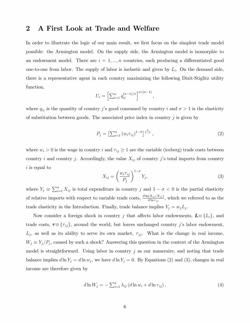
2 A First Look at Trade and Welfare

In order to illustrate the logic of our main result, we �rst focus on the simplest trade model

possible: the Armington model. On the supply side, the Armington model is isomorphic to

an endowment model. There are i = 1; :::; n countries, each producing a di¤erentiated good

one-to-one from labor. The supply of labor is inelastic and given by Li. On the demand side,

there is a representative agent in each country maximizing the following Dixit-Stiglitz utility

function,

Ui =hPn

i=1 q(��1)=�ij

i�=(��1),

where qij is the quantity of country j�s good consumed by country i and � > 1 is the elasticity

of substitution between goods. The associated price index in country j is given by

Pj =�Pn

i=1 (wi� ij)1��� 1

1�� , (2)

where wi > 0 is the wage in country i and � ij � 1 are the variable (iceberg) trade costs between

country i and country j. Accordingly, the value Xij of country j�s total imports from country

i is equal to

Xij =

�wi� ijPj

�1��Yj, (3)

where Yj �Pn

i=1Xij is total expenditure in country j and 1 � � < 0 is the partial elasticity

of relative imports with respect to variable trade costs, @ ln(Xij=Xjj)@ ln � ij

, which we referred to as the

trade elasticity in the Introduction. Finally, trade balance implies Yj = wjLj.

Now consider a foreign shock in country j that a¤ects labor endowments, L�fLig, and

trade costs, ��f� ijg, around the world, but leaves unchanged country j�s labor endowment,

Lj, as well as its ability to serve its own market, � jj. What is the change in real income,

Wj � Yj=Pj, caused by such a shock? Answering this question in the context of the Armington

model is straightforward. Using labor in country j as our numeraire, and noting that trade

balance implies d lnYj = d lnwj, we have d lnYj = 0. By Equations (2) and (3), changes in real

income are therefore given by

d lnWj = �Pn

i=1 �ij (d lnwi + d ln � ij) , (4)

6

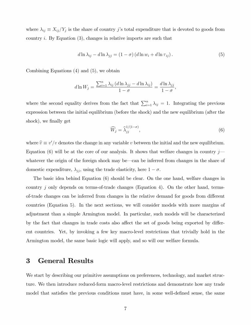
where �ij � Xij=Yj is the share of country j�s total expenditure that is devoted to goods from

country i. By Equation (3), changes in relative imports are such that

d ln�ij � d ln�jj = (1� �) (d lnwi + d ln � ij) . (5)

Combining Equations (4) and (5), we obtain

d lnWj =

Pni=1 �ij (d ln�jj � d ln�ij)

1� � =d ln�jj1� � ,

where the second equality derives from the fact thatPn

i=1 �ij = 1. Integrating the previous

expression between the initial equilibrium (before the shock) and the new equilibrium (after the

shock), we �nally get cWj = b�1=(1��)jj , (6)

where bv � v0=v denotes the change in any variable v between the initial and the new equilibrium.Equation (6) will be at the core of our analysis. It shows that welfare changes in country j�

whatever the origin of the foreign shock may be� can be inferred from changes in the share of

domestic expenditure, �jj, using the trade elasticity, here 1� �.

The basic idea behind Equation (6) should be clear. On the one hand, welfare changes in

country j only depends on terms-of-trade changes (Equation 4). On the other hand, terms-

of-trade changes can be inferred from changes in the relative demand for goods from di¤erent

countries (Equation 5). In the next sections, we will consider models with more margins of

adjustment than a simple Armington model. In particular, such models will be characterized

by the fact that changes in trade costs also a¤ect the set of goods being exported by di¤er-

ent countries. Yet, by invoking a few key macro-level restrictions that trivially hold in the

Armington model, the same basic logic will apply, and so will our welfare formula.

3 General Results

We start by describing our primitive assumptions on preferences, technology, and market struc-

ture. We then introduce reduced-form macro-level restrictions and demonstrate how any trade

model that satis�es the previous conditions must have, in some well-de�ned sense, the same

7

welfare predictions. Speci�c examples will be discussed in detail in Section 4.

3.1 Preferences, Technology, and Market Structure

We consider a world economy comprising i = 1; :::; n countries; one factor of production, labor;

and multiple goods indexed by ! 2 . We denote by N the measure of goods in .7 Labor is

inelastically supplied and immobile across countries. Li and wi denote the total endowment of

labor and the wage in country i, respectively.

Preferences. In each country i, there is a representative agent with Dixit-Stiglitz preferences

maximizing her utility subject to her budget constraint. The associated price index is given by

Pi =

�Z!2

pi(!)1��d!

� 11��

, (7)

where pi(!) is the price of good ! in country i and � > 1 is the elasticity of substitution between

goods. We adopt the convention that pi (!) = +1 if good ! is not available in country i.

Technology. For every good ! 2 , there is a blueprint that can be acquired by one or

many �rms depending on the market structure (to be described below). For any exporting

country i and any importing country j, the blueprint associated with good ! contains a set of

destination-speci�c techniques t 2 Tij that can be used to produce the good in country i and

sell it to country j. If a �rm from country i uses techniques t � ftjg to produce quantities

q � fqjg of good !, its cost function is given by

Ci (w; q; t; !) =Pn

j=1 [cij (wi; tj; !) qj + fij (wi; wj; tj; !) 1I(qj > 0)] ,

where w � fwjg is the vector of wages and 1I (�) is an indicator function. For each destination

country j, cij (wi; tj; !) > 0 is the constant marginal cost, which only requires labor in country i,

and fij (wi; wj; tj; !) � 0 is a �xed exporting cost, which may require labor in both the exporting

and importing countries. In line with the previous literature, we assume that constant marginal

7 may include either a discrete or a continuum of goods. Thus whenever the integral sign �R!2�appears,

one should think of a Lebesgue integral. If is a �nite or countable set, �R!2�is simply equivalent to �

P!2�.

This minor technicality allows us to cover the Armington model presented in Section 2. In practice, however,all other existing quantitative trade models comprise a continuum of goods.

8

costs and �xed exporting costs can be written as

cij (wi; tj; !) � � ij � wi � �ij (!) � t1

1��j ,

fij (wi; wj; tj; !) � �ij � hij(wi; wj) � �ij (!) �mij (tj) ,

where � ij � 1 and �ij > 0 are exogenous parameters common to all blueprints, which we will

use to parametrize changes in variable and �xed trade costs, respectively;8 hij(wi; wj) > 0 is a

homogenous of degree one function that captures the importance of domestic and foreign labor

in �xed exporting costs; �ij (!) > 0 and �ij (!) � 0 re�ect the exogenous heterogeneity across

blueprints; and mij (tj) � 0 re�ects endogenous destination-speci�c technological decisions. In

the rest of this paper, we assume that Tij ��t; t�, with t � 0 and t > 0, and that mij satis�es

m0ij > 0 andm

00ij < 0, which will guarantee the existence of a unique pro�t-maximizing technique

for all goods and all destinations. Since � > 1 and mij is increasing, higher t techniques imply

higher �xed exporting costs, but lower marginal costs.9

Market Structure. We consider two market structures: (i) perfect competition and (ii) mo-

nopolistic competition (with either restricted or free entry). Under both market structures,

there is a large number of �rms and all goods and labor markets clear. Under perfect competi-

tion, �rms have free access to all blueprints; there are no �xed exporting costs, �ij (!) = 0 for

all i, j, !; and all �rms maximize pro�ts taking wages and prices as given.

Under monopolistic competition with restricted entry, we assume that an exogenous mea-

sure of �rms, N i < N , freely receive monopoly power over a blueprint. Under monopolistic

competition with free entry, by contrast, �rms from country i need to hire Fi > 0 units of labor

in order to acquire monopoly power over a blueprint.10 The assignment of blueprints to �rms

8Despite this terminology, it should be clear that changes in variable trade costs may also capture productivitychanges: if � ij decrease by the same amount for all countries j = 1; :::; n, this is equivalent to an increase inlabor productivity in country i. Note also that in line with the existing literature, variable trade costs, whatevertheir origins may be, are modelled as cost- rather than demand-shifters.

9It is worth emphasizing that our assumptions on technology do not impose any restriction on the distributionof unit labor requirements, �ij (!), and �xed exporting costs, �ij (!), across goods. In particular, we allow thesedistributions to be degenerate. Thus monopolistically competitive models with homogeneous �rms, for example,are strictly covered by our analysis.10Under both restricted and free entry, each �rm gets monopoly power over only one blueprint. Thus, formally,

there are no multi-product �rms as in Bernard, Redding and Schott (2009) or Arkolakis and Muendler (2010).Extending our analysis to the case of multi-product �rms is trivial if there are no �xed trade costs at the �rm-level. Otherwise, our formal results would remain valid, but one would need to reinterpret the choice of whichproducts to sell in a particular destination as another destination-speci�c endogenous technological decision.

9

is random. The measure of goods Ni that can be produced in country i is then endogenously

determined so that entry costs, wiFi, are equal to expected pro�ts. Under both restricted and

free entry, we assume that once assigned a blueprint, �rms maximize pro�ts taking wages, total

expenditure, and consumer price indexes as given.

3.2 Macro-level Restrictions

We restrict ourselves to trade models satisfying three macro-level restrictions: (i) trade is

balanced; (ii) aggregate pro�ts are a constant share of GDP; and (iii) the �import demand

system is CES�. We now describe each restriction in detail.

Trade is balanced. As in Section 2, let Xij denote the total value of country j�s imports from

country i and let X �fXijg denote the n�n matrix of bilateral imports. Bilateral imports can

be expressed as

Xij =

Z!2ij

xij (!) d!, (8)

where ij � is the set of goods that country j buys from country i and xij (!) is the value of

country j�s imports of good ! from country i. Our �rst macro-level restriction is that the value

of imports must be equal to the value of exports:

R1 For any country j,Pn

i=1Xij =Pn

i=1Xji.

If �xed exporting costs are only paid in labor of the exporting country, R1 directly derives

from the budget constraint of country j�s representative agent. In general, however, total income

of the representative agent in country j may also depend on the wages paid to foreign workers by

country j�s �rms as well as the wages paid by foreign �rms to country j�s workers. Thus, total

expenditure in country j, Yj �Pn

i=1Xij, could be di¤erent from country j�s total revenues,

Rj �Pn

i=1Xji. R1 rules out this possibility. As in Section 2, we denote by �ij � Xij/Yj the

share of country j�s total expenditure that is devoted to goods from country i.

Aggregate pro�ts are a constant share of revenues. Let �j denote country j�s aggregate

pro�ts gross of entry costs (if any). Our second macro-level restriction states that �j must be

a constant share of country j�s total revenues:

R2 For any country j, �j=Rj is constant.

10

Under perfect competition, R2 trivially holds since aggregate pro�ts are equal to zero. Under

monopolistic competition with homogeneous �rms, R2 also necessarily holds because of Dixit-

Stiglitz preferences; see Krugman (1980). In more general environments, however, R2 is a

non-trivial restriction. We come back to this issue in Section 4.

The import demand system is CES. Our last macro-level restriction is concerned with the

partial equilibrium e¤ects of variable trade costs on aggregate trade �ows. As we later discuss in

Section 6, these are precisely the e¤ects that can be recovered from a simple gravity equation. To

introduce this last restriction formally, we de�ne the import demand system as the mapping from

(w;N ; � ) into X � fXijg, where w�fwig is the vector of wages, N � fNig is the vector of

measures of goods that can be produced in each country, and � � f� ijg is the matrix of variable

trade costs. This mapping is determined by utility and pro�t maximization given preferences,

technological constraints, and market structure.11 It excludes, however, labor market clearing

conditions as well as free entry conditions (if any) which determine the equilibrium values of w

andN . Broadly speaking, one can think of an import demand system as a set of labor demand

curves whose properties will be used to infer how changes in trade costs a¤ect the relative

demand for labor in di¤erent countries. Our third macro-level restriction imposes restrictions

on the partial elasticities, "ii0j � @ ln (Xij=Xjj)/ @ ln � i0j, of that system:

R3 The import demand system is such that for any importer j and any pair of exporters i 6= j

and i0 6= j, "ii0j = " < 0 if i = i0, and zero otherwise.

Each elasticity "ii0j captures the percentage change in the relative imports from country i in

country j associated with a change in the variable trade costs between country i0 and j holding

wages and the measure of goods that can be produced in each country �xed. According to

R3, like in a simple Armington model, any given change in bilateral trade costs, � ij, must have

a symmetric impact on relative demand, Xij=Xjj, for all exporters i 6= j. In addition, any

change in a third country trade costs, � i0j, must have the same proportional impact on Xij and

Xjj. Thus, changes in relative demand are separable across exporters: changes in the relative

11In principle, these equilibrium conditions may lead to multiple values of X for a given value of (w;N; � )if �rms from di¤erent countries have the same costs of producing and delivering a positive measure of goodsto the same destination under perfect competition or if a positive measure of �rms earn zero pro�ts (gross ofentry costs) under monopolistic competition. Both knife-edge scenarios, however, will be ruled out under ourthird-macro level restriction. At this point, if there are multiple values ofX, we arbitrarily select one, the choiceof the tie-breaking rule being of no consequence for the rest of our analysis.

11

demand for goods from country i, Xij=Xjj only depends on changes in � ij. When R3 is satis�ed

we say that the import demand system is CES and refer to " as the trade elasticity of that

system.12

A few comments are in order. First, the trade elasticity " is an upper-level elasticity: it

summarizes how changes in variable trade costs a¤ect aggregate trade �ows, whatever the

particular margins of adjustment, xij(!) or ij, may be. Below we will refer to the margin of

adjustment for trade �ows associated with xij(!) as the �intensive margin�and to the margin

of adjustment associated with ij as the �extensive margin�. Second, R3 is a global restriction

in that it requires the trade elasticity to be constant across all equilibria.13 Third, under perfect

competition, R3 implies complete specialization in the sense that for all i, i0 6= i, and j, the

measure of goods in ij\i0j must be equal to zero. Similarly, under monopolistic competition,

R3 implies that the measure of �rms that are indi¤erent about selling in a particular market

must be equal to zero. If these conditions were not true, at least one partial elasticity "ii0j would

be equal to+1. Finally, it is worth pointing out that although restrictions R1-R3 play a distinct

role in our analysis, they are not necessarily independent from one another. As we have shown

formally in the working paper version of this paper, Arkolakis, Costinot and Rodríguez-Clare

(2009), R3 implies R2 if �xed trade costs are only paid in labor of the exporting country.

In the rest of the paper we refer to models that satisfy the primitive assumptions introduced

in Section 3.1 as well as the macro-level restrictions R1-R3 as �quantitative trade models.�

For some of our results, we will use a stronger version of restriction R3:

R3�The import demand system is such that for any exporter i and importer j,

Xij =�ij �Ni � (wi� ij)

" � YjPni0=1 �i0j �Ni0 � (wi0� i0j)

" ,

12Our choice of terminology derives from the fact that in the case of a CES demand system, changes inrelative demand, Ck=Cl, for two goods k and l are such that @ ln (Ck=Cl)/ @ ln pk0 = 0 if k0 6= k; l and@ ln (Ck=Cl)/ @ ln pk = @ ln (Ck0=Cl)/ @ ln pk0 6= 0 for all k; k0 6= l. Nevertheless, it should be clear that theassumption of a CES import demand system is conceptually distinct from the assumption of CES preferences.While the import demand obviously depends on preferences, it also takes into account the supply side as thisa¤ects the allocation of expenditures to domestic production. In fact, CES preferences are neither necessary norsu¢ cient to obtain a CES import demand system.13This aspect of R3 is only necessary for our results to the extent that we are interested in the welfare

evaluation of arbitrary foreign shocks. A local version of R3 (i.e., assuming that R3 only holds at the initialequilibrium) would be su¢ cient to obtain a local version of our main result (i.e., one in which we characterizewelfare changes in response to in�nitesimally small shocks). We come back to this issue in Section 4.

12

where �ij is a function of, and only of, structural parameters distinct from � .

While R3�implies the same restriction on the partial elasticities "ii0j as R3, it further provides

a structural relationship between bilateral imports, wages, and the measure of goods that can

be produced in each country which we will exploit to predict changes in trade �ows.

3.3 Welfare valuation

We are interested in evaluating the changes in real income, Wj � Yj=Pj, associated with foreign

shocks in country j. To do so, we �rst introduce the following formal de�nition.

De�nition 1 A foreign shock in country j is a change from (L; F ; � ; �) to (L0; F 0; � 0; �0) such

that Lj = L0j, Fj = F0j, � jj = �

0jj, �jj = �

0jj, with L�fLig, F�fFig, � �f� ijg, and � �

��ij.

Put simply, foreign shocks correspond to any changes in labor endowments, entry costs,

variable trade costs, and �xed trade costs that do not a¤ect either country j�s endowment or

its ability to serve its own market.

Ex post welfare evaluation. We are now ready to state our �rst welfare prediction.

Proposition 1 Suppose that Restrictions R1-R3 hold. Then the change in real income associ-

ated with any foreign shock in country j can be computed as

cWj = b�1="jj . (9)

Proposition 1 o¤ers a parsimonious way to evaluate welfare changes resulting from foreign

shocks. One does not need to know the origins of the foreign shock or the way in which it

a¤ects trade �ows from di¤erent countries; it is su¢ cient to have information about the trade

elasticity, ", and the changes in trade �ows as summarized by b�jj.It is worth emphasizing that Proposition 1 is an ex post result in the sense that the per-

centage change in real income is expressed as a function of the change in the share of domestic

expenditure. Thus, it is only useful to the extent that b�jj is observed. For instance, lookingat historical trade data, Proposition 1 can be used to infer the welfare consequences of past

episodes of trade liberalization. However, it cannot be used to forecast the welfare consequences

13

of future episodes of trade liberalization, as di¤erent trade models satisfying Restrictions R1-

R3 may, in principle, predict di¤erent changes in the share of domestic expenditure for a given

foreign shock.

Ex ante welfare evaluation. We now turn to a very particular, but important type of

shock: moving to autarky. Formally, we assume that variable trade costs in the new equilibrium

are such that � 0ij = +1 for any pair of countries i 6= j. All other technological parameters

and endowments are the same as in the initial equilibrium. For this particular counterfactual

exercise, any trade model must predict the same change in the share of domestic expenditure:

�jj = 1=�jj since �0jj = 1 under autarky. Combining this observation with Proposition 1, we

immediately get:

Corollary 1 Suppose that Restrictions R1-R3 hold. Then the change in real income associated

with moving to autarky in country j can be computed as

cWAj = �

�1="jj . (10)

Unlike Proposition 1, Corollary 1 is an ex ante result in the sense that it does not require

any information on trade �ows in the new equilibrium. Conditional on initial values of �jj

and ", the gains from trade predicted by all models satisfying Restrictions R1-R3 must be

the same. Within that class of models, new margins of adjustment may a¤ect the structural

interpretation of the trade elasticity, and in turn, the composition of the gains from trade.

Nevertheless, new margins cannot change the total size of the gains from trade. The absolute

value of the percentage change in real income associated with moving from the initial equilibrium

to autarky remains given by 1� ��1=", as stated in the Introduction.

Ex-ante results can be derived for any change in variable trade costs if one strengthens our

third macro-level restriction from R3 to R3�.

Proposition 2 Suppose that Restrictions R1-R3� hold. Then the percentage change in real

income associated with any change in variable trade costs in country j can be computed using

Equation (9) combined with b�jj = 1Pni=1 �ij (wi� ij)

" , (11)

14

where wj = 1 by choice of numeraire, and fwigi6=j are implicitly given by the solution of

wi =Pn

j0=1

�ij0wj0Yj0 (wi� ij0)"

YiPn

i0=1 �i0j0 (wi0 � i0j0)" . (12)

Since Equations (11) and (12) only depend on trade data and the trade elasticity, Proposition

2 implies that the welfare consequences of any change in variable trade costs, not just moving

to autarky, must be the same in all trade models satisfying Restrictions R1-R3�.14

4 Examples

The main features of the trade models analyzed in Section 3 include four primitive assumptions:

(i) Dixit-Stiglitz preferences; (ii) one factor of production; (iii) linear cost functions; and (iv)

perfect or monopolistic competition; as well as three macro-level restrictions, which trivially

hold in a simple Armington model: (i) trade is balanced; (ii) aggregate pro�ts are a constant

share of aggregate revenues; and (iii) the import demand system is CES. In order to illustrate

the logic of our general results we now highlight two simple examples that satisfy our primitive

assumptions, but may or may not satisfy our macro-level restrictions: the Ricardian model and

the Melitz (2003) model.15 We �rst demonstrate how, like in a simple Armington model, one

can go from aggregate trade �ows to welfare predictions under our three macro-level restrictions.

We then discuss the exact role of our macro-level restrictions as well as the conditions under

which they hold in each environment.

4.1 The Ricardian Model

In this �rst example, we focus on perfect competition, abstract from endogenous technological

choices, t = t = 1, and assume that good-speci�c unit labor requirements do not vary across

14In the context of the Eaton and Kortum (2002) model, Dekle, Eaton and Kortum (2008) have previouslyshown that the change in trade �ows triggered by an arbitrary shock to variable trade costs can be entirelycharacterized in terms of the trade elasticity and the initial equilibrium trade �ows. The proof of the Propositionbuilds on Dekle, Eaton and Kortum (2008) approach and demonstrates that their result generalizes to anyquantitative trade model satisfying R1-R3�.15Whereas we do not focus on Krugman (1980) in this section, it should be clear that it satis�es our four

primitive assumptions as well as our three macro-level restrictions. In Krugman (1980), we simply have adegenerate distribution of unit labor requirements and �xed trade costs; R1 trivially holds in the absence of�xed exporting costs; and R2, R3 and R3�are direct implications of Dixit-Stiglitz preferences. Accordingly,Krugman (1980) leads to the same welfare predictions as a simple Armington model.

15

destinations, �ij (!) � �i (!). Under these assumptions, the general model presented in Section

3 reduces to a Ricardian model. Throughout this example, we denote by G (�1; :::; �n) the

share of goods ! 2 such that �i (!) � �i for all i, and by g (�1; :::; �n) the associated density

function.

Aggregate trade �ows. Under perfect competition, the set of goods ij that country j buys

from country i is given by

ij = f! 2 jcij�ij (!) < ci0j�i0j (!) for all i0 6= ig , (13)

where cij � wi� ij. Combining this observation with Dixit-Stiglitz preferences, we can write

aggregate trade �ows as

Xij =

R +10

(cij�i)1�� gi(�i; c1j; :::; cnj)d�iPn

i0=1

R +10

(ci0j�i0)1�� gi0(�i0 ; c1j; :::; cnj)d�i0

Yj, (14)

where gi(�i; c1j; :::; cnj) is the density of goods with unit labor requirements �i in ij.16 Ac-

cordingly, for any importer j and any pair of exporters i 6= j and i0 6= j, the import demand

system of a Ricardian model satis�es

@ ln (Xij=Xjj)

@ ln � i0j� "ii0j =

8<: 1� � + iij � ijj for i0 = i

i0ij � i

0jj for i0 6= i

, (15)

where 1�� and i0ij � @ lnhR +10

�1��i gi(�i; c1j; :::; cnj)d�i

i=@ ln ci0j are the intensive and exten-

sive margin elasticities, respectively.

Welfare predictions. Let us now demonstrate how the logic behind our welfare formula carries

over from the Armington to the Ricardian model. First, note that labor market clearing and

the budget constraint of the representative agent imply d lnYj = d lnwj = 0, where the second

equality derives from the choice of labor in country j as our numeraire. Thus, just as in the

Armington model, small changes in real income are given by

d lnWj = �d lnPj = �Pn

i=1 �ijd ln cij.

16Formally, gi(�i; c1j ; :::; cnj) �R�1>�icij=c1j

:::R�i�1>�icij=ci�1j

R�i+1>�icij=ci+1j

:::R�n>�icij=cnj

g (�) d��i,where �� (�1; :::; �n) and ��i denotes the previous vector with the i-th component removed.

16

The second equality re�ects the fact that under perfect competition, the welfare e¤ect of changes

at the extensive margin is necessarily second-order since consumers must be initially indi¤erent

between the �cuto¤�goods produced by di¤erent countries. By contrast, changes in trade �ows

now depend on changes in ij, and hence, the extensive margin elasticities, i0ij. In a Ricardian

model, by Equation (14), we have

d ln�ij � d ln�jj =�1� � + iij � ijj

�d ln cij +

Pni0 6=i;j

� i

0

ij � i0

jj

�d ln ci0j.

Combining the two previous expressions we get

d lnWj = �Pn

i=1 �ij

"d ln�ij � d ln�jj1� � + iij � ijj

�Pn

i0 6=i;j

i

0ij � i

0jj

1� � + iij � ijj

!d ln ci0j

#. (16)

To derive Proposition 1, we then simply note that Equation (15) and R3 imply i0ij = i

0jj for

all i0 6= i; j and 1� � + iij � ijj = " for all i 6= j. Together withPn

i=1 �ij = 1, Equation (16)

therefore implies d lnWj = d ln�jj=", which can be integrated to get cWj = b�1="jj .What is the role of our macro-level restrictions? R1 and R2 are trivially satis�ed

under perfect competition and do not play any active role in this environment. R3 is the

crucial restriction which guarantees that, as in a simple Armington model: (i) changes in each

component of the consumer price index, d ln cij, can be inferred one-by-one from changes in

relative imports, d ln�ij � d ln�jj (because i0ij = i

0jj for all i

0 6= i; j); (ii) changes in relative

imports can be aggregated into changes in the domestic share of expenditure, �d ln�jj (because

1��+ iij� ijj = " for all i 6= j); and (iii) small changes in the share of domestic expenditures

can be integrated into large ones (because the trade elasticity " is constant across equilibria).

The previous conditions are obviously strong. For instance, for condition (i) to hold, it must

be the case that third-country changes have symmetric e¤ects on country i and j, i.e. i0ij =

i0jj

for all i0 6= i; j. Thus R3 rules out, for example, a situation in which a decrease in bilateral

trade costs between Costa Rica and the United States has a di¤erential impact on Mexican and

Canadian exports to the United States. In the Armington model presented in Section 2, the

previous conditions were a direct implication of strong restrictions on the demand-side, namely

Dixit-Stiglitz preferences. For the same conditions to hold more generally in a Ricardian model,

we will need equally strong restrictions on the supply-side, as we now discuss.

17

When are our macro-level restrictions satis�ed? As Equation (15) shows, the import

demand system may not, in general, satisfy R3 because of the extensive margin elasticities,

i0ij. Eaton and Kortum�s (2002) well-known paper provides an example of a Ricardian model

satisfying R3. This model obtains as a particular case of our general model by assuming that

1=�i (!) are independently drawn from Fréchet distributions, i.e.

g (�1; :::; �n) �nYi=1

�Ti���1i e�Ti�

�i , for all �1; :::; �n � 0. (17)

Using the de�nition of i0ij and di¤erentiating Equation (14), we get

iij = � (� � � + 1)

Pi0 6=i �i0j

for i 6= j and i0ij = (� � � + 1)�i0j for i0 6= i; j. This implies that i

0ij = i

0jj = 0 for i0 6= i; j,

whereas " = 1 � � + iij � ijj = �� for i 6= j and thus R3 is satis�ed. Moreover, combining

Equations (17) and (14), we obtain

Xij =Ti (wi� ij)

��Pni0=1 Ti0 (wi0� i0j)

��Yj. (18)

Thus R3�is satis�ed as well. Accordingly, the welfare consequences of any change in variable

trade costs, not just moving to autarky, must be the same in Eaton and Kortum (2002) as in a

simple Armington model.

The comparison of these two models illustrates the main point of our paper in a very clear

manner. Since Eaton and Kortum (2002) entails production gains from trade whereas an

Armington model does not, one may think that the gains from trade predicted by Eaton and

Kortum (2002) must be larger. Our analysis demonstrates that this is not the case. As we switch

from an Armington model to Eaton and Kortum (2002), the structural interpretation of the

trade elasticity changes from a preference parameter, 1� �, to a technological parameter, ��,

re�ecting the fact there is now one more margin, namely ij, for bilateral imports to adjust.17

Yet, conditional on �jj and ", more margins of adjustment only a¤ect the composition of the

17While this is not the focus of our analysis, it is worth mentioning that the trade elasticity in Eaton andKortum (2002), " = ��, is independent of the intensive margin elasticity, 1��. This particular feature of Eatonand Kortum (2002) model can be explained as follows. On the one hand, changes in relative imports at theintensive margin are given by (1� �)d ln cij , just like in the Armington model. On the other hand, changes atthe extensive margin are given by (� � 1� �) d ln cij . By adding the e¤ects of these two margins, we obtaind ln�ij � d ln�jj = ��d ln cij . A similar feature has already been discussed in the context of the Melitz (2003)model by Chaney (2008), Arkolakis et al. (2008), and Feenstra (2009).

18

gains from trade, not their total size.

A natural question at this point is: Are there many other Ricardian models, beyond Eaton

and Kortum (2002), that satisfy R3? The short answer is: �Probably not.�The same way that

Dixit-Stiglitz preferences are crucial in guaranteeing the existence of a unique trade elasticity in

what boils down to a simple endowment economy in Section 2, it is hard to imagine R3 holding

in a Ricardian economy in the absence of very speci�c functional forms on the distribution of

unit labor requirements.18 That being said, it should be clear that, like in Section 2, functional

forms are only crucial for our results to the extent that we are interested in arbitrary shocks.

If only small shocks are considered, a simple example in which the import demand system is

locally CES� and hence a local version of Proposition 1 holds� is the case of a symmetric free

trade equilibrium. In this case, all extensive margin elasticities are equal, and so by Equation

(15), for any importer j and any pair of exporters i 6= j and i0 6= j, "ii0j = " < 0 if i = i0, and

zero otherwise.

4.2 The Melitz (2003) Model

We now turn to the case of monopolistic competition with free entry and �rm heterogeneity à

la Melitz (2003). This second example again abstracts from endogenous technological choices,

t = t = 1 (with mij (1) = 1), assumes that good-speci�c unit labor requirements do not vary

across destinations, �ij (!) � �i (!), and ignores heterogeneity in �xed costs, �ij (!) = 1 for

all i,j, !. Like in the Ricardian model, we denote by G (�1; :::; �n) the share of goods ! 2

such that �i (!) � �i for all i, and by g (�1; :::; �n) the associated density function. Finally, we

assume that exporting and importing country wages matter for �xed exporting costs through a

Cobb-Douglas function, hij(wi; wj) = w�i w

1��j , � 2 [0; 1].19

Aggregate trade �ows. Under monopolistic competition with Dixit-Stiglitz preferences, �rms

charge a constant markup, �= (� � 1), over marginal costs. The associated pro�ts (net of

�xed exporting costs) of a producer of good ! in country i selling in country j are thus given

by �ij (!) = [�cij�ij (!) = (� � 1)Pj]1�� (Yj=�) � �ijw�i w

1��j , where we again use the notation

18Wilson (1980) provides an early discussion of the relationship between Ricardian and endowment models.19Strictly speaking, the present example is more general than Melitz (2003) in that it allows for asymmetry

across acountries, as in Chaney (2008), and for marketing costs to be paid in multiple countries, as in Arkolakis(2010). The original Melitz (2003) model corresponds to the particular case in which � = 1.

19

cij � wi� ij. Denoting ��ij the cuto¤ determining the entry of �rms from country i in country

j, i.e. �ij (!) > 0 if and only if �ij (!) < ��ij, the set of goods ij that country j buys from

country i can be written as

ij =

8<:! 2 j�ij (!) < ��ij � � �1�� (� � 1)

�Pjcij

� �ijw

�i w

1��j

Yj

! 11��9=; . (19)

Combining this observation with Dixit-Stiglitz preferences, we get

Xij =NiR ��ij0 [cij�i]

1�� gi (�i) d�iPni0=1Ni0

R ��i0j

0 [ci0j�i0 ]1�� gi0 (�i0) d�i0

Yj, (20)

where the density gi (�i) of goods with unit labor requirements �i in ij is simply given

by the marginal density of g.20 Noting that @ ln��ij�@ ln � ij = @ ln��jj

�@ ln � ij � 1 and

@ ln��ij�@ ln � i0j = @ ln��jj

�@ ln � i0j if i0 6= i, the import demand system now satis�es

@ ln (Xij=Xjj)

@ ln � i0j= "ii

0

j =

8<: 1� � � ij +� ij � jj

� �@ ln��jj@ ln � ij

�for i0 = i�

ij � jj� � @ ln��jj

@ ln � i0j

�for i0 6= i

, (21)

where ij � d lnR ��ij0 �1��gi (�) d�

.d ln��ij is the counterpart of the extensive margin elastici-

ties under perfect competition.

Welfare predictions. As in the case of perfect competition, we now demonstrate how the logic

of Section 2 carries over from the Armington model to this richer environment provided that

R1-R3 hold. Under free entry, labor market clearing and the representative agent�s budget con-

straint still imply d lnYj = d lnwj = 0, where the second equality again derives from the choice

of labor in country j as our numeraire. A key di¤erence between this example and the previous

one is that changes in the consumer price index no longer satisfy d lnPj =Pn

i=1 �ijd ln cij, re-

�ecting the fact that, under monopolistic competition, consumers are not necessarily indi¤erent

between the �cuto¤� goods produced by di¤erent countries. Formally, small changes in real

20Formally, we now have gi (�i) =R�1�0 :::

R�i�1�0

R�i+1�0 ::::

R�n�0 g (�) d��i.

20

income are now given by

d lnWj = �d lnPj = �Pn

i=1 �ij

�d ln cij +

d lnNi + ijd ln��ij

1� �

�.

Using the de�nition of the cuto¤ ��ij this Equation can be rearranged as

d lnWj = �Pn

i=1

��ij

1� � � j

����1� � � ij

�d ln cij +

ij1� �

�d ln �ij + �d lnwi

�+ d lnNi

�,

where j �P

i �ij ij. Similarly, changes in trade �ows are now given by

d ln�ij�d ln�jj =�1� � � ij

�d ln cij+

ij1� �

�d ln �ij + �d lnwi

�+� ij � jj

�d ln��jj+d lnNi�d lnNj,

where we have used the fact that d ln��ij = d ln��jj � d ln cij +�d ln �ij + �d lnwi

�= (1� �).

Combining the two previous expressions reveals that

d lnWj = �Pn

i=1

��ij

1� � � j

���d ln�ij � d ln�jj �

� ij � jj

�d ln��jj + d lnNj

�.

Since R3 implies ij = jj and 1��� j = " for all i; j, we obtain d lnWj = (d ln�jj � d lnNj) =",

in the exact same way as in the previous example. To conclude, we simply note that free

entry implies �j = NjFj. Since �j is proportional to Yj by R1 and R2, we therefore have

d lnNj = d lnYj = 0. Combining the two previous observations and integrating, we again getcWj = b�1="jj .What is the role of our macro-level restrictions? Compared to the Ricardian model, R1

and R2 now play a substantial role. Together, they imply that aggregate pro�ts are a constant

share of total expenditure, which guarantees that the measure Nj of goods that can be produced

in country j is not a¤ected by foreign shocks.21 By contrast, R3 plays the exact same role as

in the Ricardian model, namely that small changes in each component of the consumer price

index can be inferred one-by-one from changes in relative imports, then aggregated into small

changes in the share of domestic expenditure, and �nally integrated into large changes to get

Proposition 1.

21Under restricted entry, R1 and R2 would play an analogous role by guaranteeing that aggregate pro�ts arenot a¤ected by foreign shocks; see proof of Proposition 1 in Appendix A.2.

21

Before discussing when R1-R3 hold, we wish to stress that the fact that Nj is not a¤ected by

foreign shocks� which is crucial for our welfare results� by no means implies that the measure

of goods consumed in country j is �xed. In particular, changes in both the foreign cuto¤s,

��ij, and the measure of goods that can be produced abroad, Ni, will a¤ect the number and

price of foreign goods consumed in country j. Hence our example allows for �gains from new

varieties� in the sense in which these gains are commonly measured; see e.g. Feenstra (1994)

and Broda and Weinstein (2006). Similarly, the fact that Nj is constant by no means implies

that foreign shocks have no e¤ect on intra-industry reallocations in country j. For instance, if

a given episode of trade liberalization increases the domestic cut-o¤, ��jj, the number of active

�rms in country j will decrease with labor being reallocated from the least to the most e¢ cient

�rms as documented in many micro-level studies; see e.g. Tre�er (2004).

When are our macro-level restrictions satis�ed? Under monopolistic competition, R1

and R2 are no longer trivial restrictions, as already mentioned in Section 3.2. Similarly, like

in a Ricardian model, R3 is unlikely to hold under monopolistic competition without strong

functional form restrictions.

By far the most common restriction on technology imposed in the literature on monopolistic

competition with �rm heterogeneity emanating from Melitz (2003) is that �rm-productivity

levels are randomly drawn from a Pareto distribution.22 Using our notations, the Pareto case

corresponds to a situation in which the marginal densities of g are such that

gi(�i) =����1i

�i�, for all 0 � �i � �i. (22)

If Equation (22) holds, our three macro-level restrictions are satis�ed. Using labor market

clearing, it is a simple matter of algebra to check that R1 and R2 are satis�ed. Using Equation

22Although not part of the original theoretical framework developed by Melitz (2003), this distributionalassumption is invoked, for example, in Antras and Helpman (2004), Helpman, Melitz and Yeaple (2004), Ghironiand Melitz (2005), Bernard, Redding and Schott (2007), Arkolakis (2010), Chaney (2008), Feenstra and Kee(2008), Hanson and Xiang (2008), Melitz and Ottaviano (2008), Feenstra (2009), Helpman and Itskhoki (2010),Di Giovanni and Levchenko (2010), Arkolakis and Muendler (2010), Helpman, Itskhoki and Redding (2010),Hsieh and Ossa (2010), and, as previously mentioned, in Eaton, Kortum and Kramarz (2010). While analyticalconvenience has clearly contributed to the popularity of Pareto distributions among trade economists, thereexist both empirical and theoretical reasons that favor this distributional assumption. As documented by Axtell(2001) and Eaton, Kortum, and Kramarz (2010), among others, Pareto distributions provide a reasonableapproximation for the right tail of the observed distribution of �rm sizes. From a theoretical standpoint, thesedistributions are also consistent with simple stochastic processes for �rm-level growth, entry, and exit; see e.g.Simon (1955), Gabaix (1999) and Luttmer (2007).

22

(22) and the de�nition of ij, it is also easy to check that ij = jj = 1� � + � and hence R3

is satis�ed with " = ��. Moreover, combining Equation (20), Equation (22), and the de�nition

of ��ij, we obtain

Xij =�i��Niw

����[ ���1�1]

i ��[ �

��1�1]ij ���ijPn

i0=1 �i0��Ni0w

����[ ���1�1]

i0 ��[ �

��1�1]i0j ���i0j

Yj. (23)

Interestingly, Equation (23) shows that whereas R3 always holds in the Pareto case, our stronger

macro-level restriction R3�is only satis�ed if � = 0, i.e. if �xed exporting costs are paid in the

importing country.23

Like in Section 4.1, the introduction of new margins of adjustment changes the structural

interpretation of the trade elasticity, ", from a preference parameter, 1 � �, to a technological

parameter, ��. Yet, because our three macro-level restrictions R1-R3 are satis�ed, the total

gains from trade can still be computed using only two statistics, �jj and ", as stated in Corollary

1. By contrast, because R3�no longer holds under monopolistic competition if � > 0, one would

need additional information, namely on � and �, to predict ex ante the welfare consequences

of an arbitrary change in variable trade costs. In such circumstances, the empirical approach

developed by Helpman, Melitz and Rubinstein (2008) could prove particularly useful since

it allows researchers to estimate separately the trade elasticity, ", and the intensive margin

elasticity, 1� �. We come back to estimation issues in Section 6.

We wish to be clear that R3 again requires strong functional form restrictions for inten-

sive and extensive margin elasticities �to behave in the same way.�Depending on the market

structure, perfect or monopolistic competition, we see that these functional form restrictions

are di¤erent, Fréchet or Pareto, re�ecting the di¤erent nature of selection into exports in these

environment; see Equations (13) and (19).24 In our view, the main advantage of R3 over par-

ticular functional form restrictions, such as Equations (17) and (22), is to provide a unifying

23This is the situation considered, for instance, in Eaton, Kortum and Kramarz (2010). Compared to theMelitz (2003) model presented in this section, Eaton, Kortum and Kramarz (2010) also includes heterogeneityin �xed costs and endogenous technology adoption, as formalized in Section 3. Using our notations, however,bilateral trade �ows in Eaton, Kortum and Kramarz (2010) also satisfy Equation (23) with � = 0, and therefore,R3�; see Equation (20), page 16 in Eaton, Kortum and Kramarz (2010).24Like under perfect competition, it should be clear that strong functional forms are only crucial to the extent

that we are interested in arbitrary shocks. For instance, if only small foreign shocks are considered and the initialtrade equilibrium is fully symmetric, then the import demand system always is locally CES. If, in addition, �xedexporting costs are paid in domestic labor (� = 0), this immediately implies that a local version of Proposition1 holds as well (since R1 and R2 necessarily hold in this case).

23

perspective on the economic mechanisms responsible for the equivalence across quantitative

trade models, independently of their market structure.

5 Extensions

In this section we brie�y discuss how our results would be a¤ected by departures from the

primitive assumptions imposed in Section 3.1. Motivated by the existing trade literature, we

consider extensions of quantitative trade models with multiple sectors, as in Chor (2010), Don-

aldson (2008), Costinot, Donaldson and Komunjer (2010), and Caliendo and Parro (2010) and

tradable intermediate goods, as in Eaton and Kortum (2002), Alvarez and Lucas (2007), Waugh

(2010), Atkeson and Burstein (2010) and Di Giovanni and Levchenko (2009). We conclude by

mentioning other extensions such as multiple factors of production and variable mark-ups. A

detailed analysis of the extensions to multiple sectors and tradable intermediate goods can be

found in the online appendix. Here we limit ourselves to a summary of our main �ndings.

5.1 Multiple Sectors

It is standard to interpret models with Dixit-Stiglitz preferences, such as the one presented

in Section 3.1, as �one-sector�models with a continuum of �varieties�; see e.g. Helpman and

Krugman (1985). Under this interpretation, our model can be extended to multiple sectors,

s = 1; :::; S, by assuming that the representative agent has a two-tier utility function, with the

upper-tier being Cobb-Douglas, with consumption shares 0 � �s � 1, and the lower-tier being

Dixit-Stiglitz with elasticity of substitution �s > 1. In this case, the consumer price index in

country j becomes Pj =QSs=1

�P sj��s, where P sj is the Dixit-Stiglitz price index associated with

varieties from sector s, as described in Equation (7).

Assuming that technology and market structure remain as described in Section 3.1 and

that our three macro-level restrictions now hold sector-by-sector,25 the change in real income

25For R2 and R3, we simply mean that our macro-level restrictions now apply to �sj , Rsj , and

�Xsij

. In

the case of R1, we do not mean that trade is balanced sector-by-sector, which would not be true in modelsconsidered in the literature. Rather we mean that wjLsj + �

sj � wjNs

j Fsj = R

sj �

Pni=1X

sji for all s = 1; :::; S.

This restriction is the sector-by-sector version of R1 when we write this restriction for the one-sector environmentas wjLj + �j � wjNjFj = Rj , which is of course equivalent to trade balance given the representative agent�sbudget constraint in country j.

24

associated with an arbitrary foreign shock generalizes to:

cWj =QSs=1

�b�sjj��sj/"s , under perfect competition,

cWj =QSs=1

��s

jj

. bLsj��sj/"s , under monopolistic competition with free entry,

where �sjj � 0 represents the share of expenditure devoted to domestic goods in sector s; and

"s < 0 and Ls � 0 are the trade elasticity and total employment in that sector, respectively.

The new formula under perfect competition is a straightforward generalization of Proposition 1,

and requires no explanation. To understand the appearance of bLsj in our welfare formula undermonopolistic competition with free entry, it is useful to go back to the example of Section 4.2. In

that case, R3 implied that the welfare e¤ect of a foreign shock was given by cWj =�b�jj= bNj�1=".

But since the supply of labor was inelastic, Restrictions R1 and R2 lead to bNj = bLj = 1,

and so, cWj = b�1="jj . By contrast, in a multi-sector environment, the supply of labor in eachsector is no longer inelastic: foreign shocks may lead to changes in sector-level employment

with consequences for the measure of goods that can be produced, i.e. bN sj = bLsj 6= 1. This is

the key idea behind our generalized formula.26

Compared to the results presented in Section 3, we see that the welfare consequences of

foreign shocks, in general, and the gains from trade, in particular, may no longer be the same

under perfect and monopolistic competition with free entry. As our previous discussion empha-

sized, the equivalence between these two classes of quantitative trade models relied on the fact

that there was no change in the measure of goods Nj that can be produced in country j, which

may no longer be true in all sectors.27 That being said, it is important to note that there is no

particular reason for gains from trade to be higher (or lower) under monopolistic than under

perfect competition. Although gains from trade are larger in sectors in which the set of goods

that can be produced expands, bN sj > 0, they are lower in those in which it contracts, bN s

j < 0,

the overall e¤ect depending on whetherQSs=1

�bLsj��sj/"s is higher or lower than one.26The same logic implies that our welfare formula under monopolistic competition with restricted entry would

be exactly the same as under perfect competition.27In a related paper, Balistreri, Hillberry and Rutherford (2009) have developed variations of the Armington

and Melitz (2003) models with a non-tradeable sector to illustrate the same idea: if changes in trade costs lead tochanges in the measure of goods that can be produced, then models with perfect and monopolistic competitionno longer have the same welfare implications.

25

5.2 Tradable Intermediate Goods

In Section 3 all goods were for �nal consumption. In this extension we allow goods ! 2 to be

used in the production of other goods. Formally, we assume that all goods can be aggregated

into a unique intermediate good using the same Dixit-Stigliz aggregator as for �nal consumption.

Thus, Pi now represents both the consumer price index in country i and the price of intermediate

goods in this country. Accordingly, the cost function for each good ! is given by

Ci (w;P ; q; t; !) =Pn

j=1 [cij (wi; Pi; tj; !) qj + fij (wi; Pi; wj; Pj; tj; !) 1I(qj > 0)] ,

where P � fPig is the vector of intermediate good prices. In line with the previous literature

we further assume that constant marginal costs and �xed exporting costs can be written as

cij (wi; Pi; tj; !) � � ij � w�i � P1��i � �ij (!) � t

11��j ,

fij (wi; Pi; wj; Pj; tj; !) � �ij � hij(w�i P

1��i ; w�j P

1��i ) � �ij (!) �mij (tj) ,

with � 2 [0; 1] governing the share of intermediate goods in variable and �xed production costs.

Similarly, we assume that �xed entry costs (if any) are given by w�i P1��i Fi, with � 2 [0; 1]

governing the share of intermediate goods in entry costs. In this environment the change in real

income associated with an arbitrary foreign shock in country j generalizes to:

cWj = b�1/"�jj , under perfect competition,cWj = b�1/["��(1��)( "��1+1)+(1��)]

jj , under monopolistic competition with free entry,

where " now refers to the trade elasticity of the import demand system de�ned as a mapping from

(w;P ;N ; � ) into X.28 Under perfect competition, the fact that tradable intermediate goods

are used to produce tradable intermediate goods creates an input-output loop that ampli�es

the gains from trade. The higher the share of intermediate goods in production (i.e., the lower

is �), the higher this ampli�cation e¤ect. Under monopolistic competition with free entry there

are two additional ampli�cation mechanisms associated with the decrease in �xed exporting

28This generalization of the de�nition of the import demand system re�ects the fact that there are now twoinputs in production, labor and the aggregate intermediate goods, with prices given by w and P , respectively.

26

and entry costs, both of which increase the number of consumed varieties in country j.29 The

second of these ampli�cation mechanisms is reminiscent of the e¤ect of trade on growth in the

�lab equipment�model; see Rivera-Batiz and Romer (1991).

Just as in the case of multiple sectors, we see that our welfare formula is no longer the

same under perfect and monopolistic competition. There is, however, an important di¤erence

between our two extensions. In the case of multiple sectors, the e¤ect of trade on entry under

monopolistic competition could either lead to higher or lower gains from trade. This is no longer

the case here: the gains from trade are unambiguously larger under monopolistic than perfect

competition.

5.3 Other Extensions

We end this section by mentioning two additional extensions: multiple factors of production and

variable mark-ups. A simple way to introduce multiple factors of production into our general

framework is to assume that: (i) there are multiple sectors, as in Section 5.1; (ii) all goods from

the same sector have the same factor intensity; but (iii) factor intensity di¤ers across sectors;

see e.g. Bernard, Redding and Schott (2007) and Burstein and Vogel (2010). Under perfect

competition, the reasoning presented in the previous sections remains valid up to a point: the

formula in Proposition 1 now needs to be augmented to re�ect changes in relative factor prices

domestically. This is because sector-level trade �ows cannot tell us what is fundamentally an

economy-wide impact of trade on factor prices. Under monopolistic competition, this issue is

complicated by the implications of trade for the measure of goods that can be produced in

di¤erent sectors, as discussed earlier.30

Throughout this paper, we have focused on trade models with constant mark-ups, either

because of perfect competition or monopolistic competition with Dixit-Stiglitz preferences. Al-

lowing for quasi-linear preferences or translog expenditure functions, as in Melitz and Ottaviano

29Under monopolistic competition with free entry, Equation (23) shows that a decline in the �xed cost of

serving the domestic market��jj�increases the domestic trade share (�jj) with an elasticity �

�"

��1 + 1�while

a decline in the entry cost (Fj) increases �jj with a unitary elasticity. The term � (1� �)�

"��1 + 1

�+ (1� �)

inside the bracket in the welfare formula above follows from the fact that a decline in Pj decreases the �xedtrade cost and the entry cost with elasticities 1� � and 1� �, respectively.30These complications notwithstanding, explicit welfare formulas can still be obtained in the case of Cobb-

Douglas production functions, as demonstrated formally in Arkolakis, Costinot and Rodríguez-Clare (2009).

27

(2008) and Feenstra and Weinstein (2009), or Bertrand competition, as in Bernard, Eaton,

Jensen and Kortum (2003), would introduce variations in mark-ups, and hence, a new source of

gains from trade. While the introduction of these pro-competitive e¤ects, which falls outside the

scope of the present paper, would undoubtedly a¤ect the composition of the gains from trade,

our formal analysis is a careful reminder that it may not a¤ect their total size. In fact, it is easy

to check that in Bernard et al. (2003), our simple welfare formula remains unchanged in spite

of variable mark-ups at the �rm-level. The same is true under monopolistic competition with

translog expenditure functions if �rm productivity levels are drawn from a Pareto distribution,

as shown in Arkolakis, Costinot and Rodriguez-Clare (2010).

6 Estimating the Trade Elasticity

In the previous sections, we have demonstrated how the welfare implications of quantitative

trade models, as de�ned in Section 3, crucially depend on two su¢ cient statistics: (i) the share

of expenditure on domestic goods, �jj; and (ii) the trade elasticity, ". While the �rst of these

two statistics can be readily computed from o¢ cial statistics, the second cannot. The trade

elasticity needs to be estimated and this estimation may, in principle, depend on the details of

the model. Put simply, whereas all quantitative trade models imply that the gains from trade

are equal to 1���1=", our analysis so far leaves open the possibility that the estimate of " itself

is model speci�c.

In this section we will argue that, in spite of the di¤erent possible structural interpretations

of the trade elasticity in the class of models considered in this paper, this is, to a large extent,

not the case. Independently of their micro-level predictions, the �gravity equation� o¤ers a

common way to estimate the trade elasticity across di¤erent quantitative trade models, and

therefore, together with Corollary 1, a common estimator of the gains from trade.

There is more than one formal de�nition of the �gravity equation�in the trade literature.

Here we adopt a fairly broad de�nition, consistent with Anderson (2010), and say that a trade

model satis�es a gravity equation if it predicts that in any cross-section, bilateral imports can

be decomposed into:

lnXij = Ai +Bj + ln � ij + �ij, (24)

28

where Ai is an exporter-speci�c term; Bj is an importer-speci�c term; is the partial elasticity

of bilateral imports with respect to variable trade costs; and �ij captures country-pair speci�c

parameters that are distinct from variable trade costs (if any). Under standard orthogonality

conditions, Equation (24) o¤ers a simple way to estimate using observed measures of bilateral

imports and variable trade costs; see e.g. Anderson and Van Wincoop (2004).

Given the previous de�nition, it is immediate that a quantitative trade model satisfying

R3�also satis�es gravity with the partial elasticity of bilateral imports being equal to the

trade elasticity ".31 Thus, within this class of models, provided that the same orthogonality

condition is invoked, gravity o¤ers a common estimator of the trade elasticity, and in turn, of

the overall gains from trade. What if a quantitative trade model does not satisfy R3�? In this

situation, bilateral trade �ows may not, in principle, satisfy gravity as de�ned in Equation (24).

For existing quantitative trade models, however, bilateral imports can always� to the best of

our knowledge� be decomposed into Xij =�ij �Ni�w"

0i ��"ij �YjPn

i0=1 �i0j �Ni0 �w"0i0 ��

"i0j. Although R3�is not satis�ed if

"0 6= ", it is still the case that " can be recovered from a simple gravity equation.32 Thus, within

that extended class of models, there remains a common estimator of the gains from trade.

As hinted above, a key issue for a common estimator of the gains from trade to exist is that

the same orthogonality condition can be invoked across di¤erent models. In our view, this issue

is primarily an econometric one, which we have little to contribute to. To be more speci�c,

suppose that variable trade costs are being measured using tari¤ data; see e.g. Baier and

Bergstrand (2001).33 In order to obtain unbiased estimates of " using a gravity equation, one

needs tari¤s to be uncorrelated with the error term associated with Equation (24). Although it

is true that this error term may have a di¤erent structural interpretation in di¤erent models�

and in particular, that it may re�ect �xed trade costs under monopolistic competition� the

central question remains an econometric one, namely: is the observed component of trade costs

uncorrelated with its unobserved component? If so, there will be omitted variable bias, whatever

the economic nature of the unobserved component may be.

31Formally, if a trade model satis�es R3� then it satis�es Equation (24) with �i = lnNi + " lnwi; �j =lnYj � ln [

Pni0=1Ni0 � (wi0� i0j)

"]; = "; and �ij = ln�ij .

32An example of a quantitative trade model with "0 6= " is the Melitz (2003) model presented in Section 4.2 ifthe share of domestic labor in �xed exporting costs � is di¤erent from zero.33To the extent that they act as cost-shifters, tari¤s can be used, like any other variable trade costs, to obtain

estimates of the trade elasticity using a gravity equation. By contrast, our main welfare formula would need tobe modi�ed to cover the case of tari¤s. In particular, the results derived in Section 3 ignore changes in tari¤revenues, which may a¤ect real income both directly and indirectly (through the entry and exit of �rms).

29

Although the gravity equation o¤ers a common estimator of the trade elasticity, we wish

to emphasize that it does not o¤er, in general, the unique estimator of that elasticity. For

example, in the Melitz (2003) model presented in Section 4.2, the trade elasticity is equal to the

(negative of the) shape parameter of the Pareto distribution of �rm-level productivity. Since

this Pareto parameter also a¤ects the distribution of �rm sales, one can then use micro-level

data to estimate "; see e.g. Di Giovanni and Levchenko (2009). Given the distance between the

assumptions needed to estimate parameters from micro data and the key features of aggregate

models, however, such an approach is not without its problems; see Heckman and Hansen

(1996) for an overview. For the central question in this paper, �how large are the gains from

trade?�, our view is that estimating the trade elasticity using a gravity equation is a particularly

attractive procedure since, by its very nature, it captures by how much aggregate trade �ows,

and therefore consumption, reacts to changes in trade costs.

7 Concluding Remarks

What conclusions should one draw from our theoretical analysis? In our view, two broad

messages emerge from our equivalence results.

The �rst message is a cautionary one. Although it may be tempting to think that new

and richer quantitative trade models necessarily entail larger gains from trade, our analysis

demonstrates that this is not the case. Within the class of trade models considered in this

paper, the number of sources of gains from trade varies, but conditional on observed trade data,

the total size of the gains from trade does not. Of course, our equivalence results do not aim

to suggest that micro-level data cannot be useful for thinking about the welfare implications

of international trade. Rather, our point is that for micro-level data to a¤ect estimates of the

gains from trade, these data will have to be used in combination with trade models that fall

outside the scope of the present paper, hence our �So far, not much�in the Introduction.

The second message is more positive. The �ip side of our strong equivalence results is that

within a particular but important class of trade models, there exist two su¢ cient statistics for

welfare analysis: (i) the share of expenditure on domestic goods; and (ii) the trade elasticity.

Although quantitative trade models are now able to explain a wider set of micro-level facts,

they can still be used for counterfactual analysis using a very limited amount of macro data,

30

thereby preserving one of the most attractive features of the simple Armington model.

31

References

Alvarez, Fernando and Robert E. Lucas. 2007. �General Equilibrium Analysis of the Eaton-Kortum

Model of International Trade.�Journal of Monetary Economics 54(6):1726�1768.

Anderson, James E. 1979. �A Theoretical Foundation for the Gravity Equation.� The American

Economic Review 69(1):106�116.

Anderson, James E. 2010. �The Gravity Model.� forth. Annual Review of Economics .

Anderson, James E. and Eric Van Wincoop. 2003. �Gravity with Gravitas: A Solution to the Border

Puzzle.�The American Economic Review 93(1):170�192.

Anderson, James E. and Eric Van Wincoop. 2004. �Trade Costs.� Journal of Economic Literature

42(3):691�751.

Antras, Pol and Elhanan Helpman. 2004. �Global Sourcing.�Journal of Political Economy 112(3):552�

580.

Arkolakis, Costas. 2010. �Market Penetration Costs and the New Consumers Margin in International

Trade.� forthcoming, Journal of Political Economy .

Arkolakis, Costas, Arnaud Costinot and Andres Rodríguez-Clare. 2009. �New Trade Models, Same

Old Gains?�NBER Working Paper 15628.

Arkolakis, Costas, Arnaud Costinot and Andres Rodriguez-Clare. 2010. �Gains From Trade under

Monopolistic Competition: A Simple Example with Translog Expenditure Functions and Pareto

Distributions of Firm-Level Productivity.�. Manuscript, MIT, Penn State, and Yale University.

Arkolakis, Costas and Marc-Andreas Muendler. 2010. �The Extensive Margin of Exporting Products:

A Firm-Level Analysis.�NBER Working Paper 16641.

Arkolakis, Costas, Svetlana Demidova, Peter J Klenow and Andres Rodríguez-Clare. 2008. �Endoge-

nous Variety and the Gains from Trade.� American Economic Review, Papers and Proceedings

98(4):444�450.

Atkeson, Andrew and Ariel Burstein. 2010. �Innovation, Firm Dynamics, and International Trade.�

Journal of Political Economy 118(3):433�489.

Axtell, Rob L. 2001. �Zipf Distribution of U.S. Firm Sizes.�Science 293(5536):1818�1820.

32

Baier, Scott L. and Je¤rey H. Bergstrand. 2001. �The Growth of World Trade: Tari¤s, Transport

Costs, and Income Similarity.�Journal of International Economics 53(1):1�17.

Balistreri, Edward J., Russell H. Hillberry and Thomas F. Rutherford. 2009. �Trade and Welfare:

Does Industrial Organization Matter.�. Manuscript, University of Melbourne.

Bernard, Andew B., Jonathan Eaton, J. Bradford Jensen and Samuel Kortum. 2003. �Plants and

Productivity in International Trade.�The American Economic Review 93(4):1268�1290.

Bernard, Andrew B., Stephen J. Redding and Peter Schott. 2007. �Comparative Advantage and

Heterogeneous Firms.�Review of Economic Studies 74(1):31�66.

Bernard, Andrew B., Stephen J. Redding and Peter Schott. 2009. �Multi-Product Firms and Trade

Liberalization.�NBER Working Paper 12782.

Broda, Cristian and David Weinstein. 2006. �Globalization and the Gains from Variety.�Quarterly

Journal of Economics 121(2):541�585.

Burstein, Ariel and Jonathan Vogel. 2010. �Globalization, Technology, and the Skill Premium.�.

Manuscript, Columbia University and UCLA.

Caliendo, Lorenzo and Fernando Parro. 2010. �Estimates of the Trade andWelfare E¤ects of NAFTA.�.

Manuscript, University of Chicago.

Chaney, Thomas. 2008. �Distorted Gravity: The Intensive and Extensive Margins of International

Trade.�The American Economic Review 98(4):1707�1721.

Chetty, Raj. 2009. �Su¢ cient Statistics for Welfare Analysis: A Bridge Between Structural and

Reduced-Form Methods.�Annual Review of Economics 1:451�488.

Chor, Davin. 2010. �Unpacking Sources of Comparative Advantage: A Quantitative Approach.�forth.

Journal of International Economics .

Costinot, Arnaud, Dave Donaldson and Ivana Komunjer. 2010. �What Goods Do Countries Trade? A

Quantitative Exploration of Ricardo�s Ideas.�. Manuscript, MIT.

Dekle, Robert, Jonathan Eaton and Samuel Kortum. 2008. �Global Rebalancing with Gravity: Mea-

suring the Burden of Adjustment.�IMF Sta¤ Papers 55(3):511�540.

33

Di Giovanni, Julian and Andrei A. Levchenko. 2009. �Firm Entry, Trade, andWelfare in Zipf�s World.�.

Manuscript, University of Michigan.

Donaldson, Dave. 2008. �Railroads of the Raj: Estimating the Economic Impact of Transportation

Infrastructure.�. Manuscript, London School of Economics.

Eaton, Jonathan and Samuel Kortum. 2002. �Technology, Geography and Trade.� Econometrica

70(5):1741�1779.

Eaton, Jonathan, Samuel Kortum and Francis Kramarz. 2010. �An Anatomy of International Trade:

Evidence from French Firms.�NBER Working Paper 14610.

Feenstra, Robert. 1994. �New Product Varieties and the Measurement of International Prices.�The

American Economic Review 84(1):157�177.

Feenstra, Robert. 2009. �Measuring the Gains from Trade under Monopolistic Competition.�. Manu-

script, University of California, Davis.

Feenstra, Robert and David Weinstein. 2009. �Globalization, Competition, and the U.S. Price Level.�.

Manuscript, University of California, Davis and Columbia University.

Feenstra, Robert and Hiau Looi Kee. 2008. �Export Variety and Country Productivity: Estimat-

ing the Monopolistic Competition Model with Endogenous Productivity.�Journal of International

Economics 74(2):500�518.

Gabaix, Xavier. 1999. �Zipf�s Law for Cities: An Explanation.� Quarterly Journal of Economics

114(3):739�767.

Ghironi, F. and M.J. Melitz. 2005. �International Trade and Macroeconomic Dynamics with Hetero-

geneous Firms.�Quarterly Journal of Economics 120(3):865�915.

Goldberg, P., A. Khandelwal, Nina Pavcnik and P. Topalova. 2009. �Trade Liberalization and New

Imported Inputs.�American Economic Review, Papers and Proceedings 99(2):494�500.

Hanson, Gordon and Chong Xiang. 2008. �Testing the Melitz Model: An Application to US Motion

Picture Exports.�NBER Working Paper 14461.

Heckman, James J. and Lars Peter Hansen. 1996. �The Empirical Foundations of Calibration.�Journal

of Economic Perspectives 10(1):87�104.

34

Helpman, Elhanan, Marc J. Melitz and Stephen R. Yeaple. 2004. �Export Versus FDI with Heteroge-

neous Firms.�The American Economic Review 94(1):300�316.

Helpman, Elhanan, Marc Melitz and Yona Rubinstein. 2008. �Estimating Trade Flows: Trading

Partners and Trading Volumes.�Quarterly Journal of Economics 2(5):441�487.

Helpman, Elhanan and Oleg Itskhoki. 2010. �Labor Market Rigidities, Trade and Unemployment.�

Review of Economic Studies 77(3):1100�1137.

Helpman, Elhanan, Oleg Itskhoki and Stephen J. Redding. 2010. �Inequality and Unemployment in a

Global Economy.�Econometrica 78(4):1239�1283.

Helpman, Elhanan and Paul Krugman. 1985. Market Structure and Foreign Trade: Increasing Returns,

Imperfect Competition, and the International Economy. Cambridge, Massachusetts: MIT Press.

Hsieh, Chang-Tai and Ralph Ossa. 2010. �A Global View of Productivity Growth in China and India.�.

mimeo, University of Chicago.

Klenow, Peter J. and Andres Rodríguez-Clare. 1997. �Quantifying Variety Gains from Trade Liberal-

ization.�. Manuscript, University of Chicago.

Krugman, Paul. 1980. �Scale Economies, Product Di¤erentiation, and the Pattern of Trade.�The

American Economic Review 70(5):950�959.

Luttmer, Erzo G. J. 2007. �Selection, Growth, and the Size Distribution of Firms.�Quarterly Journal

of Economics 122(3):1103�1144.

Melitz, Marc J. 2003. �The Impact of Trade on Intra-Industry Reallocations and Aggregate Industry

Productivity.�Econometrica 71(6):1695�1725.

Melitz, Marc J. and Gianmarco I. P. Ottaviano. 2008. �Market Size, Trade, and Productivity.�The

Review of Economic Studies 75(1):295�316.

Norihiko, Yamano and Nadim Ahmad. 2006. �The OECD Input-Output Database: 2006 Edition.�

Working Paper 2006/8, OECD .

Rivera-Batiz, Luis A. and Paul M. Romer. 1991. �International Trade with Endogenous Technological

Change.�European Economic Review 95(971-1001):971�1001.

Simon, Herbert A. 1955. �On a Class of Skew Distribution Functions.�Biometrika 42(3/4):425�440.

35

Tre�er, Daniel. 2004. �The Long and Short of the Canada-US Free Trade Agreement.� American

Economic Review 94(4):870�895.

Waugh, Mike. 2010. �International Trade and Income Di¤erences.� forthcoming, American Economic

Review .

Wilson, Charles A. 1980. �On the General Structure of Ricardian Models with a Continuum of Goods:

Applications to Growth, Tari¤ Theory, and Technical Change.�Econometrica 48(7):1675�1702.

36

A Proof of Proposition 1Throughout this Appendix, for any importing country j, we denote by Gj (�1; :::; �n; �1; :::; �n) theshare of goods ! 2 such that �ij (!) � �i and �ij (!) � �i for all i, and by gj (�1; :::; �n; �1; :::; �n)the associated density function. For expositional purposes, we provide separate proofs of Proposition1 for perfect and monopolistic competition.

A.1 Perfect CompetitionUnder perfect competition, it is convenient to use the following additional notations:

cij � wi� ijt1

1�� , (A1)

gij(�i; c1j ; :::; cnj) �R�1>

�icijc1j

:::R�i�1>

�icijci�1j

R�i+1>

�icijci+1j

:::R�n>

�icijcnj

gj (�; 0) d��i, (A2)

where �� (�1; :::; �n), 0� (0; :::; 0), and ��i denotes the vector � with the i-th component removed.In order to establish Proposition 1, we will make use of the following lemma which characterizes

the consumer price index, Pj , and the share of expenditure, �ij , on goods from country i in country junder perfect competition.

Lemma 1 Suppose that R3 holds. Then under perfect competition, Pj and �ij satisfy

Pj =

�Pni=1

Z +1

0(cij�i)

1��Ngij(�i; c1j ; :::; cnj)d�i

� 11��

, (A3)

�ij =

R +10 (cij�i)

1�� gij(�i; c1j ; :::; cnj)d�iPni0=1

R +10

�ci0j�i0

�1��gi0j(�i0 ; c1j ; :::; cnj)d�i0

, (A4)

Proof. As pointed out in Section 3.2, there must be complete specialization under R3. Thus we canexpress the price index and shares of expenditure, respectively, as

Pj =

"Pni=1

Z!2ij

pj(!)1��d!

# 11��

, (A5)

�ij =

R!2ij pj(!)

1��d!Pni0=1

R!2i0j

pj(!)1��d!, (A6)

where Equation (A6) directly follows from Equation (A5) and Shephard�s Lemma. Under perfectcompetition, there are no �xed costs and all �rms from country i have free access to all blueprints.Thus pro�t-maximization implies

pj(!) = cij�ij (!) , for all ! 2 ij , (A7)

withij =

�! 2 jcij�ij (!) < ci0j�i0j (!) for all i0 6= i

, (A8)

37

where cij is given by Equation (A1). Note that since the measure of goods for which cij�ij (!) =ci0j�i0j (!) for i0 6= i must be zero under complete specialization, the strict inequality in Equation (A8)is without any loss of generality. Together with the de�nition of gij(�i; c1j ; :::; cnj) in Equation (A2),Equations (A5)-(A8) immediately imply Equations (A3) and (A4). QED.

We are now ready to establish Proposition 1 under perfect competition.

Proof of Proposition 1 (Perfect competition). We proceed in �ve steps. Throughout this proofwe use labor in country j as our numeraire, wj = 1.

Step 1: Small changes in real income satisfy

d lnWj = �d lnPj . (A9)

By de�nition, we know that d lnWj = d lnYj � d lnPj . By labor market clearing and the represen-tative agent�s budget constraint, we also know that d lnYj = d lnwj . Equation (A9) directly followsfrom these two observations and the fact that d lnwj = 0, by our choice of numeraire.

Step 2: Small changes in the consumer price index satisfy

d lnPj =Pni=1 �ijd ln cij . (A10)

By Lemma 1, we know that the consumer price index is given by Equation (A3). Totally di¤erentiatingthis expression, we obtain

d lnPj =

�1

1� �

��Pni=1 �ij

h(1� �) d ln cij +

Pni0=1

i0ijd ln ci0j

i, (A11)

where

i0ij �

@ ln�R +10 �1��i gij(�i; c1j ; :::; cnj)d�i

�@ ln ci0j

.

By Equation (A2), the extensive margin elasticities satisfy iij = �Pi0 6=i

i0ij . Thus we can rewrite

Equation (A11) as

d lnPj =Pni=1 �ijd ln cij +

�1

1� �

��Pni=1

Pi0 6=i �ij

i0ij

�d ln ci0j � d ln cij

�.

To conclude, note that by Equation (A2), the extensive margin elasticities also satisfy �ij i0ij = �i0j

ii0j ,

which implies Pni=1

Pi0 6=i �ij

i0ij

�d ln ci0j � d ln cij

�= 0.

Combining the two previous expressions, we obtain Equation (A10).

Step 3: Small changes in the consumer price index satisfy

d lnPj =Pni=1 �ij

d ln�ij � d ln�jj1� � + iij � ijj

�Pi0 6=i;j

i0ij � i

0jj

1� � + iij � ijjd ln ci0j

!. (A12)

38

By Lemma 1, we know that shares of expenditure are given by Equation (A4). Totally di¤erenti-ating this expression, we get

d ln�ij � d ln�jj =�1� � + iij � ijj

�d ln cij +

Pi0 6=i;j

� i

0ij � i

0jj

�d ln ci0j , (A13)

where we have used d ln cjj = 0, by our choice of numeraire. Combining Step 2 and Equation (A13),we get Equation (A12).

Step 4: Small changes in the consumer price index satisfy

d lnPj = �d ln�jj"

. (A14)

Since d ln�ij � d ln�jj = d lnXij � d lnXjj , Equation (A13) implies, for any i; i0 6= j,

@ ln (Xij=Xjj)

@ ln � i0j� "ii0j =

8<: 1� � + iij � ijj for i0 = i

i0ij � i

0jj for i0 6= i

.

Since R3 holds, the two previous expressions imply 1� �+ iij � ijj = " for all i 6= j and i0ij =

i0jj for

all i0 6= i; j. Combining this observation with Step 3, we obtain

d lnPj =Pni=1 �ij

�d ln�ij � d ln�jj

"

�.

SincePni=1 �ijd ln�ij = 0, we get Equation (A14).

Step 5: Changes in real income satisfy cWj = b�1="jj . (A15)

Combining Steps 1 and 4, we obtain

d lnWj =d ln�jj"

.

Since " is constant across all equilibria, we can integrate Equation (A14) between the initial and newequilibrium to get

cWj =W 0j

Wj=

�0jj�jj

!1="= b�1="jj ,

which concludes the proof of Proposition 1 under perfect competition. QED.

39

A.2 Monopolistic CompetitionUnder monopolistic competition, it is convenient to use the following additional notations:

��ij � ��

1�� (� � 1)�Pjwi� ij

���ijhij(wi; wj)

Yj

� 11��

, (A16)

tij��; �; ��ij

�� argmax

t2Tij

24t �

��ij

!1���mij(t)�

35 , (A17)

cij(�; �; ��ij) � wi� ij

��

� � 1

��tij��; �; ��ij

�� 11�� �, (A18)

fij(�; �; ��ij) � hij(wi; wj)�ijmij

�tij��; �; ��ij

���, (A19)

�ij (�) � sup�� > 0jtij (�; �; 1)�1�� �mij [tij (�; �; 1)]� > 0

, (A20)

gij (�; �) �Z +1

0gj���i; �i = �;��i; �i = �

�d��id��i, (A21)

where we slightly abuse notations and let �ij (�) = +1 if tij (�; �; 1)�1�� �mij [tij (�; �; 1)]� > 0 for

all � > 0. Note that tij��; �; ��ij

�exists by our assumptions on mij(t) and Tij .

In order to establish Proposition 1, we will make use of the following lemma which characterizesthe consumer price index, Pj , the share of expenditure, �ij , on goods from country i in country j, andaggregate pro�ts gross of entry costs, �j , under monopolistic competition.

Lemma 2 Suppose that R3 holds. Then under monopolistic competition, Pj, �ij, and �j satisfy

Pj =

"Pni=1Ni

Z +1

0

Z �ij(�)��ij

0c1��ij (�; �; ��ij)gij (�; �) d�d�

# 11��

, (A22)

�ij =NiR +10

R �ij(�)��ij0 c1��ij (�; �; ��ij)gij (�; �) d�d�Pn

i0=1Ni0R +10

R �i0j(�)��i0j0 c1��i0j (�; �; �

�i0j)gi0j (�; �) d�d�

, (A23)

�j =Pni=1

NjR +10

R �ji(�)��ji0 c1��ji (�; �; ��ji)gji (�; �) d�d�

�Pni0=1Ni0

R +10

R �i0i(�)��i0i0 c1��i0i (�; �; �

�i0i)gi0i (�; �) d�d�

Yi (A24)

�Pni=1Nj

Z +1

0

Z �ji(�)��ji

0fij(�; �; �

�ji)gji (�; �) d�d�.

Proof. Like under perfect competition, the consumer price index and shares of expenditure can bewritten, respectively as

Pj =

"Pni=1

Z!2ij

pj(!)1��d!

# 11��

, (A25)

�ij =

R!2ij pj(!)

1��d!Pni0=1

R!2i0j

pj(!)1��d!. (A26)

40

Now consider a �rm from country i with a blueprint such that �ij (!) = � and �ij (!) = �. Undermonopolistic competition, this �rm chooses its technique t and its price p in country j in order tomaximize pro�ts in that market

�ij (�; �; p; t) �hp� wi� ijt

11���

i p��YjP 1��j

� hij(wi; wj)�ijmij(t)�. (A27)

It is easy to check that the optimal choices p�ij (�; �) and t�ij (�; �) associated with the �rst-order

conditions of that maximization program satisfy

p�ij (�; �) = cij��; �; ��ij

�, (A28)

t�ij (�; �) = tij��; �; ��ij

�, (A29)

where ��ij , tij��; �; ��ij

�, and cij

��; �; ��ij

�are given by Equations (A16)-(A18). Now consider the

�rm�s decision to serve country j. This �rm will serve country j if and only if �ijh�; �; p�ij (�; �) ; t

�ij (�; �)

i>

0, which can be rearranged as

tij��; �; ��ij

� �

��ij

!1���mij

�tij��; �; ��ij

��� > 0.

By the envelope theorem, the left-hand side is a strictly decreasing function of �=��ij . Thus, theprevious condition is equivalent to �=��ij < �ij (�), where �ij (�) is given by Equation (A20). In turnthe schedule of prices in country j can be written as

pj (!) = cij��ij (!) ; �ij (!) ; �

�ij

�for all ! 2 ij , (A30)

withij =

�! 2 j�ij(!) < ��ij�ij

��ij(!)

�(A31)

Note that since the measure of �rms earning zero pro�ts (net of �xed exporting costs but gross ofentry costs) in a particular destination must be zero under R3, as argued in Section 3.2, the strictinequality in Equation (A31) is without any loss of generality. Together with the de�nition of gij (�; �)in Equation (A21), Equations (A25), (A26), (A30), and (A31) immediately imply Equations (A22)and (A23). To conclude the proof of Lemma 2, note that, by de�nition,

�j �Pni=1

Z!2ji

�ji(!)d!.

Using the previous expression with Equations (A27)-(A31), we obtain Equation (A24) after simplerearrangements. QED.

We are now ready to establish Proposition 1 under monopolistic competition.

Proof of Proposition 1 (Monopolistic Competition). We proceed in �ve steps. Throughoutthis proof we use labor in country j as our numeraire, wj = 1.

41

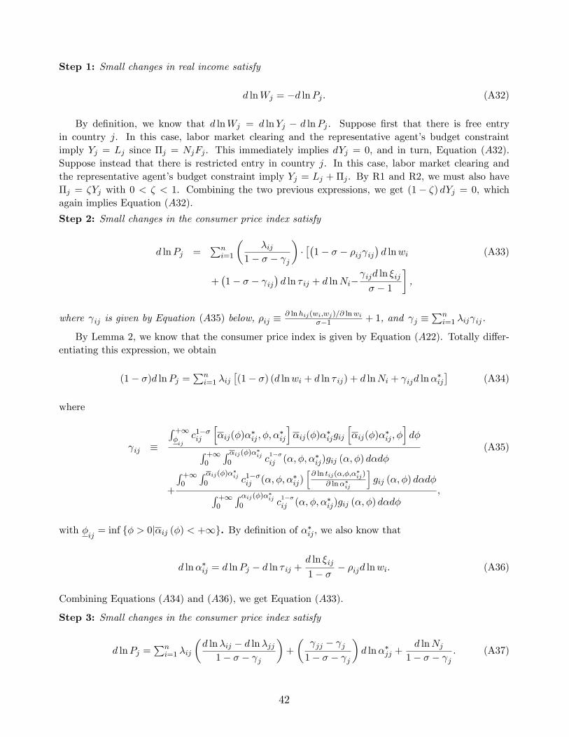
Step 1: Small changes in real income satisfy

d lnWj = �d lnPj . (A32)

By de�nition, we know that d lnWj = d lnYj � d lnPj . Suppose �rst that there is free entryin country j. In this case, labor market clearing and the representative agent�s budget constraintimply Yj = Lj since �j = NjFj . This immediately implies dYj = 0, and in turn, Equation (A32).Suppose instead that there is restricted entry in country j. In this case, labor market clearing andthe representative agent�s budget constraint imply Yj = Lj + �j . By R1 and R2, we must also have�j = �Yj with 0 < � < 1. Combining the two previous expressions, we get (1� �) dYj = 0, whichagain implies Equation (A32).

Step 2: Small changes in the consumer price index satisfy

d lnPj =Pni=1

��ij

1� � � j

����1� � � �ij ij

�d lnwi (A33)

+�1� � � ij

�d ln � ij + d lnNi�

ijd ln �ij� � 1

�,

where ij is given by Equation (A35) below, �ij �@ lnhij(wi;wj)=@ lnwi

��1 + 1, and j �Pni=1 �ij ij.

By Lemma 2, we know that the consumer price index is given by Equation (A22). Totally di¤er-entiating this expression, we obtain

(1� �)d lnPj =Pni=1 �ij

�(1� �) (d lnwi + d ln � ij) + d lnNi + ijd ln��ij

�(A34)

where

ij �

R +1�ij

c1��ij

h�ij(�)�

�ij ; �; �

�ij

i�ij(�)�

�ijgij

h�ij(�)�

�ij ; �

id�R +1

0

R �ij(�)��ij0 c

1��ij (�; �; ��ij)gij (�; �) d�d�

(A35)

+

R +10

R �ij(�)��ij0 c1��ij (�; �; ��ij)

h@ ln tij(�;�;�

�ij)

@ ln��ij

igij (�; �) d�d�R +1

0

R �ij(�)��ij0 c

1��ij (�; �; ��ij)gij (�; �) d�d�

,

with �ij= inf f� > 0j�ij (�) < +1g. By de�nition of ��ij , we also know that

d ln��ij = d lnPj � d ln � ij +d ln �ij1� � � �ijd lnwi. (A36)

Combining Equations (A34) and (A36), we get Equation (A33).

Step 3: Small changes in the consumer price index satisfy

d lnPj =Pni=1 �ij

�d ln�ij � d ln�jj1� � � j

�+

� jj � j1� � � j

�d ln��jj +

d lnNj1� � � j

. (A37)

42

By Lemma 2, we know that shares of expenditure are given by Equation (A23). Totally di¤erentiatingthis expression, we get

d ln�ij � d ln�jj = (1� �) (d lnwi + d ln � ij) + ijd ln��ij � jjd ln��jj + d lnNi � d lnNj .

By de�nition of ��ij , we also know that

d ln��ij = d ln��jj � �ijd lnwi � d ln � ij +

d ln �ij1� � .

The two previous expressions imply

d ln�ij � d ln�jj =�1� � � �ij ij

�d lnwi + (1� � � ij)d ln � ij (A38)

+ ijd ln �ij1� � +

� ij � jj

�d ln��jj + d lnNi � d lnNj .

Combining Step 2 and Equation (A38), we get Equation (A37).

Step 4: Small changes in the consumer price index satisfy

d lnPj = �d ln�jj"

+d lnNj"

. (A39)

Since d ln�ij � d ln�jj = d lnXij � d lnXjj , Equation (A38) implies, for any i; i0 6= j,

@ ln (Xij=Xjj)

@ ln � i0j= "ii

0j =

8<: 1� � � ij +� ij � jj

� �@ ln��jj@ ln � ij

�for i0 = i�

ij � jj� � @ ln��jj

@ ln � i0j

�for i0 6= i

.

Since@ ln��jj@ ln � i0j

=@ lnPj@ ln � i0j

> 0, the two previous equations together with R3 imply ij = 1� � � " for alli. Combining this observation with Step 3, we get

d lnPj =Pni=1 �ij

�d ln�ij � d ln�jj

"

�+d lnNj"

.

Equation (A39) derives from the previous expression and the fact thatPni=1 �ijd ln�ij = 0.

Step 5: Small changes in the number of goods that can be produced satisfy d lnNj = 0.

Suppose �rst that entry is restricted in country j. In this case, we immediately get d lnNj = 0.Now suppose that we have free entry instead. In this case, we know that �j = NjFj . Since �j = �Yjby R1 and R2, we therefore have d lnNj = d lnYj = 0, as demonstrated in Step 1.

Steps 1, 4 and 5 imply d lnWj = d ln�jj/ ". The rest of the proof is the same as under perfectcompetition. QED.

43

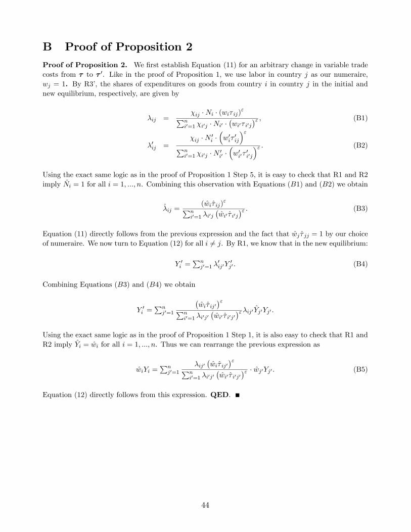
B Proof of Proposition 2Proof of Proposition 2. We �rst establish Equation (11) for an arbitrary change in variable tradecosts from � to � 0. Like in the proof of Proposition 1, we use labor in country j as our numeraire,wj = 1. By R3�, the shares of expenditures on goods from country i in country j in the initial andnew equilibrium, respectively, are given by

�ij =�ij �Ni � (wi� ij)"Pn

i0=1 �i0j �Ni0 ��wi0� i0j

�" , (B1)

�0ij =�ij �N 0

i ��w0i�

0ij

�"Pni0=1 �i0j �N 0

i0 ��w0i0�

0i0j

�" . (B2)

Using the exact same logic as in the proof of Proposition 1 Step 5, it is easy to check that R1 and R2imply Ni = 1 for all i = 1; :::; n. Combining this observation with Equations (B1) and (B2) we obtain

�ij =(wi� ij)

"Pni0=1 �i0j

�wi0 � i0j

�" . (B3)

Equation (11) directly follows from the previous expression and the fact that wj � jj = 1 by our choiceof numeraire. We now turn to Equation (12) for all i 6= j. By R1, we know that in the new equilibrium:

Y 0i =Pnj0=1 �

0ij0Y

0j0 . (B4)

Combining Equations (B3) and (B4) we obtain

Y 0i =Pnj0=1

�wi� ij0

�"Pni0=1 �i0j0

�wi0 � i0j0

�"�ij0 Yj0Yj0 .Using the exact same logic as in the proof of Proposition 1 Step 1, it is also easy to check that R1 andR2 imply Yi = wi for all i = 1; :::; n. Thus we can rearrange the previous expression as

wiYi =Pnj0=1

�ij0�wi� ij0

�"Pni0=1 �i0j0

�wi0 � i0j0

�" � wj0Yj0 . (B5)

Equation (12) directly follows from this expression. QED.

44