New Tools for Trapping and

Separation in Gas Chromatography and Dielectrophoresis

Improved Performance by Aid of Computer Simulation

Fredrik Aldaeus

Stockholm University

Doctoral thesis in analytical chemistry Stockholm University Department of Analytical Chemistry Stockholm, Sweden, 2007 Copyright © 2007 Fredrik Aldaeus All rights reserved for the main text of this thesis, including all pictures and figures. No part of this publication may be reproduced or transmitted in any form or by any means, without prior permission in writing from the copyright holder. The copyrights of the appended papers belong to the publishing houses of the journals concerned. ISBN 978-91-7155-526-7 Printed in Sweden by Intellecta Docusys, Stockholm 2007 Distributor: Stockholm University Library

Abstract Computer simulations can be useful aids for both developing new analytical methods and enhancing the performance of existing tech-niques. This thesis is based on studies in which computer simulations were key elements in the development of several new tools for use in gas chromatography and dielectrophoresis. In gas chromatography, gaseous analytes are separated by exploiting differences in their parti-tioning between different phases, and after their partitioning parame-ters have been determined the separations can be computationally predicted, and optimized, for a wide range of operating conditions. Similarly, in dielectrophoresis, particles with differing polarizability or size can be separated, and since particle trajectories within a sepa-ration device can be predicted using computations, the suitability of new designs, applications of forces and combinations of operational parameters can be assessed without necessarily making or empirically testing all of the variants.

Using two existing numerical methods combined with semi-empi-rical determinations of retention behavior, temperature-programmed gas chromatograms were predicted with less than one percent devia-tions from experimental data, and a new method for improving the capacity of a gas-trapping device was predicted and experimentally verified. In addition, two new concepts with potential capacity to en-hance dielectrophoretic separations were developed and tested in si-mulations. The first provides a promising way to improve the trap-ping of bacteria in media with elevated conductivity by using super-positioned electric fields, and the second a way to increase selectivity in the separation of bio-particles by using multiple dielectrophoretic cycles. The studies also introduced a more accurate method for deter-mining the conductivity of suspensions of bacteria, and a new compu-tational method for determining the dielectrophoretic behavior of par-ticles in concentrated suspensions.

The scientific studies are summarized and discussed in the main text of this thesis, and presented in detail in seven appended papers.

Keywords: gas chromatography, dielectrophoresis, computer simu-lation, finite element method, trapping, separation, lab-on-a-chip.

En sammanfattning på svenska finns som bilaga längre fram i avhandlingen!

Contents

Preface and acknowledgements 13

Introduction 15

Prediction of gas chromatograms 17 Separation optimization | Previous retention computations | Fundamental equations Parameter determination | Discretization methods

The iterative method for retention prediction 25 Customized software | Thermodynamic interpretation of retention data Predicted retention times

The finite element method for chromatogram prediction 29 Enhanced prediction possibilities | Predicted chromatograms | Discretization comparison

The enlarged tube method for increased trapping capacity 35 Breakthrough sampling | Ultra-thick film enrichment

Particle separation with dielectrophoresis 41 Forces acting on a polarizable particle | Dielectrophoretic motion Micro-scale separations of particles using electric forces

The superpositioned dielectrophoresis concept for improved trapping 47 Trapping in high conductivity media | Superpositioning of electric fields | Enhanced trapping

The multi-step dielectrophoresis concept for improved separation 51 Improving dielectrophoretic separations | Dielectrophoretic resolution and selectivity Enhanced separation power

Dielectrophoresis calculation methods 56 Model particles | Model chambers | Calculation procedure | Concentrated suspensions

The cross-flow filtration method for conductivity measurements 62 Gentle pre-handling of cells | Isoconductance point | Measurements of conductivity Conductivity of gently treated cells

Conclusions and future outlook 65

References 69

Appendix 1: Superpositioning of two alternating current electric fields in dielectrophoresis 83

Appendix 2: Complementary dielectrophoresis experiments 85 Preparation of beads and bacteria | Open dielectrophoresis device Positioning and separation of beads | Behavior of E. coli

Appendix 3: Populärvetenskaplig sammanfattning 91

List of papers

This thesis is based on the following seven papers, which are referred to in the text by the corresponding Roman numerals. Some unpublis-hed results are also presented.

I “Ultra thick film open tubular traps with an increased

inner diameter” Johan Pettersson, Fredrik Aldaeus, Adam Kloskowski, Johan Roeraade Journal of Chromatography A 1047 (2004) 93–99 doi:10.1016/j.chroma.2004.06.072 (Copyright © 2004 Elsevier. Reprinted with permission.)

II “Superpositioned dielectrophoresis for enhanced trapping

efficiency” Fredrik Aldaeus, Yuan Lin, Johan Roeraade, Gustav Amberg Electrophoresis 26 (2005) 4252–4259 doi:10.1002/elps.200500068 (Copyright © 2005 Wiley-VHC. Reprinted with permission.)

III “Multi-stepped dielectrophoresis for separation of particles”

Fredrik Aldaeus, Yuan Lin, Johan Roeraade, Gustav Amberg Journal of Chromatography A 1131 (2006) 261–266 doi:10.1016/j.chroma.2006.07.022 (Copyright © 2006 Elsevier. Reprinted with permission.)

IV “Simulation of dielectrophoretic motion of microparticles

using a molecular dynamics approach” Yuan Lin, Fredrik Aldaeus, Gustav Amberg, Johan Roeraade Proceedings of ICNMM 2006-96095 – 4th International Con-ference on Nanochannels, Microchannels and Minichannels, Limerick, Ireland, June 19–21, 2006 (Copyright © 2006 ASME. Reprinted with permission.)

V “Determination of conductivity of bacteria by using cross-flow filtration” LarsErik Johansson, Fredrik Aldaeus, Gunnar Jonsson, Sven Hamp, Johan Roeraade Biotechnology Letters 28 (2006) 601–603 doi:10.1007/s10529-006-0021-8 (Copyright © 2006 Springer. Reprinted with permission.)

VI “Prediction of retention times of polycyclic aromatic

hydrocarbons and n-alkanes in temperature programmed gas chromatography” Fredrik Aldaeus, Yasar Thewalim, Anders Colmsjö Analytical and Bioanalytical Chemistry 389 (2007) 941–950 doi:10.1007/s00216-007-1528-0 (Copyright © 2007 Springer. Reprinted with permission.)

VII “Prediction of temperature-programmed gas

chromatograms using the finite element method” Fredrik Aldaeus, Yasar Thewalim, Anders Colmsjö Journal of Chromatography A (2007), submitted

The contributions of the author of this thesis to these papers can be summarized as:

I Some of the writing, some of the calculations II, III Most of the writing, some of the calculations IV Minor part of the writing, some of the experiments V Some of the writing, some of the experiments and some of

the calculations VI Most of the writing, some of the calculations VII Most of the writing, most of the calculations

Related papers, not included in this thesis:

• “Retention time prediction of compounds in a test

mixture for apolar capillary columns according to Grob in temperature programmed gas chromatography” Yasar Thewalim, Fredrik Aldaeus, Anders Colmsjö Analytical and Bioanalytical Chemistry (2007), submitted

Some of the work underlying this thesis has also been presented at international conferences, as listed below:

• “A study of biological particles in a bio-MEMS device

using dielectrophoresis” Mats Jönsson, Fredrik Aldaeus, Lars-Erik Johansson, Ulf Lindberg, Johan Roeraade, Ylva Bäcklund, Sven Hamp, Gunnar Jonsson Proceedings of Micro Systems Workshop ’04, Ystad, Sweden, March 30–31, 2004 (paper and oral presentation)

• “Numerical predictions of continuous separations in a

microfluidic positive dielectophoresis system” Fredrik Aldaeus, Lin Yuan, Johan Roeraade, Gustav Amberg 4th Workshop on Nanochemistry and Nanobiotechnology, Saltsjöbaden, Sweden, August 25–27, 2004 (poster presentation)

• “Escherichia coli behavior in an open dielectrophoretic

microsystem” Fredrik Aldaeus, Lars-Erik Johansson, Mats Jönsson, Gunnar Jonsson, Ulf Lindberg, Johan Roeraade, Sven Hamp 4th Workshop on Nanochemistry and Nanobiotechnology, Saltsjöbaden, Sweden, August 25–27, 2004 (poster presentation)

• “Dielectrophoresis of living cells – new concepts and

challenges” Fredrik Aldaeus, Lin Yuan, Mats Jönsson, LarsErik Johans-son, Gunnar Jonsson, Johan Roeraade, Gustav Amberg 5th Workshop on Nanochemistry and Nanobiotechnology, Funchal, Madeira, Portugal, November 14–18, 2005 (oral presentation)

• “Simulation of Gas Chromatography”

Anders Colmsjö, Fredrik Aldaeus, Yasar Thewalim PittCon 2007, Chicago, IL, USA, February 25 – March 2, 2007 (oral presentation)

Papers II–V were previously included in a thesis for the degree Licen-tiate of Technology in Chemistry at the Royal Institute of Technology (KTH).

Abbreviations and notations

AC alternating current B. subtilis Bacillus subtilis DC direct current DEP dielectrophoresis E. coli Escherichia coli αDEP dielectrophoretic selectivity β phase ratio δ phase shift ∇ Del operator

2∇ Laplacian operator ΔH change in enthalpy ΔS change in entropy ω angular frequency DEPϑ dielectrophoretic mobility

φ electric potential κ~ effective polarizability D dispersion factor df thickness of the stationary phase film dM diameter of the mobile phase DM diffusion constant in the mobile phase DS diffusion constant in the stationary phase E electric field F force FDEP dielectrophoretic force h increased dispersion per column length unit KD distribution coefficient L length of column NDEP number of separation steps in multi-step dielectrophoresis p induced dipole moment q charge R molar gas constant R2 coefficient of determination

RDEP dielectrophoretic resolution t time T temperature uM velocity of the suspension medium / mobile phase unDEP velocity induced by negative dielectrophoresis upDEP velocity induced by positive dielectrophoresis utot total velocity V volume VB breakthrough volume VS volume of the stationary phase z position in column

13

Preface and acknowledgements

This thesis summarizes studies I have participated in at the Royal In-stitute of Technology (KTH) in Stockholm during 2002–2006, and at Stockholm University during 2006–2007. The thesis consists of a summary of six peer-reviewed papers (denoted Papers I–VI), and one that has been submitted to an international journal for peer-review (denoted Paper VII). The main scientific work is presented in these papers.

The aim of the thesis is to clarify my contributions to the included papers, to summarize the major scientific findings and highlight the common denominators in the included papers, and to comment on the work of other scientists in related areas.

The work presented in this thesis would not have been possible without the co-authors of the included papers and my other project co-workers. I would like to express my sincere gratitude to:

Anders Colmsjö, my supervisor at Stockholm University, for giv-ing me the opportunity to finish my postgraduate studies and for de-velopment of the software GC Interactive Simulation [Papers VI–VII].

Johan Roeraade, my supervisor at KTH, for introducing me to the world of science and to invaluable comments on my research and sci-entific writing [Papers I–V].

LarsErik Johansson at Mälardalen University, for the cell cultiva-tions, filtration equipment, and dielectrophoresis experiments [Paper V].

Mats Jönsson at Uppsala University, for manufacturing micro-chips for the dielectrophoresis experiments.

Yuan Lin at KTH, for the particle trace calculations [Papers II–IV].

Johan Pettersson Redeby at KTH, for gas chromatography experi-ments, for manufacturing the open tubular trap with increased inner diameter [Paper I], and for commenting on my thesis.

14

Yasar Thewalim at Stockholm University, for the gas chromatog-raphy experiments [Papers VI–VII].

Gustav Amberg at KTH, Ulf Lindberg at Uppsala University, Sven Hamp and Gunnar Jonsson at Mälardalen University, and Hywel Morgan and Nicolas G Green at the University of Southampton, for rewarding discussions about science in general and dielectrophoresis in particular.

Also thanks to Åsa Emmer, Bo Karlberg, Conny Östman and Gun-nar Thorsén for valuable comments on my thesis, to John Blackwell for proof-reading my thesis, and to all my past and present colleagues for creating a friendly and stimulating environment to work in.

I would also like to take the opportunity to thank my beloved wife Sara and my whole family for always believing in me. Without you, this would not have been possible!

The financial support from SSF (the Swedish Foundation for Stra-tegic Research) for the dielectrophoresis work is also gratefully ac-knowledged.

15

Introduction

The fundamental questions addressed by analytical chemists are: What types of substances are present in chemical samples, and in what quantities? If it is not possible to make a selective detection, the molecules or particles of interest (henceforward referred to as “ana-lytes”) must often be trapped and then somehow separated from other particles or molecules before those questions may be answered. For physical separation to occur, different analytes can be forced to move with different velocities. The magnitude of the difference in velocity required depends on the degree of dispersion that occurs during the movement. The key process of separation may thus be described us-ing two terms: a convective term describing the movement, and a diffusive term describing the dispersion.

This thesis discusses issues related to both the retention and sepa-ration of analytes in gas chromatography and dielectrophoresis, fo-cusing on new tools that have been developed during the course of the underlying studies to enhance these techniques. The new tools in-clude some that have been experimentally verified, and are hencefor-ward called “methods”, and others that have not yet been thoroughly tested in practice and hence are called “concepts”.

In the first part of this thesis, computer modeling of separations in gas chromatography is briefly discussed. Two methods to predict chromatographic data are presented. The first is based on an iterative method [Paper VI], and the second on the finite element method [Pa-per VII]. The thesis also describes a new sample trapping method that may be utilized when analyzing trace components in both gases and liquids [Paper I]. Both the precision of the predicted chromatograms and the new trapping approach have been experimentally evaluated using test mixtures and different columns.

Part two of this thesis describes two new concepts that may be used to increase the trapping and separation efficiency in dielectro-phoretic separations. In the first, two or more combined electric fields

16

are utilized [Paper II], while the second is based on a repetitive di-electrophoretic trap-and-release steps [Paper III]. The calculations de-monstrating these concepts were performed using Escherichia coli (E. coli) and polystyrene beads as model particles, because of the impor-tance of these micro-organisms and particles in biotechnology [1]. The calculations also include some initial predictions regarding the behavior of concentrated particle suspensions [Paper IV].

Tentative experimental dielectrophoresis work has been performed using the same materials as in Papers II and III (i.e. E. coli and po-lystyrene beads) [Appendix 2]. The experimental work also included tests of a new, more reliable method for measuring the conductivity of living cells [Paper V].

17

Prediction of gas chromatograms

Separation optimization

Gas chromatography can be used to separate the components of any mixture that are sufficiently volatile and thermally stable. Although the basic principles have been known for decades, a tremendous amount of research is still in progress to enhance the possible applica-tions of the technique [2].

One way to improve separations by gas chromatography is to gain more knowledge about the systems through computer simulations. Experimental data can be compared to calculated results with an ap-propriate model, and this may provide more knowledge about the im-pact of physical parameters on retention and separation. Furthermore, deviations between predicted and experimentally acquired results can provide indications of second and third order perturbations, such as concentration dependence, adsorption and nonlinear behavior.

Nevertheless, the most important reason for trying to predict chro-matographic behavior is that computation may dramatically reduce the number of required preliminary experimental runs needed to opti-mize a complex separation.

Optimizing the separation of a mixture of analytes in gas chroma-tography involves a number of steps [3], including: 1) selection of an appropriate column, which heavily depends on the size and polarity of the target analytes; 2) high temperature isothermal runs, to ensure that the heaviest analytes are eluted; 3) low temperature isothermal runs, to ensure that the lightest analytes are separated; 4) identifica-tion of peaks; 5) temperature and/or pressure programming, if it is not possible to separate all the analytes at a single temperature; 6) re-identification of peaks, since the elution order (especially of polar analytes) may vary depending on the temperature range and gradient.

18

If some analytes still are still not separated after these steps, a new column must be chosen, and the steps must be repeated.

In contrast to time-consuming optimization by performing several experiments, the results of varying running conditions may be quickly predicted using computations. If retention data for different analytes in different columns are available (from previous isothermal experi-ments, for instance) it will be possible to run the whole temperature programming procedure on a computer, thereby dramatically reduc-ing the time needed to optimize a separation.

Previous retention computations

Several authors have made important contributions to simulations of gas chromatographic analyses. As early as the 1960s, Habgood & Harris [4] used isothermal retention data to predict elusion tempera-tures in temperature-programmed experiments. A major step forward came in the late 1980s when Dose [5, 6] proposed that thermody-namic parameters obtained from isothermal measurements could be used as retention indices for temperature-programmed experiments. By integrating zone velocities, he was able to predict retention times with an accuracy of 1% and peak widths with an accuracy of 15%. At the same time, Arkporhonor et al. [7–10] introduced a procedure for determining retention times that included the determination of upper integral limits, using numerical integration and a root-trapping ap-proach.

Since then, Bautz, Dolan and Snyder [11–13] have used an empiri-cal two-parameter model based on a simplified linear-elusion-strength approximation to predict the retention times of different polar and non-polar test-substances. The differences between the predicted and experimental results are typically a few percent. Later, Snijders et al. [14, 15] introduced a method allowing retention parameters to be de-termined without solving any integrals, using retention indices deter-mined by other authors. This numerical approach modeled the chro-matographic processes of the analytes in very small, regular time seg-ments. The iterative method described later in this thesis is mainly based on this approach.

Important work was undertaken by Vezzani, Castello and Moretti [16–19] when they tested several methods for predicting retention parameters and were able to determine retention times for a number of different analytes with errors of only circa 1%. They later used thermodynamic retention data to classify different columns and sta-

19

tionary phases [20]. They have also showed that the main source of errors when predicting retention times is associated with the instru-mentation and not the theoretical approach. The most important sour-ce of errors is the difference between the temperature programs used in the calculations and the actual temperatures in the gas chromato-graph oven [21]. Recently, they have evaluated peak shapes [22] and predicted separation numbers [3].

Several important theoretical and practical aspects of temperature-programmed gas chromatography that should be considered when calculating chromatograms have been discussed by Gonzalez [23–34], Wu [35] and Castells [36, 37].

By using a numerical approach based on the Euler approximation, Chen et al. [38–40] have predicted retention times in combined tem-perature and pressure programmed gas chromatography. Recently, Dorman et al. [41] have used computer modeling of gas chromatog-raphy to design optimized columns to address specific separation problems. Also notable is the work of Zhang and co-workers [42], who predicted retention times of volatile compounds using a heuristic method and support vector machine based on descriptors calculated from molecular structures alone.

Fundamental equations

In order to calculate chromatographic parameters of any kind, a gov-erning equation must be constructed. The solution of this equation should give the concentration c of an analyte at time t for all positions in the column. The equation must include a convective term that de-scribes the movement of the analyte packet (a packet of analyte gas is subsequently referred to as a “peak”), and a diffusive term accounting for the dispersion during the movement of the peak in the column. Since the analyte is distributed between a mobile gas phase and a re-taining stationary phase, the time-scale must be adjusted to account for the fact that only a fraction of the analyte is moving at any given time.

Open tubular gas chromatography can be fundamentally viewed as a three-dimensional problem with axial symmetry. However, it is of-ten convenient to reduce the calculations to a one-dimensional prob-lem in the column axis direction (subsequently referred to as the z-axis). To meet these requirements, a transient convection-diffusion equation may be written as [43–49]

20

DM1 K c c cu D

β t z z z⎛ ⎞ ∂ ∂ ∂ ∂⎛ ⎞+ = − +⎜ ⎟ ⎜ ⎟∂ ∂ ∂ ∂⎝ ⎠⎝ ⎠

(1)

where KD is the distribution coefficient of the analyte between the mobile and stationary phases, β is the ratio between the volumes of the stationary and mobile phases, uM is the average linear velocity (in the z-direction) of the mobile phase, and D is a dispersion factor de-noting the change in variance (in the z-direction) per unit time of a normalized peak.

The dispersion term consists of contributions due to both static dif-fusion (which occurs whether the mobile phase is moving or not), and velocity-dependent dynamic diffusion (due to fluctuations in occu-pancy of the various portions of the cross-section and the stationary phase). The term may be expressed as

M2hD u= (2)

where h denotes the increased dispersion per unit column length dur-ing the movement of the peak along the column axis (i.e. the factor often referred to in the literature as the “height equivalent of a theo-retical plate” [50]). An expression for this axial dispersion, including both the static and dynamic diffusion in cylindrical gas chromatogra-phy (based on the original equation by Golay [43]) is

( ) ( )

2 2 2 2D D M D f

M M M2 2M M sD D

6 11 21296 3

β K β K d K β dh D u uu D Dβ K β K

+ += + +

+ +

(3) where DM and DS are the diffusion coefficients of the analyte in the mobile and stationary phases, respectively, dM is the diameter of the mobile phase, and df is the thickness of the stationary phase film. Note that in Equation 3 the original cylindrical dispersion problem is reduced to a one-dimensional case. To deduce the equation, a number of assumptions have to be made [43, 51]: • The stationary phase consists of a uniform retentive coating on

the inner wall of the column. • The mobile phase contains KD/β times as many analyte molecules

at equilibrium as the stationary phase. • The variation of sample density within any thin section of the co-

lumn is negligibly small when compared to the density itself

21

• The diffusion within the stationary phase is instantaneous if the analyte concentration in the stationary phase is zero. If the analyte concentration is not zero in the stationary phase, the diffusion time is finite.

• The mobile phase has a Poiseuille (i.e. parabolic) flow profile, and the axial velocity of the mobile phase at the boundary be-tween the mobile and the stationary phase is zero.

In a given column, the volume phase ratio, the mobile phase dia-meter and the stationary phase thickness can all be regarded as con-stant. The actual values of these parameters are often specified by the manufacturer. However, in order to solve the equation for chromato-graphic motion, the distribution coefficient, the mobile phase veloc-ity, and the diffusion coefficients must be determined. These parame-ters depend on the temperature, and their values at an arbitrary tem-perature can be determined by performing isothermal experiments and then fitting the results to an appropriate model.

In cases of retention due to adsorption, the factor in front of the concentration time derivative on the left-hand side of Equation 1 must be modified to account for concentration dependence (the exact modi-fication will depend on the kind of adsorption isotherm that may be assumed) [52].

Parameter determination

The first properties to determine are often the retention characteris-tics. If the column phase ratio is known, the retention of an analyte will depend on its distribution coefficient. Tentative calculations per-formed in our laboratory have shown that the easiest way to deter-mine this coefficient is to make a model (in our case, a partial least-squares model) based on boiling points and molecular weights. This works fairly well for homolog series such as n-alkanes, but for slight-ly more complex molecules such as polycyclic aromatic hydrocar-bons or the polar substances in a “Grob calibration mixture”, the boil-ing point method for determining the retention parameters at a speci-fied temperature is not sufficient. A better strategy to determine the retention at different temperatures is often to use either an empirical or a semi-empirical approach [33]. In a purely empirical approach, re-tention data from isothermal experiments are either simply interpola-ted to obtain approximations of retention at different temperatures, or fitted to an arbitrary function such as a polynomial with a suitable number of parameters. In a semi-empirical approach, the data are

22

fitted to a model based on information acquired from macroscopic thermodynamic observations regarding the temperature dependence of the analytes’ distribution between two phases [6, 20]. A semi-em-pirical approach involving the determination of two or three thermo-dynamic parameters was applied in Papers VI–VII.

Note that a distribution coefficient as a function of temperature is only valid for one specific analyte and stationary phase combination. Hence, it is not necessarily possible to use a set of data obtained with one stationary phase to predict retention parameters with another sta-tionary phase. However, the distribution coefficients do not depend on the size of the column. Hence, retention parameters can be predict-ted in another column, provided that the stationary phase is of the same type.

In addition to the distribution coefficients, the linear velocity of the mobile phase must also be determined at different positions in the co-lumn. This depends on the column dimensions and the pressure drop over the column [14, 15, 28]. If the column dimensions, the actual temperature, and the mobile phase gas, are known, the inlet pressure may be determined implicitly by experimentally determining the gas hold-up time (i.e. the elution time for an analyte without retention) [28]. When the inlet and outlet pressures have been calculated, the pressure at an arbitrary position in the column may be determined. Once this is done, the mobile phase velocity may be determined as a function of column temperature and position in the column using Na-vier-Stokes equations [28].

If accurate determinations of the retention characteristics and mo-bile phase velocity are carried out, the retention times and hence also the elution order of analytes can be determined. However, optimizing resolution also requires accurate prediction of dispersion, which is of-ten more difficult and requires sufficiently accurate measures of dif-fusion constants. The diffusion constants of the analytes may be de-termined using the expanded method presented by Fuller et al. [53], which include calculating the atomic and structural diffusion volumes and the molar weights of the analytes and the mobile phase gas. Fol-lowing determination of the diffusion constants in the gas phase, the diffusion constants in the stationary phase are often approximated as being four orders of magnitude lower those in the gas phase [53]. This gives reasonable accuracy for most calculations.

23

Discretization methods

In order to solve a chromatography equation, the column and the timescale must be divided into small segments of finite size. This allows the partial differentials in the original equation (i.e. Equation 1) to be replaced by approximate differences. This is called discreti-zation of the problem.

A commonly used discretization method is the finite difference method [54], in which the length scale of the column as well as the time scale for the separation is divided into small segments of equal or unequal size. The goal is then to calculate the concentration of each analyte in all the column segments for all time segments. This is done by replacing all differentials in the equation with finite differ-entces. The replacement may be done using explicit, implicit or com-bined algorithms. This generates a system of linear equations that may be solved using standard methods.

The finite element method [55, 56] (often referred to as finite ele-ment analysis) is an approach wherein the solution to the equation, rather than the differential equation itself, is approximated. This is done by assuming that the solution can be approximated by a linear combination of an appropriate basic function. This usually makes the computation more time-consuming, but the results are often more accurate. However, the main advantage of the method is that it is straightforward to use for complex geometries, which makes it very useful for calculations in fields such as structural mechanics and fluid dynamics [57–60]. In gas chromatography, the geometry is very sim-ple, but the ease of its implementation (even if, for instance, adsorp-tion isotherms and other irregularities are added to the equation) and wide variety of commercially available software make it attractive even for separation calculations. In Paper VII, the finite element method is used to calculate the concentrations of the analytes in the different segments of the column. The method is also used in Papers II–IV, but in these cases to determine an electric field and a fluid velocity field.

Another method that may be used for chromatography calculations is an iterative approach in which the peak positions and widths are calculated separately [14, 15]. Here, only the time is divided into small finite units. The velocities of all analyte peaks are determined at a starting position. Once determined, the new positions of the peaks may be determined at the next time-step. Velocities at the new posi-tions are calculated, followed by a new iteration, and so on. The pro-cedure is repeated until the positions of the peaks exceed the column

24

length. For all time-steps, the peak dispersions within them are calcu-lated. When a peak exceeds the length of the column, the dispersions for all time-steps are summarized to obtain the total dispersion. This drastically reduces the computation time since computation of con-centration of all analytes at all positions for all time-steps is avoided. If the dispersion is purely Gaussian (with no tailing or leading of peaks), and a large numbers of analytes are to be predicted, this may be a good alternative to the finite difference or finite element meth-ods.

25

The iterative method for retention prediction

Customized software

Several software packages for chromatographic calculations are avai-lable on the market, for instance EZ-GC (Restek Corporation, Belle-fonte, PA, USA) [60], DryLab GC (LC Resources, Inc., USA) [12, 61], GC-SOSTM (ChemSW, USA), and ACD/GC (Advanced Chemis-try Development, Inc., USA). Provided that the data input for these programs are sufficiently fine, they are all able to predict retention times with a precision of a few percent or better.

In the study presented in Paper VI, software called GC Interactive Simulation was used. This package was originally designed as a tool for teaching chromatography at Stockholm University, but it can also be used for research purposes. One advantage of using software de-signed in-house is that it can easily be modified to account for differ-ent needs. It is, for instance, easy to modify the method used for the retention calculations.

In Paper VI, a two-parameter semi-empirical model of the reten-tion was used. Using least-squares fitting, the partition coefficients for each analyte-column pair were determined as a function of tem-perature using the equation

D1ln ( ) S HK T

R R TΔ −Δ

= + ⋅ (4)

where ΔS and ΔH are the changes in entropy and enthalpy, respec-tively, for an analyte when it is transferred from the mobile phase to the stationary phase, and R is the molar gas constant. Note that when using this equation, the entropy and enthalpy are assumed to be inde-pendent of temperature [5]. In practice, they do slightly depend on

26

temperature, but the obtained results may be considered an average value in the temperature interval wherein the isothermal runs were performed.

When the partition functions had been determined, the parameter values were exported to the software, together with data regarding the column, running conditions, etc.

The GC Interactive Simulation software is based on the iterative method briefly described above (under Discretization methods). Since merely the convection part of Equation 1 (i.e. the first term) is con-sidered when only the analyte peak positions are to be determined, the equation may be simplified and discretized into finite time-steps, giving the equation

DM

1 11 K uβ t z

⎛ ⎞+ = −⎜ ⎟ Δ Δ⎝ ⎠

(5)

If the position zi of a peak in one time-step i is known, its position in the next step (i.e. at time Δt later) can then be determined from Equation 5, re-written as

M,ii+1 i

D, i1

uz z tK= + ⋅Δ

+β

(6)

The retention time for an analyte is given by interpolation between the peak positions at the last time step before the peak reaches the end of the column end, and the first time step at which the peak has passed beyond the end of the column.

Thermodynamic interpretation of retention data

Isothermal retention data in 10 °C increments were acquired for two analyte mixtures (an n-alkane mixture [62] and a mixture of policy-clic aromatic hydrocarbons [63, 64]) in three columns with different polarities (DB-1, DB-5 and DB-17 (Agilent Technologies)). Partition coefficients were calculated for all analytes in all columns at all tem-peratures. The results were fitted to Equation 4, thereby providing va-lues of ΔS and ΔH (reported in Paper VI).

It is possible to use the semi-empirical values of the thermodyna-mic properties for more than just determination of the partition coef-ficients at different temperatures. Interpretation of the thermodynamic properties may also provide insights regarding the retention mecha-

27

nisms. If the retention is dominated by the entropy variations between the mobile and stationary phases, the separation is said to be entropy-driven. This is normally the case in, for instance, size exclusion chro-matography, where the analytes do not interact with the stationary phase per se, but rather are retained by the stationary phase due to the loss in the molecules’ translational, rotational and vibrational degrees of freedom. In partition chromatography (as in standard open tubular chromatography), the separation is normally enthalpy-driven, which is equivalent to saying that the dissolution energies of the analyte in the mobile phase and stationary phases differ.

If the retention time changes for an analyte as the polarity of the stationary phase changes, this may be due to variation in either the entropy or the enthalpy (or a combination thereof). Since the entropy and enthalpy values could be considered constant in the mobile phase, any change in ΔS or ΔH for an analyte when one column is replaced by another must be due to a change in the analyte’s entropy or enthal-py in the stationary phase.

In the study presented in Paper VI, the solvation entropies of the measured n-alkanes were similar in the non-polar DB-1 column and the slightly polar DB-5 column. In the more polar DB-17 column, the entropies decreased. The enthalpies of the n-alkanes were approxi-mately equal in all three columns. The differences in retention times of the n-alkanes were therefore likely to be due to variations in the degrees of freedom of the analytes in the different columns’ station-ary phases. However, the value of ΔH was much larger than ΔS, and the separation was hence likely to be enthalpy-driven. For the same reason, the retention of polycyclic aromatic hydrocarbons could be assumed to be enthalpy-driven. Furthermore, for the polycyclic aro-matic hydrocarbons, both the entropy and enthalpy decreased as the polarity of the stationary phase increased. Since a decrease in the en-tropy should result in a decreased retention time, but the retention times increased, the enthalpy was the dominating factor.

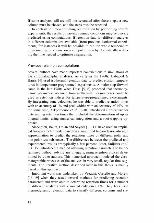
Predicted retention times

Using the isothermally obtained partition coefficients, temperature-programmed retention times were calculated. Experimental chroma-tograms using the same running conditions were then measured, and the results were compared. Examples are presented in Figure 1. For the n-alkanes and the polycyclic aromatic hydrocarbons, the different-ces between the predicted and experimentally determined retention

28

times were in the order of 1%. This may be considered adequate for a temperature-programmed run, since the deviations are close to the ex-perimental precision. For instance, in many commercially available column ovens, the temperature is controlled with an accuracy of ap-proximately ±1% [21]. This error in temperature is sufficient to cause errors in retention times close to the differences between the predict-ted and experimental results. To further reduce the discrepancies be-tween the predicted and experimental results, the experimental run-ning conditions would have to be more tightly controlled.

a)

b)

Figure 1. Comparisons between predicted and experimentally obtained chromatograms for a mixture of 16 polycyclic aromatic hydrocarbons. The predicted chromatograms are displayed below the experimental. (a) Parts of the chromatogram wherein all the analytes are eluted. (b) A close-up displaying peaks of three of the analytes. The figure shows (inter alia) that the predicted retention times are slightly shorter than the ex-perimental times.

29

The finite element method for chromatogram prediction

Enhanced prediction possibilities

The retention times predicted using the iterative method described in Paper VI were considered sufficiently accurate for most purposes. It is however of great interest to investigate whether a more detailed model could provide even more accurate predictions. Two approaches for making better predictions are 1) to use a more detailed function for the temperature dependence of the partition coefficients, and 2) to use a more sophisticated discretization method. In the study presented in Paper VII, both of these approaches were employed.

For the partition predictions, the entropy differences and enthalpy differences associated with movement of the analytes between the mobile and stationary phases (ΔS and ΔH) were considered in con-junction with the temperature, since they both depend on the differ-ences in isobaric heat capacity, ΔCp, associated with these move-ments. Therefore, an arbitrary reference temperature is chosen (for instance 0 °C, or a temperature within the range of the temperature program). ΔS and ΔH values at this reference temperature, and the isobaric heat capacity difference, can then be calculated by fitting ex-perimentally acquired data regarding partitioning at different tempe-ratures to the three-parameter semi-empirical equation [23, 28, 33].

ref refD

p ref ref

( ) ( ) 1ln ( )

1 ln

S T H TK TR R T

C T TR T T

Δ −Δ= + ⋅

−Δ ⎛ ⎞⎛ ⎞+ ⋅ − −⎜ ⎟⎜ ⎟⎝ ⎠⎝ ⎠

(7)

30

The column axis is divided into small mesh elements, and the sub-sequent discretization may be performed by approximating the solu-tion with a combination of finite quadratic elements [55]. This makes it possible to solve the full transient convection-diffusion equation (i.e. Equation 1) by reducing the partial differential equation to a sys-tem of ordinary differential equations. This will provide detailed in-formation on both retention times and peak widths, since the concen-tration of all analytes are given in all mesh elements for all time-steps. The retention time of an analyte is given by the time at which the concentration of that analyte reaches its maximum value at the end of the column.

Predicted chromatograms

As in the study presented in Paper VI, isothermal retention data in 10 °C increments were acquired. However, in this study using the finite element method (software Comsol Multiphysics (Comsol AB, Swe-den)) and the three-parameter equation, a test mixture of 2,6-dime-thylphenol, dodecane and methyl decanoate was used. Retention data were collected for four columns with different polarities (DB-1, DB-5, DB-17 and DB-23 (Agilent Technologies)). Using Equation 7 to determine the retention coefficients at different temperature, the chro-matograms obtained using different temperature programs (with 4 °C/min and 8 °C/min temperature gradients) were predicted for all four columns. Two examples are depicted in Figure 2. The different-ces in retention times in the printed chromatograms are almost invisi-ble to the naked eye. In the best predicted case, the discrepancy in re-tention time is less than 1 s, which corresponds to an average relative error of 0.05%. Even in the least well predicted case, the time differ-ence is only around 2 s.

Figure 2 also highlights the fact that the retention order changes as the polarity of the stationary phase changes. The ability of the method to accurately predict the changing positions is more pronounced in Fi-gure 3. This figure depicts all predicted chromatograms obtained for all columns and both temperature programs. The arrows indicate how the elution times are altered.

31

a)

Time [minutes]

b)

Time [minutes]

Figure 2. Comparison of two predicted and two experimentally deter-mined chromatograms. The DB-1 column with a 4 °C/min gradient in the temperature program gave the best prediction (a), whereas the DB-23 column with an 8 °C/min gradient gave the least good prediction (b).

32

Time [minutes] Time [minutes]

Figure 3. Predicted chromatograms resulting from separations of a mix-ture containing 2,6-dimethylphenol, dodecane and methyl decanoate us-ing four different columns (DB-1, DB-5, DB-17, DB-23) and two different temperature gradients (4 °C/min and 8 °C/min).

33

Discretization comparison

Illustrative comparisons of some of the retention times obtained with the iterative method, the finite element method and empirical deter-minations are presented in Table 1. For this evaluation, the same three-parameter model of the temperature dependence of the distribu-tion coefficients was used in the iterative method to the one used in the finite element-based study. For both temperature gradients, the results of the finite element method were substantially better than those obtained with the iterative method. The finite elements method can also provide satisfactory predictions of peak widths. Even though no extra-column effects were considered, the predicted peak widths were only approximately 10% lower than the experimentally determi-ned widths, while there were 40% discrepancies between the results obtained with the iterative method and the experimental data.

The main benefit of using the iterative method instead of the finite element method is that it is easier to use, and that the calculations take seconds instead of minutes to perform. Hence, the relative merits of high quality results and rapid computation times must be weighed for specific applications of these measures.

Table 1. Comparison between empirically determined and predictions of retention times (for three test substances in a DB-1 column) obtained using Comsol Multiphysics (finite element method) and GC Interactive Simula-tion (iterative method) software. In both cases three-parameter semi-empirical estimations of the retention times were used. (a) Predictions with a 4 °C/min gradient. (b) Predictions with an 8 °C/min gradient.

a) 4 °C/min Experimental Finite element method Iterative method*

Retention time [min]

Retention time [min]

Relative difference

Retention time [min]

Relative difference

2,6-dimethylphenol 11.85 11.86 –0.11% 11.81 0.37%

Dodecane 16.47 16.48 –0.04% 16.42 0.35%

Methyl decanoate 20.25 20.25 0.00% 20.18 0.34%

b) 8 °C/min Experimental Finite element method Iterative method*

Retention time [min]

Retention time [min]

Relative difference

Retention time [min]

Relative difference

2,6-dimethylphenol 9.22 9.20 0.17% 9.17 0.56%

Dodecane 11.72 11.69 0.20% 11.66 0.52%

Methyl decanoate 13.74 13.71 0.19% 13.67 0.54%

*) Unpublished results

34

35

The enlarged tube method for increased trapping capacity

Breakthrough sampling

Before analytes of interest in a sample can be analyzed by gas chro-matography, it is often necessary to trap and concentrate them. Sev-eral gas enrichment methods based on adsorption are available, such as solid phase micro-extraction [65], and devices such as large size sorptive probes [66]. A common feature of these methods and devices is that they rely on the establishment of partial or complete equilib-rium. If the equilibrium values are unknown, subsequent quantifica-tion of the analytes may be difficult. However, if the analytes are trapped in an open tubular column trap with a sorptive film, the sam-ple may be driven through the column until a certain amount of ana-lyte exits from the end of the trap. Another advantageous feature of using sorption rather than adsorption is that since the interaction be-tween the analyte and the trapping phase is weaker, high temperatures may not be needed in the subsequent desorption. This is especially advantageous if the analytes are unstable at elevated temperatures [67–69].

The gas volume that has passed the front end of a column before the concentration of the analyte in the effluent gas reaches a determi-ned percentage of the concentration in the inlet gas is often defined as the breakthrough volume VB [70]. The breakthrough volume may be used as a quantitative measure of the trapping capacity, and may be determined from

( )B S D ( , , )V V β K f L h b= ⋅ + ⋅ (8)

where VS is the volume of the stationary sorptive trapping phase and f is a trapping function of the column length (L), the increased disper-

36

sion per unit column length (h), and the tolerable level of break-through (b). If a breakthrough of 5% is accepted, the trapping func-tion f(L, h, b) in Equation 8 can be written [70] as

2

2

1( , , 0.05)5.360 4.6030.9025

f L h bh h

L L

= =

+ +

(9)

Open tubular traps are often similar to gas chromatography col-umns with respect to the materials chosen. However, in contrast to a separation in gas chromatography, the linear velocity of the mobile phase (i.e. of the sample matrix) is not as relevant in practice as the sampling flow rate. To determine the dispersion, it is hence more use-ful to rewrite Equation 3 in terms of flow rate instead of velocity:

( )

( )( )

2 2 2M M D D

2MD

2

D

2SD

6 111 14 24

2 1 13

πd D β K β Kh FF πDβ K

β β KF

πDβ K

+ += +

+

+ ++

+

(10)

where F is the average volume flow rate of the mobile phase. If the analyte is volatile (and hence has a low distribution coeffi-

cient) or very low detection limits are required, the trapping may be difficult since the breakthrough volume must be high to ensure that a sufficient amount of analyte is trapped. As indicated by Equation 8, the breakthrough volume largely depends on the volume of the sta-tionary phase. Thus, one strategy would be to simply increase the length of the tube. However, that approach has the disadvantage that it is limited by the accompanying increase in pressure drop. Another strategy to increase the trapping capacity is to use a large number of short narrow tubes [71, 72]. However, the retention power for highly volatile analytes in such tubes is often unsatisfactory. A more effi-cient and technically more favorable [71, 73, 74] method is to in-crease the volume of the stationary phase by making the sorptive film thicker. Provided that the flow rate is sufficiently high to assume neg-ligible static longitudinal diffusion (which applies in most experimen-tal cases), the first term on the right-hand side of Equation 10 equals zero, and the dispersion will hence not depend on the diameter of the column, provided that the phase ratio is kept constant. Consequently, it should be possible to increase the trapping capacity by simultane-ously increasing the film thickness and the column diameter.

37

In Figure 4, the calculated breakthrough volumes for hexane in three open tubular traps are depicted [Paper I]. The traps all have the same phase ratio, but different inner diameters (and, hence, different amounts of stationary phase). From this figure, it can be seen that the trap with the largest inner diameter also has the highest breakthrough volume. Even if the flow rate is very large, a high breakthrough vol-ume is achieved. The figure also shows that the trapping volume is only significantly reduced by longitudinal diffusion for the trap with the largest inner diameter.

Figure 4. Calculated breakthrough volumes (for a tolerable level of 5%) for hexane, in traps consisting of a polydimethylsiloxane stationary sorp-tive trapping phase in columns with three different diameters, as a func-tion of average flow rate. Hexane is assumed to have a distribution coef-ficient of KD = 200 at room temperature. All traps are assumed to have a phase ratio of unity (i.e. β = 1), and inner diameters of 0.7 mm (solid line), 1.5 mm (dotted line) and 4.5 mm (dashed line). The corresponding sorbent volumes are 0.385, 1.77 and 15.9 ml, respectively.

38

Ultra-thick film enrichment

The theoretical conclusions regarding the effects of increased film thickness and diameter were tested experimentally in a series of elu-tion analyses of hexane with three different traps [Paper I], subse-quently called Trap #1, Trap #2 and Trap #3 (see Paper 1 for detailed information regarding the traps’ length, phase ratio, etc.). Trap #1 had a phase ratio of circa 1.3, whereas the other two traps (#2 and #3) both had a phase ratio of circa 1.1.

In all traps, the gas flow rate through the column was varied, and the dispersion was measured. The dispersions, expressed as H-values, are given in Figure 5. Even though Trap #3 had an inner diameter al-most twice as large as that of Trap #2, the dispersions were almost identical at the same flow rates. Trap #1 and Trap #2 had identical inner diameters, but the h-values were lower in Trap #1 due to its higher phase ratio, and probably partly due to its smoother surface.

When the values of the trapping function in Equation 8 had been determined, the breakthrough volumes of the three traps were calcu-lated (Figure 6). The predicted and experimental results show good agreement, and for the smooth Trap #1, the differences were tiny. The experimental values for Trap #3 (acquired with both frontal and elu-tion analysis [Paper I]) were less reproducible, but agreed on average with the predicted values.

Despite Trap #3 being shorter than Trap #2, its breakthrough vol-ume was more than twice as large. Trap #1 has a lower breakthrough volume since it is only half as long as Trap #3. The experiments con-firm that the model for trapping in open tubes with thick films is va-lid. Thus, it may also be valid to speculate about other implications of the concept. For instance, if a trap with an even larger inner diameter was used, the pressure drop would be low enough to take samples without using pumps. This may be useful for sampling in open air with only the wind as driving force, or for sampling trace volatile analytes in alveolar air using only “lung power”. The limit for the dia-meter of traps for such applications would probably be set by practi-cal considerations and the fact that a high amount of sorption phase would result in a large desorption volume and high levels of back-ground noise due to sorbent degradation and the sorption of non-tar-get analytes.

39

Figure 5. Experimentally acquired h-values as a function of average flow rate for three traps. The traps have equivalent phase ratios, but the sta-tionary phase volume vary (due to differences in the inner diameter and length of the columns [Paper I]). The experimental values are depicted as circles (Trap #1), crosses (Trap #2) and squares (Trap #3).

Figure 6. Predicted and experimental values for the breakthrough volumes (for a tolerable level of 5%) of hexane in the three traps. The predicted va-lues are plotted as curves, whereas the experimental values are depicted as circles (Trap #1), crosses (Trap #2), squares (Trap #3, frontal analysis) and diamonds (Trap #3, elusion analysis).

40

41

Particle separation with dielectrophoresis

Forces acting on a polarizable particle

If a charged particle is placed in an electric field, it will be affected by a force proportional to the electric charge in the direction of the field (Figure 7a). Thus, if the charge is q and the field is E, the force is

F =qE (11) If a particle with no net charge, but with the ability to be polarized

is placed in an electric field between two electrodes, the charges in the particle are displaced in the direction towards the electrode with the opposite sign. Thus, the particle will be affected by a force in both directions. Since these two forces are equal in magnitude but have op-posite directions, there will be no net movement (Figure 7b). How-ever, if the particle is placed in an electric field that is not uniform, the particle will be affected by a net force in the direction towards the higher field strength (Figure 7c). This phenomenon is called dielec-trophoresis [75]. The net dielectrophoretic force FDEP is proportional to the polarizability of the particle and the inhomogeneity of the elec-tric field.

( )EpF ∇⋅=DEP (12)

where p is the induced dipole moment, E is the electric field, and ∇ is the Del operator (gradient). In two Cartesian dimensions, the Del operator is defined as

Iñ ó

⎛ ⎞∂ ∂∇ = ⎜ ⎟∂ ∂⎝ ⎠

(13)

42

Particles in chemical applications are often suspended in a liquid medium. If the medium is polarizable and the force on the medium is stronger than the force acting on the particle, the particle will be dis-placed in the direction towards the lower field strength. This motion is called negative dielectrophoresis. Positive dielectrophoresis will occur when the force on the particle is stronger than the force on the medium, and the particle is moving in the direction towards higher field strength.

The induced dipole moment depends on the effective polarizability (κ~) and the volume (V) of the particle, and the electric field:

p = κ~VE (14) The effective polarizability (κ~) can be calculated from the shape

of the particle and the dielectric properties (the conductivity and per-mittivity) of the particle and the surrounding medium. The larger the volume of the particle, the larger the dipole moment will become since the charges may be more separated, whereas the magnitude of the electric field determines how much the charges are displaced. If Equations 12 and 14 are combined, it can be seen that the dielectric force is proportional to the square of the electric field:

2DEP 2

~EF ∇=

Vκ (15)

Since 22 EE −= , the sign of the field has no influence. Thus, if the direction of the field is reversed, the movement will still be in the same direction. Consequently it is possible to use an alternating cur-rent (AC) electric field instead of a direct current (DC) electric field. A benefit of this is that the effective polarizability is dependent on the frequency of the applied field. For low frequencies, the effective po-larizability will be positive if the conductivity of the particle is larger than the conductivity of the medium, and negative if the conductivity of the medium is larger than the conductivity of the particle. Hence, it is possible to have a movement in the direction towards either higher or lower fields. A positive effective polarizability will result in posi-tive dielectrophoresis, whereas a negative effective polarizability will result in negative dielectrophoresis. For high frequencies, the same rationale can be applied, but with permittivity instead of conductivity.

43

a)

b)

c)

Figure 7. A charged particle in a uniform electric field (a) will experience a net force in the direction of the field, while a particle with no net charge (b) experiences no net force. A particle with no net charge but the ability to be-come polarized will experience a net force towards higher field strength when placed in a non-uniform electric field (c).

44

Dielectrophoretic motion

In most cases, it is of interest to know the velocity of a particle, rather than to just know the dielectrophoretic force. The velocity induced by dielectrophoretic motion can be written [76] as

2abm abm= ∇u Eϑ (16)

where DEPϑ is the dielectrophoretic mobility. It is impossible to sepa-rate particles using dielectrophoresis if not at least one of the parame-ters affecting the mobility is different between the two sets of species (Note that the parameters influencing the mobility are the permittiv-ity, the conductivity, the size and the shape of the particles, the per-mittivity, the conductivity and the viscosity of the medium, as well as the frequency of the applied AC electric field). In the subsequent cal-culations presented in this thesis, the possibilities of exploiting differ-ences in these parameters for separation purposes are explored.

Micro-scale separations of particles using electric forces

Separations of micro-particles such as bacteria, yeast cells or polymer beads with different properties are very important in modern material technology and life sciences [77]. The rapid development during the last decade of chip-based micro-systems has had a tremendous impact on these fields [78–81]. Chip-based systems have several advanta-geous features compared to macroscopic systems, one of which is that the size of biological cells and micro-particles is in the same order of magnitude as the internal dimensions of micro-chip systems. This al-lows very sensitive methods to be applied, and extremely small sam-ples of just a few (or even single) cells to be manipulated or analyzed. Many different types of forces may be used to manipulate particles in a chip, for instance mechanical, magnetic or optical forces. Electric forces are particularly suitable for miniaturization, because high field strengths can easily be generated with low voltages across small dis-tances. Furthermore, using electric forces, fluid motion can be indu-ced by electro-osmosis, while charged particles can be transported by electrophoresis, and polarizable particles can be manipulated with di-electrophoresis. Electric forces also provide the possibility to study both surface modifications and bulk properties [82–83]. This is useful when studying phenomena such as the effects of drugs on cells, ef-fects of external stimuli on cell behavior or diagnostic aspects of can-cers [84].

45

Two commonly used methods for separating particles are flow cy-tometry and field flow fractionation. Bench-top flow cytometers are fast and powerful, but expensive. Normally, flow-cytometric separa-tion requires labeling with, for instance, fluorescent or magnetic mar-kers [85]. This may affect some of the critical properties of the partic-les such as their viability and function, and it is difficult to downsize the equipment without impairing its performance. A chip-based, la-bel-free technique has been introduced recently, in which the dielec-tric properties of the particles, measured by impedance spectroscopy, serve as size and or/property indicators prior to flow cytometry [86]. However, the resolution of the system, in terms of size differences, is moderate.

Field flow fractionation does not require labeling [87]. The princi-ple of this separation technique is based on differences in hydrodyna-mic behavior, resulting in differences in the positions of different sets of particles in a laminar fluid stream. Usually, a perpendicular force in the form of a gravitational, thermal, electric or dielectrophoretic field [88, 89] is applied to improve the separation. However, the sepa-ration power obtained in practice is modest and there is a great need for improved resolution.

As previously mentioned, dielectrophoresis is well suited for ma-nipulating particles in chip-based systems. Dielectrophoresis may be defined as “the motion of polarizable particles in spatially non-uni-form electric fields” and was first described by Pohl in the early 1950s [75]. Strong non-uniformity in electric fields was initially dif-ficult to obtain, but improvements in micro-fabrication allowing the production of devices incorporating both micro-electrodes and micro-channels has led to widespread use of the method. The dielectropho-retic force is strongest close to the electrode edges, and acts on parti-cles that are either permanent dipoles or polarizable. The direction of the force depends on the polarizability of the particles and the sur-rounding medium.

Usually, dielectrophoretic separation devices are employed as trap-and-release-filters or particle sorters. Several methods for trapping and sorting particles dielectrophoretically have been described in the literature [82, 83, 90–95], either to direct one kind of particle to diffe-rent positions, or to separate particle populations with significant dif-ferences in size and/or polarizability. Many types of particles can be separated, for instance different micro-organisms or beads with dif-ferent surface modifications. Separation by means of dielectrophore-sis does not necessarily rely on differences in size or surface proper-

46

ties. The bulk properties of the particle may also be important, for in-stance in separations of viable and non-viable cells [96, 97], where the cells may be of similar size and outer appearance.

47

The superpositioned dielectrophoresis concept for improved trapping

Trapping in high conductivity media

Fractionating cells is a key step in many biotechnological applica-tions. Furthermore, although maintaining viability is unimportant in some situations, in cases where living micro-organisms are required, e.g. for starter cultures, ensuring the survival of the cells is crucial. One pre-requisite for maintaining viability is to avoid the cells being exposed to excessive osmotic stress by keeping the conductivity of the suspension medium in the same range as the conductivity of the cells. However, this can cause problems for dielectrophoertic separa-tions since their effective polarizability is then low and trapping diffi-cult. Their effective polarizability will, as previously mentioned, af-fect their mobility. As can be seen from the diagram in Figure 11a, the positive mobility of particles decreases rapidly when the conducti-vity of the medium is increased, and will eventually decline to zero. In combination with the fact that the dielectric force only affects par-ticles at a small distance from the electrodes, this means that trapping in high conductivity media is not feasible. However, under such con-ditions, the maximum negative mobility (at a different AC frequency from that used for positive dielectrophoresis) is still high.

Superpositioning of electric fields

In the new concept, two AC electric fields with different frequencies are applied to exert a force on a system of particles suspended in a medium (Figure 8). The fields must be considered as superpositioned [98–100], and if the difference between the AC frequencies is suffi-ciently large (i.e. several orders of magnitude), one of them will in-

48

duce positive dielectrophoresis, while the other induces negative di-electrophoresis [Appendix 1]. If uM is the velocity of the suspension medium, and upDEP and unDEP are the respective velocities induced by the positive and negative dielectrophoresis, the total velocity of the particle can be expressed as

tot M pDEP nDEP= + +u u u u (17)

If the fields are opposing each other in a flow channel, it is thus possible to push the particles from one set of electrodes closer to a set of trapping electrodes [Paper II].

Enhanced trapping

To investigate the feasibility of enhancing the trapping efficiency using the suggested superpositioned dielectrophoresis approach, cal-culations on particle trajectories in a micro-system were performed. The trapping was assumed to take place in a flow conduit with the top and the bottom area patterned with micro-electrodes arranged as an interdigitated array [101–104]. The particles were assumed to be trapped if the end point of a trajectory was at an electrode edge. The height of the channel used in this model is approximately 50 times larger than the diameter of the model particle E. coli [105, 106]. As shown in Figure 8c, it is possible to increase the trapping effi-ciency in media with high conductivity by using a row of electrodes at the top of the channel that pushes the particles into a region closer to the attracting electrodes at the bottom of the channel. This is be-cause with higher conductivities the repelling force of negative di-electrophoresis is stronger than the attractive force of positive dielec-trophoresis. In low conductivity media, attracting forces are stronger than repelling forces, and thus in such cases using two attracting ar-rays would be the preferred choice.

49

0 4L00

L0

pDEP electrodes

A

B

C

0 4L00

L0

pDEP electrodes

pDEP electrodes

0 4L00

L0

pDEP electrodes

nDEP electrodes

Figure 8. Comparison of cases in which one and two sets of electrodes are used in a high conductivity medium. (a) Only attracting electrodes at the bottom of the channel. The particles in the upper half pass the system without being trapped. (b) Attracting electrodes at both the top and bot-tom of the channel. The trapping efficiency is increased, but due to the weak dielectrophoretic force at high conductivities, the particles in the middle of the channel escape. (c) The top electrodes are given a repelling AC frequency. At high conductivities, the repelling dielectrophoretic force is stronger than the attracting force. This results in the particles being pushed towards the attracting electrodes at the bottom of the channel. All particles are trapped (see also Paper II).

a)

b)

c)

50

51

The multi-step dielectrophoresis concept for improved separation

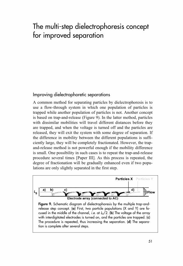
Improving dielectrophoretic separations

A common method for separating particles by dielectrophoresis is to use a flow-through system in which one population of particles is trapped while another population of particles is not. Another concept is based on trap-and-release (Figure 9). In the latter method, particles with dissimilar mobilities will travel different distances before they are trapped, and when the voltage is turned off and the particles are released, they will exit the system with some degree of separation. If the difference in mobility between the different populations is suffi-ciently large, they will be completely fractionated. However, the trap-and-release method is not powerful enough if the mobility difference is small. One possibility in such cases is to repeat the trap-and-release procedure several times [Paper III]. As this process is repeated, the degree of fractionation will be gradually enhanced even if two popu-lations are only slightly separated in the first step.

Figure 9. Schematic diagram of dielectrophoresis by the multiple trap-and-release step concept. (a) First, two particle populations (X and Y) are fo-cused in the middle of the channel, i.e. at L0/2. (b) The voltage of the array with interdigitated electrodes is turned on, and the particles are trapped. (c) The procedure is repeated, thus increasing the separation. (d) The separa-tion is complete after several steps.

52

Dielectrophoretic resolution and selectivity

To quantify the degree of fractionation obtained with the proposed method using multiple steps, a value for the “dielectrophoretic resolu-tion” (RDEP) is defined as [Paper III]:

DEPA B

3dRw w

=+

(18)

where d is the distance between the two centers of each particle popu-lation, and w is the distance between the particles most far apart with-in each population. It may either be written as a function of number of separation steps

DEP DEP( ) RR N C N= ⋅ (19)

or as a function of “dielectrophoretic selectivity”, αDEP ,

abm abmE Fo `αα α= ⋅ (20)

where αDEP , is defined as

abmIu abmIvabm

abmIu

ϑ ϑα

ϑ−

= , abmIu abmIvϑ ϑ> (21)

The constants CR and Cα in Equations 19 and 20 are, as well as the dielectrophoretic mobilities (ϑ), describing differences in hydrodyna-mic and dielectric properties.

The term “dielectrophoretic resolution” can also be used to explore the analogy with chromatography. Using the definition in Equation 18, the two particle populations will be completely separated if RDEP > 1.5.

Enhanced separation power

As in the example calculated for the superpositioned dielectrophore-sis concept, the new method of multi-step dielectrophoresis was dem-onstrated using a model consisting of a micro-channel with electrode arrays at both the top and bottom of the channel. In this model, di-electric data for polystyrene beads suspended in deionized water were used [107]. At the start of a run, the particles are assumed to be fo-cused in the middle of the channel, and when the voltage is turned on, the particles are transported to different positions downstream in the channel. The distances the particles are displaced before reaching an electrode edge depend on their hydrodynamic and dielectric proper-

53

ties. After being trapped, they are released and re-focused in the mid-dle of the channel. If the differences in dielectrophoretic behavior be-tween different sets of particles are sufficiently large, they are com-pletely separated in a single trap-and-release cycle. If the differences are small, the procedure is repeated, leading to increased resolution as the particles move downstream in the channel (Figure 9).

Results from the calculation show that it is easier to separate parti-cles with different sizes (Figure 10) than particles with different di-electric properties, since the radius of a particle is quadratically pro-portional to its mobility, while its dielectric properties are only line-arly related to its mobility. In addition, differences in conductivity have a stronger influence on the separation possibilities than differen-ces in permittivity, in accordance with the fact that the conductivity of a particle is mainly governed by its surface properties, whereas its permittivity is determined by bulk properties.

A complete separation (i.e. RDEP > 1.5) of particles may be achie-ved in two trap-and-release cycles if there is a 5% difference in their sizes. If there is a 0.5% size difference, 20 steps are required, and with 200 steps it is possible to separate particles with a size difference as small as 0.2%. For a particle with 5 µm radius, this difference cor-responds to a 10 nm coating.

As mentioned above, differences in conductivity have a stronger impact on the separation than differences in permittivity. Arnold et al. [107] have shown that the conductivity difference between sets of boiled and unboiled COOH-coated polystyrene beads is 31%. Accor-ding to the model calculations, this difference is too small to enable complete separation with a single trap-and-release cycle. It should however be possible to separate such particles by repeating the trap-and-release cycle only once. Using four steps, the required conductiv-ity difference drops to 19%. Below this level, the separation possibili-ties are very poor. A reduction in the difference of just a few percent makes separation practically impossible.

For situations close to this limit of separation, many cycles would be required. Fifty would correspond to approximately 1500 electrode pairs (assuming that 15 electrodes are utilized in each step). For parti-cles with 5 µm radii, the required channel length would be 15 cm. This is a fairly long channel, but still feasible for a lab-on-a-chip-sys-tem [108]. If the differences in dielectric properties are smaller than the critical values required to obtain any separation, some of the val-ues for the system parameters, such as electrode width, electrode gap or voltage must be changed.

54

Figure 10. Calculated resolution as a func-tion of the number of steps applied in size-based separation. (a) Relative differences in size: 5%, 2% and 1%. (b) Relative difference in size: 0.5%. (c) Rela-tive difference in size: 0.2%.

a)

0 1 2 3 40

0.5

1

1.5

2

2.5

Number of stepsR

esol

utio

n

5 %

2 %

1 %

5 %

2 %

1 %

b)

15 20 250

0.5

1

1.5

2

2.5

Number of steps

Res

olut

ion

0.5 %

c)

180 200 2200

0.5

1

1.5

2

2.5

Number of steps

Res

olut

ion

0.2 %

55

Dielectrophoresis calculation methods

Model particles

As previously mentioned, the calculations demonstrating the propo-sed concepts were performed using E. coli and polystyrene beads as model particles, with dielectric and morphological data obtained from the literature [107, 109]. Using these data, the mobilities could be cal-culated [76, 110, 111]. The results are shown in Figure 11. The eva-luations were made by calculating the trajectories of the model parti-cles. To obtain the trajectories, the electric fields and fluid velocities in different parts of the system were determined using the finite ele-ment method in combination with a numerical method for forward stepping.

Model chambers

The model channel in which the model separations were performed has a rectangular cross-section with a much greater width than height, thus allowing the calculations to be performed in a 2D plane in the di-rection of the flow. Both the top and bottom of the channel are cov-ered with an array of interdigitated electrodes [101–104]. The two ar-rays are connected to different signal generators, thus allowing differ-ent frequencies to be applied to the top and the bottom. This is useful if superpositioned fields are utilized. The electrodes in each array are connected in pairs so that the voltage phase angle between two adja-cent electrodes is 180°.

56

a)

102 104 106 108 1010

-2

-1

0

1

2

3x 10-11

Frequency [Hz]

Mob

ility

of E

. col

i [m

4 V-2s-1

]

2.3 mS/cm

1.3 mS/cm

b)

102 104 106 108 1010

-1.5

-1

-0.5

0

0.5

1

x 10-18

Frequency [Hz]

Mob

ility

of b

ead

[m4 V-2

s-1]

Figure 11. Calculated dielectrophoretic mobility for (a) E. coli in suspen-sion media with different conductivity (1.3 mS/cm and 2.3 mS/cm), and (b) a polystyrene bead (conductivity 2.0 μS/cm, relative permittivity 2.5 and a diameter of 10 μm) in deionized water (conductivity 0.66 μS/cm, relative permittivity 80 and viscosity 1·10–3 kg/m3s), as a function of fre-quency.

57

Calculation procedure

The calculation procedure included three steps. First the electric po-tentials at all positions in the model system were calculated. Using that information, the gradient of the squared electric field could be determined. Secondly, the fluid flow in all positions had to be deter-mined. Combining the data from the first and second steps, the parti-cle trajectories could then be determined in the final step.

The gradients of the squared electric field were calculated by solv-ing the Laplace equation for the electric potential, using the finite ele-ment method and standard boundary conditions [101]. In this method, the area is first divided into small elements using a mesh of tetrahe-dron units. The mesh units are smaller near the electrode edges, and grow with distance from the edges. The mesh was created in 3D using Fluent’s mesh generation software Gambit (Fluent, Inc., USA), which also allowed different boundary conditions to be applied. The meshes were refined adaptively and emerged in FemLego [56] during the computation procedure. When the electric potentials in all elements had been calculated, the gradients could be calculated. An example of the appearance of the electric potential and the electric field is dis-played in Figure 12 and Figure 13.

Plots were created in FemLab (Comsol AB, Sweden) using the fi-nite element method with the same boundary conditions as in the cal-culations used for determining the particle trajectories.

The velocity of the fluid can be calculated from the Navier-Stokes momentum balance and the mass conservation. In the model systems used in the studies underlying this thesis, the dimensions are small, and thus the flow can be assumed to be laminar. The simple geometry then allows the Navier-Stokes equations to be solved analytically. The analytical solution for the flow is the well-known parabolic pro-file.

Finally, the Forward Euler method was used to compute and trace the position of a single particle. In that method, a small step is made in the direction of the force. From the new point, another small step is taken in the direction of the force at that point. This is repeated until the particles are positioned at a distance from the wall approximately equal to their radii. MatLab (The MatWorks Inc, USA) was used to plot the trajectories of the particles.

To simplify the calculations and allow the results of different cal-culations to be easily compared, the equations were used in a dimen-sionless form, which facilitates rescaling.

58

electrode electrode electrode

Figure 12. The electric potential (equipotential lines) and the direction of the electric field (arrows) in the unit cell used in Paper III. Note that the ar-rows do not indicate the value of the field strength, but only the direction.

electrode electrode electrode

Figure 13. The electric field (lines indicate positions with equivalent elec-tric field strength) and the direction of the gradient of the squared electric field (arrows) in the unit cell used in Paper III. Note that the arrows do not indicate the value of the gradient of the squared electric field strength, but only its direction.

59

Concentrated suspensions

In the calculations supporting the two new concepts, the suspensions were assumed to be sufficiently dilute to allow particle-particle inter-actions to be neglected. However, to obtain more correct predictions of the behavior of concentrated particles, a new method was also as-sessed to account for motions induced by inter-particle forces [Paper IV]. The method proved to have high levels of efficiency and accu-racy. Furthermore, it is based on a molecular dynamics approach [112], making it possible to consider several different forces (hydro-dynamic, electrostatic and dielectrophoretic) without making the cal-culations too time-consuming. In this way, the behavior of a concen-trated suspension of polarizable particles may be predicted. The well known formation of pearl-chain structures (Figure A2.3) was also in-vestigated (Figure 14).

Calculated results show that the larger the particles are, the more readily they form pearl-chains, in accordance with theoretical consid-erations, since larger particles can have larger dipole moments. The results also show that particles tend to avoid forming pearl-chains if the electric field gradient is very large, even if they are close to each other. This means that pearl-chain formation is less likely to occur close to the electrode edges, which is also the case for the bulk flow region where the dielectrophoretic force is weak. Pearl-chain forma-tion should be more pronounced at a distance somewhat away from the electrodes, but the residence time at this position is rather short. Pearl-chain formation takes some time, thus it should not be a limit-ing factor in a trap-and-release system.

The dielectrophoretic behavior at pointed electrodes has been quantitatively verified through tentative dielectrophoresis experi-ments, as described in Appendix 3, in which experiments with poly-styrene beads at interdigitated electrodes are also described.

60

Figure 14. Calculated predic-tions of the behavior of polari-zable particles between two pointed electrodes (gray). Com-pare with the photographs in Figure A2.3. (a) Initial distribu-tion of particles. (b) Pearl chains are forming. (c) The pearl chains move toward the electrode tips where the dielec-tric force is strongest.

a)

0 10

1

b)

0 10

1

c)

0 10

1

61

The cross-flow filtration method for conductivity measurements

Gentle pre-handling of cells

When handling living cells, trapping problems may occur because the cells normally require a surrounding matrix with at least moderate conductivity [113, 114]. With a high conductivity medium, the at-tracting dielectrophoretic motion may become low or be lost comple-tely [115]. This problem may be solved by diluting the suspension medium, but many cells are sensitive to conductivity changes, and if viable cells are required for downstream use, it is of great importance to avoid exposing the cells to an environment of too low conductivity.

To obtain good quality predictions regarding dielectrophoretic be-havior, relevant values of dielectric properties such as conductivity must be available. Cross-flow filtration is suitable for handling sus-pensions of bacteria and yeast [116] and it reduces the osmotic shock [113, 114] that is normally induced when standard conductivity meas-urement procedures, which include repetitive centrifugation and re-suspension, are employed [96, 113, 117].

Isoconductance point

The conductivity of a particle suspension depends not only on the suspension medium, but is also affected by the suspended particles. A method for determining the conductivity of particles is to vary the conductivity of the medium until it reaches the same value as the con-ductivity of the suspension [117]. This value is commonly referred to as the isoconductance point, because here the conductivity of the sus-pension is the same as the conductivity of the particles. A great ad-vantage of using this method is that it is independent of the particle

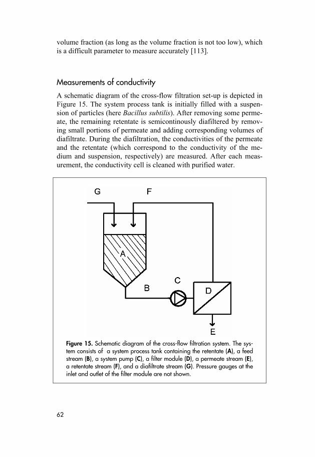
62

volume fraction (as long as the volume fraction is not too low), which is a difficult parameter to measure accurately [113].

Measurements of conductivity

A schematic diagram of the cross-flow filtration set-up is depicted in Figure 15. The system process tank is initially filled with a suspen-sion of particles (here Bacillus subtilis). After removing some perme-ate, the remaining retentate is semicontinously diafiltered by remov-ing small portions of permeate and adding corresponding volumes of diafiltrate. During the diafiltration, the conductivities of the permeate and the retentate (which correspond to the conductivity of the me-dium and suspension, respectively) are measured. After each meas-urement, the conductivity cell is cleaned with purified water.

Figure 15. Schematic diagram of the cross-flow filtration system. The sys-tem consists of a system process tank containing the retentate (A), a feed stream (B), a system pump (C), a filter module (D), a permeate stream (E), a retentate stream (F), and a diafiltrate stream (G). Pressure gauges at the inlet and outlet of the filter module are not shown.

63

Conductivity of gently treated cells

The difference between the conductivity of the suspension and the medium is plotted as a function of the conductivity of the medium. When the difference is zero, the conductivities of the medium, sus-pension and bacteria are equal [117]. Hence, the isoconductance point is to be found at the intersection between the x-axis and the plotted curve. Using the least square-method, a straight line is fitted to the data (Figure 16). The intercept of the curve in our case was found to be 270 ± 52 µS/cm, and the slope –0.042 ± 0.006 (both with 95 % confidence limits). Three separate experiments with three different B. subtilis cultures yielded a conductivity of 7000 ± 1500 µS/cm (using a one-sample t-test with 95 % confidence limits). Previous reports on the conductivity of B. subtilis [96] state a value of 935 ± 96 µS/cm. Hence, the value obtained in this study is almost an order of a magni-tude higher than previously reported. This discrepancy is believed to be due to differences in cell treatments during the measurements. The cross-flow filtration allows the osmotic potential of the suspension medium to be changed gradually from the starting value, thereby ex-posing the micro-organisms to less osmotic stress.

64

Figure 16. Conductivity difference between retentate and permeate during cross-flow filtration as a function of the conductivity of the permeate. The straight line (solid) is fitted to data (coefficient of determination, R2 = 0.974). The isoconductance point is at the intersection between the line and the x-axis (6600 μS/cm). The two curved (dashed) lines show the 95 % confidence limit prediction intervals.

65

Conclusions and future outlook

The studies this thesis is based upon have demonstrated that chroma-tograms can be predicted with good precision using both the iterative method and the finite element method. A semi-empirical two-parame-ter method for estimating the partitioning of the analytes between the mobile and stationary phases proved to be sufficient for predicting re-tention times using the iterative method. The relative differences be-tween the predicted and experimental values were only 1 %. The fi-nite element method was more time-consuming and more difficult to use, but the difference could be reduced to merely 0.1 %. When using the finite element method, a three-parameter partition model was uti-lized, which helped to improve the results, but the parameter values may be more difficult to interpret than the parameters in the two-para-meter model.

A possible option for improving the concordance between the cal-culated and experimentally acquired results is to improve the instru-mental control. With more precise temperature control in the oven, the isothermally acquired data would be more accurate, and devia-tions between the predicted and measured retention times may be re-duced. Further studies of repeatability versus reproducibility, e.g. co-lumn-to-column discrepancies, should also help to improve retention predictions.

The finite element method also displayed promising results for the predictions of peak widths. Since the peak widths during idealized conditions could be determined, studies of deviations between calcu-lated and empirically determined peak widths may give important clues regarding non-ideal behavior and extra-column effects. Further-more, in the finite element method, retaining mechanisms such as ad-sorption isotherms, or disturbing effects such as sample overload, may be added. This could facilitate realistic calculations of peak skewness and predictions of inverse-chromatography behavior.

66

The trapping capacity (quantified by the breakthrough volume) of an open tubular trap coated with a very thick film of sorbent is direct-ly dependent on the volume of sorbent stationary phase in the trap. It was shown, both theoretically and experimentally, that for a given gas flow rate and phase volume ratio, the analyte dispersion does not in practice depend on the inner diameter of the trapping column. The breakthrough volume increases in proportion to the square of the in-crease in inner diameter if the phase ratio is kept constant. These rela-tionships can be used for optimization purposes when preparing open tubular traps for applications such as concentrating reactive and ther-mally instable trace components or very volatile analytes.

The concept of trapping particles with superpositioned dielectro-phoresis is particularly useful in cases where the conductivity of the suspension medium has to be high. The overall flow rates and throughput are low under such conditions, but this may still be accep-table when dealing with living cells and where a high survival rate of the cells is a key priority. Operation with superpositioned fields also offers greater scope for fine tuning and improved selective trapping of particles according to shape and dielectric properties.

The multi-step dielectrophoresis concept based on repetitive di-electrophoretic trap-and-release cycles in a flow system could provide entirely new possibilities for applications such as production of mo-nodisperse materials or cell separation. Model calculations for poly-styrene beads predict that it should be possible to obtain complete separation of particles with a 0.2 % size difference by performing approximately 200 trap-and-release cycles. Since the particles are refocused in every cycle, the resolution increases linearly with the number of cycles. The improved separation power could be of great interest for fractionating particles with small differences in surface conductivity, and applications can be envisioned in connection with flow-based affinity-based assays. There seems to be a limiting value of conductivity differences, below which no separation can be ob-tained. For the model system used for calculations in this thesis, this limiting value was an 18 % difference in conductivity.

When determining the conductivity of living cells, incorporating cross-flow filtration should result in more accurate values and lower degrees of cell destruction than conventional methods. It should be possible to miniaturize the equipment and to operate it in a continu-ous mode, which would allow it to be integrated with dielectropho-retic chip-based separation systems. This may be particularly useful when manual handling must be avoided, e.g. when dealing with haz-

67

ardous organisms or in cases where only very small amounts of mate-rial are available.

The preliminary practical tests that have been performed have shown that living cells behaved as predicted by theoretical models. In conclusion, the developed methods have shown promising potential for improving separations. However, further experimental work is now required to validate the proposed concepts.

68

69

References

[1] L. Choi, “Secretory and extracellular production of recombinant proteins using Escherichia coli”, Applied Microbiology and Biotechnology 64 (2004) 625–635.

[2] G. A. Eiceman, J. Gardea-Torresdey, F. Dorman, E. Overton, A. Bhushan, H. P. Dharmasena, “Gas chro-matography”, Analytical Chemistry 78 (2006) 3985–3996.

[3] S. Vezzani, P. Moretti, G. Castello, “Prediction of the separation number of capillary columns in pro-grammed temperature gas chromatographic analysis”, Analytica Chimica Acta 599 (2007) 151–161.

[4] H. W. Habgood, W. E. Harris, “Retention temperature and column efficiency in programmed temperature gas chromatography”, Analytical Chemistry 32 (1960) 450–453.

[5] E. V. Dose, “Off-line optimization of gas chroma-tographic temperature programs”, Analytical Chemis-try 59 (1987) 2420–2423.

[6] E. V. Dose, “Simulation of gas-chromatographic re-tention and peak width using thermodynamic reten-tion indexes”, Analytical Chemistry 59 (1987) 2414–2419.

[7] E. E. Akporhonor, S. Le Vent S, D. R. Taylor, “Cal-culation of programmed temperature gas chromatog-raphy characteristics from isothermal data – I. Theory and computational procedures”, Journal of Chroma-tography A 405 (1987) 67–76

70

[8] E. E. Akporhonor, S. Le Vent S, D. R. Taylor, “Cal-culation of programmed temperature gas chromatog-raphy characteristics from isothermal data – II. Pre-dicted retention times and elution temperatures”, Journal of Chromatography A 463 (1989) 271–280.

[9] E. E. Akporhonor, S. Le Vent S, D. R. Taylor, “Cal-culation of programmed temperature gas chroma-tographic characteristics from isothermal data – III. Predicted retention indices and equivalent tempera-tures”, Journal of Chromatography A 504 (1990) 269–278.

[10] T. I. Al-Bajjari, S. Le Vent, D. R Taylor, “Calculation of programmed temperature gas chromatography characteristics from isothermal data – IV. Prediction of peak widths”, Journal of Chromatography A 683 (1994) 367–376.

[11] D. E. Bautz, J. W. Dolan, W. D. Raddatz, L. R. Sny-der, “Computer simulation (based on a linear-elution-strength approximation) as an aid for optimizing sepa-rations by programmed-temperature gas chromatogra-phy“, Analytical Chemistry 62 (1990) 1560–1567.

[12] D. E. Bautz, J. W. Dolan, L. R. Snyder, “Computer-simulation as an aid in method development for gas-chromatography – 1. The accurate prediction of sepa-ration as a function of experimental conditions”, Journal of Chromatography 541 (1991) 1–19.

[13] L. R. Snyder, D. E. Bautz, J. W. Dolan, “Computer-simulation as an aid in method development for gas-chromatography – 3. Examples of its application”, Journal of Chromatography A 541 (1991) 35–58.

[14] H. Snijders, H.-G. Janssen, C. Cramers, “Optimization of temperature-programmed gas chromatographic separations – 1. Prediction of retention times and peak widths from retention indices”, Journal of Chroma-tography A 718 (1995) 339–355.

71

[15] H. Snijders, H.-G. Janssen, C. Cramers, “Optimization of temperature-programmed gas chromatographic separations – 2. Off-line simplex optimization and column selection”, Journal of Chromatography A 756 (1996) 175–183.

[16] G. Castello, P. Moretti, S. Vezzani, “Comparison of different methods for the prediction of retention times in programmed-temperature gas-chromatography“, Journal of Chromatography 635 (1993) 103–111.

[17] S. Vezzani, P. Moretti, G. Castello, “Fast and accurate method for the automatic prediction of programmed-temperature retention times”, Journal of Chromatog-raphy A 677 (1994) 331–343.

[18] S. Vezzani, P. Moretti, G. Castello, G. Travaini, “Pre-diction of the resolution of capillary columns in dif-ferent conditions of inlet pressure and temperature”, Journal of Chromatography A 1026 (2004) 201–221.

[19] S Vezzani, P Moretti, M Mazzi, G Castello, “Predic-tion of retention times in linear gradient temperature and pressure programmed analysis on capillary col-umns”, Journal of Chromatography A 1055 (2004) 151–158.

[20] G. Castello, S. Vezzani, P. Moretti, “Comparison of the behaviour of gas-liquid and gas-liquid-solid capil-lary columns through the determination of thermody-namic characteristics”, Journal of Chromatography 742 (1996) 151–160.

[21] S. Vezzani, P. Moretti, G. Castello, “Automatic pre-diction of retention times in multi-linear programmed temperature analyses”, Journal of Chromatography A 767 (1997) 115–125.

[22] P. Moretti, S. Vezzani, E. Garrone, G. Castello, “Evaluation and prediction of the shape of gas chro-matographic peaks”, Journal of Chromatography A 1038 (2004) 171–181.

72

[23] F. R. Gonzalez, A. M. Nardillo, “Theoretical and practical aspects of flow control in programmed-temperature gas chromatography”, Journal of Chro-matography A 757 (1997) 97–107.

[24] F. R. Gonzalez, A. M Nardillo, “Retention in multistep programmed-temperature gas chromatogra-phy and flow control. Linear head pressure pro-grams”, Journal of Chromatography A 757 (1997) 109–118.

[25] F. R. Gonzalez, A. M. Nardillo, “Integration of the equation of peak motion in programmed-pressure and -temperature gas chromatography”, Journal of Chro-matography A 766 (1997) 147–152.

[26] F. R. Gonzalez, A. M. Nardillo, “Aspects of the elu-tion order inversion by pressure changes in pro-grammed-temperature gas Chromatography”, Journal of Chromatography A 779 (1997) 263–274.

[27] F. R. Gonzalez, J. L. Alessandrini, A. M. Nardillo, “Considerations on the dependence of gas-liquid chromatographic retention of n-alkanes with the car-bon number”, Journal of Chromatography A 810 (1998) 105–117.

[28] F. R. Gonzalez, A. M. Nardillo, “Retention index in temperature-programmed gas Chromatography”, Journal of Chromatography A 842 (1999) 29–49.

[29] F. R. Gonzalez, J. L. Alessandrini, A. M. Nardillo, “Revision of a theoretical expression for gas–liquid chromatographic retention”, Journal of Chromatog-raphy A 852 (1999) 583–588.

[30] F. R. Gonzalez, “Interpreting the gas chromatographic retention of n-alkanes”, Journal of Chromatography A 873 (2000) 209–219.

[31] F. R. Gonzalez, L. G. Gagliardi, “Distribution coeffi-cients of n-alkanes measured on wall-coated capillary columns” Journal of Chromatography A 879 (2000) 157–168.

73

[32] F. R. Gonzalez, R. C. Castells, A. M. Nardillo, “Be-havior of n-alkanes on poly(oxyethylene) capillary columns. Evaluation of interfacial effects”, Journal of Chromatography A 927 (2001) 111–120.

[33] F. R. Gonzalez, “Considerations on the temperature dependence of the gas-liquid chromatographic reten-tion”, Journal of Chromatography A 942 (2002) 211–221.

[34] F. R. Gonzalez, “Application of capillary gas chroma-tography to studies on solvation thermodynamics”, Journal of Chromatography A 1037 (2004) 233–253.

[35] Z. Wu, “Retention simulation in gas chromatogra-phy”, Journal of Chromatography A 840 (1999) 137–143.

[36] R. C. Castells, E. L. Arancibia, “Regression against temperature of gas-chromatographic retention data”, Journal of Chromatography 504 (1990) 45–53.

[37] R. C. Castells, “Determination of gas-liquid partition coefficients by gas chromatography “, Journal of Chromatography A 1037 (2004) 223–231.

[38] J. P. Chen, L. Zhang, Y. Tian, L. Wang, “Novel ap-proach for the prediction of retention times in operat-ing parameter programmed gas-liquid chromatogra-phy with capillary columns”, Journal of Chromatog-raphy A 795 (1998) 305–317.

[39] J. P. Chen, X. M. Liang, Q. Zhang, L. F. Zhang, “Pre-diction of GC retention values under various column temperature conditions from temperature programmed data”, Chromatographia 53 (2001) 539–547.

[40] J. P. Chen, X. M. Liang, Q. Zhang, L. F. Zhang, “An empirical equation for the calculation of retention time with extrapolation of temperature in gas chroma-tography“, Chromatographia 53 (2001) 548–552.

74

[41] L. F. Dorman, P. D. Schettler, C. M. English, D. V. Patwardhan, “Predicting gas chromatographic separa-tion and stationary-phase selectivity using computer modeling”, Analytical Chemistry 74 (2002) 2133–2138.

[42] F. Luan, C. Xue, R. Zhang, C. Zhao, M. Liu, Z. Hu, B. Fan, “Prediction of retention time of a variety of volatile organic compounds based on the heuristic method and support vector machine”, Analytica Chimica Acta 537 (2005) 101–110.

[43] M. J. E. Golay, in: D. H. Desty (Ed) “Theory of chromatography in open and coated tubular columns with round and rectangular cross-sections”, Gas chromatograpy, Butterworth, London, UK (1958) pp. 36–55.

[44] P. J. Karol, “Chromatogram statistical moments from columns of finite length”, Journal of Chromatography 445 (1988) 207–210.

[45] P. J. Karol, “A different perspective on the theoretical plate in equilibrium chromatography”, Analytical chemistry 61 (1989) 1937–1941.

[46] E. Kučera, “Contribution to the theory of chromatog-raphy – Linear non-equilibrium elution chromatogra-phy “, Journal of Chromatography 19 (1965) 237–248.

[47] K. J. Ward, S. C. Kaliaguine, P. A. Tanguy, G. Jean, “Numerical simulation of a chromatograph column – Linear case”, Industrial & Engineering Chemistry Re-search 27 (1988) 1474–1480.

[48] J. Å. Jönsson, “Elution curves and statistical moments in non-ideal, linear chromatography”, Chroma-tographia 18 (1984) 427–433.

[49] T. Gu, G.-J. Tsai, G. T. Tsao, “New approach to a general nonlinear multicomponent Chromatography”, AIChE Journal 36 (1990) 784–788.

75

[50] W. A. Peters, Jr., “The efficiency and capacity of fractionating columns”, Journal of Industrial & Engi-neering Chemistry 14 (1922) 476–479.

[51] J. J. van Deemter, F. J. Zuiderweg, A. Klinkenberg, “Longitudinal diffusion and resistance to mass trans-fer as causes of nonideality in chromatography”, Chemical Engineering Science 5 (1956) 271–289.

[52] S. Golshan-Shirazi, G. Guiochon, “Analytical solution for the ideal model of chromatography in the case of a Langmuir isotherm”, Analytical Chemistry 60 (1988) 2364–2374.

[53] E. N. Fuller, P. D. Schettler, J. C. Giddings, “A new method for prediction of binary gas-phase diffusion coefficients”, Industrial and Engineering Chemistry 58 (1966) 19–27.

[54] O. Rübenkönig, The Finite Difference Method (FDM) - An introduction, Albert Ludwigs University of Freiburg, Germany (2006).

[55] D. L. Logan, A First Course in the Finite Element Method, PWS Publishing, Boston, USA (1992).

[56] G. Amberg, R. Tönhardt, C. Winkler, “Finite element simulations using symbolic computing”, Mathematics and Computers in Simulation 49 (1999) 257–274.

[57] F. Chen, E. C. Drumm, G. Guiochon, “Stress distribu-tion and dimensional changes in chromatographic columns”, Journal of Chromatography A 1083 (2005) 68–79.

[58] G. P. Todd, R. H. Haschemeyer, “Generalized finite element solution to one-dimensional flux problems”, Biophysical Chemistry 17 (1983) 321–326.

[59] L. Yajiang, W. Juan, F. Jicai, S. Xiaoqin, “Finite ele-ment modeling of hydrogen diffusion in fusion zone of HQ130 high strength”, Journal of Materials Proc-essing Technology 161 (2005) 423–429.

76

[60] O. Shipilova, H. Haario, A. Smolanski, “Particle transport method for convection problems with reac-tion and diffusion”, International Journal for Numeri-cal Methods in Fluids 54 (2007) 1215–1238.

[61] R. L. Grob, E. F. Barry, S. Leepipatpiboon, J. M. Ombaba, L. A. Colon, “Computer-assisted enhance-ment of gas chromatographic principles for the teach-ing laboratory. Prediction of retention data and chro-matographic separation”, Journal of Chromatographic Science 30 (1992) 177–183.

[61] Y. Williamson, J. M. Davis, “Validation of theory of n-column separations with gas chromatograms pre-dicted by commercial software”, Journal of Separa-tion Science 30 (2007) 74–85.

[62] J. E. Quintanilla-López, R. Lebrón-Aguilar, J. A. Gar-cía-Domínguez, “Hold-up time in gas Chromatogra-phy V. Dependence of the retention of n-alkanes on the chromatographic variables in isothermal gas Chromatography”, Journal of Chromatography A 878 (2000) 125–135.

[63] A. Bemgård, A. Colmsjö, K. Wrangskog, “Prediction of Temperature-Programmed Retention Indexes for Polynuclear Aromatic-Hydrocarbons in Gas-Chromatography“, Analytical Chemistry 66 (1994) 4288–4294.

[64] C.-E. Boström, P. Gerde, A. Hanberg, B. Jernström, C. Johansson, T. Kyrklund, A. Rannung, M. Törn-qvist, K. Victorin, R. Westerholm, “Cancer risk as-sessment, indicators, and guidelines for polycyclic aromatic hydrocarbons in the ambient air”, Environ-mental Health Perspectives 110 (2002) 451–488.

[65] C. L. Arthur, J. Pawliszyn, “Solid phase microextrac-tion with thermal desorption using fused silica optical fibers”, Analytical Chemistry 62 (1990) 2145–2148.

[66] J. Pettersson, A. Kloskowski, C. Zaniol and J. Ro-eraade, “Automated High Capacity Sorption Probe for Extraction of Ultra Trace Components from Aqueous Samples”, Journal of Chromatography A 1033 (2004) 339–347.

77

[67] E. Baltussen, F. David, P. Sandra, C. Cramers, “On the performance and inertness of different materials used for the enrichment of sulfur compounds from air and gaseous samples”, Journal of Chromatography A 864 (1999) 345–350.

[68] E. Baltussen, P. Sandra, F. David, H.-G. Janssen, C. Cramers, “Study into the Equilibrium Mechanism be-tween Water and Poly(dimethylsiloxane) for Very Apolar Solutes: Adsorption or Sorption?”, Analytical Chemistry 71 (1999) 5213–5216.

[69] E. Baltussen, C. A. Cramers, P. J. F. Sandra, “Sorp-tive sample preparation - a review”, Analytical and Bioanalytical Chemistry 373 (2002) 3–22.

[70] P. Lövkvist, J. Å. Jönsson, “Capacity of sampling and preconcentration columns with a low number of theo-retical plates”, Analytical Chemistry 59 (1987) 818–821.

[71] E. K. Ortner, E. R. Rohwer, “Trace analysis of semi-volatile organic air pollutants using thick film silicone rubber traps with capillary gas chromatography”, Journal of High Resolution Chromatography 19 (1996) 339–344.

[72] M. S. Krieger, R. A. Hites, “Diffusion denuder for the collection of semivolatile organic compounds”, Envi-ronmental Science & Technology 26 (1992) 1551–1555.

[73] S. Blomberg, J. Roeraade, “Preparative capillary gas chromatography. II. Fraction collection on traps coated with a very thick film of immobilized station-ary phase”, Journal of Chromatography 394 (1987) 443–453.

[74] A. Kloskowski, J. Pettersson and J. Roeraade, “Thick Film Traps with an Irregular Film – Preparation and Evaluation”, Journal of Chromatography A 1035 (2004) 159–165.

[75] H. A. Pohl, “The motion and percipitation of suspen-soids in divergent electric fields”, Journal of Applied Physics 22 (1951) 869–871.

78

[76] H. Morgan, N. G. Green, AC Electrokinetics: colloids and nanoparticles, Research Studies Press, Baldock, Hertfordshire, UK (2003) p. 297.

[77] D. Pappas, K. Wang, “Cellular separations: A review of new challenges in analytical chemistry”, Analytica Chimica Acta 601 (2007) 26–35.

[78] H. Andersson, A. van den Berg, “Microfluidic devices for cellomics: a review”, Sensors and Actuators B 92 (2003) 315–325.

[79] D. Erickson, D. Li, “Integrated microfluidic devices”, Analytica Chimica Acta 507 (2004) 11–26.

[80] C. Yi, C. -W. Li, S. Ji, M. Yang, “Microfluidics tech-nology for manipulation and analysis of biological cells”, Analytica Chimica Acta 560 (2006) 1–23.

[81] P. S. Dittrich, K. Tachikawa, A. Manz, “Micro total analysis systems. Latest advancements and trends”, Analytical Chemistry 78 (2006) 3887–3907.

[82] M. P. Hughes, “Strategies for dielectrophoretic sepa-ration in laboratory-on-a-chip systems”, Electropho-resis, 23 (2002) 2569–2582.

[83] P. R. C. Gascoyne, J. Vykoukai, “Particle separation by dielectrophoresis”, Electrophoresis 23 (2002) 1973–1983.

[84] E. G. Cen, C. Dalton, Y. Li, S. Adamia, L. M. Pilar-ski, K. V. I. S. Kaler, “A combined dielectrophoresis, traveling wave dielectrophoresis and electrorotation microchip for the manipulation and characterization of human malignant cells”, Journal of Microbiologi-cal Methods 58 (2004) 387–401.

[85] H. J. Tanke, M. van der Keur, “Selection of defined cell types by flow-cytometric cell sorting”, Tibtech 11 (1992) 55–62.

[86] K. Cheung, S. Gawad, P. Renaud, “Impedance spec-troscopy flow cytometry – On-chip label-free cell dif-ferentiation”, Cytometry A 65A (2005) 124–132.

79

[87] P. Reschiglian, A. Zattoni, B. Roda, E. Michelini, A. Roda, “Field-flow fractionation and biotechnology”, TRENDS in Biotechnology 23 (2005) 475–483.

[88] X. B. Wang, J. Vykoukal, F. F. Becker, P. R. Gas-coyne, “Separation of polystyrene microbeads using dielectrophoretic gravitational field-flow-fractionation”, Biophysical Journal 74 (1998) 2689–2701.

[89] X. B. Wang, J. Yang, Y. Huang, J. Vykoukal, F. F. Becker, P. R. Gascoyne, “Cell separation by dielec-trophoretic field-flow-fractionation”, Analytical Chemistry 72 (2000) 832–839.

[90] R. Pethig, G. H. Markx, “Applications of dielectro-phoresis in biotechnology”, Tibtech 15 (1997) 426–432.

[91] N. Gadish, J. Voldman, “High-throughput positive-dielectrophoretic bioparticle microconcentrator”, Ana-lytical Chemistry 78 (2006) 7870–7876.

[92] A. Heeren, C. P. Luo, W. Henschel, M. Fleischer, D. P. Kern, “Manipulation of micro- and nano-particles by electro-osmosis and dielectrophoresis”, Microelec-tronic Engineering 84 (2007) 1706–1709.

[93] C. H. Kua, Y. C. Lam, I. Rodriguez, C. Yang, K. Youcef-Toumi, “Dynamic cell fractionation and transportation using moving dielectrophoresis”, Ana-lytical Chemistry 79 (2007) 6975–6987.

[94] S. K. Ravula, D. W. Branch, C. D. James, R. J. Town-send, M. Hill, G. Kaduchak, M. Ward, I. Brener, “A microfluidic system combining acoustic and dielec-trophoretic particle preconcentration and focusing”, Sensors and Actuators B: Chemical (2007), in press.

[95] T. B. Christensen, C. M. Pedersen, D. D. Bang, A. Wolff, “Sample preparation by cell guiding using negative dielectrophoresis”, Microelectronic Engi-neering 84 (2007) 1690–1693.

80

[96] G. H. Markx, Y. Huang, X.-F. Zhou, R. Pethig, “Di-electrophoretic characterization and separation of mi-croorganisms”, Microbiology 140 (1994) 585–591.

[97] A. Docoslis, N. Kalogerakis, L. A. Behie, K. V. I. S. Kaler, “A novel dielectrophoresis-based device for the selective retention of viable cells in cell culture me-dia”, Biotechnology and Bioengineering 54 (1997) 239–250.

[98] M. P. Hughes, R. Pethig, X.-B. Wang, “Dielectropho-retic forces on particles in travelling electric fields”, Journal of Physics D: Applied Physics 29 (1996) 474–482.

[99] R. Pethig, M. S. Talary, R. S. Lee, “Enhancing travel-ing-wave dielectrophoresis with signal superposition”, IEEE Engineering in Medicine and Biology Magazine 22 (2003) 43–50.

[100] M. Urdaneta, E. Smela, “Multiple frequency dielec-trophoresis”, Electrophoresis 28 (2007), 3145–3155

[101] N. G. Green, A. Ramos, H. Morgan, “Numerical solu-tion of the dielectrophoretic and travelling wave forces for interdigitated electrode arrays using the fi-nite element method”, Journal of Electrostatics 56 (2002) 235–254.

[102] D. Holmes, N. G. Green, H. Morgan, “Microdevices for dielectrophoretic flow-through cell separation”, IEEE Engineering in Medicine and Biology Magazine 22 (2003) 85–90.

[103] H. Li, R. Bashir, “On the design and optimization of micro-fluidic dielectrophoretic devices – a dynamic simulation study”, Biomedical Microdevices 6 (2004) 289–295.

[104] M. Suzuki, T. Yasukawa, Y. Mase, D. Oyamatsu, H. Shiku, T. Matsue, “Dielectrophoretic micropatterning with microparticle monolayers covalently linked to glass surfaces”, Langmuir 20 (2004) 11005–11011.

81

[105] M. Castellarnau, A. Errachid, C. Madrid, A. Juárez, J. Samitier, “Dielectrophoresis as a tool to characterize and differentiate isogenic mutants of Esherichia coli”, Biophysical Journal 91 (2006) 3937–3945.

[106] M. Varshney, Y. Li, “Double interdigitated array mi-croelectrode-based impedance biosensor for detection of viable Escherichia coli O157:H7 in growth me-dium”, Talanta (2007), in press.

[107] W. M. Arnold, H. P. Schwan, U. Zimmermann, “Sur-face conductance and other properties of latex parti-cles measured by electrorotation”, Journal of Physical Chemistry 91 (1987) 5093–5098.

[108] A. Manz, H. Becker, Microsystem Technology in Chemistry and Life Sciences, Springer-Verlag Berlin Heidelberg, Germany (1999).

[109] K. Asami, T. Hanai, N. Koizumi, “Dielectric analysis of Escherichia coli suspensions in the light of the the-ory of interfacial polarization”, Biophysical Journal 31 (1980) 215–228.

[110] K. Asami, T. Yonezawa, “Dielectric behavior of non-spherical cells in culture”, Biochimica et Biophysica Acta 1245 (1995) 317–324.

[111] H. Morgan, N. G. Green, “Dielectrophoretic manipu-lation of rod-shaped particles”, Journal of Electrostat-ics 42 (1997) 279–293.

[112] M. Elimelech, J. Gregory, X. Jia, R. A. Williams, “Particle deposition and aggregation – measurement, modelling and simulation”, Journal of Chemistry and Physics 63 (1975) 2376–2394.

[113] A. van der Wal, M. Minor, W. Norde, A. J. B. Zehnder, J. Lyklema, “Conductivity and dielectric dispersion of gram-positive bacterial cells”, Journal of Colloid and Interface Science 186 (1997) 71–79.

[114] S. Morbach, R. Krämer, “Body shaping under water stress: osmosensing and osmoregulation of solute transport in bacteria”, ChemBioChem 3 (2002) 384–397.

82

[115] G. Fuhr, H. Glasser, T. Müller, T. Schnelle, “Cell manipulation and cultivation under AC electric fiels influence in highly conductive culture media”, Bio-chimica et Biophysica Acta 1201 (1994) 353–360.

[116] M. Cheryan, Ultrafiltration Handbook, Technomic Publishing Company, Inc Lancaster, PA, USA (1998) p. 527.

[117] Z. Yunus, V. Mason, C. E. Verduzco-Luque, G. H. Markx, “A simple method for the measurement of bacterial particle conductivities”, Journal of Microbi-ological Methods 51 (2002) 401–406.

Thank you for reading my thesis!

83

Appendix 1: Superpositioning of two alternating current electric fields in dielectrophoresis

The dielectrophoretic force and velocity are proportional to the gradi-ent of the squared electric field (Equation 16). For the two-dimensional case, with

φ= −∇E (A1.1)

where φ is the electric potential, the gradient of the squared electric field can be described for a 2D case (assuming that the electric field is free from rotation) as

2 2 2 22

2 22 ,φ φ φ φ φ φ φ φx x y x y x y x y y

⎛ ⎞∂ ∂ ∂ ∂ ∂ ∂ ∂ ∂∇ = + +⎜ ⎟∂ ∂ ∂ ∂ ∂ ∂ ∂ ∂ ∂ ∂⎝ ⎠

E (A1.2)

The total potential from the two fields may be written as

1 1 2 2sin( ) sin( )φ φ ω t φ ω t δ= + + (A1.3)

where φ1 and φ2 are the amplitudes of the two fields, ω is the angular frequency, t is the time, and δ is the phase shift.

Since the dielectrophoretic force is proportional to 2φ∇ ∇ , and the potential is induced by two fields with different frequencies, the total force is proportional to

( ) ( )( )( ) ( )( )

( )( )

2 21 1 2 2

2 22 21 1 2 2

21 2 1 2 1 2

sin( ) sin( )

sin ( ) sin ( )

cos( ) cos( )

φ φ ω t φ ω t δ

φ ω t φ ω t δ

φ φ ω t ω t ω t ω t δ

∇ ∇ =∇ ∇ +∇ + =

= ∇ ∇ +∇ ∇ +

+∇ ∇ ∇ − − + +

(A1.4)

To obtain the time-averaged force, the squared electric field is in-tegrated from time zero to a time T and then multiplied by 1/T.

84

( )21 2 3

0

1 dT

φ t I I IT

∇ ∇ = + +∫ (A1.5)

where

( )2 21 1 1

0

1 sin ( )dT

I φ ω t tT

⎛ ⎞= ∇ ∇⎜ ⎟

⎝ ⎠∫ (A1.6)

( )2 22 2 2

0

1 sin ( )dT

I φ ω t δ tT

⎛ ⎞= ∇ ∇ +⎜ ⎟

⎝ ⎠∫ (A1.7)

( ) ( )C 1 2 1 2 1 20 0

1 cos( )d cos( )dT T

I φ φ ω ω t δ t ω ω t δ tT

⎛ ⎞⎛ ⎞= ∇ ∇ ∇ − − − + +⎜ ⎟⎜ ⎟⎜ ⎟⎝ ⎠⎝ ⎠

∫ ∫ (A1.8) If the time 1 21/( )T ω ω− and 1 21/( )T ω ω+ , then

C 0I ≈ (A1.9)

whereas

( )21 1

12I φ≈ ∇ ∇ ⋅ (A1.10)

and

( )22 2

12I φ≈ ∇ ∇ ⋅ (A1.11)

and therefore

( ) ( ) ( )( )( )

2 2 21 1 2

0

2 21 2

1 1d 02

12

T

φ t φ φT

∇ ∇ ≈ ∇ ∇ ⋅+∇ ∇ +

= ∇ +∇

∫

E E (A1.12)

Hence, if two fields are superpositioned, the coupling term Ic may be neglected when computing the dielectrophoretic force. It is then possible to have one field with a frequency that induces positive di-electrophoresis, and another frequency that induces negative dielec-trophoresis. Furthermore, if the distance between the electrodes is sufficiently large, it is valid to approximate that the forces act inde-pendently of each other due to the intrinsically short range of the di-electrophoretic force.

85

Appendix 2: Complementary dielectrophoresis experiments

Preparation of beads and bacteria

Initial dielectrophoresis experiments have been performed to assess empirically the dielectrophoretic behavior of polystyrene beads and E. coli bacteria. A mixture of polystyrene beads with diameters of 0.5 and 2.0 µm were utilized. The beads were initially suspended in an aqueous solution, samples of the suspension were centrifuged at 5000 rpm for 3 minutes, the medium was removed, and the beads were resuspended in deionized water. Samples of beads with differing con-ductivities were prepared by adding KCl or MilliQ water to the bead suspensions.

E. coli bacteria of a genetically modified strain were cultured batch-wise, and samples were withdrawn from the culture at regular intervals. The samples were centrifuged, the supernatants were re-moved and the bacteria pellets were frozen, then washed three times with deionized water prior to dielectrophoresis. The conductivity of suspensions prepared from these bacteria was modified by adding known amounts of NaCl solution.

Open dielectrophoresis device

The experimental devices were designed to position particles at a desired spot or in different patterns. They were also designed to be easy to use, clean, and reuse.

The basic platform for the dielectrophoresis device was a glass plate equipped with thin-film Ti- or Al-electrodes, with geometries

86

dimensioned to suit the size of the particles used in the experiments. Different electrode shapes and positioning patterns were tested (tip distance 10 or 30 µm, point angle 90 or 110 degrees, and spacing 30 or 100 µm), and straight interdigitated geometries of 10 µm width and 15 µm spacing. The pointed electrodes were designed to produce a very high electric field gradient locally around the tip. The straight electrodes were tested to arrange the sample particles in rows at the edges of or between the electrodes. Single pairs and arrays of up to 50 electrodes were used.

The dielectrophoresis device was microfabricated using one-mask lithography and a 0.20 μm thick titanium layer, deposited by sputter-ing onto a 76 x 35 mm piece of standard soda-lime glass substrate, 2 mm thick, which was cleaned using standard procedures. Photolitho-graphy of a positive photo resist (Shipley-1813) was used for pattern-ing, and the excess titanium was removed by etching in buffered hy-drogen fluoride solution (5 vol-% hydrogen fluoride buffered with ammonium fluoride). The photo resist was removed in acetone and the substrate was then spin-dried. Electrical connections to the elec-trodes were made by bonding wires to the contact pads using conduc-tive epoxy glue. The substrate can be easily converted to a fluidic device by mounting a piece of PDMS with a molded channel and in/out connections on top of the electrode platform (Figure A2.1). In the experimental set-up we used, the size of an array of 100 electrode pairs was 5 x 5 mm2, and the total length of the device was approxi-mately 50 mm.

The experimental set-up consisted of the dielectrophoresis device mounted onto the table of a fluorescence microscope (Nikon eclipse E600) equipped with a digital camera (Nikon Coolpix) (Figure A2.1). To apply the electric field, a function generator (TTi TG-120) was connected to the device via the wires of the micro dielectrophoresis chip. In order to check the electric field, an oscilloscope (GW Instec GOS-620 20 MHz) was used. The particle suspension was dispensed drop-wise onto the electrode-glass system and covered with a stan-dard cover glass for light microscopy. In the experiments, sine waves at frequencies from 100 Hz up to 20 MHz and voltages from 0 to 20 V peak to peak were used. The responses of the particles to the ap-plied electric fields were studied using a fluorescence microscope. After each experiment, the plates with electrodes were washed with 70 % ethanol and MilliQ water and then dried with nitrogen gas. Cleaned in this way, the device could be used for more than 30 con-secutive experiments, with no detectable loss of performance.

87

Figure A2.1. Schematic diagram of the dielectrophoresis set-up used in the experiments. The device consists of a glass microscope slide (A) with Ti electrodes (B). The suspension (C) is deposited drop-wise directly onto the surface, and enclosed with a standard cover glass (D).

Positioning and separation of beads

Dielectrophoretic positioning of polystyrene beads in rows was per-formed using an array of interdigitated electrodes. Each sample con-tained a mixture of 2 µm and 0.5 µm diameter beads. The conductiv-ity of the sample was 8 µS/cm. At low frequency (10 kHz) the beads stuck to the electrodes. At 1.40 MHz the 2.0 µm beads were subjected to a negative dielectrophoretic force and thus became positioned in rows between the electrodes (Figure A2.2). When the frequency was increased to 4.0 MHz, the 0.5 µm beads were affected by a negative dielectrophoretic force and also positioned themselves in rows. An interaction effect was also seen, causing the particles to form pearl chains with nearby particles.

Behavior of E. coli

The dielectrophoretic behavior of E. coli cells was also demonstrated using the pointed electrodes. The bacteria were exposed to electric fields with frequencies between 10 kHz and 20 MHz. At the lower frequencies, the bacteria linearized and pearl-chains were formed

A

B

C D

88

(Figure A2.3).When the frequency was increased, the pearl-chain formation became more pronounced and the particles drifted towards the gap between the electrode tips. At higher frequencies, about 3 MHz and higher, rotation was observed and the pearl-chains seemed to become distorted following further increases in the frequency. At frequencies higher than 10–15 MHz, the bacteria changed orientation and linearized orthogonally to the field. Pearl-chains of bacteria ori-ented in the same direction were also observed. With the suspensions used, no repelling action was noted.

Figure A2.2. Behavior of E. coli cells under the influence of di-electrophoretic forces. (a) At 10 kHz, the bacteria are orientated vertically, and some pearl-chains are formed. (b) At 2 MHz, the particles are strongly attracted by the electrode edges, especially towards the pointed tips. (c) At 20 MHz, the bacteria are horizontally ori-ented, and some rotation at the electrode edges is observed.

a)

b)

c)

89

Figure A2.3. Behavior of E. coli cells under influence of dielec-trophoresis. (a) At 10 kHz, the bacteria are orientated verti-cally, and some pearl-chains are formed. (b) At 2 MHz, the particles are strongly attracted by the electrode edges, espe-cially towards the pointed tips. (c) At 20 MHz, the bacteria orient themselves horizontally, and some rotation at the elec-trode edges is observed.

a) b) c)

90

91

Appendix 3: Populärvetenskaplig sammanfattning

Analytisk kemi handlar om att besvara två frågor om ett kemiskt prov: ”Vad finns i provet?” och ”Hur mycket finns det av det som finns?” Det kan ofta vara svårt att mäta det kemiska ämne eller de små partiklar man är intresserad av i ett prov på grund av att det finns andra ämnen eller partiklar i provet som stör mätningen. En lösning på problemet kan då vara att först på något sätt fånga in eller på annat sätt rent fysiskt separera det man är intresserad av från annat i provet, och därefter göra mätningar för att få svar på sina frågor. Ett sätt att åstadkomma en separation är att göra så att ämnena eller partiklarna rör sig med olika hastighet genom ett separationsinstrument. Det krävs då också att de inte blir allt för utspridda medan de förflyttar sig. Denna avhandling handlar om hur man med hjälp av datorsi-muleringar kan förutsäga hur sådana separationer kan gå till genom att räkna ut dessa hastigheter och spridningar. Det innebär att man i stället för att behöva göra en lång rad experiment kan nöja sig med några få, och sedan med datorns hjälp ta reda på hur separationen kan göras på bästa sätt. En annan fördel med att göra datorsimuleringar är att man kan jämföra beräknade resultat med resultat från riktiga expe-riment. Skillnader mellan resultaten kan vara tecken på att det finns olika typer av störningar i mätningarna.

Två olika analysmetoder har med datorns hjälp studerats i arbetet som ligger till grund för denna avhandling. Den första analysmetoden kallas gaskromatografi och är ett sätt att separera olika ämnen i gas-form. Metoden fungerar genom att man låter sitt gasformiga prov med hjälp av en så kallad bärgas flöda genom ett tunt rör. På insidan av röret finns en beläggning som gaserna i provet delvis kan lösa sig i. Ju mer en viss gas löser sig i beläggningen, desto längre tid kommer det att ta för den att ta sig igenom röret. Om man väljer en beläggning som de olika gaserna i provet löser sig olika mycket i kan man sepa-

92

rera ämnena eftersom de kommer att komma ut ur röret efter olika lång tid. Första delen av den här avhandlingen beskriver några olika sätt att göra datormodeller för hur olika ämnen interagerar med olika bromsande beläggningar. Genom modellerna kan man komma fram till hur man ska använda sitt instrument på ett optimalt sätt beroende på vilka ämnen man tror sig ha i sitt prov. Dessutom beskrivs ett nytt sätt att förbättra hur man kan samla in prover som innehåller mycket flyktiga ämnen. Denna metod kan användas innan man gör själva se-parationen.

Den andra analysmetoden som studerats är ett sätt att separera oli-ka partiklar i en vätska. Dessa partiklar kan exempelvis vara olika mikroorgansimer (till exempel bakterier) eller små plastkulor med olika egenskaper. Metoden, som kallas dielektrofores, bygger på att man med hjälp av ett elektriskt fält kan polarisera partiklar. Denna ef-fekt har mycket kort räckvidd, och det är därför vanligt att man gör analysen i mycket liten skala. Om olika partiklar polariseras olika mycket kan man få dem att röra sig med olika hastighet i det elektris-ka fältet. Del två av avhandlingen beskriver några nya principer för att använda dielektrofores för att separera prover som är känsliga eller där skillnaden i polariserbarhet är mycket liten. Principerna demon-streras genom datorsimulerade separationer. Avhandlingen beskriver också ett nytt sätt att mäta bakteriers elektriska ledningsförmåga, en egenskap som är mycket viktig att känna till för att kunna beräkna deras polariserbarhet korrekt.

De vetenskapliga resultaten är sammanfattade och diskuterade i huvudtexten av avhandlingen, och presenterade i detalj i de bifogade artiklarna.