new sar interferogram denoising method via sparse … · new sar interferogram denoising method via...

NEW SAR INTERFEROGRAM DENOISING METHOD VIA SPARSE RECOVERY BASEDON L0 NORM

Wajih Ben Abdallaha , Riadh Abdelfattaha,b

a COSIM Lab, University of Carthage, Higher School Of Communications of TunisRoute de Raoued KM 3.5, Cite El Ghazala Ariana 2083 - Tunisia, email:[email protected]

b Departement ITI, Telecom Bretagne, Institut de Telecom, Technopole Brest-Iroise CS 8381829238 Brest Cedex 3 - France, email:[email protected]

KEY WORDS: Interferogram filtering, phase estimation, sparse coding, l0 minimization, approximate message passing.

ABSTRACT:

The goal of this paper is to estimate a denoised phase image from the observed noisy SAR interferogram. We proposed a linear modelto obtain a sparse representation of the interferomteric phase image. The main idea is based on the smoothness property of the phasesinside interferometric fringes which leads to get a sparse image when applying the gradient operator twice, along x or y direction,on the interferogram. The new sparse representation of the interferometric phase image allows to transform the denoising problemto an optimization one. So the estimated interferogram is achieved using the approximate message passing algorithm. The proposedapproach is validated on different cases of simulated and real interferograms.

1. INTRODUCTION

The SAR interferogram (InSAR) filtering is a fundamental stepbefore phase unwrapping process. Several filters have been pro-posed last decades, many of them are spatial filters (Lee et al.,1998), (Baran et al., 2003), (Abdallah and Abdelfattah, 2013) orfilters opertaed in wavelet domain (Lopez-Martinez and Fabre-gas, 2002), (Bian and Mercer, 2011) and (Chang et al., 2011).Since the compressed sensing (CS) technique was invented byDonoho in 2006 (Donoho, 2006), it has been used in the SARimages context. Most of the proposed appraoches were intendedto the polarimetric SAR data such as (Si et al., 2009), (Lin et al.,2010) and (Li et al., 2012). Other approaches are dedictaed tothe object detection in the SAR images (Anitori et al., 2013) and(Ahmad et al., 2013). In the case of the InSAR denoising, few fil-tering algorithms are proposed and they are mostly based on thesparsity context rather than the CS technique. For example, maryet al. proposed a sparse denoising approach of the interferomet-ric data by extracting geometrical features of the images (Maryet al., 2010). In (Hao et al., 2013), the authors used a sparserepresentation and a generated dictionary to estimate the noisefree phase from a noisy InSAR. In this paper, we propose a newapproach for interferometric phase image denoising using sparsecoding. Our idea is based on the fact that the original phase imagewithout noise should be smooth within the fringes. This propertyallows us to obtain a sparse representation of the image to esti-mate if we apply the gradient operator. The elements of the resultimage will be close to 0 except the pixels in the edges of fringes.Next, the filtered interferometric image can be estimated by solv-ing the l0 minimization problem of the obtained sparse represen-tation. This minimization problem is achieved using the approx-imate message passing algorithm (Vila and Schniter, 2012). Therest of this paper is organised as follows. Section 2 is dedicatedto present the proposed sparse model and the formulation of theoptimization problem, section 3 presents the experimental resultsand discussions and we finish by concluding in section 4.

2. THE PROPOSED SPARSE MODEL FORINTERFEROGRAM DENOISING

In this section we present a model of the interferometric phaseimage based on a sparse representation. The observed noisy in-terferogram ϕ can be considered as a M ×N image as following(Lee et al., 1998):

ϕ = φ+ n (1)

where φ denotes the interferometric phase image without noiseand n is the noise. The denoising problem aims to estimate thephase φ from the observed one ϕ. Our goal is to rewrite the ex-pression of φ with a sparse representation. For this reason, we as-sume that the phase image φ should be smooth inside the fringesi.e the difference between two neighbours phases in the samefringe should be small. In fact, the phase stationarity in homoge-neous areas of the interferogram is ensured by the removal of theorbital component from the phase images before the generationof the interferometric phase image (Deledalle et al., 2011). But,in case of almost reliefs, the variation of the phase within a giveninterferometric fringe could be important and our hypothesis isnot necessary valid. For this reason, and in order to insure theapplicability of the sparse representation we apply the gradientoperator twice. So we use the gradient operators twice along x ory direction to compute the phase difference between neighbourspixels as follows:

{∂2xφ(i, j) = φ(i, j)− 2φ(i, j − 1) + φ(i, j − 2)∂2yφ(i, j) = φ(i, j)− 2φ(i− 1, j) + φ(i− 2, j)

(2)

We obtain the second order derivative (∂2) of the interferometricphase image φ using a simple linear formulation:

{∂2xφ = Sx = φGT

∂2yφ = Sy = Gφ

(3)

The International Archives of the Photogrammetry, Remote Sensing and Spatial Information Sciences, Volume XL-7, 2014ISPRS Technical Commission VII Symposium, 29 September – 2 October 2014, Istanbul, Turkey

This contribution has been peer-reviewed.doi:10.5194/isprsarchives-XL-7-37-2014 37

Figure 1: Flowchart of the proposed approach for SAR interferometric denoising via sparse recovery.

where G is a M ×M matrix having the following structure:

G =

1 0 0 0 ... 0−2 1 0 0 ... 01 −2 1 ... 0 0... ... ... ... ... ...0 ... 1 −2 1 00 ... 0 1 −2 1

(4)

An alternative of this sparse representation could be the Laplacienof the interferometric phase. However, the linear expression ofthat is very complicated.So, as mentioned above Sx and Sy can be considered as sparsematrices whose almost of their elements are close to 0 except thepixels located at the edges of the fringes. Since the treatmentsalong two directions are symmetric to each other, in the rest ofthis paper we will interested only on y direction.So now we can express the unknown phase image φ with a sparserepresentation using Γ = G−1 which is expressed as a lowertriangular matrix:

Γ =

1 0 0 ... 02 1 0 ... 03 2 1 ... 0... ... ... ... ...M ... 3 2 1

(5)

The next step is to construct the vectors ϕcol and φcol containingrespectively the elements of ϕ and φ arranged column by column.By the same way, we generate the vectors Scol and ncol from Syand n respectively. So the size of these vectors isMN ×1. Also,we define the diagonal matrix Ψ ∈ <MN×MN as following:

Ψ =

Γ 0 ... 00 Γ ... 0...

......

...0 0 ... Γ

(6)

According to (3) we can write:

φcol = ΨScol (7)

And the final sparse representation of (1) becomes:

ϕcol = ΨScol + ncol (8)

According to (7), the estimate of the noise free phase φ is givenby φcol = ΨScol when Scol is the solution of the following l0minimization problem with constrain:

Scol = minScol

‖Scol‖0 subject to ‖ϕcol −ΨScol‖22 ≤ ε (9)

where ‖Scol‖0 denotes the norm l0 that gives the number of nonzeroelements of s and ε is a given parameter to control the error rate.By minimizing the number of nonzeor of Scol, the homogeneousregions in the interferogram are filtered and only the phase jumpsbetween different fringes are taken into account. The minimiza-tion problem (9) is NP-hard meaning that it is very difficult toreach the exact solution. But the problem can be solved using l1approximation or if we use a greedy algorithm such as the Match-ing Pursuit (Mallat and Zhang, 1993) or the Basis Pursuit (Chenet al., 2001). In this paper we used a recent greedy algorithmcalled Approximate Message Passing (AMP) algorithm proposedby Vila et al. (Vila and Schniter, 2012) to solve the l0 minimiza-tion problem in (9). The choice of AMP is based on the fact that itis a fast algorithm with high probability to find a sparsest solution(Mohimani et al., 2010).



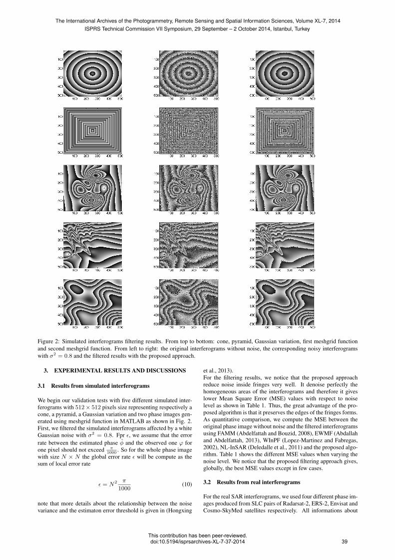
Figure 2: Simulated interferograms filtering results. From top to bottom: cone, pyramid, Gaussian variation, first meshgrid functionand second meshgrid function. From left to right: the original interferograms without noise, the corresponding noisy interferogramswith σ2 = 0.8 and the filtered results with the proposed approach.

3. EXPERIMENTAL RESULTS AND DISCUSSIONS

3.1 Results from simulated interferograms

We begin our validation tests with five different simulated inter-ferograms with 512× 512 pixels size representing respectively acone, a pyramid, a Gaussian variation and two phase images gen-erated using meshgrid function in MATLAB as shown in Fig. 2.First, we filtered the simulated interferograms affected by a whiteGaussian noise with σ2 = 0.8. Fpr ε, we assume that the errorrate between the estimated phase φ and the observed one ϕ forone pixel should not exceed π

1000. So for the whole phase image

with size N × N the global error rate ε will be compute as thesum of local error rate

ε = N2 π

1000(10)

note that more details about the relationship between the noisevariance and the estimaton error threshold is given in (Hongxing

et al., 2013).For the filtering results, we notice that the proposed approachreduce noise inside fringes very well. It denoise perfectly thehomogeneous areas of the interferograms and therefore it giveslower Mean Square Error (MSE) values with respect to noiselevel as shown in Table 1. Thus, the great advantage of the pro-posed algorithm is that it preserves the edges of the fringes forms.As quantitative comparison, we compute the MSE between theoriginal phase image without noise and the filtered interferogramsusing FAMM (Abdelfattah and Bouzid, 2008), EWMF (Abdallahand Abdelfattah, 2013), WInPF (Lopez-Martinez and Fabregas,2002), NL-InSAR (Deledalle et al., 2011) and the proposed algo-rithm. Table 1 shows the different MSE values when varying thenoise level. We notice that the proposed filtering approach gives,globally, the best MSE values except in few cases.

3.2 Results from real interferograms

For the real SAR interferograms, we used four different phase im-ages produced from SLC pairs of Radarsat-2, ERS-2, Envisat andCosmo-SkyMed satellites respectively. All informations about



Figure 3: Real interferograms filtering results. The first column using Radarsat-2 interferogram and the second column using ERSsatellite and from top to bottom: the original interferogram produced from ASTER DEM, the observed noisy interferogram, filteredwith the proposed approach and the filtering error with respect to column 1.

these four InSAR are available in (Ben Abdallah and Abdelfattah,2013). All tested real images are 512 × 512 pixels size. Similarto the simulated data, we consider the interferogram generatedby wrapping the Digital Elevation Model (DEM) provided byASTER Global DEM available in the Land Processes DistributedActive Archive Center website (Land Processes Distributed Ac-tive Archive Center, 2013) as the original interferogram withoutnoise. Note that since the four satellites, mentioned above, havingdifferent spatial resolutions, we should make under or over sam-pling to their InSARs to obtain the same resolution of ASTER’sinterferogram (30 × 30 meters). Next, we compare the filteringresults of the four InSARs with the reference one generated fromASTER’s DEM. In Fig. 3, we illustrate our estimation result andthe corresponding error map. For the statistical comparison, thesecond part of the Table 1 shows that the proposed approach giveslower error rate for the four real InSAR except in the case of ERSsatellite data.

4. CONCLUSION

The main idea of the interferometric phase filter proposed in thispaper is to smooth the homogeneous regions within the interfro-gram’s fringes. The low phase difference between pixels locatedin the same fringe of the interferogram leads to obtain a sparsesignal when we applying the gradient operator. This transformthe denoising problem to a l0 minimization problem which canbe solved using greedy algorithm. We used in this paper theApproximate Message Passing (AMP) algorithm. The proposedapproach is tested and validated on simulated and real interfero-grams and compared with two recent filters FAMM and EWMF.As future work, we will apply this approach to estimate the trueunwrapped phase value from the observed noisy interferogram.This will be done by twice applying the gradient operator and theLaplacien simultaneously.



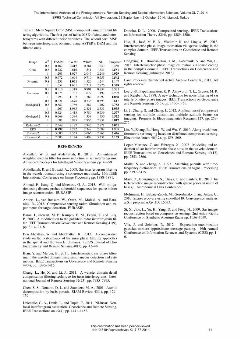
Table 1: Mean Square Error (MSE) computed using different fil-tering algorithms. The first part of table: MSE of simulated inter-ferograms with different noise variances. The second part: MSEbetween interferograms obtained using ASTER’s DEM and thefiltered ones.

Image σ2 FAMM EWMF WInPF NL Proposed0.5 0.462 0.417 0.781 1.249 0.450

Cone 0.8 0.722 0.616 1.541 1.334 0.5811 1.205 1.027 2.047 2.249 0.929

0.5 0.672 0.694 0.719 0.755 0.542Pyramid 0.8 1.233 1.031 1.520 1.244 1.147

1 1.654 1.651 2.214 2.876 1.5780.5 0.510 0.518 0.801 0.834 0.501

Gaussian 0.8 0.875 0.781 1.077 1.192 0.7571 1.293 1.102 1.789 2.097 1.068

0.5 0.621 0.575 0.738 0.593 0.617Meshgrid 1 0.8 0.887 0.789 1.387 1.702 0.783

1 1.267 1.083 2.831 2.333 1.0350.5 0.424 0.413 0.780 0.739 0.377

Meshgrid 2 0.8 0.669 0.594 1.339 1.330 0.5221 1.087 0.945 2.955 2.831 0.817

Radarsat-2 - 2.349 2.127 2.945 2.871 2.061ERS - 0.999 2.272 2.349 2.089 1.938

Envisat-2 - 3.000 2.553 3.066 2.967 2.476Cosmo-SM - 2.603 2.174 3.498 3.231 2.169

REFERENCES

Abdallah, W. B. and Abdelfattah, R., 2013. An enhancedweighted median filter for noise reduction in sar interferograms.Advanced Concepts for Intelligent Vision Systems pp. 49–59.

Abdelfattah, R. and Bouzid, A., 2008. Sar interferogram filteringin the wavelet domain using a coherence map mask. 15th IEEEInternational Conference on Image Processing pp. 1888–1891.

Ahmad, F., Jiang, Q. and Moeness, G. A., 2013. Wall mitiga-tion using discrete prolate spheroidal sequences for sparse indoorimage reconstruction. EURASIP.

Anitori, L., van Rossum, W., Otten, M., Maleki, A. and Bara-niuk, R., 2013. Compressive sensing radar: Simulation and ex-periments for target detection. EURASIP.

Baran, I., Stewart, M. P., Kampes, B. M., Perski, Z. and Lilly,P., 2003. A modification to the goldstein radar interferogram fil-ter. IEEE Transactions on Geoscience and Remote Sensing 41(9),pp. 2114–2118.

Ben Abdallah, W. and Abdelfattah, R., 2013. A comparativestudy on the performance of the insar phase filtering approchesin the spatial and the wavelet domains. ISPRS Journal of Pho-togrammetry and Remote Sensing 40(7), pp. 43–48.

Bian, Y. and Mercer, B., 2011. Interferometric sar phase filter-ing in the wavelet domain using simultaneous detection and esti-mation. IEEE Transactions on Geoscience and Remote Sensing49(4), pp. 1396–1416.

Chang, L., He, X. and Li, J., 2011. A wavelet domain detailcompensation filtering technique for insar interferograms. Inter-national Journal of Remote Sensing 32(23), pp. 7985–7995.

Chen, S. S., Donoho, D. L. and Saunders, M. A., 2001. Atomicdecomposition by basis pursuit. SIAM Review 43(1), pp. 129–159.

Deledalle, C.-A., Denis, L. and Tupin, F., 2011. Nl-insar: Non-local interferogram estimation. Geoscience and Remote Sensing,IEEE Transactions on 49(4), pp. 1441–1452.

Donoho, D. L., 2006. Compressed sensing. IEEE Transactionson Information Theory 52(4), pp. 1289–1306.

Hao, H., Jose, M. B.-D., Vladimir, K. and Lingda, W., 2013.Interferometric phase image estimation via sparse coding in thecomplex domain. IEEE Transactions on Geoscience and RemoteSensing.

Hongxing, H., Bioucas-Dias, J. M., Katkovnik, V. and Wu, L.,2013. Interferometric phase image estimation via sparse codingin the complex domain. IEEE Transactions on Geoscience andRemote Sensing (submitted 2013).

Land Processes Distributed Active Archive Center, h., 2013. Allrights reserved .

Lee, J.-S., Papathanassiou, K. P., Ainsworth, T. L., Grunes, M. R.and Reigber, A., 1998. A new technique for noise filtering of sarinterferometric phase images. IEEE Transactions on Geoscienceand Remote Sensing 36(5), pp. 1456–1465.

Li, J., Zhang, S. and Chang, J., 2012. Applications of compressedsensing for multiple transmitters multiple azimuth beams sarimaging. Progress In Electromagnetics Research 127, pp. 259–275.

Lin, Y., Zhang, B., Hong, W. and Wu, Y., 2010. Along-track inter-ferometric sar imaging based on distributed compressed sensing.Electronics letters 46(12), pp. 858–860.

Lopez-Martinez, C. and Fabregas, X., 2002. Modeling and re-duction of sar interferometric phase noise in the wavelet domain.IEEE Transactions on Geoscience and Remote Sensing 40(12),pp. 2553–2566.

Mallat, S. and Zhang, Z., 1993. Matching pursuits with time-frequency dictionaries. IEEE Transactions on Signal Processingpp. 3397–3415.

Mary, D., Bourguignon, S., Theys, C. and Lanteri, H., 2010. In-terferometric image reconstruction with sparse priors in union ofbases,”. Astronomical Data Conference.

Mohimani, H., Babaie-Zadeh, M., Gorodnitsky, I. and Jutten, C.,2010. Sparse recovery using smoothed l0: Convergence analysis.arXiv preprint arXiv:1001.5073.

Si, X., Jiao, L., Yu, H., Yang, D. and Feng, H., 2009. Sar imagesreconstruction based on compressive sensing. 2nd Asian-PacificConference on Synthetic Aperture Radar pp. 1056–1059.

Vila, J. and Schniter, P., 2012. Expectation-maximizationgaussian-mixture approximate message passing. 46th AnnualConference on Information Sciences and Systems (CISS) pp. 1–6.



new sar interferogram denoising method via sparse … · new sar interferogram denoising method via...

Documents