new reconstruction of antarctic near-surface...

New Reconstruction of Antarctic Near-Surface Temperatures: MultidecadalTrends and Reliability of Global Reanalyses*,+

JULIEN P. NICOLAS AND DAVID H. BROMWICH

Polar Meteorology Group, Byrd Polar Research Center, and Atmospheric Sciences Program, Department of

Geography, The Ohio State University, Columbus, Ohio

(Manuscript received 2 December 2013, in final form 21 July 2014)

ABSTRACT

A reconstruction of Antarctic monthly mean near-surface temperatures spanning 1958–2012 is presented.

Its primary goal is to take advantage of a recently revised key temperature record fromWestAntarctica (Byrd)

to shed further light on multidecadal temperature changes in this region. The spatial interpolation relies on

a kriging technique aided by spatiotemporal temperature covariances derived from three global reanalyses

[the European Centre for Medium-Range Weather Forecasts (ECMWF) Interim Re-Analysis (ERA-

Interim), Modern-Era Retrospective Analysis for Research and Applications (MERRA), and Climate

Forecast System Reanalysis (CFSR)]. For 1958–2012, the reconstruction yields statistically significant an-

nual warming in the Antarctic Peninsula and virtually all ofWest Antarctica, but no significant temperature

change in East Antarctica. Importantly, the warming is of comparable magnitude both in central West

Antarctica and in most of the peninsula, rather than concentrated either in one or the other region as

previous reconstructions have suggested. The TransantarcticMountains act for the temperature trends, as a

clear dividing line between East and West Antarctica, reflecting the topographic constraint on warm air ad-

vection from the Amundsen Sea basin. The reconstruction also serves to highlight spurious changes in the

1979–2009 time series of the three reanalyses that reduces the reliability of their trends, illustrating a long-

standing issue in high southern latitudes. The study concludes with an examination of the influence of the

southern annular mode (SAM) on Antarctic temperature trends. The results herein suggest that the trend of

the SAM toward its positive phase in austral summer and fall since the 1950s has had a statistically significant

cooling effect not only in East Antarctica (as already well documented) and but also (only in fall) in West

Antarctica.

1. Introduction

Long-term changes in Antarctic near-surface air tem-

perature constitute an important parameter affecting,

directly or indirectly, the Antarctic Ice Sheet’s mass

balance and its contribution to sea level rise. An increase

in temperature has two opposite effects for Antarctica.

The first effect is surface melting, which occurs when

the temperature approaches 08C. This can lead to mass

loss directly, through meltwater runoff, or indirectly, by

contributing to ice-shelf break-up, subsequent glacier

acceleration, and ultimately increasing ice discharge into

the ocean. The first mechanism (meltwater runoff), prom-

inent in Greenland, is still relatively limited in Antarctica

(Tedesco et al. 2007; Kuipers Munneke et al. 2012) and is

expected to remain largely so in the upcoming decades

(Krinner et al. 2007; Ligtenberg et al. 2013). The second

mechanism (ice-shelf weakening) is potentially far more

significant given the buttressing effect of the large coastal

ice shelves for the structurally unstableWest Antarctic Ice

Sheet (Joughin and Alley 2011). Melt ponding as a pre-

cursor of ice-shelf break-up has already been observed in

the Antarctic Peninsula (Rignot et al. 2004; Scambos et al.

2004; Pritchard and Vaughan 2007) but seems to have

played aminor role in the recent acceleration of glaciers in

the Amundsen Sea sector of West Antarctica, linked pri-

marily to warm ocean water and sub-ice-shelf melting

(Jacobs et al. 2011; Pritchard et al. 2012; Depoorter et al.

2013; Stanton et al. 2013).

*Byrd Polar Research Center Contribution Number 1445.1Supplemental information related to this paper is available at the

JournalsOnlinewebsite: http://dx.doi.org/10.1175/JCLI-D-13-00733.s1.

Corresponding author address: JulienNicolas,ByrdPolarResearch

Center, The Ohio State University, 1090 Carmack Rd., Columbus,

OH 43210.

E-mail: [email protected]

8070 JOURNAL OF CL IMATE VOLUME 27

DOI: 10.1175/JCLI-D-13-00733.1

� 2014 American Meteorological Society

http://dx.doi.org/10.1175/JCLI-D-13-00733.s1

mailto:[email protected]

The second effect of higher near-surface temperature

results from the positive exponential relationship be-

tween atmospheric moisture and temperature, and trans-

lates into greater snowfall over Antarctica and thus the

removal of water from the ocean. This phenomenon ac-

counts for the negative sea level contribution ofAntarctica

often projected for the twenty-first century (Gregory and

Huybrechts 2006; Bengtsson et al. 2011; Ligtenberg et al.

2013). However, the magnitude of the precipitation–

temperature sensitivity varies between studies and de-

pends in part on how well temperature changes near the

surface reflect those occurring aloft. Furthermore, recent

studies suggest that this future negative impact on sea level

may be offset by dynamical ice changes (Bindschadler

et al. 2013; Church et al. 2013), similar to what has

already been observed in recent years (Shepherd et al.

2012).

Given the large interannual and decadal variability

characteristic of Antarctic climate, placing recent

temperature changes in a longer-term context is im-

portant to determine their significance and the role of

natural variability versus anthropogenic forcing

(Schneider et al. 2006; Gillett et al. 2008; Goosse et al.

2012; Abram et al. 2013; Steig et al. 2013; Thomas et al.

2013). Data sparsity is the primary challenge that one

faces when trying to piece together the temperature

history of Antarctica. Direct meteorological observa-

tions in the region began for the most part with

the 1957–58 International Geophysical Year (IGY).

Poleward of 608S, a mere 15 research stations have

temperature records extending from the IGY (or im-

mediately thereafter) to the present. Despite their

small number, these records have been used to reveal

and investigate important aspects of Antarctic climate

change (e.g., Thompson and Solomon 2002; Vaughan

et al. 2003; Turner et al. 2005; Marshall et al. 2013;

Richard et al. 2013). The main limitation of these in-

vestigations is that 1) they rely on stations mostly lo-

cated on the coast, thus providing little insight into the

vast Antarctic interior, and 2) they largely leave aside

West Antarctica, owing to the lack of long-term con-

tinuous instrumental records in the region (here and

throughout the paper, West Antarctica is meant as

separate from the Antarctic Peninsula; see Fig. 1).

Global atmospheric reanalyses, which combine various

types of meteorological observations with the fields

from a weather forecasting model, represent a promis-

ing alternative for reconstructing the climate of Ant-

arctica from the past decades. Unfortunately, despite

significant progress made in recent reanalyses, their

trends have proven unreliable in high southern lati-

tudes (Hines et al. 2000; Marshall 2002; Bromwich and

Fogt 2004; Bromwich et al. 2007, 2011).

The spatial homogeneity of Antarctic monthly mean

temperature anomalies over hundreds of kilometers

(Comiso 2000; King and Comiso 2003) has fortunately

made it possible to exploit the sparse observation net-

work to reconstruct Antarctic temperatures from the

late 1950s onward. Since 2007, several temperature re-

constructions have been published, based on various

spatial interpolation techniques. The latter include nat-

ural neighbor interpolation modulated by a correlation

length scale parameter (Chapman and Walsh 2007), a

kriging-based method with a kriging field derived from

global reanalysis temperature data (Monaghan et al.

2008), and principal component analysis applied to sat-

ellite infrared skin temperature measurements (Steig

et al. 2009; O’Donnell et al. 2011). Some of these recon-

structions have been key in drawing attention to the

warming of West Antarctica since the IGY (Steig et al.

2009; Schneider et al. 2012a). However, differences in the

magnitude, pattern, and seasonality of this warming

among the reconstructions still undermine our current

understanding of the phenomenon.

These discrepancies can be attributed, in part, to dif-

ferent uses of the temperature observations from Byrd

(site 14 in Fig. 1). This dataset fills a vast data void be-

tween the western Ross Ice Shelf, South Pole, and the

northern Antarctic Peninsula, but it is unfortunately

only partially complete. Repeated efforts have been

made to fill in the temporal gaps of theByrd record using

various ancillary datasets (Shuman and Stearns 2001;

Reusch and Alley 2004; Monaghan et al. 2008; Küttelet al. 2012; Bromwich et al. 2013). The importance of the

Byrd record for Antarctic temperature reconstructions

is highlighted in Monaghan et al. (2008) by the marked

sensitivity of their results to the inclusion of Byrd in the

spatial interpolation. This comes from the fact that

temperature variability in central West Antarctica is

poorly captured by the surrounding long-term temper-

ature records (Bromwich et al. 2013), which in turn

stems from the distinct climatic nature of West Ant-

arctica compared to the rest of the continent (e.g., Guo

et al. 2004; Bromwich et al. 2004; Bindschadler 2006).

The infilling technique originally used by Monaghan

et al. (2008) was revised in 2010 to take advantage of

temperature data from automatic weather stations

closer to Byrd than the manned stations used originally

(Küttel et al. 2012). This revision had a significant impact

on the temperature trends reported for West Antarctica

(from insignificant cooling to highly significant warm-

ing), which were then in better agreement with those

found by Steig et al. (2009) (see Schneider et al. 2012a).

In an effort to ascertain long-term temperature changes

inWest Antarctica, Bromwich et al. (2013, 2014) recently

carried out a comprehensive reexamination of the Byrd

1 NOVEMBER 2014 N I COLAS AND BROMWICH 8071

temperature record from its start in 1957 to the present

time. This work resulted in more temporally consistent

observations and more reliable infilling of the data gaps.

Here, our purpose is to present the results from a new

reconstruction of Antarctic temperatures. The primary

motivations for adding a new dataset to those already

existing came from the importance of the Byrd record

mentioned above; the fact that none of the previous re-

constructions include its recent revisions; the current lack

of consensus on temperature changes inWest Antarctica;

and finally the multiple examples of ongoing rapid cli-

mate change in the very same region.

The paper is organized as follows. Data and methods

are described in section 2. The discussion of the results

(section 3) begins with an overview of the skill of our

reconstruction (section 3a), followed by a description of

the temperature variability and trends that can be in-

ferred from it (sections 3b–3e). The reconstruction is

then used to shed light on two issues: the reliability of

the temperature trends in global reanalyses (section 4a)

and the contribution of the southern annularmode (SAM)

to Antarctic temperature changes since the late 1950s

(section 4b). A summary and conclusions are given in

section 5. The following notation will be used hereafter to

refer to the three reconstructions most frequently cited:

S09 for Steig et al. (2009); M10 for the reconstruction of

Monaghan et al. (2008), revised in 2010; and O11 for

O’Donnell et al. (2011).

2. Data and method

a. Temperature datasets

A list of all the datasets used in this study along with

their reference(s) and website is given in Table 1. The

near-surface temperature records that are spatially in-

terpolated in our reconstruction come from 15Antarctic

stations and are available almost continuously from around

the IGY onward. The 15 stations are listed in Table 2 and

their locations are shown in Fig. 1. Their respective

monthly mean temperature time series are obtained from

theReferenceAntarcticData forEnvironmental Research

FIG. 1. Map of Antarctica showing the locations of the 15 stations used in the temperature

reconstruction (filled red circles). The station names and coordinates are listed in Table 2. The

thick green lines outline the boundaries of the three main Antarctic regions (boldface). Note

that, in this map and throughout the paper, West Antarctica does not include the Antarctic

Peninsula. The gray shades represent the topography from near sea level (darker gray) to

.4000m above mean sea level.


(READER) project (Turner et al. 2004), except for

Byrd, for which we used the reconstructed record from

Bromwich et al. (2013, 2014). For the few instances of

missing data in the 14 READER datasets, we use—

if they exist—the monthly temperature reports pub-

lished in the National Climatic Data Center’s Monthly

Climatic Data for the World (MCDW). The remainder

of the data gaps is treated as described at the end of

section 2b.

To determine the spatiotemporal covariances (kriging

fields) required in the spatial interpolation, we rely on

gridded monthly mean 2-m temperature (T2m) data

from three global reanalyses: the European Centre for

Medium-Range Weather Forecasts (ECMWF) Interim

Re-Analysis (ERA-Interim, herein ERAI; Dee et al.

2011); the National Aeronautic and Space Administration

(NASA) Modern-Era Retrospective Analysis for Re-

search andApplications (MERRA;Rienecker et al. 2011);

and the National Centers for Environmental Prediction

(NCEP) Climate Forecast System Reanalysis (CFSR;

Saha et al. 2010). When evaluated in high southern lat-

itudes, the three reanalyses have shown significantly

greater reliability than earlier-generation reanalyses

(Bromwich et al. 2011, 2013; Bracegirdle and Marshall

2012; Bracegirdle 2013; Screen and Simmonds 2012).

This improvement comes mainly as a result of improved

model physics, more advanced bias correction and data

assimilation techniques, and higher horizontal and ver-

tical model resolution.

For ERAI, we use two separate T2m datasets available

on the ECMWF data server: one originates from the

forecast fields (ERAI-f), the other from the analysis fields

(ERAI-a). The former is a product of 6-h model forecasts

and is interpolated from the reanalysis model lowest

vertical level. The latter is generated by the surface

analysis (Simmons et al. 2010; Dee et al. 2011)—a distinct

feature of ECMWF reanalyses—whereby screen-level

temperature observations are combined with the fore-

cast T2m field via optimal interpolation. This greater ob-

servational constraint, however, becomes a disadvantage

in our case as it is responsible for artifacts in the time

series caused by the changing availability of observations.

The three reanalyses range, in horizontal resolution,

from ;80 km for ERAI to ;55 km in MERRA to

;38 km in CFSR. For our purpose, they are bilinearly

interpolated to a common 60 3 60 km2 Cartesian grid.

They all start in January 1979 and, since their initial

release, have been updated up to themost recentmonths.

However, because access to themonthly data fromCFSR

is currently only possible through December 2009, we

restrict all reanalysis data to 1979–2009.

TABLE 1. List of datasets used in this study.

Dataset References Website

ERA-Interim Dee et al. (2011) data-portal.ecmwf.int/data/d/interim_full_moda/

MERRA Rienecker et al. (2011) disc.sci.gsfc.nasa.gov/daac-bin/DataHoldings.pl

CFSR Saha et al. (2010) rda.ucar.edu/datasets/ds093.2/

READER observations Turner et al. (2004) www.antarctica.ac.uk/met/READER/

MCDWa observations — www.ncdc.noaa.gov/IPS/mcdw/mcdw.html

Byrd temp record Bromwich et al. (2013, 2014) polarmet.osu.edu/Byrd_recon/

S09 temp reconstruction Steig et al. (2009) www.usap-data.org/entry/NSF-ANT04-40414/

2009-09-12_11-10-10/

M10 temp reconstructionb Monaghan et al. (2008), Küttel et al. (2012) Personal communication

O11 temp reconstructionc O’Donnell et al. (2011) www.climateaudit.info/data/odonnell/

SAM index Marshall (2003) www.antarctica.ac.uk/met/gjma/sam.html

a Monthly Climatic Data for the World.b This dataset refers to the reconstruction of Monaghan et al. (2008) subsequently revised in 2010.c A version of this dataset is also available, along with our temperature reconstructions, at polarmet.osu.edu/Antarctic_recon/.

TABLE 2. List of the 15 research stations whose temperature

records are used in our reconstruction. The numbers in the first

column refer to the locations shown in Fig. 1.

No. Station name Lat. Lon. Start

(8N) (8E) Year

1 Faraday/Vernadsky 265.2 264.3 1950

2 Esperanza* 263.4 257.0 1945

3 Orcadas 260.7 244.7 1903

4 Halley 275.6 226.6 1957

5 Novolazarevskaya 270.8 11.8 1961

6 Syowa 269.0 39.6 1957

7 Mawson 267.6 62.9 1954

8 Davis 268.6 78.0 1957

9 Mirny 266.6 93.0 1956

10 Vostok 278.5 106.8 1958

11 Casey 266.3 110.5 1959

12 Dumont d’Urville 266.7 140.0 1956

13 Scott Base 277.9 166.8 1957

14 Byrd 280.0 2119.5 1957

15 Amundsen-Scott 290.0 0.0 1957

* This station replaces Bellingshausen used by M10.


http://data-portal.ecmwf.int/data/d/interim_full_moda/

http://disc.sci.gsfc.nasa.gov/daac-bin/DataHoldings.pl

http://rda.ucar.edu/datasets/ds093.2/

http://www.antarctica.ac.uk/met/READER/

http://www.ncdc.noaa.gov/IPS/mcdw/mcdw.html

http://polarmet.osu.edu/Byrd_recon/

http://www.usap-data.org/entry/NSF-ANT04-40414/2009-09-12_11-10-10/

http://www.usap-data.org/entry/NSF-ANT04-40414/2009-09-12_11-10-10/

http://www.climateaudit.info/data/odonnell/

http://www.antarctica.ac.uk/met/gjma/sam.html

Wecompare our reconstructed temperatures with three

other Antarctic temperature reconstructions, namely the

M10 reconstruction; the main S09 reconstruction, based

on original (nondetrended) Advanced Very High Reso-

lution Radiometer (AVHRR) data; and the regularized-

least squares (RLS) reconstruction of O11.

b. Spatial interpolation method

Our reconstruction aims to produce estimates of

monthly mean temperature anomalies (i.e., departures

from the mean annual cycle) for all Antarctica from 1958

to 2012 based on the 15 station records mentioned above.

The interpolation method builds upon the kriging tech-

nique employed by M10 and originally developed to re-

constructAntarctic snowfall (Monaghan et al. 2006).Here,

we modify the original approach (primarily regarding the

definition of the kriging weights) to more fully exploit

some of the properties of ordinary kriging (Cressie 1993;

Olea 1999). A brief description of the two main equations

of the interpolation algorithm is provided below.

For a certain month t, the temperature anomaly Dypredicted at a certain location or grid point x is esti-

mated as the linear combination of the temperature

anomalies Dyk, k5 1, . . . , N, observed at the N stations

considered in the interpolation (here, N 5 15):

Dy(x, t)5 �N

k51

hk(x)lk(x)Dyk(t) . (1)

In this equation, lk(x) represents the weight ($0) as-

signed to the kth station at a certain location x on our

grid; hk(x) is either 1 or21 depending on the sign of the

temperature correlation between the kth station and

location x. To account for spatial differences in variance

(typically higher in the Antarctic interior and lower near

the coast), the temperature observations are normalized

by their respective standard deviations during 1979–

2009. Thus, Eq. (1) produces a normalized value, which

is then multiplied by the standard deviation of the re-

analysis data at location x to yield the final temperature

anomaly. The procedure is carried out separately for

each month and repeated with each reanalysis dataset.

The kriging weights (l) characterize the spatial rep-

resentativeness (or footprint) of the observations. These

footprints are determined from the T2m field of the four

global reanalyses mentioned above and defined as the

squared Pearson’s correlation coefficients (r2) between

the model temperature at the grid point closest to the

observations and the model temperature at every other

Antarctic grid point. The r2 coefficients are calculated

for 1979–2009 (our calibration period) from linearly

detrended reanalysis data. We denote r2k(x) the spatial

footprint associated with the kth observation.

One important aspect of kriging introduced here and

absent from M10 is the use of optimized weighting co-

efficients. In M10, the contributions of all observations

in the interpolation are considered, regardless of mul-

ticollinearity between some of the records and thus in-

creasing the risk of overfitting. This problem is

fortunately specifically addressed in ordinary kriging by

requiring the minimization of the estimation error

(Cressie 1993; Olea 1999). This condition is satisfied by

the following matrix equation defining the optimal

weights, noted l 5 (l1, . . . , lN)T:�

A 1

1T 0

�|fflfflfflfflfflffl{zfflfflfflfflfflffl}

A*

�l

a

�|ffl{zffl}l*

5

�b

1

�|ffl{zffl}b*

. (2)

Here, A is an N 3 N symmetric matrix describing the

covariances between observations; 1 is a column vector

of N ones; b is an N-element column vector containing

the spatial footprints evaluated at location x where the

temperature anomaly must be estimated; A*, l*, and b*

are identical to A, l, and b, respectively, except for one

additional element in each dimension; and the super-

script T denotes the transpose symbol. The elements of

A and b are defined as

Aij 5 r2i (xj) and bi 5 r2i (x) ,

with i 5 1, . . . , N and j 5 1, . . . , N (i and j are inter-

changeable with k used previously). The variable xj de-

notes the location (nearest grid point) of the jth

observation; a is a parameter known as the Lagrange

multiplier, required in the error minimization but without

further bearing on our method. Equation (2) can be

solved for l* (and therefore l) by inverting matrix A*.

This inversion yields weighting coefficients that are nor-

malized to one and can be supplied to Eq. (1) to predict

the temperature anomaly. A more detailed description of

the content of Eq. (2) is provided in appendix A.

One of the benefits of Eq. (2) is to handle the clus-

tering of observations, that is, to assign less overall weight

at nearby stations (e.g., along the coast of EastAntarctica)

than if these stations were considered in isolation, thereby

reducing the risk of overfitting. In addition, the values

predicted at the locations of the N input stations are

identical to the observations (kriging is an exact inter-

polation method; Lam 1983). A trade-off of having strong

observational anchor points is that our reconstruction in-

cludes a higher level of noise in the time series than those

based, for example, on mode decomposition, such as S09.

Our algorithm assumes complete temperature records

for all stations. A few of them, however, do contain data

gaps, even after infilling with MCDW monthly reports.


To reconstruct the temperature during the months when

missing data occur, we use a different set of l coefficients

calculated by omitting the stations (in most cases only

one station) with incomplete records. This approach

takes advantage of the large overlapping areas between

some of the stations’ spatial footprints.

c. Skill statistics

The combination of our interpolation algorithm with

the four reanalysis datasets produces four recon-

structions, referred to hereafter as RECONX, the sub-

script X standing for the reanalysis used to derive the

kriging weights. The respective skills of these recon-

structions are assessed through comparison against the

original reanalysis data and against observations from

Antarctic stations not used in the spatial interpolation

and obtained from READER (see the supplemental

material for the list of stations). These two comparisons

complement each other: reanalyses provide complete

spatial and temporal coverage but are subject to model

error and artifacts; observations, on the other hand, are

more reliable but are unevenly distributed in space and

time. We require a minimum of three complete years of

data for a record to be included in the evaluation and

exclude stations nearly collocatedwith others (in this case

keeping only the one with the longer record). Most of the

selected sites are concentrated in the northern Antarctic

Peninsula and western Ross Sea regions. Outside of the

peninsula, only three records extend back prior to 1980.

The four reconstructions are evaluated based on full-

reconstruction and verification statistics. Full-reconstruction

statistics evaluate the four ‘‘main’’ reconstructions (those

using 1979–2009 as calibration period) and exploit the

longest period during which both the validation dataset

(either observations or reanalysis) and the reconstruc-

tion are available simultaneously. Verification statistics

are derived from additional reconstructions produced

following the split calibration/verification approach

previously used in a number of climate reconstruction

studies (e.g., Cook et al. 1999; Mann and Rutherford

2002;Mann et al. 2005, 2008; S09) and implemented here

as follows: The 1979–2009 period is divided into two 15-yr

subperiods (1980–94 and 1995–2009). One subperiod is

used for calibration (i.e., to determine the kriging weights

and generate a new temperature reconstruction), while

the remainder of the 55 years (verification period) serves

for independent evaluation of the results. Each subperiod

is employed successively for calibration, yielding two sets

of statistics that are then averaged together.

The evaluation statistics include the Pearson’s co-

efficient of correlation (r), the root-mean-square error

(RMSE), the average explained variance (R2), and the

coefficient of efficiency (CE). Mathematical definitions

of R2 and CE can be found in appendix B (note the

difference between r2 and R2). The calculation of r and

R2 is based on linearly detrended time series, which in

effect reduces the impact of artificial trends present in

the reanalyses (cf. section 4a). No detrending is carried

out in the calculation of CE since one of the purposes of

this statistic is to determine the level of agreement be-

tween the mean values of the reconstruction and the

validation dataset (observations or reanalysis).

d. Uncertainty estimation

Our uncertainty estimation follows a similar approach

to the one employed by S09. We estimate the 95%

confidence interval around the reconstructed tempera-

tures as 62s, with s2 representing the total unresolved

variance of the reconstruction. The latter is calculated as

s2 5s2X(12CEX), where s

2X is the total variance of the

original temperature anomalies in reanalysisX, and (12CEX) is the fractional unresolved variance of the re-

construction relative to reanalysis X. To account for the

reconstruction error in the uncertainty of the tempera-

ture trends, we conduct (for each grid point) n 5 1000

Monte Carlo simulations whereby the temperature time

series are perturbed with Gaussian white noise having

a variance equal to s2. Trends are recomputed from the

n perturbed series and result in a trend distribution with

variance s2MC. This variance is then added to the squared

standard error of the regression coefficient (s2b) to pro-

duce an estimate of the total error of the trend:

sb0 5 (s2b 1s2

MC)1/2. The values of s2 and s2

MC are esti-

mated separately formonthly, seasonal, and annualmean

time series. The statistical significance of the trends is

based on a two-tailed t test. In this test, as well as in the

calculation of sb, the number of degrees of freedom is

adjusted for autocorrelations as in Santer et al. (2000).

Throughout the paper, the error bounds of the trends

represent the 95% confidence interval (i.e.,62sb0 for our

reconstruction and 62sb for other datasets).

e. SAM index and SAM-congruent trends

The SAM (also known as the Antarctic Oscillation) is

the dominant mode of atmospheric variability in the

extratropical Southern Hemisphere and describes the

near-zonally symmetric pattern of pressure–geopotential

height anomalies of opposite signs between mid and high

southern latitudes (Thompson and Wallace 2000). Our

analysis of the SAM–temperature relationships (section

4b) uses the SAM index fromMarshall (2003). This index

is defined as the standardized mean sea level pre-

ssure differences between 408 and 658S, based on obser-

vations from 12 stations roughly distributed along these

two latitudes. Several other SAM indices exist [see

Ho et al. (2012) for a review], some of which are


based on principal component analysis of the pressure–

geopotential height fields from global reanalyses, rather

than latitudinal pressure differences. Following the con-

clusions from Ho et al. (2012), we have elected to use the

Marshall SAM index for its reliability prior to 1979 (when

reanalyses are conversely less reliable) and thus for its

temporal consistency throughout the time span of our

reconstruction. One must keep in mind, however, that this

index emphasizes the zonally symmetric component of the

SAM,whereas its asymmetric component,most prominent

in austral winter and spring, is also known to have im-

portant climate impacts (Ding et al. 2012; Fogt et al. 2012).

We characterize the SAM–temperature relationships

via least squares linear correlations and regressions,

both performed on linearly detrended annual and sea-

sonal mean time series. The SAM contribution to Ant-

arctic temperature trends is estimated as in Thompson

et al. (2000) by calculating the temperature trends that

are linearly congruent with the SAM; that is, by first

linearly regressing Antarctic temperatures onto the

SAM index, and by then multiplying the resulting re-

gression coefficients by the trend in the SAM index. The

total error of the regression coefficient is quantified

following the same Monte Carlo procedure as the one

described above for the temperature trends (the SAM

index being used in place of the time axis). The relative

squared error of the SAM-congruent trend is then esti-

mated as the sum of the squared relative errors of the

SAM trend and the SAM–temperature regression co-

efficient, respectively. One important assumption be-

hind the use and interpretation of SAM-congruent trends

is that the SAM–temperature relationships observed on

an interannual basis (measured with detrended time se-

ries) remain valid on a multidecadal time scale (i.e., be-

tween the original, nondetrended time series).

3. Results

a. Evaluation of the temperature reconstructions

1) SUMMARY OF SKILL STATISTICS

Antarctic-averaged evaluation statistics based on

monthly temperature anomalies are presented in Table 3

and assess our four reconstructions with respect to

TABLE 3. Overall skill statistics for the four reconstructions presented in this study with respect to original reanalysis data and in-

dependent observations. The statistics shown are the root-mean-square error (RMSE), the correlation coefficient (r), the average ex-

plained variance (R2), and the coefficient of efficiency (CE). These statistics are based onmonthly temperature anomalies averaged across

all Antarctic grid points when compared to the reanalyses, and across all available observations otherwise (in this case, the number of

observations is indicated at the bottom of the column). The bottom part of the table shows performance statistics for the reanalyses

relative to observations. Boldface font highlights the dataset(s) with the highest skill for each parameter.

Full reconstructions

vs original reanalysis vs 1979–2012 observations vs 1958–78 observations

RMSE r R2 RMSE r R2 RMSE r R2

RECONERAI-a 1.34 0.83 0.69 1.36 0.80 0.61 1.59 0.69 0.24

RECONERAI-f 1.31 0.84 0.70 1.35 0.80 0.61 1.53 0.70 0.32

RECONMERRA 1.21 0.80 0.59 1.34 0.80 0.62 1.21 0.82 0.61

RECONCFSR 1.24 0.83 0.69 1.31 0.82 0.64 1.21 0.81 0.61No. of obs — — — 54 54 54 9 9 9

Verification reconstructions


RMSE r CE RMSE r CE RMSE r CE

RECONERAI-a 1.55 0.74 0.56 1.46 0.73 0.53 1.60 0.68 0.29

RECONERAI-f 1.52 0.75 0.57 1.45 0.73 0.53 1.54 0.69 0.36

RECONMERRA 1.37 0.72 0.44 1.40 0.76 0.57 1.26 0.79 0.59

RECONCFSR 1.44 0.75 0.57 1.41 0.74 0.56 1.25 0.79 0.60

No. of obs — — — 52 52 52 9 9 9

Reanalyses


RMSE r R2 RMSE r R2 RMSE r R2

ERAI-a — — — 1.07 0.88 0.69 — — —

ERAI-f — — — 1.03 0.89 0.73 — — —

MERRA — — — 1.27 0.84 0.65 — — —

CFSR — — — 1.11 0.88 0.73 — — —

No. of obs — — — 53 53 53 — — —


independent ground observations and original reanalysis

data. This table is adapted from Table 3 of O11 to facil-

itate comparison of the results. In their table, O11 assess

the skill of their own two reconstructions [RLS and

eigenvector-weighted (E-W)] and of the S09 recon-

struction relative to ground observations and toAVHRR

clear-sky skin temperature estimates. The results of our

Table 3 can be broken down as follows:

(i) The respective skills of our reconstructions are

overall comparable, regardless of the statistical

parameter or the dataset used for evaluation (re-

analysis or observations). The only exceptions are

the two ERAI-based reconstructions when evalu-

ated against pre-1979 observations. Their lower skill

can be mainly explained by poorer statistics in the

Antarctic Peninsula (wheremost of the few pre-1979

records are located), which in turn may be related to

the coarser resolution of ERAI compared to

MERRA and CFSR.

(ii) All statistics combined, RECONCFSR ranks first

among our four reconstructions. For this reason, it

is the one primarily used for the analysis presented

in the rest of the paper. Paradoxically, the temper-

ature trends in the original CFSR data are partic-

ularly unreliable over most of Antarctica (cf. Fig. 7,

discussed in section 4a). However, the detrending

of the reanalysis data prior to the calculation of the

kriging weights reduces the impact of this problem

on our reconstruction.

(iii) Comparison of the statistics shown in our Table 3

with those published in Table 3 ofO11 suggests that

our reconstructions have lower skill than the RLS

reconstruction of O11, have skill comparable to

their E-W reconstruction, and have higher skill

than S09. This comparison of statistics does have

certain limitations. First, the predictor (AVHRR or

reanalysis) and the number/locations of observations

differ between the reconstructions. Second, the two

methods used by O11 include calibration of

AVHRR principal components and spatial eigen-

vectors against all ground observations, hence a lack

of independence between reconstruction and obser-

vations; in contrast, these observations are fully

independent from our reconstructions. Third, the

statistics with respect to observations are averages

across all stations and thus tend to reflect the skill of

the reconstructions where the density of observa-

tions is greater (northern Antarctic Peninsula, west-

ern Ross Sea/Ross Ice Shelf).

(iv) The evaluation of the original reanalysis data

against observations (bottom of Table 3) reveals

substantially greater skill than AVHRR tempera-

tures, suggesting that the reanalyses provide amore

reliable predictor for the spatial interpolation. We

also note that the skill of ERAI-a (which assimi-

lates near-surface temperature observations) is

slightly lower than that of ERAI-f (which does

not), whereas one would expect the opposite. This

paradox can be explained by the spurious impact of

observations on ERAI-a time series.

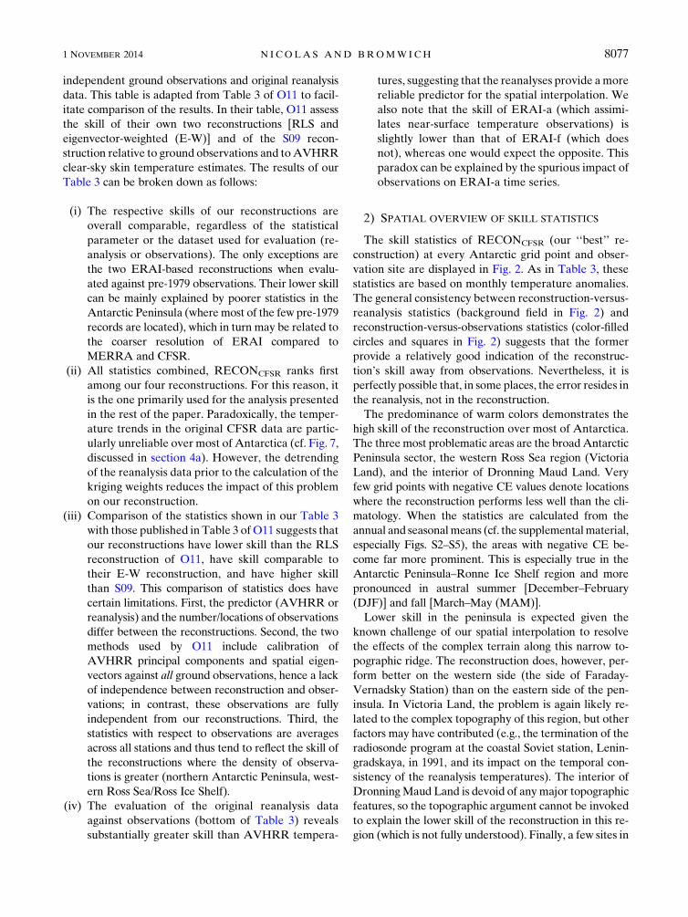
2) SPATIAL OVERVIEW OF SKILL STATISTICS

The skill statistics of RECONCFSR (our ‘‘best’’ re-

construction) at every Antarctic grid point and obser-

vation site are displayed in Fig. 2. As in Table 3, these

statistics are based on monthly temperature anomalies.

The general consistency between reconstruction-versus-

reanalysis statistics (background field in Fig. 2) and

reconstruction-versus-observations statistics (color-filled

circles and squares in Fig. 2) suggests that the former

provide a relatively good indication of the reconstruc-

tion’s skill away from observations. Nevertheless, it is

perfectly possible that, in some places, the error resides in

the reanalysis, not in the reconstruction.

The predominance of warm colors demonstrates the

high skill of the reconstruction over most of Antarctica.

The threemost problematic areas are the broadAntarctic

Peninsula sector, the western Ross Sea region (Victoria

Land), and the interior of Dronning Maud Land. Very

few grid points with negative CE values denote locations

where the reconstruction performs less well than the cli-

matology. When the statistics are calculated from the

annual and seasonalmeans (cf. the supplementalmaterial,

especially Figs. S2–S5), the areas with negative CE be-

come far more prominent. This is especially true in the

Antarctic Peninsula–Ronne Ice Shelf region and more

pronounced in austral summer [December–February

(DJF)] and fall [March–May (MAM)].

Lower skill in the peninsula is expected given the

known challenge of our spatial interpolation to resolve

the effects of the complex terrain along this narrow to-

pographic ridge. The reconstruction does, however, per-

form better on the western side (the side of Faraday-

Vernadsky Station) than on the eastern side of the pen-

insula. In Victoria Land, the problem is again likely re-

lated to the complex topography of this region, but other

factors may have contributed (e.g., the termination of the

radiosonde program at the coastal Soviet station, Lenin-

gradskaya, in 1991, and its impact on the temporal con-

sistency of the reanalysis temperatures). The interior of

DronningMaud Land is devoid of any major topographic

features, so the topographic argument cannot be invoked

to explain the lower skill of the reconstruction in this re-

gion (which is not fully understood). Finally, a few sites in


the East Antarctic interior indicate reduced skill of the

reconstruction locally. It is not certain whether the

problem can be traced to the difficulty of the reanalyses to

capture the strong temperature inversion that dominates

the temperature regime of the Antarctic boundary layer.

Fréville et al. (2014) recently showed, for example, that

this is a concern in ERAI and explains themarked surface

warm bias seen in this reanalysis. This issue has not yet

been investigated in other reanalyses.

b. Annual mean temperature time series

The annual mean temperature time series from

RECONCFSR spatially averaged over the three Ant-

arctic regions are shown in Fig. 3, along with sim-

ilar time series from the reconstructions of S09, M10,

and O11. In addition, Table 4 presents a quantitative

comparison of the four reconstructions, which in-

cludes detrended correlations with respect to our

FIG. 2. Skill statistics of RECONCFSR with respect to CFSR (background field) and independent observations (color-filled circles and

squares). The statistics are obtained by comparing, at each grid point, reconstructed and reanalysis or observed monthly temperature

anomalies. Full-reconstruction statistics are with respect to reanalysis data from 1979 to 2009 and all available observations. For verifi-

cation statistics, the comparison excludes reanalysis or observed data from the calibration period (see details in section 2d). Squares

denote stations with temperature records starting prior to 1979; circles are used otherwise. Blue shades denote areas where the re-

construction’s skill is lower than climatology.


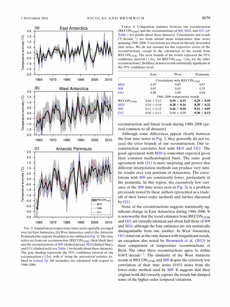
reconstruction and linear trends during 1960–2006 (pe-

riod common to all datasets).

Although some differences appear clearly between

the four time series in Fig. 3, they generally do not ex-

ceed the error bounds of our reconstruction. Our re-

construction correlates best with M10 and O11. The

good agreement with M10 is somewhat expected given

their common methodological basis. The same good

agreement with O11 is more surprising and proves that

different interpolation methods can produce very simi-

lar results over vast portions of Antarctica. The corre-

lations with S09 are consistently lower, particularly in

the peninsula. In this region, the excessively low vari-

ance of the S09 time series seen in Fig. 3c is a problem

previously noted by these authors (presented as a trade-

off of their lower-order method) and further discussed

by O11.

None of the reconstructions suggests statistically sig-

nificant change in East Antarctica during 1960–2006. It

is noteworthy that the trend estimates from RECONCFSR

andO11 are virtually identical and about half those of S09

and M10, although the four estimates are not statistically

distinguishable from one another. In West Antarctica,

O11 stand out as the only dataset with insignificant trends,

an exception also noted by Bromwich et al. (2013) in

their comparison of temperature reconstructions at

Byrd. The other three reconstructions agree to within

0.048Cdecade21. The similarity of the West Antarctic

trends in RECONCFSR and S09 despite the relatively low

correlation of their time series (0.65) arises from the

lower-order method used by S09. It suggests that their

original work did correctly capture the trends but damped

some of the higher-order temporal variations.

FIG. 3. Annual mean temperature times series spatially averaged

over (a) EastAntarctica, (b)WestAntarctica, and (c) theAntarctic

Peninsula (the regions’ boundaries are outlined in Fig. 1). The time

series are from our reconstruction (RECONCFSR; thick black line)

and the reconstructions of S09 (dashed green), M10 (dashed blue),

andO11 (dashed red) (see Table 1 for details about these datasets).

The gray shading represents the 95% confidence interval of our

reconstruction (62s), with s2 being the unresolved variance de-

fined in section 2d. All anomalies are calculated with respect to

1960–2006.

TABLE 4. Comparison statistics between our reconstruction

(RECONCFSR) and the reconstructions of S09, M10, and O11 (cf.

Table 1 for details about these datasets). Correlations and trends

(8Cdecade21) are from annual mean temperature time series

spanning 1960–2006. Correlations are based on linearly detrended

time series. We do not account for the respective errors of the

reconstructions, except in the calculation of the trends from

RECONCFSR. The error bounds of the trends represent the 95%

confidence interval (62sb0 for RECONCFSR, 62sb for the other

reconstructions). Boldface denotes trends statistically significant at

the 95% confidence level.

East West Peninsula

Correlations with RECONCFSR

M10 0.97 0.85 0.87

S09 0.81 0.65 0.53

O11 0.98 0.90 0.84

1960–2006 temperature trends

RECONCFSR 0.04 6 0.12 0.19 6 0.15 0.29 6 0.19M10 0.10 6 0.16 0.20 6 0.16 0.39 6 0.22

S09 0.11 6 0.12 0.16 6 0.10 0.11 6 0.07

O11 0.05 6 0.11 0.08 6 0.09 0.30 6 0.13


The trends from RECONCFSR for 1958–2012 (full ex-

tent of the reconstruction) are shown in Table 5. For the

annual temperature, the results are very similar to those

obtained for 1960–2006. The positive trend in East Ant-

arctica (0.06 6 0.098Cdecade21) remains statistically in-

significant. Our reconstruction suggests, however, that

2002–11 has been the warmest decade in East Antarctica

since 1958, coming after markedly colder 1990s. West

Antarctica and the Antarctic Peninsula exhibit sub-

stantially larger trends (0.22 6 0.128 and 0.33 60.178Cdecade21, respectively), as expected from the

mounting evidence of rapid warming of these two re-

gions (see the next section). Note that, for West Ant-

arctica, the magnitude and significance of the trend are

somewhat contingent upon the definition of the region’s

boundaries given the sharp contrast in temperature

change on either side of the Transantarctic Mountains

(cf. Fig. 4).

c. Temperature trend patterns during 1958–2012

The spatial distribution of the annual and seasonal

temperature trends derived from RECONCFSR for the

1958–2012 period are shown in Fig. 4. Kriging being an

exact interpolation method, the reconstruction’s trends

match very closely those observed at the 15 stations used in

the interpolation (cf. Fig. S6 in the supplementalmaterial).

The reconstruction reproduces the well-documented

rapid warming of the Antarctic Peninsula (Vaughan

et al. 2003; Turner et al. 2005). This is somewhat ex-

pected given the constraint provided by the two penin-

sula stations (Faraday-Vernadsky and Esperanza) used

in the spatial interpolation. This result is nonetheless

worth underscoring as the peninsula warming is not

equally captured by all reconstructions (see the previous

TABLE 5. Temperature trends (8Cdecade21) per Antarctic re-

gion during 1958–2012 (1959–2012 for DJF) from our re-

construction (RECONCFSR). ‘‘All’’ stands for all Antarctica. The

error bounds represent the 95% confidence interval (62sb0).

Boldface denotes trends statistically significant at this confidence

level.

Total temperature trends

All East West Peninsula

Annual 0.11 6 0.08 0.06 6 0.09 0.22 6 0.12 0.33 6 0.17

DJF 0.07 6 0.15 0.05 6 0.16 0.12 6 0.17 0.17 6 0.13MAM 0.01 6 0.18 20.03 6 0.20 0.08 6 0.21 0.32 6 0.21

JJA 0.16 6 0.20 0.09 6 0.23 0.28 6 0.27 0.58 6 0.36

SON 0.20 6 0.13 0.14 6 0.13 0.39 6 0.21 0.28 6 0.22

FIG. 4. Annual and seasonal mean temperature trends during 1958–2012 (1959–2012 for DJF) fromRECONCFSR. The thick solid black

line outlines areas with trends significant at the 95% confidence level when both the regression error and the reconstruction error are

accounted for. The thin dashed black line outlines the 95% significance contour when only the regression error is accounted for (i.e.,

assuming zero error in the reconstruction). For clarity, the notation NS highlights which side of the lines is not statistically significant.


section). In addition, the regional and seasonal charac-

teristics of this warming in the reconstruction are con-

sistent with those observed (Vaughan et al. 2003; Turner

et al. 2005; Marshall et al. 2006; van Lipzig et al. 2008),

with a maximum in austral winter [June–August (JJA)]

on the western side (although not clearly distinguishable

with the color scale) and a maximum in DJF on the

eastern side (in this case, statistically significant only at

the very northern tip of the peninsula). As a caveat, we

know from Fig. 2 that the reconstruction’s skill is overall

lower in the central and southern peninsula, meaning

that the trends in these regions must be interpreted with

caution. Yet, it is noteworthy that the strong warming

depicted in the southern portion of the peninsula is

consistent (at least qualitatively) with the warming seen

in the temperature proxy record from the Gomez ice

core (Thomas et al. 2009).

In the rest of the continent, the Transantarctic

Mountains largely act as a dividing line between West

Antarctic and East Antarctic temperature trends. Our

reconstruction shows significant warming in the annual

mean over most of West Antarctica, thereby confirming

evidence from borehole measurements (Barrett et al.

2009; Orsi et al. 2012), ice-core proxy records (Steig et al.

2013; Thomas et al. 2013), and—to various degrees—

other near-surface and tropospheric temperature re-

constructions (S09; O11; Schneider et al. 2012a; Screen

and Simmonds 2012). The seasonality and magnitude of

the trends in the central region largely reproduce those

described by Bromwich et al. (2013) for Byrd. The

strongest and most widespread warming occurs in aus-

tral spring [September–November (SON)], as high-

lighted by Schneider et al. (2012a). In JJA, most of West

Antarctica exhibits warming trends but statistical sig-

nificance is only reached in the eastern sector (facing the

Bellingshausen Sea). In DJF, there is suggestion of sig-

nificant warming over the Pine Island and Thwaites

Glaciers only when the reconstruction error is not ac-

counted for (cf. the method in section 2d). In other

words, the uncertainty of the reconstruction in this area

is currently too large to confirm this result. No significant

changes are seen in MAM, the season during which

West Antarctic temperatures have likely been most

impacted by the high-polarity SAM that has dominated

since the mid-1990s (cf. section 4b).

One further aspect of West Antarctic warming worth

highlighting is the tongue-shaped pattern assumed by

the trends across the central West Antarctic region. This

pattern is consistent with the atmospheric signature

typically associated with warm marine air intrusions

(Nicolas and Bromwich 2011a), thereby reflecting the

main atmospheric mechanism thought to be responsible

forWest Antarctic warming (Ding et al. 2011; Schneider

et al. 2012a; Bromwich et al. 2013). Note that the tongue

is not equally pronounced in our four reconstructions

and appears most clearly in RECONERAI-a and

RECONERAI-f (cf. Fig. S7 in the supplemental mate-

rial). On the one hand, the superiority of ERAI in

capturing the mean and transient atmospheric circula-

tion in the West Antarctic sector of the Southern Ocean

(Bracegirdle 2013) lends credence to the results of the

two ERAI-based reconstructions. On the other hand,

the reliability of this reanalysis is affected by clear evi-

dence of nonstationarity in its temperature over the

Ross Ice Shelf (cf. Fig. 8).

East Antarctica displays smaller regions of statisti-

cally significant trends. The largest patches of significant

warming occur in SON and are primarily concentrated

in the 908E–1808 quadrant. Cooling, on the other hand, ismore widespread in MAM and most pronounced at the

western (308W–08) and eastern (1208–1708E) edges of

East Antarctica. These regional coolings are likely re-

lated to atmospheric circulation changes that have pro-

moted offshore (cold) tropospheric flow over these areas

(Turner et al. 2009; Marshall et al. 2013). Other regional

features are also worth noting. For example, the tran-

sition from negative to positive trends near the Green-

wich meridian in the annual mean is consistent with the

temperature changes seen in several borehole records

from the area (Muto et al. 2011). The plateau-versus-

coast contrast in DJF is consistent with the more nega-

tive impact of a stronger SAM on temperatures in

coastal, katabatic-prone areas of Antarctica (Van den

Broeke and van Lipzig 2004). Finally, the more pro-

nounced warming in the 808–1008E sector is consistent

with the temperature signal seen in the coastal borehole

record analyzed by Roberts et al. (2013).

d. Comparison with trend patterns from otherreconstructions

Some similarities and differences between our re-

construction and those from S09, M10, and O11 have

already been pointed out above in the discussion of the

annual mean temperature time series (section 3b). The

comparison is extended here to the seasonal trend pat-

terns calculated for 1960–2006 (period common to all

datasets), shown in Fig. 5. Four points can be drawn

from this comparison:

1) InDJF, the strongwarmingpresent inM10over a large

fraction of West Antarctica is not found in any other

reconstruction. This can be explained by thewarmbias

initially present in the temperature observations from

Byrd and due to a calibration error. This bias has since

been corrected in the Byrd record investigated by

Bromwich et al. (2013) and used in our reconstruction.


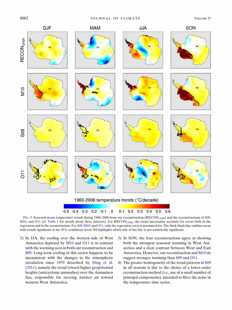
2) In JJA, the cooling over the western side of West

Antarctica depicted by M10 and O11 is in contrast

with the warming seen in both our reconstruction and

S09. Long-term cooling in this sector happens to be

inconsistent with the changes in the atmospheric

circulation since 1979 described by Ding et al.

(2011), namely the trend toward higher geopotential

heights (anticyclonic anomalies) over the Amundsen

Sea, responsible for steering warmer air toward

western West Antarctica.

3) In SON, the four reconstructions agree in showing

both the strongest seasonal warming in West Ant-

arctica and a clear contrast between West and East

Antarctica. However, our reconstruction andM10 do

suggest stronger warming than S09 and O11.

4) The greater homogeneity of the trend patterns in S09

in all seasons is due to the choice of a lower-order

reconstruction method (i.e., use of a small number of

principal components), intended to filter the noise in

the temperature time series.

FIG. 5. Seasonal mean temperature trends during 1960–2006 from our reconstruction (RECONCFSR) and the reconstructions of S09,

M10, and O11 (cf. Table 1 for details about these datasets). For RECONCFSR, the trend uncertainty accounts for errors both in the

regression and in the reconstruction. For S09, M10, andO11, only the regression error is accounted for. The thick black line outlines areas

with trends significant at the 95% confidence level; NS highlights which side of the line is not statistically significant.


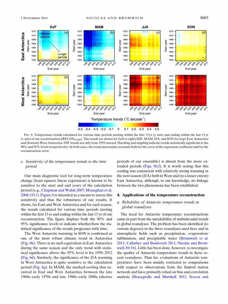
e. Sensitivity of the temperature trends to the timeperiod

Our main diagnostic tool for long-term temperature

change (least squares linear regression) is known to be

sensitive to the start and end years of the calculation

period (e.g., Chapman andWalsh 2007; Monaghan et al.

2008; O11). Figure 6 is intended as a means to assess this

sensitivity and thus the robustness of our results. It

shows, for East andWest Antarctica and for each season,

the trends calculated for various time periods starting

within the first 15 yr and ending within the last 15 yr of our

reconstruction. The figure displays both the 90% and

95% significance levels to indicate whether/how the sta-

tistical significance of the trends progresses with time.

The West Antarctic warming in SON is confirmed as

one of the most robust climate trend in Antarctica

(Fig. 6h). There is no such equivalent in East Antarctica

during the same season and the only trend with statis-

tical significance above the 95% level is for 1958–2012

(Fig. 6d). Similarly, the significance of the JJA warming

in West Antarctica is quite sensitive to the calculation

period (Fig. 6g). In MAM, the marked cooling that oc-

curred in East and West Antarctica between the late

1960s–early 1970s and late 1990s–early 2000s (shorter

periods of our ensemble) is absent from the more ex-

tended periods (Figs. 6b,f). It is worth noting that this

cooling was concurrent with relatively strong warming in

the next season (JJA) both inWest and (to a lesser extent)

East Antarctica, although, to our knowledge, no linkage

between the two phenomena has been established.

4. Applications of the temperature reconstruction

a. Reliability of Antarctic temperature trends inglobal reanalyses

The need for Antarctic temperature reconstructions

came in part from the unreliability of multidecadal trends

in global reanalyses. The problem has been identified (to

various degrees) in the three reanalyses used here and in

atmospheric fields such as precipitation, evaporation/

sublimation, and precipitable water (Bromwich et al.

2011; Cullather and Bosilovich 2011; Nicolas and Brom-

wich 2011b). Little has been done, however, to investigate

the quality of Antarctic temperature trends in these re-

cent reanalyses. Thus far, evaluations of Antarctic tem-

peratures have been mainly restricted to comparisons

with respect to observations from the limited station

network and have primarily relied on bias and correlation

analysis (Bracegirdle and Marshall 2012; Screen and

FIG. 6. Temperature trends calculated for various time periods starting within the first 15 yr (y axis) and ending within the last 15 yr

(x axis) of our reconstruction (RECONCFSR). The trends are shown for (left to right) DJF,MAM, JJA, and SON for (top) East Antarctica

and (bottom)WestAntarctica. DJF trends are only from 1959 onward. Hatching and stippling indicate trends statistically significant at the

90% and 95% levels (respectively). In both cases, the trend uncertainty accounts both for the error of the regression coefficient and for the

reconstruction error.


Simmonds 2012; Bromwich et al. 2013). One application

of our reconstructions is therefore to serve as a bench-

mark of reanalysis temperature trends over all Antarctica.

Figure 7 compares the trends in the annual mean

temperature from reconstructions and reanalyses during

1979–2009. The trend patterns from our four reconstruc-

tions bear very strong resemblance to each other, the small

differences being mostly confined to the peninsula. The

four reanalyses, on the other hand, reveal trend patterns

that are drastically different not only from those of the

reconstructions, but also from each other. In particular,

large values occur locally, often seen as a sign of spurious

changes in the time series. To help understand the origin of

these differences, the temperature anomalies for several

locations characterized by large trend values are plotted in

Fig. 8. Four conclusions can be drawn from Figs. 7 and 8:

1) The widespread warming seen in CFSR is mainly

explained by a shift in the temperature in the late

1990s (cf. the ‘‘AllAntarctica’’ plot in Fig. 8). This shift

is likely related to the beginning of the assimilation of

satellite radiances from the Advanced Television and

Infrared Observation Satellite (TIROS) Operational

Vertical Sounder (ATOVS) suite of instruments in

late 1998, already known to have had a global impact

on CFSR precipitation (Zhang et al. 2012). In com-

parison, none of the other reanalyses seems to have

a single dominant issue similar to theATOVSproblem

in CFSR.

2) ERAI exhibits considerably larger fluctuations in its

temperature than the two other reanalyses or our re-

construction. The fact that these fluctuations are seen

both in the analysis (ERAI-a) and the forecast (ERAI-f)

fields suggests that artifacts due to the assimilation of

near-surface temperature observations are likely not

the main cause of the problem. One notable excep-

tion is South Pole, where only ERAI-a diverges from

the other curves in the mid-1980s. Closer inspection

reveals that near-surface temperature observations

from this location, although available (since 1957),

were surprisingly not used in ERAI prior to 1985.

3) In some cases (other than South Pole), differences

between the reanalysis time series can be the result of

changes in a station’s location/elevation (which may

FIG. 7. Annual mean temperature trends during 1979–2009 based on (a)–(d) our four temperature reconstructions (the subscript

denotes the reanalysis used to derive the kriging field) and (e)–(h) the original T2m estimates from the four reanalysis datasets. The 95%

significance level of the trends is indicated as in Fig. 4.


or may not be taken into account by the reanalyses).

For example, in the vicinity of Casey (location 7 in

Fig. 8), the reanalyses start diverging in the late

1980s, that is, around the time of the opening of a new

station located 28m higher above sea level than the

previous facility (cf. Australian Bureau of Meteorol-

ogy, www.bom.gov.au/climate/data/). Similarly, in

coastal Dronning Maud Land (location 5 in Fig. 8),

the relocation of the South African station, South

African National Antarctic Expedition (SANAE),

from a coastal ice shelf to the top of a nunatak in the

late 1990s may explain the marked differences be-

tween the reanalyses. Further investigation would

certainly help confirm these hypotheses.

4) One advantage of our reconstructions is their tem-

poral consistency since, unlike the reanalyses, they

rely on a fixed network of observations. Although

greater consistency (clearly apparent in Fig. 8) can be

considered ‘‘more realistic,’’ it comes with a caveat: it

is not by itself proof that decadal temperature changes

are correctly captured by the reconstructions.

b. Influence of the SAM on Antarctic temperaturechange

The tendency for the SAM to stay in its high polarity

mode in austral summer and fall during recent decades is

considered the main atmospheric mechanism responsible

FIG. 8. Monthlymean temperature time series for variousAntarctic locations during 1979–2009 from our reconstruction (RECONCFSR;

black line) and from the original T2m data from the four reanalyses used this study (colored lines). The time series are shown as anomalies

with respect to the first five years (1979–1984) and are smoothed with a 36-month moving average. (top left) The first plot shows the

temperature anomalies spatially averaged over all Antarctica. The other plots show the temperature anomalies for the seven locations

displayed on the map in the bottom-right corner. The gray shading represents the 95% confidence interval of our reconstruction (62s),

with s2 being the unresolved variance (estimated separately for each location).


http://www.bom.gov.au/climate/data/

for modest temperature changes or cooling in East Ant-

arctica (Thompson and Solomon 2002; Turner et al. 2005;

Marshall 2007; Thompson et al. 2011). Note that the ac-

tual contribution of the SAM to the concurrent rapid

warming of the peninsula, particularly in the fall, is de-

bated (Ding and Steig 2013). In this section, we use our

reconstruction (RECONCFSR) to reexamine the SAM–

temperature relationships in Antarctica by expanding,

both spatially (particularly over West Antarctica) or tem-

porally, upon previous studies (e.g., Kwok and Comiso

2002; Thompson and Solomon 2002; Schneider et al. 2004,

2012a,b; Van den Broeke and van Lipzig 2004; Marshall

et al. 2006, 2013; Marshall 2007; Fogt et al. 2012). These

relationships are described by the correlation maps shown

in Fig. 9. The correlations are calculated only for 1958–

2012. As such, they do not capture the interdecadal

variability of the relationships seen in certain areas (see,

e.g., Marshall et al. 2011, 2013), and should therefore

only be regarded as the dominant characteristics during

this 55-yr period. Note that the correlation patterns are

very consistent across our four reconstructions (cf.

Fig. S8 in the supplemental material).

A high-polarity SAM (positive SAM index) is typi-

cally associated with lower temperatures in East Ant-

arctica. This cooling effect stems both from reduced

meridional heat exchange within the troposphere, and

from reduced downward turbulent heat flux near the ice

sheet’s surface (Van den Broeke and van Lipzig 2004).

The correlations are most negative in DJF within 500–

1000 km from the coast (the katabatic zone) and are

generally lower, yet still statistically significant, in SON.

The western edge of East Antarctica (08–408W) stands

out with insignificant correlations in all seasons but DJF.

This feature is consistent with the reversal of the sign of

the SAM–temperature relationship at Halley Station

(Marshall et al. 2011).

In the Antarctic Peninsula, the stronger circumpolar

flow associated with a positive SAM index enhances

warm air advection across the region, which in turn fa-

vors positive temperature anomalies, especially on the

eastern side (Marshall et al. 2006; van Lipzig et al. 2008).

However, Fig. 9 indicates that significant positive cor-

relations are restricted to the very northern tip of the

peninsula, and temperatures in the rest of the region are

positively correlated with the SAM only during MAM

and JJA, yet without statistical significance. This overall

lack of statistical significance can be explained by the

prominent influence of the tropics, especially El Niño–Southern Oscillation (ENSO), on atmospheric vari-

ability in and around the peninsula (Kwok and Comiso

FIG. 9. Pearson’s coefficient of correlation between the annual (or seasonal) mean temperatures from RECONCFSR at every grid point

in Antarctica and the annual (or seasonal) SAM index from Marshall (2003). The correlations are calculated for the 1958–2012 period

(1959–2012 for DJF) and are based on linearly detrended time series. The 95% significance level of the correlation is indicated as in Fig. 4.


2002; Schneider et al. 2012a; Ding and Steig 2013; Clem

and Fogt 2013). As mentioned above for the temperature

trends, one should keep inmind themore uncertain quality

of our reconstruction in the peninsula (especially in DJF

and MAM) when interpreting the correlation patterns.

In West Antarctica, the SAM–temperature correla-

tions are negative everywhere throughout the year

but—except in MAM—are small overall and not sta-

tistically significant. The contrast with respect to East

Antarctica can be traced, again, to a greater imprint of

ENSO in West Antarctica (e.g., Bromwich et al. 2000,

2004; Guo et al. 2004; Gregory and Noone 2008;

Schneider and Steig 2008; Okumura et al. 2012). On the

annual scale, the area of significant negative correlations

is roughly limited to the Ross Sea sector of West Ant-

arctica. This highlights the contrasting climate variabil-

ity between the eastern and western sides of West

Antarctica that is known from previous studies (e.g.,

Genthon et al. 2003; Kaspari et al. 2004).

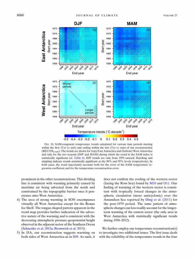
The overall contribution of SAM changes toAntarctic

temperature trends is estimated by calculating SAM-

congruent trends (Table 6). This contribution is only

apparent in the two seasons (DJF and MAM) during

which the SAM index exhibits statistically significant

(positive) trends since 1958. These trends have had

a statistically significant cooling effect in EastAntarctica

(in DJF and MAM) and West Antarctica (in MAM

only). By testing the sensitivity of the SAM-congruent

trends to the time period (Fig. 10), we find that the

SAM-related cooling is most robust in East Antarctica

in DJF, that it is consistently weak and insignificant in

West Antarctica in the same season, and that it is often

marginally significant both in East and West Antarctica

in MAM. Given that the temperature trends in DJF and

MAM are already positive or near zero (Table 5), it is

clear that the changes in the SAM in recent decades

have mitigated what could have been a stronger and

more significant Antarctic warming, as other studies

have suggested (Marshall 2007; Gillett et al. 2008;

Screen and Simmonds 2012).

5. Summary and conclusions

The temperature reconstruction presented in this

paper comes after several studies aiming to extend our

knowledge of temperature change over all Antarctica

back to the 1957–58 IGY by exploiting the information

from sparse long-term instrumental records (Chapman

and Walsh 2007; S09; M10; O11). Our own contribution

to this effort is primarily motivated by the recent release

of a new temperature record for Byrd, which happens to

be especially important for reconstructing past temper-

atures in West Antarctica. As in M10, our spatial in-

terpolation method uses a kriging framework aided by

spatiotemporal temperature covariances derived from

global reanalyses. The reanalysis data used here are taken

from four different T2m datasets: MERRA, CFSR, ERAI

analysis, and ERAI forecast. Four reconstructions are

generated as a result. Our evaluation finds higher skill in

the CFSR-based reconstruction (RECONCFSR), which is

the one whose results are primarily shown and discussed

throughout the paper. Our main findings can be summa-

rized as follows:

1) The reconstructed temperature time series spatially

averaged over the three Antarctic regions show

statistically significant warming throughout the year

in the Antarctic Peninsula, in SON and JJA in West

Antarctica, and in SON in East Antarctica during the

1958–2012 period. While the West Antarctic warm-

ing in SON is quite robust to the calculation period, it

is less so for the two other trends.

2) The annual warming is of similar magnitude both in

centralWest Antarctica and in most of the peninsula,

rather than concentrated either in the former (as in

S09) or in the latter (as in O11). However, the

seasonality and spatial patterns of the trends suggest

different origins to the warming in these two regions.

3) A sharp contrast appears in the temperature trend

maps on either sides of the Transantarctic Moun-

tains, particularly in JJA and SON. The same con-

trast is also seen in the results from S09 but is less

TABLE 6. Trends in the annual and seasonal SAM index from Marshall (2003) and SAM-congruent temperature trends (8Cdecade21)

per Antarctic region during 1958–2012 (1959–2012 for DJF). ‘‘All’’ stands for all Antarctica. SAM index trends are in units of standard

deviation per decade (the standard deviation is calculated for 1958–2012). The error bounds of the trends represent the 95% confidence

interval (62sb for SAM index trends,62sb0 for SAM-congruent trends). Boldface denotes trends statistically significant at this confidence

level.

Trends in SAM index

SAM-congruent temperature trends

All East West Peninsula

Annual 0.27 6 0.16 20.08 6 0.06 20.09 6 0.07 20.07 6 0.07 0.03 6 0.09

DJF 0.23 6 0.18 20.10 6 0.09 20.11 6 0.10 20.07 6 0.08 20.01 6 0.05

MAM 0.24 6 0.19 20.16 6 0.13 20.18 6 0.15 20.15 6 0.14 0.06 6 0.10

JJA 0.12 6 0.19 20.08 6 0.13 20.10 6 0.16 20.06 6 0.10 0.05 6 0.10

SON 20.01 6 0.20 0.00 6 0.08 0.00 6 0.08 0.00 6 0.07 0.00 6 0.01


prominent in the other reconstructions. This dividing

line is consistent with warming primarily caused by

maritime air being advected from the north and

constrained by the topographic barrier once it pen-

etrates onto West Antarctica.

4) The area of strong warming in SON encompasses

virtually all West Antarctica except for the Ronne

Ice Shelf. The tongue-shaped pattern apparent in the

trend map provides further indication of the advec-

tive nature of the warming and is consistent with the

decreasing atmospheric pressure–geopotential height

observed in the adjacent sector of the Southern Ocean

(Schneider et al. 2012a; Bromwich et al. 2013).

5) In JJA, our reconstruction suggests warming on

both sides of West Antarctica as in S09. As such, it

does not confirm the cooling of the western sector

(facing the Ross Sea) found by M10 and O11. Our

finding of warming of the western sector is consis-

tent with tropically forced changes in the atmo-

spheric circulation (more anticyclonic) over the

Amundsen Sea reported by Ding et al. (2011) for

the post-1979 period. The same pattern of atmo-

spheric changes can less readily account for the longer-

term warming of the eastern sector (the only area in

West Antarctica with statistically significant trends

during 1958–2012).

We further employ our temperature reconstruction(s)

to investigate two additional issues. The first issue deals

with the reliability of the temperature trends in the four

FIG. 10. SAM-congruent temperature trends calculated for various time periods starting

within the first 15 yr (y axis) and ending within the last 15 yr (x axis) of our reconstruction

(RECONCFSR). The trends are shown for (top) East Antarctica and (bottom)West Antarctica

and only for the two seasons (DJF and MAM) during which the trend in the SAM index is

statistically significant (cf. Table 6). DJF trends are only from 1959 onward. Hatching and

stippling indicate trends statistically significant at the 90% and 95% levels (respectively). In

both cases, the trend uncertainty accounts both for the error of the SAM–temperature re-

gression coefficient and for the temperature reconstruction error.


reanalysis datasets used to derive the temperature co-

variances. Our analysis highlights spurious temperature

changes in various parts of Antarctica in each reanalysis,

with varying characteristics. For example, the impact of

the assimilation of ATOVS data is clearly seen in CFSR

in the late 1990s. Large temperature shifts in ERAI cast

doubt on its reliability but do not seem tied to a single

problem. These artifacts in the time series represent one

important source of error in our reconstruction, al-

though their impact can be reduced by linearly

detrending the reanalysis data. Beyond the scope of our

reconstruction, and given the prominent role of global

reanalyses in shaping our understanding of Antarctic

climate change in recent decades, it would be desirable

to understand the origin of these problems in order to

avoid their reappearance in future reanalyses.

The second issue is the characterization of the in-

fluence of the SAM on Antarctic temperatures during

the 1958–2012 period. Our analysis largely confirms the

spatial pattern of the SAM–temperature relationship

described in previous studies but provides additional

insight on this relationship in West Antarctica. We

show, via the calculation of SAM-congruent tempera-

ture trends, that the positive trend in the SAM index in

recent decades has had a statistically significant cooling

effect in East Antarctica in DJF and MAM and in West

Antarctica in MAM. This SAM-related cooling may be

interpreted as the additional warming thatmight occur if

the SAM were to revert to its average pre-1980 (‘‘pre–

ozone hole’’) state. Future weakening of the SAM may

result, for example, from the Antarctic ozone recovery

projected for the rest of the twenty-first century, but

many sources of uncertainty remain regarding this sce-

nario, pertaining to current climate model projections

(Perlwitz et al. 2008; Zheng et al. 2013), to the role of

natural variability in SAM changes (Marshall et al.

2004), or to interactions between SAMand ENSO (Fogt

et al. 2011). The uncertain nature of the relationship

between SAM and Antarctic temperatures (Bitz and

Polvani 2012;Marshall et al. 2013) is another item to add

to the list. Until reanalysis data in Antarctica can extend

reliably back to the IGY (or beyond), temperature re-

constructions will likely remain an important tool to

investigate this issue.

Acknowledgments. This research was supported by

NASA Grant NN12AI29G and by National Science

Foundation Grants PLR-1049089 and PLR-1341695.

We thank Andrew Monaghan for his temperature re-

construction data and for his insight at various stages of

this work. We are also grateful to three anonymous re-

viewers for their comments, which helped improve the

paper.

APPENDIX A

Optimal Kriging Weights

This appendix details the content of Eq. (2) used to

determine the weights of the observations in the spatial

interpolation. Using the same notation as in section 2b,

we define the following variables and parameters of the

equation (with i 5 1, . . . , N and j 5 1, . . . , N):

d N, the number of observations;d xi, the location (nearest grid point) of the ith

observation;d x, the location (grid point) where the temperature

anomaly must be estimated;d r2i (xj), the squared Pearson’s correlation between the

model temperature at the grid point closest to the ith

observation and the model temperature at the grid

point closest to the jth observation [note that

r2i (xj)5 r2j (xi)];d r2i (x), the squared Pearson’s correlation between the

model temperature at the grid point closest to the ith

observation and the model temperature at a certain

location (grid point) x;d a, a parameter known as the Lagrange multiplier; andd li, the weight assigned to the ith observation (i.e., the

unknown).

The theory of ordinary kriging (e.g., Cressie 1993;

Olea 1999) dictates that the weighting coefficients li are

optimal if they minimize the estimation error (kriging

variance). This condition requires the coefficients to

be solutions of the following system of N 1 1 linear

equations:

8>>>>>>>>>>>>>>><>>>>>>>>>>>>>>>:

�N

i51

lir21(xi)1a5 r21(x)

�N

i51

lir22(xi)1a5 r22(x)

. . . . . .

�N

i51

lir2N(xi)1a5 r2N(x)

�N

i51

li5 1

In matrix notation, the system becomes

266664r21(x1) . . . r21(xN) 1

..

.⋱ ..

.1

r2N(x1) . . . r2N(xN) 1

1 1 1 0

377775

|fflfflfflfflfflfflfflfflfflfflfflfflfflfflfflfflfflfflfflfflfflfflfflfflfflffl{zfflfflfflfflfflfflfflfflfflfflfflfflfflfflfflfflfflfflfflfflfflfflfflfflfflffl}A*

266664

l1

..

.

lNa

377775

|fflfflffl{zfflfflffl}l*

5

266664r21(x)

..

.

r2N(x)

1

377775

|fflfflfflfflfflffl{zfflfflfflfflfflffl}b*


APPENDIX B

Definition of Statistical Parameters

Our evaluation statistics include the average explained

variance (R2, the coefficient of determination) during

the ‘‘full reconstruction period’’ (i.e., the longest period

of overlap between reconstruction and observations–

reanalyses), and the coefficient of efficiency (CE) during

the calibration period. The two statistics are defined as in

Cook et al. (1994, 1999), the only difference being that

these authors restrict the calculation of R2 to their cali-

bration period whereas the full reconstruction period is

used here (as in O11).

The R2 coefficient is calculated as follows:

R25 1:02�(yt 2 yt)

2

�(yt 2 yFR)2,

where yt are the temperature anomalies from the vali-

dation data (observations or reanalysis), yt are the

temperature anomalies from our reconstruction, and t is

a point in time (month, season, or year) during the full

reconstruction period; yFR is the mean of yt during the

same period. The CE statistic is calculated in a very

similar fashion:

CE5 1:02�(yt 2 yt)

2

�(yt 2 yy)2.

In this case, yt, yt, and yy are all restricted to the verifi-

cation period. The reference period for all anomalies is

the full reconstruction period. It follows that, in our

particular case, yFR 5 0 and (in general) yy 6¼ 0.

The R2 and CE statistics compare the error of the

reconstruction to the error arising from simply using the

climatological mean. They range from 2‘ to 11, with

positive values indicating greater skill than climatology

(our goal here). Note that R2 differs from the squared

Pearson’s correlation coefficient, r2. Both would be

equivalent if y were based on a simple univariate least

squares linear regression of y (Ott 1993), which is not the

case here. Unlike r2, R2 can take on negative values (cf.

Fig. S2 in the supplemental material). In those instances,

the problem may reside in the reanalysis data rather

than the reconstruction. Further details about theR2 and

CE statistics can be found in Cook et al. (1994, 1999).

REFERENCES

Abram,N. J., andCoauthors, 2013: Acceleration of snowmelt in an

Antarctic Peninsula ice core during the twentieth century.Nat.

Geosci., 6, 404–411, doi:10.1038/ngeo1787.

Barrett, B. E., K. W. Nicholls, T. Murray, A. M. Smith, and D. G.

Vaughan, 2009: Rapid recent warming on Rutford Ice Stream,

West Antarctica, from borehole thermometry. Geophys. Res.

Lett., 36, L02708, doi:10.1029/2008GL036369.

Bengtsson, L., S. Koumoutsaris, and K. Hodges, 2011: Large-scale

surface mass balance of ice sheets from a comprehensive at-

mospheric model. Surv. Geophys., 32, 459–474, doi:10.1007/

s10712-011-9120-8.

Bindschadler, R., 2006: The environment and evolution of theWest

Antarctic ice sheet: Setting the stage. Philos. Trans. Roy. Soc.,

364A, 1583–1605, doi:10.1098/rsta.2006.1790.

——, and Coauthors, 2013: Ice-sheet model sensitivities to envi-

ronmental forcing and their use in projecting future sea level

(the SeaRISE project). J. Glaciol., 59, 195–224, doi:10.3189/

2013JoG12J125.

Bitz, C. M., and L. M. Polvani, 2012: Antarctic climate response to

stratospheric ozone depletion in a fine resolution ocean cli-

mate model. Geophys. Res. Lett., 39, L20705, doi:10.1029/

2012GL053393.

Bracegirdle, T. J., 2013: Climatology and recent increase of west-

erly winds over the Amundsen Sea derived from six re-

analyses. Int. J. Climatol., 33, 843–851, doi:10.1002/joc.3473.

——, and G. J. Marshall, 2012: The reliability of Antarctic tropo-

spheric pressure and temperature in the latest global reanalyses.

J. Climate, 25, 7138–7146, doi:10.1175/JCLI-D-11-00685.1.

Bromwich, D. H., and R. L. Fogt, 2004: Strong trends in the skill of

the ERA-40 and NCEP–NCAR reanalyses in the high and

middle latitudes of the Southern Hemisphere, 1958–2001. J. Cli-

mate, 17, 4603–4619, doi:10.1175/3241.1.

——,A. N. Rogers, P. Kållberg, R. I. Cullather, J.W. C.White, and

K. J. Kreutz, 2000: ECMWF analyses and reanalyses depic-

tion of ENSO signal in Antarctic precipitation. J. Climate,

13, 1406–1420, doi:10.1175/1520-0442(2000)013,1406:

EAARDO.2.0.CO;2.

——, A. J. Monaghan, and Z. Guo, 2004: Modeling the ENSO

modulation ofAntarctic climate in the late 1990swithPolarMM5.

J. Climate, 17, 109–132, doi:10.1175/1520-0442(2004)017,0109:

MTEMOA.2.0.CO;2.

——, R. L. Fogt, K. I. Hodges, and J. E. Walsh, 2007: A tropo-

spheric assessment of the ERA-40, NCEP, and JRA-25 global

reanalyses in the polar regions. J. Geophys. Res., 112,D10111,

doi:10.1029/2006JD007859.

——, J. P. Nicolas, and A. J. Monaghan, 2011: An assessment of

changes in Antarctic and Southern Ocean precipitation since

1989 in contemporary global reanalyses. J. Climate, 24, 4189–

4209, doi:10.1175/2011JCLI4074.1.

——, ——, ——, M. A. Lazzara, L. M. Keller, G. A. Weidner, and

A. B. Wilson, 2013: Central West Antarctica among the most

rapidly warming regions on Earth. Nat. Geosci., 6, 139–145,

doi:10.1038/ngeo1671.

——, ——, ——, ——, ——, ——, and ——, 2014: Corrigendum:

Central West Antarctica among the most rapidly warming

regions on Earth. Nat. Geosci., 7, 76, doi:10.1038/ngeo2016.

Chapman, W. L., and J. E. Walsh, 2007: A synthesis of Antarctic

temperatures. J. Climate, 20, 4096–4117, doi:10.1175/JCLI4236.1.

Church, J., and Coauthors, 2013: Sea level change.Climate Change

2013: The Physical Science Basis. T. Stocker et al., Eds.,

Cambridge University Press, 1137–1216.

Clem, K. R., and R. L. Fogt, 2013: Varying roles of ENSO and SAM

on theAntarctic Peninsula climate in austral spring. J. Geophys.

Res. Atmos., 118, 11481–11492, doi:10.1002/jgrd.50860.Comiso, J. C., 2000: Variability and trends in Antarctic surface

temperatures from in situ and satellite infrared measurements.


http://dx.doi.org/10.1038/ngeo1787

http://dx.doi.org/10.1029/2008GL036369

http://dx.doi.org/10.1007/s10712-011-9120-8

http://dx.doi.org/10.1007/s10712-011-9120-8

http://dx.doi.org/10.1098/rsta.2006.1790

http://dx.doi.org/10.3189/2013JoG12J125

http://dx.doi.org/10.3189/2013JoG12J125

http://dx.doi.org/10.1029/2012GL053393

http://dx.doi.org/10.1029/2012GL053393

http://dx.doi.org/10.1002/joc.3473

http://dx.doi.org/10.1175/JCLI-D-11-00685.1

http://dx.doi.org/10.1175/3241.1

http://dx.doi.org/10.1175/1520-0442(2000)013<1406:EAARDO>2.0.CO;2

http://dx.doi.org/10.1175/1520-0442(2000)013<1406:EAARDO>2.0.CO;2

http://dx.doi.org/10.1175/1520-0442(2004)017<0109:MTEMOA>2.0.CO;2

http://dx.doi.org/10.1175/1520-0442(2004)017<0109:MTEMOA>2.0.CO;2

http://dx.doi.org/10.1029/2006JD007859

http://dx.doi.org/10.1175/2011JCLI4074.1



http://dx.doi.org/10.1175/JCLI4236.1

http://dx.doi.org/10.1002/jgrd.50860

J. Climate, 13, 1674–1696, doi:10.1175/1520-0442(2000)013,1674:

VATIAS.2.0.CO;2.

Cook, E. R., K. R. Briffa, and P. D. Jones, 1994: Spatial regression

methods in dendroclimatology: A review and comparison of

two techniques. Int. J. Climatol., 14, 379–402, doi:10.1002/

joc.3370140404.

——, D. M. Meko, D. W. Stahle, and M. K. Cleaveland, 1999:

Drought reconstructions for the continental United States.

J. Climate, 12, 1145–1162, doi:10.1175/1520-0442(1999)012,1145:

DRFTCU.2.0.CO;2.

Cressie, N. A., 1993: Statistics for Spatial Data. Wiley, 900 pp.

Cullather, R. I., and M. G. Bosilovich, 2011: The moisture budget

of the polar atmosphere in MERRA. J. Climate, 24, 2861–

2879, doi:10.1175/2010JCLI4090.1.

Dee, D. P., and Coauthors, 2011: The ERA-Interim reanalysis:

Configuration and performance of the data assimilation sys-

tem. Quart. J. Roy. Meteor. Soc., 137, 553–597, doi:10.1002/

qj.828.

Depoorter, M. A., J. L. Bamber, J. A. Griggs, J. T. M. Lenaerts,

S. R. M. Ligtenberg, M. R. van den Broeke, and G. Moholdt,

2013: Calving fluxes and basal melt rates of Antarctic ice

shelves. Nature, 502, 89–92, doi:10.1038/nature12567.

Ding, Q., and E. J. Steig, 2013: Temperature change on the Ant-

arctic Peninsula linked to the tropical Pacific. J. Climate, 26,

7570–7585, doi:10.1175/JCLI-D-12-00729.1.

——, ——, D. S. Battisti, and M. Küttel, 2011: Winter warming in

West Antarctica caused by central tropical Pacific warming.

Nat. Geosci., 4, 398–403, doi:10.1038/ngeo1129.

——, ——, ——, and J. M. Wallace, 2012: Influence of the tropics

on the southern annular mode. J. Climate, 25, 6330–6348,

doi:10.1175/JCLI-D-11-00523.1.

Fogt, R. L., D. H. Bromwich, and K. M. Hines, 2011: Un-

derstanding the SAM influence on the South Pacific ENSO

teleconnection. Climate Dyn., 36, 1555–1576, doi:10.1007/

s00382-010-0905-0.

——, J. M. Jones, and J. Renwick, 2012: Seasonal zonal asymme-

tries in the southern annular mode and their impact on re-

gional temperature anomalies. J. Climate, 25, 6253–6270,

doi:10.1175/JCLI-D-11-00474.1.

Fréville, H., E. Brun, G. Picard, N. Tatarinova, L. Arnaud,

C. Lanconelli, C. Reijmer, and M. van den Broeke, 2014:

UsingMODIS land surface temperatures and the Crocus snow

model to understand the warm bias of ERA-Interim re-

analyses at the surface in Antarctica. Cryosphere Discuss., 8,

55–84, doi:10.5194/tcd-8-55-2014.

Genthon, C., G. Krinner, and M. Sacchettini, 2003: Interannual

Antarctic tropospheric circulation and precipitation variabil-

ity. Climate Dyn., 21, 289–307, doi:10.1007/s00382-003-0329-1.

Gillett, N. P., D. A. Stone, P. A. Stott, T. Nozawa, A. Y. Karpechko,

G. C. Hegerl, M. F. Wehner, and P. D. Jones, 2008: Attribution

of polar warming to human influence. Nat. Geosci., 1, 750–754,

doi:10.1038/ngeo338.

Goosse, H., and Coauthors, 2012: Antarctic temperature changes

during the last millennium: Evaluation of simulations and

reconstructions. Quat. Sci. Rev., 55, 75–90, doi:10.1016/

j.quascirev.2012.09.003.

Gregory, J., and P. Huybrechts, 2006: Ice-sheet contributions

to future sea-level change. Philos. Trans. Roy. Soc., A364,

1709–1732.

Gregory, S., and D. Noone, 2008: Variability in the teleconnection

between the El Niño–Southern Oscillation and West Antarctic

climate deduced from West Antarctic ice core isotope records.

J. Geophys. Res., 113, D17110, doi:10.1029/2007JD009107.

Guo, Z., D. H. Bromwich, and K. Hines, 2004: Modeled Antarctic

precipitation. Part II: ENSO modulation over West Antarctica.

J. Climate, 17, 448–465, doi:10.1175/1520-0442(2004)017,0448:

MAPPIE.2.0.CO;2.

Hines, K. M., D. H. Bromwich, and G. J. Marshall, 2000: Artificial

surface pressure trends in the NCEP–NCAR reanalysis over

the SouthernOcean andAntarctica. J. Climate, 13, 3940–3952,

doi:10.1175/1520-0442(2000)013,3940:ASPTIT.2.0.CO;2.

Ho, M., A. S. Kiem, and D. C. Verdon-Kidd, 2012: The southern

annular mode: A comparison of indices. Hydrol. Earth Syst.

Sci., 16, 967–982, doi:10.5194/hess-16-967-2012.

Jacobs, S. S., A. Jenkins, C. F. Giulivi, and P. Dutrieux, 2011:

Stronger ocean circulation and increased melting under Pine

Island Glacier ice shelf. Nat. Geosci., 4, 519–523, doi:10.1038/

ngeo1188.

Joughin, I., and R. B. Alley, 2011: Stability of the West Antarctic

ice sheet in a warming world. Nat. Geosci., 4, 506–513,

doi:10.1038/ngeo1194.

Kaspari, S., P. A.Mayewski, D.A.Dixon,V. B. Spikes, S. B. Sneed,

M. J. Handley, andG. S. Hamilton, 2004: Climate variability in

West Antarctica derived from annual accumulation-rate re-

cords from ITASE firn/ice cores. Ann. Glaciol., 39, 585–594,

doi:10.3189/172756404781814447.

King, J. C., and J. C. Comiso, 2003: The spatial coherence of in-

terannual temperature variations in the Antarctic Peninsula.

Geophys. Res. Lett., 30, 1040, doi:10.1029/2002GL015580.

Krinner, G., O. Magand, I. Simmonds, C. Genthon, and J.-L.

Dufresne, 2007: Simulated Antarctic precipitation and surface

mass balance at the end of twentieth and twenty-first centuries.

Climate Dyn., 28, 215–230, doi:10.1007/s00382-006-0177-x.

Kuipers Munneke, P., G. Picard, M. R. van den Broeke, J. T. M.

Lenaerts, and E. van Meijgaard, 2012: Insignificant change in

Antarctic snowmelt volume since 1979. Geophys. Res. Lett.,

39, L01501, doi:10.1029/2011GL050207.

Küttel, M., E. J. Steig, Q. Ding, A. J. Monaghan, and D. S. Battisti,

2012: Seasonal climate information preserved in West Ant-

arctic ice core water isotopes: Relationships to temperature,

large-scale circulation, and sea ice. Climate Dyn., 39, 1841–

1857, doi:10.1007/s00382-012-1460-7.

Kwok, R., and J. C. Comiso, 2002: Spatial patterns of variability in

Antarctic surface temperature: Connections to the Southern

Hemisphere annular mode and the Southern Oscillation.

Geophys. Res. Lett., 29, 1705, doi:10.1029/2002GL015415.

Lam, N. S.-N., 1983: Spatial interpolation methods: A review.Amer.

Cartogr., 10, 129–149, doi:10.1559/152304083783914958.

Ligtenberg, S., W. van de Berg, M. van den Broeke, J. Rae, and

E. van Meijgaard, 2013: Future surface mass balance of the

Antarctic Ice Sheet and its influence on sea level change,

simulated by a regional atmospheric climate model. Climate

Dyn., 41, 867–884, doi:10.1007/s00382-013-1749-1.

Mann, M. E., and S. Rutherford, 2002: Climate reconstruction us-

ing ‘pseudoproxies.’Geophys. Res. Lett., 29, 1501, doi:10.1029/

2001GL014554.

——, ——, E. Wahl, and C. Ammann, 2005: Testing the fidelity of

methods used in proxy-based reconstructions of past climate.

J. Climate, 18, 4097–4107, doi:10.1175/JCLI3564.1.

——, Z. Zhang, M. K. Hughes, R. S. Bradley, S. K. Miller,

S. Rutherford, and F. Ni, 2008: Proxy-based reconstructions of

hemispheric and global surface temperature variations over

the past two millennia. Proc. Natl. Acad. Sci. USA, 105,

13 252–13 257, doi:10.1073/pnas.0805721105.

Marshall, G. J., 2002: Trends in Antarctic geopotential height

and temperature: A comparison between radiosonde and


http://dx.doi.org/10.1175/1520-0442(2000)013<1674:VATIAS>2.0.CO;2

http://dx.doi.org/10.1175/1520-0442(2000)013<1674:VATIAS>2.0.CO;2



http://dx.doi.org/10.1175/1520-0442(1999)012<1145:DRFTCU>2.0.CO;2

http://dx.doi.org/10.1175/1520-0442(1999)012<1145:DRFTCU>2.0.CO;2


http://dx.doi.org/10.1002/qj.828

http://dx.doi.org/10.1002/qj.828

http://dx.doi.org/10.1038/nature12567




http://dx.doi.org/10.1007/s00382-010-0905-0

http://dx.doi.org/10.1007/s00382-010-0905-0


http://dx.doi.org/10.5194/tcd-8-55-2014

http://dx.doi.org/10.1007/s00382-003-0329-1


http://dx.doi.org/10.1016/j.quascirev.2012.09.003

http://dx.doi.org/10.1016/j.quascirev.2012.09.003

http://dx.doi.org/10.1029/2007JD009107

http://dx.doi.org/10.1175/1520-0442(2004)017<0448:MAPPIE>2.0.CO;2

http://dx.doi.org/10.1175/1520-0442(2004)017<0448:MAPPIE>2.0.CO;2

http://dx.doi.org/10.1175/1520-0442(2000)013<3940:ASPTIT>2.0.CO;2

http://dx.doi.org/10.5194/hess-16-967-2012




http://dx.doi.org/10.3189/172756404781814447

http://dx.doi.org/10.1029/2002GL015580

http://dx.doi.org/10.1007/s00382-006-0177-x

http://dx.doi.org/10.1029/2011GL050207

http://dx.doi.org/10.1007/s00382-012-1460-7

http://dx.doi.org/10.1029/2002GL015415

http://dx.doi.org/10.1559/152304083783914958

http://dx.doi.org/10.1007/s00382-013-1749-1

http://dx.doi.org/10.1029/2001GL014554

http://dx.doi.org/10.1029/2001GL014554


http://dx.doi.org/10.1073/pnas.0805721105

NCEP–NCAR reanalysis data. J. Climate, 15, 659–674,

doi:10.1175/1520-0442(2002)015,0659:TIAGHA.2.0.CO;2.

——, 2003: Trends in the southern annularmode fromobservations

and reanalyses. J. Climate, 16, 4134–4143, doi:10.1175/

1520-0442(2003)016,4134:TITSAM.2.0.CO;2.

——, 2007: Half-century seasonal relationships between the south-

ern annular mode and Antarctic temperatures. Int. J. Climatol.,

27, 373–383, doi:10.1002/joc.1407.

——, P. A. Stott, J. Turner, W. M. Connolley, J. C. King, and T. A.

Lachlan-Cope, 2004: Causes of exceptional atmospheric cir-

culation changes in the Southern Hemisphere. Geophys. Res.

Lett., 31, L14205, doi:10.1029/2004GL019952.

——, A. Orr, N. P. M. van Lipzig, and J. C. King, 2006: The impact

of a changing Southern Hemisphere annular mode on Ant-

arctic Peninsula summer temperatures. J. Climate, 19, 5388–

5404, doi:10.1175/JCLI3844.1.

——, S. Di Battista, S. Naik, and M. Thamban, 2011: Analysis of

a regional change in the sign of the SAM–temperature re-

lationship in Antarctica.Climate Dyn., 36, 277–287, doi:10.1007/

s00382-009-0682-9.

——, A. Orr, and J. Turner, 2013: A predominant reversal in the

relationship between the SAM and East Antarctic tempera-

tures during the twenty-first century. J. Climate, 26, 5196–5204,

doi:10.1175/JCLI-D-12-00671.1.

Monaghan, A. J., and Coauthors, 2006: Insignificant change in

Antarctic snowfall since the International Geophysical Year.

Science, 313, 827–831, doi:10.1126/science.1128243.——,D.H. Bromwich,W.Chapman, and J. C. Comiso, 2008: Recent

variability and trends of Antarctic near-surface temperature.


Muto, A., T. A. Scambos, K. Steffen, A. G. Slater, and G. D. Clow,

2011: Recent surface temperature trends in the interior of East

Antarctica from borehole firn temperature measurements and

geophysical inverse methods.Geophys. Res. Lett., 38, L15502,

doi:10.1029/2011GL048086.

Nicolas, J. P., and D. H. Bromwich, 2011a: Climate of West Ant-

arctica and influence of marine air intrusions. J. Climate, 24,

49–67, doi:10.1175/2010JCLI3522.1.

——, and ——, 2011b: Precipitation changes in high southern lat-

itudes from global reanalyses: A cautionary tale. Surv. Geo-

phys., 32, 475–494, doi:10.1007/s10712-011-9114-6.O’Donnell, R., N. Lewis, S.McIntyre, and J. Condon, 2011: Improved

methods for PCA-based reconstructions: Case study using the

Steig et al. (2009) Antarctic temperature reconstruction. J. Cli-

mate, 24, 2099–2115, doi:10.1175/2010JCLI3656.1.

Okumura, Y. M., D. Schneider, C. Deser, and R. Wilson, 2012:

Decadal–interdecadal climate variability over Antarctica and

linkages to the tropics: Analysis of ice core, instrumental, and

tropical proxy data. J. Climate, 25, 7421–7441, doi:10.1175/

JCLI-D-12-00050.1.

Olea, R. A., 1999: Geostatistics for Engineers and Earth Scientists.

Kluwer Academic, 303 pp.

Orsi, A. J., B. D. Cornuelle, and J. P. Severinghaus, 2012: Little

Ice Age cold interval in West Antarctica: Evidence from

borehole temperature at theWestAntarctic Ice Sheet (WAIS)

Divide. Geophys. Res. Lett., 39, L09710, doi:10.1029/

2012GL051260.

Ott, R. L., 1993: An Introduction to Statistical Methods and Data

Analysis. 4th ed. Duxbury, 1051 pp.

Perlwitz, J., S. Pawson, R. L. Fogt, J. E. Nielsen, and W. D. Neff,

2008: Impact of stratospheric ozone hole recovery on Ant-

arctic climate. Geophys. Res. Lett., 35, L08714, doi:10.1029/

2008GL033317.

Pritchard, H. D., and D. G. Vaughan, 2007: Widespread accelera-

tion of tidewater glaciers on the Antarctic Peninsula. J. Geo-

phys. Res., 112, F03S29, doi:10.1029/2006JF000597.——, S. R.M. Ligtenberg, H. A. Fricker, D. G. Vaughan,M. R. van

den Broeke, and L. Padman, 2012: Antarctic ice-sheet loss

driven by basal melting of ice shelves. Nature, 484, 502–505,

doi:10.1038/nature10968.

Reusch, D. B., and R. B. Alley, 2004: A 15-year West Antarctic

climatology from six automatic weather station temperature and

pressure records. J. Geophys. Res., 109, D04103, doi:10.1029/

2003JD004178.

Richard, Y., and Coauthors, 2013: Temperature changes in the mid

and high latitudes of the Southern Hemisphere. Int. J. Cli-

matol., 33, 1948–1963, doi:10.1002/joc.3563.Rienecker, M. M., and Coauthors, 2011: MERRA: NASA’s

Modern-Era Retrospective Analysis for Research and

Applications. J. Climate, 24, 3624–3648, doi:10.1175/

JCLI-D-11-00015.1.

Rignot, E., G. Casassa, P. Gogineni, W. Krabill, A. Rivera, and

R. Thomas, 2004: Accelerated ice discharge from the

Antarctic Peninsula following the collapse of Larsen B

ice shelf. Geophys. Res. Lett., 31, L18401, doi:10.1029/

2004GL020697.

Roberts, J. L., A. D.Moy, T. D. vanOmmen,M.A. J. Curran, A. P.

Worby, I. D. Goodwin, and M. Inoue, 2013: Borehole tem-

peratures reveal a changed energy budget at Mill Island, East

Antarctica, over recent decades. Cryosphere, 7, 263–273,

doi:10.5194/tc-7-263-2013.

Saha, S., andCoauthors, 2010: TheNCEPClimate Forecast System

Reanalysis.Bull. Amer.Meteor. Soc., 91, 1015–1057, doi:10.1175/

2010BAMS3001.1.

Santer, B. D., T. M. L. Wigley, J. S. Boyle, D. J. Gaffen, J. J. Hnilo,

D. Nychka, D. E. Parker, and K. E. Taylor, 2000: Statistical

significance of trends and trend differences in layer-average

atmospheric temperature time series. J. Geophys. Res., 105,

7337–7356, doi:10.1029/1999JD901105.

Scambos, T. A., J. A. Bohlander, C. A. Shuman, and P. Skvarca,

2004: Glacier acceleration and thinning after ice shelf collapse

in the Larsen B embayment, Antarctica. Geophys. Res. Lett.,

31, L18402, doi:10.1029/2004GL020670.

Schneider, D. P., and E. J. Steig, 2008: Ice cores record significant

1940s Antarctic warmth related to tropical climate variability.

Proc. Natl. Acad. Sci. USA, 105, 12 154–12 158, doi:10.1073/

pnas.0803627105.

——, ——, and J. C. Comiso, 2004: Recent climate variability in

Antarctica from satellite-derived temperature data. J. Cli-

mate, 17, 1569–1583, doi:10.1175/1520-0442(2004)017,1569:

RCVIAF.2.0.CO;2.

——, ——, T. D. van Ommen, D. A. Dixon, P. A. Mayewski, J. M.

Jones, and C. M. Bitz, 2006: Antarctic temperatures over the

past two centuries from ice cores. Geophys. Res. Lett., 33,

L16707, doi:10.1029/2006GL027057.

——, C. Deser, and Y. Okumura, 2012a: An assessment and in-

terpretation of the observed warming of West Antarctica in

the austral spring. Climate Dyn., 38, 323–347, doi:10.1007/

s00382-010-0985-x.

——, Y. Okumura, and C. Deser, 2012b: Observed Antarctic in-

terannual climate variability and tropical linkages. J. Climate,

25, 4048–4066, doi:10.1175/JCLI-D-11-00273.1.

Screen, J. A., and I. Simmonds, 2012: Half-century air temperature

change above Antarctica: Observed trends and spatial re-

constructions. J. Geophys. Res., 117, D16108, doi:10.1029/

2012JD017885.


http://dx.doi.org/10.1175/1520-0442(2002)015<0659:TIAGHA>2.0.CO;2

http://dx.doi.org/10.1175/1520-0442(2003)016<4134:TITSAM>2.0.CO;2

http://dx.doi.org/10.1175/1520-0442(2003)016<4134:TITSAM>2.0.CO;2


http://dx.doi.org/10.1029/2004GL019952


http://dx.doi.org/10.1007/s00382-009-0682-9

http://dx.doi.org/10.1007/s00382-009-0682-9


http://dx.doi.org/10.1126/science.1128243

http://dx.doi.org/10.1029/2007JD009094

http://dx.doi.org/10.1029/2011GL048086


http://dx.doi.org/10.1007/s10712-011-9114-6




http://dx.doi.org/10.1029/2012GL051260

http://dx.doi.org/10.1029/2012GL051260

http://dx.doi.org/10.1029/2008GL033317

http://dx.doi.org/10.1029/2008GL033317

http://dx.doi.org/10.1029/2006JF000597


http://dx.doi.org/10.1029/2003JD004178

http://dx.doi.org/10.1029/2003JD004178




http://dx.doi.org/10.1029/2004GL020697

http://dx.doi.org/10.1029/2004GL020697

http://dx.doi.org/10.5194/tc-7-263-2013

http://dx.doi.org/10.1175/2010BAMS3001.1

http://dx.doi.org/10.1175/2010BAMS3001.1

http://dx.doi.org/10.1029/1999JD901105

http://dx.doi.org/10.1029/2004GL020670



http://dx.doi.org/10.1175/1520-0442(2004)017<1569:RCVIAF>2.0.CO;2

http://dx.doi.org/10.1175/1520-0442(2004)017<1569:RCVIAF>2.0.CO;2

http://dx.doi.org/10.1029/2006GL027057

http://dx.doi.org/10.1007/s00382-010-0985-x

http://dx.doi.org/10.1007/s00382-010-0985-x


http://dx.doi.org/10.1029/2012JD017885

http://dx.doi.org/10.1029/2012JD017885

Shepherd, A., and Coauthors, 2012: A reconciled estimate of ice-

sheet mass balance. Science, 338, 1183–1189, doi:10.1126/

science.1228102.

Shuman, C. A., and C. R. Stearns, 2001: Decadal-length com-

posite inland West Antarctic temperature records. J. Cli-

mate, 14, 1977–1988, doi:10.1175/1520-0442(2001)014,1977:

DLCIWA.2.0.CO;2.

Simmons, A. J., K. M.Willett, P. D. Jones, P. W. Thorne, and D. P.

Dee, 2010: Low-frequency variations in surface atmospheric

humidity, temperature, and precipitation: Inferences from

reanalyses and monthly gridded observational data sets.


Stanton, T. P., and Coauthors, 2013: Channelized ice melting in the

ocean boundary layer beneath Pine IslandGlacier, Antarctica.

Science, 341, 1236–1239, doi:10.1126/science.1239373.Steig, E. J., D. P. Schneider, S. D. Rutherford, M. E. Mann, J. C.

Comiso, and D. T. Shindell, 2009: Warming of the Antarctic

ice-sheet surface since the 1957 International Geophysical

Year. Nature, 457, 459–462, doi:10.1038/nature07669.——, andCoauthors, 2013: Recent climate and ice-sheet changes in

West Antarctica compared with the past 2,000 years. Nat.

Geosci., 6, 372–375, doi:10.1038/ngeo1778.

Tedesco, M., W. Abdalati, and H. J. Zwally, 2007: Persistent sur-

face snowmelt over Antarctica (1987–2006) from 19.35GHz

brightness temperatures. Geophys. Res. Lett., 34, L18504,

doi:10.1029/2007GL031199.

Thomas, E. R., P. F. Dennis, T. J. Bracegirdle, and C. Franzke,

2009: Ice core evidence for significant 100-year regional

warming on the Antarctic Peninsula. Geophys. Res. Lett., 36,

L20704, doi:10.1029/2009GL040104.

——,T. J. Bracegirdle, J. Turner, andE.W.Wolff, 2013:A 308 year

record of climate variability inWestAntarctica.Geophys. Res.

Lett., 40, 5492–5496, doi:10.1002/2013GL057782.

Thompson,D.W. J., and J.M.Wallace, 2000:Annularmodes in the

extratropical circulation. Part I: Month-to-month variability.

J. Climate, 13, 1000–1016, doi:10.1175/1520-0442(2000)013,1000:

AMITEC.2.0.CO;2.

——, and S. Solomon, 2002: Interpretation of recent Southern

Hemisphere climate change. Science, 296, 895–899, doi:10.1126/

science.1069270.

——, J. M. Wallace, and G. C. Hegerl, 2000: Annular modes in the

extratropical circulation. Part II: Trends. J.Climate, 13, 1018–1036,

doi:10.1175/1520-0442(2000)013,1018:AMITEC.2.0.CO;2.

——, S. Solomon, P. J. Kushner, M. H. England, K. M. Grise, and

D. J. Karoly, 2011: Signatures of the Antarctic ozone hole in

Southern Hemisphere surface climate change. Nat. Geosci., 4,

741–749, doi:10.1038/ngeo1296.

Turner, J., and Coauthors, 2004: The SCAR READER project:

Toward a high-quality database of mean Antarctic meteoro-

logical observations. J. Climate, 17, 2890–2898, doi:10.1175/

1520-0442(2004)017,2890:TSRPTA.2.0.CO;2.

——, andCoauthors, 2005:Antarctic climate change during the last

50 years. Int. J. Climatol., 25, 279–294, doi:10.1002/joc.1130.

——, and Coauthors, 2009: Non-annular atmospheric circulation

change induced by stratospheric ozone depletion and its role

in the recent increase of Antarctic sea ice extent. Geophys.

Res. Lett., 36, L08502, doi:10.1029/2009GL037524.

Van den Broeke, M. R., and N. P. M. van Lipzig, 2004: Changes in

Antarctic temperature, wind and precipitation in response to

the Antarctic Oscillation. Ann. Glaciol., 39, 119–126,

doi:10.3189/172756404781814654.

van Lipzig, N. P. M., G. J. Marshall, A. Orr, and J. C. King, 2008:

The relationship between the Southern Hemisphere annular

mode and Antarctic Peninsula summer temperatures: Analy-

sis of a high-resolution model climatology. J. Climate, 21,

1649–1668, doi:10.1175/2007JCLI1695.1.

Vaughan, D. G., and Coauthors, 2003: Recent rapid regional cli-

mate warming on the Antarctic Peninsula. Climatic Change,

60, 243–274, doi:10.1023/A:1026021217991.

Zheng, F., J. Li, R. T. Clark, and H. C. Nnamchi, 2013: Simulation

and projection of the Southern Hemisphere annular mode

in CMIP5 models. J. Climate, 26, 9860–9879, doi:10.1175/

JCLI-D-13-00204.1.

Zhang, L., A. Kumar, and W. Wang, 2012: Influence of changes in

observations on precipitation: A case study for the Climate

Forecast System Reanalysis (CFSR). J. Geophys. Res., 117,

D08105, doi:10.1029/2011JD017347.




http://dx.doi.org/10.1175/1520-0442(2001)014<1977:DLCIWA>2.0.CO;2

http://dx.doi.org/10.1175/1520-0442(2001)014<1977:DLCIWA>2.0.CO;2

http://dx.doi.org/10.1029/2009JD012442




http://dx.doi.org/10.1029/2007GL031199

http://dx.doi.org/10.1029/2009GL040104

http://dx.doi.org/10.1002/2013GL057782

http://dx.doi.org/10.1175/1520-0442(2000)013<1000:AMITEC>2.0.CO;2






http://dx.doi.org/10.1175/1520-0442(2004)017<2890:TSRPTA>2.0.CO;2

http://dx.doi.org/10.1175/1520-0442(2004)017<2890:TSRPTA>2.0.CO;2


http://dx.doi.org/10.1029/2009GL037524

http://dx.doi.org/10.3189/172756404781814654


http://dx.doi.org/10.1023/A:1026021217991



http://dx.doi.org/10.1029/2011JD017347

new reconstruction of antarctic near-surface...

Documents