Bioorganic & Medicinal Chemistry 16 (2008) 7944–7955

Contents lists available at ScienceDirect

Bioorganic & Medicinal Chemistry

journal homepage: www.elsevier .com/locate /bmc

New QSPR study for the prediction of aqueous solubilityof drug-like compounds

Pablo R. Duchowicz a,*, Alan Talevi a,b, Luis E. Bruno-Blanch b, Eduardo A. Castro a

a Instituto de Investigaciones Fisicoquímicas Teóricas y Aplicadas INIFTA (UNLP, CCT La Plata-CONICET), Diag. 113 y 64, C.C. 16, Suc.4, La Plata 1900, Argentinab Medicinal Chemistry, Biological Sciences Department, Faculty of Exact Sciences, La Plata National University (UNLP), 47 y 115, La Plata 1900, Argentina

a r t i c l e i n f o a b s t r a c t

Article history:Received 8 July 2008Revised 22 July 2008Accepted 23 July 2008Available online 29 July 2008

Keywords:QSPR theoryAqueous solubilityDRAGON molecular descriptorsReplacement method variable subsetselectionGroup contribution method

0968-0896/$ - see front matter � 2008 Elsevier Ltd. Adoi:10.1016/j.bmc.2008.07.067

* Corresponding author. Tel.: +54 221 425 7430/72E-mail addresses: pduchowicz@gmail.com, pablod

owicz).

Solubility has become one of the key physicochemical screens at early stages of the drug developmentprocess. Solubility prediction through Quantitative Structure–Property Relationships (QSPR) modelingis a growing area of modern pharmaceutical research, being compatible with both High ThroughputScreening technologies and limited compound availability characteristic of early stages of drug develop-ment. We resort to the QSPR theory for analyzing the aqueous solubility exhibited by 145 diverse drug-like organic compounds (0.781 being the average Tanimoto distances between all possible pairs ofcompounds in the training set). An accurate and generally applicable model is derived, consisting on alinear regression equation that involves three DRAGON molecular descriptors selected from more thana thousand available. Alternatively, we apply the linear QSPR to other 21 commonly employed validationcompounds, leading to solubility estimations that compare fairly well with the performance achieved bypreviously reported Group Contribution Methods.

� 2008 Elsevier Ltd. All rights reserved.

1. Introduction

1.1. Importance of solubility in the early stages of a drugdevelopment program

In the past, traditional drug development scheme focused onbiological activity and potency of drugs. As a consequence, manydrug development programs usually failed, because of toxicologi-cal and pharmaco-kinetical issues, at late stages of the develop-ment process, when large investments had already been made.Thus, modern drug development paradigm (usually referred as ‘failearly, fail cheap’) includes determination and/or estimation ofphysicochemical properties related to bioavailability at the veryfirst stages of drug development, when a lead compound is beingsought.1 For many reasons, solubility stands out among such prop-erties (along with pKa, lipophilicity and stability) as one of the keyphysicochemical screens in early compound screening, which ex-plains why solubility determination and estimation have been sub-jects of several recent publications and reviews in MedicinalChemistry and Pharmaceutical specialized journals.2–7 Amongthese reasons we may list:

ll rights reserved.

91; fax: +54 221 425 4642.ucho@gmail.com (P.R. Duch-

1. To elicit their pharmacological activity, orally administereddrugs should exhibit certain solubility in physiological intesti-nal fluids to be present in the dissolved state at the site ofabsorption. Aqueous solubility is a major indicator for the solu-bility in the intestinal fluids and its contribution to bioavailabil-ity issues. Note that 56 out of 100 product launches between1995 and 2002 belong either to class II or class IV of the Bio-pharmaceutical Classification System, which means their oralbioavailability may be improved by enhancing their solubility.2

2. Determination of the true concentration of the free drug is crit-ical in the in vitro assays; wrong conclusions regarding efficacyor toxicity may be drawn if unexpected low solubility or precip-itation of the drug occurs.2,6–8 Achievement of solution state isusually also needed for adequate in vivo testing.

3. Low solubility of compounds contributes to extent timelines,since material engineering of the drug or formulation effortsshould be used to produce dosage forms that consistently deli-ver the desired dose of the drug in the site of absorption.2–7

4. Compounds with high solubility are more easily metabolizedand eliminated from the organism, thus leading to lower prob-ability of adverse effects and bioaccumulation.9

1.2. Solubility measurement and prediction

Solubility measurements determine either the thermodynamicor the kinetic solubility of the compounds. Thermodynamic solu-

O O

HO OH

HCCH2OH

OH

H3CS

COOH

NO2

O2N

COOH

NO2NO2

COOH

COOH

HOOCCOOH

SO3H

(CH2)11

OHCl

ClCl Cl Cl

O

N

O

Cl

Br BrOH

OH

NH2

O

O

O

O

O

NH2

N

N N

Cl

N NH

O

N N

SHN

O

S NH2

O O

N

OClO O O

NN

S

O

HO

NH2N

H3COH

O

NH2N

HN

N

N

NH2

HN

NH

OO

OH2C

H2C N

H3C OCH3

CH3

OCl

CH3N NNCH3

CH3

H3C

H3C

S

NCH3

NN CH3H3C

CH3

O

HOO

OH

N O

O

HNS

ClN

H2C

H2C

O

OO

OH3C

NHH2N N

HNH

ONH2

NH

NH

HN

H3C

O

O O

H3C

H3C

N

N OCH3

HO NH2

NH2HN

S

OOH H

H OHOHH

HO H OH

OHO

O NH2

S NH

O O

H2N

OCH3

O

NH

N3

NO2

OH

OHON N S N CH3

O

CH3ClO

NN

OCN OCH3H3CO

O

H2NSO3H

1 2 3 4 5 6

7 8 9 10 11 12

13 14 15 16 17 18

19 20 21 22 23

24 25 26 27

28 29 30 31 32

33 34 35 36 37

38 39 40 41

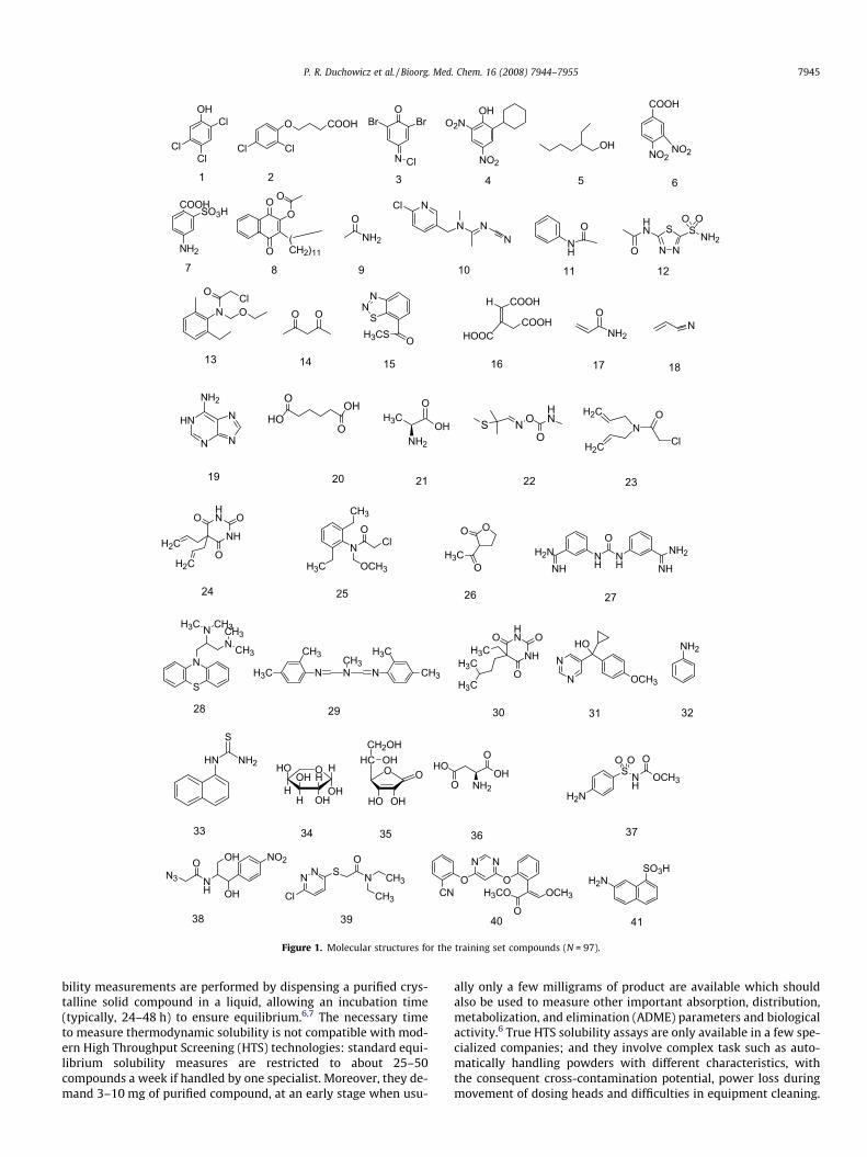
Figure 1. Molecular structures for the training set compounds (N = 97).

P. R. Duchowicz et al. / Bioorg. Med. Chem. 16 (2008) 7944–7955 7945

bility measurements are performed by dispensing a purified crys-talline solid compound in a liquid, allowing an incubation time(typically, 24–48 h) to ensure equilibrium.6,7 The necessary timeto measure thermodynamic solubility is not compatible with mod-ern High Throughput Screening (HTS) technologies: standard equi-librium solubility measures are restricted to about 25–50compounds a week if handled by one specialist. Moreover, they de-mand 3–10 mg of purified compound, at an early stage when usu-

ally only a few milligrams of product are available which shouldalso be used to measure other important absorption, distribution,metabolization, and elimination (ADME) parameters and biologicalactivity.6 True HTS solubility assays are only available in a few spe-cialized companies; and they involve complex task such as auto-matically handling powders with different characteristics, withthe consequent cross-contamination potential, power loss duringmovement of dosing heads and difficulties in equipment cleaning.

NH

HN

S O

H

HHHOOC

H3CH3C

NH

HNO O

O

HN O

Cl

O

Cl

O

OON

H

OH3C

CH3CH3

H2N HN 2

OCH3

ClO

Cl NO2

O

O

OF3C

ClH3C CH3

CH3

O

HO

O

HO O CH3

CH3

ONH

OH3C

OH3C

H3C

O N SO

CH3N CH3

CH3

S

O CH3

O

HN N

NN

Cl

O

O

CH3

F

H3C

O

FF

Cl

N

HN COOH

HN

O

NH2Cl

N NH

Cl

N

O

O

N

HN

HN NH2

COOHONH2

SO

O

OH

H COOH

HH3C HOOC

CH3

CH3

N N

N

Cl

HN

HNH3C

CN

CH3CH3

N N

N

OH

OHHO

NN CH3NH

HNO O

O

H3C H2N COOHH3C N

HNH

CNO O

NOCH3

N

NNCl

HOH3C

HN

N

N

CH3

OH

O

SNH2

HO

O

NH2S

OH3C

O

O

CH3

OO

CH3

CH3OH

OF

HO OHCH3H

H

42 43 44 45

46 47 48

49 50 51 52

53 54 55 56

57 58 59 60 61

62 63 64 65 66

67 68 69 70 71

Figure 1. (continued)

7946 P. R. Duchowicz et al. / Bioorg. Med. Chem. 16 (2008) 7944–7955

Kinetic solubility measurement starts from a pre-dissolvedsample of the compound, usually in dimethyl-sulfoxide (DMSO).Small volumes of the stock solution are added incrementally tothe aqueous solution of interest until the solubility limit is reached,the resulting precipitation being detected optically. Although fas-ter than thermodynamic solubility measurement, the DMSO mightwell operate as a co-solvent, dramatically enhancing the solubilityof lipophilic compounds.6 Because of these reasons and also be-cause the sample is in amorphous state, kinetic solubility tendsto overestimate thermodynamic solubility.

With this background, the use of QSPR methodologies to pre-dict aqueous solubility appears as an interesting, increasinglypopular alternative to solubility measurement: they are compa-tible with both HTS technologies and limited compound avail-ability typical of early stages of development, since none ofthe samples of compound is needed for the estimation of solu-bility and relatively few computational time is needed for thepredictions. Balakin et al. have proposed the following classifi-cation of in silico approaches for the assessment of aqueoussolubility3:

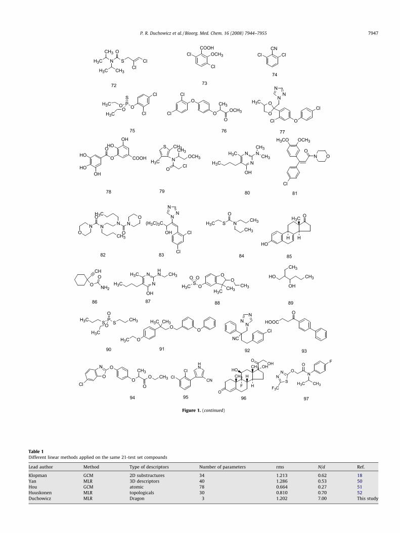
Table 1Different linear methods applied on the same 21-test set compounds

Lead author Method Type of descriptors Number of parameters rms N/d Ref.

Klopman GCM 2D substructures 34 1.213 0.62 18Yan MLR 3D descriptors 40 1.286 0.53 50Hou GCM atomic 78 0.664 0.27 51Huuskonen MLR topologicals 30 0.810 0.70 52Duchowicz MLR Dragon 3 1.202 7.00 This study

N S Cl

O

ClH3C CH3

H3C

CH3COOH

Cl OCH3

Cl

CNCl Cl

O

OOCH3

CH3

O

Cl

ClO

PS

OO

H3C

H3C

Cl

Cl

N

NN

O

Cl

Cl

O

O

H3C

HO

HOOH

O

OHO

OH

COOH

S

N

OCl

CH3OCH3

H3C

CH3

N

NH3C

H3C

OH

N CH3

CH3 ON O

Cl

OCH3H3CO

NO

N

ON N

O

O

CH3

H3CN

NN

(H3C)3C

OH

Cl

Cl

H3C S NCH3

O

CH3

O

HOH H

H3C

CH

O NH2

ON

N

H3C

HN CH3H3C

OH

HO CH3

CH3

OHH3CS

O

O O OO

CH3H3CCH3

OP SSO

CH3H3C

H3C OO

OH3C

H3C CH3 NN

N

ClNC

HOOC

O

O

OO CH3

CH3

O

O

N

Cl

HN

ClCl

CN

O

CH3

CH3OH

HO

O

OH

H

F H

F

N

OON

NS H3C CH3

F3C

72 73

74

75 76 77

78 79 80 81

82 83 84 85

86 87 88 89

90 91 92 93

94 95 96 97

Figure 1. (continued)

P. R. Duchowicz et al. / Bioorg. Med. Chem. 16 (2008) 7944–7955 7947

Table 2Experimental and predicted values for log10Sol (mg ml�1)

No. Chemical name Exp. Pred. Eq. (3)

Training set1 2,4,5-Trichlorophenol 0.079 �0.9432 2,4-DB �1.337 �1.293 2,6-Dibromoquinone-4-chlorimide �1.230 �1.1944 2-Cyclohexyl-4,6-dinitrophenol �1.823 �1.2755 2-Ethyl-1-hexanol �0.056 0.3216 3,4-Dinitrobenzoic acid 0.826 -0.5037 4-Amino-2-sulfobenzoic acid 0.477 0.1348 Acequinocyl �4.173 �4.5069 Acetamide 3.352 2.929

10 Acetamiprid 0.623 �0.611 Acetanilide 0.806 0.36312 Acetazolamide �0.009 1.76513 Acetochlor �0.652 �0.81214 Acetylacetone 2.221 1.97815 Acibenzolar-S-methyl �2.113 �0.21216 Aconitic acid 2.698 1.02117 Acrylamide 2.806 2.4618 Acrylonitrile 1.872 2.39619 Adenine 0.013 1.70620 Adipic acid 1.414 0.95121 Alanine 2.214 2.44122 Aldicarb 0.780 �0.11523 Allidochlor 1.294 �0.02224 Allobarbital 0.258 0.46825 Alochlor �0.620 �0.20826 Alpha-acetylbutyrolactone 2.301 1.45827 Amicarbalide 0.700 �0.28228 Aminopromazine �3.239 �1.93329 Amitraz �3.000 �2.53430 Amobarbital �0.220 0.49731 Ancymidol �0.187 �0.71932 Aniline 1.556 0.97933 ANTU �0.222 �0.66334 Arabinose 2.698 2.16835 Ascorbic acid 2.522 2.00536 Aspartic acid 0.912 2.09537 Asulam 0.699 �0.10638 Azidamfenicol 1.301 0.25839 Azintamide 0.699 �0.76240 Azoxystrobin �2.000 �3.39341 Badische acid �0.225 �0.81742 Barban �1.958 �2.24843 Barbital 0.873 0.85744 Bendiocarb �0.585 �0.59645 Benzidine �0.495 �1.02646 Bifenox �3.397 �3.20747 Bifentrhin �4.000 �3.548 Biotin �0.658 �0.21749 Capric acid �1.209 �0.51150 Caproic acid 1.012 1.12851 Carbofuran �0.495 �0.83652 Carbosulfan �3.522 �2.29653 Carboxin �0.701 �0.27454 Carfentrazone-ethyl �1.657 �2.22655 Carisoprodol �0.523 1.08856 Carmustine 0.602 0.59757 Carnosine 1.914 0.79158 1,6-Cleve’s acid 0.000 �0.57759 Crotonic Acid 1.934 1.78860 Cumic Acid �0.821 �0.40461 Cyanazine �0.767 �0.41762 Cyanuric Acid 0.301 1.61463 Cyclizine 0.000 �1.52564 Cyclobarbital 0.204 0.24165 Cycloleucine 1.698 1.18366 Cymoxanil �0.051 1.39167 Cyproconazole �0.854 �1.39968 Cyprodinil �1.886 �1.5869 Cystine �0.951 0.78170 Dehydroacetic Acid �0.161 0.99771 Dexamethasone �1.051 �0.78572 Diallate �1.853 �1.15473 Dicamba �0.080 �1.00374 Dichlobenil �1.673 �0.70575 Dichlofenthion �3.610 �2.456

Table 2 (continued)

No. Chemical name Exp. Pred. Eq. (3)

76 Diclofop-methyl �3.096 �3.0877 Difenoconazole �1.823 �3.46978 Digallic Acid �0.301 �0.8779 Dimethenamid 0.079 �0.95180 Dimethirimol 0.079 0.01981 Dimethomorph �1.728 �1.96682 Dimorpholamine 2.698 1.11883 Diniconazole �2.397 �1.72584 EPTC �0.426 �0.06585 Equilin �2.850 �2.38586 Ethinamate 0.398 �0.06487 Ethirimol �0.699 �0.2688 Ethofumesate �1.301 �1.04489 Ethohexadiol 1.623 0.77290 Ethoprop �0.125 �0.37791 Etofenprox �6.000 �3.45692 Fenbuconazole �3.699 �2.24893 Fenbufen �2.656 �2.07294 Fenoxaprop-ethyl �3.046 �3.22895 Fenpiclonil �2.318 �1.3596 Fludrocortisone �0.854 �1.20497 Flufenacet �1.252 �1.213

Test set val98 Flufenamic acid �2.041 �1.58599 Flumioxazin �2.747 �2.17

100 Fluspirilene �2.000 �4.587101 Fluthiacet-methyl �3.070 �2.002102 Folic acid �2.795 �2.532103 Fumaric acid 0.845 2.145104 Furametpyr �0.648 �0.611105 Furazolidone �1.397 0.07106 Ganciclovir 0.633 0.997107 Gluconolactone 2.770 1.776108 Glutamic acid 0.933 1.717109 Glycine 2.396 2.883110 Glyphosate 1.079 1.729111 Guaifenesin 1.698 0.936112 Haloperidol �1.853 �2.916113 Heptabarbital �0.602 �0.651114 Hexazinone 1.519 �0.268115 Histidine 1.658 1.705116 Hydrocortisone �0.495 �1.325117 Hydroflumethiazide �0.523 �0.956118 Hydroquinone 1.857 1.128119 Hydroxyphenamate 1.397 0.05120 Hydroxyproline 2.557 1.917121 Hymexazol 1.929 2.116122 Idoxuridine 0.301 0.688123 Imazapyr 1.053 �0.193124 Imazaquin �1.045 �1.316125 Imazethapyr 0.146 �0.625126 Iridomyrmecin 0.301 �0.272127 Isoflurophate 1.187 0.614128 Isoleucine 1.536 1.384129 Isoniazid 2.146 1.64130 Isophorone 1.079 0.542131 Ketanserin �2.000 �2.602132 Khellin 0.017 �0.417133 Lenacil �2.221 �0.913134 Linuron �1.124 �1.373135 Methomyl 1.763 0.648136 PABA 0.769 0.586137 p-Fluorobenzoic acid 0.079 0.349138 Phthalazine 1.698 0.776139 Phthalic Acid 0.846 0.228140 Phthalimide �0.444 0.303141 p-Hydroxybenzoic Acid 0.699 0.645142 Picloram �0.367 �0.035143 Picric Acid 1.103 �0.426144 Pirimicarb 0.431 �0.424145 Thionazin 0.057 0.222

Test set 21146 2,20 ,4,5,50-PCB �5.376 �3.932147 Benzocaine �0.102 0.104148 Theophylline 0.886 1.316

7948 P. R. Duchowicz et al. / Bioorg. Med. Chem. 16 (2008) 7944–7955

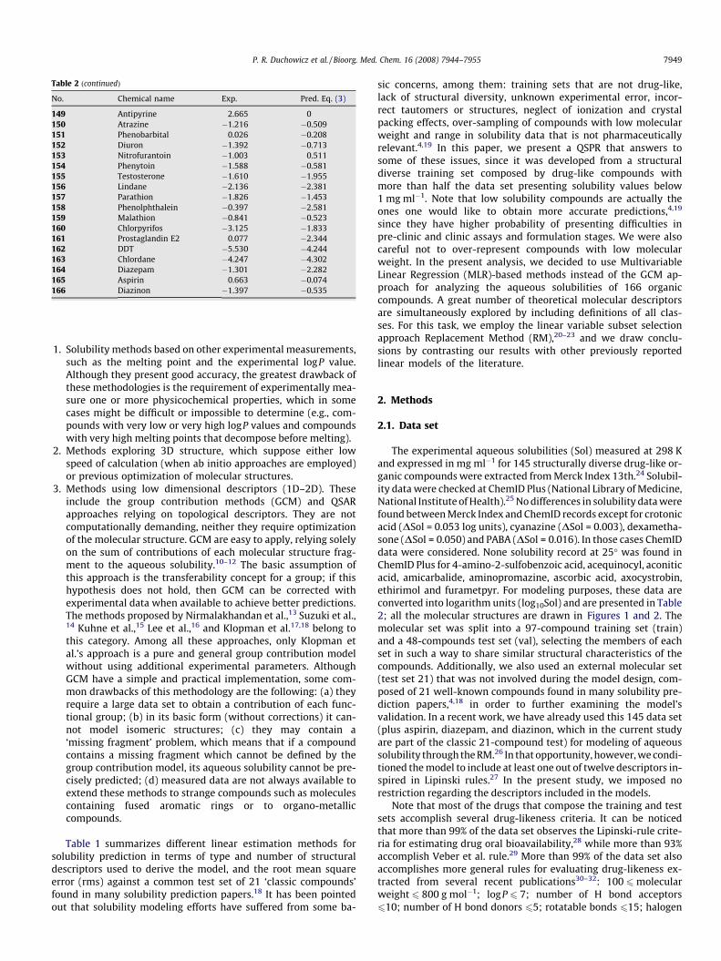
Table 2 (continued)

No. Chemical name Exp. Pred. Eq. (3)

149 Antipyrine 2.665 0150 Atrazine �1.216 �0.509151 Phenobarbital 0.026 �0.208152 Diuron �1.392 �0.713153 Nitrofurantoin �1.003 0.511154 Phenytoin �1.588 �0.581155 Testosterone �1.610 �1.955156 Lindane �2.136 �2.381157 Parathion �1.826 �1.453158 Phenolphthalein �0.397 �2.581159 Malathion �0.841 �0.523160 Chlorpyrifos �3.125 �1.833161 Prostaglandin E2 0.077 �2.344162 DDT �5.530 �4.244163 Chlordane �4.247 �4.302164 Diazepam �1.301 �2.282165 Aspirin 0.663 �0.074166 Diazinon �1.397 �0.535

P. R. Duchowicz et al. / Bioorg. Med. Chem. 16 (2008) 7944–7955 7949

1. Solubility methods based on other experimental measurements,such as the melting point and the experimental logP value.Although they present good accuracy, the greatest drawback ofthese methodologies is the requirement of experimentally mea-sure one or more physicochemical properties, which in somecases might be difficult or impossible to determine (e.g., com-pounds with very low or very high logP values and compoundswith very high melting points that decompose before melting).

2. Methods exploring 3D structure, which suppose either lowspeed of calculation (when ab initio approaches are employed)or previous optimization of molecular structures.

3. Methods using low dimensional descriptors (1D–2D). Theseinclude the group contribution methods (GCM) and QSARapproaches relying on topological descriptors. They are notcomputationally demanding, neither they require optimizationof the molecular structure. GCM are easy to apply, relying solelyon the sum of contributions of each molecular structure frag-ment to the aqueous solubility.10–12 The basic assumption ofthis approach is the transferability concept for a group; if thishypothesis does not hold, then GCM can be corrected withexperimental data when available to achieve better predictions.The methods proposed by Nirmalakhandan et al.,13 Suzuki et al.,14 Kuhne et al.,15 Lee et al.,16 and Klopman et al.17,18 belong tothis category. Among all these approaches, only Klopman etal.’s approach is a pure and general group contribution modelwithout using additional experimental parameters. AlthoughGCM have a simple and practical implementation, some com-mon drawbacks of this methodology are the following: (a) theyrequire a large data set to obtain a contribution of each func-tional group; (b) in its basic form (without corrections) it can-not model isomeric structures; (c) they may contain a‘missing fragment’ problem, which means that if a compoundcontains a missing fragment which cannot be defined by thegroup contribution model, its aqueous solubility cannot be pre-cisely predicted; (d) measured data are not always available toextend these methods to strange compounds such as moleculescontaining fused aromatic rings or to organo-metalliccompounds.

Table 1 summarizes different linear estimation methods forsolubility prediction in terms of type and number of structuraldescriptors used to derive the model, and the root mean squareerror (rms) against a common test set of 21 ‘classic compounds’found in many solubility prediction papers.18 It has been pointedout that solubility modeling efforts have suffered from some ba-

sic concerns, among them: training sets that are not drug-like,lack of structural diversity, unknown experimental error, incor-rect tautomers or structures, neglect of ionization and crystalpacking effects, over-sampling of compounds with low molecularweight and range in solubility data that is not pharmaceuticallyrelevant.4,19 In this paper, we present a QSPR that answers tosome of these issues, since it was developed from a structuraldiverse training set composed by drug-like compounds withmore than half the data set presenting solubility values below1 mg ml�1. Note that low solubility compounds are actually theones one would like to obtain more accurate predictions,4,19

since they have higher probability of presenting difficulties inpre-clinic and clinic assays and formulation stages. We were alsocareful not to over-represent compounds with low molecularweight. In the present analysis, we decided to use MultivariableLinear Regression (MLR)-based methods instead of the GCM ap-proach for analyzing the aqueous solubilities of 166 organiccompounds. A great number of theoretical molecular descriptorsare simultaneously explored by including definitions of all clas-ses. For this task, we employ the linear variable subset selectionapproach Replacement Method (RM),20–23 and we draw conclu-sions by contrasting our results with other previously reportedlinear models of the literature.

2. Methods

2.1. Data set

The experimental aqueous solubilities (Sol) measured at 298 Kand expressed in mg ml�1 for 145 structurally diverse drug-like or-ganic compounds were extracted from Merck Index 13th.24 Solubil-ity data were checked at ChemID Plus (National Library of Medicine,National Institute of Health).25 No differences in solubility data werefound between Merck Index and ChemID records except for crotonicacid (DSol = 0.053 log units), cyanazine (DSol = 0.003), dexametha-sone (DSol = 0.050) and PABA (DSol = 0.016). In those cases ChemIDdata were considered. None solubility record at 25� was found inChemID Plus for 4-amino-2-sulfobenzoic acid, acequinocyl, aconiticacid, amicarbalide, aminopromazine, ascorbic acid, axocystrobin,ethirimol and furametpyr. For modeling purposes, these data areconverted into logarithm units (log10Sol) and are presented in Table2; all the molecular structures are drawn in Figures 1 and 2. Themolecular set was split into a 97-compound training set (train)and a 48-compounds test set (val), selecting the members of eachset in such a way to share similar structural characteristics of thecompounds. Additionally, we also used an external molecular set(test set 21) that was not involved during the model design, com-posed of 21 well-known compounds found in many solubility pre-diction papers,4,18 in order to further examining the model’svalidation. In a recent work, we have already used this 145 data set(plus aspirin, diazepam, and diazinon, which in the current studyare part of the classic 21-compound test) for modeling of aqueoussolubility through the RM.26 In that opportunity, however, we condi-tioned the model to include at least one out of twelve descriptors in-spired in Lipinski rules.27 In the present study, we imposed norestriction regarding the descriptors included in the models.

Note that most of the drugs that compose the training and testsets accomplish several drug-likeness criteria. It can be noticedthat more than 99% of the data set observes the Lipinski-rule crite-ria for estimating drug oral bioavailability,28 while more than 93%accomplish Veber et al. rule.29 More than 99% of the data set alsoaccomplishes more general rules for evaluating drug-likeness ex-tracted from several recent publications30–32: 100 6molecularweight 6 800 g mol�1; logP 6 7; number of H bond acceptors610; number of H bond donors 65; rotatable bonds 615; halogen

NHN

N

O

COOH

CH3CH3

CH3

HN

COOHCF3

F O

N

O

O

N O

CH NH

NN

O

F

F

NN S

N

O

F

ClS

OCH3

O

N

HN

N

NH2N

O

HN

HN COOH

O COOH

O

HO

O

OH

NNCH3

Cl

H3C

HN

O

OH3C

CH3

CH3

OO2NN N

O

O HN

N N

NO

H2N

O

H OH

HOO

OH

OHHO

O

HO

OH

O

HO

O

NH2

H2NOH

O

PO

OHOH

HNHOOC

OCH3

OOH

OH N

OHO

FCl

NH

HNO O

OH3C

N N

NCH3

O

ONH3C

CH3

OH

O

HNN NH2

OO

O

HO

ON

CH3

CH3OH

H

H H

S NH

O O

NH

F3C

H2N SO O

OH

HO

O NH2

O

HO CH3OH

O

NHHO N

NHIO

OO

HO

OH

NO

OH

H3C

N

COOH

HN

N CH3

O

CH3

CH3N

COOH

HN

N CH3

O

CH3

CH3

H3C

O

H

H CH3

O

CH3

98 99 100 101

102 103 104

105 106 107 108 109

110 111 112 113

114 115 116 117

118 119 120 121 122

123 124 125 126

Figure 2. Molecular structures for the test set compounds (N = 48).

7950 P. R. Duchowicz et al. / Bioorg. Med. Chem. 16 (2008) 7944–7955

atoms 67; alkyl chains 6 (CH2)6CH3; no perfluorinated chains:CF2CF2CF3; no big size ring with more than seven members; nopresence of other atoms than C, O, N, S, P, F, Cl, Br, I, Na, K, Mg,Ca or Li and; presence of at least one N or O atom. Moreover, notethat low molecular weight compounds are not over-represented inthis molecular set. The structural diversity of the training set wasassessed through calculation of the average Tanimoto intermolec-ular distances (based on atom pairs) for all the possible pairs ofstructures that could be derived from the training set. For this pur-

pose, we used de PowerMV software provided by the NationalInstitute of Statistical Sciences.33 According to the results, the aver-age Tanimoto intermolecular distance for the training set is 0.781with a SD of 0.412, which confirms the high structural diversityof the training set. Figure 3 includes a histogram representingthe distribution of the 166 aqueous solubilities under study, whichsuggests that the experimental sample is normally distributed overmore than four logarithmic units and can thus be employed inregression analysis.

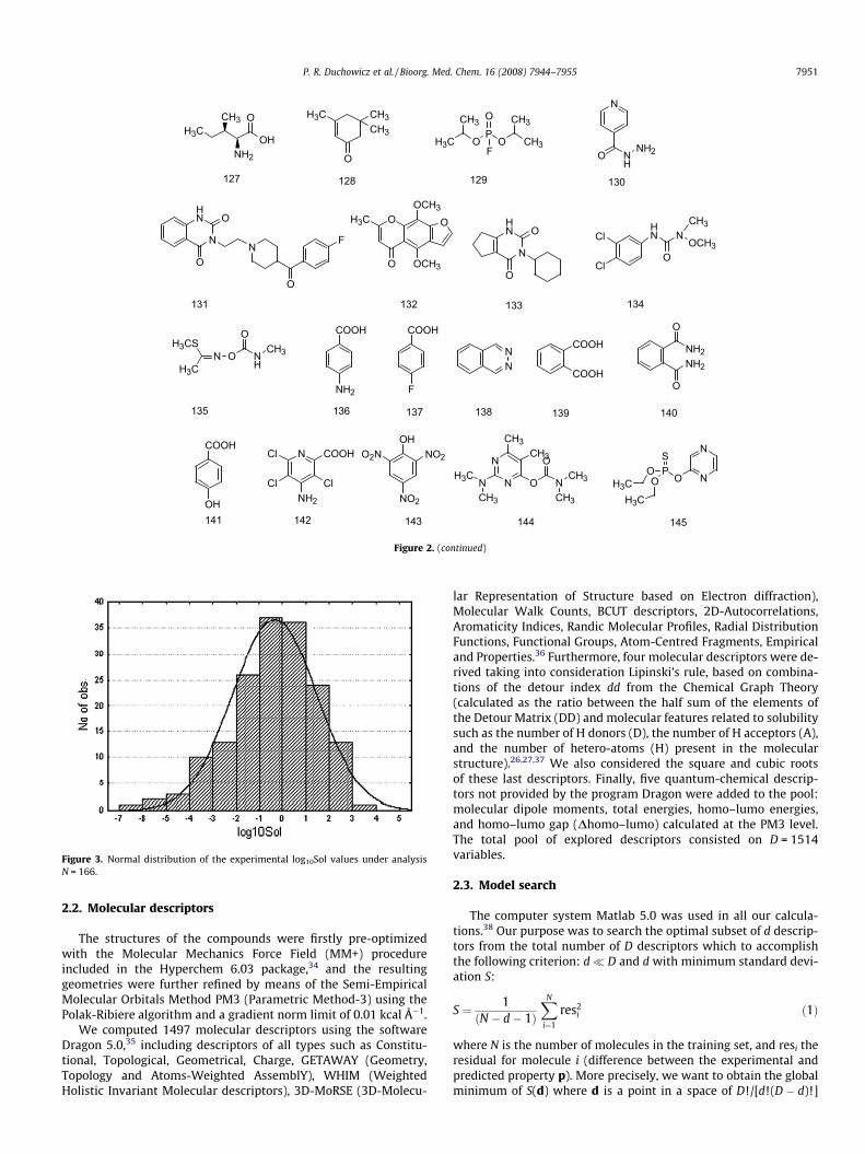
Figure 3. Normal distribution of the experimental log10Sol values under analysisN = 166.

N

O NH

NH2O

P

O

CH3

CH3

OF

H3C

CH3

O

N

O

FN

HN

O

O

O

H3COCH3

OCH3

O

N

HN O

OCl

HN N

OOCH3

CH3Cl

NH3CS

H3CO

O

NH

CH3

COOH

NH2 F

COOH

NN

COOH

COOH

COOH

OH

NCl

ClNH2

Cl

COOHOH

O2N NO2

NO2

N

N

NCH3

H3C

CH3CH3

O N

OCH3

CH3

SP

OOO

H3CH3C N

N

NH2

O

NH2

O

H3C CH3CH3

O

OH

OH3C

CH3

NH2

127 128 129 130

131 132 133 134

135 136 137 138 139 140

141 142 143 144 145

Figure 2. (continued)

P. R. Duchowicz et al. / Bioorg. Med. Chem. 16 (2008) 7944–7955 7951

2.2. Molecular descriptors

The structures of the compounds were firstly pre-optimizedwith the Molecular Mechanics Force Field (MM+) procedureincluded in the Hyperchem 6.03 package,34 and the resultinggeometries were further refined by means of the Semi-EmpiricalMolecular Orbitals Method PM3 (Parametric Method-3) using thePolak-Ribiere algorithm and a gradient norm limit of 0.01 kcal �1.

We computed 1497 molecular descriptors using the softwareDragon 5.0,35 including descriptors of all types such as Constitu-tional, Topological, Geometrical, Charge, GETAWAY (Geometry,Topology and Atoms-Weighted AssemblY), WHIM (WeightedHolistic Invariant Molecular descriptors), 3D-MoRSE (3D-Molecu-

lar Representation of Structure based on Electron diffraction),Molecular Walk Counts, BCUT descriptors, 2D-Autocorrelations,Aromaticity Indices, Randic Molecular Profiles, Radial DistributionFunctions, Functional Groups, Atom-Centred Fragments, Empiricaland Properties.36 Furthermore, four molecular descriptors were de-rived taking into consideration Lipinski’s rule, based on combina-tions of the detour index dd from the Chemical Graph Theory(calculated as the ratio between the half sum of the elements ofthe Detour Matrix (DD) and molecular features related to solubilitysuch as the number of H donors (D), the number of H acceptors (A),and the number of hetero-atoms (H) present in the molecularstructure).26,27,37 We also considered the square and cubic rootsof these last descriptors. Finally, five quantum-chemical descrip-tors not provided by the program Dragon were added to the pool:molecular dipole moments, total energies, homo–lumo energies,and homo–lumo gap (Dhomo–lumo) calculated at the PM3 level.The total pool of explored descriptors consisted on D = 1514variables.

2.3. Model search

The computer system Matlab 5.0 was used in all our calcula-tions.38 Our purpose was to search the optimal subset of d descrip-tors from the total number of D descriptors which to accomplishthe following criterion: d� D and d with minimum standard devi-ation S:

S ¼ 1ðN � d� 1Þ

XN

i¼1

res2i ð1Þ

where N is the number of molecules in the training set, and resi theresidual for molecule i (difference between the experimental andpredicted property p). More precisely, we want to obtain the globalminimum of S(d) where d is a point in a space of D!/[d!(D � d)!]

Table 3Linear QSPR models established for the training set of aqueous solubilities (N = 97)

da Descriptors involved Rb Sc FITd Rlooe Sloo

f Rvalg Sval

h

1 DP03 0.722 1.257 1.053 0.708 1.283 0.794 1.0472 DP03, MLOGP 0.831 1.016 2.071 0.817 1.054 0.798 0.9833 X1sol, RDF060u, MLOGP 0.871 0.903 2.747 0.849 0.971 0.848 0.8994 X1sol, RDF060u, RDF020e, MLOGP 0.889 0.844 3.078 0.870 0.911 0.838 0.9865 Sp, nR09, H3D, Mor04u, MLOGP 0.895 0.829 2.991 0.878 0.890 0.891 0.758

The best relationship found appears in bold.a d: number of descriptors in the linear regression.b R: correlation coefficient of the model.c S: standard deviation of the model.d FIT: Kubinyi function.e Rloo: R of Leave-One-Out.f Sloo: S of Leave-One-Out.g Rval: R of validation test set.h Sval: S of validation test set.

Table 4Symbols for molecular descriptors involved in different models

Molecular descriptor Dima Type Description

DP03 3D Randic molecular profiles Molecular profile No. 3MLOGP 1D Properties Moriguchi octanol–water partition coefficientX1sol 2D Topological Solvation connectivity index chi-1RDF060u 3D Radial Distribution Function Radial distribution function – 6.0/unweightedRDF020e 3D Radial Distribution Function Radial distribution function – 2.0/weighted by atomic Sanderson electronegativitiesSp 0D Constitutional Sum of atomic polarizabilities (scaled on carbon atom)nR09 0D Constitutional Number of nine-membered ringsH3D 3D Geometrical 3D-Harary indexMor04u 3D 3D-MoRSE 3D-MoRSE-signal 04/unweighted

a Dim, dimensionality of the descriptor.

7952 P. R. Duchowicz et al. / Bioorg. Med. Chem. 16 (2008) 7944–7955

ones. Usually, a full search (FS) of optimal variables is unfeasible be-cause it requires D!/[d!(D � d)!] linear regressions. Some time agowe proposed the Replacement Method (RM) that produces linearQSPR-QSAR models that are quite close the FS ones with much lesscomputational work.20–23 This technique approaches the minimumof S by judiciously taking into account the relative errors of the coef-ficients of the least-squares model given by a set of d descriptorsd = {X1,X2, . . . ,Xd}. The RM gives models with better statisticalparameters than the Forward Stepwise Regression procedure andsimilar ones to the more elaborated Genetic Algorithms.39,40

The Kubinyi function (FIT)41 is a statistical parameter that clo-sely relates to the Fisher ratio (F), but avoids the main disadvan-tage of the latter that is too sensitive to changes in small dvalues and poorly sensitive to changes in large d values. The FIT(d)criterion has a low sensitivity to changes in small d values and asubstantially increasing sensitivity for large d values. The greaterthe FIT value the better the linear equation. It is given by the fol-lowing equation, where R(d) is the correlation coefficient for amodel with d descriptors.

FIT ¼ R2ðN � d� 1ÞðN þ d2Þð1� R2Þ

ð2Þ

2.4. Model internal validation

The theoretical ‘internal validation’ practiced over each devel-oped linear model is based on the Leave-More-Out Cross-Valida-tion procedure (l-n%-o),42 with n% representing the percentage ofmolecules removed from the training set. The number of casesfor random data removal analyzed in every l-n%-o is of 5,000,000.The percentage n% depends simultaneously upon the number ofcompounds (N), as one cannot remove many molecules from thetraining set if a small sample is analyzed as the normality condi-

tion of the fitted data has to be obeyed, and upon their structuraldiversity, since if the molecules are structurally very different,more compounds would have to be removed from the set forchecking the predictive performance of the model. We choosethe value of n% = 10% (10 compounds) in Cross-Validation in orderto properly validate the QSAR equations.

In addition, we applied the y-randomization technique43 withthe purpose of demonstrating that the model established doesnot result from happenstance but involves a real structure–prop-erty relationship. This method consists on scrambling the experi-mental property of each compound in such a way that it doesnot correspond to the respective compound. After analyzing5,000,000 cases of y-randomization for each developed QSPR, thesmallest S value obtained using this procedure turned out to be apoorer value when compared to the one found when consideringthe true calibration.

2.5. Orthogonalization procedure

We employ the orthogonalization procedure introduced severalyears ago by Randic44,45 as a way of improving the statistical inter-pretation of the model built by interrelated indices. From our pointof view, the co-linearity of the molecular descriptors should be aslow as possible, because the interrelatedness among the differentdescriptors can lead to highly unstable regression coefficients,which makes it impossible to know the relative importance of anindex and underestimates the utility of the regression coefficientsof the model. The crucial step of the orthogonalization process isthe choice of an appropriate order of orthogonalization, which inpresent analysis is the order that maximizes the correlation be-tween each orthogonal descriptor and the observed aqueous solu-bilities. From now on, an orthogonalized descriptor will berepresented with notation X.

P. R. Duchowicz et al. / Bioorg. Med. Chem. 16 (2008) 7944–7955 7953

3. Results and discussion

The application of the RM method on the training set of 97 het-erogeneous drugs leads to the best 1–5 variables linear regressionmodels listed in Table 3, while the specific details for all the molec-ular descriptors reported in this article are provided in Table 4. Aclose inspection of Table 3 reveals that the best linear QSPR equa-tion found for modeling the aqueous solubility of the organic com-pounds includes the following satisfactory three moleculardescriptors relationship:

log10Sol ¼ � 0:435ð�0:03Þ �XðX1solÞ � 0:503ð�0:06Þ �XðMLOGPÞþ 0:0767ð�0:01Þ �XðRDF060uÞ þ 2:970ð�0:3Þ ð3Þ

Figure 4. (a) Predicted (Eq. 3) versus experimental log10Sol for the training and testsets. (b) Dispersion plot of the residuals for the training and test sets according toEq. 3.

Ntrain = 97, Ntrain/d = 32.333, R = 0.871, S = 0.903, FIT = 2.747Rloo = 0.849, Sloo = 0.971, Rl�10%�o = 0.809, Sl�10%�o = 1.090,p < 10�4

Nval = 48, Rval = 0.848, Sval = 0.899

Here, the absolute errors of the regression coefficients are pro-vided in parentheses, p is the significance of the model, and loosub-index stands for the Leave-One-Out Cross-Validation tech-nique.42 The QSPR derived does not incorporate redundant struc-tural information, as it involves orthogonal descriptors.Furthermore, by means of a proper standardization39 of suchorthogonal variables it is feasible to assign a greater importanceto those molecular descriptors that exhibit larger absolute stan-dardized coefficients (st.coeff.). The order of appearance of eachdescriptor within the QSPR of Eq. 3 corresponds to its order ofimportance in the established relationship, and each variable in-cludes the following standardized coefficients: X(X1sol): 0.71,X(MLOGP): 0.42, and X(RDF060u): 0.28.

Table 2 also includes the predicted residuals as obtained via Eq.(3) for the training and test sets, while the plot of predicted versusexperimental aqueous solubilities shown in Figure 4a suggests thatthe 97 training and 48 test set val compounds follow a straight line.The behavior of the plotted residuals in terms of the predictions inFigure 4b leads to a normal distribution. This figure includes twocalibration outliers with a residual exceeding the value2S = 1.806: compounds 15 (Acibenzolar-S-Methyl, 1.902) and91(Etofenprox, �2.545), while none of the training compounds ex-ceed the value 3S = 2.709; the presence of these outliers may beattributed exclusively to be a pure consequence of the limitednumber of structural descriptors participating in Eq. 3, since thismodel have a high ratio of number of observations to number ofparameters (N/d = 32.333). The predictive power of the linear mod-el is satisfactory as revealed by its stability upon the inclusion orexclusion of compounds, as measured by the loo parametersRloo = 0.849 and Sloo = 0.971, and by the more severe test ofhigher percentage of compounds exclusion Rl�10%�o = 0.809 andSl�10% �o = 1.090. These results are in the range of a validated mod-el: Rl�n%�o must be greater than the value of 0.50, according to thespecialized literature.46 Furthermore, the predictive capability ofthe so-established equation is demonstrated by its performancein the test set val, leading to Rval = 0.848 and Sval = 0.899. Finally,after analyzing 5,000,000 cases fory-randomization, the smallestS value obtained using this procedure was 1.650, a poorer valuewhen compared to the one found considering the true calibration(S 0.903). In this way, the robustness of the model could beassessed, showing that the calibration was not a fortuitous correla-tion and therefore results in a structure–activity relationship.

The three structural descriptors mentioned in Eq. 3 quantify dif-ferent aspects of the molecular geometry and can be classified asfollows: (i) a topological 2D-descriptor: X1sol, the solvation con-nectivity index chi-1, (ii) a Property 1D-descriptor: MLOGP, the

Moriguchi octanol–water partition coefficient; and (iii) a RadialDistribution Function 3D-descriptor: RDF060u, the radial distribu-tion function �6.0/unweighted. As can be appreciated, differentdefinitions of descriptors are needed to correctly represent thestructures for the drug-like heterogeneous compounds. Figure 5 in-cludes the histograms of the 166 organic compounds for each ofthe three descriptors appearing in the optimal QSPR equationfound.

The most important structural factor of the model, the bi-dimensional descriptor X1sol, was proposed by Zefirov and Palyu-lin47 in 1991 in order to treat the enthalpies of non-specific solva-tion. For instance, the solvation enthalpy of propane (CH3CH2CH3)and di-methyl-mercury (CH3HgCH3) differs enormously, but bothof these molecules are represented by the same hydrogen depletedgraph, and, hence, have the identical topological indices which donot take into account atom types. The solvation index was createdexactly to differentiate such cases, having the following generalformula when calculated for hydrogen- and fluorine-depletedmolecular graphs:

Xmsol ¼ ð1=2mþ1ÞX ZiZj . . . Zk

ðdidj . . . dkÞ1=2 ð4Þ

where m is the order of index; summation is over all sub-graphs oforder m; didj . . .dk are connectivities of vertexes of sub-graph; and

Figure 5. Histograms for the molecular descriptors appearing in the QSPR solubilitymodel (N = 166).

7954 P. R. Duchowicz et al. / Bioorg. Med. Chem. 16 (2008) 7944–7955

ZiZj . . .Zk are coefficients characterizing the atom size, which coin-cide to the number of the period in the Periodic Table. The term1/2m+1 just normalizes values of Xmsol to provide their coincidencewith the connectivity index Xm for the elements of the second row.The second important descriptor involved in Eq. 3 corresponds tothe Moriguchi octanol–water partition coefficient,48 revealing thata compound’s hydrofobicity plays a crucial role in explaining theaqueous solubility data. Finally, the contribution of a 3D-Radial Dis-tribution Function49 helps to improve the predictive power of theQSPR. Such a kind of molecular descriptor defined for an ensembleof atoms may be interpreted as the probability distribution of find-ing an atom in a spherical volume of certain radius, incorporating

different types of atomic properties in order to differentiate the nat-ure and contribution of atoms to the property being modeled. Forthe case of RDF060u, the sphere radius is of 6.0 Å and no atomicproperty is employed, thus characterizing the molecular size.

It is feasible to discuss the numerical effect of the optimal sub-set of structural descriptors selected in Eq. 3 on the aqueous solu-bility predictions. Since the orthogonal descriptor X(X1sol) isnumerically positive for all the structures under study, its contri-bution to log10Sol results in a negative quantity, according to theregression coefficient (�0.435). This causes that chemical com-pounds displaying greater values of X(X1sol) would tend to exhibitlower predicted values of aqueous solubilities. For the case of theorthogonal variable X(MLOGP), drugs manifesting higher positivevalues of this descriptor would tend to manifest their preferenceto the octanol lipophilic phase rather than to the water phase,and according to the sign of the regression coefficient in Eq. 3(�0.503) would lead to a lower prediction of the aqueous solubil-ities. Finally, the tri-dimensional descriptor X(RDF060u) wouldtend to lead to higher predictions of log10Sol whenever it presentshigher numerical values.

Applying now the designed QSPR model of Eq. 3 to the classicaltest set 21, whose data are considered ‘unknown’ and that do notparticipate during the model development (as is the case of testset val), leads to a square root mean quadratic residual (rms) of1.202. The statistical quality achieved on this test set is comparableto that obtained by the previously reported models for aqueoussolubilities in Table 1, and the main advantage here is that onlythree molecular descriptors are employed to model the physicalproperty and thus leads to a favorable ratio N/d = 7. This equationresults in a superior predictive quality than that obtained by theGCM of Klopman (rms = 1.213) involving 34 parameters,18 and alsooutperforms the MLR of Yan (rms = 1.286) using 40 parameters.50

4. Conclusions

The chemical information encoded by three theoretical molecu-lar descriptors of the one-, two-, and three-types participating in alinear QSPR model enabled to explain the variation of the experi-mental aqueous solubilities in a satisfactory extent, and alloweda proper characterization of structurally heterogeneous drug-likeorganic compounds from both the training and test sets. The QSPRdesigned involved molecular descriptors that have a quite directinterpretation, and this relationship proved to have general appli-cability. The statistical parameters of the proposed model comparefairly well with others published previously based on Group Con-tribution methods. Furthermore, among the different linear regres-sion based-algorithms, the Replacement Method continuesdemonstrating to be an efficient technique for the search of a re-duced set of numerical variables from a huge number of them. Thishas application for the analysis of any physicochemical, biological,or pharmacological property of interest.

Acknowledgments

P.R.D. and A.T. thank to the National Council of Scientific andTechnological Research (CONICET) for supporting this work. L.B.B.thanks ANPCyT and Universidad Nacional de La Plata for support-ing this work.

References and notes

1. Schuster, D.; Laggner, C.; Langer, T. Curr. Pharm. Des. 2005, 11, 3545.2. Stegemann, S.; Leveiller, F.; Franchi, D.; de Jong, H.; Lindén, H. Eur. J. Pharm. Sci.

2007, 31, 249.3. Balakin, K. V.; Savchuk, N. P.; Tetko, I. V. Curr. Med. Chem. 2006, 13, 226.4. Delaney, J. S. Drug Discov. Today 2005, 10, 289.5. Goodwin, J. J. Drug Discov. Today Technol. 2006, 3, 67.

P. R. Duchowicz et al. / Bioorg. Med. Chem. 16 (2008) 7944–7955 7955

6. Alsenz, J.; Kansy, M. Adv. Drug Deliv. Rev. 2007, 59, 546.7. Bhattachar, S. N.; Deschenes, L.; Wesley, J. A. Drug Discov. Today 2006, 11, 1012.8. Di, L.; Kerns, E. H. Drug Discov. Today 2006, 11, 446.9. Smith, C. J.; Hansch, C. Food Chem. Toxicol. 2000, 38, 637.

10. Artist, http://www.ddbst.de/new/Win_DDBSP/frame_Artist.htm.11. ChemEng Software Design, http://www.cesd.com/chempage.htm.12. Predict, http://www.mwsoftware.com/dragon/desc.html.13. Nirmalakhandan, N. N. P.; Speece, R. E. Environ. Sci. Technol. 1989, 23, 708.14. Suzuki, T. J. Comput.-Aided Mol. Des. 1991, 5, 149.15. Kuhne, R.; Ebert, R. U.; Kleint, F.; Schmidt, G.; Schuurmann, G. Chemosphere

1995, 30, 2061.16. Lee, Y.; Myrdal, P. B.; Yalkowsky, S. H. Chemosphere 1996, 33, 2129.17. Klopman, G.; Zhu, H. J. Chem. Inf. Model. 2001, 41, 439.18. Klopman, G.; Wang, S.; Balthasar, D. M. J. Chem. Inf. Model. 1992, 32, 474.19. Johnson, S. R.; Zheng, W. AAPS J. 2006, 8, E27.20. Duchowicz, P. R.; Castro, E. A.; Fernández, F. M.; González, M. P. Chem. Phys.

Lett. 2005, 412, 376.21. Duchowicz, P. R.; Castro, E. A.; Fernández, F. M. MATCH Commun. Math. Comput.

Chem. 2006, 55, 179.22. Duchowicz, P. R.; Fernández, M.; Caballero, J.; Castro, E. A.; Fernández, F. M.

Bioorg. Med. Chem. 2006, 14, 5876.23. Helguera, A. M.; Duchowicz, P. R.; Pérez, M. A. C.; Castro, E. A.; Cordeiro, M. N.

D. S.; González, M. P. Chemometr. Intell. Lab. 2006, 81, 180.24. The Merck Index An Encyclopedia of Chemicals, Drugs, and Biologicals; Merck

& Co.: NJ, 2001.25. Division of Specialized Information Services, National Institute of Health.

ChemID Plus. http://chem.sis.nlm.nih.gov/chemidplus/.26. Duchowicz, P. R.; Talevi, A.; Bellera, C.; Bruno-Blanch, L. E.; Castro, E. A. Bioorg.

Med. Chem. 2007, 15, 3711.27. Talevi, A.; Castro, E. A.; Bruno-Blanch, L. E. J. Arg. Chem. Soc. 2006, 44, 129.28. Lipinski, C. A.; Lombardo, F.; Dominy, D. W.; Feeney, P. J. Adv. Drug Deliver. Rev.

2001, 46, 3.

29. Veber, D. F.; Johnson, S. R.; Cheng, H.; Smith, B. R.; Ward, K. W.; Kopple, K. D. J.Med. Chem. 2002, 45, 2615.

30. Charifson, P. S.; Walters, W. P. J. Comput. Aided Mol. Des. 2002, 16, 311.31. Monge, A.; Arrault, A.; Marot, C.; Morin-Allory, L. Mol. Divers. 2006, 10,

339.32. Walters, W. P.; Murcko, M. A. Adv. Drug Deliv. Rev. 2002, 54, 255.33. Liu, K.; Feng, J.; Young, S. S. J. Chem. Inf. Model. 2005, 45, 515. PowerMV v.0.61.

http://www.niss.org/PowerMV.34. Hyperchem 6.03 (Hypercube) http://www.hyper.com.35. Dragon 5.0, Evaluation Version, http://www.disat.unimib.it/chm.36. Todeschini, R.; Consonni, V. Handbook of Molecular Descriptors; Wiley VCH:

Weinheim, Germany, 2000.37. Harary, F. Graph Theory; Addison-Wesley, 1969.38. Matlab 7.0, The MathWorks Inc.39. Draper, N. R.; Smith, H. Applied Regression Analysis; John Wiley& Sons: New

York, 1981.40. So, S. S.; Karplus, M. J. Med. Chem. 1996, 39, 1521.41. Kubinyi, H. Quant.-Struct.-Act. Relat. 1994, 13, 393.42. Hawkins, D. M.; Basak, S. C.; Mills, D. J. Chem. Inf. Model. 2003, 43, 579.43. Wold, S.; Eriksson, L. Chemometrics Methods in Molecular Design; VCH:

Weinheim, 1995.44. Randic, M. J. Chem. Inf. Model. 1991, 31, 311.45. Randic, M. New J. Chem. 1991, 15, 517.46. Golbraikh, A.; Tropsha, A. J. Mol. Graphics Model. 2002, 20, 269.47. Antipin, I. S.; Arslanov, N. A.; Palyulin, V. A.; Konovalov, A. I.; Zefirov, N. S. Dokl.

Akad. Nauk. SSSR 1991, 316, 925 (Chem. Abstr. 115, 91390).48. Moriguchi, I.; Hirono, S.; Liu, Q.; Nakagome, I.; Matsuchita, Y. Chem. Pharm. Bull.

1992, 40, 127.49. Consonni, V.; Todeschini, R.; Pavan, M. J. Chem. Inf. Model. 2002, 42, 693.50. Yan, A.; Gasteiger, J. J. Chem. Inf. Model. 2003, 43, 429.51. Hou, T. J.; Xia, K.; Zhang, W.; Xu, X. J. J. Chem. Inf. Model. 2004, 44, 266.52. Huuskonen, J. J. Chem. Inf. Model. 2000, 40, 773.