New Interval Methodologies forReliable Chemical Process Modeling

Chao-Yang Gau∗ and Mark A. Stadtherr†

Department of Chemical EngineeringUniversity of Notre Dame

182 Fitzpatrick HallNotre Dame, IN 46556 USA

March 2001(revised, December 2001)

Keywords: Modeling, Nonlinear Equations, Optimization, Numerical Methods, Interval Analysis

∗Current address: LINDO Systems, Inc., 1415 North Dayton Street, Chicago, IL 60622, USA†Author to whom all correspondence should be addressed. Fax: (219) 631-8366; E-mail: markst@nd.edu

Abstract

The use of interval methods, in particular interval-Newton/generalized-bisection techniques, provides an

approach that is mathematically and computationally guaranteed to reliably solve difficult nonlinear equa-

tion solving and global optimization problems, such as those that arise in chemical process modeling. The

most significant drawback of the currently used interval methods is the potentially high computational cost

that must be paid to obtain the mathematical and computational guarantees of certainty. New methodolo-

gies are described here for improving the efficiency of the interval approach. In particular, a new hybrid

preconditioning strategy, in which a simple pivoting preconditioner is used in combination with the standard

inverse-midpoint method, is presented, as is a new scheme for selection of the real point used in formulating

the interval-Newton equation. These techniques can be implemented with relatively little computational

overhead, and lead to a large reduction in the number of subintervals that must be tested during the interval-

Newton procedure. Tests on a variety of problems arising in chemical process modeling have shown that

the new methodologies lead to substantial reductions in computation time requirements, in many cases by

multiple orders of magnitude.

1 Introduction

The need to solve systems of nonlinear equations is of course an important issue in the field of scientific

and engineering computation. For example, in chemical process modeling there is a frequent need to deal

with nonlinear models of physical phenomena and of the manufacturing processes exploiting these phenom-

ena. Nonlinear equation solving problems may arise directly in solving such models, or indirectly in solving

optimization problems based on the models. Because of the nonlinearity of the systems to be solved, a num-

ber of reliability issues arise. For example, a system may have multiple solutions. In some cases, findingall

the solutions may be necessary; in other cases, there may be only one physically correct solution, and some

assurance is needed that that solution is not missed. It may also be that a system has no solution. In this

situation, it is useful to know with certainty that this is in fact the case, and that failure to find a solution is

not due to some numerical or software issue. Furthermore, even if there is only a single solution, it may be

difficult to find using standard Newton or quasi-Newton techniques, since the convergence behavior of these

methods can be highly initialization dependent.

A wide variety of techniques have been introduced to try to address such reliability issues. For example,

trust-region approaches such as the dogleg method (e.g. Powell, 1970; Chen and Stadtherr, 1981; Lucia

and Liu, 1998) can improve convergence behavior. Homotopy-continuation methods (e.g., Wayburn and

Seader, 1987; Kuno and Seader, 1988; Sun and Seider, 1995; Jalali-Farahani and Seader, 2000) often provide

much improved reliability and also the capability for locating multiple solutions. However, all of these

approaches are still initialization dependent, and, except in some special cases, can provide no guarantee

that all solutions of the nonlinear system will be found. One approach to providing such guarantees is to

reformulate the equation solving problem as an optimization problem (e.g. Maranas and Floudas, 1995;

Harding et al., 1997; Harding and Floudas, 2000) and then apply powerful deterministic global optimization

techniques such as alpha-BB (Adjiman et al., 1998a,b), which employs a branch-and-bound methodology

using convex underestimating functions. This provides a mathematical guarantee that all solutions will be

located. However, to use this approach it may be necessary to perform problem reformulations and develop

convex underestimators specific to each new application.

Another approach for reliable nonlinear equation solving is the use of interval methods, in particular,

interval-Newton/generalized-bisection (IN/GB) techniques. This approach is mathematicallyand compu-

tationally guaranteed to find (or, more precisely, to enclose within very narrow intervals) any and all so-

lutions to a system of nonlinear equations. The computational guarantee is possible because the interval

1

methodology deals automatically with rounding error issues, and is emphasized since a purely mathemati-

cal guarantee may be lost once the technique offering it is implemented in floating point arithmetic. Good

introductions to the use of interval methods have been provided by Neumaier (1990), Hansen (1992), and

Kearfott (1996). While the use of interval techniques for nonlinear equation solving in process modeling

problems was originally explored some time ago (Shacham and Kehat, 1973), it has been only in recent

years that the methodology has been more widely studied (e.g., Schnepper and Stadtherr, 1996; Balaji and

Seader, 1995). Among the problems to which it has been successfully applied are phase stability analysis

(e.g., Stadtherr et al., 1995; McKinnon et al., 1996; Hua et al., 1996, 1998; Xu et al., 2000; Tessier et al.,

2000), computation of azeotropes (Maier et al., 1998, 2000), and parameter estimation in vapor/liquid equi-

librium models (Gau and Stadtherr, 2000a). Using the interval approach, these problems can be solved with

complete certainty. The methodology is general purpose and can be applied to a wide variety of equation

solving and optimization problems in process modeling.

The most significant drawback of the currently used interval methods is the potentially high computa-

tional cost (CPU time) that must be paid to obtain the mathematical and computational guarantees of cer-

tainty. In general, this has limited the size of problems that can be addressed using this methodology, though

problems involving over one hundred variables have been successfully solved (Schnepper and Stadtherr,

1996). We describe here new methodologies for improving the efficiency of the interval-Newton approach.

The focus is on the formulation and solution of the interval-Newton equation, a linear interval equation

system whose solution is a key step in the IN/GB algorithm. In particular, we consider the preconditioning

strategy used when solving the interval-Newton equation, and the selection of the real point used in formu-

lating the interval-Newton equation. The new techniques are tested using a variety of problems, leading to

large reductions in computation time requirements, in some cases by factors of two orders of magnitude or

more.

2 Background

2.1 Interval-Newton Method

A real intervalX is defined as the set of real numbers lying between (and including) given upper and

lower bounds; that is,X = [X,X ] = {x ∈ < | X ≤ x ≤ X}. Here an underline is used to indicate

the lower bound of an interval and an overline is used to indicate the upper bound. A real interval vector

2

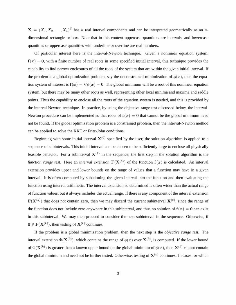
X = (X1,X2, . . . ,Xn)T hasn real interval components and can be interpreted geometrically as ann-

dimensional rectangle or box. Note that in this context uppercase quantities are intervals, and lowercase

quantities or uppercase quantities with underline or overline are real numbers.

Of particular interest here is the interval-Newton technique. Given a nonlinear equation system,

f(x) = 0, with a finite number of real roots in some specified initial interval, this technique provides the

capability to find narrow enclosures of all the roots of the system that are within the given initial interval. If

the problem is a global optimization problem, say the unconstrained minimization ofφ(x), then the equa-

tion system of interest isf(x) = ∇φ(x) = 0. The global minimum will be a root of this nonlinear equation

system, but there may be many other roots as well, representing other local minima and maxima and saddle

points. Thus the capability to enclose all the roots of the equation system is needed, and this is provided by

the interval-Newton technique. In practice, by using the objective range test discussed below, the interval-

Newton procedure can be implemented so that roots off(x) = 0 that cannot be the global minimum need

not be found. If the global optimization problem is a constrained problem, then the interval-Newton method

can be applied to solve the KKT or Fritz-John conditions.

Beginning with some initial intervalX(0) specified by the user, the solution algorithm is applied to a

sequence of subintervals. This initial interval can be chosen to be sufficiently large to enclose all physically

feasible behavior. For a subintervalX(k) in the sequence, the first step in the solution algorithm is the

function range test. Here aninterval extensionF(X(k)) of the functionf(x) is calculated. An interval

extension provides upper and lower bounds on the range of values that a function may have in a given

interval. It is often computed by substituting the given interval into the function and then evaluating the

function using interval arithmetic. The interval extension so determined is often wider than the actual range

of function values, but it always includes the actual range. If there is any component of the interval extension

F(X(k)) that does not contain zero, then we may discard the current subintervalX(k), since the range of

the function does not include zero anywhere in this subinterval, and thus no solution off(x) = 0 can exist

in this subinterval. We may then proceed to consider the next subinterval in the sequence. Otherwise, if

0 ∈ F(X(k)), then testing ofX(k) continues.

If the problem is a global minimization problem, then the next step is theobjective range test. The

interval extensionΦ(X(k)), which contains the range ofφ(x) overX(k), is computed. If the lower bound

of Φ(X(k)) is greater than a known upper bound on the global minimum ofφ(x), thenX(k) cannot contain

the global minimum and need not be further tested. Otherwise, testing ofX(k) continues. In cases for which

3

it is desired to find all the stationary points (or KKT points) rather than just the global minimum, then this

step can be turned off.

The next step is theinterval-Newton test. Here the linear interval equation system

F ′(X(k))(N(k) − x(k)) = −f(x(k)) (1)

is set up and solved for a new intervalN(k), whereF ′(X(k)) is an interval extension of the Jacobian of

f(x), andx(k) is a point in the interior ofX(k), usually taken to be the midpoint. It has been shown that any

root x∗ contained inX(k) is also contained in theimageN(k). This implies that if there is no intersection

betweenX(k) andN(k) then no root exists inX(k), and suggests the iteration schemeX(k+1) = X(k)∩N(k).

In addition to this iteration step, which can be used to tightly enclose a solution, it has been proven that if

N(k) is contained completely withinX(k), then there is auniqueroot contained in the current subinterval

X(k). Thus, after computation ofN(k) from Eq. (1), there are three possibilities: 1.X(k) ∩ N(k) = ∅,meaning there is no root in the current subintervalX(k) and it can be discarded; 2.N(k) ⊂ X(k), meaning

that there is a unique root in the current subintervalX(k); 3. Neither of the above. In the last case, if the

intersectionX(k)∩N(k) is sufficiently smaller thanX(k), one can proceed by reapplying the interval-Newton

test to the intersection. Otherwise, the intersection is bisected, and the resulting two subintervals added to

the sequence of subintervals to be tested. This approach is referred to as an interval-Newton/generalized-

bisection (IN/GB) method. At termination, meaning after all subintervals in the sequence (and thus the entire

initial search spaceX(0)) have been tested, the result is either enclosures for all the real roots off(x) = 0,

or the knowledge that no such roots exist. If desired, this technique can also be extended, as demonstrated,

for example, by Balaji and Seader (1995), to locate complex, not just real, zeros off(x). For additional

mathematical details, the monographs of Neumaier (1990), Hansen (1992), and Kearfott (1996) are very

useful.

When machine computations with interval arithmetic operations are done, the endpoints of an interval

are computed with a directed outward rounding. That is, the lower endpoint is rounded down to the next

machine-representable number and the upper endpoint is rounded up to the next machine-representable

number. In this way, through the use of interval, as opposed to floating point arithmetic, any potential

rounding error problems are eliminated. Overall, the IN/GB method described above provides a procedure

that is both mathematicallyandcomputationally guaranteed to find narrow enclosures of all solutions of the

nonlinear equation systemf(x) = 0, or to find the global minimum of the nonlinear functionφ(x). As a

framework for our implementation of the IN/GB method, we use appropriately modified routines from the

4

packages INTBIS (Kearfott et al., 1990) and INTLIB (Kearfott et al., 1994).

It should be emphasized that the enclosure, existence, and uniqueness properties discussed above, which

are the basis of the IN/GB method, can be derived without making any strong assumptions about the function

f(x) for which roots (zeros) are sought. The function must have afinite number of roots over the search

interval of interest; however, no special properties such as convexity or monotonicity are required, andf(x)

may have trancendental terms (e.g., Hua et al., 1998). It is assumed thatf(x) is continuous over each

interval being tested; however, it need not be continuously differentiable. Instead, as shown by Neumaier

(1990), f(x) need only be Lipschitz continuous over the interval of interest; thus, functions with slope

discontinuities can be handled. In order to apply the method, it must be possible to determine an interval

extension of the Jacobian matrix (or of the “Lipschitz matrix” iff(x) is not continuously differentiable).

In general, this requires having an analytic expression forf(x); thus, the interval approach is generally not

suitable if f(x) is some kind of “black box” function. One difficulty with the interval-Newton approach

is that if a solution occurs at a singular point (i.e., where the Jacobian off(x) is singular), then it is not

possible to obtain the result that identifies a unique solution. For such a case, the eventual result from the

IN/GB algorithm will be a very narrow interval for which all that can be concluded is that it may contain

one or more solutions. In other words, the algorithm will not miss the solution (so the guarantee to enclose

all solutions remains), but rather, will enclose it within a narrow interval which can then be examined using

an alternative methodology (e.g., Kearfott et al., 2000). This situation does not occur in any of the example

problems considered here.

For improving the efficiency of IN/GB methods, there are various approaches, including: 1. Methods

for dealing with the “dependency” issue in interval arithmetic, which may prevent the computation of inter-

val extensions that tightly bound the function range (e.g. Ratscheck and Rokne, 1984; Makino and Berz,

1999; Jansson, 2000); 2. Techniques that involve changes to the methodology at the level of the nonlinear

equation system (e.g., Alefeld et al., 1998; Granvilliers and Hains, 2000; van Hentenryck et al., 1997; Ratz,

1994; Herbort and Ratz, 1997; Yamamura et al., 1998; Yamamura and Nishizawa, 1999); 3. Methods that

seek to make improvements in solving the linear interval system defined by Eq. (1), the interval-Newton

equation (e.g., Kearfott, 1990; Hu, 1990; Kearfott et al., 1991; Gan et al., 1994; Hansen, 1997); or some

combination of the above (e.g., Madan, 1990; Dinkel et al., 1991; Kearfott, 1991; Kearfott, 1997). A com-

prehensive review or these and other techniques is beyond the scope of this paper. Our initial focus here

is on a methodology for solving the interval-Newton equation through the use of a hybrid preconditioning

5

technique. This combines a standard inverse-midpoint preconditioner with strategies developed from the

optimal preconditioning concepts of Kearfott and colleagues (Kearfott, 1990; Kearfott et al., 1991; Kearfott,

1996). Thus, we now provide some background on the solution of linear interval equation systems and on

these optimal preconditioning concepts.

2.2 Linear Interval Systems

Consider a linear interval equation systemAz = B, where the coefficient matrixA and the right-hand-

side vectorB are intervals. The solution setS of this linear interval system is generally defined to be the

set of all vectorsz that satisfy the real linear systemAz = b, whereA is any real matrix contained in

A andb is any real vector contained inB; that is,S = { z | Az = b, A ∈ A,b ∈ B}. However, as

discussed and illustrated by Hansen (1992) and Kearfott (1996), this set is in general not an interval, and

may have a very complex polygonal geometry. Thus to “solve” the linear system, one instead seeks an

interval (solution hull)Z containingS. Computing the exact solution hull (tightest interval containingS) is

NP-hard; however, it is generally relatively easy to obtain an intervalZ that contains, but may overestimate,

the exact solution hull. As discussed in detail by Kearfott (1996), the most common methods for doing this

are direct elimination methods (e.g., interval Gaussian elimination), interval Gauss-Seidel (e.g., Hansen and

Sengupta, 1981; Hansen and Greenburg, 1983), and the Krawczyk method (e.g., Krawczyk, 1969). For any

of these methods, the use of some preconditioning technique is necessary in practice to obtain reasonably

tight bounds on the solution set.

For the problem of interest, the interval-Newton equation, Eq. (1), the interval coefficient matrix is

A = F ′(X(k)), the interval extension of the Jacobian over the current subinterval, the interval right-hand

side is the degenerate (thin) intervalB whose components areBi = [−fi(x(k)),−fi(x(k))], and the solution

vector isN(k) − x(k). In the context of the interval-Newton method, the approach for solving the linear

system (i.e. bounding the solution set) that is most attractive (Kearfott, 1996) and widely used is interval

Gauss-Seidel, as described in more detail below.

2.3 Interval Gauss-Seidel

At the core of the interval-Newton method is the interval Gauss-Seidel procedure that is used to solve

Eq. (1) for the imageN(k). The interval-Newton equation is first preconditioned using a real matrixY (k).

6

The preconditioned linear interval equation system can then be expressed as

Y (k)F ′(X(k))(N(k) − x(k)) = −Y (k)f(x(k)) (2)

The preconditionerY (k) used here is commonly taken to be aninverse-midpoint preconditioner(Hansen,

1965; Hansen and Sengupta, 1981; Hansen and Greenburg, 1983), which may be either the inverse of the

real matrix formed from the midpoints of the elements of the interval JacobianF ′(X(k)), or the inverse of

the real matrix determined by evaluating the point Jacobianf ′(x) at the midpointx(k) of X(k).

Definingyi as the thei-th row of the preconditioning matrix, andAi as thei-th column of the interval

JacobianF ′(X(k)), then, beginning withX = X(k), the interval Gauss-Seidel scheme used in connection

with interval-Newton methods proceeds component by component according to

Ni = xi −yif(x) +

n∑j=1j 6=i

yiAj(Xj − xj)

yiAi(3)

= xi − Qi(yi)Di(yi)

,

whereyiAj indicates the inner product of the real row vectoryi and the interval column vectorAj, and

Qi(yi) andDi(yi) are, respectively the numerator and denominator in the final term in Eq. (3), expressed

as functions ofyi, and then

Xi ← Xi ∩Ni (4)

for i = 1, ..., n. Note that after componentNi of the image is calculated from Eq. (3) that the intersection

in Eq. (4) is immediately performed, and the updatedXi then used in the computation of subsequent

components of the image. This means that this procedure actually does not enclose the full solution set of

Eq. (1), but only the part of the solution set necessary for the interval-Newton iteration. Generally only one

pass is made through Eqs. (3–4) and so after all theXi have been updated the result isX = X(k+1), the

next interval-Newton iterate.

2.4 Preconditioners

The inverse-midpoint preconditioner is a good general-purpose preconditioner. However, as demon-

strated by Kearfott (1990), it is not always the most effective approach. Thus, it is possible to seek other

preconditioners that are optimal in some sense. The basic concepts in generating optimal preconditioners

7

for the interval Gauss-Seidel step were pioneered by Kearfott and colleagues (e.g., Kearfott, 1990; Kearfott

et al., 1991; Hu, 1990) and summarized in some detail by Kearfott (1996).

In these studies, a distinction is first made between contracting (C) and splitting (E) preconditioners. A

preconditioning rowyi is called a C-preconditioner if0 /∈ Di. In this case, since the denominator in Eq. (3)

does not contain zero, the resultingNi is a single connected interval. On the other hand, a preconditioning

row yi is called a E-preconditioner if0 ∈ Di, 0 6= Di and0 /∈ Qi. In this case, since the denominator in

Eq. (3) contains zero, an extended interval arithmetic (Kahan-Novoa-Ratz arithmetic) is needed to compute

Ni and the result is the union of two disconnected semi-infinite intervals [see Kearfott (1996) for details and

examples]. When used in the intersection step, Eq. (4), the resultingXi consists of two finite disconnected

intervals, and so an E-preconditioner can serve as a tessellation scheme in addition to the usual tessellation

done in the bisection step of the IN/GB algorithm.

For either C- or E-preconditioners, various optimality criteria can be defined, generally based on some

property ofNi. In the context of interval-Newton, the most useful are typically the width-optimal precon-

ditioner and the endpoint-optimal preconditioners. To determine a width-optimal preconditioner, elements

of yi are sought that minimize the width ofNi. To determine an endpoint-optimal preconditioner, elements

of yi are sought that either maximize the left endpoint (lower bound) or minimize the right endpoint (upper

bound) ofNi. Kearfott (1990) showed that, under some mild assumptions, these optimization problems

can be formulated and solved as linear programming (LP) problems. While the underlying optimization

problems haven degrees of freedom (then elements ofyi), the corresponding LP problems have at least

4n + 2 variables, as a number of auxiliary variables must be introduced in order to obtain the LP formu-

lation. Computational experience (Kearfott, 1990) has shown that, on some problems, the use of the LP

preconditioners can provide a significant reduction both in the number of subintervals that must be consid-

ered in the interval-Newton algorithm and in the overall CPU time required. However, in other problems,

the overhead required to implement the LP-based preconditioning scheme outweighed any reduction in the

number of subintervals tested, and overall CPU time actually increased. As one idea to make the optimal

preconditioners more practical, Kearfott (1990) suggested considering a sparse preconditioner, that is, one

in which only a small number of the elements ofyi are allowed to be nonzero. A special case of this, the

properties of which have been described by Kearfott et al. (1991), is the “pivoting” preconditioner, in which

there is only one nonzero element inyi. In the new hybrid preconditioning approach described below, the

concept of the pivoting preconditioner is adopted.

8

3 Hybrid Preconditioning Approach

We seek to develop an approach to preconditioning that results in a large reduction in the number of

subintervals that must be tested in the interval-Newton algorithm, but that also can be implemented with

little computational overhead, so that large savings in computation time can be realized. To do this we

adopt a hybrid approach in which a simple pivoting preconditioner is used in combination with the standard

inverse-midpoint scheme.

In a pivoting preconditioner, only one element of the preconditioning rowyi is nonzero, and it is assigned

a value of one. Thus, if elementj in yi is the “pivot element”, thenyij = 1 and all the other elements of

yi are zero. In applying such a preconditioning row in Eq. (3), the results forNi will obviously depend on

which elementj of yi is used as the pivot. This can be expressed as

(Ni)j = xi −(

Qi

Di

)j

, (5)

where

(Qi)j = fj(x) +n∑

k=1k 6=i

Ajk(Xk − xk) (6)

and

(Di)j = Aji (7)

Here and below, the notation( · )j is used to indicate a quantity that has been evaluated using elementj of

yi as the pivot in the pivoting preconditioner. Clearly, the results obtained for the image componentNi, and

thus the intersectionNi ∩ Xi, can be manipulated by choosing different elementsj to be the pivot. Thus,

some optimality criteria are needed to decide which elementj to choose.

In order to reduce the number of subintervals that must be tested during the interval-Newton algo-

rithm, an obvious goal is to reduce the number of bisections that occur. Bisections do not occur whenever

X(k) ∩N(k) = ∅, meaning there is no root in the current subintervalX(k) and it can be discarded, or when

N(k) ⊂ X(k), meaning that there is known to be a unique root in the current subintervalX(k), or if the

intersectionX(k) ∩N(k) is sufficiently smaller thanX(k), meaning that another interval-Newton test is tried

on X(k) ∩ N(k) rather than bisecting it. An optimality criterion that increases the likelihood of all these

possibilities is to seek to use a preconditioning rowyi that minimizes the width ofNi ∩Xi. This is treated

as two separate cases:

9

1. The rowyi is a “discarding-optimal” preconditioning row provided it results inNi ∩ Xi = ∅, indi-

cating thatNi ∩Xi has a minimum width of zero.

2. The rowyi is a “contraction-optimal” preconditioning row provided thatNi ∩ Xi is nonempty, and

that it minimizesw[Ni∩Xi], the width ofNi∩Xi. Note that this is somewhat different than the more

common width-optimal preconditioner that minimizes the width ofNi.

We will seek to find optimal pivoting preconditioners of these types. A pivoting preconditioner rowyi is

discarding-optimal if there is some pivot elementj in yi for which (Ni)j ∩Xi = ∅. A pivoting precondi-

tioner rowyi is contraction-optimal when the pivot elementj is the solution to the optimization problem

minj

w[(Ni)j ∩Xi]. If there exists a discarding-optimal rowyi, then there is no contraction-optimal row.

To look for a discarding-optimal pivoting preconditioner row, and, if none exists, to determine the

contraction-optimal pivoting preconditioner row, it is necessary to compute the endpoints of(Ni)j using

Eq. (5–7). Since these computations are done only for the purpose of selecting a preconditioning row, they

can be done cheaply using real (not interval) arithmetic. (Once the preconditioning row is chosen it must be

implemented in Eq. (3) using interval arithmetic.) Two cases must be considered, corresponding to the C-

and E-type preconditioners. If0 /∈ Aji, then we refer to elementj as a “C-pivot”; the right endpoint (upper

bound) of(Ni)j is then given by

R[(Ni)j ] = xi −min

{(Qi)jAji

,(Qi)jAji

,(Qi)jAji

,(Qi)jAji

}(8)

and the left endpoint (lower bound) by

L[(Ni)j ] = xi −max

{(Qi)jAji

,(Qi)jAji

,(Qi)jAji

,(Qi)jAji

}. (9)

If 0 ∈ Aji and 0 /∈ (Qi)j, then we refer to elementj as an “E-pivot”; for this case, Kahan-Novoa-

Ratz arithmetic is used, and(Ni)j = (Ni)−j ∪ (Ni)+j , the union of the semi-infinite intervals(Ni)−j =

[−∞, R[(Ni)−j ]] and(Ni)+j = [L[(Ni)+j ],∞], where for the case(Qi)j < 0, the finite bounds on(Ni)−jand(Ni)+j are given by

R[(Ni)−j ] = xi − (Qi)jAji

(10)

L[(Ni)+j ] = xi − (Qi)jAji

, (11)

and, for(Qi)j > 0, by

R[(Ni)−j ] = xi −(Qi)jAji

(12)

10

L[(Ni)+j ] = xi −(Qi)jAji

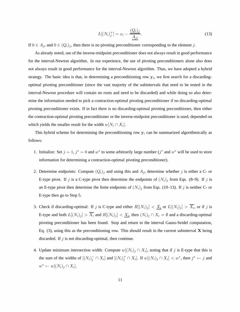
. (13)

If 0 ∈ Aji and0 ∈ (Qi)j , then there is no pivoting preconditioner corresponding to the elementj.

As already noted, use of the inverse-midpoint preconditioner does not always result in good performance

for the interval-Newton algorithm. In our experience, the use of pivoting preconditioners alone also does

not always result in good performance for the interval-Newton algorithm. Thus, we have adopted a hybrid

strategy. The basic idea is that, in determining a preconditioning rowyi, we first search for a discarding-

optimal pivoting preconditioner (since the vast majority of the subintervals that need to be tested in the

interval-Newton procedure will contain no roots and need to be discarded) and while doing so also deter-

mine the information needed to pick a contraction-optimal pivoting preconditioner if no discarding-optimal

pivoting preconditioner exists. If in fact there is no discarding-optimal pivoting preconditioner, then either

the contraction-optimal pivoting preconditioner or the inverse-midpoint preconditioner is used, depended on

which yields the smaller result for the widthw[Ni ∩Xi].

This hybrid scheme for determining the preconditioning rowyi can be summarized algorithmically as

follows:

1. Initialize: Setj = 1, j∗ = 0 andw∗ to some arbitrarily large number (j∗ andw∗ will be used to store

information for determining a contraction-optimal pivoting preconditioner).

2. Determine endpoints: Compute(Qi)j and using this andAji determine whetherj is either a C- or

E-type pivot. Ifj is a C-type pivot then determine the endpoints of(Ni)j from Eqs. (8–9). Ifj is

an E-type pivot then determine the finite endpoints of(Ni)j from Eqs. (10–13). Ifj is neither C- or

E-type then go to Step 5.

3. Check if discarding-optimal: Ifj is C-type and eitherR[(Ni)j] < Xi or L[(Ni)j ] > Xi, or if j is

E-type and bothL[(Ni)j ] > Xi andR[(Ni)j ] < Xi, then(Ni)j ∩Xi = ∅ and a discarding-optimal

pivoting preconditioner has been found. Stop and return to the interval Gauss-Seidel computation,

Eq. (3), using this as the preconditioning row. This should result in the current subintervalX being

discarded. Ifj is not discarding-optimal, then continue.

4. Update minimum intersection width: Computew[(Ni)j ∩ Xi], noting that ifj is E-type that this is

the sum of the widths of[(Ni)−j ∩Xi] and[(Ni)+j ∩Xi]. If w[(Ni)j ∩Xi] < w∗, thenj∗ ← j and

w∗ ← w[(Ni)j ∩Xi].

11

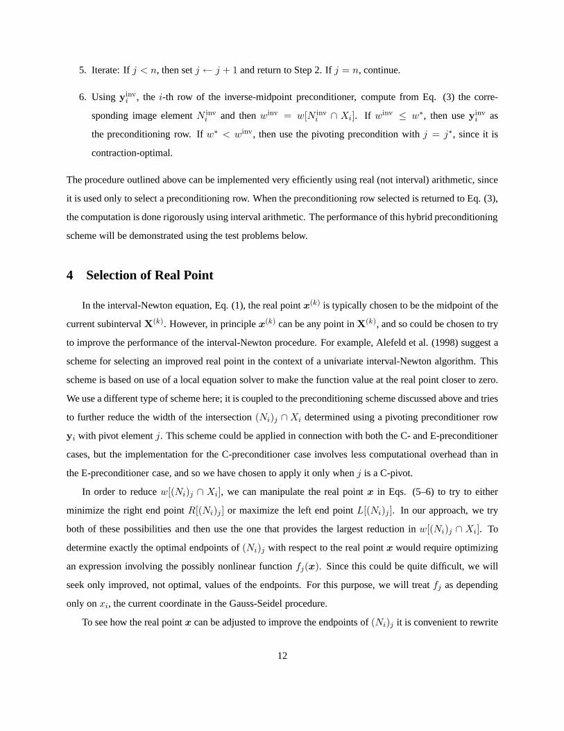
5. Iterate: Ifj < n, then setj ← j + 1 and return to Step 2. Ifj = n, continue.

6. Usingyinvi , the i-th row of the inverse-midpoint preconditioner, compute from Eq. (3) the corre-

sponding image elementN invi and thenwinv = w[N inv

i ∩ Xi]. If winv ≤ w∗, then useyinvi as

the preconditioning row. Ifw∗ < winv, then use the pivoting precondition withj = j∗, since it is

contraction-optimal.

The procedure outlined above can be implemented very efficiently using real (not interval) arithmetic, since

it is used only to select a preconditioning row. When the preconditioning row selected is returned to Eq. (3),

the computation is done rigorously using interval arithmetic. The performance of this hybrid preconditioning

scheme will be demonstrated using the test problems below.

4 Selection of Real Point

In the interval-Newton equation, Eq. (1), the real pointx(k) is typically chosen to be the midpoint of the

current subintervalX(k). However, in principlex(k) can be any point inX(k), and so could be chosen to try

to improve the performance of the interval-Newton procedure. For example, Alefeld et al. (1998) suggest a

scheme for selecting an improved real point in the context of a univariate interval-Newton algorithm. This

scheme is based on use of a local equation solver to make the function value at the real point closer to zero.

We use a different type of scheme here; it is coupled to the preconditioning scheme discussed above and tries

to further reduce the width of the intersection(Ni)j ∩Xi determined using a pivoting preconditioner row

yi with pivot elementj. This scheme could be applied in connection with both the C- and E-preconditioner

cases, but the implementation for the C-preconditioner case involves less computational overhead than in

the E-preconditioner case, and so we have chosen to apply it only whenj is a C-pivot.

In order to reducew[(Ni)j ∩ Xi], we can manipulate the real pointx in Eqs. (5–6) to try to either

minimize the right end pointR[(Ni)j ] or maximize the left end pointL[(Ni)j ]. In our approach, we try

both of these possibilities and then use the one that provides the largest reduction inw[(Ni)j ∩ Xi]. To

determine exactly the optimal endpoints of(Ni)j with respect to the real pointx would require optimizing

an expression involving the possibly nonlinear functionfj(x). Since this could be quite difficult, we will

seek only improved, not optimal, values of the endpoints. For this purpose, we will treatfj as depending

only onxi, the current coordinate in the Gauss-Seidel procedure.

To see how the real pointx can be adjusted to improve the endpoints of(Ni)j it is convenient to rewrite

12

Eq. (5–7) as

(Ni)j = xi − (Qi)jAji

= xi − fj(xi) + H

Aji(14)

whereH is the summation

H =n∑

k=1k 6=i

Ajk(Xk − xk). (15)

The non-current coordinatesxk, k 6= i, appear only in the termH/Aji. Thus to determine how to select

values of the non-current coordinates in the real point, we need only consider the effect of this last term on

the endpoints of(Ni)j . To try to best improve (increase)L[(Ni)j ], the values ofxk, k 6= i, that result in

the minimum upper bound forH should be sought ifAji > 0, and the values ofxk, k 6= i, that result in

the maximum lower bound forH should be sought ifAji < 0. Similarly, to try to best improve (decrease)

R[(Ni)j], the values ofxk, k 6= i, that result in the maximum lower bound forH should be sought if

Aji > 0, and the values ofxk, k 6= i, that result in the minimum upper bound forH should be sought if

Aji < 0.

Using Eq. (15), and remembering thatxk ∈ Xk, it can be determined that the values ofxk, k 6= i, that

minimizeH are given by

xk = x+k =

Xk if Ajk > 0

Xk if Ajk < 0Ajk(Xk)−Ajk(Xk)

Xk −Xkif 0 ∈ Ajk

(16)

and that the values ofxk, k 6= i, that maximizeH are given by

xk = x−k =

Xk if Ajk > 0

Xk if Ajk < 0Ajk(Xk)−Ajk(Xk)

Xk −Xkif 0 ∈ Ajk.

(17)

Thus, to try to increaseL[(Ni)j ], then, fork 6= i, choosexk = x+k if Aji > 0 andxk = x−

k if Aji < 0, and

to try to decreaseR[(Ni)j ], then, fork 6= i, choosexk = x−k if Aji > 0 andxk = x+

k if Aji < 0. Note that

these choices will not necessarily have the desired effect, since the dependence offj onxk, k 6= i, has been

neglected. Nevertheless, we have found this to be a useful scheme for many problems.

Selection of a value of the current coordinatexi to increaseL[(Ni)j ] or decreaseR[(Ni)j ] is less straight-

forward, since, depending on whether the choice is made based on thexi or thefj(xi)/Aji term in Eq. (14),

the choice will be different and contradictory. Looking just at thexi term,L[(Ni)j ] can be increased the

13

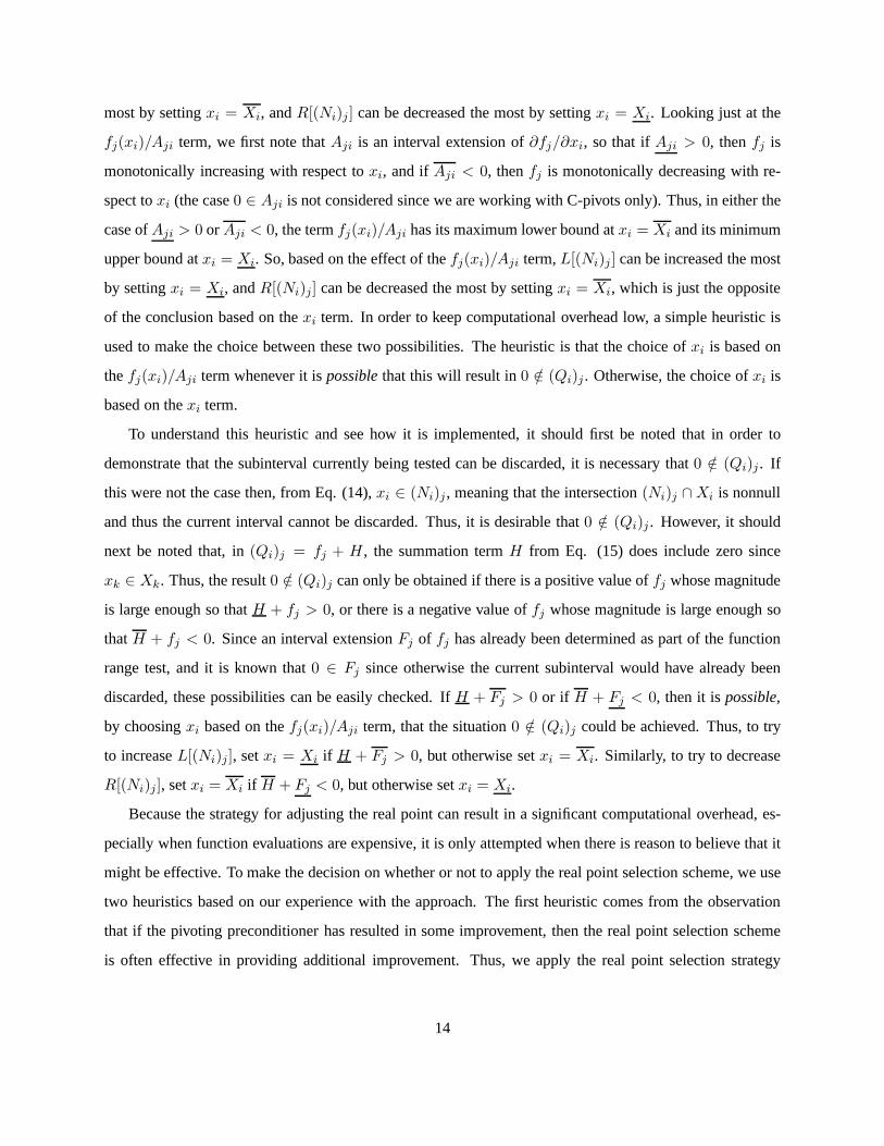
most by settingxi = Xi, andR[(Ni)j ] can be decreased the most by settingxi = Xi. Looking just at the

fj(xi)/Aji term, we first note thatAji is an interval extension of∂fj/∂xi, so that ifAji > 0, thenfj is

monotonically increasing with respect toxi, and if Aji < 0, thenfj is monotonically decreasing with re-

spect toxi (the case0 ∈ Aji is not considered since we are working with C-pivots only). Thus, in either the

case ofAji > 0 or Aji < 0, the termfj(xi)/Aji has its maximum lower bound atxi = Xi and its minimum

upper bound atxi = Xi. So, based on the effect of thefj(xi)/Aji term,L[(Ni)j ] can be increased the most

by settingxi = Xi, andR[(Ni)j] can be decreased the most by settingxi = Xi, which is just the opposite

of the conclusion based on thexi term. In order to keep computational overhead low, a simple heuristic is

used to make the choice between these two possibilities. The heuristic is that the choice ofxi is based on

thefj(xi)/Aji term whenever it ispossiblethat this will result in0 /∈ (Qi)j . Otherwise, the choice ofxi is

based on thexi term.

To understand this heuristic and see how it is implemented, it should first be noted that in order to

demonstrate that the subinterval currently being tested can be discarded, it is necessary that0 /∈ (Qi)j . If

this were not the case then, from Eq. (14),xi ∈ (Ni)j , meaning that the intersection(Ni)j ∩Xi is nonnull

and thus the current interval cannot be discarded. Thus, it is desirable that0 /∈ (Qi)j . However, it should

next be noted that, in(Qi)j = fj + H, the summation termH from Eq. (15) does include zero since

xk ∈ Xk. Thus, the result0 /∈ (Qi)j can only be obtained if there is a positive value offj whose magnitude

is large enough so thatH + fj > 0, or there is a negative value offj whose magnitude is large enough so

thatH + fj < 0. Since an interval extensionFj of fj has already been determined as part of the function

range test, and it is known that0 ∈ Fj since otherwise the current subinterval would have already been

discarded, these possibilities can be easily checked. IfH + Fj > 0 or if H + Fj < 0, then it ispossible,

by choosingxi based on thefj(xi)/Aji term, that the situation0 /∈ (Qi)j could be achieved. Thus, to try

to increaseL[(Ni)j ], setxi = Xi if H + Fj > 0, but otherwise setxi = Xi. Similarly, to try to decrease

R[(Ni)j], setxi = Xi if H + Fj < 0, but otherwise setxi = Xi.

Because the strategy for adjusting the real point can result in a significant computational overhead, es-

pecially when function evaluations are expensive, it is only attempted when there is reason to believe that it

might be effective. To make the decision on whether or not to apply the real point selection scheme, we use

two heuristics based on our experience with the approach. The first heuristic comes from the observation

that if the pivoting preconditioner has resulted in some improvement, then the real point selection scheme

is often effective in providing additional improvement. Thus, we apply the real point selection strategy

14

whenever, after Step 4 above,{w[Xi] − w[(Ni)j ∩ Xi]}/w[Xi] > ε1, whereε1 indicates some minimum

level of improvement. Currently we useε1 = 0, so if there is any improvement we proceed to apply the

real point selection scheme. The second heuristic is based on the observation that, even if(Ni)j ⊃ Xi,

some improvements may still be possible if the endpoints of(Ni)j are relatively close to the correspond-

ing endpoints ofXi. Thus, we also apply the real point selection scheme whenever, after Step 4 above,

{[Xi − (Ni)j ] + [(Ni)j − Xi]}/[Xi − Xi] = {w[(Ni)j ] − w[Xi]}/w[Xi] < ε2, where we currently use

ε2 = 0.1. This requires that both endpoints of(Ni)j be relatively close to the corresponding endpoints of

Xi. One might also use a heuristic requiring that only one endpoint of(Ni)j be close to the corresponding

endpoint ofXi, but this has not been tried. If neither of these two heuristic conditions is satisfied, then the

real point selection scheme is skipped for the current pivotj.

The scheme used to select a real pointx ∈ X is summarized algorithmically below. Note that this

procedure is coupled to the preconditioning scheme, and is implemented immediately after Step 4 in the

scheme outlined above.

4.1 Check for improved real point:

(a) (Check whether to skip) Setε1 andε2 (we useε1 = 0 andε2 = 0.1).

i. If 0 ∈ Aji, that is ifj is E-type, go to Step 5.

ii. If {w[Xi]− w[(Ni)j ∩Xi]}/w[Xi] > ε1, go to Step 4.1(b).

iii. If {w[(Ni)j ]− w[Xi]}/w[Xi] < ε2, then continue; otherwise, go to Step 5.

(b) (Check left endpoint) Computew[(Ni)j ∩Xi] using a trial real pointx, wherexk = x+, k 6= i,

if Aji > 0, or xk = x−, k 6= i, if Aji < 0, and usingxi = Xi if H + Fj > 0 or usingxi = Xi

otherwise. Ifw[(Ni)j ∩Xi] < w∗, thenx← x, j∗ ← j, andw∗ ← w[(Ni)j ∩Xi].

(c) (Check right endpoint) Computew[(Ni)j ∩Xi] using a trial real pointx, wherexk = x−, k 6= i,

if Aji > 0, or xk = x+, k 6= i, if Aji < 0, and usingxi = Xi if H + Fj < 0 or usingxi = Xi

otherwise. Ifw[(Ni)j ∩Xi] < w∗, thenx← x, j∗ ← j, andw∗ ← w[(Ni)j ∩Xi].

Note that if no change is made in the real pointx in either of Steps 4.1(b) or 4.1(c) above, thenx remains the

midpoint ofX. As in the case of the preconditioning scheme, the steps outlined above can be implemented

using real arithmetic. However, once the appropriate real point has been selected, the computation in Eq.

(3) must be done using interval arithmetic. Also note that, if a componentxk of the real point is selected to

be equal to an endpoint of the current subinterval, then before substitution into Eq. (3), a directed rounding

15

is done in order to ensure thatxk ∈ Xk. For example, if we setxk = Xk, thenxk is rounded up, and if we

setxk = Xk, thenxk is rounded down.

In the usual interval-Newton approach, ifNi ⊂ Xi for all componentsi in the Gauss-Seidel solution of

Eq. (1), then the conclusion is that there is a unique root in the current subintervalX. This same conclusion

is also valid when the preconditioning scheme described above is used, since this just means that a different

preconditioning matrix is used in solving for each different component in the Gauss-Seidel scheme. How-

ever, this conclusion is in general not valid when the real pointx is changed, as suggested above, with each

different component in the Gauss-Seidel procedure, since in this case a different formulation of the interval-

Newton equation is being used to compute each different componentNi of the image. Nevertheless, since

eachNi is computed from a valid form of the interval-Newton equation, it is still possible to conclude that if

there is a root whosei-th componentx∗i is in Xi thenx∗

i must be inNi, and thus the use of the intersection

Xi ∩ Ni to narrow or discard the current subinterval is still valid. If for some subinterval in which the

real point is changed, and the resultNi ⊂ Xi for all i is obtained, then to try to show that this subinterval

contains a unique root, we simply re-test this subinterval without use of the real point selection scheme

described here.

We now consider several example problems in which the performance of the interval-Newton method

with and without the new preconditioning and real point selection strategies is tested.

5 Numerical Experiments and Results

In this section, we present the results of numerical experiments done to test the effectiveness of the new

hybrid preconditioning strategy and real point selection scheme described above. The test problems include

a variety of global optimization and nonlinear equation solving problems arising in the context of process

systems engineering. For each case, all problem information, including detailed equation formulations,

equation parameters and other data, and the initial intervals used, are given in the references cited or in the

discussion below. All computations were performed on a Sun Ultra 2/1300 workstation.

5.1 Problem 1: Phase Stability Analysis

This problem involves the determination of phase stability from the UNIQUAC model of excess Gibbs

free energy (Tessier et al., 2000). The determination of phase stability is usually approached by using

tangent plane analysis, which states that a phase (or “feed”) at a specified temperatureT , pressureP , and

16

composition (mole fraction)z is not stable if the molar Gibbs energy vs. composition surfaceg(x) ever falls

below a plane tangent to the surface atz. That is, the feed is not stable if the tangent plane distance

D = g(x)− g0 −n∑

i=1

(∂g

∂xi

)0(xi − zi) (18)

is negative for any compositionx. Here the subscript zero indicates evaluation atx = z andn is the number

of components. To determine whetherD is ever negative, an optimization problem is solved in whichD is

minimized subject to1−∑ni=1 xi = 0. The stationary points in this optimization problem can be determined

by solving the nonlinear equation system

[(∂g

∂xi

)−

(∂g

∂xn

)]−

[(∂g

∂xi

)−

(∂g

∂xn

)]0

= 0, i = 1, . . . , n − 1 (19)

1−n∑

i=1

xi = 0. (20)

Thisn× n equation system is used here as an example problem to test the new interval methodologies. For

the case in whichg(x) is obtained using UNIQUAC, the details of the problem formulation are given by

Tessier et al. (2000), who solve the problem using an interval-Newton approach.

The specific problems considered are: 1. A four-component system of acetic acid, benzene, furfural

and cyclohexane 2. A five-component system containing the previous four components plus water. 3. A

six-component system of benzene, cyclohexane, 1,2-ethanediol, furfural, heptane, and water. The first two

problems were used by Tessier et al. (2000); the last is a new problem, with UNIQUAC parameters from

Sørensen and Arlt (1979–1987). For each system, the UNIQUAC model was used and and a number of dif-

ferent feed compositions were considered. For solving these problems we use the methodology described by

Tessier at al. (2000) for computing function extensions. This involves the use of monotonicity information

and the evaluation of functions in the constrained space for which the mole fractions sum to one. Because

this constrained-space extension requires that the components of the real point in the interval-Newton equa-

tions sum to one, we are unable to test the new real point selection scheme on this problem. Only the effect

of the new hybrid preconditioning strategy will be investigated. The initial intervals used in all cases is

xi ∈ [0, 1], i = 1, . . . , n.

All the problems considered were successfully solved, with the computational performance shown in

Tables 1–3. In these Tables, computational performance is indicated both by the number of subintervals that

needed to be considered in each case, as well as by the CPU time. Here “IMP” refers to the results for the

17

inverse-midpoint preconditioner, “HP” refers to the results for the new hybrid preconditioner, and “ImpFac”

refers to the improvement factor by which HP is better than IMP.

Looking first at the results for the four-component problem (Table 1), it is seen that the use of the

hybrid preconditioning scheme has resulted in an order of magnitude reduction in the number of subintervals

that needed to be considered in the interval-Newton algorithm. This is seen in the CPU time results as

well, though these improvement factors are not as large as in the number of subintervals, reflecting the

computational overhead required to implement the hybrid preconditioner. Based on an average over all the

tested feeds, the improvement factor due to use of the hybrid preconditioner is about 10.9 based on number

of subintervals and about 8.1 based on CPU time.

Not unexpectedly, improvement factors on the five- and six-component problems (Tables 2 and 3) are

even more pronounced, since there is increasingly more to gain on the larger problems. For the five-

component problem the average improvement factor is about 16.6 based on number of subintervals and

about 11.3 based on CPU time, while for the six-component problem the average improvement factors are

about 590 based on number of subintervals and about 425 based on CPU time. For the third feed considered

in the six-component problem, an improvement of three orders of magnitude was achieved in CPU time.

A problem that originally took over 40 hours to solve, could be solved in less than two-and-a-half minutes

when the new hybrid preconditioning strategy was used.

5.2 Problem 2: Mixture Critical Points

This problem involves the computation of mixture critical points from cubic equation-of-state models.

Stradi et al. (2001) have recently described how this can be accomplished reliably using an interval-Newton

methodology. In the problem formulation used by Stradi et al. (2001), the nonlinear equation system that

must be solved isC∑

j=1

Aij∆nj = 0, i = 1, . . . , C (21)

C∑i=1

C∑j=1

C∑k=1

Aijk∆ni∆nj∆nk = 0 (22)

1−C∑

i=1

∆(ni)2 = 0, (23)

whereAij andAijk represent the second and third order derivatives of the Helmholtz free energyA with

respect to composition, and are nonlinear functions of temperatureT and volumeV , both of which are

18

unknown. Also,C is the total number of components and the∆ni, i = 1, . . . , C, represent unknown

changes in the number of moles of theC components. This is a(C + 2)× (C + 2) equation system which

when solved forT , V , and∆ni, i = 1, . . . , C, yields the critical temperature and volume. For the cases

considered here,A(T, V ) is determined using the Peng-Robinson equation-of-state model. Details of the

problem formulation for this model, as well as model parameters and initial intervals used, are given by

Stradi (1999) and Stradi et al. (2001).

Three specific test problems are considered: 1. A three-component mixture of methane(1), carbon

dioxide(2), and hydrogen sulfide(3) with compositionx1 = 0.0700, x2 = 0.6160, andx3 = 0.3140; 2.

A four-component mixture of methane(1), ethane(2), propane(3), and nitrogen(4) with compositionx1 =

0.4345, x2 = 0.0835, x3 = 0.4330, andx4 = 0.0490; 3. A five-component mixture of methane(1),

ethane(2), propane(3),n-butane(4) and nitrogen(5) with compositionx1 = 0.9450, x2 = 0.0260, x3 =

0.0081, x4 = 0.0052, andx5 = 0.0160. For these problems, the effects of using both the new hybrid

preconditioning strategy and the new real point selection scheme are considered.

All the problems were successfully solved, with the computational performance shown in Table 4. Here

the notation is the same as above, but with the additional notation “HP/RP” to indicate use of both the hybrid

preconditioner and real point selection schemes. From these results, it can be seen first of all that use of

the real point selection scheme does have a beneficial effect, both on the number of subintervals and the

CPU time. The overall improvements, however, are much less dramatic than in the phase stability prob-

lem, and, also in contrast to the phase stability problem, the improvement factors decrease with increased

problem size. This behavior suggests that, for these problems, the dominant factor leading to computational

inefficiency is not in formulating or solving the interval-Newton equation, the factors addressed here, but

instead in obtaining reasonably tight bounds on the function and Jacobian element ranges when their interval

extensions are computed, a factor not addressed here. This overestimation in computing interval extensions

is due to the dependency problem, which may arise when a variable occurs more than once in a function

expression, and the interval extension is computed used interval arithmetic (the “natural” interval extension).

While a variable may take on any value within its interval, it must take on thesamevalue each time it occurs

in an expression. However, this type of dependency is not recognized when the natural interval extension

is computed. In effect, when the natural interval extension is used, the range computed for the function is

the range that would occur if each instance of a particular variable were allowed to take on a different value

in its interval range. The expressions for the functions and Jacobian elements for the critical point problem

19

are quite complicated, and grow increasingly so as the number of components increases, and so it is par-

ticularly difficult to get tight interval extensions using interval arithmetic. For the phase stability problem,

tighter interval extensions could be obtained by using the monotonicity and constrained-space extensions

described by Tessier et al. (2000). Similar techniques might be useful in improving the performance of the

interval-Newton algorithm on the mixture critical point problem.

5.3 Problem 3: Parameter Estimation in VLE Modeling

This is a problem that has also been used by Kim et al. (1990) and Esposito and Floudas (1998). It is a

parameter estimation problem using the error-in-variable (EIV) approach to estimate parameters in the van

Laar equation for activity coefficients used to model vapor-liquid equilibrium (VLE). These two parameters

are estimated from binary VLE data for the binary system of methanol and 1,2-dichloroethane. The ex-

perimental data consist of five experimental data points for four measured state variables, namely pressure,

temperature, liquid-phase mole fraction of methanol, and vapor-phase mole fraction of methanol. Complete

details of the problem are given by Gau and Stadtherr (2000b), who formulate it as an unconstrained global

optimization problem with 12 variables. A maximum-likelihood-based estimator is optimized by applying

the interval-Newton methodology to solve for the stationary points in the optimization problem. The ef-

fects of using both the new hybrid preconditioning strategy and the new real point selection scheme are

considered.

This global optimization problem was solved successfully, with computational performance results

shown in Table 5. When using the standard inverse-midpoint preconditioner, the program was still running

after two CPU days and was terminated at this point. However, when using the new hybrid preconditioner,

the problem was solved in only 1504.2 CPU seconds. When the real point selection scheme was also ap-

plied, the CPU time dropped to 807.9 CPU seconds. This is roughly half the CPU time required by Esposito

and Floudas (1998) to solve the problem on an HP 9000 C160 machine (which, based on the SPECfp95

benchmark, is a slightly faster machine than the Sun Ultra 2/1300 used here). Even if the problem had been

solved using the inverse-midpoint preconditioner after 2 CPU days, the improvement factor due to the use

of the new methodologies described here is over two orders of magnitude.

20

5.4 Problem 4: Parameter Estimation in Reactor Modeling

This is another problem from Kim et al. (1990) and Esposito and Floudas (1998). It is a parameter

estimation problem using the EIV approach to estimate kinetic parameters for an irreversible, first-order

reactionA → B, using data from an adiabatic CSTR. There are ten data points for five measured state

variables, namely the CSTR inlet and outlet temperatures, the outlet concentrations of A and B, and the inlet

concentration of A. Complete details of the problem are given by Gau and Stadtherr (2000b), who formulate

it as an unconstrained global optimization problem with 22 variables. Again a maximum-likelihood-based

estimator is optimized by using interval-Newton to determine the stationary points in the optimization prob-

lem, and the effects of using both the new hybrid preconditioning strategy and the new real point selection

scheme are considered.

This global optimization problem was successfully solved, with the results for computational perfor-

mance shown in Table 5. As in the previous problem, when the inverse-midpoint preconditioner alone was

used, the program was still executing after two CPU days and so was terminated without reaching a solu-

tion. However, when the hybrid preconditioning strategy was used the problem was solved in only 255.2

CPU seconds, and with the addition of the real point selection scheme, in only 28.8 CPU seconds. Relative

to the 2 CPU days spent without reaching a solution when the inverse midpoint preconditioner was used,

the improvement factor when using the new methodologies approaches four orders of magnitude. Again,

the solution time (28.8 CPU seconds) compares very favorably with that reported by Esposito and Floudas

(1998), who tried three different problem formulations, with a fastest solution time of 282.2 CPU seconds

on an HP 9000 C160, which, as noted above, is a slightly faster machine than the Sun Ultra 2/1300.

6 Concluding Remarks

We have described here new methodologies for improving the efficiency of the interval-Newton ap-

proach for the reliable solution of difficult global optimization and nonlinear equation solving problems. In

particular, we have presented a new hybrid preconditioning strategy, in which a simple pivoting precondi-

tioner is used in combination with the standard inverse-midpoint method, and a new scheme for selecting

the real point in formulating the interval-Newton equation. These techniques can be implemented with rel-

atively little computational overhead, and lead to a large reduction in the number of subintervals that must

be tested during the interval-Newton procedure. Tests on a variety of problems arising in chemical process

21

modeling have shown that the new methodologies lead to substantial reductions in CPU time requirements,

in many cases by multiple orders of magnitude. For each of the two parameter estimation examples, the

interval-Newton solution of the global optimization problem was essentially intractable using the standard

methodology; however, when the new strategies were applied, these problem could be solved easily.

The use of interval-Newton/generalized-bisection methods represents a powerful and general-purpose

approach to the solution of a number of difficult global optimization and nonlinear equation solving prob-

lems, such as arise in chemical process engineering. Continuing improvements in methodology, together

with advances in software (e.g., compilers that treat intervals as a standard data type) and hardware (e.g.,

faster processors and parallel computing) will make this an increasingly attractive problem solving tool.

Acknowledgments

This work has been supported in part by the donors of The Petroleum Research Fund, administered by

the ACS, under Grant 35979-AC9, by the National Science Foundation Grant EEC97-00537-CRCD, and by

the Environmental Protection Agency Grant R826-734-01-0.

22

References

Adjiman C. S., Dallwig, S., Floudas, C. A. & Neumaier, A. (1998a) A global optimization method, alpha

BB, for general twice-differentiable constrained NLPs – I. Theoretical advances.Comput. Chem.

Eng., 22, 1137.

Adjiman C. S., Androulakis, I. P. & Floudas, C. A. (1998b) A global optimization method, alpha BB,

for general twice-differentiable constrained NLPs – II. Implementation and computational results.

Comput. Chem. Eng., 22, 1159.

Alefeld, G. E., Potra, F. A., & Volker, W. (1998) Modifications of the interval-Newton-method with im-

proved asymptotic efficiency.BIT, 38, 619.

Balaji, G. V. & Seader, J. D. (1995) Application of interval-Newton method to chemical engineering prob-

lems.AIChE Symp. Ser., 91(304), 364.

Chen, H. S. & Stadtherr, M. A. (1981). A modification of Powell’s dogleg method for solving systems of

nonlinear equations.Comput. Chem. Eng., 5, 143.

Dinkel, J. J., Tretter, M., & Wong D. (1991). Some implementation issues associated with multidimen-

sional interval Newton methods.Computing, 47, 29.

Esposito, W. R. & Floudas, C. A. (1998). Global optimization in parameter estimation of nonlinear alge-

braic models via the error-in-variables approach.Ind. Eng. Chem. Res., 37, 1841.

Gau, C.-Y., Brennecke, J. F. & Stadtherr, M. A. (2000a) Reliable parameter estimation in VLE modeling.

Fluid Phase Equilib., 168, 1.

Gau, C.-Y. & Stadtherr, M. A. (2000b) Reliable nonlinear parameter estimation using interval analysis:

Error-in-variable approach.Comput. Chem. Eng., 24, 631.

Gan, Q., Yang, Q., & Hu, C. -Y. (1994) Parallel all-row preconditioned interval linear solver for nonlinear

equations on multiprocessors.Paral. Comput., 20, 1249.

Granvilliers, L. & Hains, G. (2000). A conservative scheme for parallel interval narrowing.Inform. Pro-

cess. Lett., 74, 141.

23

Hansen, E. (1965) Interval arithmetic in matrix computations, part I.J. SIAM Numer. Anal., 2, 308.

Hansen, E. R. (1992).Global Optimization Using Interval Analysis, Marcel Dekkar, New York, NY.

Hansen, E. R. (1997) Preconditioning linearized equations.Computing, 58, 187.

Hansen, E. R. & Greenberg, R. I. (1983). An interval Newton method.Appl. Math. Comput., 12, 89.

Hansen, E. R. & Sengupta S. (1981) Bounding solutions of systems of equations using interval analysis.

BIT, 21, 203.

Harding, S. T., Maranas, C. D., McDonald, C. M. & Floudas, C. A. (1997) Locating all homogeneous

azeotropes in multicomponent mixtures.Ind. Eng. Chem. Res., 36, 160.

Harding, S. T. & Floudas, C. A. (2000) Locating all heterogeneous and reactive azeotropes in multicom-

ponent mixtures.Ind. Eng. Chem. Res., 39, 1576.

Herbort, S. & Ratz, D. (1997) Improving the efficiency of a nonlinear-system-solver using a componen-

twise Newton method. Technical Report 2/1997, Institut f¨ur Angewandte Mathematik, Universit¨at

Karlsruhe, Karsruhe, Germany.

Hu, C. -Y. (1990)Optimal Preconditioners for Interval Newton Methods, Ph.D. Thesis, University of

Southwestern Louisiana, Lafayette, Louisiana.

Hua, J. Z., Brennecke, J. F & Stadtherr, M. A. (1996) Reliable prediction of phase stability using an

interval-Newton method.Fluid Phase Equilib., 116, 52.

Hua, J. Z., Brennecke, J. F. & Stadtherr, M. A. (1998) Enhanced interval analysis for phase stability: cubic

equation of state models.Ind. Eng. Chem. Res., 37, 1519.

Jalali-Farahani, F. & Seader, J. D. (2000) Use of homotopy-continuation method in stability analysis of

multiphase, reacting systems.Comput. Chem Eng., 24 1997.

Jansson, C. (2000) Convex-Concave extensions.BIT, 40, 291.

Kearfott, R. B. (1990) Preconditioners for the interval Gauss-Seidel method.SIAM J. Numer. Anal., 27,

804.

24

Kearfott, R. B. (1991) Decomposition of arithmetic expressions to improve the behavior of interval iteration

for nonlinear systems.Computing, 47, 169.

Kearfott, R. B. (1996).Rigorous Global Search: Continuous Problems, Kluwer Academic Publishers,

Dordrecht, The Netherlands.

Kearfott, R. B. (1997) Empirical evaluation of innovations in interval branch and bound algorithms for

nonlinear systems.SIAM J. Sci. Comput., 18, 574.

Kearfott, R. B. & Novoa, M. (1990). INTBIS, a portable interval Newton/bisection package.ACM Trans.

Math. Softw., 16, 152.

Kearfott, R. B., Hu, C.-Y., & Novoa, M. (1991). A review of preconditioners for the interval Gauss-Seidel

method.Interval Computing, 1, 59.

Kearfott, R. B., Dawande, M., Du, K.-S. & Hu. C.-Y. (1994) INTLIB, a portable FORTRAN 77 interval

standard function library.ACM Trans. Math. Softw., 20, 447.

Kearfott, R. B., Dian, J. & and Neumaier, A. (2000) Existence verification for singular zeros of nonlinear

systems.SIAM J. Numer. Anal., 38, 360.

Kim, I., Liebman, M., & Edgar, T. (1990). Robust error-in-variables estimation using nonlinear program-

ming techniques.AIChE J., 36, 985.

Krawczyk, R. (1969) Newton-Algorithmen zur Bestimmumg von Nullstellen mit Fehlershranken.Com-

puting, 4, 187.

Kuno, M. & Seader, J. D. (1988) Computing all real solutions to systems of nonlinear equations with a

global fixed-point homotopy.Ind. Eng. Chem. Res., 27, 1320.

Lucia, A. & Liu, D. L. (1998) An acceleration method for dogleg methods in simple singular regions.Ind.

Eng. Chem. Res., 37, 1358.

Madan, V. P. (1990) Interval Newton method: Hansen-Greenberg approach - Some procedural improve-

ments.Appl. Math. Comput., 35 263.

Maier, R. W., Brennecke, J. F. & Stadtherr, M. A. (1998) Reliable computation of homogeneous azeotropes.

AIChE J., 44, 1745.

25

Maier, R. W., Brennecke, J. F. & Stadtherr, M. A. (1998) Reliable computation of reactive azeotropes.

Comput. Chem. Eng., 24, 1851.

Makino, K. & Berz, M. (1999) Efficient control of the dependency problem based on Taylor model meth-

ods.Reliable

Computing, 5, 3.

Maranas, C. D. & Floudas, C. A. (1995) Finding all solutions of nonlinearly constrained systems of equa-

tions.J. Global Optim., 7, 143.

McKinnon, K. I. M., Millar, C. G. & Mongeau M. (1996) Global optimization for the chemical and phase

equilibrium problem using interval analysis. InState of the Art in Global Optimization: Computa-

tional Methods and Applications, eds. C. A. Floudas & P. M. Pardalos, Kluwer Academic Publishers,

Dordrecht, The Netherlands.

Neumaier, A. (1990).Interval Methods for Systems of Equations, Cambridge University Press, Cambridge,

UK.

Powell, M. J. D. (1970) A hybrid method for nonlinear equations. InNumerical Methods for Nonlinear

Algebraic Equations, ed. P. Rabinowitz, Gordon and Breach, London, UK.

Ratschek, H. & Rokne, J. (1984)Computer Methods for the Range of Functions. Halsted Press, New York,

NY.

Ratz, D. (1994) Box-splitting strategies for the interval Gauss-Seidel step in a global optimization method.

Computing,53 337.

Schnepper, C. A. & Stadtherr, M. A. (1996) Robust process simulation using interval methods.Comput.

Chem. Eng., 20, 187.

Shacham, M. & Kehat, E. (1973) Converging interval methods for the iterative solution of a non-linear

equation.Chem. Eng. Sci., 28, 2187.

Sørensen, J. M. & Arlt, W. (1979–1987)Liquid-Liquid Equilibrium Data Collection, Volume V ofChem-

istry Data Series. DECHEMA, Frankfurt/Main, Germany.

26

Stadtherr, M. A., Schnepper, C. A. & Brennecke, J. F. (1995) Robust phase stability analysis using interval

methods.AIChE Symp. Ser., 91(304), 356.

Stradi, B. A. (1999)Measurement and Modeling of the Phase Behavior of High Pressure Reaction Mixtures

and the Computation of Mixture Critical Points, Ph.D. Thesis, University of Notre Dame, Notre Dame,

IN.

Stradi, B. A., Brennecke, J. F., Kohn, J. P. & Stadtherr, M. A. (2001) Reliable computation of mixture

critical points.AIChE J, 47, 212.

Sun, A. C. & Seider, W. D. (1995) Homotopy-continuation method for stability analysis in the global

minimization of the Gibbs free energy.Fluid Phase Equilib., 103, 213.

Tessier, S. R., Brennecke, J. F. & Stadtherr, M. A. (2000) Reliable phase stability analysis for excess Gibbs

energy models.Chem. Eng. Sci., 55, 1785.

van Hentenryck, P., McAllester, D., & Kapur, D. (1997) Solving polynomial systems using a branch and

prune approach.SIAM J. Numer. Anal., 34, 797.

Wayburn, T. L. & Seader, J. D. (1987) Homotopy-continuation methods for computer-aided process design.

Comput. Chem. Eng., 11, 7.

Xu, G., Scurto, A. M., Castier, M., Brennecke, J. F. & Stadtherr, M. A. (2000) Reliable computation of

high pressure solid-fluid equilibrium.Ind. Eng. Chem. Res., 39, 1624.

Yamamura, K., Kawata, H. & Tokue, A. (1998). Interval solution of nonlinear equations using linear

programming.BIT, 38, 186.

Yamamura, K., & Nishizawa, M. (1999). Finding all solutions of a class of nonlinear equations using an

improved LP test.Japan J. Appl. Math., 16, 349.

27

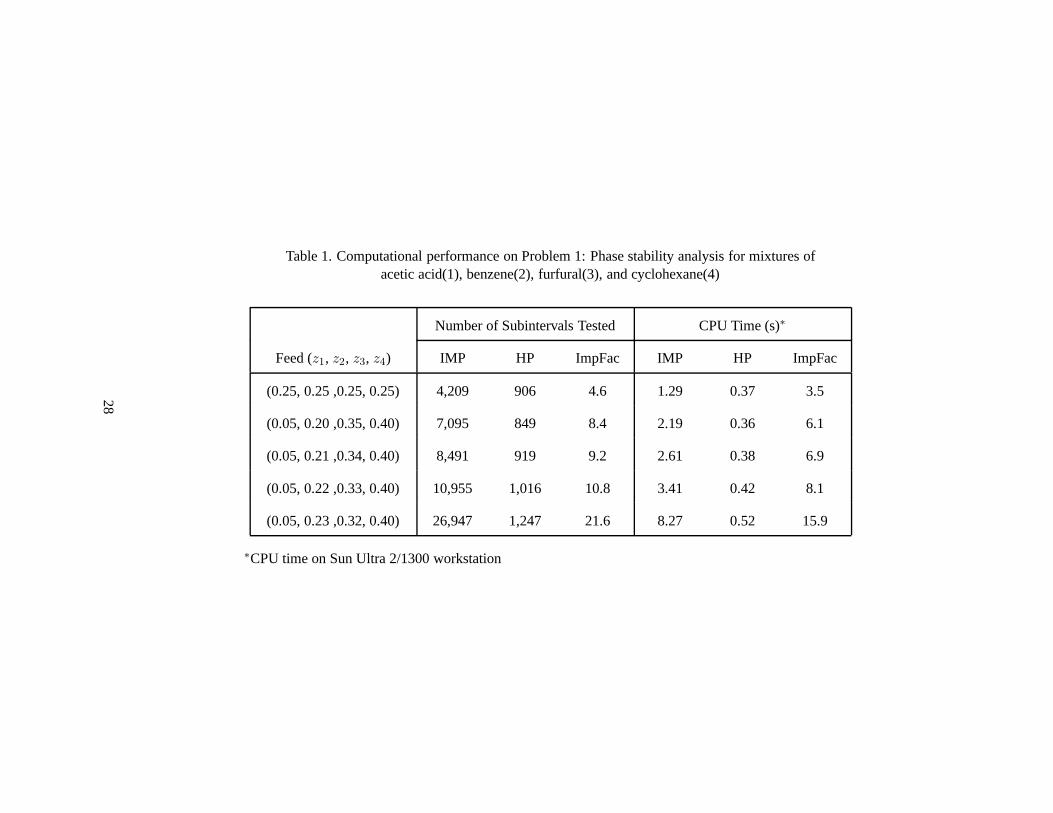
Table 1. Computational performance on Problem 1: Phase stability analysis for mixtures ofacetic acid(1), benzene(2), furfural(3), and cyclohexane(4)

Number of Subintervals Tested CPU Time (s)∗

Feed (z1, z2, z3, z4) IMP HP ImpFac IMP HP ImpFac

(0.25, 0.25 ,0.25, 0.25) 4,209 906 4.6 1.29 0.37 3.5

(0.05, 0.20 ,0.35, 0.40) 7,095 849 8.4 2.19 0.36 6.1

(0.05, 0.21 ,0.34, 0.40) 8,491 919 9.2 2.61 0.38 6.9

(0.05, 0.22 ,0.33, 0.40) 10,955 1,016 10.8 3.41 0.42 8.1

(0.05, 0.23 ,0.32, 0.40) 26,947 1,247 21.6 8.27 0.52 15.9

∗CPU time on Sun Ultra 2/1300 workstation

28

Table 2. Computational performance on Problem 1: Phase stability analysis for mixtures ofacetic acid(1), benzene(2), furfural(3), cyclohexane(4), and water(5)

Number of Subintervals Tested CPU Time (s)∗

Feed (z1, z2, z3, z4, z5) IMP HP ImpFac IMP HP ImpFac

(0.20, 0.20 ,0.20, 0.20, 0.20) 311,745 18,194 17.1 143.68 12.21 11.7

(0.20, 0.25 ,0.20, 0.15, 0.20) 352,054 19,447 18.1 161.25 13.06 12.3

(0.20, 0.25 ,0.25, 0.15, 0.15) 647,875 23,678 27.4 296.40 16.25 18.2

(0.10, 0.25 ,0.25, 0.15, 0.25) 114,753 14,537 7.9 55.28 9.59 5.8

(0.15, 0.25 ,0.25, 0.10, 0.25) 214,395 17,280 12.4 100.63 11.55 8.7

∗CPU time on Sun Ultra 2/1300 workstation

29

Table 3. Computational performance on Problem 1: Phase stability analysis for mixtures ofbenzene(1), cyclohexane(2), 1,2-ethanediol(3), furfural(4), heptane(5), and water(6).

Number of Subintervals Tested CPU Time (s)∗

Feed (z1, z2, z3, z4, z5, z6) IMP HP ImpFac IMP HP ImpFac

(0.10, 0.25 ,0.10, 0.25, 0.10, 0.20)69,567,565 153,876 452.1 50217.3 152.0 330.4

(0.25, 0.10 ,0.10, 0.10, 0.25, 0.20) 9,748,253 122,781 79.4 7077.5 119.9 59.0

(0.10, 0.20 ,0.10, 0.25, 0.25, 0.10)205,932,188 148,331 1388 146903 147.7 994.6

(0.20, 0.10 ,0.10, 0.30, 0.10, 0.20)81,081,374 176,206 460.2 57900.7 176.1 328.8

(0.10, 0.10 ,0.10, 0.20, 0.25, 0.25)68,597,673 118,569 578.5 48986.6 116.4 420.8

∗CPU time on Sun Ultra 2/1300 workstation

30

Table 4. Computational performance on Problem 2: Computation of mixture critical points.

Number of Subintervals Tested CPU Time (s)∗

Mixture IMP HP (ImpFac) HP/RP (ImpFac) IMP HP (ImpFac) HP/RP (ImpFac)

1 405,623 72,157 (5.6) 32,296 (12.6) 154.9 30.8 (5.0) 20.7 (7.5)

2 4,068,420 1,084,110 (3.8) 483,227 (8.4) 2094.1 658.8 (3.2) 406.5 (5.2)

3 7,351,170 3,416,481 (2.2) 2,121,333 (3.4)4909.1 2539.2 (1.9) 1796.2 (2.7)

∗CPU time on Sun Ultra 2/1300 workstation

31

Table 5. Computational performance on Problems 3 and 4: Parameter estimation using EIV approach.

CPU Time (s)∗

Problem IMP HP (ImpFac‡) HP/RP (ImpFac‡)

3 > 172,800† 1504.2 (> 115) 807.9 (> 214)

4 > 172,800† 255.2 (> 677) 28.8 (> 6000)

∗CPU time on Sun Ultra 2/1300 workstation†Program was terminated after 2 CPU days without reaching solution‡Relative to 2 CPU days spent without reaching solution

32