new group iterative schemes in the numerical solution of ... · solution of the two-dimensional...

$: New group iterative schemes in the numerical solution of ... · solution of the two-dimensional time fractional advection-diffusion equation ... Queensland University of ... 2011;$
Balasim & Hj. Mohd. Ali, Cogent Mathematics (2017), 4: 1412241https://doi.org/10.1080/23311835.2017.1412241

COMPUTATIONAL SCIENCE | RESEARCH ARTICLE

New group iterative schemes in the numerical solution of the two-dimensional time fractional advection-diffusion equationAlla Tareq Balasim1,2* and Norhashidah Hj. Mohd. Ali1

Abstarct: Numerical schemes based on small fixed-size grouping strategies have been successfully researched over the last few decades in solving various types of partial differential equations where they have been proven to possess the ability to increase the convergence rates of the iteration processes involved. The formulation of these strategies on fractional differential equations, however, is still at its infancy. Appropriate discretization formula will need to be derived and applied to the time and spatial fractional derivatives in order to reduce the computational complexity of the schemes. In this paper, the design of new group iterative schemes applied to the solution of the 2D time fractional advection-diffusion equation are presented and discussed in detail. The Caputo fractional derivative is used in the discretization of the fractional group schemes in combination with the Crank–Nicolson difference approximations on the standard grid. Numerical experiments are conducted to determine the effectiveness of the proposed group methods with regard to execution times, number of iterations, and computational complexity. The stability and convergence properties are also presented using a matrix method with mathematical induction.The numerical results will be proven to agree with the theoretical claims.

*Corresponding author: Alla Tareq Balasim, School of Mathematical Sciences, Universiti Sains Malaysia, Penang 11800, Malaysia; Department of Mathematics, College of Basic Education, University of Al-mustansiria, Baghdad, IraqE-mail: [email protected]

Reviewing editor:Fawang Liu, Queensland University of Technology, Australia

Additional information is available at the end of the article

ABOUT THE AUTHORSAlla Tareq Balasim is a lecture at the Department of Mathematics Almustansiria University, Iraq. He received his Master in Mathematics from the Department of Mathematics, Baghdad University, Iraq. He is currently a PhD student and his research interests are numerical deferential equations and dynamical system.

Norhashidah Hj. Mohd. Ali is a Professor at the School of Mathematical Sciences, Universiti Sains Malaysia. She received her PhD in Industrial Computing from Universiti Kebangsaan Malaysia. Her areas of expertise include numerical differential equations and parallel numerical algorithms. She has over 25 years teaching and research experiences and has written more than 100 articles in these areas.

PUBLIC INTEREST STATEMENTMany phenomena in science and engineering can be modelled as two dimensional fractional advection-diffusion equations satisfying appropriate initial and boundary conditions. With the advent of computing technology, effective numerical methods have been extensively formulated in solving these equations due to their simplicity and accuracy. In particular, finite difference formulas, are oftenly used to numerically discretize the differential equations to produce sparse systems of linear equations which may be suitably solved by iterative solvers. However, iterative solvers have the disadvantage of being too slow to converge which may increase the computation timings. To overcome this problem, suitable small fixed-size grouping strategies are applied to the mesh points of the solution domain following the discretization of the differential equation which results in schemes with faster convergence and lower computational complexity with comparable accuracies. This is very useful to engineers and scientists who are involved in time consuming simulation modeling processes.

Received: 21 April 2017Accepted: 17 November 2017First Published: 06 December 2017

© 2017 The Author(s). This open access article is distributed under a Creative Commons Attribution (CC-BY) 4.0 license.

Page 1 of 19

http://crossmark.crossref.org/dialog/?doi=10.1080/23311835.2017.1412241&domain=pdf&date_stamp=2017-12-06

mailto:[email protected]

http://creativecommons.org/licenses/by/4.0/

Page 2 of 19


Subjects: Analysis - Mathematics; Applied Mathematics; Computer Mathematics

Keywords: group methods; two-dimensional problem; time fractional advection-diffusion; Caputo fractional derivative; Crank–Nicolson difference schemes; stability & convergence analysis

1. IntroductionFractional calculus, which is the calculus of integrals and derivatives in random order, dates back as far as the more popular integer calculus, and has been gaining significant interest over the past few years with its history and development being explored in detail by Oldham and Spanier (1974), Miller and Ross (1993), Samko, Kilbas, and Marichev (1993) and Podlubny (1998). Fractional differential equations (FDEs) can be used to model many problems in a wide field of applications. They are de-fined as equations that utilize fractional derivatives and considered as powerful tools that can de-scribe the memory and hereditary characteristics of various materials. Several researchers have explored the use of FDEs in the fields of chemistry (Gorenflo, Mainardi, Moretti, Pagnini, & Paradisi, 2002; Seki, Wojcik, & Tachiya, 2003), physics (Henry & Wearne, 2000; Metzler, Barkai, & Klafter, 1999; Metzler & Klafter, 2000; Wyss, 1986) and other scientific and engineering spheres (Baeumer, Benson, Meerschaert, & Wheatcraft, 2001; Benson, Wheatcraft, & Meerschaert, 2000; Cushman & Ginn, 2000; Mehdinejadiani, Naseri, Jafari, Ghanbarzadeh, & Baleanu, 2013). Since there are at most no exact solutions to the majority of fractional differential equations, it is necessary to resort to approxima-tion and numerical methods (Abdelkawy, Zaky, Bhrawy, & Baleanu, 2015; Balasim & Ali, 2015; Baleanu, Agheli, & Al Qurashi, 2016; Bhrawy & Baleanu, 2013). Over the past decade, there has been an influx of numerical methods development for solving various types of FDEs (Agrawal, 2008; Ali, Abdullah, & Mohyud-Din, 2017; Chen, Deng, & Wu, 2013; Chen & Liu, 2008; Chen, Liu, Anh, & Turner, 2011; Chen, Liu, & Burrage, 2008; Leonenko, Meerschaert, & Sikorskii, 2013; Li, Zeng, & Liu, 2012; Liu, Zhuang, Anh, Turner, & Burrage, 2007; Shen, Liu, & Anh, 2011; Sousa & Li, 2015; Su, Wang, & Wang, 2011; Uddin & Haq, 2011; Zhang, Huang, Feng, & Wei, 2013; Zheng, Li, & Zhao, 2010; Zhuang, Gu, Liu, Turner, & Yarlagadda, 2011; Zhuang, Liu, Anh, & Turner, 2009).

Chen et al. (2008) used implicit and explicit difference techniques to solve time fractional reaction-dif-fusion equations, while Liu et al. (2007) proposed for these techniques to be employed in solving the space-time fractional advection-dispersion equation by replacing the first-order time derivative by the Caputo fractional derivative, and the first-order and second-order space derivatives by the Riemman–Liouville fractional derivatives. The use of radial basis function (RBF) approximation method was dis-cussed in Uddin and Haq (2011) to solve the time fractional advection-dispersion equation in a bounded domain. The application of finite element method was also seen in Zheng et al. (2010), in solving the space fractional advection-diffusion equation under non-homogeneous initial boundary conditions. In Chen et al. (2011), a numerical method with first-order temporal accuracy and second-order spatial ac-curacy was established for solving the variable order Galilei advection-diffusion equation with a nonlin-ear source term, while Zhuang et al. (2009) used the explicit and implicit Euler approximation to solve a variable order fractional advection-diffusion equation with a nonlinear source term. A new numerical solution for the 2D fractional advection-dispersion equation with variable coefficients in a finite field was also introduced by Chen and Liu (2008). In 2011, Shen et al. (2011) proposed the explicit and implicit fi-nite difference approximations for the space-time Riesz–Caputo fractional advection-diffusion equation where the implicit scheme was proven to be unconditionally stable, while the explicit scheme exhibits a conditionally stable property. The development of an implicit meshless method was also seen in Zhuang et al. (2011) in solving the time-dependent fractional advection-diffusion equation where a discretized system of equations was obtained using the moving least squares (MLS) meshless shape functions.

In general, finding numerical solutions to FDEs using iterative finite difference schemes is not a straightforward process and can be a challenging task due to several reasons. Firstly, all the earlier solutions have to be saved if the current solution is to be computed, making the calculations even more complex and costly in terms of CPU usage time in cases where traditional point implicit differ-ence approaches are used. Secondly, although the point implicit techniques are stable, a significant

Page 3 of 19


amount of CPU usage time is required when many unknowns are involved. In recent decades, group-ing strategies have been proven to possess characteristics that are able to reduce the spectral radius of the generated matrix resulting from the finite difference discretization of the differential equa-tion, and therefore increase the convergence rates of the iterative algorithms. They have been shown to reduce the computational timings compared to their point wise counterparts in solving several types of partial differential equation (Ali & Kew, 2012; Evans & Yousif, 1986; Kew & Ali, 2015; Ng & Ali, 2008; Othman & Abdullah, 2000; Tan, Ali, & Lai, 2012; Yousif & Evans, 1995). These group methods are also easy to implement and suitable to be implemented on parallel computers due to their explicit nature. However, till date these strategies have not been tested on solving FDEs, par-ticularly for the 2D cases. Therefore, in this study, the formulation of new group iterative methods is presented in solving the following 2Dl time fractional advection diffusion equation

where 0 < 𝛼 < 1, ax, ay , bx, by are positive constants and f(x, y, t) is nonhomogeneous term sub-jected to the following initial and Dirichlet boundary conditions

This equation plays an important role in describing transport dynamics in complex systems which are governed by anomalous diffusion and non-exponential relaxation patterns (Zhuang, Gu, Liu, Turner, & Yarlagadda, 2011). This paper is outlined as follows. Section 2 presents the proposed group iterative methods obtained from the Crank–Nicolson difference approximation followed by the sta-bility and convergence analysis of the difference schemes in Sections 3 and 4, respectively. Section 5 presents the discussion on the computational effort involved in solving Equation (1) using the proposed methods with regard to the arithmetic operations for each iteration. Finally, the results of the numerical experiments are presented and discussed in Section 6.

2. Standard approximation schemes for fractional advection-diffusion equationsThe Caputo fractional derivative, D�, of the order-� is expressed as follows (Li, Qian, & Chen, (2011):

where Γ(⋅) is the Euler Gamma function. Further details on the definitions and properties of frac-tional derivatives are available in Podlubny (1998).

We need to apply appropriate finite difference approximations to the time and space derivaties of (1), let h > 0 be the space step and k > 0 be the time step. The domain is assumed to be uniform in both x and y directions. Define xi = ih, yj = jh, {i, j = 0, 1,...,n}, and a mesh size of h =

1

n, where n is

an arbitrary positive integer and tk = k�, k = 0, 1,..., l. various approximations formulas could be obtained for (1) at the point of (xi , yj , tk). By taking the average of the central difference approxima-tions to the left side of (1) at the points (i, j, k + 1) and (i, j, k), the Caputo time fractional approxi-mation (2) can be transformed to the following form (Karatay, Kale, & Bayramoglu, 2013)

where � =1

�� Γ(2−�)

, ws = �((s + 1

2)1−�

− (s − 1

2)1−�

).

Using (3) in combination with the second-order Crank–Nicolson difference scheme for the right side of (1) will result in the following fractional standard point (FSP) formula

(1)��u

�t�= ax

�2u

�x2+ ay

�2u

�y2− bx

�u

�x− by

�u

�y+ f (x, y, t),

u(x, y, 0) = g(x, y)

u(0, y, t) = g1(y, t) u(1, y, t) = g2(y, t)

u(x, 0, t) = g3(x, t) u(x, 1, t) = g4(x, t)

(2)D𝛼 =1

Γ(m − 𝛼)

x

∫0

f m(t)

(x − t)𝛼−m+1dt, 𝛼 > 0, m − 1 < 𝛼 < m, m ∈ N, x > 0,

(3)

��u(xi ,yj ,tk+1)

�t�= w1u

k +∑k−1

s=1

�wk−s+1 −wk−s

�usi,j −wku

0i, j + �

(uk+1i,j −uki,j)21−�

+O(�2−�),

Page 4 of 19


Equation (4) can be simplified to become as follows

(4)

w1uk +

∑k−1

s=1


�usi,j −wku

0

i, j + �(uk+1i,j −uki,j)

21−�

=ax

2

�uk+1i−1,j−2u

k+1i,j +uk+1i+1,j

h2+

uki−1,j−2uki,j+u

ki+1,j

h2

�

+ay

2

�uk+1i,j−1−2u

k+1i,j +uk+1i,j+1

h2+

uki,j−1−2uki,j+u

ki,j+1

h2

�−

bx

2

�uk+1i+1,j−u

k+1i−1,j

2h+

uki+1,j−uki−1,j

2h

�

−by

2

�uk+1i,j+1−u

k+1i,j−1

2h+

uki,j+1−uki,j−1

2h

�+ f

k+ 1

2

i, j+ O(�2−� + (△x)

2+ (△y)

2).

(5)

�1 + sx + sy

�uk+1i,j = (

sx

2+

cx

4)uk+1i−1,j + (

sx

2−

cx

4)uk+1i+1,j + (

sy

2+

cy

4)uk+1i,j−1

+(sy

2−

cy

4)uk+1i,j+1 +

�1 − 21−�w∗

1− sx − sy

�uki,j + (

sx

2+

cx

4)uki−1,j

+(sx

2−

cx

4)uki+1,j + (

sy

2+

cy

4)uki,j−1 + (

sy

2−

cy

4)uki,j+1 + 2

1−�w∗

ku0

i,j

+21−�∑k−1

s=1

�w∗

k−s −w∗

k−s+1

�usi,j +m0

fk+1∕2

i,j

Figure 1. Computational molecule of the standard point approximation.

1-w1-sx-sy

(w1-w2)

(w2-w3)

(wk-1-wk)

wk

. . .

i,j-1,k

Time level

k

i,j,k

i,j,k-1

.

. i,j,1

i, j-1,k+1

i-1,j,k+1i,j,k+1

i+1,j,k

Time level

1

Time level

0

i,j,0

Time level

k+1

i,j+1,k+1

i+1,j,k+1

i-1,j,k

Time level

k-1

Time level

k-2

i,j,k-2

i+1,j,k

1+sx+sy1+sx+sx y

1-w1-sx-sy

sx/2+cx/4

sy/2-cy/4

sx/2-cx/4

sy/2+cy/4

sx/2+cx/4

sy/2+cy/4

sy/2-cy/4

sx/2-cx/4

(w1-w2)

(w2-w3)

(wk-1-wk)

wk

Page 5 of 19


where m0 = 21−� t� Γ(2 − �), w∗

s =((s + 1∕2)1−� − (s − 1∕2)1−�

), sx =

ax m0

h2, sy =

ay m0

h2, cx =

bx m0

h, cy =

by m0

h.

Figure 1 shows the computational molecule for Equation (5).

2.1. Fractional explicit group methodIn formulating the fractional explicit group (FEG) method, (5) is applied to any group of four points in the solution domain to generate a 4 × 4 system of equation as follows

where D = 1 + sx + sy , a1 =(sx

2−

cx

4

), b1 =

(sy

2−

cy

4

), a2 =

(sx

2+

cx

4

), b2 =

(sy

2+

cy

4

),

R = (1 − 21−�w∗

1 − sx − sy),

Mathematical software can be used to easily invert (6) to obtain the FEG formula

(6)

⎛⎜⎜⎜⎜⎝

D −a1 0 −b1−a2 D −b1 0

0 −b2 D −a2−b2 0 −a1 D

⎞⎟⎟⎟⎟⎠

⎛⎜⎜⎜⎜⎝

ui,jui+1,jui+1,j+1ui,j+1

⎞⎟⎟⎟⎟⎠=

⎛⎜⎜⎜⎜⎝

rhsi,jrhsi+1,jrhsi+1,j+1rhsi,j+1

⎞⎟⎟⎟⎟⎠,

rhsi,j =a2(uk+1i−1,j + u

ki−1,j) + b2(u

k+1i,j−1 + u

ki,j−1) + a1u

ki+1,j + b1u

ki,j+1

+ 21−�w∗

ku0i,j + Ru

ki,j +

k−1∑s=1

21−�[w∗

k−s −w∗

k−s+1]usi.j +m0f

k+1∕2

i,j,

rhsi+1,j =a1(uk+1i+2,j + u

ki+2,j) + b2(u

k+1i+1,j−1 + u

ki+1,j−1) + b1u

ki+1,j+1 + a2u

ki,j

+ 21−�w∗

ku0i+1,j + Ru

ki+1,j +

k−1∑s=1

21−�[w∗

k−s −w∗

k−s+1]usi+1,j +m0f

k+1∕2

i+1,j,

rhsi+1,j+1 =a1(uk+1i+2,j+1 + u

ki+2,j+1) + b1(u

k+1i+1,j+2 + u

ki+1,j+2) + b2u

ki+1,j + a2u

ki,j+1

+ 21−�w∗

ku0i+1,j+1 + Ru

ki+1,j+1 +

k−1∑s=1

21−�[w∗

k−s −w∗

k−s+1]usi+1,j+1 +m0f

k+1∕2

i+1,j+1,

rhsi,j+1 =a2(uk+1i−1,j+1 + u

ki−1,j+1) + b1(u

k+1i,j+2 + u

ki,j+2) + a1u

ki+1,j+1 + b2u

ki,j

+ 21−�w∗

ku0i,j+1 + Ru

ki,j+1 +

k−1∑s=1

21−�[w∗

k−s −w∗

k−s+1]usi,j+1 +m0f

k+1∕2

i,j+1.

Figure 2. Grouping of the points for the FEG method (n = 10).

Page 6 of 19


where

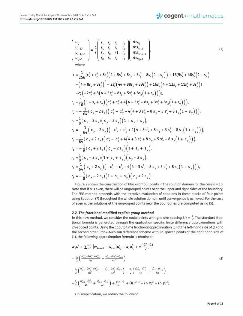
Figure 2 shows the construction of blocks of four points in the solution domain for the case n = 10. Note that if n is even, there will be ungrouped points near the upper and right sides of the boundary. The FEG method proceeds with the iterative evaluation of solutions in these blocks of four points using Equation (7) throughout the whole solution domain until convergence is achieved. For the case of even n, the solutions at the ungrouped points near the boundaries are computed using (5).

2.2. The fractional modified explicit group methodIn this new method, we consider the nodal points with grid size spacing 2h =

2

n. The standard frac-

tional formula is generated through the application specific finite difference approximations with 2h-spaced points. Using the Caputo time fractional approximation (3) at the left-hand side of (1) and the second order Crank–Nicolson difference scheme with 2h-spaced points at the right hand side of (1), the following approximation formula is obtained:

On simplification, we obtain the following

(7)

⎛⎜⎜⎜⎜⎝


⎞⎟⎟⎟⎟⎠=1

r

⎛⎜⎜⎜⎜⎝

r1 r2 r3 r4r5 r1 r4 r6r7 r8 r1 r5r8 r9 r2 r1

⎞⎟⎟⎟⎟⎠

⎛⎜⎜⎜⎜⎝


⎞⎟⎟⎟⎟⎠,

r =1

256(c4x+ c4

y+ 8c2

y

(4 + 5s2

x+ 8s

y+ 3s2

y+ 8s

x

(1 + s

y

))+ 16[9s4

x+ 48s3

x

(1 + s

y

)

+(4 + 8s

y+ 3s2

y

)2+ 2s2

x

(44 + 88s

y+ 39s2

y

)+ 16s

x

(4 + 12s

y+ 11s2

y+ 3s3

y

)]

+c2x

(−2c2

y+ 8

(4 + 3s2

x+ 8s

y+ 5s2

y+ 8s

x

(1 + s

y

)))),

r1=1

16

(1 + s

x+ s

y

)(c2x+ c2

y+ 4

(4 + 3s2

x+ 8s

y+ 3s2

y+ 8s

x

(1 + s

y

))),

r2= −

1

64

(cx− 2 s

x

)(c2x− c2

y+ 4

(4 + 3 s2

x+ 8 s

y+ 5 s2

y+ 8 s

x

(1 + s

y

))),

r3=1

8

(cx− 2 s

x

)(cy− 2 s

y

)(1 + s

x+ s

y

),

r4= −

1

64

(cy− 2 s

y

)(− c2

x+ c2

y+ 4

(4 + 5 s2

x+ 8 s

y+ 3 s2

y+ 8 s

x

(1 + s

y

))),

r5=1

64

(cx+ 2 s

x

)(c2x− c2

y+ 4

(4 + 3 s2

x+ 8 s

y+ 5 s2

y+ 8 s

x

(1 + s

y

))),

r6= −

1

8

(cx+ 2 s

x

)(cy− 2 s

y

)(1 + s

x+ s

y

),

r7=1

8

(cx+ 2 s

x

)(1 + s

x+ s

y

)(cy+ 2 s

y

),

r8=1

64

(cy+ 2 s

y

)(− c2

x+ c2

y+ 4

(4 + 5 s2

x+ 8 s

y+ 3 s2

y+ 8 s

x

(1 + s

y

))),

r9= −

1

8

(cx− 2 s

x

)(1 + s

x+ s

y

)(cy+ 2 s

y

).

(8)

w1uk +

∑k−1

s=1


�usi,j −wku

0

i, j + �(uk+1i,j −uki,j)

21−�

=ax

2

�uk+1i−2,j−2u

k+1i,j +uk+1i+2,j

4h2 +

uki−2,j−2uki,j+u

ki+2,j

4h2

�

+ay

2

�uk+1i,j−2−2u

k+1i,j +uk+1i,j+2

4h2 +

uki,j−2−2uki,j+u

ki,j+2

4h2

�−

bx

2

�uk+1i+2,j−u

k+1i−2,j

4h+

uki+2,j−uki−2,j

4h

�

−by

2

�uk+1i,j+2−u

k+1i,j−2

4h+

uki,j+2−uki,j−2

4h

�+ f

k+1∕2

i, j+ O(�2−� + (▵ x)2 + (▵ y)2).

Page 7 of 19


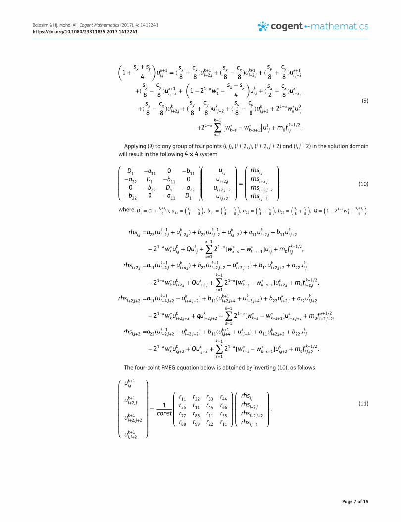
Applying (9) to any group of four points (i, j), (i + 2, j), (i + 2, j + 2) and (i, j + 2) in the solution domain will result in the following 4 × 4 system

where, D1 = (1 +sx+sy

4), a11 =

(sx

8−

cx

8

), b11 =

(sy

8−

cy

8

), a22 =

(sx

8+

cx

8

), b22 =

(sy

8+

cy

8

), Q =

(1 − 21−�w∗

1 −sx+sy

4

),

The four-point FMEG equation below is obtained by inverting (10), as follows

(9)

(1 +

sx + sy

4

)uk+1i,j = (

sx8

+cx8)uk+1i−2,j + (

sx8

−cx8)uk+1i+2,j + (

sy

8+cy

8)uk+1i,j−2

+(sy

8−cy

8)uk+1i,j+2 +

(1 − 21−�w∗

1 −sx + sy

4

)uki,j + (

sx2

+cx8)uki−2,j

+(sx8

−cx8)uki+2,j + (

sy

8+cy

8)uki,j−2 + (

sy

8−cy

8)uki,j+2 + 2

1−�w∗

ku0i,j

+21−�k−1∑s=1

[w∗

k−s −w∗

k−s+1

]usi,j +m0f

k+1∕2

i,j.

(10)

⎛⎜⎜⎜⎜⎝

D1 −a11 0 −b11−a22 D1 −b11 0

0 −b22 D1 −a22−b22 0 −a11 D1

⎞⎟⎟⎟⎟⎠

⎛⎜⎜⎜⎜⎝


⎞⎟⎟⎟⎟⎠=

⎛⎜⎜⎜⎜⎝


⎞⎟⎟⎟⎟⎠,

rhsi,j =a22(uk+1i−2,j + u

ki−2,j) + b22(u

k+1i,j−2 + u

ki,j−2) + a11u

ki+2,j + b11u

ki,j+2

+ 21−�w∗

ku0i,j + Qu

ki,j +

k−1∑s=1

21−�[w∗

k−s −w∗

k−s+1]usi.j +m0f

k+1∕2

i,j,

rhsi+2,j =a11(uk+1i+4,j + u

ki+4,j) + b22(u

k+1i+2,j−2 + u

ki+2,j−2) + b11u

ki+2,j+2 + a22u

ki,j

+ 21−�w∗

ku0i+2,j + Qu

ki+2,j +

k−1∑s=1

21−�[w∗

k−s −w∗

k−s+1]usi+2,j +m0f

k+1∕2

i+2,j,

rhsi+2,j+2 =a11(uk+1i+4,j+2 + u

ki+4,j+2) + b11(u

k+1i+2,j+4 + u

ki+2,j+4) + b22u

ki+2,j + a22u

ki,j+2

+ 21−�w∗

ku0i+2,j+2 + qu

ki+2,j+2 +

k−1∑s=1

21−�[w∗

k−s −w∗

k−s+1]usi+2,j+2 +m0f

k+1∕2

i+2,j+2,

rhsi,j+2 =a22(uk+1i−2,j+2 + u

ki−2,j+2) + b11(u

k+1i,j+4 + u

ki,j+4) + a11u

ki+2,j+2 + b22u

ki,j

+ 21−�w∗

ku0i,j+2 + Qu

ki,j+2 +

k−1∑s=1

21−�[w∗

k−s −w∗

k−s+1]usi,j+2 +m0f

k+1∕2

i,j+2.

(11)

⎛⎜⎜⎜⎜⎜⎜⎜⎜⎝

uk+1i.j

uk+1i+2, j

uk+1i+2, j+2

uk+1i, j+2

⎞⎟⎟⎟⎟⎟⎟⎟⎟⎠

=1

const

⎛⎜⎜⎜⎜⎝

r11

r22

r33

r44

r55

r11

r44

r66

r77

r88

r11

r55

r88

r99

r22

r11

⎞⎟⎟⎟⎟⎠

⎛⎜⎜⎜⎜⎝


⎞⎟⎟⎟⎟⎠,

Page 8 of 19


To use this method, the grid points in the solution domain are divided into three types of points, denoted by the symbols ✷,△ and ∙ in alternate ordering as shown in Figure 3. Note that the evalu-ation of (11) require points of type ∙ only. Thus, we can construct the FMEG method by generating the iterations on this type of points only, followed by the evaluation of solutions directly once on points of type ✷ and △ . The FMEG algorithm can then be summarized as follows:

(1) Divide the grid points into three types ✷,△ and ∙ in alternate order as depicted in Figure 3.

(2) Set the initial guess for the iterations.

cons =1

4096(4096 + c4

x+ c4

y+ 4096s

x+ 1408s2

x+ 192s3

x+ 9s4

x+ 4096s

y

+3072sxsy+ 704s2

xsy+ 48s3

xsy+ 1408s2

y+ 704s

xs2y+ 78s2

xs2y+ 192s3

y

+48sxs3y+ 9s4

y+ 2c2

y

(64 + 5s2

x+ 32s

y+ 3s2

y+ 8s

x

(4 + s

y

))

+2c2x

(64 − c2

y+ 3s2

x+ 32s

y+ 5s2

y+ 8s

x

(4 + s

y

))),

r11

=1

256

(4 + s

x+ s

y

)(64 + c2

x+ c2

y+ 32s

x+ 3s2

x+ 32s

y+ 8s

xsy+ 3s2

y

),

r22

= −1

512

(cx− s

x

)(64 + c2

x− c2

y+ 32s

x+ 3s2

x+ 32s

y+ 8s

xsy+ 5s2

y

),

r33

= −1

512

(cx− s

x

)(64 + c2

x− c2

y+ 32s

x+ 3s2

x+ 32s

y+ 8s

xsy+ 5s2

y

),

r44

= −1

512

(cy− s

y

)(64 − c2

x+ c2

y+ 32s

x+ 5s2

x+ 32s

y+ 8s

xsy+ 3s2

y

),

r55

=1

512

(cx+ s

x

)(64 + c2

x− c2

y+ 32s

x+ 3s2

x+ 32s

y+ 8s

xsy+ 5s2

y

),

r66

= −1

128

(cx+ s

x

)(cy− s

y

)(4 + s

x+ s

y

),

r77

=1

128

(cx+ s

x

)(cy+ s

y

)(4 + s

x+ s

y

),

r88 =1

512

(cy + sy

)(64 − c2x + c

2y + 32sx + 5s

2x + 32sy + 8sxsy + 3s

2y

),

r99 = −1

128

(cx − sx

)(cy + sy

)(4 + sx + sy

).

Figure 3. Grouping of the points for the FMEG method (n = 10).

0 1 2 3 4 5 6 7 8 9 10

Page 9 of 19


(3) Evaluate the solutions at points ∙ using Equation (11) iteratively at the time level k + 1.

(4) Step 5 is performed if the iteration converges. Otherwise, Step 3 is repeated until a conver-gence is attained.

(5) The steps below are performed directly once for points ✷ and △ in Figure 3 at the time level k + 1:

(a) For type ✷ points, the rotated h − spaced five-point approximation formula derived by rotating the x − y axis clockwise at 45o was used (Tan, Ali, & Lai, 2012). This approxima-tion formula was applied to the right side of Equation (1), in combination with (3) being applied to the left side of (1), to obtain the following rotated C-N formula:

(b) For type △ points, the typical h − spaced formula (5) is used. Note that formula (5) involve points of type △ only.

3. Stability analysisA scheme is considered to be stable if the errors cease to increase with the passing of time, and gradually become inconsequential as the computation progresses. Even though the spacing is dif-ferent, Equation (5) gives rise to both the FEG and FMEG methods. Therefore, the stability of both methods can be analyzed in similar ways. Here, we will show the stability of the FMEG scheme using eigenvalues of the generated matrices with mathematical induction.

Form (10) we obtain

where A =

⎛⎜⎜⎜⎜⎜⎝

R1 R2 0 0

R3 R1 R2 0

⋱

0 R3 R1 R20 0 R3 R1

⎞⎟⎟⎟⎟⎟⎠

, B =

⎛⎜⎜⎜⎜⎜⎝

S1 S2 0 0

S3 S1 S2 0

⋱

0 S3 S1 S20 0 S3 S1

⎞⎟⎟⎟⎟⎟⎠

, b =

⎛⎜⎜⎜⎜⎜⎝

W1

W1

⋮

W1

W1

⎞⎟⎟⎟⎟⎟⎠

R1 =

⎛⎜⎜⎜⎜⎜⎝

G1 G3G2 G1 G3

⋱

G2 G1 G3G2 G1

⎞⎟⎟⎟⎟⎟⎠

R2 =

⎛⎜⎜⎜⎜⎜⎝

G5G5

⋱

G5G5

⎞⎟⎟⎟⎟⎟⎠

R3 =

⎛⎜⎜⎜⎜⎜⎝

G4G4

⋱

G4G4

⎞⎟⎟⎟⎟⎟⎠

,

(1 +

sx + sy

2

)uk+1i,j = (

sx4

+cx − cy

8)uk+1i−1,j+1 + (

sx4

−cx + cy

8)uk+1i+1,j+1 + (

sy

4+cy − cx

8)uk+1i+1,j−1

+ (sy

4+cx + cy

8)uk+1i−1,j−1 +

(1 − 21−�w∗

1 −sx + sy

2

)uki,j + (

sx4

+cx − cy

8)uki−1,j+1

+ (sx4

−cx + cy

8)uki+1,j+1 + (

sy

4+cy − cx

8)uki+1,j−1 + (

sy

4+cx + cy

8)uki−1,j−1 + 2

1−�w∗

ku0i,j

+ 21−�k−1∑s=1

[w∗

k−s −w∗

k−s+1

]usi,j +m0f

k+1∕2

i,j.

(12)

AU1 = BU k = 0

AUk+1 = BUk − C1Uk +

∑k−1

s=1Ck−sUs + C

kUo + b k > 0

Page 10 of 19


S1 =

⎛⎜⎜⎜⎜⎜⎝

H1 H3H2 H1 H3

⋱

H2 H1 H3H2 H1

⎞⎟⎟⎟⎟⎟⎠

S2 =

⎛⎜⎜⎜⎜⎜⎝

H5H5

⋱

H5H5

⎞⎟⎟⎟⎟⎟⎠

S3 =

⎛⎜⎜⎜⎜⎜⎝

H4H4

⋱

H4H4

⎞⎟⎟⎟⎟⎟⎠

Ck =

⎛⎜⎜⎜⎜⎜⎝

Mk

Mk

⋱

Mk

Mk

⎞⎟⎟⎟⎟⎟⎠

Ck−s =

⎛⎜⎜⎜⎜⎜⎝

Mk−s

Mk−s

⋱

Mk−s

Mk−s

⎞⎟⎟⎟⎟⎟⎠

, s = 1, ..., k − 1

C1 =

⎛⎜⎜⎜⎜⎜⎝

M1

M1

⋱

M1

M1

⎞⎟⎟⎟⎟⎟⎠

, W1 =

⎛⎜⎜⎜⎜⎜⎝

L1L1⋮

L1L1

⎞⎟⎟⎟⎟⎟⎠

, G1 =

⎛⎜⎜⎜⎜⎝

D1 −a11 0 −b11−a22 D1 −b11 0

0 −b22 D1 −a22−b22 0 −a11 D1

⎞⎟⎟⎟⎟⎠

G2 =

⎛⎜⎜⎜⎜⎝

0 0 0 −b220 0 −b22 0

0 0 0 0

0 0 0 0

⎞⎟⎟⎟⎟⎠, G3 =

⎛⎜⎜⎜⎜⎝

0 0 0 0

0 0 0 0

0 −b11 0 0

−b11 0 0 0

⎞⎟⎟⎟⎟⎠G4 =

⎛⎜⎜⎜⎜⎝

0 −a22 0 0

0 0 0 0

0 0 0 0

0 0 −a22 0

⎞⎟⎟⎟⎟⎠,

G5 =

⎛⎜⎜⎜⎜⎝

0 0 0 0

−a11 0 0 0

0 0 0 −a110 0 0 0

⎞⎟⎟⎟⎟⎠, H1 =

⎛⎜⎜⎜⎜⎝

Q a11 0 b11a22 Q b11 0

0 b22 Q a22b22 0 a11 Q

⎞⎟⎟⎟⎟⎠, H2 =

⎛⎜⎜⎜⎜⎝

0 0 0 b220 0 b22 0

0 0 0 0

0 0 0 0

⎞⎟⎟⎟⎟⎠

H3 =

⎛⎜⎜⎜⎜⎝

0 0 0 0

0 0 0 0

0 b11 0 0

b11 0 0 0

⎞⎟⎟⎟⎟⎠, H4 =

⎛⎜⎜⎜⎜⎝

0 a22 0 0

0 0 0 0

0 0 0 0

0 0 a22 0

⎞⎟⎟⎟⎟⎠, H5 =

⎛⎜⎜⎜⎜⎝

0 0 0 0

a11 0 0 0

0 0 0 a110 0 0 0

⎞⎟⎟⎟⎟⎠

Mk−s =21−�

t�

⎛⎜⎜⎜⎜⎝

(w∗

k−s−w∗

k−s+1) 0 0 0

0 (w∗

k−s−w∗

k−s+1) 0 0

0 0 (w∗

k−s−w∗

k−s+1) 0

0 0 0 (w∗

k−s−w∗

k−s+1)

⎞⎟⎟⎟⎟⎠,

M1 =21−�

t�

⎛⎜⎜⎜⎜⎝

w∗

10 0 0

0 w∗

10 0

0 0 w∗

10

0 0 0 w∗

1

⎞⎟⎟⎟⎟⎠, Mk =

21−�

t�

⎛⎜⎜⎜⎜⎝

w∗

k0 0 0

0 w∗

k0 0

0 0 w∗

k0

0 0 0 w∗

k

⎞⎟⎟⎟⎟⎠,

L1 = 21−�Γ[2 − �]

⎛⎜⎜⎜⎜⎝

fi,jfi+2,jfi+2,j+2fi,j+2

⎞⎟⎟⎟⎟⎠, i, j = 2, 6, ...,n − 2.

Page 11 of 19


The following lemma is important to prove the stability.

Lemma 1 [Karatay, Kale, & Bayramoglu, 2013] In (12), the coefficients w∗

s , s = 1, 2, ..., k satisfy the fol-lowing 1 −w∗

k−s > w∗

k−s+1, s = 1, 2, ..., k. 2 −∑k−1

S=1 [w∗

k−s −w∗

k−s+1] +w∗

k = w∗

1, s = 1, 2, ..., k.

For simplicity, we assume sx = sy = S =Γ(2−�)2

1−�

h2, cx = cy = C =

Γ(2−�)21−�

h,D

1=

1

t�+

S

2 and

Q =1

t�− 21−�w∗

1−

S

2

Theorem 1 If �

1

t𝛼−

S

2−

21−𝛼

t𝛼w∗

1+

√−C2+S2

4

�> 0 then the FMEG scheme (10) is stable.

Proof To prove the stability of (10), we suppose that uki,j , i, j = 1, 2, ...,n, k = 1, 2, ..., l are the ap-proximate solutions to the exact solution Uki,j of (1), the error �ki,j = U

ki,j − u

ki,j be the error at time level

k. From (12), the error satisfies

where

Ek+1 =

⎛⎜⎜⎜⎜⎜⎝

Ek+11

Ek+11

⋮

Ek+11

Ek+11

⎞⎟⎟⎟⎟⎟⎠

, Ek+11 =

⎛⎜⎜⎜⎜⎜⎝

�k+12

�k+14

⋮

�k+1m−4

�k+1m−2

⎞⎟⎟⎟⎟⎟⎠

, �k+1i =

⎡⎢⎢⎢⎢⎣

�k+1i,j

�k+1i+2,j

�k+1i+2,j+2

�k+1i,j+2

⎤⎥⎥⎥⎥⎦, i = 2, 6, ...,n − 2, j = 2, 6, ..., n − 2

.

From the above equations, the following are obtained:

It is worthy to note that, from (14), the eigenvalues of the matrices A,B,C1,Ck−s and Ck are ak, bk, c1, ck−s and ck respectively, where

(13)AE1 = BE k = 0

AEk+1 = BEk − C1Ek +

∑k−1

s=1 Ck−sUs + CkE

o k > 0

(14)

A = G4 + G2 + G1 + G3 + G5B = H4 + H2 + H1 + H3 + H5C1 = M1

Ck−s = Mk−s

Ck = Mk

Table 1. Number of various types of mesh points for the point and explicit group methodsPoint types Number of points

FSP FEG FMEGIterative group points m

2 (m − 1)2 (m−1)2

4

Iterative ungrouped points – 2m-1 –

Total iterative points m2

m2

(m−1)2

4

Direct h-spaced rotated points – – (m+1)2

4

Direct h-spaced standard points – – m2−1

4

Total direct points – – 3m2+2m−1

4

Page 12 of 19


For k = 0

Supposing that: ‖‖Es‖‖ ≤ ‖‖‖E0‖‖‖, s = 1, ..., k.

Need to prove this inequality holds for s = k + 1.

Using Lemma 1, we get

Therefore, under the conditions �1

t𝛼−

S

2−

21−𝛼

t𝛼w∗

1 +

√−C2+S2

4

�> 0 the FMEG iterative scheme (10)

is stable. ✷

ak =

�1

t�+S

2,1

t�+S

2,1

4

�4

t�+ 2S −

√−C2 + S2

�,1

4

�4

t�+ 2S +

√−C2 + S2

��

bk =

�1

t�−S

2,1

t�−S

2,1

4

�4

t�− 2S −

√−C2 + S2

�,1

4

�4

t�− 2S +

√−C2 + S2

��

c1 =21−�

t�w∗

1

ck−s =21−�

t�(w∗

k−s −w∗

k−s+1)

ck =21−�

t�w∗

k

E1 = A−1 B E0

��E1�� ≤ �(A−1B)

��E0�� =

��

�1

t�−

S

2+

√−C2+S2

4

��1

t�+

S

2+

√−C2+S2

4

��

��E0��

∴��E

1�� ≤ ��E0��

Ek+1 = A−1(B − C1)Ek +

k−1∑s=1

A−1Ck−sEs + A−1CkE

0

≤ �(A−1(B − C1))‖‖‖E

0‖‖‖ +k−1∑s=1

�(A−1Ck−s)‖‖‖E

0‖‖‖ + �(A−1Ck)‖‖‖E

0‖‖‖

��Ek+1�� ≤

��1

t�−

S

2−

21−�

t�w∗

1 +

√−C2+S2

4

��1

t�+

S

2+

√−C2+S2

4

� ��E0�� +

21−�

t�w∗

1�1

t�+

S

2+

√−C2+S2

4

��E0��

∴��E

k+1�� ≤ ��E0��

Table 2. Computational complexity for the point and explicit group methodsPer iteration After convergence

Methods Additional Multiplication Additional MultiplicationSFP (14 + 13(k − 1))m2 (10 + (k − 1))m2 – –

FEG (15 + 13(k − 1))(m − 1)2 + (14 + 13(k − 1))(2m − 1) (14 + (k − 1))(m − 1)2 + (10 + (k − 1))(2m − 1) – –

FMEG ((15+13(k−1))(m−1)2)

4

((14+(k−1))(m−1)2)

4

(14 + 13(k − 1)) ×(3m

2+2m−1)

4(10 + (k − 1)) ×

(3m2+2m−1)

4

Page 13 of 19


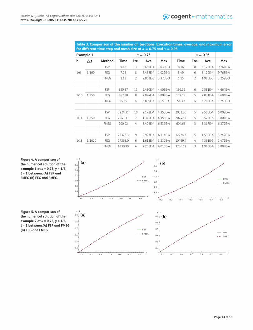
Table 3. Comparison of the number of iterations, Execution times, average, and maximum error for different time step and mesh size at � = 0.75 and � = 0.95

Example 1 � = 0.75 � = 0.95

h △t Method Time Ite. Ave Max Time Ite. Ave MaxFSP 9.18 11 6.485E-4 1.030E-3 6.16 8 6.125E-4 9.761E-4

1/6 1/100 FEG 7.25 8 6.458E-4 1.029E-3 5.49 6 6.120E-4 9.763E-4

FMEG 1.13 2 2.063E-3 3.375E-3 1.15 2 1.986E-3 3.252E-3

FSP 350.37 11 2.480E-4 4.409E-4 195.31 6 2.581E-4 4.664E-4

1/10 1/350 FEG 367.80 8 2.094E-4 3.807E-4 172.19 5 2.031E-4 3.681E-4

FMEG 54.55 4 6.899E-4 1.27E-3 54.30 4 6.709E-4 1.240E-3

FSP 3924.31 10 2.172E-4 4.353E-4 2032.86 5 2.506E-4 5.002E-4

1/14 1/850 FEG 2941.31 7 1.346E-4 4.353E-4 2024.52 5 9.522E-5 1.801E-4

FMEG 700.02 4 3.402E-4 6.539E-4 604.66 3 3.317E-4 6.372E-4

FSP 22323.3 9 2.923E-4 6.114E-4 12224.3 5 1.599E-4 3.242E-4

1/18 1/1620 FEG 17268.0 6 1.613E-4 3.212E-4 10499.4 4 7.361E-5 1.471E-4

FMEG 4330.99 4 2.208E-4 4.015E-4 3786.52 3 1.966E-4 3.887E-4

Figure 4. A comparison of the numerical solution of the example 1 at � = 0.75, y = 1/6, t = 1 between, (A) FSP and FMEG (B) FEG and FMEG.

:

:

:

:

::

:

:

:

:

:(a) (b)

Figure 5. A comparison of the numerical solution of the example 2 at � = 0.75, y = 1/6, t = 1 between,(A) FSP and FMEG (B) FEG and FMEG.

::

::

:

:

:

:

:

:

:

:(a) (b)

Page 14 of 19


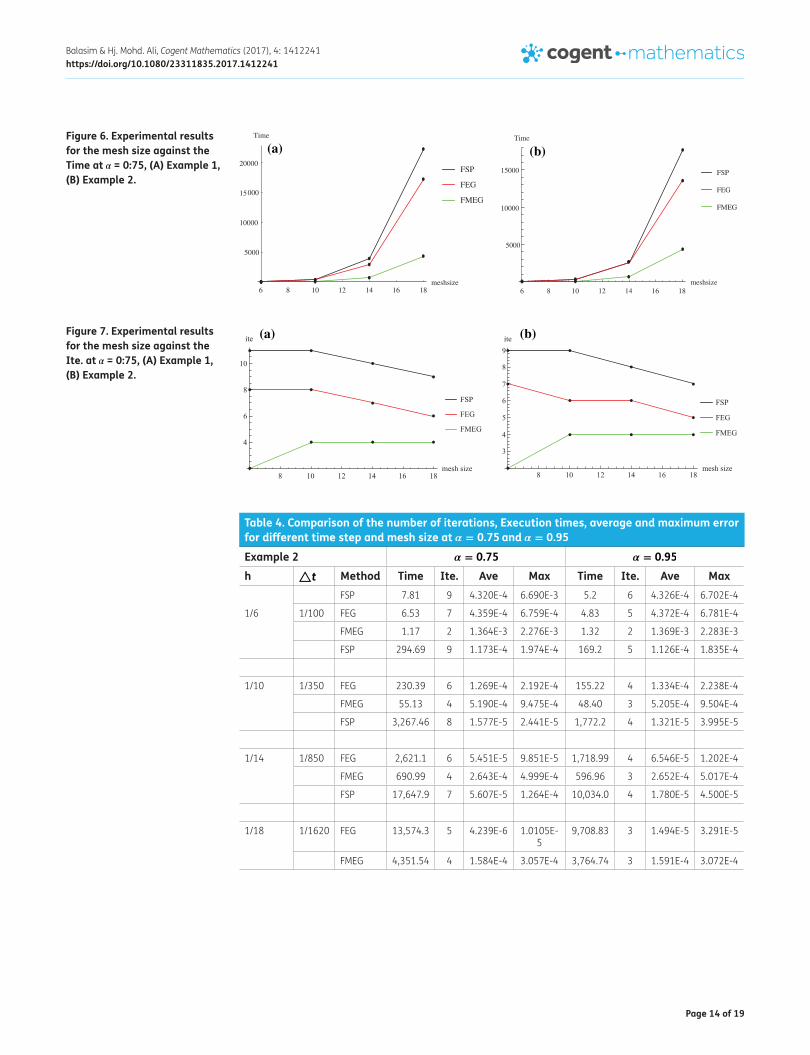
Figure 6. Experimental results for the mesh size against the Time at � = 0:75, (A) Example 1, (B) Example 2.

6 8 10 12 14 16 18meshsize

5000

10000

15000

20000

Time

FSP

FEG

FMEG

6 8 10 12 14 16 18meshsize

5000

10000

15000

Time

FSP

FEG

FMEG

(a) (b)

Figure 7. Experimental results for the mesh size against the Ite. at � = 0:75, (A) Example 1, (B) Example 2.

8 10 12 14 16 18mesh size

4

6

8

10

ite

FSP

FEG

FMEG

8 10 12 14 16 18mesh size

3

4

5

6

7

8

9ite

FSP

FEG

FMEG

(a) (b)

Table 4. Comparison of the number of iterations, Execution times, average and maximum error for different time step and mesh size at � = 0.75 and � = 0.95

Example 2 � = 0.75 � = 0.95

h △t Method Time Ite. Ave Max Time Ite. Ave MaxFSP 7.81 9 4.320E-4 6.690E-3 5.2 6 4.326E-4 6.702E-4

1/6 1/100 FEG 6.53 7 4.359E-4 6.759E-4 4.83 5 4.372E-4 6.781E-4

FMEG 1.17 2 1.364E-3 2.276E-3 1.32 2 1.369E-3 2.283E-3

FSP 294.69 9 1.173E-4 1.974E-4 169.2 5 1.126E-4 1.835E-4

1/10 1/350 FEG 230.39 6 1.269E-4 2.192E-4 155.22 4 1.334E-4 2.238E-4

FMEG 55.13 4 5.190E-4 9.475E-4 48.40 3 5.205E-4 9.504E-4

FSP 3,267.46 8 1.577E-5 2.441E-5 1,772.2 4 1.321E-5 3.995E-5

1/14 1/850 FEG 2,621.1 6 5.451E-5 9.851E-5 1,718.99 4 6.546E-5 1.202E-4

FMEG 690.99 4 2.643E-4 4.999E-4 596.96 3 2.652E-4 5.017E-4

FSP 17,647.9 7 5.607E-5 1.264E-4 10,034.0 4 1.780E-5 4.500E-5

1/18 1/1620 FEG 13,574.3 5 4.239E-6 1.0105E-5

9,708.83 3 1.494E-5 3.291E-5

FMEG 4,351.54 4 1.584E-4 3.057E-4 3,764.74 3 1.591E-4 3.072E-4

Page 15 of 19


4. Convergence analysisTheorem 2 The finite difference FMEG scheme (10) is convergent and the following estimate hold ‖‖‖e

k+1‖‖‖ ≤ C−1k (�2−� + (▵ x)2 + (▵ y)2) if

�1

t𝛼−

S

2−

21−𝛼

t𝛼w∗

1+

√−C2+S2

4

�> 0.

Let us denote the truncation error at (xi , yj , tk+1) by Rk+1. From (8), we have, ‖‖‖R

k+1∕2‖‖‖ ≤ c(�2−� + (▵ x)2 + (▵ y)2)

Define �k+1 = U(xi , yj , tk+1) − uk+1i,j i, j = 1, 2, ..,n, k = 1, 2, ..., l and ek+1 = (ek+11 , ek+11 , ..., ek+11 )

T,

using e0 = 0 , where ek+11 =

⎛⎜⎜⎜⎜⎜⎝

�k+12

�k+14

⋮

�k+1m−4

�k+1m−2

⎞⎟⎟⎟⎟⎟⎠

, �k+1i =

⎡⎢⎢⎢⎢⎣

�k+1i,j

�k+1i+2,j

�k+1i+2,j+2

�k+1i,j+2

⎤⎥⎥⎥⎥⎦, {i, j} = 2, 6, ...,n − 2. Substitution

into (12) produces:

Using mathematical induction to prove the above theorem, set ‖‖‖C−10

‖‖‖ = 1. For k = 0

Assume that ‖‖‖ek‖‖‖ ≤ ‖‖‖C

−1k−1

‖‖‖‖‖‖R

k+ 1

2‖‖‖.

Need to prove it hold for s = k + 1

Ae1 = R1

2

Aek+1 = Bek − C1ek +

∑k−1

s=1Ck−se

s−1 + Rk+1

2 .

Ae1 = R1

2

��e1�� ≤ �(A−1)‖R‖ ≤ ��C

−10

��(�2−� + (▵ x)2 + (▵ y)2).

Table 5. Total computing operations involved for the point and grouping methodsTotal operations Example 1 Total operations Example 2

h △t Method � = 0.75 � = 0.95 � = 0.75 � = 0.95

FSP 196,625 143,000 160,875 107,250

1/6 1/100 FEG 143,704 107,778 125,741 89,815

FMEG 23,002 23,002 23,002 23,002

FSP 2,196,315 1,197,990 1,796,985 998,325

1/10 1/350 FEG 1,600,140 1,000,090 1,200,100 800,068

FMEG 341,462 341462 341,462 301,934

FSP 10,080,850 5,040,425 8,064,680 4,032,340

1/14 1/850 FEG 7,062,140 5,044,390 6,053,260 4,035,510

FMEG 1,766,910 1,551,970 1,766,910 1,551,970

FSP 29,534,355 16,711,425 26,229,420 14,988,240

1/18 1/1620 FEG 19,698,000 13,374,800 18,743,200 11,245,900

FMEG 5,828,950 5,196,200 6,672,190 5,836,220

Page 16 of 19


Aek+1 = (B − C1)ek +

k−1∑s=1

Ck−ses−1 + Rk+

1

2

Since limk→∞

k−�

(k+ 1

2)1−�

−(k− 1

2)1−� =

1

1−�. ✷

5. Computational complexityThis section presents an analysis of the computational complexity with regard to the three tech-niques described for solving (1), which is the number of arithmetic operations per iteration. For sim-plicity, we assume sx = sy , cx = cy. Suppose m2 internal points exist within the solution, with m = n − 1, where n has an even mesh size, then the ungrouped points will be found close to the right/upper boundaries. Internal mesh points have two main types, namely, the iteration points that participate in the iteration process and the direct points that are directly calculated once using the rotated and standard difference formulas following the attainment of the iteration convergence. Table 1 lists the number of internal mesh points for the three earlier methods, whereas Table 2 pro-vides a summary of the number of arithmetic operations that are needed for each iteration and the direct solution following the convergence, not only for the explicit group methods, but also for the fractional standard point (FSP) method.

6. Numerical experiments and discussion of resultsSeveral numerical examples are presented in this section to prove the effectiveness of the fractional explicit group methods in solving the 2-D TFADE (1) with a Dirichlet boundary condition. A computer with Windows 7 Professional and Mathematica software having a Core i7 GHZ and 4 GB of RAM was used for conducting the experiments.

Example 1 The time fractional initial boundary value problem below was considered (Zhuang, Gu, Liu, Turner, & Yarlagadda, 2011) �

�u

�t�=

�2u

�x2+

�2u

�y2−

�u

�x−

�u

�y+ 0.5Γ

(3 +�

)t2ex+y where

Ω ={(x, y)|0 ≤ x ≤ 1, 0 ≤ y ≤ 1} is the solution domain with the exact solution being t2+�ex+y.

Example 2 The following time fractional advection-diffusion equation was also considered (Mo-hebbi & Abbaszadeh, 2013) �

�u

�t�=

�2u

�x2+

�2u

�y2−

�u

�x−

�u

�y+

t1−� (sin x+sin y)

Γ(2−�)+ t(cos x + sin x + cos y + sin y)

with the initial and boundary conditions are given as u(x, y, 0

)= 0u

(0, y, t

)= t sin y,

u(1, y, t) = t (sin1 + sin y), u(x, 0, t

)= t sin x, u(x, 1, t) = t (sin x+sin1), 0 < t < 1, 0 < x, y < 1.

Different mesh sizes of 6, 10, 14, and 18 and various time steps, which satisfy the stability condi-tions, with a fixed relaxation factor (Gauss–Seidel relaxation scheme) of 1.0 were used to run the experiments. During all the experiments, the norm for the convergence criteria was �

∞, while error

tolerance was set at � = 10−5. Numerical results were obtained using of the methods described in

��ek+1�� ≤ �(A−1(B − C1))

��ek�� +

k−1�s=1

�(A−1Ck−s)��e

s−1�� + �(A−1)��R

k+ 1

2��

��ek+1�� ≤

⎛⎜⎜⎜⎝

��1

t�−

S

2−

21−�

t�w∗

1 +

√−C2+S2

4

��1

t�+

S

2+

√−C2+S2

4

� +

21−�

t�w∗

1�1

t�+

S

2+

√−C2+S2

4

�⎞⎟⎟⎟⎠��C

−1k

��R

k+ 1

2��

≤ ��C−1k

��R

k��= (

21−�

t�w

∗

k)

−1

(�2−� + (▵ x)2 + (▵ y)2)

=k�k−��

21−�((k + 1

2)1−�

− (k − 1

2)1−�

)(�2−� + (▵ x)2 + (▵ y)2)

=1

21−�(1 − �)(�2−� + (▵ x)2 + (▵ y)2)

Page 17 of 19


Section 2 for different values of �. The number of iterations, the execution time, and the error analy-sis are presented in Tables 3 and 4 and Figures 4–7 for the fractional point method and the fractional group methods. Figure 6 shows the execution times for various mesh sizes for both Examples 1 & 2. Its clear that when fractional group methods are used, the results are just as accurate as the FSP method. From the results obtained, it is observed that the execution timings were reduced by as much as 20 and 80 % of the FSP method when the FEG and FMEG methods were used respectively. In contrast to the other tested methods, the fractional group methods, specifically the FMEG meth-od, took a least times to compute the solutions. As shown in Tables 3 & 4 and Figure 6 the time taken for FMEG to be executed was only approximately 15.6–32.5% of the FEG method, and was 12.3–23.9% of the FSP method. To gauge the computational complexity, obtaining an approximation of the amount of calculations involved for each method is necessary. The estimation for the amount of computational work involved was determined by arithmetic operations that were performed for a single iteration (as outlined in Section 5). With the help of Tables 1 & 2, and based on the assumption that an approximately equal amount of time was needed for adding, subtracting, multiplying, divid-ing and assigning, a summary of the total number of operations involved in the iterative methods is presented in Table 5. This shows that the FMEG requires the least number of operations, thus con-firming the theoretical complexity analysis.

7. ConclusionThis paper presented the development and formulation of new fractional explicit group iterative methods for solving the 2D-TFADE. The C-N difference schemes with h spacing and 2h spacing gave rise to the FEG and FMEG methods, respectively. The stability and convergence of the proposed methods were analyzed using the matrix form with mathematical induction. Through the numerical experiments, the FMEG method stood out amongst all the other tested methods when it comes to its execution time and number of iterations, as it requires the least number of operation counts. It is noted that in terms of accuracy, the FMEG method is just as good as the FSP method and the FEG method. This work confirms the suitability and feasibility of the grouping strategies in solving the 2D time fractional advection-diffusion equation. The implementation of similar group methods on solv-ing other fractional differential equations will be reported soon.

FundingThis work was supported by the Research University Individual (RUI) under [grant number 1001/PMATHS/8011016].

Author detailsAlla Tareq Balasim1,2

E-mail: [email protected] ID: http://orcid.org/0000-0002-6533-1703 Norhashidah Hj. Mohd. Ali1

E-mail: [email protected] School of Mathematical Sciences, Universiti Sains Malaysia,

Penang 11800, Malaysia.2 Department of Mathematics, College of Basic Education,

University of Al-mustansiria, Baghdad, Iraq.

Citation informationCite this article as: New group iterative schemes in the numerical solution of the two-dimensional time fractional advection-diffusion equation, Alla Tareq Balasim & Norhashidah Hj. Mohd. Ali, Cogent Mathematics (2017), 4: 1412241.

ReferencesAbdelkawy, M., Zaky, M., Bhrawy, A., & Baleanu, D. (2015).

Numerical simulation of time variable fractional order mobile-immobile advection-dispersion model. Romanian Reports in Physics, 67(3), 1–19.

Agrawal, O. P. (2008). A general finite element formulation for fractional variational problems. Journal of Mathematical Analysis and Applications, 337(1), 1–12.

Ali, N. H. M., & Kew, L. M. (2012). New explicit group iterative methods in the solution of two dimensional hyperbolic equations. Journal of Computational Physics, 231(20), 6953–6968.

Ali, U., Abdullah, F. A., & Mohyud-Din, S. T. (2017). Modified implicit fractional difference scheme for 2d modified nomalous fractional sub-diffusion equation. Advances in Difference Equations, 2017(1), 185.

Baeumer, B., Benson, D. A., Meerschaert, M. M., & Wheatcraft, S. W. (2001). Subordinated advection-dispersion equation for contaminant transport. Water Resources Research, 37(6), 1543–1550.

Balasim, A. T., & Ali, N. H. M. (2015). A rotated Crank--Nicolson iterative method for the solution of two-dimensional time-fractional diffusion equation. Indian Journal of Science and Technology, 8(32).

Baleanu, D., Agheli, B., & Al Qurashi, M. M. (2016). Fractional advection differential equation within caputo and caputo-fabrizio derivatives. Advances in Mechanical Engineering, 8(12), 1–8.

Benson, D. A., Wheatcraft, S. W., & Meerschaert, M. M. (2000). Application of a fractional advection-dispersion equation. Water Resources Research, 36(6), 1403–1412.

Bhrawy, A., & Baleanu, D. (2013). A spectral legendre-gauss-lobatto collocation method for a space-fractional advection diffusion equations with variable coefficients. Reports on Mathematical Physics, 72(2), 219–233.

Chen, C.-M., Liu, F., Anh, V., & Turner, I. (2011). Numerical simulation for the variable-order galilei invariant advection diffusion equation with a nonlinear source term. Applied Mathematics and Computation, 217(12), 5729–5742.


http://orcid.org/0000-0001-6730-5456


Page 18 of 19


Chen, C.-M., Liu, F., & Burrage, K. (2008). Finite difference methods and a fourier analysis for the fractional reaction-subdiffusion equation. Applied Mathematics and Computation, 198(2), 754–769.

Chen, M., Deng, W., & Wu, Y. (2013). Superlinearly convergent algorithms for the two-dimensional space-time caputo-riesz fractional diffusion equation. Applied Numerical Mathematics, 70, 22–41.

Chen, S., & Liu, F. (2008). Adi-euler and extrapolation methods for the two-dimensional fractional advection-dispersion equation. Journal of Applied Mathematics and Computing, 26(1–2), 295–311.

Cushman, J. H., & Ginn, T. R. (2000). Fractional advection-dispersion equation: A classical mass balance with convolution-fickian flux. Water Resources Research, 36(12), 3763–3766.

Evans, D., & Yousif, W. (1986). Explicit group iterative methods for solving elliptic partial differential equations in 3-space dimensions. International Journal of Computer Mathematics, 18(3–4), 323–340.

Gorenflo, R., Mainardi, F., Moretti, D., Pagnini, G., & Paradisi, P. (2002). Discrete random walk models for space-time fractional diffusion. Chemical Physics, 284(1), 521–541.

Henry, B. I., & Wearne, S. L. (2000). Fractional reaction-diffusion. Physica A: Statistical Mechanics and its Applications, 276(3), 448–455.

Karatay, I., Kale, N., & Bayramoglu, S. R. (2013). A new difference scheme for time fractional heat equations based on the crank-nicholson method. Fractional Calculus and Applied Analysis, 16(4), 892–910.

Kew, L. M., & Ali, N. H. M. (2015). New explicit group iterative methods in the solution of three dimensional hyperbolic telegraph equations. Journal of Computational Physics, 294, 382–404.

Leonenko, N. N., Meerschaert, M. M., & Sikorskii, A. (2013). Fractional pearson diffusions. Journal of Mathematical Analysis and Applications, 403(2), 532–546.

Li, C., Qian, D., & Chen, Y. ((2011).). On Riemann-Liouville and caputo derivatives. Discrete Dynamics in Nature and Society, 2011.,

Li, C., Zeng, F., & Liu, F. (2012). Spectral approximations to the fractional integral and derivative. Fractional Calculus and Applied Analysis, 15(3), 383–406.

Liu, F., Zhuang, P., Anh, V., Turner, I., & Burrage, K. (2007). Stability and convergence of the difference methods for the space-time fractional advection-diffusion equation. Applied Mathematics and Computation, 191(1), 12–20.

Mehdinejadiani, B., Naseri, A. A., Jafari, H., Ghanbarzadeh, A., & Baleanu, D. (2013). A mathematical model for simulation of a water table profile between two parallel subsurface drains using fractional derivatives. Computers & Mathematics with Applications, 66(5), 785–794.

Metzler, R., Barkai, E., & Klafter, J. (1999). Anomalous diffusion and relaxation close to thermal equilibrium: A fractional Fokker-Planck equation approach. Physical Review Letters, 82(18), 3563.

Metzler, R., & Klafter, J. (2000). Boundary value problems for fractional diffusion equations. Physica A: Statistical Mechanics and its Applications, 278(1), 107–125.

Miller, K. S., & Ross, B. (1993). An introduction to the fractional calculus and fractional differential equations. New York, NY: Wiley.

Mohebbi, A., & Abbaszadeh, M. (2013). Compact finite difference scheme for the solution of time fractional advection-dispersion equation. Numerical Algorithms, 63(3), 431–452.

Ng, K. F., & Ali, N. H. M. (2008). Performance analysis of explicit group parallel algorithms for distributed memory multicomputer. Parallel Computing, 34(6), 427–440.

Oldham, K. B., & Spanier, J. (1974). The fractional calculus. New York, NY: Academic Press.

Othman, M., & Abdullah, A. (2000). An efficient four points modified explicit group poisson solver. International Journal of Computer Mathematics, 76(2), 203–217.

Podlubny, I. (1998). Fractional differential equations: An introduction to fractional derivatives, fractional differential equations, to methods of their solution and some of their applications (Vol. 198). New York, NY: Academic Press.

Samko, S. G., Kilbas, A. A., & Marichev, O. I. (1993). Fractional integrals and derivatives. London: Taylor & Francis.

Seki, K., Wojcik, M., & Tachiya, M. (2003). Fractional reaction-diffusion equation. The Journal of Chemical Physics, 119(4), 2165–2170.

Shen, S., Liu, F., & Anh, V. (2011). Numerical approximations and solution techniques for the space-time riesz-caputo fractional advection-diffusion equation. Numerical Algorithms, 56(3), 383–403.

Sousa, E. & Li, C. (2015). A weighted finite difference method for the fractional diffusion equation based on the Riemann--Liouville derivative. Applied Numerical Mathematics, 90, 22–37.

Su, L., Wang, W., & Wang, H. (2011). A characteristic difference method for the transient fractional convection-diffusion equations. Applied Numerical Mathematics, 61(8), 946–960.

Tan, K. B., Ali, N. H. M., & Lai, C.-H. (2012). Parallel block interface domain decomposition methods for the 2d convection-diffusion equation. International Journal of Computer Mathematics, 89(12), 1704–1723.

Uddin, M., & Haq, S. (2011). Rbfs approximation method for time fractional partial differential equations. Communications in Nonlinear Science and Numerical Simulation, 16(11), 4208–4214.

Wyss, W. (1986). The fractional diffusion equation. Journal of Mathematical Physics, 27(11), 2782–2785.

Yousif, W., & Evans, D. J. (1995). Explicit de-coupled group iterative methods and their parallel implementations. Parallel Algorithms and Applications, 7(1–2), 53–71.

Zhang, X., Huang, P., Feng, X., & Wei, L. (2013). Finite element method for two-dimensional time-fractional tricomi-type equations. Numerical Methods for Partial Differential Equations, 29(4), 1081–1096.

Zheng, Y., Li, C., & Zhao, Z. (2010). A note on the finite element method for the space-fractional advection diffusion equation. Computers & Mathematics with Applications, 59(5), 1718–1726.

Zhuang, P., Gu, Y., Liu, F., Turner, I., & Yarlagadda, P. (2011). Time dependent fractional advection-diffusion equations by an implicit mls meshless method. International Journal for Numerical Methods in Engineering, 88(13), 1346–1362.

Zhuang, P., Liu, F., Anh, V., & Turner, I. (2009). Numerical methods for the variable-order fractional advection-diffusion equation with a nonlinear source term. SIAM Journal on Numerical Analysis, 47(3), 1760–1781.

Page 19 of 19


© 2017 The Author(s). This open access article is distributed under a Creative Commons Attribution (CC-BY) 4.0 license.You are free to: Share — copy and redistribute the material in any medium or format Adapt — remix, transform, and build upon the material for any purpose, even commercially.The licensor cannot revoke these freedoms as long as you follow the license terms.

Under the following terms:Attribution — You must give appropriate credit, provide a link to the license, and indicate if changes were made. You may do so in any reasonable manner, but not in any way that suggests the licensor endorses you or your use. No additional restrictions You may not apply legal terms or technological measures that legally restrict others from doing anything the license permits.

Cogent Mathematics (ISSN: 2331-1835) is published by Cogent OA, part of Taylor & Francis Group. Publishing with Cogent OA ensures:• Immediate, universal access to your article on publication• High visibility and discoverability via the Cogent OA website as well as Taylor & Francis Online• Download and citation statistics for your article• Rapid online publication• Input from, and dialog with, expert editors and editorial boards• Retention of full copyright of your article• Guaranteed legacy preservation of your article• Discounts and waivers for authors in developing regionsSubmit your manuscript to a Cogent OA journal at www.CogentOA.com

new group iterative schemes in the numerical solution of ... · solution of the two-dimensional...

Documents